







1. Introduction
Buoyantly driven convection that is constrained by the Coriolis force is a ubiquitous phenomenon occurring within planetary and stellar interiors. It serves as the power source for the generation of large-scale magnetic fields (Jones Reference Jones2011; Roberts & King Reference Roberts and King2013; Aurnou et al. Reference Aurnou, Calkins, Cheng, Julien, King, Nieves, Soderlund and Stellmach2015), and may also be the driving mechanism for the observed large-scale zonal winds (Vasavada & Showman Reference Vasavada and Showman2005; Kaspi et al. Reference Kaspi, Galanti, Showman, Stevenson, Guillot, Iess and Bolton2020) and vortices observed on giant planets (Adriani et al. Reference Adriani2018; Siegelman et al. Reference Siegelman2022). It is also thought to be an important source of turbulent mixing even within the recently discovered global subsurface oceans of icy moons (Soderlund Reference Soderlund2019; Bire et al. Reference Bire, Kang, Ramadhan, Campin and Marshall2022). Non-dimensional parameters that characterise these geophysical and astrophysical phenomena are extreme. Estimates based on the characteristic flow speed  $U$, domain scale
 $H$, rotation rate
 $\Omega$ and kinematic viscosity
 $\nu$, indicate that the global scale Reynolds number measuring turbulent intensity is large, i.e.
 \begin{equation} Re_H=\frac{\tau_\nu}{\tau_u}=\frac{U H}{\nu}\gg1, \end{equation}
with eddy turnover time  $\tau _u = H/U$ and viscous diffusion time
 $\tau _\nu = H^2/\nu$. In addition, the Ekman and bulk Rossby numbers measuring the magnitude and constraint of rotation, respectively, are small, i.e.
 \begin{equation} E=\frac{\nu}{2\Omega H^2}=\frac{\tau_\Omega}{\tau_\nu}\ll1,\quad Ro_H=\frac{U}{2\Omega H} = Re_H E =\frac{\tau_\Omega}{\tau_u}\ll 1, \end{equation}
with system rotation time  $\tau _\Omega = (2\Omega )^{-1}$. Also evident from laboratory experiments, numerical simulations and theory is the existence of strong spatial anisotropy due to the gyroscopic alignment resulting from the Taylor–Proudman constraint that arises through a leading-order geostrophic force balance between the Coriolis and pressure gradient forces (Julien et al. Reference Julien, Knobloch, Milliff and Werne2006; Julien & Knobloch Reference Julien and Knobloch2007; Aurnou et al. Reference Aurnou, Calkins, Cheng, Julien, King, Nieves, Soderlund and Stellmach2015). Anisotropy is quantified by the aspect ratio
 $A=\ell /H \sim E^{1/3} \ll 1$ with
 $O(\ell )$ non-axial and
 $O(H)$ axial eddy length scales.
Equations (1.1) provide the ordering  $E\ll Ro\ll 1$ that also implies the relative time ordering
 $\tau _\Omega \ll \tau _u \ll \tau _\nu$. As an example, for the Earth's outer core estimates suggest
 $Ro=O(10^{-7})$,
 $E=O(10^{-15})$ and
 $Re=O(10^{8})$ indicating 15 decades of temporal separation between fast inertial waves that propagate on timescale
 $\tau _\Omega$ and the viscous time
 $\tau _\nu$ (or seven decades when compared with the eddy turnover time
 $\tau _u$) (Roberts & King Reference Roberts and King2013). These parameters are far beyond the current investigative capabilities of direct numerical simulations (DNS) in both global spherical or local planar domains which remain limited to
 $E\gtrsim O(10^{-7})$ and
 $Re_H\lesssim O(10^4)$. This restriction is largely due to the stiffness that arises in simulating the Navier–Stokes equation as a consequence of several factors. Specifically, (i) the aforementioned prohibitive temporal range, (ii) the presence of strong spatial anisotropy, and (iii) the presence of thin viscous (Ekman) boundary layers of
 $O(E^{1/2}H)$ appearing unconditionally for no-slip boundaries and conditionally for stress-free boundaries when the direction of gravity and axis of rotation are misaligned. In turn, the abatement of these constraint can be achieved by (1) implementing implicit time-stepping treatments for the Coriolis force thus removing the impact of fast inertial waves on the Courant–Friedrich–Levy (CFL) timestepping constraint (Burns et al. Reference Burns, Vasil, Oishi, Lecoanet and Brown2020; Miquel Reference Miquel2021), (2) utilising an axially aligned non-orthogonal coordinate system that is scaled anisotropically in horizontal and axial directions (Julien & Knobloch Reference Julien and Knobloch1998; Ellison Reference Ellison2023) and (3) circumventing the need to resolve Ekman boundary layers via their parameterisation. Items (2) and (3) are focal points of the present paper and explored within the configuration for rotating Rayleigh–Bénard convection (RRBC) within the tilted
 $f$-plane approximation located at an arbitrary colatitude
 $\vartheta _f$.
For upright RRBC, Niiler & Bisshopp (Reference Niiler and Bisshopp1965), Heard & Veronis (Reference Heard and Veronis1971) and Homsy & Hudson (Reference Homsy and Hudson1971) first established the quantitative difference between the critical onset of convection in the presence of no-slip and stress-free boundaries as an  $O(Ek^{1/6})$ asymptotic correction. The existence of a boundary condition parameterising the effect of Ekman pumping for this case was first uncovered by Julien et al. (Reference Julien, Aurnou, Calkins, Knobloch, Marti, Stellmach and Vasil2016). However, to-date, a full exploration of the impact of Ekman pumping on marginal onset and the asymptotic robustness of parameterised boundary conditions at finite
 $(E,Ro)$ has yet to be performed. Moreover, these open questions extend to the more geophysically relevant RRBC on the tilted
 $f$-plane. Here, it is also known that Ekman boundary layers also exist in the presence of stress-free mechanical boundaries (Julien & Knobloch Reference Julien and Knobloch1998). Zhang & Jones (Reference Zhang and Jones1993) derive the velocity normal to the boundary for small slope angles using a rotating annulus model. In this paper, we uncover parameterised boundary conditions, which on the tilted
 $f$-plane allow for
 $O(1)$ slope angles. For no-slip boundaries, it is demonstrated that Ekman pumping strongly destabilises the onset of convection at large scales to an extent that the range of unstable wavenumbers is greatly extended. In the nonlinear regime, it is found that pumping results in a net transport of heat due to a direct correlation between thermal and vertical velocity fluctuations that strongly enhances the global heat flux. For stress-free boundaries, it is demonstrated that despite the existence of Ekman boundary layers, no net heat transport occurs due to a
 $90^\circ$ phase-lag between thermal and vertical velocity fluctuations.
The organisation of this paper is as follows. In § 2, the RRBC problem on the tilted  $f$-plane is formulated with the incompressible Navier–Stokes equations (iNSEs) along with its asymptotic reduction to the low-
 $Ro$ quasi-geostrophic rotating Rayleigh–Bénard convection (QG-RBC) equations that constitute a foundation for a point of comparison throughout for all results presented. For analytic and numerical advancement, a non-orthogonal coordinate representation is pursued where the upright coordinate is taken to be the axis of rotation as opposed to the vertical coordinate of gravity. In § 3, a matched asymptotic analysis is performed on the tilted
 $f$-plane establishing the existence of three regions: an inner Ekman boundary layer (§ 3.1), a middle thermal wind layer (§ 3.3) and an outer or interior region (§ 3.2). It is demonstrated that the Ekman boundary-layer dynamics is captured by the classic fourth-order linear ordinary differential equation (ODE) system (Greenspan Reference Greenspan1969) but with the axial direction serving as the boundary coordinate. This generic result holds irrespective of the selected colatitude away from the equator. Parameterised boundary conditions determined entirely in terms of outer region variables are presented in § 3.2 for no-slip and stress-free mechanical boundaries. Extension of the QG-RBC to incorporate parameterised boundary conditions is formulated in § 3.4 as the composite QG-RBC (CQG-RBC). Analytic and numerical results for the linear stability problem for the marginal onset of convection in the quasi-geostrophic limit is discussed in § 4 along with a hypothesis of its sensitivity to Ekman pumping and predictions of a critical wavenumber at which it achieves dominance and departs quantitatively from the stress-free case (§ 4.2). Section 5 formulates the problem computing for fully nonlinear exact single-mode solutions to the QG-RBC and CQG-RBC permitting an analysis of the impact of Ekman pumping into the nonlinear regime. Discussion and concluding remarks are found in § 6.
2. Formulation and preliminaries
2.1. Incompressible Navier–Stokes equations
We consider thermal convection on the tilted  $f$-plane in the classical Rayleigh–Bénard configuration, i.e. in a horizontal plane layer of depth
 $H$ heated from below and cooled from above rotating with a constant angular velocity
 $\Omega$ relative to the rotation axis
 $\hat {\boldsymbol {\varOmega }}$. The plane layer is considered to be tangent to a spherical shell at a reference colatitude
 $\vartheta _f$ (see figure 1). In the rotating reference frame, fluid motions are assumed incompressible and governed by the iNSEs under the Boussinesq approximation. In non-dimensional form
 $$\begin{gather} \partial_{t}\boldsymbol{u} +\boldsymbol{u} \boldsymbol{\cdot} \boldsymbol{\nabla} \boldsymbol{u} +\frac{1}{\eta_3{\it Ro}} \boldsymbol{\hat{\eta}}\times \boldsymbol{u} + Eu \boldsymbol{\nabla} p = \frac{1}{Re} \nabla^2 \boldsymbol{u} +\varGamma \theta \boldsymbol{\hat{z}}, \end{gather}$$
 $$\begin{gather}\partial_{t}\theta +\boldsymbol{u} \boldsymbol{\cdot}\boldsymbol{\nabla}\theta -A \boldsymbol{\hat{z}}\boldsymbol{\cdot}\boldsymbol{u} = \frac{1}{Pe}\nabla^2 \theta, \end{gather}$$
 $$\begin{gather}\boldsymbol{\nabla} \boldsymbol{\cdot} \boldsymbol{u} = 0, \end{gather}$$
where  $\boldsymbol {u}, p, \theta$ are the velocity, pressure and convecting temperature fields, respectively. The iNSE is non-dimensionalised by characteristic velocity scale
 $U$, horizontal length scale
 $\ell$, vertical depth scale
 $H$, advective timescale
 $\ell /U$, pressure scale
 $P$ and temperature difference
 $\Delta T$. This results in the appearance of non-dimensional parameters given by
 \begin{align} Ro = \frac{U}{2\Omega \eta_3 \ell},\quad \varGamma = \frac{g\alpha \Delta T \ell}{U^2},\quad Eu = \frac{P}{\rho_0 U^2}, \quad Re = \frac{U\ell}{\nu},\quad Pe = \frac{U\ell}{\kappa }, \quad A=\frac{\ell}{H}. \end{align}
Respectively, the Rossby, buoyancy, Euler, Reynolds, Peclét and aspect ratio numbers with  $g$ the acceleration due to gravity,
 $\alpha$ the coefficient of thermal expansion,
 $\rho _0$ the constant fluid density,
 $\nu$ the kinematic viscosity and
 $\kappa$ the thermal diffusivity. Importantly, we note that the Rossby number is based on the Coriolis parameter
 $2\Omega \eta _3$, and henceforth interpreted as the colatitudinal Rossby number.
Slice of the local  $f$-plane domain along a meridian. Spatial coordinates are non-dimensionalised with respect to layer depth
 $H$. Here,
 $\boldsymbol {\hat {x}}$ represents the zonal direction (out of the page),
 $\boldsymbol {\hat {y}}$ represents the meridional direction and
 $\boldsymbol {\hat {\eta }} =\eta _2 \boldsymbol {\hat {y}} +\eta _3 \boldsymbol {\hat {z}}$ is the local axis of rotation. It follows that a box ranging from
 $z=0$ to
 $z=1$ has
 $\hat {\eta }$ values ranging from
 $0$ to
 $1/\eta _3$ with
 $\eta _3=\cos \vartheta _f$ and where
 $\vartheta _f$ denotes the colatitude.

The local coordinate system for the iNSE may be defined by Cartesian orthogonal unit vectors  $(\boldsymbol {\hat {x}}, \boldsymbol {\hat {y}}, \boldsymbol {\hat {z}})$ pointing in the zonal (east–west), meridional (north–south) and radial (vertical) directions, respectively. The local velocity field is then given by
 $\boldsymbol {u} = u \boldsymbol {\hat {x}}+ v\boldsymbol {\hat {y}} +w \boldsymbol {\hat {z}}$. The
 $f$-plane approximation assumes the constant local rotation vector can be decomposed locally according to
 $\boldsymbol {\hat {\eta }} = \eta _2\boldsymbol {\hat {y}} +\eta _3 \boldsymbol {\hat {z}}$ with
 \begin{equation} \eta_2 = \sin(\vartheta_f),\quad \eta_3 = \cos(\vartheta_f),\quad \gamma =\eta_2/\eta_3= \tan(\vartheta_f). \end{equation}
For rotationally constrained thermal convection it has been established that  $A\sim Ro\ll 1$ characterising the columnar spatial anisotropy of thermal convection (Julien et al. Reference Julien, Knobloch, Milliff and Werne2006; Aurnou, Horn & Julien Reference Aurnou, Horn and Julien2020). Upon selection of a diffusive velocity scale
 $U=\nu /\ell$ as a reference velocity, where
 $\ell =Ek^{1/3} H$ is the diffusive length scale, we obtain
 \begin{equation} Ro=Ek^{1/3}\equiv\varepsilon\ll1,\quad\mathrm{where}\ Ek = \frac{\nu}{2(\Omega \eta_3)H^2} \end{equation}
is the colatitudinal Ekman number. This yields the canonical representation of non-dimensional parameters for RRBC
 \begin{equation} Re = 1,\quad Pe = \sigma,\quad \varGamma = \frac{Ra\varepsilon^3}{\sigma},\quad Eu = \varepsilon^{-2},\quad A = \varepsilon, \end{equation}
where  $\sigma = \nu /\kappa$ is the Prandtl number, assumed
 $O(1)$, and
 $Ra = g\alpha \Delta TH^3/(\nu \kappa )$ is the thermal Rayleigh number. Note that the global-scale Reynolds number from (1.1a) is
 $Re_H = \varepsilon ^{-1}$ under this scaling.
With these  $\varepsilon$-dependent distinguished limits, a leading-order geostrophic balance
 \begin{equation} \varepsilon^{-1} \boldsymbol{\hat{\eta}}\times\boldsymbol{u}+\varepsilon^{-2} \boldsymbol{\nabla} p \approx \boldsymbol{0}, \end{equation}
with  $\boldsymbol {\nabla } p\sim O(\varepsilon )$ is observed at
 $O(\varepsilon ^{-1})$ in (2.1a) of the iNSE. Along with incompressibility (2.1c), the Taylor–Proudman constraint
 \begin{equation} \boldsymbol{\hat{\eta}}\boldsymbol{\cdot}\boldsymbol{\nabla}(\boldsymbol{u},p)\approx 0 \end{equation}
follows from (2.6) and operates axially on small  $O(\ell )$-dimensional length scales (Julien et al. Reference Julien, Knobloch, Milliff and Werne2006). Given
 $\ell \ll H$, axial modulations of
 $O(H)$ spatial scales are permitted without violation of the Taylor–Proudman constraint. Following Julien et al. (Reference Julien, Knobloch, Milliff and Werne2006), it is therefore convenient to pose the iNSE (2.1) in the non-orthogonal coordinate system defined by the unit directions
 $(\boldsymbol {\hat {x}}, \boldsymbol {\hat {y}}, \boldsymbol {\hat {\eta }})$ and where
 $\boldsymbol {u}=u\boldsymbol {\hat {x}}+(v-\gamma w)\boldsymbol {\hat {y}} + w/\eta _3 \boldsymbol {\hat {\eta }}$. For RRBC, the non-dimensional radial coordinate
 $z$, rescaled by
 $\ell /H$ to range from
 $0$ to
 $1$ (in units of
 $H$), implies an axial coordinate
 $\tilde {\eta }$ ranging from
 $0$ to
 $1/\eta _3$, as shown in figure 1. We find it convenient to rescale
 $\tilde {\eta }$ in the
 $\boldsymbol {\hat {\eta }}$ direction as
 $\eta = \eta _3 \tilde {\eta }$ such that
 $\eta \in (0,1)$. All fluid fields are now consider as functions of non-orthogonal coordinates
 $(x,y,\eta )$ such that the small-scale Taylor–Proudman constraint becomes
 $\partial _{\eta } (\boldsymbol {u},p)=o(1)$ (throughout this paper
 $f(x)= O(\delta )$ implies
 $\limsup _{\delta \rightarrow 0}{\lVert \,f(x)\rVert / \delta =c <\infty }$ and
 $f(x)= o(\delta )$ implies
 $\limsup _{\delta \rightarrow 0}{\lVert \,f(x)\rVert / \delta }=0$). We thus invoke modulation on larger axial scales, i.e. the layer depth scale (interpreted in units of
 $\ell$) with
 $\partial _{\eta } \mapsto \varepsilon \partial _{\varOmega }$ where
 $\varOmega \in (0,1)$ is the rescaled axial coordinate.
Upon decomposition of fluid variables into mean horizontally averaged (overbarred) and fluctuating (primed) components, i.e.  $f=\bar {f}+f'$, geostrophy requires
 $\boldsymbol {\nabla } p' = O(\varepsilon )$ such that
 $p'\mapsto \varepsilon p'$, and from
 $\varGamma$ the subdominance of buoyancy requires
 $Ra \vartheta '/\sigma =o(\varepsilon ^{-4})$. The leading-order temperature fluctuating equations requires
 $\theta ' \mapsto \varepsilon \theta '$ such that
 $Ra=o(\varepsilon ^{-5})$. The projection of momentum equation (2.1a) onto unit bases
 $\{\boldsymbol {\hat {g}}_j\}\equiv (\boldsymbol {\hat {x}}, \boldsymbol {\hat {y}}, \boldsymbol {\hat {\eta }})$ gives
 $$\begin{gather} (\partial_{t} + \boldsymbol{u} \boldsymbol{\cdot}\boldsymbol{\nabla}) u -\frac{1}{\varepsilon}( v-\gamma w ) + \frac{1}{\varepsilon}\partial_{x}p' = \nabla^2 u, \end{gather}$$
 $$\begin{gather}(\partial_{t}+ \boldsymbol{u} \boldsymbol{\cdot}\boldsymbol{\nabla}) ( v-\gamma w) +\frac{1}{\varepsilon} \frac{1}{\eta_3^2} ( u+\partial_{y}p') - \gamma \partial_{\varOmega}p' = \nabla^2 ( v-\gamma w) -\frac{\gamma \widetilde{Ra}}{ \sigma} \theta', \end{gather}$$
 $$\begin{gather}(\partial_{t} + \boldsymbol{u} \boldsymbol{\cdot}\boldsymbol{\nabla}) w -\frac{\gamma }{\varepsilon} ( u + \partial_{y} p') + \partial_{\varOmega}p' = \nabla^2 w + \frac{\widetilde{Ra} }{ \sigma} \theta', \end{gather}$$
 $$\begin{gather}(\partial_{t} +\boldsymbol{u} \boldsymbol{\cdot}\boldsymbol{\nabla}) \theta - \varepsilon w = \frac{1}{\sigma}\nabla^2 \theta, \end{gather}$$
 $$\begin{gather}\partial_{x}u +\partial_{y} (v-\gamma w) +\varepsilon \partial_{\varOmega}w = 0, \end{gather}$$
where  $\widetilde {Ra}\equiv Ra \varepsilon ^{4}$ is the reduced colatitudinal Rayleigh number. We note that this projection is achieved via application of the dot product of the dual coordinates vector bases
 $\boldsymbol {g}^{\boldsymbol {\hat {x}}}=\boldsymbol {\hat {x}}$,
 $\boldsymbol {g}^{\boldsymbol {\hat {y}}}=\boldsymbol {\hat {y}}-\gamma \boldsymbol {\hat {z}}$,
 $\boldsymbol {g}^{\boldsymbol {\hat {\eta }}}=\boldsymbol {\hat {z}}/\eta _3$ with orthogonality property
 $\boldsymbol {\hat {g}}^i\boldsymbol{\cdot}\boldsymbol {\hat {g}}_j=\delta ^i_{j}$ where
 $\delta ^i_{j}$ is the Kronecker delta function. The advection and diffusion operators are given by
 \begin{equation} \boldsymbol{u} \boldsymbol{\cdot}\boldsymbol{\nabla} = u \partial_{x} +(v- \gamma w) \partial_{y} + \varepsilon w \partial_{\varOmega}, \quad \nabla^2 = \partial_{x}^2 + \frac{1}{\eta_3^2}\partial_{y}^2 -2\varepsilon \gamma \partial_{y}\partial_{\varOmega}+ \varepsilon^2\partial_{\varOmega}^2. \end{equation}
We find a subdominant mean velocity field  $\bar {\boldsymbol {u}}=O(\varepsilon ^2)$ such that to leading order
 $\boldsymbol {u}\approx \boldsymbol {u}'$. This results in a leading-order mean hydrostatic balance
 $\partial _{\varOmega } \bar {p} \approx (\widetilde {Ra}/\sigma )\bar {\theta }$.
The iNSE system (2.8) is accompanied with boundary conditions. We assume periodic boundary conditions in the horizontal direction. We also consider here impenetrable, fixed temperature boundary conditions
 \begin{equation} w = \theta = 0,\quad \mbox{on}\ \varOmega = 0,1, \end{equation}
where  $\theta$ is the temperature minus a linear profile, that is,
 $T = \theta +1-z$. This is accompanied by either no-slip (
 ${\rm NS}$) or stress-free (
 ${\rm SF}$) mechanical boundary conditions
 $$\begin{gather} {\rm NS}:\quad (u,v) = 0,\quad \mbox{on}\ \varOmega = 0,1, \end{gather}$$
 $$\begin{gather}{\rm SF}:\quad \boldsymbol{\hat{z}}\boldsymbol{\cdot}\boldsymbol{\nabla}(u,v) = (\varepsilon \partial_{\varOmega}-\gamma\partial_{y}) (u,v) = 0,\quad \mbox{on}\ \varOmega = 0,1. \end{gather}$$
2.2. Reduced quasi-geostrophic model
Of particular utility as a point of comparison is the reduction of the iNSE (2.8) to the QG-RBC model of Julien et al. (Reference Julien, Knobloch, Milliff and Werne2006) in the limit of rapid rotation,  $\varepsilon \to 0$ (see also Ellison Reference Ellison2023). The model is useful for obtaining analytic asymptotic results that serve as a benchmark for results deduced from the iNSE. Substitution of the asymptotic expansion
 \begin{equation} \boldsymbol{v} = \boldsymbol{v}_0 +\varepsilon \boldsymbol{v}_1 +\varepsilon^2 \boldsymbol{v}_2 + \varepsilon^3 \boldsymbol{v}_3 +\cdots, \end{equation}
where  $\boldsymbol {v} = (u,v,w,p,\theta )^{\rm T}$, into the system (2.8) results in geostrophic balance (2.6) at leading order. Defining a geostrophic streamfunction
 $\psi _0$ and setting
 \begin{equation} u_0 =-\partial_{y}\psi_0,\quad v_0-\gamma w_0 = \partial_{x} \psi_0,\quad p_0 = \psi_0 \end{equation}
solves the problem at leading order. At the next highest order, the resulting non-homogeneous partial differential equation (PDE) system has associated solvability conditions that imply the reduced quasi-geostrophic model for RRBC on the tilted  $f$-plane (QG-RBC), namely,
 $$\begin{gather} \partial_{t}\nabla_\perp^2\psi_0 +J[\psi_0,\nabla_\perp^2\psi_0] -\partial_{\varOmega}W_0 +\gamma \frac{\widetilde{Ra}}{\sigma} \partial_{x}\theta'_1 = \nabla_\perp^2 \nabla_\perp^2 \psi_0, \end{gather}$$
 $$\begin{gather}\partial_{t} W_0 +J[\psi_0,W_0] +\partial_{\varOmega} \psi_0 = \nabla_\perp^2 W_0 +\frac{\widetilde{Ra}}{\sigma} \theta'_1, \end{gather}$$
 $$\begin{gather}\partial_{t} \theta'_1 +J[\psi_0,\theta'_1] + w_0 (\partial_{\varOmega} \bar{\varTheta}_0 - 1) = \frac{1}{\sigma}\nabla_\perp^2 \theta'_1, \end{gather}$$
 $$\begin{gather}\partial_\varOmega (\overline{w_0\theta'_1}) = \frac{1}{\sigma} \partial_{\varOmega\varOmega} \bar{\varTheta}_0 , \end{gather}$$
where  $\nabla _\perp ^2 = \partial _{x}^2 + \eta _3^{-2}\partial _{y}^2$,
 $W_0 = \eta _3^{-2} w_0 + \gamma \partial _{x}\psi _0$ and temperature is decomposed into leading-order mean and fluctuating components, i.e.
 $\theta = \bar {\varTheta }_0 + \varepsilon \theta '_1$ such that
 $\overline {\theta '_1}=0$. The nonlinear terms have been written in terms of the Jacobian advection operator,
 \begin{equation} \boldsymbol{u}_{0\perp} \boldsymbol{\cdot}\boldsymbol{\nabla}_\perp= u_0\partial_{x} +(v_0-\gamma w_0)\partial_{y} = \partial_{x}\psi_0\partial_{y} - \partial_{y}\psi_0\partial_{x} = J[\psi_0,{\cdot}]. \end{equation}
The QG-RBC is fourth order in  $\varOmega$, thus for closure, it is accompanied by the boundary conditions (2.10) applied to
 $w_0$ and
 $\bar {\varTheta }_0$ on
 $\varOmega =0,1$. From (2.14c), the variance
 $\overline {\theta ^{\prime 2}_1}$ satisfies the equation
 $\partial _{t}\overline {\theta ^{\prime 2}_1}=-\sigma ^{-1}\overline {\vert \nabla _\perp \theta '_1\vert ^2}$ implying
 $\lim _{t\rightarrow \infty }\overline {\theta ^{\prime 2}_1}=0$. Thus, irrespective of the thermal boundary condition on
 $\bar {\varTheta }$ the criteria
 $\theta '_1=0$ on
 $\varOmega =(0,1)$ is automatically satisfied if its initial value satisfies this boundary condition.
The QG-RBC is valid provided  $Ro\ll 1$ which holds for
 $\widetilde {Ra} = o(\varepsilon ^{-1})$ or, equivalently,
 $Ra = o(Ek^{-5/3})$ (Julien et al. Reference Julien, Knobloch, Milliff and Werne2006, Reference Julien, Rubio, Grooms and Knobloch2012, Reference Julien, Aurnou, Calkins, Knobloch, Marti, Stellmach and Vasil2016; Sprague et al. Reference Sprague, Julien, Knobloch and Werne2006). By definition, given
 $\boldsymbol {u}^*=(\nu /\ell ) \boldsymbol {u}$ dimensionally, then
 \begin{equation} Ro = \frac{\nu}{2\Omega\eta_3\ell^2} \lVert \boldsymbol{u} \rVert = \varepsilon \lVert \boldsymbol{u} \rVert. \end{equation}
It follows  $\lVert \boldsymbol {u} \rVert \sim \lVert \psi _0 \rVert \sim \lVert \zeta _0 \rVert =o( \varepsilon ^{-1})$ for rotational constraint, where
 $\zeta _0 = \partial _{x}v_0-\partial _{y}u_0$ is the radial vorticity. We note that the solutions to the QG-RBC can be generally viewed asymptotically as an outer solutions because they do not automatically satisfy the mechanical no-slip or stress-free boundary conditions (2.11). This requires boundary-layer corrections via matched asymptotics that are discussed in the next section.
3. Boundary layers
While the interior of the domain for the iNSE system (2.8) is dominated by a leading-order geostrophic balance, standard choices of mechanical boundary conditions are incompatible with this balance on the tilted  $f$-plane. Ekman boundary layers, where the dominant force balance transitions from geostrophy to include viscous stresses, are thus generated at the top and bottom of the domain (Greenspan Reference Greenspan1969; Julien & Knobloch Reference Julien and Knobloch1998). The QG-RBC system (2.14) filters Ekman layers and, thus, may be evolved solely with the knowledge that the boundaries are impenetrable and fixed temperature. This is consistent with the observation that the QG-RBC is fourth order in
 $\varOmega$. However, this sidelines any assessment of the impact of mechanical boundaries.
It is well established for the upright case ( $\vartheta _f = 0^\circ$) that impenetrable no-slip boundaries generate Ekman layers whereas stress-free boundary conditions do not (Julien & Knobloch Reference Julien and Knobloch1998). Here, we generalise the theory to non-zero tilt angles (colatitudes) where we find, a posterori, all mechanical boundary conditions generate Ekman layers. The ultimate objective of this section is to uncover the parameterised boundary conditions in terms the interior fluid variables that characterise the dynamical impact of an Ekman layer and thereby alleviate the need to resolve it numerically. These are often referred to as pumping conditions (generically taken to capture the action of both pumping and suction). We demonstrate in this section that away from the equatorial region (i.e. for
 $\gamma =o(\varepsilon ^{-1/2})$), the system of boundary-layer equations valid in the Ekman layer have the classical ODE form for the upright case consisting of a fourth-order linear operator in space albeit now operating in the axial direction.
The boundary-layer theory is formulated by decomposing the fluid variables into an outer component (for the geostrophic interior) and inner components at the upper and lower boundaries located at  $\varOmega =0,1$ (for the Ekman boundary layers). Julien et al. (Reference Julien, Aurnou, Calkins, Knobloch, Marti, Stellmach and Vasil2016) have established that for no-slip boundaries the presence of an Ekman boundary layer also drives a thermal wind layer (a middle boundary-layer region), a required thermal response to satisfy the thermal boundary condition
 $\theta ^\prime =0$ on
 $\varOmega = 0,1$. We establish in § 3.3 that no such thermal wind layer is required in the presence of stress-free boundaries, thus to leading order the fixed temperature boundary conditions are automatically satisfied without need of a boundary-layer correction in a reduced model.
The following analysis is a generalisation of the results in Julien et al. (Reference Julien, Aurnou, Calkins, Knobloch, Marti, Stellmach and Vasil2016) to the tilted  $f$-plane and to stress-free boundary conditions. Readers familiar with that publication and its notation may wish to skip the following two paragraphs and skim §§ 3.1 and 3.2 for how the result changes with tilt angle and for choice of boundary condition.
The interior, thermal wind and Ekman layer components are respectively denoted by superscripts  $(o)$,
 $(m,\pm )$ and
 $(i,\pm )$ that when combined form the composite solution,
 \begin{align} \boldsymbol{v} &= \boldsymbol{v}^{(o)} (x,y,\varOmega,t) + \boldsymbol{v}^{(m,+)} (x, y, 0, \eta^-, t) + \boldsymbol{v}^{(m,-)} (x, y, 1, \eta^+, t) \nonumber\\ &\quad + \boldsymbol{v}^{(i,+)} (x, y, 0, \mu^-, t) + \boldsymbol{v}^{(i,-)} ( x, y, 1, \mu^+, t). \end{align}
Here,  $+\ (-)$ refer to the lower (upper) boundary. Thus,
 $\eta ^+=\varepsilon ^{-1}\varOmega$ and
 $\eta ^- = \varepsilon ^{-1}(1-\varOmega )$, both
 $\ge 0$, are the middle coordinates within the thermal wind layer which in dimensional units translates to
 $O(Ek^{1/3}H)$ scales. Similarly,
 $\mu ^+=\varepsilon ^{-3/2}\varOmega$ and
 $\mu ^- = \varepsilon ^{-3/2}(1-\varOmega )\ge 0$ are the fast coordinate within the Ekman layer which in dimensional units translates to
 $O(Ek^{1/2}H)$ scales. The dependency on the colatitudinal Ekman number implies that the boundary-layer depths increase with
 $\vartheta _f$ by a factor of
 $(\cos (\vartheta _f))^{-1}$.
To proceed, we employ a multiple-scale expansion in the axial direction
 \begin{equation} \partial_{\varOmega}\mapsto \partial_{\varOmega} + \delta \varepsilon^{-1} \partial_{\eta} + \delta \varepsilon^{-3/2} \partial_{\mu}, \end{equation}
where, for convenience, we define
 \begin{equation} \delta = \begin{cases} +1 & \mbox{bottom layer } (\varOmega = 0),\\ -1 & \mbox{top layer } (\varOmega = 1), \end{cases} \end{equation}
such that the fast coordinate derivatives may be compactly interpreted. Each region of the fluid layer may be accessed by the following actions for the outer  $(o)$, middle
 $(m)$ and inner
 $(i)$ limits on (3.1):
 \begin{align} \lim (\boldsymbol{v})^{o} &= \lim_{\mu\rightarrow\infty \atop \eta\rightarrow\infty } (\boldsymbol{v}) = \boldsymbol{v}^{(o)} \nonumber\\ &\implies \lim (\boldsymbol{v}^{(o)})^{o}= \boldsymbol{v}^{(o)},\quad \lim (\boldsymbol{v}^{(m)}, \boldsymbol{v}^{(i)})^{o}=\boldsymbol{0}, \end{align}
 \begin{align} \lim (\boldsymbol{v})^{m} &= \lim_{\mu\rightarrow \infty \atop \varOmega\rightarrow 0} (\boldsymbol{v}) = \boldsymbol{v}^{(o)}(0) + \boldsymbol{v}^{(m)} \nonumber\\ &\implies \lim (\boldsymbol{v}^{(o)})^{m}=\boldsymbol{v}^{(o)}(0),\quad \lim (\boldsymbol{v}^{(m)})^{m}=\boldsymbol{v}^{(m)}, \lim (\boldsymbol{v}^{(i)})^{m}=\boldsymbol{0}, \end{align}
 \begin{align} \lim (\boldsymbol{v})^{i} &= \lim_{\eta\rightarrow 0 \atop \varOmega\rightarrow 0} (\boldsymbol{v}) = \boldsymbol{v}^{(o)}(0) + \boldsymbol{v}^{(m)}(0) + \boldsymbol{v}^{(i)} \nonumber\\ &\implies \lim (\boldsymbol{v}^{(o)} + \boldsymbol{v}^{(m)})^{i}=\boldsymbol{v}^{(o)}(0) + \boldsymbol{v}^{(m)}(0),\quad \lim (\boldsymbol{v}^{(i)})^{i}=\boldsymbol{v}^{(i)}. \end{align}
Identical expressions hold for the upper middle and inner layers located at  $\varOmega =1$. By definition, middle variables are identically zero in the outer region, whereas inner variables are identically zero in both the outer and middle regions. Contributions to the inner region from the outer and middle variables, and the middle region from outer variables are obtained by Taylor-expanding variables in the relevant boundary-layer coordinate and taking its limit to zero. The composite variables (3.1) (i.e. the superposition of the geostrophic, thermal wind and Ekman layer components) must satisfy boundary conditions (2.10) and either (2.11a) or (2.11b) at leading order as
 $\varepsilon \rightarrow 0$.
3.1. Ekman layers (inner layers)
In order to deduce the system of equations satisfied by  $\boldsymbol {v}^{(i)}$, the inner limit of the iNSE (2.8) must be taken and the outer and middle contributions subtracted out. Given that
 $\boldsymbol {u}_\perp ^{(o)}\equiv (u^{(o)},v^{(o)}) = O(1)$,
 $\boldsymbol {u}_\perp ^{(m)} = O(\varepsilon )$ (see § 3.2 on the middle layer analysis), together with boundary conditions (2.10) and (2.11), the dominant contributions that may participate in the analyses are deduced from (2.8) as
 $$\begin{gather} -v^{(i)} \approx \partial_{\mu}^2 u^{(i)}, \end{gather}$$
 $$\begin{gather}\frac{1}{\eta_3^2}u^{(i)}-\frac{\gamma}{\varepsilon^{1/2}} \delta \partial_{\mu} p^{(i)} \approx \partial_{\mu}^2 v^{(i)}, \end{gather}$$
 $$\begin{gather}-\gamma u^{(i)} +\frac{1}{\varepsilon^{1/2}} \delta\partial_{\mu} p^{(i)} \approx \partial_{\mu}^2 w^{(i)}, \end{gather}$$
 $$\begin{gather}\partial_{x}u^{(i)} +\partial_{y} v^{(i)} +\varepsilon^{-1/2}\delta \partial_{\mu} w^{(i)} \approx 0. \end{gather}$$
This follows from the observation that  $(\,p^{(i)}, w^{(i)}) = o(\boldsymbol {u}_\perp ^{(i)})$ within the inner layer. This holds for all non-equatorial values
 $\gamma = o(\varepsilon ^{-1/2})$.
The no-slip condition, (2.11a) and incompressibility (3.5d) simply imply
 \begin{equation} \boldsymbol{u}_{{\perp} NS}^{(i)} = O(1),\quad w^{(i)}_{NS}= O(\varepsilon^{1/2}). \end{equation}
The dominant contributions from momentum equations (3.5b,c) then reveal
 \begin{equation} p_{NS}^{(i)} = \left\{\begin{array}{@{}cc} O(\varepsilon^{1/2} \gamma) & \mbox{for}\ \gamma > O(\varepsilon^{1/2})\\ O(\varepsilon) & \mbox{for}\ \gamma \leq O(\varepsilon^{1/2}). \end{array}\right. \end{equation}
For stress-free conditions, the dominant terms in (2.11b) imply that we must take
 \begin{equation} \boldsymbol{u}_{{\perp} SF}^{(i)} = \left\{\begin{array}{cccc} O(\varepsilon^{1/2}\gamma) & \mbox{for}\ \gamma > O(\varepsilon) & {\rm s.t.} & -\gamma\partial_{y}\boldsymbol{u}_{{\perp}}^{(o)}+\delta \varepsilon^{-1/2} \partial_{\mu}\boldsymbol{u}_{{\perp}}^{(i)} \approx0\\ O(\varepsilon^{3/2}) & \mbox{for}\ \gamma = O(\varepsilon) & {\rm s.t.} & (-\gamma\partial_{y}+ \varepsilon \partial_{\varOmega}) \boldsymbol{u}_{{\perp} }^{(o)} +\delta \varepsilon^{-1/2} \partial_{\mu}\boldsymbol{u}_{{\perp}}^{(i)} \approx0\\ O(\varepsilon^{3/2}) & \mbox{for}\ \gamma= o(\varepsilon) & {\rm s.t.} & \varepsilon \partial_{\varOmega} \boldsymbol{u}_{{\perp} }^{(o)} +\delta \varepsilon^{-1/2} \partial_{\mu}\boldsymbol{u}_{{\perp}}^{(i)} \approx0, \end{array}\right . \end{equation}
along with the dominant contributions from momentum equations (3.5b,c) that gives
 \begin{gather}
w_{{\perp} SF}^{(i)} = \left\{\begin{array}{@{}cc}
O(\varepsilon \gamma) & \mbox{for}\ \gamma > O(\varepsilon)\\
O(\varepsilon^{2}) & \mbox{for}\ \gamma \leq O(\varepsilon),
\end{array}\right.
\end{gather}
 \begin{gather}
p_{{\perp} SF}^{(i)} = \left\{\begin{array}{@{}cc}
O(\varepsilon \gamma\max{[\gamma,\varepsilon^{1/2}]}) & \mbox{for}\ \gamma > O(\varepsilon)\\
O(\varepsilon^{5/2}) & \mbox{for}\ \gamma \leq O(\varepsilon).
\end{array}\right.
\end{gather}
Remarkably, irrespective of the case considered, elimination  $p^{(i)}$ in (3.5) gives
 $$\begin{gather} -v^{(i)} \approx \partial_{\mu}^2 u^{(i)}, \end{gather}$$
 $$\begin{gather}u^{(i)} \approx \partial_{\mu}^2 v^{(i)}, \end{gather}$$
 $$\begin{gather}\partial_{x}u^{(i)} +\partial_{y} v^{(i)} +\varepsilon^{-1/2}\delta \partial_{\mu} w^{(i)} \approx 0, \end{gather}$$
which is identical to existing theory for the classical upright Ekman layer (Greenspan Reference Greenspan1969), albeit now for the non-orthogonal axial coordinate representation.
No-slip boundary conditions
 \begin{equation} \boldsymbol{u}_\perp^{(o)}\biggl\rvert_{\varOmega = 0,1}+ \boldsymbol{u}^{(i)}_{{\perp} NS}\biggr\rvert_{\mu = 0} = \boldsymbol{0} \end{equation}
yield the Ekman layer solutions
 $$\begin{gather} u^{(i)}_{NS} =-\exp({-\mu/\sqrt{2}})\left( u^{(o)} \cos\left( \frac{\mu}{\sqrt{2}}\right)+v^{(o)} \sin\left( \frac{\mu}{\sqrt{2}}\right) \right), \end{gather}$$
 $$\begin{gather}v^{(i)}_{NS} = \exp({-\mu/\sqrt{2}})\left( u^{(o)}\sin\left( \frac{\mu}{\sqrt{2}}\right) - v^{(o)}\cos\left( \frac{\mu}{\sqrt{2}}\right)\right), \end{gather}$$
 $$\begin{gather}w^{(i)}_{NS} = \frac{\delta\varepsilon^{1/2}}{\sqrt{2}}\exp({-\mu/\sqrt{2}})\left( ( \partial_{y}u^{(o)} - \partial_{x} v^{(o)}) \left( \cos\left( \frac{\mu}{\sqrt{2}}\right) +\sin\left(\frac{\mu}{\sqrt{2}}\right) \right) \right). \end{gather}$$
For stress-free boundaries, with the absence of a thermal wind layer at leading order,
 \begin{equation} \boldsymbol{\hat{z}} \boldsymbol{\cdot}\boldsymbol{\nabla} \boldsymbol{u}_\perp^{(o)}\biggl\rvert_{\varOmega = 0,1} +\delta \varepsilon^{-1/2} \partial_{\mu}\boldsymbol{u}^{(i)}_{{\perp} SF}\biggr\rvert_{\mu = 0}=\boldsymbol{0}, \end{equation}
where  $\boldsymbol {\hat {z}} \boldsymbol{\cdot}\boldsymbol {\nabla }=-\gamma \partial _{y}+\varepsilon \partial _{\varOmega }\equiv \mathcal {L_B}$. This yields the solution
 $$\begin{gather} u^{(i)}_{SF} = \frac{\delta\varepsilon^{1/2} }{\sqrt{2}} \exp({-\mu/\sqrt{2}})\mathcal{L_B}\left((u^{(o)}+v^{(o)}) \cos\left(\frac{\mu}{\sqrt{2}}\right) - (u^{(o)}-v^{(o)}) \sin\left( \frac{\mu}{\sqrt{2}}\right) \right), \end{gather}$$
 $$\begin{gather}v^{(i)}_{SF} =- \frac{\delta\varepsilon^{1/2} }{\sqrt{2}} \exp({-\mu/\sqrt{2}})\mathcal{L_B} \left((u^{(o)} +v^{(o)}) \sin\left(\frac{\mu}{\sqrt{2}}\right) + (u^{(o)}-v^{(o)}) \cos\left(\frac{\mu}{\sqrt{2}}\right) \right), \end{gather}$$
 $$\begin{gather}w^{(i)}_{SF} =- \varepsilon \exp({-\mu/\sqrt{2}}) \mathcal{L_B}\left( (\partial_{y}u^{(o)}-\partial_{x}v^{(o)}) \cos\left( \frac{\mu}{\sqrt{2}}\right) \right) . \end{gather}$$
Note, these solutions automatically capture the situations  $\gamma =O(\varepsilon )$ and/or
 $\partial _{y}=O(\varepsilon )$. The stress-free boundary conditions, now
 $\boldsymbol {\hat {z}} \boldsymbol{\cdot}\boldsymbol {\nabla }\boldsymbol {u}^{(o)}_\perp = o(\varepsilon )$, are automatically achieved to leading order without need for boundary-layer corrections. Inspection of the iNSE (2.8) at the boundaries reveal the geostrophic outer boundary constraint
 $\partial _\varOmega p^{(o)}=o(1)$.
3.2. The geostrophic interior and parameterised pumping conditions
Above, we have defined the Ekman layer (inner) variables  $u^{(i)}$,
 $v^{(i)}$ and
 $w^{(i)}$, but we have yet to define the boundary criteria on outer solution
 $\boldsymbol {v}^{(o)}$ for the interior of the domain. Given the assumption of a geostrophic interior, for
 $u^{(o)}$ and
 $v^{(o)}$, we assert that a geostrophic balance holds through to the impenetrable boundaries. That is, the dominant
 $O(\varepsilon ^{-1})$ terms in (2.8a) and (2.8b), which we will define as
 $V^g$ and
 $U^g$, must balance, yielding
 \begin{equation} \left.\begin{array}{l@{}} V^g \equiv v^{(o)}-\gamma w^{(o)} -\partial_{x}p^{(o)}=0 \\ U^g \equiv u^{(o)}+\partial_{y} p^{(o)} = 0 \end{array}\right\} \quad \mbox{on}\ \varOmega = 0, 1, \end{equation}
and for  $\theta$,
 \begin{equation} \theta^{(o)} = 0\quad \mbox{on}\ \varOmega = 0, 1. \end{equation}
The definitions for  $w^{(i)}$ given by (3.10c) or (3.12c) do not satisfy impenetrability
 $w=0$, so the boundary condition on
 $w^{(o)}$ must compensate to ensure this remains so. Requiring
 \begin{equation} w^{(o)}\biggl\rvert_{\varOmega = 0,1}+w^{(i)}\biggr\rvert_{\mu = 0} =0, \end{equation}
implies that
 $$\begin{gather} w^{(o)}_{NS} = \frac{\delta\varepsilon^{1/2}}{\sqrt{2}}(\partial_{x} v^{(o)}- \partial_{y}u^{(o)}),\quad \mbox{on}\ \varOmega = 0, 1, \end{gather}$$
 $$\begin{gather}w^{(o)}_{SF} =-\varepsilon \boldsymbol{\hat{z}} \boldsymbol{\cdot}\boldsymbol{\nabla} (\partial_{x}v^{(o)}-\partial_{y}u^{(o)}),\quad \mbox{on}\ \varOmega = 0, 1. \end{gather}$$
Equation (3.16a) for no-slip boundaries is identical in form to the classical Ekman layer (Greenspan Reference Greenspan1969), extended to the upright QG-RBC by Julien et al. (Reference Julien, Aurnou, Calkins, Knobloch, Marti, Stellmach and Vasil2016) and now to the  $f$-plane. It illustrates that the presence of cyclonic (anticylonic) vertical vorticity
 $\zeta ^{(o)} = \partial _{x}v^{(o)}-\partial _{y}u^{(o)}>0$ (
 $\zeta <0$) at the boundaries result in fluid being pumped away from (suctioned into) the Ekman layer.
Equation (3.16b) for stress-free boundaries establishes that the important criteria for pumping/suction at the boundaries is the normal gradient of vertical vorticity. Negative gradients of vertical vorticity result in fluid be pumped away from the lower boundary and suctioned into the upper boundary. The reverse is true for positive gradients.
3.3. Evidence for a thermal wind layer
We first recall from the discussion on (2.16) that validity of the QG-RBC system requires  $\widetilde {Ra}=o(\varepsilon ^{-1})$,
 $Ro=o(1)$ and
 $\zeta _0^{(o)} = o(\varepsilon ^{-1})$. At
 $\varOmega = (0, 1)$, the parameterised Ekman velocity boundary conditions (3.16) imply an outer thermal response satisfying
 \begin{equation} \partial_{t} \theta^{\prime(o)}_1 +J[\psi^{(o)}_0,\theta^{\prime(o)}_1] + w_0^{(o)} (\partial_\varOmega \bar{\varTheta}_0 -1) =\frac{1}{\sigma}\nabla_\perp^2 \theta^{\prime(o)}_1, \end{equation}
along with associated thermal variance equation
 \begin{equation} \frac{1}{2} \partial_{t} \overline{(\theta^{\prime(o)}_1)^2} + \overline{(w_0^{(o)}\theta^{\prime(o)}_1)} (\partial_\varOmega \bar{\varTheta}_0 -1) =-\frac{1}{\sigma}\overline{\vert \nabla_\perp \theta^{\prime(o)}_1\vert^2}. \end{equation}
From a statistically stationary viewpoint, this implies  $\theta _1^{\prime (o)}=O( \sigma w_0^{(o)}\partial _\varOmega \bar {\varTheta }_0)$ and convective flux
 $\overline {w_0^{(o)}\theta ^{\prime (o)}_1}\sim \sigma w_0^{(o)2}\partial _\varOmega \bar {\varTheta }_0$ on
 $\varOmega = (0, 1)$. The stationary mean temperature equation implies
 \begin{equation} \sigma \overline{w_0^{(o)}\theta^{\prime(o)}_1} - \partial_{\varOmega} \bar{\varTheta}_0 = Nu -1, \end{equation}
where  $Nu$ is the Nusselt number characterising the non-dimensional heat transport. It follows that the convective flux due to Ekman pumping remains subdominant to heat transport by conduction, i.e.
 $\partial _{\varOmega } \bar {\varTheta }_0\sim Nu$ and
 $\overline {w_0^{(o)}\theta ^{\prime (o)}_1}=o(Nu)$, provided
 \begin{equation} w_0^{(o)}\biggl\vert_{\varOmega=0,1} = \left\{\begin{array}{@{}cc} O ( \varepsilon^{1/2} \zeta_0^{(o)} ) = o( 1 ) & \mbox{NS}, \\ O ( \varepsilon \zeta_0^{(o)} ) =o(1) & \mbox{SF}. \end{array}\right . \end{equation}
If this holds, the above estimate for thermal fluctuations on the boundary implies  $\theta ^{\prime (o)}_1 = o(1)$. Hence, thermal corrections are not required and thermal-wind boundary layers are not necessary. Within the range of validity of the QG-RBC, criterion (3.19b) is always satisfied asymptotically on stress-free boundaries. For no-slip boundaries the criteria is violated when
 \begin{equation} O ( \varepsilon^{-1/2}) \le \zeta_{0,NS}^{(o)} < O ( \varepsilon^{-1}) \quad \implies \quad O (1) \le \theta^{(o)}_{1,NS} \biggl\vert_{\varOmega=0,1}\le O (\varepsilon^{-1/2}) \end{equation}
assuming  $Nu=O(1)$.
Rectifying the ability to satisfy thermal boundary conditions for no-slip boundaries thus requires the presence of a middle layer, i.e. a thermal wind boundary layer. The middle limit of the iNSE (2.8) must be taken and the outer contribution subtracted out. This simplifies to
 $$\begin{gather} - v_1^{(m)} + \partial_{x}p_2^{\prime(m)} = 0, \end{gather}$$
 $$\begin{gather}u_1^{(m)} + \partial_{y}p_2^{\prime(m)} = 0, \end{gather}$$
 $$\begin{gather}\partial_{\eta}p_2^{\prime(m)} = \frac{\widetilde{Ra} }{ \sigma} \theta_1^{\prime(m)}, \end{gather}$$
 $$\begin{gather}\partial_{t} \theta_1^{\prime(m)} + \boldsymbol{u}_{0}^{(o)} \boldsymbol{\cdot}\boldsymbol{\nabla} \theta_1^{\prime(m)} + w_0^{(o)} \partial_{\eta} \bar{\varTheta}_1^{(m)} -\overline{ w_0^{(o)} \partial_{\eta} \theta_1^{\prime(m)} } = \frac{1}{\sigma}\nabla^2 \theta_1^{\prime(m)}, \end{gather}$$
 $$\begin{gather}\partial_{x}u_1^{(m)} +\partial_{y} v_1^{(m)} = 0, \end{gather}$$
where  $w^{\prime (m)}_1 \equiv 0$. Thus, rectification to support
 $\theta '_1=0$ on boundaries drives a thermal-wind layer as identified by (3.21a–c).
3.4. CQG-RBC
Following Julien et al. (Reference Julien, Aurnou, Calkins, Knobloch, Marti, Stellmach and Vasil2016), the system of equations for the outer and middle regions can be reconstituted to form the CQG-RBC on the  $f$-plane:
 $$\begin{gather} \partial_{t}\nabla_\perp^2\psi_0 +J[\psi_0,\nabla_\perp^2\psi_0] - \partial_{\varOmega}W_0 +\gamma \frac{\widetilde{Ra}}{\sigma} \partial_{x}\theta'_1 = \nabla_\perp^2 \nabla_\perp^2 \psi_0, \end{gather}$$
 $$\begin{gather}\partial_{t} W_0 +J[\psi_0,W_0] +\partial_{\varOmega} \psi_0 = \nabla_\perp^2 W_0 +\frac{\widetilde{Ra}}{\sigma} \theta'_1, \end{gather}$$
 \begin{gather} \partial_{t} \theta'_1 +J[\psi_0,\theta'_1] + \varepsilon \boldsymbol{\nabla}_\perp \boldsymbol{\cdot} (\boldsymbol{u}_{1\perp} \theta'_1) + \underline{\varepsilon \partial_{\varOmega} (w_0 \theta'_1 - \overline{ w_0 \theta'_1 })} + w_0 (\partial_\varOmega \bar{\varTheta}_0 - 1) \nonumber\\ \quad =\frac{1}{\sigma}\nabla^2 \theta'_1, \end{gather}
 $$\begin{gather} \partial_\varOmega (\overline{w_0\theta'_1}) = \frac{1}{\sigma} \partial_{\varOmega\varOmega} \bar{\varTheta}_0, \end{gather}$$
 $$\begin{gather}\boldsymbol{\nabla}_\perp\boldsymbol{\cdot} \boldsymbol{u}_{1\perp} + \partial_{\varOmega} w_0 = 0, \end{gather}$$
along with pumping boundary conditions (3.16) and fixed temperature conditions  $\bar {\varTheta }_0=\theta '_1=0$. Note
 $\nabla ^2 =\nabla ^2_\perp +\varepsilon ^2 \partial _{\varOmega \varOmega }$. All variables are now interpreted as composite variables, namely
 \begin{align} \psi^{(c)}_0 = \psi^{(o)}_0 + \varepsilon \psi^{(m)}_1,\quad w^{(c)}_0 = w^{(o)}_0,\quad \theta^{\prime(c)}_1 = \theta^{\prime(o)}_1+ \theta^{\prime(m)}_1,\quad \bar{\varTheta}^{(c)}_0 = \bar{\varTheta}^{(o)}_0+ \varepsilon\bar{\varTheta}^{(m)}_1. \end{align}
For convenience, the superscript  $(c)$ has been dropped.
We remark that the previous subsection has established that in the presence of stress-free boundaries, pumping conditions result in  $\theta ^{\prime (o)}_1=0$ on the boundaries due to the absence of a middle thermal-wind layer. This occurs because pumping velocities remain weak within the quasi-geostrophic limit. In this situation, the underlined term above is subdominant and
 $\nabla ^2\rightarrow \nabla ^2_\perp$ such that the CQG-RBC and QG-RBC become equivalent. This alludes to the expectation that results should be indistinguishable between the CQG-RBC model with parameterised stress-free pumping conditions and QG-RBC model with impenetrable boundaries. Indeed this finding is validated in the results section.
4. Linear stability
The previous section deduced the parameterised pumping boundary conditions associated with either stress-free or no-slip mechanical boundary conditions. In this section, the marginal stability problem for the onset of steady convection in the RRBC configuration is formulated using three linearised model systems: the iNSE defined in (2.1) and the two asymptotically reduced models outlined in (2.14) and (3.22), respectively, the QG-RBC and CQG-RBC models. Table 1 summarises these model systems along with associated physical or pumping boundary conditions. Through linear stability analysis, we seek to show the efficacy of the parameterised pumping boundary conditions across models.
Summary of the various fluid equations and associated boundary conditions considered for linear stability analysis: iNSE eighth order in  $\varOmega$; QG-RBC second order; and CQG-RBC, fourth order. Boundary conditions (BCs) are applied at
 $\varOmega =(0,1)$ and superscript
 $(o)$ denotes outer variables. In the non-orthogonal coordinate representation
 $\boldsymbol {\hat {z}} \boldsymbol{\cdot}\boldsymbol {\nabla } \equiv -\gamma \partial _{y} + \varepsilon \partial _{\varOmega }$.
 $U^{(o)g}=u^{(o)}+\partial _{y} p^{(o)}$ and
 $V^{(o)g}=v^{(o)}-\gamma w^{(o)} -\partial _{x}p^{(o)}$ are the ageostrophic variables. For the fully nonlinear problem, mean temperature boundary condition
 $\bar {\varTheta }=0$ on
 $\varOmega =(0,1)$ must be added.

We seek solutions to the linearised version of each of the aforementioned systems about the base state  $\bar {\varTheta }=1-\varOmega$,
 $\boldsymbol {u}=\theta '=0$ by substituting the normal mode ansatz
 \begin{equation} \boldsymbol{v} = \hat{\boldsymbol{v}}(\varOmega)\exp (s t + {\rm i}\boldsymbol{k}_\perp\boldsymbol{\cdot}\boldsymbol{x}_\perp) \end{equation}
for convective rolls. Here, we define the wavenumber  $\boldsymbol {k}_\perp = (k_x,k_y)$ by its magnitude
 $|\boldsymbol {k}_\perp |= \sqrt {k_x^2+k_y^2}\equiv k_\perp$, such that
 $k_x = k_\perp \cos (\chi )$,
 $k_y = k_\perp \sin (\chi )$ and
 $\tan (\chi ) = k_y/k_x$. Here
 $\chi$ defines the roll orientation with
 $\chi =0^\circ$ for north–south rolls and
 $\chi ={\rm \pi} /2$ for east–west rolls. Steady convective onset occurs when growth rate
 $s=0$ which is known to be independent of
 $\sigma$ (Chandrasekhar Reference Chandrasekhar1961). For a specified colatitude
 $\vartheta _f$, we find a posteriori that the stability domain is bracketed by north–south convective roll orientations (the gravest mode) and east–west roll orientations (the least excitable mode). Given the uncovering of parameterised boundaries conditions, critical questions to be addressed are as follows. (i) To what extent do solutions to the iNSE obtained with these boundary conditions agree quantitatively with those obtained when the true physical unapproximated boundary conditions are employed? (ii) How robust is this agreement across a range of finite values of
 $\varepsilon$, i.e. is Ekman pumping captured through the parameterised boundary conditions solely responsible for the departure from the asymptotic solution obtained as
 $\varepsilon \to 0$ by the QG-RBC. Separately, (iii) what is the fidelity of the CQG-RBC that amends the QG-RBC with parameterised boundary conditions, i.e. again, how robust is the agreement with the iNSE for finite
 $\varepsilon$?
4.1. Linear stability of the QG-RBC
Fortuitously, analytic progress can be made for the linear stability problem associated with the QG-RBC. Here, the normal mode perturbations take the specific form
 \begin{equation} \left.\begin{gathered} \theta_1 = \hat{\theta}\sin(n{\rm \pi}\varOmega)h(x,y) \,{\rm e}^{st} +\text{c.c.},\\ w_0 = \hat{w}\sin(n{\rm \pi}\varOmega) h(x,y)\,{\rm e}^{st} +\text{c.c.},\\ \psi_0 = \left(\hat{\psi} \cos(n{\rm \pi}\varOmega) h(x,y) + \gamma \frac{1}{k_\perp^2} \hat{w}\sin(n{\rm \pi}\varOmega) \partial_{x} h (x,y)\right) {\rm e}^{st} + \text{c.c.},\end{gathered}\right\} \end{equation}
where  $h(x,y) = \exp ({\rm i}k_x x+{\rm i}k_y y)$. For
 $n = 1,2, 3,\ldots,$ this ansatz automatically satisfies the fixed-temperature impenetrable boundary conditions given in (2.10). The appearance of amplitude
 $\hat {w}$ (equivalently, the component
 $\partial _{x} w_0$) in the ansatz for
 $\psi _0$ in (4.2c) is evidence of non-axial buoyancy driving on the
 $f$-plane giving rise to a buoyancy torque that generates axial vorticity when
 $\gamma \ne 0$.
Substitution of (4.2) into the linearised QG-RBC system (2.14) results in an eigenproblem yielding analytic expressions for the critical Rayleigh number, critical wavenumber and maximum growth rate. For the case  $\sigma = 1$, the characteristic polynomial for the growth rate is given by
 \begin{equation} (k_\nabla^2+s) (k_\nabla^2 s^2+2 k_\nabla^4 s+k_\nabla^6 +{\rm \pi} ^2 n^2 -\widetilde{Ra}\ k_\perp^2) =0, \end{equation}
where
 \begin{equation} k^2_\nabla\equiv|\boldsymbol{k}_{\nabla}|^2 = k_x^2+k_y^2/\eta_3^2 = k^2_\perp (1+\gamma^2\sin^2(\chi)) \end{equation}
is the coefficient arising from applying the Laplacian operator  $\nabla _\perp ^2$. The solutions are given by eigenvalues
 $$\begin{gather} s =-k^2_\nabla, \end{gather}$$
 $$\begin{gather}s =-k^2_\nabla\pm \frac{1}{k_{\boldsymbol{\nabla}}}\sqrt{\widetilde{Ra} k^2_\perp-n^2 {\rm \pi}^2}. \end{gather}$$
The first, (4.5a), poses no stability constraint, but the second, (4.5b), yields an instability for the onset of steady convection when  $\widetilde {Ra} >\widetilde {Ra}_s$, where
 \begin{equation} \widetilde{Ra}_s = \frac{k_\nabla^6 + n^2{\rm \pi}^2}{k_\perp^2}. \end{equation}
The eigenvector containing the relative amplitudes for the linear roll solutions are given by
 \begin{equation} (\hat w, \hat \psi, \hat \theta)^{\rm T} = \left(1, -\frac{n {\rm \pi}}{ k^2_\perp k_\nabla^2}, \frac{\sigma}{k_\nabla^2}\right)^{\rm T} \hat w. \end{equation}
The smallest value on the marginal stability curve  $\widetilde {Ra}_s$ is the critical point
 \begin{equation} \widetilde{Ra}_c = \frac{3}{2}(2{\rm \pi}^4) ^{1/3}(1+\gamma^2\sin^2(\chi)),\quad k_{{\perp} c} = \frac{{\rm \pi}^{1/3}}{2^{1/6}(1+\gamma^2\sin^2(\chi))^{1/2}}, \end{equation}
occurring when  $n=1$. The maximum growth rate achieved by (4.5b) for mode
 $n=1$ is
 \begin{equation} s_{max} = k_\nabla^2 \left(\frac{{\rm \pi}^2}{2 k_\nabla^6}-1\right), \end{equation}
and it occurs in the  $(k_\perp,\widetilde {Ra})$ plane along the curve
 \begin{equation} \widetilde{Ra} = \frac{{\rm \pi}^2}{k_\perp^2}\left(\frac{{\rm \pi}^2}{4 k_\nabla^6} +1\right),\quad \mbox{for}\ k_\perp\leq k_{{\perp} c}. \end{equation}
The values given by (4.6), (4.8a,b) and (4.10) in the  $( k_\perp,\widetilde {Ra} )$ plane are plotted in figure 2 for various tilt angles
 $\vartheta _f$ (dashed lines). Note that for the upright case (
 $\gamma =0$), the expressions for the various for marginal stability properties simplify significantly, and there is no longer dependence on roll orientation
 $\chi$ given
 $|\boldsymbol {k}_{\nabla }|^2 \equiv |\boldsymbol {k}_{\perp }|^2$. Thus, the marginal stability and maximal growth rate are identical for all roll orientations, north–south through east–west rolls. These upright expressions are also identical to the north–south case
 $\chi =0$ for arbitrary colatitudes
 $\gamma \ne 0$. Thus, as postulated, north–south rolls provide the gravest (most unstable) mode (see the blue curves plotted in figure 2). East–west rolls (case
 $\chi = {\rm \pi}/2$) are plotted in figure 2 at various
 $\gamma$ since they provide the bookend as the least grave or least supercritical mode.
The QG-RBC marginal stability curves, loci of the maximum growth rates and critical Rayleigh and wavenumbers in the  $( k_\perp,\widetilde {Ra} )$ plane for east–west convection rolls (
 $\chi ={\rm \pi} /2$) at various colatitudes
 $\vartheta _f$ (annotated). The solid lines are the marginal stability curves defined by (4.6); dashed curves are the locations of the maximum growth rates defined by (4.10); and the circles mark the critical values
 $(k_c,\widetilde {Ra}_c)$ given by (4.8a,b). North–south rolls with
 $\chi =0$ are coincident with solid blue line for all
 $\vartheta _f$.

4.2. Departure from the linear QG-RBC due to Ekman pumping
Equation (3.19) establishes the criteria for which Ekman pumping remains subdominant and the asymptotic rotating convection problem remains adequately described by the QG-RBC model with impenetrable boundaries. Recall, the reduction in the axial spatial order indicates that no mechanical boundary conditions need be prescribed. Their inclusion would require Ekman boundary-layer corrections which remain passive in that they do not alter the marginal stability threshold or global heat and momentum transport properties. We have established this to be the case solely for stress-free boundary conditions.
Given the analytic results of the prior section for the linear QG-RBC model, it is possible to estimate for no-slip boundaries when Ekman pumping becomes dominant along the marginal stability curves defined in (4.6) and displayed in figure 2. This occurs when pumping velocities become  $O(1)$, i.e.
 $\hat w (0) = \hat w (1) = O(1)$. From (3.19b), (4.2c) and (4.7) this implies
 \begin{equation} \hat{w} =- \delta
\frac{\varepsilon^{1/2}}{\sqrt{2}} k_\perp^2 \hat
\psi\gtrsim O(1),\quad \mbox{s.t.}\quad
\frac{\varepsilon^{1/2}}{\sqrt{2}}\frac{n {\rm \pi}}{
k_\nabla^2}\gtrsim 1.
\end{equation}
Within the asymptotic validity of the QG-RBC, i.e.  $\widetilde {Ra}=o(\varepsilon ^{-1})$, this is captured by the low wavenumber bound and transitional Rayleigh number estimates
 \begin{align} k_\perp \lesssim \varepsilon^{1/4} \left(\frac{n{\rm \pi}}{\sqrt{2}} \frac{1}{(1+\gamma^2\sin^2(\chi))}\right)^{1/2},\quad \widetilde{Ra}_t \sim \varepsilon^{-1/2}\sqrt{2}n{\rm \pi} (1+\gamma^2\sin^2(\chi)). \end{align}
This transition always occurs within the quasi-geostrophic regime given  $\widetilde {Ra}_t=o(\varepsilon ^{-1})$. Moreover, the transition is delayed in
 $\widetilde {Ra}_t$ and scale
 $k^{-1}_\perp$ as tilt
 $\gamma$ and roll orientation
 $\chi$ increase.
4.3. Results: linear stability across models
In this section, we analyse the linear stability problem for the onset of steady convection in the RRBC. Comparisons are made between results obtained from the iNSE and the reduced QG-RBC and CQG-RBC models solved with the various boundary condition configurations outlined in table 1. With  $k_\perp$,
 $\chi$,
 $\vartheta _f$,
 $\varepsilon$ and, for convenience,
 $\sigma = 1$ as input parameters, the resulting generalised eigenproblem is discretised with a spectral Galerkin basis constructed from Chebyshev polynomials (Julien & Watson Reference Julien and Watson2009; Burns et al. Reference Burns, Vasil, Oishi, Lecoanet and Brown2020) (see also Appendix B) and solved using MATLAB's sparse eigensolver package. We note the iNSE is solved using a vortical formulation that utilises the geostrophic variables
 $U^g$ and
 $V^g$ (3.13), thus permitting the continuance of the geostrophic constraint within the interior to the boundaries where parameterised conditions can be imposed (details are relegated to Appendix A).
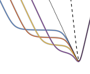
Figure 3 shows the marginal stability curves computed numerically from the unapproximated iNSE with the mechanical boundary conditions and from the iNSE with parameterised pumping boundary conditions for east–west rolls across a range of colatitudes. Respectively, these two model results are depicted by the underlying translucent grey curves and solid coloured curves. The representative case  $\varepsilon = 10^{-3}$
 $(Ek=10^{-9})$ is considered. Figure 3(a,b) illustrate the case for no-slip boundaries and figure 3(c,d) illustrate the stress-free case. Also included for reference are the asymptotic marginal stability curves obtained from the QG-RBC system (dotted curves).
Comparison of marginal stability curves and critical Rayleigh numbers vs wavenumber for the iNSE problem with physical (underlying translucent grey curves) and parameterised pumping boundary conditions (solid coloured curves) and the analytic results from the QG-RBC problem (dotted curves) also illustrated in figure 2. The case illustrated is  $\varepsilon = 10^{-3}$
 $(E=10^{-9})$ and
 $\chi = {\rm \pi}/2$ (east–west rolls) at various colatitudes
 $\vartheta _f$ (annotated). (a,b) No-slip boundaries. Excellent quantitative agreement exist between the iNSE and the CQG-RBC models. The significant impact of Ekman pumping on the onset of convection at low wavenumbers with respect to the QG-RBC model are the result of
 $O(E^{1/2})$ boundary layers is evident. (c,d) Results for stress-free boundaries illustrating excellent quantitative agreement between all models.

For stress-free boundaries, we observe excellent quantitative agreement for all wavenumbers between both iNSE models and the asymptotic results (dotted curves) from the QG-RBC system. This is consistent with the boundary-layer analysis of § 3 showing that the  $O(\varepsilon )$ pumping velocities emanating from Ekman layers adjacent to stress-free boundaries are too weak to induce corrections that alter the asymptotic predictions of the QG-RBC model. In effect, Ekman boundary layers, while necessary for the maintenance of stress-free boundaries, remain passive.
For no-slip boundaries results indicate excellent quantitative agreement between the two iNSE models for all wavenumbers illustrating the accuracy and fidelity of the parameterised pumping condition. However, figure 3 also reveals significant departures of the no-slip iNSE models from the stress-free QG-RBC results for low wavenumbers. Specifically, it is observed in the presence of no-slip boundaries,  $O(\varepsilon ^{1/2})$ pumping velocities from the Ekman layer act to further destabilise low-wavenumber (large-scale) modes and thereby extends the wavenumber range for steady convective onset at a fixed
 $\widetilde {Ra}$. This implies that at Rayleigh numbers above
 $\widetilde {Ra}_t$, when Ekman pumping is present, a wider range of wavenumbers are driving convection. The impact of Ekman pumping on the marginal curves is more clearly illuminated in the log–log plot (figure 3b) where departures from the stress-free marginal curves first occur through an intermediate region where the
 $\widetilde {Ra}$ remains approximately constant followed by a monotonic increase in
 $\widetilde {Ra}$ with decreasing
 $k_\perp$ that appears to parallel the asymptotic curve that scales with
 $\widetilde {Ra}\sim k_\perp ^{-2}$. Note, as predicted by (4.12a,b), the departure
 $(\widetilde {Ra}_t, k_{\perp t})$ from the stress-free marginal curves are increasing and decreasing functions of
 $\vartheta _f$, respectively.
Figure 4 illustrates that identical deductions hold for the CQG-RBC model with parameterised pumping boundary conditions. Indeed, this asymptotic model is in excellent quantitative agreement with both the iNSE models illustrated in figure 3. For stress-free boundary conditions, this result establishes the predicted equivalence between the CQG-RBC and QG-RBC models.
Marginal stability curves for the CQG-RBC problem with parameterised pumping boundary conditions (solid coloured curves) in comparison with the iNSE with physical boundary conditions (grey translucent curves) and the analytic results from the QG-RBC problem (dotted curves). Additional details are as in figure 3.

Figure 5 illustrates how the marginal stability boundaries for north–south rolls, the gravest mode, change as a function of  $\varepsilon$ for the CQG-RBC and the iNSE models with parameterised pumping boundary conditions (respectively, solid coloured curves and underlying translucent grey curves). Similar results hold for differing roll orientations. It is observed that the models are in excellent quantitative agreement, as
 $\varepsilon$ decreases the transition region is delayed but also extended in logarithmic range. Moreover, and quite remarkably, significant departures remain for geo- and astro-physically relevant values such as
 $\varepsilon =10^{-5}$ (i.e.
 $E=10^{-15}$) when compared with the asymptotic QG-RBC model (dotted line). The low-wavenumber departure from the QG-RBC model is consistent with the prediction detailed in (4.12a,b) indicating transitional wavenumber
 $|\boldsymbol {k}_{\perp t}|\sim \varepsilon ^{1/4}$ and Rayleigh number
 $\widetilde {Ra}_t\sim \varepsilon ^{-1/2}$ and always occurs within the rotationally constrained regime where
 $\widetilde {Ra}=o(\varepsilon ^{-1})$. Also consistent with (4.12a,b) is the delay in the transitional values as a function of roll orientation
 $\chi$, i.e. from north–south to east–west (as seen in figures 3 and 4).
Marginal stability curves with parameterised no-slip pumping conditions on CQG-RBC, for north–south convection rolls ( $\chi =0^\circ$) and varying rotational constraint
 $\varepsilon =\{10^{-2},10^{-3},10^{-4},10^{-5}\}$ (or, equivalently,
 $E=\{10^{-6},10^{-9},10^{-12},10^{-15}\}$). Underlying translucent grey curves and solid coloured curves represent the iNSE and CQG-RBC models, respectively. The black dashed line follows the maximal growth rate from the analytic quasi-geostrophic model, and the underlying blue dashed line is the maximal growth rate for iNSE with parameterised pumping at
 $\varepsilon = 10^{-5}$.

Figure 5 also illustrates that the loci of maximal growth rate with  $\widetilde {Ra}\propto k^{-1/8}_\perp$ remains insensitive to Ekman pumping (see dashed lines). Figure 6 expands on this point by illustrating a contour map for the growth rate in the
 $\widetilde {Ra}$–
 $k_\perp$ plane. One can observe that the marginal stability boundary for the asymptotic QG-RBC model strongly constrains the contours within it borders, however, the
 $O(1)$ effect of Ekman pumping distorts the exterior contours located at low wavenumbers. The inset illustrates a cross-section of the growth rate at fixed
 $\widetilde {Ra}=300$.
Contours of the growth rate for iNSE with no-slip pumping, at  $\vartheta _f = 0^\circ$,
 $\chi = 0^\circ$ and
 $\varepsilon = 10^{-3}$. The orange curve shows the marginal stability (where
 $s=0$), and the black dashed curve is the analytic quasi-geostrophic marginal curve given by (4.6). The blue dots mark the loci of the maximum growth rate for each value of
 $\widetilde {Ra}$. The light blue line shows a slice of the growth rate
 $s$ at
 $\widetilde {Ra} = 300$.

Figure 7 illustrates the asymptotic robustness of the parameterised boundary conditions by tracking the minimum critical values  $(\widetilde {Ra}_c,k_c)$ as a function of
 $\varepsilon$ (specifically the Taylor number
 $Ta=E^{-2}=\varepsilon ^{-6}$) for the sample colatitude
 $\vartheta = 75^\circ$. It can seen that parameterising the Ekman layer with pumping boundary conditions (3.16) quantitatively captures the departure from the asymptotic QG-RBC value (horizontal dashed line) for the onset of convection to relatively large
 $\varepsilon$ (i.e. small
 $Ta$) for all models. In the pertinent limit
 $\varepsilon \to 0$, the critical values approach the asymptotic result albeit slowly in the case of no-slip boundaries. For all boundaries, one may visually observe discernible differences between the iNSE with unapproximated boundary conditions and the iNSE with pumping boundary conditions around
 $Ta=10^{10}$ (i.e.
 $\varepsilon \sim 10^{-5/3}, \varepsilon \sim 10^{-5}$). We also observe that results from the asymptotic CQG-RBC model is in excellent quantitative agreement with those obtained from the iNSE. However, as
 $\varepsilon$ becomes large, departure from the iNSE model with exact boundary conditions occurs in an opposite manner to its iNSE counterpart with pumping boundary conditions. This may attributed to the absence of vertical momentum diffusion and the unbreakable constraint of geostrophy in the CQG-RBC model.
Critical reduced Rayleigh number and wavenumber vs Taylor number  $Ta$ (
 $=E^{-2} = \varepsilon ^{-6}$) for rolls (
 $\chi ={\rm \pi} /2$) at colatitudes
 $\vartheta _f = 0^\circ$ (a,b) and east–west rolls at
 $\vartheta _f = 5{\rm \pi} /12$ or
 $75^\circ$ (c,d). The blue curves correspond to no-slip boundary conditions and the red curves correspond to stress-free boundary conditions. Solid grey lines indicate solutions to the iNSE without approximation, and solid and dashed coloured lines correspond to solutions to the iNSE and CQG-RBC models, respectively, with pumping boundary conditions described in § 3.2. The asymptotic values for the QG-RBC given by (4.8a,b) and
 $k_c$ are shown by the horizontal dotted line in black.

A broader measure of the relative error between the critical onset of convection for the unapproximated iNSE problem and that with a parameterised pumping as function of roll orientation  $\chi$ and
 $\varepsilon$ is shown in figure 8 for colatitude
 $\vartheta _f = 75^\circ$. We observe that the error decays with
 $\varepsilon$ across all roll orientations
 $\chi$. For no-slip boundaries (figure 8a), we observe that the relative error is insensitive as a function of
 $\chi$ with an evolution to slightly greater accuracy occurring in the vicinity of north–south rolls
 $\chi < 15^\circ$. This is even more pronounced in the stress-free (figure 8b) case, but we observe a certain degree of non-monotonicity near the top of the plot at
 $\chi = 0$.
Relative error in critical Rayleigh number between the unapproximated iNSE and the iNSE with parameterised pumping, for  $\vartheta _f = 5{\rm \pi} /12$ (or
 $75^\circ$), plotted over a range of wavenumber angles
 $\chi$ and Taylor numbers
 $\varepsilon ^{-6}$: (a) no-slip boundary conditions and (b) stress-free conditions.

The eigenfunctions at the critical Rayleigh and wavenumber are shown for a mid-latitude,  $\vartheta _f = {\rm \pi}/4$,
 $\chi ={\rm \pi} /4$, and
 $\varepsilon = 10^{-3}$ in figure 9. This figure represents a direct illustration of the relaxation of spatial resolution constraints as a result of the utilisation of pumping boundary conditions. Only the outer (i.e. interior) solution,
 $\boldsymbol {v}^{(o)}$, is plotted on the full domain (first and third rows) since the full iNSE problem and interior iNSE problem with pumping boundary conditions are visually indistinguishable at this value of
 $\varepsilon$ except at the boundary. Within the Ekman boundary layer, figure 9(b,d) shows that the numerically computed full problem (open circles), the outer solution (dashed-dotted line) and the composite problem from the superposition of inner and outer solutions (solid line). The composite solutions appear to match quantitatively at leading order. Note that for no-slip case,
 $u^{(o)}$,
 $\zeta ^{(o)}$ and
 $w^{(o)}$ are all non-zero on the boundary, but the composite solution correctly captures the decay to zero. The same is true for
 $w^{(o)}$ in the stress-free case.
Profiles at the critical Rayleigh and wavenumbers for  $\vartheta _f = {\rm \pi}/4$,
 $\chi = {\rm \pi}/4$, and
 $\varepsilon = 10^{-3}$: (a,b) (blue curves) correspond to no-slip boundary conditions and (c,d) (red curves) correspond to stress-free boundary conditions. The solid lines show the interior solution on the full domain, and (b,d) show the Ekman boundary layer varying on the
 $O(\varepsilon ^{3/2})$ scale. The open circles are the numerically computed full problem, the solid line is the numerically computed interior solution with pumping boundary conditions, and the
 $\times$ are the composite solution (the numerically computed interior plus the analytic boundary layer).

In the lower row of figure 9, we plot the profiles for  $\boldsymbol {\hat {z}}\boldsymbol{\cdot}\boldsymbol {\nabla } (u,\zeta )$ in the stress-free case instead of just (
 $u$,
 $\zeta$), since this is the quantity used to set the pumping condition. In the immediate vicinity of the boundary, this shows slight differences between the solution with pumping and the exact stress-free boundary conditions that were not apparent if the derivative is not plotted. Figure 10 also illustrates this results as a hodograph of
 $\partial _{z} u$ vs
 $\partial _{z} v$ (the no-slip result
 $u$ vs
 $v$ is also included in the left plot). For the stress-free case, there is an observable
 $O(\varepsilon ^{1/2})$ error in
 $\partial _{z}(u,v)$ between the full and composite solutions due to the fact that the boundary condition (2.11b) is only satisfied to leading order in the composite solution. This may be understood as follows. Recall, a stress-free boundary requires
 \begin{equation} \boldsymbol{\hat{z}} \boldsymbol{\cdot}\boldsymbol{\nabla} \boldsymbol{v}\equiv (-\gamma \partial_{y} +\varepsilon\partial_{\varOmega}) \boldsymbol{v}^{(o)} + (-\gamma \partial_{y} + \delta \varepsilon^{-1/2} \partial_{\mu}) \boldsymbol{v}^{(i)} =0. \end{equation}
However, pumping boundary conditions are deduced from the leading-order expression
 \begin{equation} (-\gamma \partial_{y} +\varepsilon\partial_{\varOmega}) \boldsymbol{v}^{(o)} + \delta \varepsilon^{-1/2} \partial_{\mu} \boldsymbol{v}^{(i)} =0, \end{equation}
the difference being  $O(\gamma \partial _{y}\boldsymbol {v}^{(i)} ) = O(\varepsilon ^{1/2})$ given that
 $\boldsymbol {v}^{(i)}=O(\varepsilon ^{1/2})$.
Hodographs of the horizontal velocity in the Ekman layer for no-slip (a) and stress-free (b) problems for  $\varepsilon = 10^{-4}$,
 $\vartheta _f = {\rm \pi}/4$,
 $\chi = {\rm \pi}/4$ and critical
 $\widetilde {Ra}$ and wavenumber. For the no-slip case,
 $u$ is plotted against
 $v$, but for stress-free case we show
 $\partial _{z}u$ vs
 $\partial _{z}v$. The open circles denote the numerically computed full problem, and the
 $\times$ are the composite solution (the numerically computed interior plus the analytic boundary layer).

5. Strongly nonlinear solutions
5.1. The QG-RBC model
The QG-RBC equations (2.14) admit exact steady nonlinear single-mode solutions of the form
 \begin{equation} (w_0, \theta_1) =(\hat w,\hat \theta)(\varOmega) h(x,y) + \text{c.c.},\quad \psi_0 = {(\hat \psi(\varOmega) h(x,y) + \frac{\gamma}{k_\perp^2} \hat w(\varOmega) h_x(x,y)) + \text{c.c.}}, \end{equation}
with
 \begin{equation} \hat \theta(\varOmega) ={-\frac{ \sigma}{k_\nabla^2} (\partial_{\varOmega}\bar{\varTheta}_0 -1) \hat w(\varOmega)}. \end{equation}
Here  $h(x,y)$ satisfies the planform equation
 $\nabla ^2_\perp h = - {k}_{\nabla }^2 h$. Single-mode solutions require the Jacobian advection terms in the QG-RBC (2.14) be identically zero under this ansatz. We note, the only such solutions for
 $\gamma \ne 0$ are roll solutions
 $h(x,y)=\exp ( ik_x x+ik_y y)$. Single-mode solutions are known to be unstable to fully 3D multimodal perturbations (Sprague et al. Reference Sprague, Julien, Knobloch and Werne2006), however, they provide a skeletal framework for dynamical trajectories within phase-space and, thus, highly influence the evolution of realised solutions. Here again, the dependence of
 $\psi$ within the expression for vertical motions
 $\hat w(\varOmega )$ is a reflection of the non-axial buoyant driving of axial vorticity. The amplitudes
 $\hat w(\varOmega ), \hat \psi (\varOmega )$ and mean temperature gradient
 $\partial _{\varOmega } \bar {\varTheta }-1$ satisfy the coupled ODE system
 $$\begin{gather} \partial_{\varOmega} \hat w + k_\perp^2 k_\nabla^2 \hat \psi =0,\quad \partial_{\varOmega} \hat \psi - \left({\frac{\widetilde{Ra} Nu }{ k_\nabla^2 + 2\sigma^2 \vert\hat w\vert^2}} - \frac{k_\nabla^4}{k_\perp^2}\right) \hat w =0, \end{gather}$$
 $$\begin{gather}\partial_{\varOmega} \bar{\varTheta}_0 -1 = {-\frac{k_\nabla^2 Nu }{k_\nabla^2 + 2\sigma^2 \vert\hat w\vert^2}} , \end{gather}$$
with Nusselt number
 \begin{equation} Nu = \left[\int_0^1 \frac{k_\nabla^2}{k_\nabla^2 + 2\sigma^2 \vert\hat w\vert^2} {\rm d} \varOmega \right]^{-1} \end{equation}
measuring the non-dimensional heat transport. Without loss of generality, the dependency of  $\sigma$ can be absorbed by rescaling amplitudes according to
 $(w_0,\psi _0,\theta _1)\mapsto (w_0,\psi _0,\theta _1)/\sigma$. System (5.2) is accompanied with impenetrable boundary conditions
 $\hat w(0)=\hat w(1) =0$. Equations (5.2a,b) may also be collapsed to
 \begin{equation} \partial_{\varOmega\varOmega} \hat w + k^2_\perp k^2_\nabla \left(\frac{\widetilde{Ra} Nu}{k^2_\nabla + 2 \sigma^2 \vert \hat w\vert^2} - \frac{k_\nabla^4}{k_\perp^2}\right) \hat w = 0,\quad w(0)=\hat w(1) =0. \end{equation}
The single-mode analysis of Grooms (Reference Grooms2015) for the upright QG-RBC may be extended to the tilted  $f$-plane for both the QG-RBC with impenetrable boundaries and CQG-RBC with stress-free pumping conditions. Ensuring that all terms in (5.3a,b) are dominant at the midplane
 $\varOmega =0.5$ requires
 \begin{equation} \vert \hat w(0.5) \vert^2 \sim \frac{k^2_\perp}{k^4_\nabla} \widetilde{Ra} Nu, \quad\implies\quad \partial_{\varOmega}\bar{\varTheta}(0.5) - 1\sim \frac{k^6_\nabla}{k^2_\perp}\frac{1}{\widetilde{Ra}},\quad \epsilon > 0. \end{equation}
The latter result follows from (5.2c). Along loci  $k_\perp \propto \widetilde {Ra}^\alpha$, Grooms (Reference Grooms2015, (33) and (41)) has established the sharp bounds
 \begin{equation} \widetilde{Ra}^{1+2\alpha} \le Nu \le \widetilde{Ra}^{1+2\alpha}\ln (\widetilde{Ra}^{1-4\alpha} Nu) \sim \widetilde{Ra}^{1+2\alpha + \epsilon} \end{equation}
for  $-1/2\le \alpha \le 1/4$ in QG-RBC, which imply
 \begin{equation} \partial_{\varOmega}\bar{\varTheta}(0.5) - 1\sim \widetilde{Ra}^{4\alpha -1}. \end{equation}
We note that the analysis for the CQG-RBC with no-slip pumping boundary conditions remains an open problem. Thus, as points of reference for comparison the QG-RBC (or CQG-RBC with stress-free boundary conditions) give
 \begin{equation} \left.\begin{gathered} k_\perp= \mathrm{fixed},\quad \alpha=0,\quad \implies\quad \partial_{\varOmega}\bar{\varTheta}\sim \widetilde{Ra}^{-1},\\ k_\perp= \widetilde{Ra}^{1/4},\quad \implies\quad \partial_{\varOmega}\bar{\varTheta}\sim \mathrm{const.} \end{gathered}\right\} \end{equation}
The scaling exponent  $\alpha =1/4$ corresponds to the maximal heat transport for the single-mode solutions in QG-RBC and provides the upper bound
 $Nu\sim \widetilde {Ra}^{3/2}$ compared with the fixed wavenumber case where
 $Nu\sim \widetilde {Ra}$.
5.2. The CQG-RBC model
Single-mode solutions to the CQG-RBC model of the form (5.1) may be pursued upon neglecting nonlinear vertical advection of temperature fluctuation in (3.22c) that are significant in the thermal wind layer. This results in the complex-valued system
 $$\begin{gather} \partial_{\varOmega} \hat w + k_\perp^4 (1+ \gamma^2 \sin^2 \chi) \hat \psi = 0, \end{gather}$$
 $$\begin{gather}\partial_{\varOmega} \hat \psi + k_\perp^2 (1+ \gamma^2 \sin^2 \chi)^2 \hat w = {\frac{\widetilde{Ra}}{\sigma}} \hat\theta, \end{gather}$$
 $$\begin{gather}\sigma (\partial_{\varOmega} \bar{\varTheta}_0 - 1) \hat w = [\varepsilon^2 \partial_{\varOmega\varOmega} - k_\perp^2 (1+ \gamma^2 \sin^2 \chi) - 2 {\rm i} \varepsilon \gamma k_\perp \sin\chi \partial_{\varOmega}] \hat \theta, \end{gather}$$
 $$\begin{gather}\sigma \partial_{\varOmega} (\hat w \hat \theta^* + \text{c.c.}) = \partial_{\varOmega\varOmega} \bar{\varTheta}_0. \end{gather}$$
System (5.8) is accompanied with fixed-temperature conditions  $\hat \theta (0)=\hat \theta (1)=0$, and no-slip pumping boundary conditions given in (3.16). Recall that for stress-free pumping boundary conditions the CQG-RBC is equivalent to the QG-RBC.
5.3. Results: fully nonlinear single-mode solutions
Investigations of single-mode solutions to the QG-RBC model (5.2) have been performed by Grooms (Reference Grooms2015) and Julien & Knobloch (Reference Julien and Knobloch1998) in the absence of Ekman pumping for the upright and tilted  $f$-plane cases, respectively. Julien et al. (Reference Julien, Aurnou, Calkins, Knobloch, Marti, Stellmach and Vasil2016) explored the impact of pumping boundary conditions for upright RRBC. Such solutions are asymptotically accurate but unstable solutions to the RRBC problem in the rapidly rotating limit
 $\varepsilon \rightarrow 0$. In totality, at a fixed
 $\widetilde {Ra}$ these solutions may be interpreted as the skeletal structure of the high-dimensional phase space that all realised solution trajectories must navigate. Hence, under the assumption that they possess a close proximity to the realised fluid state, the global properties of single-mode solutions are informative. Here, fully nonlinear single-mode roll solutions are investigated in the
 $\widetilde {Ra}$ vs
 $k_\perp$ plane via a simulation suite of the CQG-RBC model (5.8) with no-slip pumping boundary conditions at arbitrary
 $\vartheta _f$. This is compared with an identical simulation suite for the QG-RBC model that has been established as equivalent to the CQG-RBC model with stress-free pumping conditions.
In figure 11, contour plots are illustrated at  $\varepsilon =10^{-2}$ for
 $Nu$,
 $Re = \max (\vert \hat w\vert )$, and midplane mean temperature gradient
 $\partial _{\varOmega }\bar {T} = \partial _{\varOmega }\bar {\varTheta }_0-1$ obtained from the CQG-RBC model on the tilted
 $f$-plane for north–south rolls at any arbitrary
 $\vartheta _f< 90^\circ$, (figure 11a–c). We recall, based on the colatitudinal Rayleigh number
 $\widetilde {Ra}$, north–south rolls have the same linear and nonlinear stability properties at any given
 $\vartheta _f$. As a function of
 $\widetilde {Ra}$ at fixed
 $k_\perp$ it can be observed from the contours that
 $Nu$ and
 $Re$ are monotonically increasing functions of
 $\widetilde {Ra}$ while
 $\partial _{\varOmega }\bar {T}$ is a monotonically decreasing function of
 $\widetilde {Ra}$ indicating approach to an isothermal interior. In figure 12, the opposite bookend case for east–west rolls is illustrated at colatitudinal location
 $\vartheta _f= 75^\circ$ and display identical features to the north–south case in figure 11 albeit for delayed
 $\widetilde {Ra}$ due to the increased stability of this roll orientation (see figure 12(a–c)). Note that
 $\widetilde {Ra}/\widetilde {Ra}_c < \varepsilon ^{-1}$, so we are still within the domain of validity.
The CQG-RBC model with no-slip pumping boundary conditions evaluated on tilted  $f$-plane for north–south rolls at any arbitrary
 $\vartheta _f< 90^\circ$ with
 $\varepsilon = 10^{-2}$. (a–c) Contours of
 $Nu$,
 $Re$ and
 $\partial _\varOmega \bar {T}$ at the midplane in the
 $k_\perp$ vs
 $\widetilde {Ra}$ plane. The solid blue denotes the marginal stability curve. For comparison, the dotted black line is the analytic quasi-geostrophic marginal stability curve where pumping is omitted. (d–f) Plots of
 $Nu$,
 $Re$ and
 $\partial _\varOmega \bar {T}$ as a function of
 $\widetilde {Ra}$ along loci for maximal values at each
 $\widetilde {Ra}$ (red solid line), maximal linear growth rate
 $s$ (yellow curve) and fixed critical wavenumber
 $k_{\perp c}$ (blue dotted line). For comparison, results for the quasi-geostrophic model along identical loci are illustrated (grey lines).

The CQG-RBC model with no-slip pumping boundary conditions evaluated on the tilted  $f$-plane at
 $\vartheta _f=75^\circ$ for east–west rolls (
 $\chi = 90^\circ$) with
 $\varepsilon = 10^{-2}$. Labelling is as in figure 11.

The  $Nu$,
 $Re$ and
 $\partial _{\varOmega }\bar {T}$ values that appear in figures 11(a–c) and 12(a–c) are plotted as a function of
 $\widetilde {Ra}$ along different loci in figures 11(d–f) and 12(d–f), respectively (coloured lines). These values are taken along the two loci highlighted in figures 11(a–c) and 12(a–c): maximal linear growth rate (which is proportional to
 $k^{-8}_\perp$) and extremal values
 $k_{max}$ achieved at a fixed
 $Ra $, as well as along fixed value
 $k_{c\perp }$. These loci are motivated by linear marginal onset, recent simulations of the QG-RBC that find that integral length scale of convection follows the maximal growth rate (Oliver et al. Reference Oliver, Jacobi, Julien and Calkins2023), and exploration of optimal global transport of heat and momentum. For comparison, results along the equivalent loci are given for the QG-RBC model that omits pumping (grey lines). As established, this is equivalent to the CQG-RBC with stress-free pumping conditions. It is evident that Ekman pumping in presence of no-slip boundaries significantly enhances the global heat and momentum transport as measured by Nusselt number
 $Nu$ and Reynolds number
 $Re$. It is observed that the lineplots for
 $Nu$ in the CQG-RBC model are insensitive to the particular choice of locus. Thus, we consider fixed
 $k_\perp$ and
 $k_{max}$ as the representative markers, and plot for guidance scaling lines
 $Nu\sim \widetilde {Ra}^1$ and
 $Nu\sim \widetilde {Ra}^{3/2}$,
 $Re = \vert \hat w(0.5)\vert \sim \widetilde {Ra}^1$ and
 $\partial _{\varOmega }\bar {\varTheta }\sim Ra^{-1}$ established for the QG-RBC model (see (5.7)), and by experiment in Bouillaut et al. (Reference Bouillaut, Miquel, Julien, Aumaître and Gallet2021). It can be seen that curves associated with loci of
 $k_\perp$ fixed and extrema for
 $Nu$,
 $Re$ and
 $\partial _{\varOmega }\bar {T}$ are in compliance with these estimates. Thus, the impact of Ekman pumping appears to reside in the prefactor, consistent with the findings of Plumley et al. (Reference Plumley, Julien, Marti and Stellmach2017). However, instantaneous scaling exponents along curves of maximal growth rate
 $k_\perp \propto \widetilde {Ra}^{-1/8}$ appear consistently smaller for
 $Re$ and
 $\partial _{\varOmega }\bar {T}$. This is an expected result given that the single-mode theory is one that captures nonlinear stationary states and, thus, excludes consideration of maximal growth solutions. Consequently, loci tracking maximal values of contours at fixed
 $\widetilde {Ra}$ constitute upper bounds.
These qualitative features illustrated in figures 11 and 12 extend to cases with decreasing  $\varepsilon$ across all colatitudes
 $\vartheta _f < 90^\circ$ (see also Julien et al. Reference Julien, Aurnou, Calkins, Knobloch, Marti, Stellmach and Vasil2016). As with the linear results,
 $Nu$ and
 $Re$ vs
 $\widetilde {Ra}$ for the CQG-RBC model experiences a delayed departure from that observed in the QG-RBC model as
 $\varepsilon$ decreases. However, the transition to a power law scaling is increasingly abrupt as
 $\varepsilon$ decreases and the larger values of
 $Nu$ and
 $Re$ are observed as in Julien et al. (Reference Julien, Aurnou, Calkins, Knobloch, Marti, Stellmach and Vasil2016).
6. Discussion and conclusion
The boundary-layer reduction of RRBC in the limit of rapid rotation is considered on the tilted  $f$-plane located at arbitrary colatitude
 $\vartheta _f< 90^\circ$. As a consequence of gyroscopic alignment occurring through the Taylor–Proudman constraint, spatial variations of fluid structures along the axis of rotation are observed to be
 $O(H)$ as compared with
 $O(E^{1/3}H)$ along
 $\boldsymbol {\hat {z}}$ (i.e. radial) direction. This motivates the use of a non-orthogonal coordinate system representation where the upright coordinate aligns with the rotation axis as opposed to gravity. A matched asymptotic analysis is performed on the iNSEs that govern the fluid dynamics. Three regions are identified and matched asymptotically: a geostrophic interior whose velocity and thermal fields are rectified by an inner Ekman boundary layer of
 $O(E^{1/2} H)$ and a middle thermal wind layer of
 $O(E^{1/3} H)$, respectively. The analysis reveals that these boundary layers obey classical equation sets but evolve with the boundary-layer coordinates that align with the rotation axis. Specifically, an analysis of the Ekman layer yields the fourth-order ODE system resulting from the Coriolis–viscous force balance (Greenspan Reference Greenspan1969). Mass continuity then uncovers parameterised boundary conditions which serves as the kinematic condition that circumvents the numerical spatial resolution requirements of a viscous layer and captures the effects of Ekman pumping and suction. Closure of the iNSE system that utilises this kinematic condition requires it be supplemented with geostrophic boundary conditions serving as the mechanical boundary conditions for the interior dynamics. By contrast, for the non-hydrostatic quasi-geostrophic equations (i.e. QG-RBC and CQG-RBC) constituting the asymptotic reductions of the iNSE in the limit of rapid rotation, no mechanical boundary conditions are required. The thermal wind layers are in geostrophic and axial hydrostatic balance, the latter balance ensuring thermal fluctuations that maintain fixed temperature boundary conditions.
In the presence of no-slip boundaries, the parameterised boundary condition is the vertical velocity/vertical vorticity pumping relationship,  $w\propto \varepsilon ^{1/2} \zeta$, or in dimensional terms,
 $w^*\propto (\nu /2\Omega \cos \vartheta _f)^{1/2} \zeta ^*$. This is known in the literature through its application to large-scale atmospheric and oceanic flows (Vallis Reference Vallis2006) but less familiar to convectively driven flows. Linear stability investigations of the iNSE and the CQG-RBC with parameterised pumping boundary conditions reveal that they are a quantitatively accurate alternate to the unapproximated problem where Ekman boundary layers are unfiltered. Importantly, to the best of the authors’ knowledge, it is demonstrated for the first time that Ekman pumping strongly destabilises large-scale (low-wavenumber) convective modes and, thus, significantly extended the spatial range of convectively unstable modes at fixed
 $\widetilde {Ra}$. It is established that this occurs when pumping velocity
 $w\sim O(1)$ which is always achieved in the quasi-geostrophic regime established to have the upper bound
 $\zeta =o(\varepsilon ^{-1})$. This implies some caution should be taken not to truncate the dynamical regime in selecting the aspect ratio of computational domains in plane-layer investigations of RRBC.
For stress-free boundary conditions, the asymptotic analysis uncovered the vertical velocity/vertical gradient of vertical vorticity pumping relationship,  $w\propto \varepsilon \hat{\boldsymbol {{z}}} \boldsymbol{\cdot}\boldsymbol {\nabla } \zeta$, or, in non-dimensional terms,
 $w^*\propto (\nu /2\Omega \cos \vartheta _f) \hat{\boldsymbol{z}} \boldsymbol{\cdot}\boldsymbol {\nabla }^* \zeta ^*$. Linear stability theory of the iNSE and CQG-RBC with pumping boundary conditions again reveal excellent quantitative agreement with the iNSE without approximation. In fact, it is found that all three of these models are accurately captured by the QG-RBC constrained only by the requirement of impenetrable boundary conditions. This is supported by the observation that the pumping velocity always remains subdominant in the quasi-geostrophic regime where
 $\zeta =o(\varepsilon ^{-1})$. Thus, Ekman boundary layers while present remain passive. The pumping boundary conditions for this case thus serve solely as a means of filtering these layers thus providing relief on the numerical spatial resolution requirements.
Results from DNS with imposed pumping conditions will be pursued in the future, as this has the potential to reduce computational cost by removing the need to resolve the  $O(Ek^{1/2}H)$ Ekman boundary layer. As an intermediate step, results for single-mode solutions to the CQG-RBC model were presented for both no-slip and stress-free boundary conditions. It is demonstrated that pumping in the presence of no-slip boundaries greatly enhance the global heat and momentum transport properties of the fluid layer to the remarkable extent that an
 $O(E^{1/2} H)$ layer generates
 $\Delta Nu, \Delta Re = O(1)$. We also see that the heat transport remains of similar magnitude across tilt angles, though it occurs on a shifted domain of
 $\widetilde {Ra}$ numbers. We note that the single-mode solutions, while instructive, omit an important phenomenon, i.e. the lateral stirring and mixing of thermal field. As such, the mean temperature field does not saturate to an unstable profile as
 $\widetilde {Ra}\rightarrow \infty$ as observed in fully nonlinear simulations (Julien et al. Reference Julien, Legg, McWilliams and Werne1996; Sprague et al. Reference Sprague, Julien, Knobloch and Werne2006; Julien et al. Reference Julien, Rubio, Grooms and Knobloch2012). Instead, it continues to an isothermal interior;
 $\partial _{\varOmega } \overline {T}\sim \widetilde {Ra}^{-1}$ for stress-free boundaries. This feature is inherent to the single-mode approximation including recent works of Barker, Dempsey & Lithwick (Reference Barker, Dempsey and Lithwick2014) and Currie et al. (Reference Currie, Barker, Lithwick and Browning2020) based on the original work of Stevenson (Reference Stevenson1979) that report mean temperature gradient power laws that evolve to isothermality.
Acknowledgements
K.J. thanks Dr G. Vasil for fruitful interactions and discussions and Dr J. Aurnou for useful remarks on the manuscript.
Funding
This work was supported by the National Science Foundation (grant no. DMS-2308337).
Declaration of interests
The authors report no conflict of interest.
Appendix A. Mixed vorticity–velocity formulation
The primitive variable formulation of the linearised iNSE (2.8) in the main text is of ninth order in  $\varOmega$. Specifically, the continuity equation requires the imposition of a ninth auxiliary boundary condition applied to the pressure function
 $p$. Instead of pursuing this option, we numerically solve the following modified set of equations for the variables
 $\boldsymbol {u}= u \boldsymbol {\hat {x}} + (v-\gamma w) \boldsymbol {\hat {y}} + w/\eta _3 \boldsymbol {\hat {\eta }}$,
 $\boldsymbol {U}_\perp =U^g\boldsymbol {\hat {x}} + V^g\boldsymbol {\hat {y}}$,
 $\boldsymbol {\omega }=\omega ^1 \boldsymbol {\hat {x}} + \omega ^2 \boldsymbol {\hat {y}} + \zeta /\eta _3 \boldsymbol {\hat {\eta }}$,
 $p$ and
 $\theta '$:
 $$\begin{gather} \omega^1 = \partial_{y}(w+\gamma v) -\varepsilon \partial_{\varOmega} v, \end{gather}$$
 $$\begin{gather}\omega^2 =-\partial_{x}(w+\gamma v) +\varepsilon \partial_{\varOmega}u, \end{gather}$$
 $$\begin{gather}\zeta = \partial_{x}v-\partial_{y}u, \end{gather}$$
 $$\begin{gather}U^g = \varepsilon^{-1}(u+\partial_{y}p), \end{gather}$$
 $$\begin{gather}V^g = \varepsilon^{-1} (v-\gamma w) - \partial_{x}p, \end{gather}$$
 $$\begin{gather}\partial_{t} u - V^g = (\varepsilon \partial_{\varOmega}- \gamma\partial_{y})\omega^2+ \left(\varepsilon \gamma\partial_{\varOmega}-\frac{1}{\eta_3^2}\partial_{y} \right) \zeta, \end{gather}$$
 $$\begin{gather}\partial_{t} (v -\gamma w) + \frac{1}{\eta_3^2}U^g =-\varepsilon\partial_{\varOmega}\omega^1 + \gamma \partial_{x} \omega^2+\frac{1}{\eta_3^2}\partial_{x}\zeta +\gamma \partial_{\varOmega}p - \frac{\gamma \widetilde{Ra}}{ \sigma} \theta ,\end{gather}$$
 $$\begin{gather}\partial_{t} w +\gamma U^g = \frac{1}{\eta_3} ({\gamma}\partial_{x}\zeta -\partial_{y}\omega^1 + \partial_{x}\omega^2) + \partial_{\varOmega}p + \frac{\widetilde{Ra} }{\sigma} \theta , \end{gather}$$
 $$\begin{gather}\partial_{t} \theta - w = \frac{1}{\sigma} \left(\partial_{x}^2\theta+\frac{1}{\eta_3^2}\partial_{y}^2\theta - 2\varepsilon\gamma \partial_{y}\partial_{\varOmega} \theta +\varepsilon^2 \partial_{\varOmega}^2 \theta\right), \end{gather}$$
 $$\begin{gather}\partial_{x} U^g +\partial_{y} V^g +\partial_{\varOmega}w = 0. \end{gather}$$
This is a closed formulation that remains eighth order, i.e. compatible with either the number of physical or pumping boundary conditions presented in table 1.
A.1. Boundary conditions
In the mixed vorticity–velocity formulation, we may avoid setting boundary conditions on the mixed derivative  $\boldsymbol {\hat {z}} \boldsymbol{\cdot}\boldsymbol {\nabla }$ by using the following identities. For the unapproximated stress-free iNSE problem,
 $$\begin{gather} \boldsymbol{\hat{z}} \boldsymbol{\cdot}\boldsymbol{\nabla} u = \omega^2 +\gamma \zeta \quad \mbox{on}\ \varOmega = 0,1, \end{gather}$$
 $$\begin{gather}\boldsymbol{\hat{z}} \boldsymbol{\cdot}\boldsymbol{\nabla} v = \omega^1\quad \mbox{on}\ \varOmega = 0,1, \end{gather}$$
so the mixed boundary conditions on  $u$ and
 $v$ become Dirichlet conditions on
 $\omega ^1$ and
 $\omega ^2+\gamma \zeta$. For the parameterised iNSE stress-free problem,
 \begin{equation} \boldsymbol{\hat{z}} \boldsymbol{\cdot}\boldsymbol{\nabla} \zeta =-(\partial_{x} \omega^1 + \partial_{y}(\omega^2 +\gamma \zeta)), \end{equation}
so the pumping boundary condition (3.16b) can be formulated as a Dirichlet condition on  $\omega ^1$,
 $\omega ^2$ and
 $\zeta$.
Appendix B. Numerics
B.1. Linear problems
For the linear stability problem, we assume solutions of the form
 \begin{equation} \begin{pmatrix} \omega^1 \\ \omega^2 \\ \zeta \\ u \\ v\\ w \\ p\\ \theta \end{pmatrix} = \begin{pmatrix} \hat{\omega}^1 \\ \hat{\omega}^2 \\ \hat{\zeta} \\ \hat{u} \\ \hat{v}\\ \hat{w}\\ \hat{p}\\ \hat{\theta} \end{pmatrix}\exp (st + {\rm i}k_x x +{\rm i}k_y y). \end{equation}
We expand the fluid variables in a recombined Chebyshev basis which makes applying boundary conditions sparse. For almost all variables, we use the expansion
 \begin{equation} \sum_{n=0}^{N-1}c_{(n)}\varphi_n(r), \end{equation}
where  $r = 2\varOmega -1 \in [-1,1]$, and
 $\varphi _n$ is a Dirichlet bases (Burns et al. Reference Burns, Vasil, Oishi, Lecoanet and Brown2020), i.e. a Chebyshev Galerkin polynomials given by
 \begin{align} \varphi_0(r) = T_0(r) = 1,\quad \varphi_1(r) = T_1(r) = r,\quad \varphi_n(r) = T_n(r)-T_{n-2}(r) \quad \mbox{for}\ n\geq 2, \end{align}
where  $T_n(r) = \cos (n\arccos (r))$ are the standard Chebyshev polynomials. Then
 $\varphi _n(\pm 1) = 0$ for
 $n\geq 2$, so all that is required to enforce a Dirichlet boundary condition at the top and bottom are the equations
 \begin{equation} c_{(0)} \pm c_{(1)} = 0, \end{equation}
independent of  $N$. For the stress-free pumping boundary conditions we require a mixed derivative
 $\boldsymbol {\hat {z}} \boldsymbol{\cdot}\boldsymbol {\nabla }$, so we use the basis
 $$\begin{gather} \psi_m = T_m,\quad m = 0,1,2,3, \end{gather}$$
 $$\begin{gather}\psi_m = T_{m-4} - \frac{2(m-2)}{m-1} T_{m-2}+\frac{m-3}{m-1} T_m, \quad m = 4,5,\ldots,N-1, \end{gather}$$
(Julien & Watson Reference Julien and Watson2009). In this basis,  $\psi _m(\pm 1) = \psi _m'(\pm 1) = 0$ for
 $m\geq 4$, so
 \begin{align} & (\boldsymbol{\hat{z}} \boldsymbol{\cdot}\boldsymbol{\nabla}) \left.\sum_{m=0}^{N-1} c_{(m)}\psi_m\right\rvert_{r ={\pm} 1} = \left.\sum_{m=0}^{N-1} c_{(m)}(2\varepsilon \partial_{r}-{\rm i}k_y \gamma) \psi_m \right\rvert_{r ={\pm} 1} \nonumber\\ &=2 \varepsilon (c_{(0)}\pm c_{(1)}+ c_{(2)}\pm c_{(3)}) -{\rm i}k_y \gamma (c_{(1)}\pm 4 c_{(2)} +9 c_{(3)}), \end{align}
so enforcing this boundary condition is also independent of  $N$. We also employ a quasi-inverse technique to treat the vertical derivatives.
B.2. Nonlinear problems
We solve the nonlinear single-mode problem using MATLAB's bvp5c. This requires a first-order formulation. In order to ensure real-valued variables, we write the roll ansatz as sines and cosines,
 $$\begin{gather} w_0 = w_c \cos(k_x x+k_y y) + w_s \sin(k_x x +k_y y), \end{gather}$$
 $$\begin{gather}\theta_1 = \theta_c \cos(k_x x+k_y y) + \theta_s \sin(k_x x +k_y y), \end{gather}$$
 $$\begin{gather}\psi_0 = \psi_c \cos(k_x x+k_y y) + \psi_s \sin(k_x x +k_y y )+\frac{\gamma}{k_x^2+k_y^2} \partial_{x} w_0, \end{gather}$$
substituted into the CQG-RBC (3.22) yields the real-valued system
 $$\begin{gather} \partial_{\varOmega}w_s =-k_p^2(k_x^2+k_y^2)\psi_s, \end{gather}$$
 $$\begin{gather}\partial_{\varOmega}w_c =-k_p^2(k_x^2+k_y^2)\psi_c, \end{gather}$$
 $$\begin{gather}\partial_{\varOmega}\psi_s = \frac{\widetilde{Ra}}{\sigma} \theta_s - \frac{k_p^4}{k_x^2+k_y^2} w_s, \end{gather}$$
 $$\begin{gather}\partial_{\varOmega}\psi_c = \frac{\widetilde{Ra}}{\sigma} \theta_c - \frac{k_p^4}{k_x^2+k_y^2} w_c, \end{gather}$$
 $$\begin{gather}\frac{\varepsilon^2}{\sigma} \partial_{\varOmega}^2 \theta_s = \sigma w_s (w_c\theta_c + w_s \theta_s) - Nu w_s + \frac{k_p^2}{\sigma} \theta_s - \frac{2 \varepsilon \gamma k_y}{\sigma} \partial_{\varOmega}\theta_c, \end{gather}$$
 $$\begin{gather}\frac{\varepsilon^2}{\sigma} \partial_{\varOmega}^2 \theta_c = \sigma w_c (w_c\theta_c + w_s \theta_s) - Nu w_c +\frac{k_p^2}{\sigma} \theta_c + \frac{2 \varepsilon \gamma k_y}{\sigma} \partial_{\varOmega}\theta_s. \end{gather}$$


 Open access

