



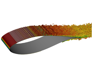





1. Introduction
System rotation may engender various types of flow instabilities, as demonstrated for channel flows subject to spanwise rotation (Hart Reference Hart1971; Lezius & Johnston Reference Lezius and Johnston1976), in which regularly spaced stationary streamwise vortices appear at a lower Reynolds number than Tollmien–Schlichting (TS) waves (Tritton & Davies Reference Tritton and Davies1985; Alfredsson & Persson Reference Alfredsson and Persson1989). Transition to turbulence occurs through the secondary instability of these vortices, characterised by their twisting (Alfredsson & Persson Reference Alfredsson and Persson1989; Wall & Nagata Reference Wall and Nagata2006). Experiments indicate that cyclonic rotation (parallel to mean vorticity/shear) is stabilising, whereas anticyclonic rotation (antiparallel to mean vorticity/shear) is destabilising (Koyama et al. Reference Koyama, Masuda, Ariga and Watanabe1979). This effect also occurs in Blasius (Potter & Chawla Reference Potter and Chawla1971; Dechamps & Hein Reference Dechamps and Hein2018) and turbulent (Tritton Reference Tritton1992) boundary layers. The stabilisation engendered by cyclonic rotation reduces the receptivity to free stream disturbances (Masuda & Matsubara Reference Masuda and Matsubara1990) and changes the optimal perturbation from streamwise vortices (low rotation) to spanwise vortices (high rotation) (Yecko & Rossi Reference Yecko and Rossi2004).
More relevant to wind turbine applications are the configurations in which the rotation axis is orthogonal to the spanwise direction. The generated cross-flow profiles may be prone to inflectional (cross-flow) instability (Saric, Reed & White Reference Saric, Reed and White2003). The rotating disk (von Kármán Reference von Kármán1921) epitomises such flow configuration, where cross-flow vortices form an angle of  $14^\circ$ to the radius (Gregory, Stuart & Walker Reference Gregory, Stuart and Walker1955). Stability analyses by Malik (Reference Malik1986) allowed obtaining the neutral curve for stationary disturbances. Balachandar, Streett & Malik (Reference Balachandar, Streett and Malik1992) showed a primary disturbance root mean square (r.m.s.) amplitude of
 $9\,\%$ of the disk rotation speed for the inception of secondary instability, characterised by counter-rotating vortices superimposed on the cross-flow structures. Short-wavelength vortices are more susceptible to secondary instability but not the most amplified primary disturbances. The presence of axial flow reduces the amplification of the cross-flow instability as the cross-flow profiles become less inflectional (Garrett, Hussain & Stephen Reference Garrett, Hussain and Stephen2010), which may explain the irrelevance of cross-flow modes to transition in the wind turbine blade study of Jing, Ducoin & Braud (Reference Jing, Ducoin and Braud2020). The rotating disk flow is convectively stable in the circumferential direction but absolutely unstable in the radial direction above a critical radius-based Reynolds number (Lingwood Reference Lingwood1995, Reference Lingwood1996), explaining the insensitivity of transition to the disturbance level (Malik, Wilkinson & Orszag Reference Malik, Wilkinson and Orszag1981). The marine propeller investigated by Jing & Ducoin (Reference Jing and Ducoin2020) displayed similar instability mechanisms to the rotating disk.
Regarding fan blades, cross-flow modes driven by rotation seem too weak to trigger transition (Pascal et al. Reference Pascal, Barrier, Billonet and Marty2020; Theiss et al. Reference Theiss, Hein, Pascal and Cliquet2022), even though their growth rates tend to increase with the rotation rate (Dechamps & Hein Reference Dechamps and Hein2018). Likewise, experiments showed that transition on a rotating helicopter blade occurred via two-dimensional TS waves, with rotation not affecting the transition location (Weiss et al. Reference Weiss, Gardner, Klein and Raffel2017, Reference Weiss, Gardner, Schwermer, Klein and Raffel2019, Reference Weiss, Wolf, Kaufmann, Braukmann, Heineck and Raffel2020). This may be due to the attached character of the flow, where Coriolis and centrifugal forces are in balance, and there is a low cross-flow (McCroskey Reference McCroskey1971). Other experiments on rotating aeronautical propellers showed that the flow transitioned to turbulence over a laminar separation bubble (LSB), whose starting point shifted abruptly to the leading edge above a critical radius (Schülein, Rosemann & Schaber Reference Schülein, Rosemann and Schaber2012; Lang et al. Reference Lang, Gardner, Mariappan, Klein and Raffel2015). The role of rotation and spanwise flow in this mechanism is unclear. Toppings & Yarusevych (Reference Toppings and Yarusevych2023) observed an increased spanwise velocity inside LSBs near a stationary wing tip and root, triggering modes travelling in the same direction as this flow. In the case of a swept LSB, the literature suggests that a self-excited LSB instability is little affected by the cross-flow (Hosseinverdi & Fasel Reference Hosseinverdi and Fasel2016).
In the few detailed numerical simulations regarding the stability of rotating wind turbine blades, rotation-induced cross-flow instability was observed in some cases (Gross et al. Reference Gross, Fasel, Friederich and Kloker2012; Fava, Henningson & Hanifi Reference Fava, Henningson and Hanifi2024) but not noted in Jing et al. (Reference Jing, Ducoin and Braud2020). The linear stability analysis of the flow on a wind turbine blade obtained from the boundary layer equations showed a partial stabilisation of TS waves by rotation (Hernandez Reference Hernandez2012). There was no mention of cross-flow modes. Thus, the role of cross-flow instability in transition seems highly dependent on the blade geometry and operating condition. The cross-flow on wind turbine blades scales with the solidity ( $s=c^*/r^*$), where
 $c$ is the chord length,
 $r$ is the radial position and
 $^*$ denotes dimensional variable (Shen & Sørensen Reference Shen and Sørensen1999; Chaviaropoulos & Hansen Reference Chaviaropoulos and Hansen2000). Dumitrescu & Cardos (Reference Dumitrescu and Cardos2004) showed, solving the boundary layer equations for a rotating flat plate, that the outward radial flow scales with
 $Ro_r^{-2}$, where
 $Ro_r=\varOmega ^* r^*/U_\infty ^*$, and
 $\varOmega$ and
 $U_\infty$ are the angular and relative inflow velocities. This phenomenon, denominated centrifugal pumping (McCroskey & Yaggy Reference McCroskey and Yaggy1968), is due to an imbalance between centrifugal and Coriolis forces upon flow separation (Corten Reference Corten2001). Measurements indicated nearly radial flow in the laminar separated flow on fan (Schülein et al. Reference Schülein, Rosemann and Schaber2012; Pascal et al. Reference Pascal, Barrier, Billonet and Marty2020) and wind turbine (Savino & Nyland Reference Savino and Nyland1985; Schreck & Robinson Reference Schreck and Robinson2002; Schreck, Sørensen & Robinson Reference Schreck, Sørensen and Robinson2007) blades. There may be secondary effects of that, such as the creation of a favourable pressure gradient delaying separation and transition (McCroskey & Yaggy Reference McCroskey and Yaggy1968; Du & Selig Reference Du and Selig2000; Dumitrescu & Cardos Reference Dumitrescu and Cardos2004) although such effects are not a consensus (Bosschers Reference Bosschers1995; Sicot et al. Reference Sicot, Devinant, Loyer and Hureau2008). From the above, it is clear that low
 $Ro_r$ or high
 $s$ is conducive to increased cross-flow effects (Shen & Sørensen Reference Shen and Sørensen1999; Dumitrescu & Cardos Reference Dumitrescu and Cardos2012; Fava et al. Reference Fava, Lokatt, Sørensen, Zahle, Hanifi and Henningson2021). Unfortunately, transition experiments involving wind turbine blades display limited spatial resolution of the transition process, besides being focused on the outboard blade region (high
 $Ro_r$) (Schaffarczyk, Schwab & Breuer Reference Schaffarczyk, Schwab and Breuer2017; Dollinger et al. Reference Dollinger, Sorg, Balaresque and Fischer2018; Reichstein et al. Reference Reichstein, Schaffarczyk, Dollinger, Balaresque, Schülein, Jauch and Fischer2019).
The impact of rotation on transition is largely unexplored or subject to debate, yet comprehending these effects is crucial for improving transition prediction and rotor performance (Schülein et al. Reference Schülein, Rosemann and Schaber2012; Lang et al. Reference Lang, Gardner, Mariappan, Klein and Raffel2015; Dechamps & Hein Reference Dechamps and Hein2018; Jaroslawski et al. Reference Jaroslawski, Forte, Moschetta, Delattre and Gowree2022). Despite the available works, experimental details on the transition process are lacking due to difficulties in acquiring data in rotating frames. Moreover, high-fidelity simulations of these configurations, which could overcome these difficulties, are scarce. Therefore, the present work attempts to bridge this gap with direct numerical simulations of a rotating wind turbine blade section at  $Re_c=3 \times 10^5$. This value is in the range of small horizontal axis wind turbines (Karthikeyan et al. Reference Karthikeyan, Kalidasa Murugavel, Arun Kumar and Rajakumar2015), whereas large rotors typically display
 $Re_c=3\times 10^6$–
 $1.5\times 10^7$ (Jung et al. Reference Jung, Vijayakumar, Ananthan and Baeder2022). The rotation numbers
 $Ro_c = \varOmega ^* c^*/U_\infty ^*$ and
 $Ro_r = \varOmega ^* r^*/U_\infty ^*$ are varied, including the inboard blade region. The results are compared with non-rotating simulations. This article extends the investigations of Fava et al. (Reference Fava, Henningson and Hanifi2024), performed for
 $Re_c=1 \times 10^5$, fixed radial location and three angles of attack. Insights into the instability mechanisms are gained with primary and secondary linear stability theory (LST). The study aims to answer the following questions. (i) Are transition, flow separation and reattachment shifted upstream (or downstream) by rotation? (ii) Does rotation induce cross-flow instability? (iii) Are there significant topological flow changes and modifications in the transition mechanisms generated by rotation?
The paper is divided as follows. Section 2 presents the problem modelling and numerical methods. Section 3 contains the results, with the mean-flow characterisation and the assessment of the roles of the rotation rate, radial location and adverse pressure gradient (APG) on transition. The conclusions are drawn in § 4.
2. Methods
2.1. Model problem
The study concerns a rotating wing section with spanwise width  $L_z=L_z^*/c^*=0.25$, at
 $r^*/R^*=0.68$, where
 $L_z$ is the spanwise length,
 $c$ is the chord length,
 $r$ is the radial position and
 $R$ is the rotor radius. The asterisk,
 $^*$, denotes dimensional variables. The aerofoil is a blend of 96 % of the FFA-W3-241 and 4 % of the FFA-W3-301 profiles (Björck Reference Björck1990) used in the DTU 10-MW Reference Wind Turbine (Bak et al. Reference Bak, Bitsche, Yde and Kim2012).
The simulations are in the rotating frame of reference (fixed to the blade). The Coriolis and centrifugal terms are included in the right-hand side of the momentum equation. They are given by
 \begin{equation} \left.\begin{gathered} f_x = \underbrace{-2 \varOmega_y u_z}_{A_x} \underbrace{ - \varOmega_y \varOmega_x y + \varOmega_y^2 (x-x_0)}_{B_x}, \\ f_y = \underbrace{+2 \varOmega_x u_z}_{A_y} \underbrace{ + \varOmega_x^2 y - \varOmega_x \varOmega_y (x-x_0)}_{B_y}, \\ f_z = \underbrace{-r \varOmega^2}_{C_z} \underbrace{ - 2 \varOmega_x u_y + 2 \varOmega_y u_x}_{A_z}, \end{gathered}\right\} \end{equation}
where  $\varOmega _x=\varOmega \sin \phi$,
 $\varOmega _y=\varOmega \cos \phi$ and
 $\phi$ is the geometric twist angle;
 $u_x$,
 $u_y$ and
 $u_z$ are the velocity components in
 $x$,
 $y$ and
 $z$
 $x_0$ is the streamwise location of the rotation centre along the blade;
 $\boldsymbol {A}=(A_x,A_y,A_z)$ is the Coriolis acceleration;
 $\boldsymbol {B}=(B_x,B_y,0)$ is the centrifugal acceleration due to the difference between the local radius and the radius at
 $x_0$ (
 $r$);
 $\boldsymbol {C}=(0,0,C_z)$ is the centrifugal acceleration over a circular shell with radius
 $r$. Equation (2.1) can be rewritten in vector form as
 $\boldsymbol {f}=(\,f_x,f_y,f_z)$ given by
 \begin{equation} \boldsymbol{f} = \underbrace{Ro_c \,\boldsymbol{\tilde{f}}_{Co}}_{\boldsymbol{A}} + \underbrace{Ro_c^2 \,\boldsymbol{\tilde{f}}_{Cent_1}}_{\boldsymbol{B}} + \underbrace{Ro_c Ro_r\,\boldsymbol{\tilde{f}}_{Cent_2}}_{\boldsymbol{C}}, \end{equation}
where  $Ro_c=\varOmega ^* c^*/U_\infty ^*=\varOmega$ and
 $Ro_r=\varOmega ^* r^*/U_\infty ^*$ are the rotation numbers, where
 $U_\infty ^*=\sqrt {(V_\infty ^*)^2+(\varOmega ^* r^*)^2}$,
 $V_\infty$ and
 $\varOmega$ are the wind and angular velocities (Gross et al. Reference Gross, Fasel, Friederich and Kloker2012). Note that
 $Ro_c Ro_r = Ro_c^2/s$, where
 $s=c^*/r^*=1/r$ is the solidity. Buckingham's
 $\varPi$-theorem predicts three non-dimensional parameters, considering physical variables
 $U_\infty ^*$,
 $\varOmega ^*$,
 $r^*$,
 $\rho ^*$,
 $\mu ^*$ and
 $c^*$, where
 $\rho$ is the density and
 $\mu$ is the dynamic viscosity. Some possibilities are
 $Re_c=\rho ^* U_\infty ^* c^*/\mu ^*$,
 $Ro_c$,
 $Ro_r$ and
 $r$ (or
 $s$). We select
 $Re_c$,
 $Ro_c$ and
 $Ro_r$ as governing parameters. Here
 $Ro_r$ is directly connected with the ratio between the rotational and wind speeds
 $\lambda _r = \varOmega ^* r^* / V_\infty ^*$ by
 $Ro_r=1/\sqrt {1+\lambda _r^{-2}}$ and to the angle of attack
 $AoA=\arctan (\lambda _r^{-1})-\phi$. For
 $r^*=R^*$,
 $\lambda _r$ becomes the tip-speed ratio
 $\lambda$. Therefore, although not providing further information than
 $Ro_r$, the parameters
 $r$,
 $s$,
 $\lambda _r$ and
 $AoA$ will be provided since they present an enhanced physical intuition.
The forcing  $\boldsymbol {f}$ enters the incompressible Navier–Stokes equation as follows:
 \begin{equation} \left.\begin{gathered} \frac{\partial \boldsymbol{u}}{\partial t} + \boldsymbol{u} \boldsymbol{\cdot}\boldsymbol{\nabla} \boldsymbol{u} =-\boldsymbol{\nabla} p + \frac{1}{Re_c} \nabla^2 \boldsymbol{u} + \boldsymbol{f}, \\ \boldsymbol{\nabla} \boldsymbol{\cdot} \boldsymbol{u} = 0, \end{gathered}\right\} \end{equation}
where  $\boldsymbol {u}=(u_x,u_y,u_z)$,
 $p$ is the pressure and
 $Re_c$ is the chord Reynolds number. All quantities are non-dimensionalised by the relative free stream wind velocity (
 $U_\infty ^*$) and chord (
 $c^*$). Figure 1 shows the domain and coordinate systems. The
 $y'$ axis is orthogonal to the rotor plane (parallel to the incoming wind), and
 $z'$ is the spanwise direction. Due to the twist angle
 $\phi$, a new coordinate system
 $x$,
 $y$,
 $z$ oriented along the chord, parallel to the leading edge and in the spanwise direction, respectively, is defined and used in the study.
Schematic representation of the simulation domain (blue region) and the blade section. The following symbols are used:  $\varOmega$, rotation vector/rate;
 $r$, radius at point
 $x_0$;
 $L_z$, width of the simulation domain;
 $AoA$, angle of attack;
 $\phi$, twist angle;
 $U_\infty$,
 $V_\infty$,
 $\varOmega r$, relative free stream, wind and rotation velocities.

The kinematic relations of the rotation domain in the  $x$,
 $y$ and
 $z$ coordinate system, employed as boundary conditions, are given by
 \begin{equation} \left.\begin{gathered} u_x =+\varOmega r \cos \phi + V_\infty \sin \phi, \\ u_y =-\varOmega r \sin \phi + V_\infty \cos \phi,\\ u_z =+\varOmega[(x-x_0) \cos \phi - y \sin \phi], \end{gathered}\right\} \end{equation}
which can be rewritten in terms of the non-dimensional parameters as
 \begin{equation} \left.\begin{gathered} u_x =+Ro_r \cos \phi + Ro_r/\lambda_r \sin \phi, \\ u_y =-Ro_r \sin \phi + Ro_r/\lambda_r \cos \phi,\\ u_z =+Ro_c [(x-x_0) \cos \phi - y \sin \phi]. \end{gathered}\right\} \end{equation}
Therefore, given a fixed geometry (including  $\phi$), kinematic and dynamic similarity can be achieved for the same
 $Re_c$,
 $Ro_c$ and
 $Ro_r$ (or
 $AoA$ or
 $\lambda _r$). Note that the boundary conditions are imposed sufficiently far away from the airfoil, so the induced angle of attack is negligible. Moreover, no spanwise variation of the geometry, forcing and boundary conditions is assumed, since
 $L_z/r$ is small.
2.2. Numerical procedure
The direct numerical simulation of the incompressible Navier–Stokes equations (2.3) is performed with Nek5000 (Fischer, Lottes & Kerkemeier Reference Fischer, Lottes and Kerkemeier2008). Nek5000 is an open-source, highly scalable and portable code based on the spectral element method (Patera Reference Patera1984), with minimal dissipation, high accuracy and nearly exponential convergence. The spectral element method can be viewed as a high-order version of the finite element method, where the computational domain is discretised into a finite number of non-overlapping elements. The basis functions, defined on each element, are polynomials with order  $N$. In this study,
 $N=7$ is employed (Deville, Fischer & Mund Reference Deville, Fischer and Mund2002). The equations are solved in weak form, using a
 $\mathbb {P}_N- \mathbb {P}_{N-2}$ formulation, where
 $\mathbb {P}_N$ is the polynomial approximation space of the velocity and
 $\mathbb {P}_{N-2}$ is that of the pressure. The velocity and pressure fields are expanded with Lagrange interpolants on Gauss–Lobatto–Legendre and Gauss–Legendre points. As high-order methods present very low numerical dissipation, numerical instabilities might arise. Thus, the highest wavenumbers are filtered with an implicit filter (Negi, Schlatter & Henningson Reference Negi, Schlatter and Henningson2017). The time integration is performed via third-order implicit backward differentiation, with a third-order extrapolation scheme for the convective term. A Courant–Friedrichs–Lewy number below 0.4 is guaranteed by using a time step
 $\varDelta t^* U_\infty /c = 5 \times 10^{-6}$.
Adaptive mesh refinement is used to design a non-conforming mesh that reduces the influence of boundary conditions on the aerofoil, by increasing the computational domain, and lowers computational cost. The adaptive mesh refinement was implemented in Nek5000 (Offermans Reference Offermans2019; Massaro, Peplinski & Schlatter Reference Massaro, Peplinski and Schlatter2023d) and extensively used in turbulent (Peplinski et al. Reference Peplinski, Offermans, Fischer and Schlatter2020; Massaro, Peplinski & Schlatter Reference Massaro, Peplinski and Schlatter2023b,Reference Massaro, Peplinski and Schlatterc; Offermans et al. Reference Offermans, Massaro, Peplinski and Schlatter2023; Toosi et al. Reference Toosi, Peplinski, Schlatter and Vinuesa2023) and transitional (Massaro et al. Reference Massaro, Lupi, Peplinski and Schlatter2023a; Massaro & Schlatter Reference Massaro and Schlatter2024) flows. The isotropic  $h$-refinement is based on the interpolation and quadrature errors measured by the spectral error indicator (Mavriplis Reference Mavriplis1989). The mesh design process ends when the final non-conforming mesh (adapted for each case) is frozen. Then we start to collect data on the final mesh (Massaro et al. Reference Massaro, Peplinski, Stanly, Mirzareza, Lupi, Mukha and Schlatter2024). Further details can be found in Offermans (Reference Offermans2019) and Massaro (Reference Massaro2024). The wall resolution is evaluated with the largest distance between two Gauss–Lobatto–Legendre points normalised by the viscous length scale (
 $l^*$). The mean values respect
 $\Delta x^+ \leq 8.4$,
 $\Delta y^+ \leq 1.3$,
 $\Delta z^+ \leq 4.0$ on the suction side and
 $\Delta x^+ \leq 20.0$,
 $\Delta y^+ \leq 0.5$,
 $\Delta z^+ \leq 5.1$ on the pressure side, where
 $^+$ indicates normalisation by
 $l^*$.
The computational domain extends in the horizontal, vertical and spanwise directions from  $x=-20$ to
 $x=20$,
 $y=-20$ to
 $y=20$ and
 $z=0$ to
 $z=0.25$ (coordinates in figure 1). The computational domain is enlarged 2.5 times in the spanwise direction and 13 times in the
 $x$ and
 $y$ ones compared with Fava et al. (Reference Fava, Henningson and Hanifi2024). The aerofoil extends from
 $x=0$ to
 $x=1$. A Dirichlet velocity boundary condition (2.4) is imposed at the inflow at
 $x=-20$. A Neumann boundary condition of the form
 $(-p \boldsymbol{\mathsf{I}}+1/Re_c\boldsymbol {\nabla } \boldsymbol {u}) \boldsymbol{\cdot } \boldsymbol {n}=0$, where
 $\boldsymbol{\mathsf{I}}$ is the identity matrix and
 $\boldsymbol {n}$ is the outward normal unitary vector, is applied to the outlet face at
 $x=20$. Finally, periodic boundary conditions are applied in the spanwise direction (
 $z=0$ and
 $z=0.25$). To avoid any dependency of transition on the (minimal) numerical noise, a tripping forcing technique (Schlatter & Örlü Reference Schlatter and Örlü2012) is used in the free stream flow, positioned 5 % of the chord length upstream of the blade leading edge (
 $x=-0.05$). The forcing term is a weak stochastic volume force acting on the right-hand side of the momentum equation, and it is given by
 \begin{equation} \left.\begin{gathered} F = f(z,t) \exp\left[\frac{(x-x_0)^2}{l_x^2} - \frac{y^2}{l_y^2}\right], \\ f(z,t) = T_s g(z)+T_u\{[1-b(t)]h^i(z)+b(t)h^{i+1}(z)\}. \end{gathered}\right\} \end{equation}
The function  $f(z,t)$ consists of two terms, corresponding to steady and unsteady perturbations, with amplitudes
 $T_s$ and
 $T_u$, respectively;
 $l_x$ and
 $l_y$ are the spatial Gaussian attenuation of the forcing region in
 $x$ and
 $y$,
 $b(t) = 3p^2-2p^3$,
 $p=t/t_s-i$,
 $i=\textrm {int}(t/t_s)$;
 $g(z)$ and
 $h^i(z)$ are Fourier series with unit amplitude for all wavenumbers below
 $2{\rm \pi} /l_z$ and zero amplitude otherwise. The parameters are chosen as
 $l_x=1.8 \times 10^{-3}$,
 $l_y=4.6 \times 10^{-4}$,
 $l_z=7.8 \times 10^{-4}$,
 $T_s=0$,
 $T_u = 1 \times 10^{-6}$ and
 $t_s = 7.9 \times 10^{-4}$. Section 3.2.2 assesses the impact of the introduced noise on the instability mechanisms.
Several cases with varying  $Ro_r$ (
 $AoA$ or
 $\lambda _r$) and
 $Ro_c$ for fixed
 $Re_c=3\times 10^5$ are studied. The geometric twist angle
 $\phi =4.8^\circ$ is kept constant. Table 1 summarises the main parameters employed in the simulations. The non-rotating cases (4B and 5B) are obtained by considering
 $\boldsymbol {f}=\boldsymbol {0}$ in (2.3) (no Coriolis and centrifugal effects), and the same boundary conditions (see (2.5)) as their rotating counterparts (cases 4A and 5A), but setting
 $u_z=0$. Note that cases within the same group (4A–4D, 5A and 5B) share the same
 $AoA$.
Parameters of the studied cases. The following definitions are made:  $r=r^*/c$, non-dimensional radial location;
 $s=c/r^*$, solidity;
 $AoA$, angle of attack;
 $\lambda _r = \varOmega ^* r^* / V_\infty$;
 $Ro_r=\varOmega ^* r^*/U_\infty$;
 $Ro_c=\varOmega ^* c/U_\infty =\varOmega$.

3. Results
The results presented in the following sections concern the suction side of the blade, as it is the most crucial in terms of transition. In the remainder of the manuscript, the quantities are non-dimensionalised with the relative free stream velocity ( $U_\infty ^*$) and chord length (
 $c^*$) or derivative quantities if not otherwise indicated. Furthermore,
 $y$ will indicate the wall-normal coordinate.
3.1. Outline of mean results
Figure 2 compares the spanwise- and time-averaged pressure distributions. The pressure progressively decreases in the second half of the chord on the suction side with the rotation rate for cases 4B, 4A, 4C and 4D. On the pressure side, the only significant difference occurs in case 4D, presenting a higher pressure than its lower rotation counterparts. The improved lift of case 4D may be associated with cross-flow transition (see § 3.3), suggesting that this phenomenon may be a path for rotational augmentation (Himmelskamp Reference Himmelskamp1947), as also highlighted by Gross et al. (Reference Gross, Fasel, Friederich and Kloker2012). Cases 5A and 5B present a significantly reduced APG on the suction side due to a higher  $Ro_r$ and lower angle of attack (
 $AoA=4.2^\circ$). However, unlike the four-series cases, the pressure difference and, consequently, the lift is lower for the rotating blade (case 5A) compared with the non-rotating blade (case 5B).
Spanwise- and time-averaged pressure distributions.

Table 2 summarises the spanwise- and time-averaged quantities related to the transition process. In case 4D, the time series consists of two windows, before and after the occurrence of cross-flow transition at time  $T_b$. The split is necessary as the flow switches at
 $T_b$, changing significantly.
 $x_{b_{1}}$,
 $x_{b_{2}}$ and
 $x_{h_{{max}}}$ denote the streamwise locations of separation, reattachment and maximum height of the LSB. The LSB edge is defined as the zero streamwise mass-flux line, i.e.
 $(x,y_b)$ fulfilling
 $\int _{0}^{y_b} \langle U\rangle _{z, t}(x,\xi ) \,\textrm {d}\xi =0$, where
 $y_b$ is the LSB height and
 $\langle U\rangle _{z, t}$ is the spanwise- and time-averaged streamwise velocity (Avanci, Rodríguez & Alves Reference Avanci, Rodríguez and Alves2019). Thus,
 $h_{{max}}=\max _x y_b$ is the maximum LSB height, and
 $h_{{max}}/\delta ^*$ is this quantity scaled with the local displacement thickness (
 $\delta ^*$). Here
 $x_{u_{r, {max}}}$ and
 $u_{r, {max}}$ correspond to the streamwise location of the maximum reverse flow and the value of the latter, respectively;
 $u_{cr_{tr}}$ is the cross-flow velocity inside the boundary layer at the transition location
 $x_{tr}$, the latter defined as the streamwise location of maximum boundary layer shape factor
 $H=\delta ^*/\theta$ (Jaroslawski et al. Reference Jaroslawski, Forte, Vermeersch, Moschetta and Gowree2023);
 $\theta$ is the momentum thickness.
Spanwise- and time-averaged transition-related quantities. The following definitions are used:  $x_{b_{1}}$,
 $x_{b_{2}}$ and
 $x_{h_{{max}}}$, separation, reattachment and LSB maximum height locations;
 $h_{{max}}$ and
 $\delta ^*$, maximum LSB height and local displacement thickness;
 $x_{u_{r, {max}}}$ and
 $x_{tr}$, maximum reverse flow and transition locations;
 $u_{r, {max}}$, maximum reverse velocity;
 $u_{cr_{tr}}$, cross-flow velocity at
 $x_{tr}$.

3.2. Outboard blade region: null and low rotation speed
3.2.1. Flow characteristics
Case 4A corresponds to the outboard blade region (high radial position) and low rotation speed, whereas case 4B is its non-rotating counterpart. Figures 3(a) and 3(b) display the isosurfaces of  $\lambda _2=-100$ (normalised by
 $U_{\infty }^2/c^2$) coloured by the instantaneous streamwise velocity. Two-dimensional spanwise rolls form near the leading edge, characteristic of a Kelvin–Helmholtz (KH) instability due to the inflectional velocity profiles in a flow separation region (Dovgal, Kozlov & Michalke Reference Dovgal, Kozlov and Michalke1994; Brinkerhoff & Yaras Reference Brinkerhoff and Yaras2011; Boutilier & Yarusevych Reference Boutilier and Yarusevych2012). The rolls correspond to the nonlinear growth phase of the instability near the location of maximum separation height (Toppings & Yarusevych Reference Toppings and Yarusevych2023). The central frequency of the unstable region of KH modes typically determines the mean vortex shedding frequency (
 $\,f_s$) (Kirk & Yarusevych Reference Kirk and Yarusevych2017), which lies in the range
 ${f_s \theta _s/u_s=0.005\unicode{x2013} 0.016}$, where
 $\theta _s$ and
 $u_s$ are the momentum thickness and edge velocity at the separation point (Pauley, Moin & Reynolds Reference Pauley, Moin and Reynolds1990; Brinkerhoff & Yaras Reference Brinkerhoff and Yaras2011). Cases 4A and 4B present
 $f_s \theta _s/u_s=0.011\unicode{x2013} 0.012$ (
 $f_s=84.7$), in agreement with the frequency of KH modes in the literature.
The  $\lambda _2$-structures (
 $\lambda _2=-100$) coloured by the streamwise velocity (a,b) and isocontours of streamwise vorticity (
 $\omega _x$) on a near-wall plane (c,d) for cases 4A (a,c) and 4B (b,d).

The  $\lambda _2$ isosurfaces indicate two turbulence wedges fixed at given spanwise locations (independent of the numerical noise parameters), where the KH rolls and turbulence spots appear earlier. These wedges and the transition location start slightly more upstream in the rotating case (table 2). The appearance of the wedges in both cases demonstrates that they are unrelated to rotation. The isocontours of instantaneous streamwise vorticity (
 $\omega _x$) on a near-wall plane, in figures 3(c) and 3(d), provide further insight into the wedge structure. The spanwise flow in the
 $-z$ direction in the rotating case creates
 $\omega _x<0$ upstream of the wedges, whereas
 $\omega _x=0$ in the non-rotating case. Two pairs of opposite-sign vorticity regions occur where the turbulence wedges are located. There is a fast turbulent breakdown to small-scale turbulence in the region where vorticity changes sign inside these two pairs.
Figure 4 presents the  $\omega _x$ contours on a cross-section passing through these cells at
 $x=0.05$. In case 4B, there are three lobes in the vertical direction, located in
 $y \approx 0-y_r$,
 $y \approx y_r-y_{i_1}$ and
 $y \approx y_{i_1}-y_m$, where
 $y_r$ (dash–dotted line),
 $y_{i_1}$ (dashed line) and
 $y_m$ (dotted line) are the locations of the zero streamwise velocity, inflection point and maximum streamwise velocity, respectively. The peak amplitude of the intermediate lobe agrees with the zero streamwise mass-flux line (
 $\kern0.7pt y_b$, solid line). The structure resembles the eigenmode obtained with the linear stability analysis on the
 $yz$ plane of an LSB (Rodríguez, Gennaro & Souza Reference Rodríguez, Gennaro and Souza2021). However, the latter found the varicose (symmetric) KH mode to be more unstable, whereas a sinuous KH mode, antisymmetric around the shear-layer crests, appears here. Furthermore, the most external lobe was not observed in Rodríguez et al. (Reference Rodríguez, Gennaro and Souza2021), possibly due to the accelerating boundary layer in the current simulations, with peak velocity at
 $y_m$. Secondary instabilities occur and vorticity oscillations appear in the outer lobe, as shown in figure 4(b). Interestingly, streaks present a similar destabilisation mechanism where high-frequency free stream noise excites secondary instabilities in the outer region of the boundary layer (Brandt, Schlatter & Henningson Reference Brandt, Schlatter and Henningson2004; Zaki & Durbin Reference Zaki and Durbin2005). This noise cannot penetrate deeper into the boundary layer due to shear sheltering (Hunt & Carruthers Reference Hunt and Carruthers1990). In case 4A, the lobes are not centred around the shear layer crests but rather shifted to lower
 $z$ besides presenting stronger vorticity. The mode is still sinuous, antisymmetric around the shifted spanwise locations and destabilisation occurs over the external lobes
Isocontours of streamwise vorticity on a cross-sectional plane at  $x=0.05$ for cases 4A (a) and 4B (b). The dash–dotted line represents the end of the mean reverse flow region (
 $\kern0.7pt y_r$), the solid line depicts the mean streamwise zero mass-flux line (
 $\kern0.7pt y_b$), the dashed line is the mean normal location of the inflection point closest to the wall (
 $\kern0.7pt y_{i_1}$) and the dotted line denotes the mean maximum streamwise velocity locus (
 $\kern0.7pt y_m$).

Figure 5 shows a top view of the time-averaged streamwise ( $\langle U \rangle _t$) and spanwise (
 $\langle W \rangle _t$) velocities on a wall-parallel plane at
 $y=1\times 10^{-3}$ (
 $\kern0.7pt y^*/h_{{max}}=0.67$ or
 $y^*/\delta ^*=0.45$ at
 $x_{h_{{max}}}$). The mean streamwise velocity indicates that the LSB (dark blue region) features a steady spanwise modulation with two wavelengths. The spanwise locations of more premature separation match those where the turbulence wedges develop in figure 3. Moreover, the regions with higher reverse flow (darkest shade of blue) are antisymmetric about a longitudinal (
 $xy$) plane in the rotating case and symmetric around it in the non-rotating case. The difference may arise from the preferential amplification of modes with spanwise wavenumbers (
 $\beta$) of the same sign as the spanwise flow (Toppings & Yarusevych Reference Toppings and Yarusevych2023). Symmetry around
 $\beta =0$ occurs in the non-rotating case since there is no preferential growth direction. The mean spanwise velocity indicates the same cells as the streamwise vorticity. Rotation generates a spanwise flow of
 $-8\,\%$ at the leading edge. The extrema of
 $\langle W \rangle _t$ reaches
 $-19.9\,\%$ to
 $+9.9\,\%$ inside the cell in the rotating case, whereas this value spans
 $\pm 19.1\,\%$ in the non-rotating case. The lower spanwise velocity in the rotating case is due to the tip flow on top of which the cellular pattern develops.
Contours of time-averaged streamwise (a,b) and spanwise (c,d) velocities on a plane parallel to the wall at  $y=0.001$ for cases 4A (a,c) and 4B (b,d). The solid and dashed white isolines indicate the reverse flow region at
 $y=0.001$ and the first node above the wall.

The spanwise modulation of the LSB may have two roots (Rodríguez & Theofilis Reference Rodríguez and Theofilis2010). The first is a primary absolute instability (Huerre & Monkewitz Reference Huerre and Monkewitz1990) of the LSB for minimum reverse flows of 12 %–25 % of the free stream velocity (Hammond & Redekopp Reference Hammond and Redekopp1998; Alam & Sandham Reference Alam and Sandham2000; Rist & Maucher Reference Rist and Maucher2002; Fasel & Postl Reference Fasel and Postl2004; Diwan & Ramesh Reference Diwan and Ramesh2009; Rodríguez, Gennaro & Juniper Reference Rodríguez, Gennaro and Juniper2013). Even though the time-averaged reverse flow before three-dimensionalisation is  $-15.7\,\%$ and
 $-11.8\,\%$ in the rotating and non-rotating cases, respectively, the inflection point in the streamwise velocity profiles is not under the zero streamwise mass-flux line, necessary for absolute instability (Avanci et al. Reference Avanci, Rodríguez and Alves2019). The second possible mechanism is a self-excited centrifugal instability for minimum reverse flows of
 $\approx$7 % (Rodríguez & Theofilis Reference Rodríguez and Theofilis2010; Rodríguez et al. Reference Rodríguez, Gennaro and Juniper2013). As demonstrated by Theofilis, Hein & Dallmann (Reference Theofilis, Hein and Dallmann2000), this leads to a stationary, three-dimensional global mode in the LSB. The new three-dimensional base flow destabilises further convective KH modes (Rodríguez et al. Reference Rodríguez, Gennaro and Souza2021; Fava et al. Reference Fava, Lobo, Nogueira, Schaffarczyk, Breuer, Henningson and Hanifi2023a); the relative phases of the wave are spanwise distorted, inducing oblique modes whose maxima occur over regions with the highest reverse flow (Rodríguez & Gennaro Reference Rodríguez and Gennaro2019). This agrees with the breakdown occurring over these regions in the current simulations. Furthermore, the excitation of oblique waves can trigger the oblique instability mechanism, known to lead to a rapid breakdown to small-scale turbulence (Rist & Maucher Reference Rist and Maucher2002; Fava et al. Reference Fava, Henningson and Hanifi2024).
The three-dimensionalisation induced by the centrifugal global mode may create strong enough reverse flow pockets to trigger an absolute secondary instability (Rodríguez et al. Reference Rodríguez, Gennaro and Souza2021). The time-averaged maximum reverse flow in figure 5 reaches  $-22.3\,\%$ near the wall at
 $x=0.078$,
 $y=5.1\times 10^{-4}$,
 $z=0.211$ in case 4A, and
 $-19.0\,\%$ at
 $x=0.072$,
 $y=5.1\times 10^{-4}$,
 $z=0.192$ in case 4B. These values are well above their spanwise- and time-averaged counterparts of
 $-11.0\,\%$ and
 $-10.5\,\%$, respectively (table 2). A possible secondary absolute instability of the KH rolls is assessed in figure 6, which shows the contours of the ratio between the normal location of the wall-nearest inflection point (
 $\kern0.7pt y_{i_1}$) and the zero streamwise mass-flux height (
 $\kern0.7pt y_b$). The white isoline corresponds to
 $y_{i_1}/y_b=1$, inside which a necessary condition for absolute instability (
 $\kern0.7pt y_{i_1}/y_b<1$) is met (Avanci et al. Reference Avanci, Rodríguez and Alves2019). The red isoline marks the reverse flow of
 $-12\,\%$, deemed also a required condition for this phenomenon. In case 4A, these two areas overlap close to the LSB trailing edge in a way that is oblique to the streamwise direction. In case 4B, these regions share a much smaller overlap, closer to the LSB leading edge in spanwise locations with earlier separation. In both cases, the turbulent spots nucleate close to the overlap region. Therefore, it is likely that an absolute secondary instability of the KH rolls due to the spanwise deformation of the separation bubble by a primary self-excited centrifugal instability is responsible for triggering transition.
Contours of the ratio between the time-averaged normal location of the streamwise velocity profile inflection point ( $\kern0.7pt y_{i_1}$) and the local height of the separation bubble (
 $\kern0.7pt y_b$) for cases 4A (a) and 4B (b). The white isoline indicates
 $y_{i_1}/y_b=1$, and the red isoline denotes reverse flow
 $u_r=-0.12$.

3.2.2. Receptivity and sensitivity of the results to the introduced noise
Receptivity is analysed in the non-rotating case (case 4B) considering the streamwise velocity perturbation ( $|u'|$) spectra inside (
 $x=0-0.06$,
 $y=\delta ^*$) and outside (
 $x=0$,
 $y=0.05$) the boundary layer. Note that the noise source is located at the latter location. The results for a corresponding case without introduced noise (case 4B-
 $F_{tr}=0$) are shown to investigate the dependence of the boundary-layer dynamics on the excitation source. Figure 7 shows the results. Except possibly for
 $\beta =0$ near the noise source, there are only small amplitude differences between cases 4B and 4B-
 $F_{tr}=0$, with the general trend of the curves remaining the same. The maximum disturbance amplitude at
 $x=0.02\unicode{x2013} 0.06$ occurs for
 $\beta =50.3$ (
 $\beta \delta ^*=0.08$,
 $n_z=L_z \beta /(2 {\rm \pi})=2$ wavelengths), related to the mode deforming the LSB. Peaks for this
 $\beta$ and its harmonics appear at
 $x=0$ inside and outside the boundary layer. This fact and the relative insensitivity to the introduced noise suggest that information about the three-dimensionalisation of the flow propagates upstream, supporting the claim of a self-excited instability mechanism (Huerre & Monkewitz Reference Huerre and Monkewitz1990; Theofilis et al. Reference Theofilis, Hein and Dallmann2000; Jing & Ducoin Reference Jing and Ducoin2020).
Spectra of streamwise velocity perturbations (maximum  $|u'|$ over
 $f$) near the leading edge of the aerofoil for cases with (4B) and without (4B-
 $F_{tr}=0$) introduced noise. The inset indicates the relative locations of the probes.

3.2.3. Spectral and stability analyses
To assess the spanwise variation in the stability characteristics, computations with spatial local LST based on the linearised Navier–Stokes equations considering rotation effects are performed over several spanwise slices of the time-averaged flow. Further details can be found in Appendix A. The frequency and spanwise-wavenumber envelope of growth rates for cases 4A and 4B is shown in figure 8(a). The modes become unstable upon separation, clearly suggesting the role of the separated shear layer in their appearance. The growth rates are higher over the planes  $z=0.05$ and
 $z=0.15$ in the rotating case and
 $z=0.1$ and
 $z=0.2$ in the non-rotating case, agreeing with the locations of stronger reverse flow (see figure 5), as also noted in other works (Rodríguez & Gennaro Reference Rodríguez and Gennaro2019; Fava et al. Reference Fava, Lobo, Nogueira, Schaffarczyk, Breuer, Henningson and Hanifi2023a). This helps explain the earlier formation of turbulent spots over these planes. Figure 8(b) shows the neutral curve as a frequency and streamwise position function (maximum over
 $\beta$). The most amplified frequency, marked with circles, is initially high but decays as the height of the separated shear layer increases. The frequencies over planes with higher reverse flow tend to be higher. Note that the inflectional velocity profiles allow a broad range of unstable frequencies, including quasisteady perturbations (Dovgal et al. Reference Dovgal, Kozlov and Michalke1994). This analysis assumes slow variations in
 $x$ and
 $z$, which may not be valid, especially considering the spanwise direction. Thus, considering the spanwise modulation of the mean flow is necessary and the analysis will be carried out later (Saxena, Leibovich & Berkooz Reference Saxena, Leibovich and Berkooz1999; Kawahara et al. Reference Kawahara, Jiménez, Uhlmann and Pinelli2003; Marant & Cossu Reference Marant and Cossu2018; Rodríguez & Gennaro Reference Rodríguez and Gennaro2019; Fava et al. Reference Fava, Lobo, Nogueira, Schaffarczyk, Breuer, Henningson and Hanifi2023a).
(a) Growth rate (maximum over  $f$ and
 $\beta$) and (b) neutral curve (maximum over
 $\beta$) from local LST for several spanwise slices of the time-averaged flow of cases 4A and 4B. The line with circles in the neutral curve indicates the most-unstable frequency.

Figure 9 shows the  $|u'|$ boundary-layer spectra for cases 4A and 4B. Due to the inferred symmetry, only
 $\beta \ge 0$ is displayed. In the rotating case, a high-amplitude region appears at
 $f_f\approx 87$, especially visible at
 $x=0.04\unicode{x2013} 0.05$, attributed to KH modes. The excitation of oblique (
 $\beta \neq 0$) modes for this frequency is due to the rotation-generated spanwise flow (Fava et al. Reference Fava, Henningson and Hanifi2024). Note that this frequency agrees with the most amplified mode predicted by LST analysis in figure 8(b). In the non-rotating case, KH modes appear for a wide range of frequencies but are mainly two-dimensional (
 $\beta =0$). Steady modes with
 $\beta =\pm 50.3$ (
 $n_z = \pm 2$), linked to the LSB deformation, also appear in both cases. The interaction between plane KH modes
 $(\,f/f_f,n_z)=(1,0)$ and the steady distortion of the LSB
 $(0, \pm 2)$ also excites oblique modes
 $(1, \pm 2)$, resembling the mechanism described by Marxen et al. (Reference Marxen, Lang, Rist and Wagner2003). This mechanism is typically attributed to the growth of oblique convective TS waves in the attached boundary layer (Brinkerhoff & Yaras Reference Brinkerhoff and Yaras2011; Michelis, Yarusevych & Kotsonis Reference Michelis, Yarusevych and Kotsonis2018). However, here, this interaction seems to be mainly driven by the
 $(0, \pm 2)$ global mode and
 $(1, 0)$ KH mode, leading to the destabilisation of the oblique KH mode (Rodríguez & Gennaro Reference Rodríguez and Gennaro2019).
Spectra of streamwise velocity perturbations ( $|u'|$) at
 $y=\delta ^*$ for cases 4A and 4B.

A two-dimensional eigenvalue problem over cross-planes ( $\kern0.7pt yz$) is employed to study the secondary stability of the spanwise-deformed base flow of the LSB (Rodríguez et al. Reference Rodríguez, Gennaro and Souza2021). Since the modulation is steady, the time-averaged flow is considered as the base flow. Furthermore, since the growth rates are very high, the local approach is expected to yield similar results to non-local methods such as the plane-marching parabolised stability equations (three-dimensional parabolised stability equations) (Rodríguez & Gennaro Reference Rodríguez and Gennaro2019). The spatial stability problem is considered, where
 $\alpha ^+$ modes with a given frequency
 $f$ are spatially amplified with growth rate
 $-\alpha _i$ (Schmid & Henningson Reference Schmid and Henningson2001). Appendix B presents further details. Figure 10 shows the growth rates as a function of
 $f$. At
 $x=0.03$, cases 4A and 4B display a local amplification maximum at
 $f=90\unicode{x2013} 95$ with phase speeds
 $c_p=(0.78\unicode{x2013} 0.77) U_e$, where
 $U_e$ is the local edge velocity. The maximum growth rates are higher for the non-rotating case at this location, which lies slightly downstream of separation. This may be related to the stabilising effect of rotation in the attached flow and front part of the LSB. Downstream, at
 $x=0.05$, the maximum growth rate occurs at
 $f=70$, with
 $c_p=(0.79\unicode{x2013} 0.82) U_e$. The trend in the growth rates is reversed here, with the rotating case presenting slightly higher amplification since rotation becomes destabilising upon stronger reverse flow (Fava et al. Reference Fava, Henningson and Hanifi2024). The observed phase speeds are higher than those for KH rolls in an undulated shear layer (
 $c_p=(0.33\unicode{x2013} 0.36) U_e$) found by Rodríguez et al. (Reference Rodríguez, Gennaro and Souza2021) since the time-averaged flow here already contains the distortion introduced by the KH modes. Indeed, the phase speeds here present values close to the range of the varicose and sinuous secondary instability of streaks, with
 $c_p \approx 0.75 U_e$ (Vaughan & Zaki Reference Vaughan and Zaki2011) or
 $c_p=0.87 U_e$ (Andersson et al. Reference Andersson, Brandt, Bottaro and Henningson2001). The frequencies of the most unstable modes found in the stability analysis (
 $\,f=70\unicode{x2013} 95$) agree with regions of high amplitude in the spectra of figure 9, suggesting that the secondary instability of the KH modes in the distorted shear layer is responsible for those features in the spectra.
Growth rate from linear stability analysis over the cross-sectional planes for cases 4A and 4B for  $x=0.03$ (a) and
 $x=0.05$ (b).

Figure 11 shows the most amplified eigenmodes at  $x=0.03$. The reverse flow edge (dash–dotted line) and zero-streamwise mass flux line (solid line) nearly coincide since separation is weak. Furthermore, the inflection point line (dashed line) is not spanwise-deformed. The normal shear is higher than the spanwise one, and the most unstable mode (first mode) is a varicose instability, partially symmetric around the shear layer crests in case 4A and fully symmetric around them in case 4B (Swearingen & Blackwelder Reference Swearingen and Blackwelder1987; Brandt et al. Reference Brandt, Schlatter and Henningson2004), as shown in figures 11(a) and 11(c). The maximum amplitude occurs over the LSB edge (solid line), lying on top of the LSB maximum height in the non-rotating case and shifted to lower
 $z$ by the spanwise flow in the rotating case. A second high-amplitude region appears above the inflection point line, and a third lobe arises close to the maximum streamwise velocity line (dotted line). The mode structure resembles that of the secondary instability of KH rolls in a streaky base flow (Fava et al. Reference Fava, Lobo, Nogueira, Schaffarczyk, Breuer, Henningson and Hanifi2023a). The second most unstable mode (figures 11b and 11d) is of the sinuous type, partially antisymmetric around the shear-layer crests in case 4A and fully antisymmetric around them in case 4B. This mode relies on the spanwise shear and presents only a slightly lower growth rate than the varicose mode. Interestingly, the left side of the sinuous mode presents a higher amplitude in the rotating case and the mode is shifted to the left. In case 4B, the mode is perfectly antisymmetric around the crests.
Eigenmodes (absolute value) of the stability analysis over the cross-sectional planes at  $x=0.03$ for cases 4A (a,b) and 4B (c,d). The dash–dotted line represents the end of the mean reverse flow region (
 $\kern0.7pt y_r$), the solid line depicts the mean streamwise zero mass-flux line (
 $\kern0.7pt y_b$), the dashed line is the mean normal location of the inflection point closest to the wall (
 $\kern0.7pt y_{i_1}$) and the dotted line denotes the mean maximum streamwise velocity locus (
 $\kern0.7pt y_m$).

The presence of absolute instability is evaluated with the cusp map (Kupfer, Bers & Ram Reference Kupfer, Bers and Ram1987; Fava et al. Reference Fava, Henningson and Hanifi2024). The method is applied over spanwise slices deemed more critical according to figure 6. The growth rates are higher for  $\beta =0$, for which the results are shown. A cusp in the
 $\omega _i>0$ semiplane is considered unstable. This feature is found in both cases, and the cusp is shown with a red circle in figure 12(a) for case 4B. It presents low frequency (
 $\,f \approx -0.3$) and growth rates, where the negative sign of
 $f$ can be redefined to be positive with a change of variables involving wavenumbers in the
 $x$ and
 $z$ directions. The streamwise evolution of
 $\omega _i$ is shown in figure 12(b), where case 4B becomes unstable earlier, but higher growth rates are obtained in case 4A at
 $x=0.07$. This is due to the destabilising rotation role inside the LSB, increasing the reverse flow. These results indicate that a secondary absolute instability of the KH rolls occurs, likely responsible for the localised breakdown to turbulence over specific spanwise locations, as seen in the simulations. Note that a finite region of absolute instability, as found here, is necessary for global instability (Huerre & Monkewitz Reference Huerre and Monkewitz1990). The occurrence of an absolute secondary instability of the KH rolls, where the primary instability is the global mode responsible for the three-dimensionalisation of the LSB, could be the root of the abrupt transition near the leading edge above specific radial locations observed in the literature (Schülein et al. Reference Schülein, Rosemann and Schaber2012; Lang et al. Reference Lang, Gardner, Mariappan, Klein and Raffel2015). This effect is independent of rotation, but the latter may change the location of start and growth rate of the absolute instability.
Absolute stability analysis over spanwise locations of maximum reverse flow ( $z=0.211$ for case 4A and
 $z=0.192$ for case 4B) for
 $\beta =0$. Panel (a) shows the cusp map for case 4B at
 $x=0.0723$. The
 $\alpha$-spacing is 1, and the cusp is represented with a red circle. Panel (b) shows the absolute growth rates.

3.3. Outboard blade region: large rotation speed variation
3.3.1. Flow characteristics
This section investigates the role of increasing rotation speed ( $Ro_c$) for the same
 $Ro_r$ (or angle of attack) of cases 4A and 4B. This is equivalent to moving towards lower radial locations so that the free stream azimuthal velocity remains constant. Case 4C presents
 $Ro_c=0.1570$ (
 $r=6.08$), a rotation rate three times higher than case 4A. Figure 13 shows the isosurfaces of
 $\lambda _2=-100$ coloured by the streamwise velocity for case 4C. The LSB moves downstream (
 $x=0.033\unicode{x2013} 0.113$) compared with cases 4A and 4B, presenting a much lower height (see table 2). Furthermore, the higher
 $Ro_c$ suppresses the turbulence wedges, delaying the transition to
 $x=0.073$, which suggests the mitigation of the global mode that three-dimensionalises the LSB and absolute secondary instability of the KH rolls. The latter develops 16 hairpin structures or lambda vortices (
 $\beta =402.1$,
 $\beta \delta ^*=0.7$, or
 $n_z=16$) along the span before breakdown to turbulence, as highlighted in figure 13(b). The secondary instability of KH modes in separated shear layers may lead to the appearance of streamwise vortical structures (‘ribs’) in the braid region between rolls in the fundamental case (Jones, Sandberg & Sandham Reference Jones, Sandberg and Sandham2008; Marxen, Lang & Rist Reference Marxen, Lang and Rist2013) and vortex pairing, doubling the streamwise wavelength, in the subharmonic case (Metcalfe et al. Reference Metcalfe, Orszag, Brachet, Menon and Riley1987; Lin & Pauley Reference Lin and Pauley1996; McAuliffe & Yaras Reference McAuliffe and Yaras2009; Fava et al. Reference Fava, Lobo, Nogueira, Schaffarczyk, Breuer, Henningson and Hanifi2023b). However, ‘ribs’ and vortex pairing are not observed. This is possible due to a thin separated shear layer, with a strong wall influence, where the primary mode has characteristics of TS waves (Rist & Maucher Reference Rist and Maucher2002). Lambda vortices have been observed in other studies on short LSBs (Alam & Sandham Reference Alam and Sandham2000; Burgmann & Schröder Reference Burgmann and Schröder2008; Brinkerhoff & Yaras Reference Brinkerhoff and Yaras2011). In the fundamental or K-type resonance (Klebanoff, Tidstrom & Sargent Reference Klebanoff, Tidstrom and Sargent1962), TS waves interact with a pair of oblique waves of the same frequency, whereas in the subharmonic or H-type resonance (Herbert Reference Herbert1988), the oblique disturbances present half the frequency of the TS waves. A detuned resonance is also possible but rare (Liu, Zaki & Durbin Reference Liu, Zaki and Durbin2008). These mechanisms lead to the formation of lambda vortices, which seem staggered considering two consecutive rows in the streamwise direction, suggesting a subharmonic mechanism. Note that unsteady, three-dimensional disturbances, as introduced in the simulations, favour the subharmonic route (Marxen & Rist Reference Marxen and Rist2010). Nevertheless, removing or modifying the noise source did not affect the hairpin vortices. Moreover,
 $\beta =402.1$ agrees well with the most amplified subharmonic secondary instability mode in an LSB over an aerofoil studied by Maucher, Rist & Wagner (Reference Maucher, Rist and Wagner2000) for close values of
 $Re_{\delta ^*}$.
The  $\lambda _2$-structures (
 $\lambda _2=-100$) coloured by the streamwise velocity for case 4C. Panel (b) shows a magnified view of transition.

Thus, rotation promotes the flow stabilisation in case 4C. Case 4D assesses the effect of a higher rotation rate and more inboard location ( $r=3.04$), with
 $Ro_c=0.3140$, six times the values of cases 4A and 4C, respectively. Figure 14 shows the isocontours of
 $\lambda _2=-100$ for case 4D for times
 $T < T_b$,
 $T \approx T_b$,
 $T > T_b$, with
 $T_b$ being the time when cross-flow transition starts. In the first instant, in figure 14(a), an LSB is present in the region
 $x=0.348\unicode{x2013} 0.484$ with a reverse flow of
 $-10.7\,\%$ (see table 2). The KH rolls are formed and break down to turbulence, leading to transition at
 $x_{tr}=0.448$. Note that this is much more downstream than in case 4C, which allows a considerably larger LSB in case 4D. The cross-flow velocity at the transition location is
 $u_{cr_{tr}}=-28.3\,\%$, with the negative sign indicating tip flow. However, this flow configuration abruptly changes at
 $T \approx T_b$, as depicted in figure 14(b), where oblique structures are present in
 $x=0.33\unicode{x2013} 0.37$. This is better seen in region T of figure 14(d). One can define the angle
 $\varPsi =\varPhi -\eta$, where
 $\varPhi =\arctan {(\beta /\alpha _r)}$ is the wave angle associated with the wavevector
 $\boldsymbol {k}=(\alpha _r,\beta )$, and
 $\eta =\arctan {(W_e/U_e)}$ is the angle of the inviscid streamline
 $\boldsymbol {U}_{\boldsymbol {e}}=(U_e,W_e)$ (Arnal & Casalis Reference Arnal and Casalis2000). Here,
 $\varPhi \approx -60^\circ$ and
 $\eta \approx 31^\circ$, which yields
 $\varPsi \approx -91^\circ$. This value of
 $\varPsi$ agrees with those of cross-flow modes (Saric et al. Reference Saric, Reed and White2003). Furthermore, the LST results of Gross et al. (Reference Gross, Fasel, Friederich and Kloker2012) for a rotating blade indicate
 $\varPhi =-60.9^\circ$ for the most unstable travelling cross-flow mode (
 $\,f=15.9$ and
 $\beta =180$), which nearly agrees with the wave angle observed in the current simulations. It is also worth noting that
 $n_z=7.16$ for
 $\beta =180$, almost matching the eight vortices along
 $z$ in figure 14(d). Three oblique vortices appear in
 $x=0.46\unicode{x2013} 0.51$ (region S). They are inclined in a different direction than the travelling cross-flow modes and present
 $\varPhi \approx 55^\circ$ and
 $\eta \approx 36^\circ$, giving
 $\varPsi \approx +91^\circ$. This value matches that obtained by Gross et al. (Reference Gross, Fasel, Friederich and Kloker2012) for the most unstable stationary cross-flow disturbance (
 $\,f=0$ and
 $\beta =70$). Furthermore,
 $\beta =70$ corresponds to
 $n_z=2.79$, nearly agreeing with the three vortices in the simulations. Observe that the travelling cross-flow modes form near the leading edge of the LSB, whereas the stationary ones appear close to reattachment. Gross et al. (Reference Gross, Fasel, Friederich and Kloker2012) found that the stationary modes were more unstable than the travelling ones. This is unlike swept-wing flows, where the latter typically dominates (Borodulin et al. Reference Borodulin, Ivanov, Kachanov, Mischenko, Örlü, Hanifi and Hein2019).
The  $\lambda _2$-structures (
 $\lambda _2=-100$) coloured by the streamwise velocity for case 4D: (a)
 $T < T_b$; (b)
 $T \approx T_b$; (c)
 $T > T_b$; (d)
 $T \approx T_b$. In (d), T and S denote the travelling and stationary cross-flow modes. The wavevector (
 $\boldsymbol {k}$) and inviscid streamline vector (
 $\boldsymbol {U}_{\boldsymbol {e}}$) are represented with red and blue arrows, respectively.

Figure 15 shows a detailed view of the KH rolls at two time instants  $T_1$ and
 $T_2>T_1$ before cross-flow transition. At
 $T_1$, the rolls undergo a fundamental secondary instability where ribs form in the braid region between rolls (Metcalfe et al. Reference Metcalfe, Orszag, Brachet, Menon and Riley1987). The large number of filaments along the span resembles the short wavelength instability described by He et al. (Reference He, Gioria, Pérez and Theofilis2017). At the later time
 $T_2$, the KH rolls display a spanwise modulation with eight wavelengths, the same as the travelling cross-flow modes, suggesting the latter introduces a secondary instability into the former, leading to premature breakdown of the rolls. The modulation of the base flow is a known feature of cross-flow modes, which saturates when their amplitude reaches
 $20\,\%$ (Saric et al. Reference Saric, Reed and White2003). The saturated state can persist long before high-frequency convective secondary instabilities are excited, rapidly breaking down to turbulence (Wassermann & Kloker Reference Wassermann and Kloker2002), as seen here. The most unstable secondary instability frequency is one order higher than that of the primary mode, with the sinuous mechanism typically being the most unstable, followed by the varicose one (Malik, Li & Chang Reference Malik, Li and Chang1994; Malik et al. Reference Malik, Li, Choudhari and Chang1999). After the start of cross-flow transition (
 $T > T_b$), the transition line moves to the leading edge, as shown in figure 14(c). The cross-flow velocity presents an exceedingly high value of
 $-56\,\%$ at the transition location (see table 2), and the structures forming there resemble cross-flow vortices. Case 4D is prone to cross-flow instabilities due to the higher rotation, which generates a higher cross-flow since
 $u_z$ scales with
 $Ro_c$ (see (2.5)). In particular,
 $u_{cr}\approx -30\,\%$ where stationary and cross-flow modes first appear, much higher than the 5 %–10 % required for this instability (Arnal & Casalis Reference Arnal and Casalis2000). These high cross-flow values are enabled particularly in the LSB, where the reverse flow provides a means for rotation to generate a cross-flow profile, which presents an S shape and is highly unstable. The fact that APG is lower in case 4D also allows transition via the cross-flow mechanism since its growth is not bypassed by that of TS and KH modes (Arnal & Casalis Reference Arnal and Casalis2000; Borodulin et al. Reference Borodulin, Ivanov, Kachanov, Mischenko, Örlü, Hanifi and Hein2019).
Detailed view of the  $\lambda _2$-structures (
 $\lambda _2=-100$) coloured by the streamwise velocity for
 $T=T_1< T_b$ in (a) and
 $T=T_2$ such that
 $T_1< T_2< T_b$ in (b) for case 4D.

3.3.2. Spectral and stability analyses
Local LST analyses are performed for cases 4C and 4D. Since the flow is sufficiently spanwise-uniform, the base flow is assumed to be the spanwise- and time-averaged flow. The most unstable disturbances in case 4C, corresponding to KH modes, present maximum amplification near the leading edge, followed by a stabilisation as the flow transitions. The growth rates are lower than those from cases 4A and 4B, confirming the stabilisation promoted by rotation. Considering case  $4D$
 $T < T_b$, the highest growth rates occur at
 $x=0.41$ since the LSB and transition are delayed by rotation. Case
 $4D$
 $T > T_b$ presents high amplification near the leading edge, surpassing case 4C. The unstable region is relatively short due to the quick turbulent breakdown. Figure 16(b) shows the frequency neutral curve for the most unstable
 $\beta$. The most unstable frequencies (line with circles) are relatively close, considering cases 4C and 4D, and linked to KH modes. The relatively high frequency of the modes near the leading edge explains the considerable amplitude observed in the spectra for frequencies such as
 $f=80\unicode{x2013} 90$. The most unstable mode frequency quickly drops with
 $x$, scaling inversely with the boundary-layer thickness (Brinkerhoff & Yaras Reference Brinkerhoff and Yaras2011). This frequency converges to that of travelling cross-flow modes (
 $\,f \approx 16$) as
 $x$ increases in case
 $4C$
 $T > T_b$, especially for
 $x>0.13$. Note that the cross-flow modes only become the most unstable disturbance near reattachment. Before that, the KH instability displays the maximum growth.
(a) Growth rate (maximum over  $f$ and
 $\beta$) and (b) neutral curve (maximum over
 $\beta$) from local LST for several spanwise slices of the time-averaged flow of cases 4C and 4D. The line with circles in the neutral curve indicates the most-unstable frequency.

Figure 17(a) shows the growth rates as a function of  $f$ and
 $\beta$ for cases 4D:-
 $T < T_b$ and
 $T > T_b$ at specific streamwise locations. There are two unstable regions at
 $x=0.43$ for case 4D (
 $T < T_b$) in figure 17(a). The highest growth rates occur for
 $f=25$,
 $\beta =75$ (
 $\beta \delta ^* = 0.4$), corresponding to a KH mode under the influence of spanwise flow. A second region, centred at
 $f=10$,
 $\beta =425$ (
 $\beta \delta ^* = 2.3$), is associated with travelling cross-flow modes with lower growth rates than the KH modes. Stationary cross-flow modes present reduced growth rates than the travelling ones. However, stationary modes display growth rates comparable to the KH instability at
 $x=0.46$ in figure 17(b). The dominance of stationary cross-flow modes near flow reattachment agrees with the simulations. Considering case 4D (
 $T > T_b$) at
 $x=0.03$ in figure 17(c), the maximum amplification occurs at
 $f=73$,
 $\beta =50$ (
 $\beta \delta ^* = 0.06$), corresponding to a KH mode. However, travelling cross-flow modes also present non-negligible growth rates. Farther downstream, at
 $x=0.06$ in figure 17(d), stationary cross-flow modes exhibit higher amplification. These results support the presence of cross-flow modes in case 4D. Note that the structures ultimately appearing depend on the integrated growth rate (
 $N$ factor).
Growth rate from LST at specific streamwise locations as a function of the frequency and spanwise wavenumber for case 4D: (a)  $T < T_b$ -
 $x=0.43$; (b) case 4D
 $T < T_b$ -
 $x=0.46$; (c)
 $T > T_b$ -
 $x=0.03$; (d)
 $T > T_b$ -
 $x=0.06$.

Figure 18 shows the  $|u'|$ boundary-layer spectra for case 4C. The KH instability occurs over the
 $\beta =0$ line for several frequencies. The secondary instability of the KH rolls generates the 16 hairpin vortices with
 $\beta =\pm 402.1$ (
 $\beta \delta ^* \pm 0.7$), especially for
 $x\ge 0.12$. Nonlinear interactions lead to the excitation of
 $\beta =\pm 402.1 n/2$,
 $n=1, 2, 3, 4$ disturbances. Considering case 4D (
 $T > T_b$) in figure 18, there are two regions of primary instability – the
 $\beta =0$ disturbances, associated with the KH modes formed in the short LSB near the leading edge and
 $f \approx 15$,
 $\beta =\pm 201.05$ (
 $\beta \delta ^* \pm 0.2$) perturbations, related to travelling cross-flow modes, as predicted by LST analysis. Disturbances with
 $\beta =\pm 402.1$ (
 $\beta \delta ^* \pm 0.4$) also present high amplitude. They may be excited by nonlinear interactions between the cross-flow and KH modes and present lower amplitude than in case 4C due to a faster breakdown to turbulence.
Spectra of streamwise velocity perturbations ( $|u'|$) at
 $y=\delta ^*$ for cases 4C and 4D -
 $T > T_b$.

3.4. Effect of a lower adverse pressure gradient
3.4.1. Flow characteristics
As shown in figure 2, cases 5A and 5B present a much lower APG on the suction side than cases 4A–4D, particularly for  $x<0.5$, due to a reduced
 $AoA$ (higher
 $Ro_r$). This condition contributes to enhanced cross-flow effects (Du & Selig Reference Du and Selig2000; Borodulin et al. Reference Borodulin, Ivanov, Kachanov, Mischenko, Örlü, Hanifi and Hein2019). Figure 19 presents the
 $\lambda _2=-100$ isosurfaces coloured by streamwise velocity for cases 5A and 5B. The lower APG allows a large region of laminar flow. The flow becomes unstable due to an LSB in
 $x=0.350\unicode{x2013} 0.558$ in case 5A and
 $x=0.328\unicode{x2013} 0.523$ in case 5B (see table 2), thus indicating that rotation delays separation. The KH rolls form at
 $x=0.5$ in the former case and
 $x=0.45$ in the latter. Transition is only slightly moved downstream by rotation from
 $x=0.467$ to
 $x=0.479$. Interestingly, the maximum reverse flow decreases from
 $-20.6\,\%$ in the non-rotating case to
 $-6.7\,\%$ in the rotating case, which is the opposite behaviour of that for high
 $AoA$ (see cases 4A and 4B and Fava et al. (Reference Fava, Henningson and Hanifi2024)). This change could be enough to shift the instability mechanism from absolute in case 5B to convective in case 5A (Huerre & Monkewitz Reference Huerre and Monkewitz1990). A weak spanwise modulation of the KH rolls occurs, generated by an oblique streamwise vorticity pattern, as shown in figure 20. Figure 20(b) shows these contours over a plane on the suction side, providing more explicit evidence of oblique vortices, which resemble the travelling cross-flow modes in case 4D (figure 14d). The measured wave angle is
 $\varPhi \approx -50^\circ$, which yields
 $\varPsi \approx -68^\circ$ given that
 $\eta \approx 18^\circ$.
The  $\lambda _2$-structures (
 $\lambda _2=-100$) coloured by the streamwise velocity for cases 5A and 5B.

Isocontours of streamwise vorticity for case 5A over a plane at  $x=0.5$ (a) and a plane at
 $y=0.12$ for
 $x=0.45-0.52$ (b).

3.4.2. Spectral and stability analyses
Figure 21(a) exhibits the LST results for the maximum growth rates for cases 5A and 5B. Case 5B is unstable from the leading edge, whereas unstable modes only appear at  $x=0.14$ in case 5A, indicating a stabilising rotation role. Furthermore, separation is delayed from
 $x=0.33$ in case 5B to
 $x=0.35$ in case 5A. These effects are related to rotation counteracting the APG in the attached boundary layer, as observed by Fava et al. (Reference Fava, Henningson and Hanifi2024). The growth rates increase for
 $x>0.26$ because the streamwise velocity profiles become inflectional, allowing inviscid instabilities. A sharp peak appears near the transition location (
 $x_{tr}\approx 0.48$) in the rotating case, where the growth rate nearly doubles. The cross-flow velocity reaches
 $-11.6\,\%$ there. This feature is absent in the non-rotating case. Figure 21(b) presents the frequency neutral curve. High-frequency TS waves occur in case 5B since they appear near the leading edge, where the boundary layer is thin. A broad range of modes become unstable upon separation, including steady disturbances (Dovgal et al. Reference Dovgal, Kozlov and Michalke1994). The most unstable modes coincide for cases 5A and 5B until immediately upstream of the transition location. However, in the rotating case, the frequency of the most unstable mode drops considerably in the region
 $x=0.48\unicode{x2013} 0.49$. These modes are linked to the spike in amplification.
(a) Growth rate (maximum over  $f$ and
 $\beta$) and (b) neutral curve (maximum over
 $\beta$) from local LST the spanwise- and time-averaged flow of cases 5A and 5B. The line with circles in the neutral curve indicates the frequency of the most unstable disturbance.

Further insight into these modes is obtained with the contours of growth rates as a function of  $f$ and
 $\beta$. Figures 22(a) and 22(b) indicate that the KH mode centred at
 $f=25$ is the most unstable at
 $x=0.45$, although rotation shifts it from
 $\beta =0$ to
 $\beta =75$ due to the spanwise flow (Toppings & Yarusevych Reference Toppings and Yarusevych2023). The rotating case also has low-frequency weak travelling and stationary cross-flow modes on both sides of the
 $\beta =0$ line. The KH modes ultimately lead to transition in the non-rotating case. Figure 22(c) shows that low-frequency cross-flow modes with
 $\beta <0$ develop very high amplification in the rotating case at
 $x=0.48$, responsible for the peak noted in the
 $-\alpha _i$ curves. The mode shape agrees with cross-flow modes (Borodulin et al. Reference Borodulin, Ivanov, Kachanov, Mischenko, Örlü, Hanifi and Hein2019; Fava et al. Reference Fava, Henningson and Hanifi2024), which seem to trigger transition in case 5A. However, the transition location is slightly delayed compared with case 5B due to rotation stabilising the attached boundary layer.
Growth rate from LST at specific streamwise locations as a function of the frequency and spanwise wavenumber for cases 5A (a,c) and 5B (b,d). Panels (a,b) are for  $x=0.45$ and (c,d) are for
 $x=0.48$.

Figure 23 presents the  $|u'|$ boundary-layer spectra for cases 5A and 5B. They show high-amplitude disturbances centred around
 $f \approx 26$,
 $\beta =0$. This corresponds to
 $f_s \theta _s/u_s=0.011$, indicating unstable KH modes (Pauley et al. Reference Pauley, Moin and Reynolds1990; Brinkerhoff & Yaras Reference Brinkerhoff and Yaras2011). Harmonics with a frequency double the primary instability (
 $\,f=54$) are excited, particularly in case 5B, supporting a fundamental instability and the presence of ‘ribs’ in the KH rolls. This is much less evident in case 5A, possibly due to rotation counteracting the APG. Case 5A also presents strong fluctuations for
 $f \lessapprox 10$ for
 $|\beta | \lessapprox 1000$ (
 $|\beta | \delta ^* \lessapprox 7.86$) at
 $x=0.47\unicode{x2013} 0.48$, corresponding to travelling cross-flow modes, as predicted by LST in figure 22(c). The spectra become noisy soon downstream due to transition at
 $x=0.47$. These modes do not occur in case 5B. Although transition starts earlier in this case, the breakdown is slower than that triggered by the cross-flow modes in case 5A (Fava et al. Reference Fava, Henningson and Hanifi2024).
Spectra of streamwise velocity perturbations ( $|u'|$) at
 $y=\delta ^*$ for cases 5A and 5B.

3.4.3. The role of a lower adverse pressure gradient on cross-flow transition
Raising  $Ro_r$ for fixed
 $Re_c$ and
 $Ro_c$ reduces the APG on the suction side, as shown in figure 2, retarding separation and transition. The appearance of strong cross-flow modes at the transition location in case 5A indicates that this instability plays a role in transition. The only difference between cases 4C and 5A is the higher
 $Ro_r$ (and therefore lower
 $AoA$) in the latter since
 $Ro_c$ is nearly the same. Although the cross-flow velocity dropped from
 $-$21.6 % in case 4C to
 $-$11.6 % in case 5A, the lower APG in case 5A seems conducive to cross-flow transition as also pointed out by Arnal & Casalis (Reference Arnal and Casalis2000) and Borodulin et al. (Reference Borodulin, Ivanov, Kachanov, Mischenko, Örlü, Hanifi and Hein2019).
3.5. Comparison of disturbance growth and transition locations
Figure 24 shows the streamwise evolution of the Reynolds stresses and r.m.s. of velocity fluctuations. The  $\overline {u'v'}$ stress is often used to predict transition (Yuan et al. Reference Yuan, Khalid, Windte, Scholz and Radespiel2005; Gaponov Reference Gaponov2019). Cases 4A, 4B and 4D (
 $T > T_b$) present pronounced peaks in
 $\overline {u'v'}$ near the leading edge, indicating an early transition. The maximum
 $\overline {u'v'}$ occurs in the latter case and is associated with cross-flow transition. Case 4C and 4D (
 $T < T_b$) display lower and more downstream peaks in
 $\overline {u'v'}$ due to the stabilising effect of, respectively, low rotation and high rotation in the short term. The negative sign owes to the reversal in
 $\overline {u'v'}$ after the maximum aerofoil thickness location. Cross-flow transition in case 4D (
 $T > T_b$) is highlighted by the
 $\overline {v'w'}$ peak in figure 24(b), considerably higher than other cases and associated with cross-flow intense-fluctuation events. Figures 24(c) and 24(d) present the r.m.s. of
 $u'$ and
 $w'$ associated with both KH and cross-flow modes since the latter also produces strong streamwise velocity fluctuations (Saric et al. Reference Saric, Reed and White2003). Cases 4A and 4B show close values of peak
 $u'_{rms}$ and
 $w'_{rms}$ since they undergo similar absolute secondary instability mechanisms. However, the increase in
 $Ro_c$ leads to a continuous rise in
 $w'_{rms}$ in cases 4C, 4D (
 $T < T_b$), and 4D (
 $T > T_b$), as cross-flow instability is enhanced. However, in cases 4C and 4D (
 $T < T_b$), the maximum
 $u'_{rms}$ is lower than in cases 4A and 4B and occurs more downstream due to the stabilisation of the KH mechanism by rotation. Regarding cases 5A and 5B, the maxima in
 $u'_{rms}$ and
 $w'_{rms}$ are more downstream in the rotating case, underlining the transition delay by rotation.
Maximum over the wall-normal direction of the Reynolds stresses on the longitudinal ( $\overline {u'v'}$) and cross-sectional (
 $\overline {v'w'}$) planes, and r.m.s. of streamwise (
 $u'_{rms}$) and spanwise (
 $w'_{rms}$) velocity perturbations based on spanwise-averaged statistics.

Figure 25 shows the transition locations as a function of  $Ro_c$ for the two values of
 $\lambda _r$ (or
 $Ro_r$) studied. Considering
 $\lambda _r=3.1$, the transition locations are insensitive to rotation in cases 4A and 4B due to the absolute instability of the LSB near the leading edge. Low rotation and, in the short term, high rotation delay separation and transition due to the acceleration of the attached and weakly separated flows. This occurs in cases 4C and 4D (
 $T < T_b$). Although more downstream, the turbulent breakdown is typically faster when rotation is at play. High rotation shifts transition to the leading edge in the long term due to strong cross-flow instability, as in case 4D (
 $T > T_b$). Regarding
 $\lambda _r=6.3$, the flow remains laminar for a much larger extent than in the previous cases due to a lower
 $AoA$. Compared with
 $\lambda _r=3.1$, the main difference is that a strong cross-flow instability is triggered at a lower
 $Ro_c$. Although this happens, the acceleration of the attached and weakly separated flows by rotation moves the transition location slightly more downstream in the rotation case.
Transition locations as a function of the rotation numbers  $Ro_c$ and
 $\lambda _r$.

3.6. Analysis of the production of disturbance kinetic energy
The production term ( $\mathcal {P}$) in the Reynolds–Orr equation provides further insight into the mechanisms by which the KH and cross-flow modes act to stabilise or destabilise the flow (Schmid & Henningson Reference Schmid and Henningson2001). Here
 $\mathcal {P}>0$ implies that the disturbance kinetic energy may increase over time if it overcomes viscous dissipation. To derive
 $\mathcal {P}$, the cross-flow perturbation is written in the
 $x'',y'',z''$ coordinate system, see figure 26, and is given by
 $(0,v'',w'')_{CF}$. The KH perturbation is written in the
 $x,y,z$ coordinate system and reads
 $(u,v,0)_{KH}$. The base flow is assumed to be
 $\bar {U}=\bar {U}(x,y)$,
 $\bar {V}=\bar {V}(x,y)$,
 $\bar {W}=\bar {W}(x,y)$. Given all quantities in the
 $x,y,z$ system, the production term reads
 \begin{equation} \mathcal{P} = \iiint \mathcal{L} \,{\rm d}\mathcal{V}, \end{equation}
where the integrand is defined as
 \begin{equation} \left.\begin{gathered} \mathcal{L} =-\underbrace{\left[\frac{\partial \bar{U}}{\partial x}\right]}_{a} \mathcal{R}^2-\underbrace{\left[(v_{CF}+v_{KH})\left(\frac{\partial \bar{U}}{\partial y}+ \frac{\partial \bar{V}}{\partial x}\right)\right]}_{b}\mathcal{R}- \underbrace{\left[\frac{\partial \bar{W}}{\partial x}\right]}_{c}\mathcal{R}\mathcal{H} \\ -\underbrace{\left[(v_{CF}+v_{KH})\left(\frac{\partial \bar{W}}{\partial y}\right)\right]}_{d} \mathcal{H}-\underbrace{\left[(v_{KH}^2-v_{CF}^2)\frac{\partial \bar{U}}{\partial x}\right]}_{e}, \\ \mathcal{R} = \frac{\sin{(2 \varDelta)}}{2}w_{CF} + \left[\frac{\cos{(2 \varDelta)+1}}{2}u_{CF}\right]+u_{KH}, \\ \mathcal{H} = \frac{\sin{(2 \varDelta)}}{2}u_{CF}+\left[\frac{1-\cos{(2 \varDelta)}}{2}w_{CF}\right], \end{gathered}\right\} \end{equation}
with  $\varDelta =\psi -\eta$;
 $\mathcal {L}$ is a quadratic polynomial on
 $\mathcal {R}$ and
 $\mathcal {H}$, with these functions depending on
 $\varDelta$, assumed to be the only independent variable. Furthermore, it is assumed that
 $\bar {U}$ varies with
 $x$ (
 $a\neq 0$). If there is no streamwise variation of
 $\bar {W}$ (
 $c=0$), the critical points
 $(\mathcal {R}^*,\mathcal {H}^*)$, such that
 $\boldsymbol {\nabla } \mathcal {L}(\mathcal {R}^*,\mathcal {H}^*) = \boldsymbol {0}$, are
 $\mathcal {R}^*=-b/(2a)$ and
 $\mathcal {H}^* \in \mathbb {R}$. The determinant of the Hessian matrix is simply
 $\det (\boldsymbol{\mathsf{H}})=\mathcal {L}_{\mathcal {R}\mathcal {R}}=-2a$, which is negative if the flow is accelerating (
 $a>0$). In this case,
 $\mathcal {L}$ has a maximum
 $\mathcal {L}(\mathcal {R}^*,\mathcal {H}^*)= b^2/(4a)-e$, and the cross-flow perturbations are destabilising if
 $v_{CF}>v_{KH}$. Conversely, if the flow is decelerating (
 $a<0$),
 $\mathcal {L}(\mathcal {R}^*,\mathcal {H}^*)$ is a minimum and the cross-flow perturbations are stabilising if
 $v_{CF}>v_{KH}$. From the definition of
 $\mathcal {R}$ and equating that to
 $\mathcal {R}^*$, one obtains the critical angle
 \begin{equation} \varDelta^* =-\frac{1}{2}\arcsin{\left(\frac{b/a+u_{CF}+2u_{KH}}{\sqrt{u_{CF}^2+w_{CF}^2}}\right)}- \frac{1}{2}\arctan\left(\frac{u_{CF}}{w_{CF}}\right). \end{equation}
Interestingly, the last term in (3.3) minimises  $\mathcal {H}$.
Coordinate system used to derive  $\mathcal {P}$. Here
 $x$ and
 $z$ are the streamwise and spanwise directions;
 $\eta$ is the angle between
 $x$ and the inviscid streamline
 $\boldsymbol {U}_{\boldsymbol {e}}=(u_e,0,w_e) \mathbin {\!/\mkern -5mu/\!} x'$;
 $\phi$ is the wave angle, i.e. the angle between
 $x$ and the wavevector
 $\boldsymbol {k}=(\alpha,0,\beta ) \mathbin {\!/\mkern -5mu/\!} z''$ of the cross-flow mode;
 $\varPsi = \angle (\boldsymbol {k},\boldsymbol {U}_{\boldsymbol {e}})=\phi -\eta$.

If  $\bar {W}$ varies with
 $x$ (
 $c \neq 0$), the critical points are
 $\mathcal {R}^*=-d/c$ and
 ${\mathcal {H}^*=(2 a d - b c)/c^2}$. However,
 $\det (\boldsymbol{\mathsf{H}})=-\mathcal {L}_{\mathcal {R} \mathcal {H}}^2=-c^2<0$, indicating that
 $(\mathcal {R}^*,\mathcal {H}^*)$ is a saddle point of
 $\mathcal {L}$. This issue may be circumvented by constraining
 $\mathcal {L}$ over the
 $\partial \mathcal {L}/\partial \mathcal {R}=0$ line (
 $\mathcal {R}=(b+c\mathcal {H})/(2a)$). The critical point of
 $\mathcal {L}=\mathcal {L}(\mathcal {H})$ is
 $\mathcal {H}^*=b/c+4ad/(6c^2)$, from which
 $\mathcal {R}^*=b/(2a)+4d/(6c)$ can be computed. Moreover,
 $\det (\boldsymbol{\mathsf{H}})=\mathcal {L}_{\mathcal {H}\mathcal {H}}=-6c^2/(4a)$. Therefore, if
 $a>0$,
 $\mathcal {L}(\mathcal {H}^*)=-3b^2/a-3bd/c-ad^2/c^2-e$ is a maximum. Similar to previously noted for
 $c=0$, the cross-flow perturbations are destabilising if
 $v_{CF}>v_{KH}$. In the case of
 $a<0$,
 $\mathcal {L}(\mathcal {H}^*)$ is a minimum and
 $v_{CF}>v_{KH}$ leads to a stabilisation. The critical angle is obtained by equating the definition of
 $\mathcal {H}$ to
 $\mathcal {H}^*$ and is given by
 \begin{equation} \varDelta^* = \frac{1}{2}\arcsin{\left(\frac{2b/c+4ad/(3c^2)-w_{CF}}{\sqrt{u_{CF}^2+w_{CF}^2}}\right)}+ \frac{1}{2}\arctan\left(\frac{w_{CF}}{u_{CF}}\right). \end{equation}
The second term on the right-hand side of (3.4) maximises  $\mathcal {R}$. The above discussion indicates that a critical cross-flow mode angle exists, maximising or minimising
 $\mathcal {P}$ depending on the accelerating or decelerating nature of the flow. Besides, cross-flow perturbations may be stabilising, delaying transition.
4. Conclusions
A numerical investigation of transition on a rotating wind turbine blade is carried out with direct numerical simulations of a blade section at  ${Re_c = 3 \times 10^5}$ in the rotating frame of reference. Six cases with varying rotation numbers
 $Ro_c$ and
 $Ro_r$ are considered. The investigations are complemented with spectral and linear stability analyses.
The results indicate that rotation does not substantially affect the transition location in the outboard region of the blade or for low rotation rates. This is because a leading-edge LSB appears and is deformed by a global instability mode. The KH vortices undergo a secondary absolute instability over the deformed LSB, forming turbulence spots at specific spanwise locations. This phenomenon leads to a rapid transition, and rotation effects are not predominant. Moreover, it may explain the fast transition observed in the outboard region of rotating blades in previous works (Schülein et al. Reference Schülein, Rosemann and Schaber2012; Lang et al. Reference Lang, Gardner, Mariappan, Klein and Raffel2015).
Moderate increases in the rotation rate ( $Ro_c$) stabilise the flow, slightly delaying transition due to the acceleration of the attached boundary layer and possible competition between weak cross-flow and KH modes. Higher rises in
 $Ro_c$ promote further delay in transition in the short term. However, stationary and travelling cross-flow modes are eventually triggered, modulating the KH rolls and leading to their turbulent breakdown. The transition line rapidly moves to the leading edge, where it lies in the long term. In this case, the cross-flow velocity reaches a value of
 $56\,\%$ at the transition location, with a component directed to the blade tip. A higher value of
 $Ro_r$, corresponding to a lower adverse pressure gradient and
 $AoA$, promotes cross-flow transition at lower rotation rates. However, despite the high growth rates of the travelling cross-flow mode leading to transition in the rotating case, the transition location is farther downstream than in the non-rotating case because rotation stabilises the attached boundary layer.
Thus, there is a threshold of rotation rate above which rotation may trigger cross-flow transition, and this limit seems to decrease with increasing  $Ro_r$. Compared with the non-rotating case, the delay or advancement of the transition line due to rotation depends on the competition between the stabilisation of the attached boundary layer and the inception of cross-flow modes, particularly in the flow separation zone.
Funding
This research was supported by StandUp for Wind and HPC resources from the Swedish National Infrastructure for Computing (SNIC) and National Academic Infrastructure for Supercomputing in Sweden (NAISS).
Declaration of interests
The authors report no conflict of interest.
Data availability statement
Data are available upon request.
Author contributions
T.C.L.F. and D.M. ran the simulations. T.C.L.F. performed the analyses. T.C.L.F. and D.M. wrote the paper with feedback from P.S., D.S.H. and A.H. The authors thank Dr A. Peplinski for the help in the numerical set-up.
Appendix A. Operators for one-dimensional local stability analyses
The one-dimensional stability problem is obtained by introducing the ansatz  ${\boldsymbol {q'}=\boldsymbol {\hat {q}}(y)\exp {(\textrm {i} \alpha x + \textrm {i} \beta z - \textrm {i} \omega t)}}$ in the linearised Navier–Stokes equations (equations for the momentum in
 $x$,
 $y$,
 $z$ and continuity), accounting for rotation effects, where
 $\boldsymbol {q'}(x,y,z,t)=[u'\ v'\ w'\ p']^{\textrm {T}}$ is the vector of perturbations of streamwise (
 $u'$), normal (
 $v'$) and spanwise (
 $w'$) velocities and pressure (
 $p'$). Here
 $\alpha =\alpha _r+i\alpha _i$, where
 $\alpha _r$ is the streamwise wavenumber, and
 $\alpha _i$ is the spatial growth rate. Here
 $\beta \in \mathbb {R}$ is the spanwise wavenumber.
 $\omega =2 {\rm \pi}f \in \mathbb {R}$ is the angular frequency, a parameter in the spatial framework employed here. The resulting eigenvalue problem, solved for
 $\alpha$ and
 $\hat{\boldsymbol{q}}$, is given by
 \begin{gather} {\boldsymbol{\mathcal{A}}} \hat{\boldsymbol{q}} = \alpha {\boldsymbol{\mathcal{B}}} \hat{\boldsymbol{q}}, \end{gather}
 \begin{gather} {\boldsymbol{\mathcal{A}}} = \left(\begin{array}{@{}cccc@{}} 0 & \mathcal{D}_y & {\rm i} \beta & 0\\ \varXi & -\bar{U}_y & -2 \varOmega_n \bar{W} & 0\\ 0 & \varXi & 2 \varOmega_s & -\mathcal{D}_y\\ 2 \varOmega_n & -\bar{W}_y - 2 \varOmega_s & -{\rm i} \beta & 0 \\ \end{array}\right),\quad {\boldsymbol{\mathcal{B}}} = \left(\begin{array}{@{}cccc@{}} -{\rm i} & 0 & 0 & 0 \\ {\rm i} \bar{U} & 0 & 0 & i \\ 0 & {\rm i} \bar{U} & 0 & 0 \\ 0 & 0 & {\rm i} \bar{U} & 0 \\ \end{array}\right), \end{gather}
where  $\mathcal {D}_y$ is the derivative in the
 $y$ direction, obtained with a spectral Chebyshev approximation, and
 $\varXi =1/Re_c(\mathcal {D}_y^2-\beta ^2)-\textrm {i}(\beta \bar {W} - \omega )$. The vector of base-flow variables is given by
 $\boldsymbol {\bar {q}}=[\bar {U}\ \bar {V}\ \bar {W}\ \bar {P}]^\textrm {T}$, where
 $\bar {P}$ is the pressure, and
 $\bar {U}$,
 $\bar {V}$ and
 $\bar {W}$ are the streamwise, normal and spanwise velocities. The base flow is assumed to be the spanwise- and time-averaged flow or a slice at given
 $z$ of the time-averaged flow, interpolated to a grid with 150 Chebyshev points in the wall-normal direction (
 $\kern0.7pt y$). The subscript
 $_y$ indicates derivative in the
 $y$ direction;
 $\textrm {i}=\sqrt {-1}$ is the imaginary unity;
 $Re_c$ is the Reynolds number;
 $\varOmega _s$ and
 $\varOmega _n$ are the rotation speeds in the streamwise and normal direction, given by
 \begin{equation} \left.\begin{gathered} \varOmega_s = \varOmega \sin \phi \cos \theta + \varOmega \cos \phi \sin \theta, \\ \varOmega_n = \varOmega \cos \phi \cos \theta - \varOmega \sin \phi \sin \theta, \end{gathered}\right\} \end{equation}
where  $\varOmega$ is the rotation rate,
 $\phi$ is the twist angle, and
 $\theta$ is the local aerofoil angle. The boundary conditions are
 $u',v',w'=0$ at
 $y=0$ (wall),
 $y\rightarrow \infty$ (free stream).
Appendix B. Operators for stability analysis over cross-planes
The two-dimensional stability problem is obtained by introducing the ansatz  $\boldsymbol {q'}=\hat{\boldsymbol{q}}(y,z)\exp {(\textrm {i} \alpha x - \textrm {i} \omega t)}$ in the linearised Navier–Stokes equations (equations for the momentum in
 $x$,
 $y$,
 $z$ and continuity), accounting for rotation effects, where
 $\boldsymbol {q'}(x,y,z,t)=[u'\ v'\ w'\ p']^{\textrm {T}}$ is the vector of perturbations of streamwise (
 $u'$), normal (
 $v'$) and spanwise (
 $w'$) velocities and pressure (
 $\,p'$). Here
 $\alpha =\alpha _r+\textrm {i}\alpha _i$, where
 $\alpha _r$ is the streamwise wavenumber, and
 $\alpha _i$ is the spatial growth rate;
 $\omega =2 {\rm \pi}f \in \mathbb {R}$ is the angular frequency, a parameter in the spatial framework employed here. The resulting generalised eigenvalue problem, solved for
 $\alpha$,
 $\hat{\boldsymbol{q}}$, and
 $\alpha \hat{\boldsymbol{q}}$, is given by
 \begin{gather}
\left(\begin{array}{@{}cccc@{}} {\boldsymbol{\mathcal{A}}} &
\boldsymbol{\mathsf{0}} \\ \boldsymbol{\mathsf{0}} & \boldsymbol{\mathsf{I}}
\end{array}\right)\left(\begin{array}{@{}cccc@{}}
\hat{\boldsymbol{q}} \\ \alpha \hat{\boldsymbol{q}}
\end{array}\right)=\alpha \left(\begin{array}{@{}cccc@{}}
{\boldsymbol{\mathcal{B}}} & {\boldsymbol{\mathcal{C}}} \\ \boldsymbol{\mathsf{I}} &
\boldsymbol{\mathsf{0}} \end{array}
\right)\left(\begin{array}{@{}cccc@{}} \hat{\boldsymbol{q}}
\\ \alpha \hat{\boldsymbol{q}} \end{array}\right),
\end{gather}
 \begin{gather}
{\boldsymbol{\mathcal{A}}} = \left( \begin{array}{@{}cccc@{}}
{\mathcal{A}}_{11} & \bar{U}_y & \bar{U}_z+2 \varOmega_n &
0\\ 0 & {\mathcal{A}}_{22} & \bar{V}_z-2 \varOmega_s &
\mathcal{D}_y\\ -2 \varOmega_n & \bar{W}_y+2 \varOmega_s &
{\mathcal{A}}_{33} & \mathcal{D}_z\\ 0 & \mathcal{D}_y &
\mathcal{D}_z & 0 \end{array}\right),
\end{gather}
 \begin{gather} {\boldsymbol{\mathcal{B}}} =-\left(\begin{array}{@{}cccc@{}} {\rm i} \bar{U} & 0 & 0 & {\rm i}\\ 0 & {\rm i} \bar{U} & 0 & 0\\ 0 & 0 & {\rm i} \bar{U} & 0\\ {\rm i} & 0 & 0 & 0 \\ \end{array}\right),\quad {\boldsymbol{\mathcal{C}}} =-\frac{1}{Re_c}\left( \begin{array}{@{}cccc@{}} 1 & 0 & 0 & 0 \\ 0 & 1 & 0 & 0 \\ 0 & 0 & 1 & 0 \\ 0 & 0 & 0 & 0 \\ \end{array}\right), \end{gather}
 $$\begin{gather} {\mathcal{A}_{11}} = \bar{V}\mathcal{D}_y + \bar{W}\mathcal{D}_z - \frac{1}{Re_c}(\mathcal{D}_{yy} + \mathcal{D}_{zz}) - {\rm i} \omega, \end{gather}$$
 $$\begin{gather}{\mathcal{A}_{22}} = \bar{V}\mathcal{D}_y + \bar{W}\mathcal{D}_z - \frac{1}{Re_c}(\mathcal{D}_{yy} + \mathcal{D}_{zz}) + \bar{V}_y - {\rm i} \omega, \end{gather}$$
 $$\begin{gather}{\mathcal{A}_{33}} = \bar{V}\mathcal{D}_y + \bar{W}\mathcal{D}_z - \frac{1}{Re_c}(\mathcal{D}_{yy} + \mathcal{D}_{zz}) + \bar{W}_z - {\rm i} \omega, \end{gather}$$
where  $\mathcal {D}_y$ and
 $\mathcal {D}_z$ are the derivatives in the
 $y$ and
 $z$ directions, obtained with a fourth-order finite-difference approximation. Here
 $\boldsymbol{\mathsf{I}}$ and
 $\boldsymbol{\mathsf{0}}$ are the identity and null matrices. The vector of base-flow variables is given by
 $\bar {\boldsymbol {q}}=[\bar {U}\ \bar {V}\ \bar {W}\ \bar {P}]^\textrm {T}$, where
 $\bar {P}$ is the pressure, and
 $\bar {U}$,
 $\bar {V}$ and
 $\bar {W}$ are the streamwise, normal and spanwise velocities. The base flow is assumed to be the time-averaged flow, interpolated to a grid with 700 evenly spaced points in the spanwise direction (
 $z$) and 202 geometrically spaced points in the wall-normal direction (
 $\kern0.7pt y$). Subscripts
 $_y$ and
 $_z$ indicate derivatives in the
 $y$ and
 $z$ directions, respectively. Here
 $i=\sqrt {-1}$ is the imaginary unity;
 $Re_c$ is the Reynolds number;
 $\varOmega _s$ and
 $\varOmega _n$ are defined in equation (A3). The boundary conditions are
 $u',v',w'=0$ at
 $y=0$ (wall),
 $y\rightarrow \infty$ (free stream). Periodic boundary conditions are imposed in the spanwise direction, such that
 $\boldsymbol {q'}(x,y,z,t) = \boldsymbol {q'}(x,y,z+L_z,t)$, where
 $L_z$ is the spanwise width.


 Open access

