2. The gyrofluid model

We begin by considering the model given by the evolution equations

(2.1)\begin{gather} \frac{\partial N_i}{\partial t}+[G_{10i} \phi + \tau_{\perp_i} \rho_{s_\perp}^2 2 G_{20i} B_\parallel , N_i]-[G_{10i} A_{{\parallel}} , U_i]=0, \end{gather}

(2.2)\begin{gather}\frac{\partial}{\partial t}(U_i + G_{10i} A_{{\parallel}}) + [G_{10i} \phi + \tau_{\perp_i} \rho_{s_\perp}^2 2 G_{20i} B_\parallel , U_i + G_{10i} A_{{\parallel}}]-\frac{\tau_{\perp_i} \rho_{s_\perp}^2}{\varTheta_i} [ G_{10i} A_{{\parallel}} , N_i]=0, \end{gather}

(2.3)\begin{gather}\frac{\partial N_e}{\partial t}+[G_{10e} \phi - \rho_{s_\perp}^2 2 G_{20e} B_\parallel , N_e]- [G_{10e} A_{{\parallel}} , U_e]=0, \end{gather}

(2.4)\begin{gather}\frac{\partial}{\partial t}(G_{10e} A_{{\parallel}} - d_e^2 U_e)+[G_{10e} \phi - \rho_{s_\perp}^2 2 G_{20e} B_\parallel , G_{10e} A_{{\parallel}} - d_e^2 U_e]+\frac{\rho_{s_\perp}^2}{\varTheta_e}[G_{10e} A_{{\parallel}} ,N_e]=0, \end{gather}

complemented by the static relations

(2.5)\begin{align} & G_{10i} N_i - G_{10e} N_e + (1-\varTheta_i)\varGamma_{0i} \frac{\phi}{\tau_{\perp_i} \rho_{s_\perp}^2} + (1-\varTheta_e)\varGamma_{0e} \frac{\phi}{ \rho_{s_\perp}^2} + (\varTheta_iG_{10i} ^2 -1)\frac{\phi}{\tau_{\perp_i} \rho_{s_\perp}^2}\nonumber\\ & \quad + (\varTheta_eG_{10e}^2 -1) \frac{\phi}{\rho_{s_\perp}^2} + (\varTheta_iG_{10i} 2 G_{20i} -\varTheta_eG_{10e} 2 G_{20e})B_\parallel \nonumber\\ & \quad + ((1- \varTheta_i) (\varGamma_{0i} - \varGamma_{1i}) - (1 - \varTheta_e) (\varGamma_{0e} - \varGamma_{1e}))B_\parallel{=}0, \end{align}

(2.6)\begin{align} & \nabla_{{\perp}}^2 A_{{\parallel}} = \left( \left(1 - \frac{1}{\varTheta_e}\right)(1 - \varGamma_{0e})\frac{1}{d_e^2} + \left(1 - \frac{1}{\varTheta_i}\right)(1 - \varGamma_{0i})\frac{1}{d_i^2} \right)A_{{\parallel}} \nonumber\\ & \qquad\quad\ + G_{10e} U_e - G_{10i} U_i, \end{align}

(2.7)\begin{align} & B_\parallel ={-}\frac{\beta_{\perp_e}}{2}\left(\tau_{\perp_i} 2 G_{20i} N_i + 2 G_{20e} N_e + (1-\varTheta_i)( \varGamma_{0i}- \varGamma_{1i}) \frac{\phi}{ \rho_{s_\perp}^2} \right. \nonumber\\ & \qquad - (1-\varTheta_e)( \varGamma_{0e}- \varGamma_{1e}) \frac{\phi}{ \rho_{s_\perp}^2} + \varTheta_i G_{10i} 2 G_{20i} \frac{\phi}{\rho_{s_\perp}^2} - \varTheta_e G_{10e} 2 G_{20e} \frac{\phi}{\rho_{s_\perp}^2} + \varTheta_i \tau_{\perp_i} 4 G_{20i}^2 B_\parallel \nonumber\\ & \qquad \left. +\, \varTheta_e 4 G_{20e}^2 B_\parallel{+} \tau_{\perp_i} 2(1- \varTheta_i)( \varGamma_{0i}- \varGamma_{1i})B_\parallel{+} 2(1- \varTheta_e)( \varGamma_{0e}- \varGamma_{1e})B_\parallel \vphantom{\frac{\phi}{ \rho_{s_\perp}^2}}\right). \end{align}

Equations (2.1) and (2.3) correspond to the ion and electron gyrocentre continuity equations, respectively, whereas (2.2) and (2.4) refer to the ion and electron momentum conservation laws, along the guide field direction.

The static relations (2.5), (2.6) and (2.7) descend from quasineutrality and from the projections of Ampère's law along directions parallel and perpendicular to the guide field, respectively.

The system (2.1)–(2.7), although written with a different normalization, constitutes the Hamiltonian four-field model derived by Tassi et al. (Reference Tassi, Passot and Sulem2020), taken in the 2-D limit (assuming that all the independent variables do not vary along the direction of the guide field).

The model is formulated in a slab geometry adopting a Cartesian coordinate system $(x,y,z)$. We indicate with $N_s$ and $U_s$ the fluctuations of the gyrocentre densities and velocities parallel to the guide field, respectively, for the species $s$, with $s=e$ for electrons and $s=i$ for ions. The symbols $A_{\parallel }, B_\parallel$ and $\phi$, on the other hand, correspond to the fluctuations of the $z$ component of the magnetic vector potential, to the parallel magnetic perturbations and to the fluctuations of the electrostatic potential, respectively. The fields $N_{e,i}, U_{e,i}, A_{\parallel }, B_\parallel$ and $\phi$ depend on the time variable $t$ and on the spatial coordinates $x$ and $y$, which belong to the domain $\mathcal {D}=\{-L_x \leq x \leq L_x, -L_y \leq y \leq L_y \}$, with $L_x$ and $L_y$ being positive constants. Periodic boundary conditions are imposed on the domain $\mathcal {D}$. The operator $[ \, , \, ]$ is the canonical Poisson bracket and is defined by $[f,g]=\partial _x f \partial _y g - \partial _y f \partial _x g$, for two functions $f$ and $g$.

We write the normalized magnetic field in the form

(2.8)\begin{equation} \boldsymbol{B}(x,y,z,t) \approx \hat{z}+ \frac{\hat{d}_i}{L}B_\parallel(x,y,z,t)\hat{z} + \boldsymbol{\nabla} A_{{\parallel}} (x,y,z,t)\times \hat{z}, \end{equation}

with $\hat {z}$ indicating the unit vector along the $z$ direction, with $L$ a characteristic equilibrium scale length and with $\hat {d}_i=c\sqrt {m_i/(4 {\rm \pi}e^2 n_0)}$ the ion skin depth. We denote by $m_i$ the ion mass, by $e$ the proton charge, by $c$ the speed of light and $n_0$ the equilibrium density (equal for ions and electrons). The first term on the right-hand side of (2.8) accounts for the strong guide field. In (2.8) only up to the first order terms in the fluctuations are shown, and the higher-order contributions, which guarantee $\boldsymbol {\nabla } \boldsymbol {\cdot } \boldsymbol {B}=0$, are neglected. The normalization of the variables used in (2.1)–(2.7) is the following:

(2.9a–c)\begin{gather} t=\frac{v_A}{L}\hat{t}, \quad x=\frac{\hat{x}}{L}, \quad y=\frac{\hat{y}}{L}, \end{gather}

(2.10a,b)\begin{gather} N_{e,i}=\frac{L}{\hat{d}_i}\frac{\hat{N}_{e,i}}{n_0}, \quad U_{e,i}=\frac{L}{\hat{d}_i}\frac{\hat{U}_{e,i}}{v_A}, \end{gather}

(2.11a–c)\begin{gather} A_{{\parallel}}=\frac{\hat{A}_\parallel}{L B_0}, \quad B_\parallel{=}\frac{L}{\hat{d}_i}\frac{\hat{B}_\parallel}{B_0}, \quad \phi=\frac{c}{v_A} \frac{\hat{\phi}}{L B_0}, \end{gather}

where the hat indicates dimensional quantities, $B_0$ is the amplitude of the guide field and $v_A=B_0/\sqrt {4 {\rm \pi}m_i n_0}$ is the Alfvén speed.

Independent parameters in the model are $\beta _{\perp _e}$, $\tau _{\perp _i}$, $\rho _{s_\perp }$, $\varTheta _e$, $\varTheta _i$ and $d_e$, corresponding to the ratio between equilibrium electron pressure and magnetic guide field pressure, to the ratio between equilibrium perpendicular ion and electron temperatures, to the normalized sonic Larmor radius, to the ratio between the equilibrium perpendicular and parallel temperature for electrons and ions, and to the normalized perpendicular electron skin depth, respectively. These parameters are defined as

(2.12a–c)\begin{gather} \beta_{\perp_e}=8 {\rm \pi}\frac{n_0 T_{{0 }_{{\perp} e}}}{B_0^2}, \quad \tau_{\perp_i}=\frac{T_{{0 }_{{\perp} i}}}{T_{{0 }_{{\perp} e}}}, \quad \rho_{s_\perp}=\frac{1}{L}\sqrt{\frac{T_{{0 }_{{\perp} e}}}{m_i}}\frac{m_i c}{e B_0}, \end{gather}

(2.13a–c)\begin{gather} \varTheta_e= \frac{T_{{0 }_{{\perp} e}}}{T_{{0 }_{{\parallel} e}}},\quad \varTheta_i= \frac{T_{{0 }_{{\perp} i}}}{T_{{0 }_{{\parallel} i}}}, \quad d_e=\frac{1}{L}c \sqrt{\frac{m_e}{4 {\rm \pi}e^2 n_0}}, \end{gather}

where $T_{{0 }_{\perp s}}$ and $T_{{0 }_{\parallel s}}$ are the perpendicular and parallel equilibrium temperatures for the species $s$, respectively, and $m_e$ is the electron mass. Note that $\rho _{s_\perp }/\sqrt {\beta _{\perp _e} / 2}=d_i$, where $d_i=\hat {d}_i /L$ is the normalized ion skin depth.

Electron and ion gyroaverage operators are associated with corresponding Fourier multipliers in the following way:

(2.14)\begin{gather} G_{10e}=2G_{20e} \rightarrow \exp\left({-k_{{\perp}}^2 \frac{\beta_{\perp_e}}{4}d_e^2}\right), \end{gather}

(2.15)\begin{gather}G_{10i}=2G_{20i} \rightarrow \exp\left({-k_{{\perp}}^2 \frac{\tau_{\perp_i}}{2}\rho_{s_\perp}^2}\right) \end{gather}

and

(2.16a,b)\begin{gather} \varGamma_{0e} \rightarrow {\rm I}_0\left(k_{{\perp}}^2 \frac{\beta_{\perp_e}}{2}d_e^2\right) \exp\left({-k_{{\perp}}^2 \frac{\beta_{\perp_e}}{2}d_e^2}\right) , \quad \varGamma_{1e} \rightarrow {\rm I}_1\left(k_{{\perp}}^2 \frac{\beta_{\perp_e}}{2}d_e^2\right) \exp\left({-k_{{\perp}}^2 \frac{\beta_{\perp_e}}{2}d_e^2}\right), \end{gather}

(2.17a,b)\begin{gather} \varGamma_{0i} \rightarrow {\rm I}_0\left(k_{{\perp}}^2 \tau_{\perp_i} \rho_{s_\perp}^2 \right) \exp({-k_{{\perp}}^2 \tau_{\perp_i} \rho_{s_\perp}^2}) , \quad \varGamma_{1i} \rightarrow {\rm I}_1\left(k_{{\perp}}^2 \tau_{\perp_i} \rho_{s_\perp}^2 \right) \exp({-k_{{\perp}}^2 \tau_{\perp_i} \rho_{s_\perp}^2}), \end{gather}

where ${\rm I}_n$ are the modified Bessel functions of order $n$ and $k_{\perp }^2 = \sqrt {k_{x}^{2}+ k_{y}^{2}}$ is the perpendicular wavenumber.

For the range of parameters adopted in our analysis, the gyroaverage operators $G_{10e}$ and $G_{10i}$, corresponding to those introduced by Brizard (Reference Brizard1992), are shown to be adequate. Nevertheless, different gyroaverage operators, described in the papers Dorland & Hammett (Reference Dorland and Hammett1993) and Mandell, Dorland & Landreman (Reference Mandell, Dorland and Landreman2018), have proved to provide in very good agreement with the linear kinetic theory for a wider range of scales and are widespread in gyrofluid numerical codes.

We define the dynamical variables

(2.18a,b)\begin{equation} A_i=G_{10i} A_{{\parallel}} + d_i^2 U_i, \quad A_e=G_{10e} A_{{\parallel}} - d_e^2 U_e. \end{equation}

The fields $A_i$ and $A_e$ are proportional to the parallel canonical fluid momenta, based on gyroaveraged magnetic potentials.

The two static relations (2.5) and (2.7) can be seen, in Fourier space, as an inhomogeneous linear system with the Fourier coefficients of $\phi$ and $B_\parallel$ as unknowns, for given $N_{i,e}$. From the solution of this system, one can express the fields $\phi$ and $B_\parallel$ in terms of $N_i$ and $N_e$, by means of relations of the form

(2.19a,b)\begin{equation} B_\parallel{=}\mathcal{L}_B (N_i, N_e), \quad \phi=\mathcal{L}_\phi (N_i , N_e), \end{equation}

where $\mathcal {L}_B$ and $\mathcal {L}_\phi$ are operators, the explicit form of which can easily be provided in Fourier space. Similarly, using the relations (2.6) and (2.18a,b), one can express $U_e$ and $U_i$ in the form

(2.20a,b)\begin{equation} U_e=\mathcal{L}_{U_e} (A_i , A_e), \quad U_i=\mathcal{L}_{U_i} (A_i , A_e), \end{equation}

where $\mathcal {L}_{U_e}$ and $\mathcal {L}_{U_i}$ are also operators, the explicit expression of which can be given in Fourier space.

The model (2.1)–(2.7) can be formulated as an infinite-dimensional Hamiltonian system, adopting the four fields $N_i$, $N_e$, $A_i$ and $A_e$ as dynamical variables (Tassi et al. Reference Tassi, Passot and Sulem2020).

The corresponding Hamiltonian structure consists of the Hamiltonian functional

(2.21)\begin{align} & H(N_i , N_e , A_i ,A_e )=\frac{1}{2} \int \,{\rm d}^2 x \, \left( \frac{\tau_{\perp_i} \rho_{s_\perp}^2}{\varTheta_i} N_i^2 + \frac{ \rho_{s_\perp}^2}{\varTheta_e} N_e^2 + A_i \mathcal{L}_{U_i} (A_i , A_e)\right. \nonumber\\ & \quad \left. - A_e \mathcal{L}_{U_e} (A_i , A_e) + N_i (G_{10i} \mathcal{L}_\phi (N_i , N_e) + \tau_{\perp_i} \rho_{s_\perp}^2 2 G_{20i} \mathcal{L}_B (N_i , N_e) ) \right. \nonumber\\ & \quad \left. - N_e ( G_{10e} \mathcal{L}_\phi (N_i , N_e) - \rho_{s_\perp}^2 2 G_{20e} \mathcal{L}_B (N_i , N_e))\vphantom{\frac{\tau_{\perp_i} \rho_{s_\perp}^2}{\varTheta_i}}\right) \end{align}

and of the Poisson bracket

(2.22)\begin{align} \{ F , G\}& ={-}\int \,{\rm d}^2 x \left( N_i \left([F_{N_i} , G_{N_i}]+\tau_{\perp_i} \frac{2}{\beta_{\perp_e}}\frac{\rho_{s_\perp}^4}{\varTheta_i} [F_{A_i}, G_{A_i}]\right) \right. \nonumber\\ & \left.\quad + \, A_i \left([F_{A_i} , G_{N_i}]+[F_{N_i} , G_{A_i}]\right) -N_e\left([F_{N_e} , G_{N_e}] + d_e^2 \frac{\rho_{s_\perp}^2}{\varTheta_e} [F_{A_e} , G_{A_e}]\right) \right. \nonumber\\ & \left.\quad -\,A_e([F_{A_e} , G_{N_e}] + [F_{N_e} , G_{A_e}])\vphantom{\left([F_{N_e} , G_{N_e}] + d_e^2 \frac{\rho_{s_\perp}^2}{\varTheta_e} [F_{A_e} , G_{A_e}]\right)}\right), \end{align}

where subscripts on functionals indicate functional derivatives, so that, for instance, $F_{N_i}=\delta F / \delta N_i$. Using the Hamiltonian (2.21) and the Poisson bracket (2.22), the four equations (2.1)–(2.4) can be obtained from the Hamiltonian form (Morrison Reference Morrison1998)

(2.23)\begin{equation} \frac{\partial \chi}{\partial t}=\{\chi , H \}, \end{equation}

replacing $\chi$ with $N_i$, $N_e$, $A_i$ and $A_e$. This Hamiltonian four-field gyrofluid model, although greatly simplified with respect to the original gyrokinetic system, is still amenable to a further reduction, concerning in particular the ion dynamics which, for the analysis of reconnection of interest here, was shown not to be crucially relevant (Numata et al. Reference Numata, Dorland, Howes, Loureiro, Rogers and Tatsuno2011; Comisso et al. Reference Comisso, Grasso, Waelbroeck and Borgogno2013). Also, we carry out most of the analysis in the isotropic cold-ion limit, a simplifying assumption which is also helpful for comparison with previous works. Nevertheless, some comments will be also provided with regard to the opposite limit of equilibrium ion temperature much larger than the electron one. On the other hand, in carrying out the reduction procedure, we find it important to preserve a Hamiltonian structure, which avoids the introduction of uncontrolled dissipation in the system and also allows for a more direct comparison with previous Hamiltonian models for reconnection, in particular with the two-field model considered by Cafaro et al. (Reference Cafaro, Grasso, Pegoraro, Porcelli and Saluzzi1998), Grasso et al. (Reference Grasso, Califano, Pegoraro and Porcelli2001), Del Sarto et al. (Reference Del Sarto, Califano and Pegoraro2006) and Del Sarto, Califano & Pegoraro (Reference Del Sarto, Califano and Pegoraro2003). In particular, we intend to obtain a Hamiltonian reduced version of the four-field model (2.1)–(2.7), in which the gyrocentre ion density fluctuations $N_i$ and ion gyrocentre parallel velocity fluctuations $U_i$ are neglected, the ion equilibrium temperature is isotropic, and ions are taken to be cold. The latter four conditions amount to impose

(2.24a–c)\begin{equation} N_i=0, \quad U_i=0, \quad \varTheta_i=1 \end{equation}

and take the limit

(2.25)\begin{equation} \tau_{\perp_i} \rightarrow 0. \end{equation}

Further insight about the assumptions $N_i=U_i=0$ can be obtained expressing these assumptions in terms of particle moments, instead of gyrocentre moments. We can write the assumption $N_i=0$ in terms of the normalized particle density fluctuation $n_i$ as

(2.26)\begin{equation} n_i = N_i + \nabla_{{\perp}}^2 \phi + B_\parallel, \end{equation}

valid in the limit $\tau _{\perp _i} \rightarrow 0$ and $\varTheta _i=1$ (Brizard Reference Brizard1992). Neglecting $N_i$ in (2.26) thus amounts to assuming that the ion density response is due only to the ion polarization (second term on the right-hand side of (2.26)) and to the parallel magnetic perturbation $B_\parallel$. In the low-$\beta$ limit, the influence of $B_\parallel$ becomes negligible and (2.26) corresponds to a solution for the ion response derived by the kinetic theory of Schep et al. (Reference Schep, Pegoraro and Kuvshinov1994). With regard to the assumption that neglects the evolution of the ion gyrocentre parallel velocity, $U_i=0$, the relation with the normalized parallel ion velocity $u_i$ is simply given by $U_i=u_i=0$ and ions are assumed to be immobile along the guide field direction, which is reasonable by virtue of the larger ion inertia. Such assumptions can also be justified by the fact that the evolution of ion gyrocentre density and parallel velocity, at least when their initial conditions are $N_i=U_i=0$, have been shown to have a negligible role in simulations of reconnection in Comisso et al. (Reference Comisso, Grasso, Tassi and Waelbroeck2012).

Because we want to perform this reduction while preserving a Hamiltonian structure, we apply the conditions (2.24a–c) and (2.25) at the level of the Hamiltonian structure, instead of applying them directly to the equations of motion. The latter procedure would indeed produce no information about the Hamiltonian structure of the resulting model.

As a first step, we impose the conditions (2.24a–c)–(2.25) in the static relations (2.5)–(2.7), which leads to

(2.27)\begin{align} & \left( \frac{(1-\varTheta_e)}{\rho_{s_\perp}^2}\varGamma_{0e}+ \frac{(\varTheta_eG_{10e}^2-1)}{\rho_{s_\perp}^2} + \nabla_{{\perp}}^2\right) \phi \nonumber\\ & \quad -\left(\varTheta_e G_{10e} 2 G_{20e}-1+(1 -\varTheta_e) (\varGamma_{0e} - \varGamma_{1e}) \right)B_\parallel=G_{10e} N_e, \end{align}

(2.28)\begin{align} & \left(\left(1-\frac{1}{\varTheta_e}\right)\frac{(\varGamma_{0e}-1)}{d_e^2} + \nabla_{{\perp}}^2\right)A_{{\parallel}}= G_{10e} U_e, \end{align}

(2.29)\begin{align} & \left(\varTheta_e G_{10e} 2 G_{20e}+ (1-\varTheta_e)(\varGamma_{0e}-\varGamma_{1e})-1\right)\frac{\phi}{\rho_{s_\perp}^2} \nonumber\\ & \quad -\left(\frac{2}{\beta_{\perp_e}}+ 2(1-\varTheta_e)(\varGamma_{0e}-\varGamma_{1e})+ 4\varTheta_e G_{20e}^2\right)B_\parallel=2 G_{20e} N_e. \end{align}

The three relations (2.27)–(2.29), together with the definition of $A_e$ in (2.18a,b), make it possible to express $B_\parallel$, $\phi$ and $U_e$, in terms of the two dynamical variables $N_e$ and $A_e$, according to

(2.30a–c)\begin{equation} B_\parallel=\mathcal{L}_{B 0} N_e , \quad \phi=\mathcal{L}_{\phi 0} N_e , \quad U_e=\mathcal{L}_{U_e 0} A_e, \end{equation}

where $\mathcal {L}_{B 0}$, $\mathcal {L}_{\phi 0}$ and $\mathcal {L}_{U_e 0}$ are symmetric operators, i.e. operators $\mathcal {L}$ such that $\int \,{\rm d}^2 x \, f \mathcal {L} g = \int \,{\rm d}^2 x \, g \mathcal {L} f$, for two functions $f$ and $g$. As next step, we impose the conditions (2.24a–c)–(2.25) on the Hamiltonian (2.21), which reduces the Hamiltonian to the following functional of the only two dynamical variables $N_e$ and $A_e$:

(2.31)\begin{align} H(N_e ,A_e )=\frac{1}{2} \int \,{\rm d}^2 x \, \left( \frac{\rho_{s_\perp}^2}{\varTheta_e} N_e^2 - A_e \mathcal{L}_{U_e 0} A_e - N_e ( G_{10e} \mathcal{L}_{\phi 0} N_e - \rho_{s_\perp}^2 2 G_{20e} \mathcal{L}_{B 0} N_e)\right). \end{align}

With regard to the Poisson bracket (2.22), we can consider its limit as $\tau _{\perp _i} \rightarrow 0$, given that the bilinear form (2.22) is a valid Poisson bracket for any value of $\tau _{\perp _i}$. On the other hand, in general, we cannot impose directly the conditions (2.24a–c) in the bracket, as this operation does not guarantee that the resulting bilinear form satisfies the Jacobi identity. However, we remark that the set of functionals of the two dynamical variables $N_e$ and $A_e$, which the reduced Hamiltonian (2.31) belongs to, forms a subalgebra of the algebra of functionals of $N_i$, $N_e$, $A_i$ and $A_e$, with respect to the Poisson bracket (2.22). Indeed, if $F$ and $G$ are two functionals of $N_e$ and $A_e$ only, $\{F , G \}$ is again a functional of $N_e$ and $A_e$ only. One can in particular restrict to the part of the bracket (2.22) involving functional derivatives only with respect to $N_e$ and $A_e$, the other terms yielding vanishing contributions when evaluated on functionals of $N_e$ and $A_e$ only. The resulting Poisson bracket therefore reads

(2.32)\begin{align} \{ F , G\}= \int \,{\rm d}^2 x \left( N_e([F_{N_e} , G_{N_e}] + d_e^2\frac{\rho_{s_\perp}^2}{\varTheta_e} [F_{A_e} , G_{A_e}]) +A_e([F_{A_e} , G_{N_e}] + [F_{N_e} , G_{A_e}])\right). \end{align}

We remark that the Poisson bracket (2.32) has the same form as that of the model investigated by Cafaro et al. (Reference Cafaro, Grasso, Pegoraro, Porcelli and Saluzzi1998) and by Grasso et al. (Reference Grasso, Califano, Pegoraro and Porcelli2001).

The resulting reduced two-field model, accounting for the conditions (2.24a–c)–(2.25), can then be obtained from the Hamiltonian (2.31) and the Poisson bracket (2.32). The corresponding evolution equations read

(2.33)\begin{gather} \frac{\partial N_e}{\partial t}+[G_{10e} \phi - \rho_{s_\perp}^2 2 G_{20e} B_\parallel , N_e]- [G_{10e} A_{{\parallel}} , U_e]=0, \end{gather}

(2.34)\begin{gather}\frac{\partial A_e}{\partial t}+[G_{10e} \phi - \rho_{s_\perp}^2 2 G_{20e} B_\parallel , A_e]+\frac{\rho_{s_\perp}^2}{\varTheta_e}[G_{10e} A_{{\parallel}} ,N_e]=0, \end{gather}

where $B_\parallel$, $\phi$ and $U_e$ are related to $N_e$ and $A_e$ by means of (2.18a,b) and (2.27)–(2.29).

We now impose electron temperature isotropy (i.e. setting $T_{0 \perp e} =T_{0 \parallel e}=T_{0e}$, corresponding to $\varTheta _e=1$) and the evolution equations are reduced to

(2.35)\begin{gather} \frac{\partial N_e}{\partial t}+[G_{10e} \phi - \rho_s^2 2 G_{20e} B_\parallel , N_e]- [G_{10e} A_{{\parallel}} , U_e]=0, \end{gather}

(2.36)\begin{gather}\frac{\partial A_e}{\partial t}+[G_{10e} \phi - \rho_s^2 2 G_{20e} B_\parallel , A_e]+\rho_s^2[G_{10e} A_{{\parallel}} ,N_e]=0, \end{gather}

complemented by the equations

(2.37)\begin{gather} \left( \frac{ G_{10e}^2 -1}{\rho_s^2}+\nabla_{{\perp}}^2\right) \phi-\left( G_{10e} 2 G_{20e} -1\right)B_\parallel{=}G_{10e} N_e, \end{gather}

(2.38)\begin{gather}\nabla_{{\perp}}^2 A_{{\parallel}}=G_{10e} U_e, \end{gather}

(2.39)\begin{gather}\left( G_{10e} 2 G_{20e}-1\right)\frac{\phi}{\rho_s^2} -\left(\frac{2}{\beta_e}+ 4 G_{20e}^2\right)B_\parallel{=}2 G_{20e} N_e. \end{gather}

Equations (2.35), (2.36) and (2.37)–(2.39) correspond to the gyrofluid model adopted for the subsequent analysis of magnetic reconnection.

3. Linear phase

3.1. Linear theory for $\beta _e \rightarrow 0$

In this subsection we focus on the regime for which the electron FLR effects and the parallel magnetic perturbations are negligible. The limit of vanishing thermal electron Larmor radius, i.e. $\rho _e\!=\!d_e \sqrt {\beta _e /2} \rightarrow 0$, is adopted by considering $\beta _e \rightarrow 0$ and $m_e/m_i \rightarrow 0$. This limit enables us to reduce the gyrofluid model (2.35)–(2.39) to the fluid model of Schep et al. (Reference Schep, Pegoraro and Kuvshinov1994) and Cafaro et al. (Reference Cafaro, Grasso, Pegoraro, Porcelli and Saluzzi1998), for which the tearing instability has been extensively studied in the past (Porcelli Reference Porcelli1991; Grasso et al. Reference Grasso, Pegoraro, Porcelli and Califano1999, Reference Grasso, Califano, Pegoraro and Porcelli2001).

When assuming $\beta _e \rightarrow 0$ for a fixed $d_e$, the gyroaverage operators can be approximated in the Fourier space in the following way:

(3.1)\begin{equation} \left. \begin{aligned} & G_{10e} f(x,y) = \left(1 +\rho_e^2 \nabla_{{\perp}}^2\right) f(x,y) + O(\rho_e^4), \\ & G_{20e} f(x,y) = \tfrac{1}{2}\left( 1 + \rho_e^2 \nabla_{{\perp}}^2 \right) f(x,y) + O(\rho_e^4). \end{aligned} \right\} \end{equation}

Using this development in (2.35)–(2.39) and neglecting the first-order correction, we obtain the evolution equations (Schep et al. Reference Schep, Pegoraro and Kuvshinov1994)

(3.2)\begin{gather} \frac{\partial \nabla_{{\perp}}^2 \phi}{\partial t} + [\phi, \nabla_{{\perp}}^2 \phi] - [ A_{{\parallel}}, \nabla_{{\perp}}^2 A_{{\parallel}}] = 0, \end{gather}

(3.3)\begin{gather} \frac{\partial}{\partial t} \left( A_{{\parallel}} - d_e^2 \nabla_{{\perp}}^2 A_{{\parallel}}\right) + \left[\phi , A_{{\parallel}} - d_e^2 \nabla_{{\perp}}^2 A_{{\parallel}}\right] - \rho_s^2[\nabla_{{\perp}}^2 \phi, A_{{\parallel}}] =0. \end{gather}

We assume an equilibrium given by

(3.4a,b)\begin{equation} \phi^{(0)}(x) = 0, \quad A_{{\parallel}}^{(0)} (x)= \frac{\lambda}{\cosh^2 \left( \dfrac{x}{\lambda} \right)}, \end{equation}

where $\lambda$ is a parameter that stretches the equilibrium scale length and modifies the equilibrium amplitude. We consider the perturbations

(3.5a,b)\begin{align} & A_{{\parallel}}^{(1)} (x,y,t) = \tilde{A} (x) \exp({\gamma t +{\rm i} k_y y}) + \bar{\tilde{A}} (x) \exp({\gamma t -{\rm i} k_y y}) , \nonumber\\ & \qquad \phi^{(1)}(x,y,t) = \tilde{\phi}(x) \exp({\gamma t +{\rm i} k_y y}) + \bar{\tilde{\phi}}(x) \exp({\gamma t -{\rm i} k_y y}), \end{align}

where $\gamma$ is the growth rate of the instability, $k_y = {\rm \pi}m/ L_y$ is the wavenumber, with $m \in \mathbb {N}$, and the overbar refers to the complex conjugate. We look for even solutions for $\tilde {A}(x)$ and odd solutions for $\tilde {\phi }(x)$ as in the standard tearing problem for purely growing, marginally stable or decaying perturbations. This is guaranteed if $\gamma$ is a real quantity. Therefore, we discard solutions yielding $\gamma$ with an imaginary part. The collisionless tearing mode has been studied in Porcelli (Reference Porcelli1991) for the $m=1$ mode in toroidal geometry and the results can be adapted to the model (3.2)–(3.3). In particular, a dispersion relation has been obtained analytically and is valid for small and large values of the tearing stability parameter $\varDelta '$, with

(3.6)\begin{equation} \varDelta' = \lim_{x \rightarrow 0^{+}} \frac{\tilde{A}_{{\rm out}}'}{\tilde{A}_{{\rm out}}} - \lim_{x \rightarrow 0^{-}} \frac{ \tilde{A}_{{\rm out}}'}{\tilde{A}_{{\rm out}}}, \end{equation}

where $\tilde {A}_{\textrm {out}}$ is the solution for $\tilde {A}$ of the linearized system in the outer region (see also Appendix A). The tearing index, $\varDelta '$, is a common measure of the discontinuity of the logarithmic derivative of $\tilde {A}_{\textrm {out}}$ at the resonant surface. The dispersion relation is given by (Porcelli Reference Porcelli1991; Fitzpatrick Reference Fitzpatrick2010)

(3.7)\begin{equation} \frac{\rm \pi}{2}\left(\frac{\lambda \gamma }{2 k_y}\right)^2 ={-} \rho_s \frac{\rm \pi}{\varDelta'} + \rho_s^2 d_e \frac{2 k_y}{\gamma \lambda}. \end{equation}

In the limit $d_e^{2/3} \rho _s^{1/3} \varDelta '\ll 1$, the relation (3.7) is reduced to

(3.8)\begin{equation} \gamma = 2 k_y \frac{d_e \rho_s}{{\rm \pi} \lambda} \varDelta'. \end{equation}

In Appendix A of this paper, we present the derivation of a new dispersion relation valid in the limit $\varDelta ' \gamma d_e/ (k_y \rho _s)\ll 1$. In the appropriate regime of validity, the new dispersion relation includes a corrective term to (3.8). We derived this dispersion relation using an asymptotic matching method and various assumptions, slightly different from those adopted by Porcelli (Reference Porcelli1991).

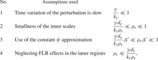
Table 1 gives a review of the assumptions that were adopted on the parameters during our the analysis. The assumption number 1 indicates a slow time variation of the perturbation. The assumption number 2 is the assumption on the scales of the inner region, where electron inertia becomes important and allows the break of the frozen flux condition. The assumption number 3 allows the use of the so-called constant $\psi$ approximation, implying that the dispersion relation is valid for large wavenumbers (Furth et al. Reference Furth, Killeen and Rosenbluth1963). The condition 4, imposed to neglect electron FLR, can be verified for a low-$\beta _e$ plasma. From a technical point of view, our new dispersion relation is obtained by solving the equations in the inner layer in real space, unlike in Porcelli (Reference Porcelli1991) where the corresponding equations are transformed and solved in Fourier space. The result of our linear theory, which is described in more detail in Appendix A, is given by the dispersion relation,

(3.9)\begin{equation} \gamma = 2 k_y \frac{d_e \rho_s}{{\rm \pi} \lambda} \varDelta' + \frac{\gamma^2 d_e {\rm \pi}\lambda}{4 k_y \rho_s^2}. \end{equation}

The first term on the right-hand side of (3.9) is exactly that of the formula (3.8), for $\lambda =1$. In the parameter regime indicated by table 1, the second term in (3.9) is a small term that provides a correction to the formula (3.8).

Table 1.

Table summarizing the various assumptions.

A solution of the dispersion relation (3.9), considered in the regime identified by the assumptions of table 1, is

(3.10)\begin{equation} \gamma_u = 2 k_y \left( \frac{ \rho_s ^2}{{\rm \pi} d_e \lambda }-\frac{\rho_s^{3/2}\sqrt{\rho_s - 2 d_e^2 \varDelta'}}{{\rm \pi} d_e \lambda } \right), \end{equation}

and is real for $\rho _s > 2 d_e^2 \varDelta '$. This new dispersion relation is tested against numerical simulations and compared with the expression (3.8). The numerical solver is pseudospectral and is based on a third-order Adams–Bashforth scheme. The scheme uses numerical filters acting on typical length scales much smaller than the physical scales of the system (Lele Reference Lele1992). The instability is triggered by perturbing the equilibrium with a disturbance of the parallel electron gyrocentre velocity field. Because of the requirement of periodic boundary conditions, the equilibrium (3.4a,b) is approximated by

(3.11)\begin{equation} A_{{\parallel}}^{(0)} (x)=\sum^{30}_{n={-}30} a_n {\rm e}^{{\rm i} n x}, \end{equation}

where $a_n$ are the Fourier coefficients of the function $f(x)= \lambda /\cosh ({x}/{\lambda } )^2$ (Grasso et al. Reference Grasso, Margheriti, Porcelli and Tebaldi2006). The numerical growth rate is determined by the formula

(3.12)\begin{equation} \gamma_N = \frac{{\rm d}}{{\rm d}t} \log\left| A_{{\parallel}}^{(1)} \left(\frac{\rm \pi}{2},0,t \right) \right|, \end{equation}

so that $A_\parallel ^{(1)}$ is evaluated at the X point, where reconnection takes place.

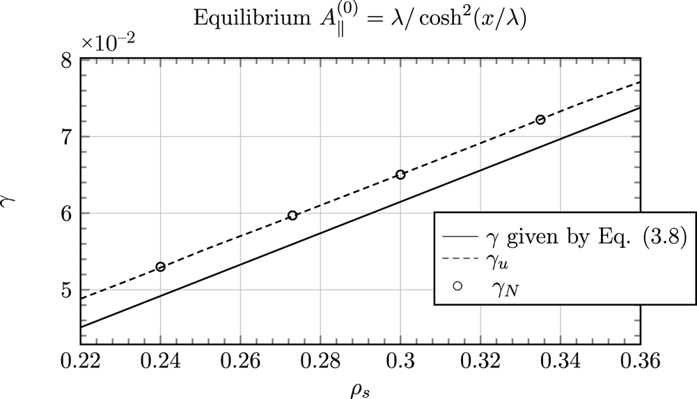
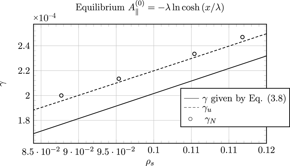
As shown on figures 1 and 2, the agreement between the theoretical and the numerical values appears to be improved by this new formula, when the latter is applied in its regime of validity. We also performed additional tests on a different equilibrium (the Harris sheet), as shown in figure 2. Also in this case, we observe that our new dispersion relation provides a better agreement with the numerical values. Consequently, (3.10) can be seen as an upgrade of the formula (3.8) in the regime of parameters indicated by table 1.

Figure 1.

Comparison between the analytical growth rate $\gamma _u$ obtained from the new formula (3.10) (dashed line), the analytical growth rate obtained from the formula (3.8) (solid line) and the numerical growth rate $\gamma _N$ defined in (3.12) (circles). The parameters are $d_e=0.1$, $\lambda =1$, $\varDelta '=0.72$, $m=1$. The box size is given by $- 10{\rm \pi} < x < 10{\rm \pi}$, $- 0.48{\rm \pi} < y < 0.48{\rm \pi}$. The values of the parameters lie in the regime of validity of the new formula (3.10). One can see that, for different values of $\rho _s$, the correction present in (3.10) yields a better agreement with the numerical values.

Figure 2.

This plot is showing additional tests, analogous to those of figure 1, but with the Harris sheet equilibrium $A_{\parallel }^{(0)} (x)= - \lambda \ln \cosh (x/\lambda )$ and $\phi ^{(0)}(x) = 0$, for which $\varDelta ^{'}_{H} =2( 1/(k_y \lambda ) - k_y \lambda )/\lambda$ and using the mode $m=1$. The parameters are $d_e=0.2$ and $\lambda =3$. The box size is $- 10{\rm \pi} < x < 10{\rm \pi}$, $- 4{\rm \pi} < y < 4{\rm \pi}$. For this case, $\varDelta '_{H}=0.38$. For this equilibrium the dispersion relation corresponds to $\gamma _{u} = k_y ( \rho _s ^2/({\rm \pi} d_e \lambda )- \rho _s^{3/2}(\rho _s - 2 d_e^2 \varDelta ^{'}_{H})^{1/2}/({\rm \pi} d_e \lambda ))$ and differs from (3.10) by a factor $2$ coming from the evaluation of $\textrm {d} B_{y0} /{\textrm {d} x}$ at the X point. Symbols are the same as in figure 1. Also in this case, the new formula yields a better agreement with the numerical values.

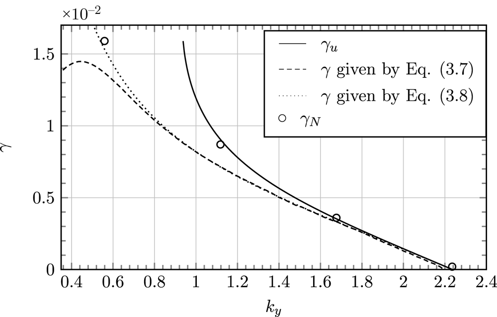
Figure 3 gives a comparison between the theoretical growth rate predicted by (3.7), (3.8) and (3.10), and the numerical growth rate $\gamma _N$ as a function of the wavenumber $k_y$. According to these tests, $\gamma _u$ seems to give a very good prediction for wavenumbers $k_y > 1.1$. The discrepancy observed for lower values of $k_y$ comes from the fact that the condition allowing the use of the constant $\psi$ approximation, $\varDelta ' \gamma d_e/ (k_y \rho _s)\ll \rho _s \varDelta ' \ll 1$, is no longer satisfied for a small wavenumber. The breakdown of $\gamma _u$ for $k_y \ll 0.95$ is due to the fact that for $\varDelta ' > \rho _s/(2 d_e^2)$, the solution (3.10) is no longer real.

Figure 3.

Comparison between the theoretical growth rate predicted by (3.7), (3.8) and (3.10), and the numerical growth rate $\gamma _N$ as a function of the wavenumber, $k_y={\rm \pi} m /L_y$. The parameters are $d_e=0.03$, $\rho _s=0.03$, $\lambda =1$. The runs were done with the modes $1 \leq m \leq 4$ and $L_y=1.789 {\rm \pi}$. The corresponding values of the tearing stability parameter lie in the interval $0.005 \leq \varDelta ' \leq 47.86$.

3.2. Numerical results for $\beta _e \ne 0$

We now proceed to a numerical study of the model (2.35) and (2.36), complemented by (2.37), (2.38) and (2.39). This will allow us to take into account the effects of finite $\beta _e$.

The numerical set-ups are the same as those presented in the previous section, relative to the equilibrium (3.4a,b), but the code accounts now for finite $\beta _e$ effects. The gyroaverage operators are introduced as they are defined in the Fourier space by (2.14) and (2.15). For the linear tests we focus on a weakly unstable regime for which $0<\varDelta '<1$. The strongly unstable case shows interesting behaviours in the nonlinear phase and will be studied in the next section. For all the tests, we will use $\lambda =1$. In order to isolate the contribution coming from purely varying $\beta _e$, we first scan $\beta _e$ from $10^{-3}$ to $1$ while $\rho _s$ and $d_e$ remain fixed, which is equivalent to considering a different mass ratio for each $\beta _e$ value. We recall that the parameters are indeed linked by the relations

(3.13)\begin{equation} \rho_e = \rho_s \sqrt{\frac{m_e}{m_i}} = d_e \sqrt{\frac{\beta_e}{2}}. \end{equation}

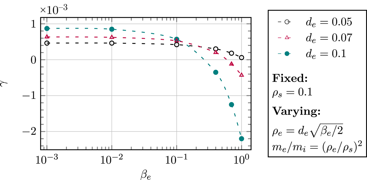
We repeat this scan for three different values of $d_e$. The results are presented in figure 4 and show that the effect of increasing $\beta _e$ and $m_e/m_i$ is stabilizing the tearing mode. This is consistent with the results obtained in the gyrokinetic and collisional study of Numata et al. (Reference Numata, Dorland, Howes, Loureiro, Rogers and Tatsuno2011), where $\beta _e$ and the mass ratio are also varied. Figure 4 also shows the competition between the destabilizing effect of the electron inertia and the stabilizing effect of $\beta _e$. For this set of parameters, the influence of $\beta _e$ on the weakly unstable regimes is almost negligible until $\beta _e=1$. For relatively low values of $\beta _e$, the highest growth rate corresponds to that for which the parameter $d_e$ is the largest. We recall in fact, from § 3.1, that, for $\beta _e \ll 1$, the formulae (3.8) and (3.10) hold. Such formulae, for $d_e \ll 1$, predict that the growth rate increases linearly with $d_e$. Conversely, when $\beta _e$ becomes large enough, as appears for $\beta _e > 0.15$, the growth rate for which $d_e$ is the largest, decreases drastically under the effect of the finite $\rho _e$ and of the parallel magnetic perturbations induced by $\beta _e$.

Figure 4.

Numerical growth rates of the collisionless tearing mode as a function of $\beta _e$, for three different values of $d_e$. The box length along $y$ is such that $-0.45{\rm \pi} < y<0.45 {\rm \pi}$, yielding a value of the tearing instability parameter of $\varDelta '=0.067$ for the largest mode in the system. We stand in a very small $\varDelta '$ regime, close to a marginal stability when $\beta _e < 0.1$. One sees that for higher values of $\beta _e$, and depending on the value of $d_e$, the mode is stabilized.

Some information about the stabilizing role of $\beta _e$ can be inferred by taking the small FLR limit of (2.36), which consists of considering the regime of parameters

(3.14a–c)\begin{equation} d_e \ll 1 , \quad \rho_s \ll 1 , \quad \frac{d_e}{\rho_s} \ll 1, \quad \beta_e = O(1), \end{equation}

and assuming

(3.15)\begin{equation} \nabla_{{\perp}}^2 = O(1). \end{equation}

If we retain the first-order FLR corrections as $d_e ,\rho _s \rightarrow 0$, the resulting Ohm's law reads

(3.16)\begin{align} & \frac{\partial}{\partial t}\left( A_{{\parallel}} +\left(\frac{\beta_e}{4}-1\right) d_e^2 \nabla_{{\perp}}^2 A_{{\parallel}} \right)+\left[ \phi , A_{{\parallel}} +\left(\frac{\beta_e}{4}-1\right) d_e^2 \nabla_{{\perp}}^2 A_{{\parallel}} \right] \nonumber\\ & \quad + \rho_s^2\left(\frac{\beta_e}{2 + \beta_e} -1\right)[\nabla_{{\perp}}^2 \phi , A_{{\parallel}}]=0. \end{align}

The new contributions in (3.16) are those due to finite $\beta _e$ and are not present in the usual two-field model by Schep et al. (Reference Schep, Pegoraro and Kuvshinov1994). In particular, the contributions proportional to $(\beta _e/4)d_e^2$ come from electron FLR effects and the contribution proportional to $\beta _e\rho _s^2/(2+\beta _e)$ is due to the presence of the finite $B_\parallel$. In (3.16), comparing with (3.2)–(3.3), it is possible to identify an effective electron skin depth $d_e'$ and an effective sonic Larmor radius $\rho _s'$, given by

(3.17)\begin{equation} \frac{d_e'}{d_e} = \sqrt{1 - \frac{\beta_e}{4}} \end{equation}

and

(3.18)\begin{equation} \frac{\rho_s '}{\rho_s}=\sqrt{\frac{2}{\beta_e +2}}, \end{equation}

respectively. This argument holds for $d_e '$ purely real and consequently for $\beta _e <4$. Because $d_e ' < d_e$, one can infer that the contribution of $\beta _e$, at the leading order in the expansion (3.14a–d)–(3.15), reduces the amplitude of the term that breaks the frozen-in condition. For this reason, one could indeed expect a stabilizing role of $\beta _e$. Deriving rigorously a dispersion relation for tearing modes from the model (2.35)–(2.39), in the general case with finite $\beta _e$, is a very challenging task. In the absence of a rigorous dispersion relation for finite $\beta _e$, a rough but readily available approximation can be obtained from the $\beta _e=0$ dispersion relation (3.10) (or (3.8)), replacing $d_e$ and $\rho _s$ with the effective parameters $d_e'$ and $\rho _s'$, respectively. This amounts to taking into account the leading-order electron FLR corrections, according to the ordering (3.14a–d)–(3.15), in Ohm's law, while neglecting all the $\beta _e$ effects in the electron continuity equation. In particular, higher-order derivative terms (coming from the gyroaverage operators, assuming it is possible to identify the multiplication operator for $k_x$ with $\partial _x$) are neglected, although these can become relevant around the resonant surface and thus influence the growth rate. Using this approximation, it follows immediately that the inclusion of finite $\beta _e$ corrections reduces the growth rate, given that $\gamma \propto d_e ' \rho _s '$ (if one considers the leading-order relation given by (3.8)) and that $d_e ' < d_e$ and $\rho _s ' < \rho _s$. However, the error made with this approximation needs to be checked numerically. We carried out this check by first determining the approximated growth rate in the following way. When replacing $d_e$ and $\rho _s$ by the effective $d_e'$ and $\rho _s'$ in our formula (3.10), valid for small $\varDelta '$, we obtain the dispersion relation

(3.19)\begin{equation} \gamma_{appr} =\dfrac{k_y \left(8 \rho_s^2-(\beta_e +2) \left(\dfrac{8\rho_s ^2}{\beta_e +2}\right)^{3/4}\sqrt{\sqrt{\dfrac{8 \rho_s ^2}{\beta_e +2}}+(\beta_e -4) \varDelta' d_e^2}\right)}{{\rm \pi} \sqrt{4-\beta_e } (\beta_e +2) d_e \lambda }. \end{equation}

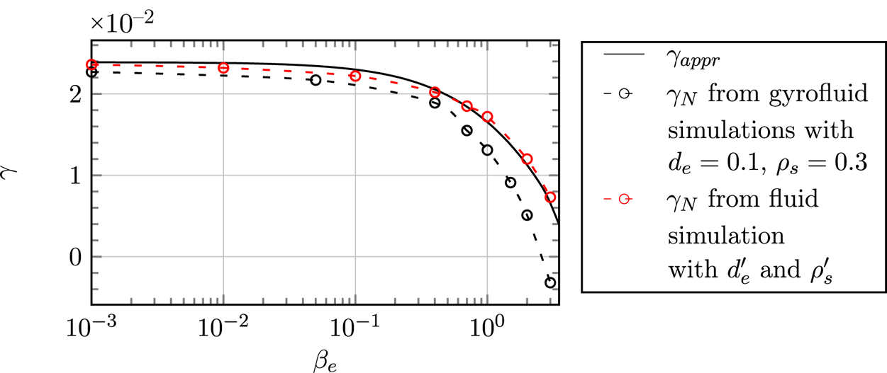
We tested the dispersion relation (3.19) against small $\varDelta '$ simulations and the results are shown on figure 5. By comparing the analytical formula (3.19) (solid black curve) and the numerical results obtained by the gyrofluid code (black circles), we can see that $\gamma _{appr}$ gives a reasonably good approximation for low $\beta _e$ values, as expected. The red circles in figure 5 show the growth rate obtained using, as input in the fluid code, the effective $d_e '$ and $\rho _s'$, that were calculated on the basis of the values $d_e= 0.1$ and $\rho _s = 0.3$ that we used in the gyrofluid code. The numerical and analytical growth rates obtained from the fluid model replacing $d_e$ and $\rho _s$ with the effective parameters, exhibit a behaviour qualitatively similar to that of the gyrofluid growth rate. However, a significant quantitative difference emerges as $\beta _e$ increases. This is due to the electron FLR contributions that are absent in the approximation. From figure 5 it emerges that the net effect of such contributions is that of further reducing the growth rate, as the curve obtained from the gyrofluid model always lies below those obtained from the effective fluid model.

Figure 5.

Numerical growth rates of the collisionless tearing mode as a function of $\beta _e$. The parameters are $d_e=0.1$, $\rho _s=0.3$, $\varDelta '=0.59$, $m=1$, $k_y=2.12$, $\lambda =1$. The solid black curve shows the approximate-$\beta _e$ dispersion relation (3.19). The black circles show the results obtained with the gyrofluid code. The red circles show the results obtained with the fluid code, using, instead of $d_e$ and $\rho _s$, $d_e'$ and $\rho _s'$, given by (3.17)–(3.18).

A further analysis we carried out consists of investigating the effect of $\beta _e$ on the linear growth rate, but at a fixed mass ratio. Physically, this might be interpreted as investigating the effect of the variation of the equilibrium electron temperature $T_{0e}$, supposing that $n_0$, $B_0$, $m_i$, $L$ (and thus the Alfvén frequency, which is the unit of measure of the dimensional growth rate) are fixed. 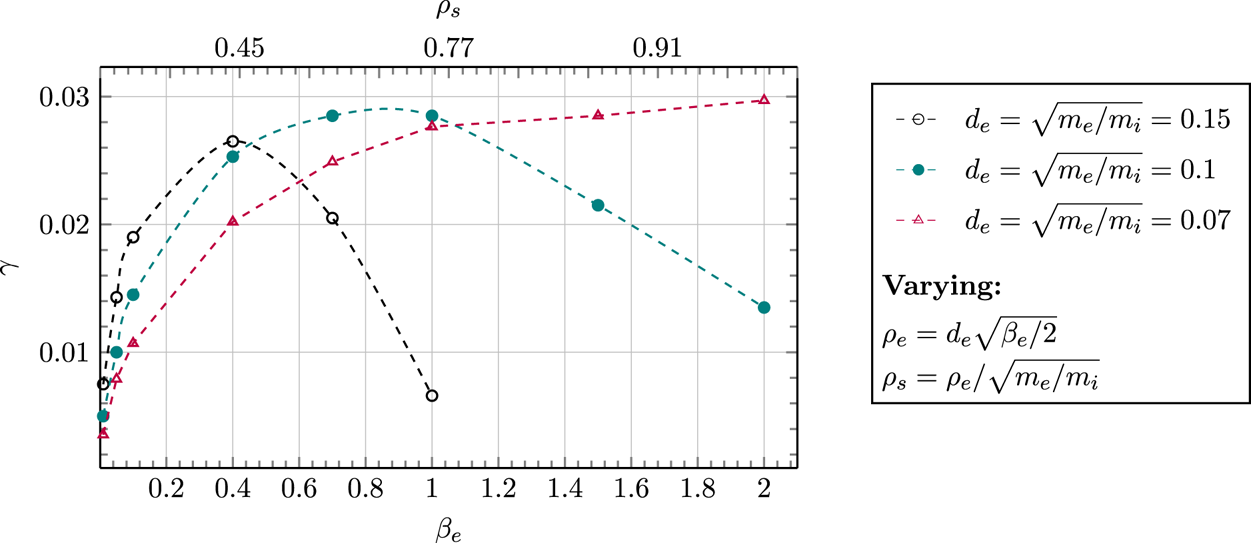In order to keep a constant mass ratio during the scan in $\beta _e$, we carried out a study with $\beta _e$ ranging from $10^{-3}$ to $2$ with $\rho _s$ varying simultaneously. We fix the relation $d_e = \sqrt {m_e/m_i}$ (implying $\rho _s=\sqrt {\beta _e / 2}$) and we evaluate the cases $d_e =$ 0.07, $d_e =$ 0.15, $d_e =$ 0.1. Figure 6 shows that when $\beta _e$ and $\rho _s$ are increased simultaneously there seems to be a competition between the destabilizing effect of $\rho _s$ and the stabilizing effect of $\beta _e$. Also in this case, the behaviour at small $\beta _e$, can be interpreted on the basis of the formulae (3.8) and (3.10), predicting an increase of the growth rate with increasing $\rho _s$. When electron FLR effects come into play at larger $\beta _e$, the growth rates decreases. The values chosen for the mass ratio in figure 6 are not realistic. Such values were chosen to show the dependence on the $\beta _e$ parameter more clearly. On the other hand, the mass ratio is not taken as a small parameter in the derivation of the model, so these values are respecting the validity conditions of the model. In the case of the artificial value of $d_e= \sqrt {m_e/m_i} = 0.15$, the stabilizing effect takes over the destabilizing effect of $\rho _s$ even for $\beta _e <1$. However, for the case $\sqrt {m_e/m_i} = 0.07$, much closer to a real mass ratio, the effect of $\rho _s$ appears to be dominant. Indeed, decreasing $d_e$ at a fixed $\beta _e$ amounts to decreasing $\rho _e$. Thus, for $d_e =0.07$ the stabilizing effect of the electron FLR terms gets weakened, with respect to the other values of $d_e$, even at large $\beta _e$.

Figure 6.

Numerical growth rates of the collisionless tearing mode as a function of $\beta _e$ and $\rho _s$, for different values of $d_e= \sqrt {m_e/m_i}$. The box size is $- {\rm \pi}< x < {\rm \pi}$, $- 0.47{\rm \pi} < y < 0.47{\rm \pi}$, which leads to $\varDelta '=0.59$.

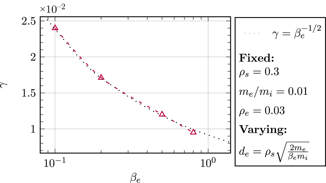
Figure 7 shows the variation of the growth rate of the tearing instability as a function of $\beta _e$, for a fixed value of $\rho _s = 10 \rho _e = 0.3$. The obtained results are confirming that the scaling of the growth rate as $\beta _e^{-1/2}$ (or, equivalently, as $d_e$) has been determined with the gyrokinetic study of Numata & Loureiro (Reference Numata and Loureiro2015). This shows the capability of the gyrofluid model to reasonably reproduce gyrokinetic results (Numata et al. Reference Numata, Dorland, Howes, Loureiro, Rogers and Tatsuno2011; Numata & Loureiro Reference Numata and Loureiro2015) and the fluid theory of Fitzpatrick & Porcelli (Reference Fitzpatrick and Porcelli2007), in a quantitative way.

Figure 7.

The value of $d_e$ for each run increases as $d_e=\rho _s\sqrt {2 m_e /(\beta _e m_i)}$. The box size is $- {\rm \pi}< x <{\rm \pi}$, $- 0.47{\rm \pi} < y < 0.47{\rm \pi}$. The numerical values (triangles) are compared with the curve $\gamma =\beta _e^{-1/2}$ (dotted line), which is the scaling predicted by Fitzpatrick & Porcelli (Reference Fitzpatrick and Porcelli2007) on the basis of a fluid model, and confirmed by gyrokinetic simulations by Numata et al. (Reference Numata, Dorland, Howes, Loureiro, Rogers and Tatsuno2011). The comparison shows that also our gyrofluid model confirms such a scaling.

3.2.1. Hot-ion limit, $\tau _i \rightarrow +\infty$

In this article we have focused, so far, on the cold-ion limit, but in this subsection we temporarily deviate from the cold-ion case, to consider the opposite limit, in which $\tau _i=\tau _{\perp i} \rightarrow +\infty$. The sole purpose of this subsection is to have a consistent and concise comparison of these two regimes, therefore we will only study the linear behaviour of the hot-ion limit and leave the study of its nonlinear evolution for a future work. The hot-ion limit can actually be of greater interest for space plasmas such as the solar wind. The ion gyrocentre density fluctuation and the ion gyrocentre parallel velocity are still neglected, and therefore the evolution equations remain unchanged. Only the assumption (2.25) is taken in the opposed limit, which has an impact on the development of ion gyroaverage operators. The static relations (2.37) and (2.39) are thus changed to

(3.20)\begin{gather} \phi = \frac{\rho_s^2 N_e}{\left(1 - \dfrac{\beta_e}{2}\right)G_{10e}-G_{10e}^{{-}1} }, \end{gather}

(3.21)\begin{gather}B_\parallel{=} \frac{\beta_e}{2 \rho_s^2} \phi. \end{gather}

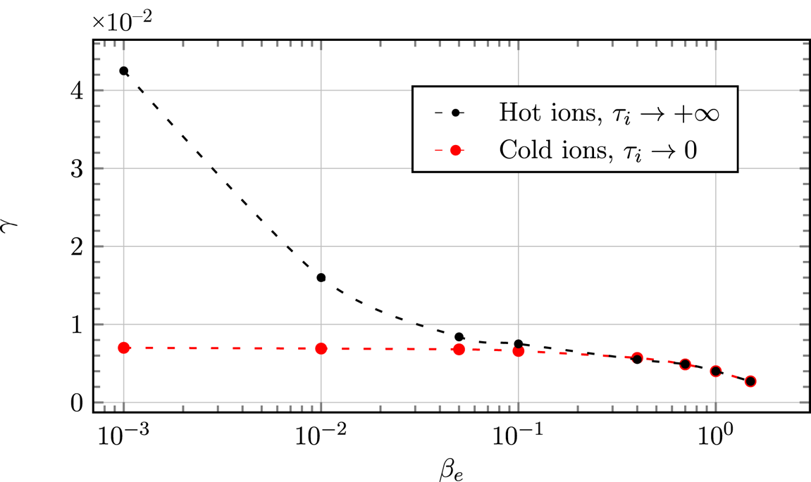
The linear results obtained in the hot-ion limit are compared with the results obtained in the cold-ion regime on figure 8. The parameters are $d_e=0.1$, $\rho _s=0.1$. Our results seem to indicate that, for $\beta _e> 0.5$, the growth rate is very insensitive to the temperature of the ions, which is in agreement with the results obtained by Numata et al. (Reference Numata, Dorland, Howes, Loureiro, Rogers and Tatsuno2011). Studies have been carried out with arbitrary ratio between the equilibrium ion and electron temperature in the low-$\beta$ limit, by Porcelli (Reference Porcelli1991) and Grasso et al. (Reference Grasso, Pegoraro, Porcelli and Califano1999), and predict that the growth rate is significantly higher when the temperature of the ion background temperature is higher than that of the electrons. This is indeed what we observe for $\beta _e<10^{-2}$.

Figure 8.

Comparison between the linear growth rate obtained in the cold-ion regime and the hot-ion regime. The box size is $- {\rm \pi}< x <{\rm \pi}$, $- 0.47{\rm \pi} < y < 0.47{\rm \pi}$, which leads to $\varDelta '=0.59$.

4. Nonlinear phase

To study the impact of a finite $\beta _e$ on the nonlinear evolution of the magnetic island, we focus on the strongly unstable case, $\varDelta '=14.31$ ($m=1$), resulting from a box length along $y$ given by $- {\rm \pi}< y < {\rm \pi}$. In this case, the mode $m=2$ has a positive tearing parameter $\varDelta '_{2} = 1.23$. The higher harmonics are linearly stable. The box along $x$ is chosen to be $-1.5 {\rm \pi}< x < 1.5 {\rm \pi}$ and allows us to reach a large island without incurring boundary effects. We make use of a resolution up to $2880\times 2880$ grid points. The mass ratio will be taken as $m_e/m_i = 0.01$ for the following tests.

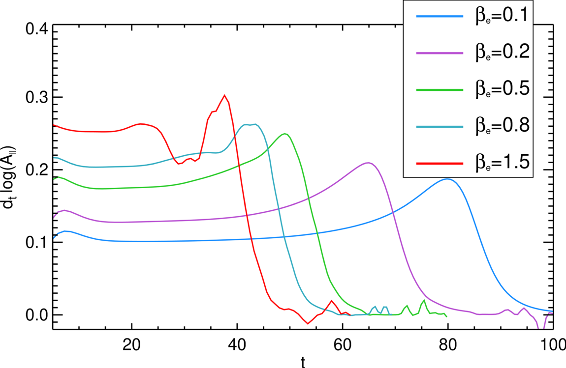
The first tests are carried out by making a scan in $\beta _e$ from $\beta _e = 0.1$ to $\beta _e=1.5$ while keeping $d_e = 0.08$ and varying $\rho _s$ as $\rho _s=0.8 \sqrt {\beta _e} /\sqrt {2}$. Increasing $\beta _e$ and $\rho _s$ simultaneously in this way, as stated in § 3.2, amounts to varying the electron background temperature $T_{0e}$. Figure 9 shows the evolution in time of the effective growth rate, given by (3.12), for each simulation. In all these cases, with the exception of $\beta _e=1.5$, we identify three phases: (1) a linear phase during which the perturbation evolution scales as $\exp (\gamma t)$; (2) a faster than exponential phase, which is delayed in the case $\beta _e=0.1$, given that the linear growth rate is smaller, with respect to the case $\beta _e=0.8$ for which the instability reaches the nonlinear phase faster; (3) a saturation during which the growth rate drops to $0$. We point out that, the fact that the linear growth rate increases with increasing $\beta _e$ is related to the fact that $\rho _s$ is also increased for each run. As discussed in the previous section, the isolated effect of an increasing $\beta _e$ in the equations actually implies a stabilization of the linear growth rate. In the case $\beta _e = 0.8$, the nonlinear growth shows a slightly different behaviour from the cases $\beta _e \leq 0.5$ and exhibits a stall phase, during which the growth rate slows down. This stall phase seems to separate two faster than exponential phases. Similar stall phases have been studied in Comisso et al. (Reference Comisso, Grasso, Waelbroeck and Borgogno2013), where a finite ion Larmor radius is considered, and appear to be obtained when considering a large ion Larmor radius. For the case $\beta _e = 1.5$, that we will focus on later, this slowdown is enhanced. We focus now on the case $\beta _e=0.8$. 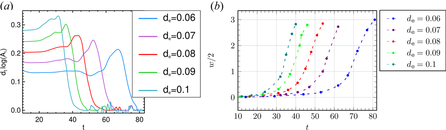We scan the values of $d_e$ from $0.06$ to $0.1$, and $\rho _s = 10\rho _e = 10 \sqrt {0.4} d_e \approx 6.32 d_e$. The results are shown in figure 10. These curves are compared for a fixed time unit (fixed $v_A$), while keeping $\beta _e$ and the mass ratio constant, which corresponds to varying $B_0 \sim n_0^{1/2}$ while keeping the electron temperature $T_{0e}$ fixed. For the case of $d_e= 0.06$, which corresponds to $\rho _s \sim 0.37$, we observe the slowdown at the end of the linear phase and it is followed by the faster than exponential phase. On the other hand, in the case of $d_e= 0.1$, for which $\rho _s \sim 0.63$, the slowdown appears at a later stage of the evolution process and seems to interrupt the faster than exponential phase by introducing a stall phase. We conclude that the effects of $\beta _e$, and consequently the effects of electron gyrations, causes the appearance of a slowing down phase of the growth of the island during the nonlinear evolution. The larger $\beta _e$, the more distinguishable this slowing phase will be. For a fixed values of $\beta _e$ and $m_e/m_i$, the fact of increasing $d_e$ and $\rho _s$, and consequently increasing the radius of gyration of the electrons, will delay the appearance of this slowing phase.

Figure 9.

Plot of the effective growth rate $({\textrm {d}}/{\textrm {d}t}) \log | A_{\parallel }^{(1)} ({{\rm \pi} }/{2},0,t ) |$, as a function of time. The corresponding values of $\beta _e$ are shown in the table. The value of the electron skin depth is kept fixed to $d_e=0.08$, whereas $\rho _s$ is varied (and ranges from $0.17$ to $0.69$) so to keep the mass ratio fixed to $m_e/m_i=0.01$. All the growth rates, except for the case $\beta _e=1.5$ exhibit the same behaviour, characterized by a linear, faster than exponential and saturation phase. The case $\beta _e=1.5$ exhibits also a slowdown phase.

Figure 10.

(a) Plot of the effective growth rate $({\textrm {d}}/{\textrm {d}t}) \log | A_{\parallel }^{(1)} ({{\rm \pi} }/{2},0,t ) |$, as a function of time. The parameters are $\beta _e =0.8$, implying $\rho _e=\sqrt {0.4}d_e$ and $\rho _s =10 \sqrt {0.4}d_e$. (b) Evolution of half-width of the magnetic island until saturation. The simulations correspond to those in panel (a).

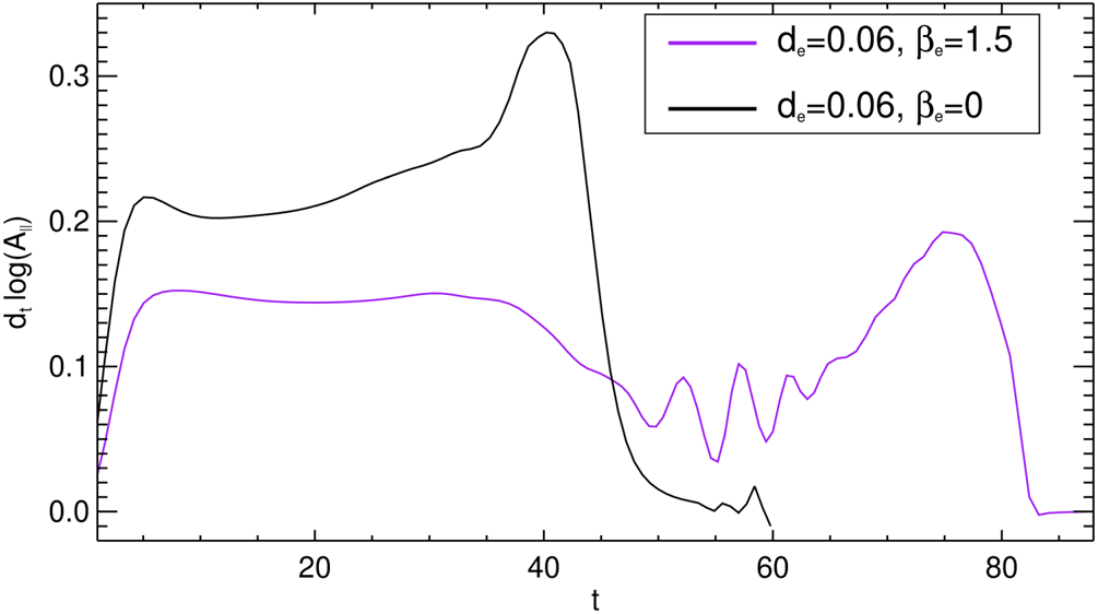
The evolution of the width of the magnetic island for these five runs is shown on the plot on the right-hand side of figure 10. The last point for each run corresponds to the half of the width of the island when the growth rate falls down to zero and enters the saturation phase. In conclusion, the reconnection time simply seems to be longer for smaller $d_e$, but the maximum width before saturation is identical for each case since the amount of initial magnetic energy is the same for each simulation. The last test consists of studying an extreme case for which the slowing down phase is accentuated, which corresponds to the case of $d_e= 0.06$, $\rho _s = 0.519$, $\beta _e = 1.5$. We also perform the simulation for $\beta _e=0$, using a code that solves the fluid equations (3.2)–(3.3). Figure 11 shows the overplot of the evolution of the growth rate for both simulations as a function of time. The slowing down phase is followed by an oscillation of the nonlinear growth rate. This oscillation was obtained in other tests for which $\beta _e = 1.5$.

Figure 11.

Plot of the effective growth rate $({\textrm {d}}/{\textrm {d}t}) \log | A_{\parallel }^{(1)} ({{\rm \pi} }/{2},0,t ) |$, for the cases $\beta _e=0$ (black curve) and $\beta _e=1.5$ (purple curve). The other parameters are $\rho _s = 0.519$ and $d_e=0.06$.

In order to understand in detail what causes this slowing down and these oscillations of the island growth that we observe between $t = 43$ and $t = 65$, we compared all the fields for the cases $\beta _e = 0$ and $\beta _e = 1.5$ of figure 11. 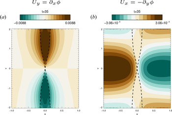A remarkable difference between these two regimes concerns the evolution of the inflow and outflow perpendicular velocities, given by $\boldsymbol {U}_{\perp }= \hat {z} \times \boldsymbol {\nabla } \phi$ and $\boldsymbol {U}_{\perp }= \hat {z}\times \boldsymbol {\nabla } (G_{10e} \phi - \rho _s^2 2 G_{20e} B_\parallel )$, respectively. Figure 12 shows the contour of the components $U_x$ and $U_y$ of the advecting perpendicular velocity for $\beta _e=0$. These contours do not show the entire box so that we focus on the island region drawn with the dotted lines. As expected, the contour of $U_y$ shows an outflow leaving the X point and $U_x$ shows an inflow in the direction of the X point.

Figure 12.

Contour plot of the perpendicular velocity component for $\beta _e=0$ with (a) $U_y$ and (b) $U_x$. The parameters are the same as those in figure 11. The magnetic island edges are shown by the dotted lines. Not the entire domain is shown.

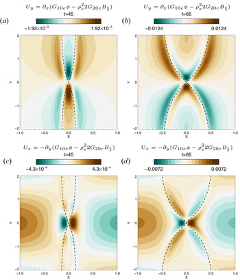
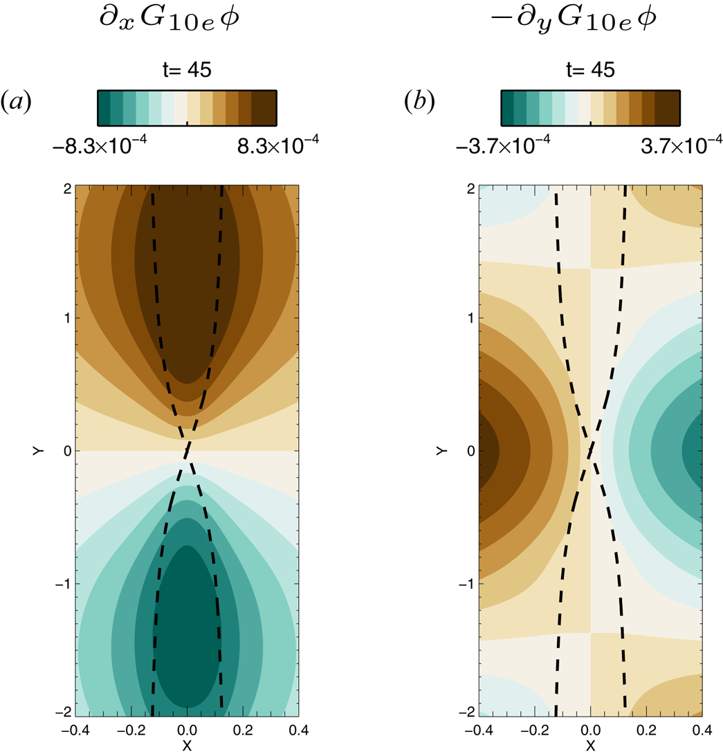
Figure 13 shows $U_x$ and $U_y$, for $\beta _e=1.5$, at two different times. For a better comparison we also show the part of the perpendicular velocity only induced by the electrostatic potential $\hat {z} \times \boldsymbol {\nabla } G_{10e} \phi$ on figure 14 to identify the role of $G_{10e} \phi$ and show that its behaviour in the case $\beta _e = 1.5$ is similar to that of the case $\beta _e = 0$. The first time shown in figure 13 corresponds to the beginning of the slowdown of the island growth. We observe that, close to the reconnection region, there is a small region where the velocity changes sign, with respect to the standard $\beta _e=0$ case. This inversion is more visible for $U_y$, where, inside the island, the fluid velocity is dominated by $B_\parallel$. We can conclude that $G_{10e} \phi \leq \rho _s^2 2 G_{20e} B_\parallel$ in the reconnected region. Consequently, the slowing down of the island growth can be explained by the fact that the advection velocity contains an additional drift due to the presence of the magnetic perturbation along the guide field. This effect decelerates the convergence of the field lines towards the reconnection region, where their evolution will be decoupled from that of the fluid. At the time $t=66$, when the island begins to grow faster than exponentially, the region where $G_{10e} \phi \leq \rho _s^2 2 G_{20e} B_\parallel$ shrinks and the advection towards the X point becomes much more effective, allowing the explosive growth.

Figure 13.

Here (a,b) $U_y$ and (c,d) $U_x$. For all these contours we used $\beta _e=1.5$ and the other parameters are the same as those in the figure 11. The magnetic island edges are shown by the dotted lines. Not the entire domain is shown.

Figure 14.

Contour plots of the components of the velocity field $\hat {z} \times \boldsymbol {\nabla } G_{10e} \phi$, at t=45. This corresponds to the case $\beta _e=1.5$ and the other parameters are the same as those in the figure 11. The magnetic island edges are shown by the dotted lines. Not the entire domain is shown.

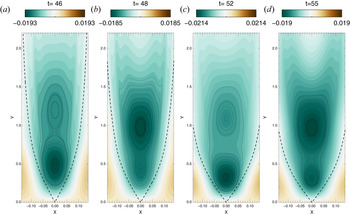
We now focus on the behaviour of $U_y$ during the small oscillations of the growth rate, visible on figure 11. Figure 15 shows a contour of $U_y$ in the upper part of the domain, between $t=46$ and $t=55$. The cell structures indicate two negative peaks. We recall that, in the case of $\beta _e=0$, we would observe a single positive peak. These peaks are growing at the centre of the island and will follow each other while moving toward the X point. The acceleration or deceleration of the island growth depends on the position (in absolute value) of the highest peak. When the highest peak is closer to the X point, the reconnection rate reaches a maximum ($t=46$ or $t=52$). This peak will then decrease while the other one, farther from the X point, will grow ($t=48$ or $t=55$). During this part of the cycle, the growth rate reaches a minimum. We interpret this intermittent flow, generated by the presence of $B_\parallel$, as the mechanism responsible for the accelerations and decelerations of the island growth.

Figure 15.

Contour plot of $U_y$ showing the upper part of the domain for $\beta _e=1.5$. The parameters are the same as those in figure 11. The magnetic island edges are shown by the dotted lines. Here $U_y$ is negative inside the island and the cell structures indicate the regions where the flow amplitude is greater. The situations where the highest (in absolute value) peak is closer to the X point ($t=46$ and $t=52$) correspond to maxima of the growth rate. Minima of the growth rate occur when the highest peak is far from the X point ($t=48$ and $t=55$).

4.1. Energy considerations

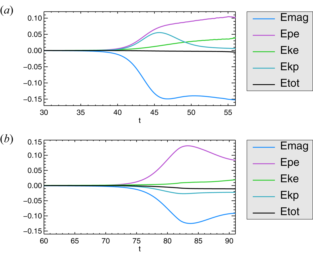
The time variations of the different components of the energy for the cases $\beta _e=0$ and $\beta _e=1.5$, whose growth rate is shown in figure 11, are shown on figure 16. The variations are defined as $(1/2)\int \,{\textrm {d}x}^2( \xi (x,y,t) - \xi (x,y,0)) / H(0)$ where the function $\xi$ can be replaced by the different contributions of the Hamiltonian (2.31). In terms of the gyrofluid variables and in the presence of FLR effects, identifying the physical meaning of all the contributions to the energy is not obvious. Therefore, we use the terminology adopted in Tassi et al. (Reference Tassi, Grasso, Borgogno, Passot and Sulem2018) and which refers to the fluid limit $\beta _e=0$. The different contributions are: the magnetic energy, $E_{\textrm {mag}}$, for which $\xi = - U_e G_{10e} A_{\parallel }$ (reduced to $|\boldsymbol {\nabla }_{\perp } A_{\parallel }|^2$ in the fluid case); the parallel electron kinetic energy, $E_{ke}$, for which $\xi = d_e^2 U_e^2$ (reduced to $d_e^2 ( \nabla _{\perp }^2 A_{\parallel })^2$ in the fluid case); the energy due to the fluctuation of the electron density, $E_{pe}$, for which $\xi = \rho _s^2 N_e^2$ (reduced to $\rho _s^2 (\boldsymbol {\nabla }_\perp ^2 \phi )^2$ in the fluid case); and the perpendicular electrostatic energy of the electrons combined with the energy of the parallel magnetic perturbations, $E_{kp}$, for which $\xi = - ( G_{10e} \phi - \rho _s^2 2 G_{20e} B_\parallel ) N_e$ (reduced to $|\boldsymbol {\nabla }_{\perp } \phi |^2$ in the fluid case). We consider the simulation as being reliable until the time at which the percentage of the total energy that gets dissipated numerically (black curve) reaches $1\,\%$.

Figure 16.

Time evolution of the energy variations for the cases $\beta _e=0$ (a) and $\beta _e=1.5$ (b). The parameters are $d_e=0.06$, $\rho _s=0.519$ and their corresponding growth rate is shown in figure 11.

By comparing the two simulations, one can see that there appears to be a comparable amount of magnetic energy being converted. The remarkable difference is the evolution of the component that combines the electrostatic energy and the energy of the parallel magnetic perturbations, $E_{kp}$, which, in the case $\beta _e=1.5$, also seems to be converted into electron thermal energy ($E_{pe}$), resulting in an increase in this component. This decrease of the electrostatic energy has been observed only in the case $\beta _e=1.5$. In the case of $\beta _e =0.8$, it appears that this component stays rather close to its initial value.

We also carried out the test with $\beta _e=1.5$ by artificially removing the parallel magnetic perturbation $B_\parallel$ from the code, and consequently it was not appearing in the expression of $E_{kp}$. It appeared first that the presence of $B_\parallel$ has a stabilizing effect on the tearing mode (which is consistent with the linear results discussed in § 3.2), and secondly, the energy component $E_{kp}$ was slightly increasing instead of decreasing. This allows us to conclude that the energy related to the parallel magnetic perturbations is in fact the decreasing component that seems to be converted into electron thermal energy $E_{pe}$.

5. Conservation laws of the model

In this section we discuss the conservation laws of the gyrofluid model and its Lagrangian invariants. Equations (2.35)–(2.36) can be recast in the form

(5.1)\begin{equation} \frac{\partial A_\pm}{\partial t}+\boldsymbol{v}_\pm \boldsymbol{\cdot} \boldsymbol{\nabla} A_\pm{=}0, \end{equation}

where

(5.2)\begin{gather} A_\pm{=} G_{10e} A_{{\parallel}} - d_e^2 U_e \pm d_e \rho_s N_e, \end{gather}

(5.3)\begin{gather}\boldsymbol{v}_\pm{=} \hat{z} \times \boldsymbol{\nabla} \left(G_{10e} \phi - \rho_s^2 2 G_{20e} B_\parallel{\pm} \frac{\rho_s}{d_e} G_{10e} A_{{\parallel}}\right). \end{gather}

We define by

(5.4)\begin{equation} \phi_\pm{=} G_{10e} \phi - \rho_s^2 2 G_{20e} B_\parallel{\pm} \frac{\rho_s}{d_e} G_{10e} A_{{\parallel}}, \end{equation}

the stream functions of the velocity fields $\boldsymbol {v}_\pm = \hat {z} \times \boldsymbol {\nabla } \phi _\pm$. The formulation (5.1) makes the presence of Lagrangian invariants evident, corresponding to the fields $A_\pm$, in the model. Such Lagrangian invariants are advected by the incompressible velocity fields $\boldsymbol {v}_\pm$. The presence of such Lagrangian invariants is a feature common to many 2-D Hamiltonian reduced gyrofluid models (Waelbroeck, Hazeltine & Morrison Reference Waelbroeck, Hazeltine and Morrison2009; Grasso et al. Reference Grasso, Tassi and Waelbroeck2010; Waelbroeck & Tassi Reference Waelbroeck and Tassi2012; Keramidas Charidakos, Waelbroeck & Morrison Reference Keramidas Charidakos, Waelbroeck and Morrison2015; Tassi Reference Tassi2017, Reference Tassi2019; Passot, Sulem & Tassi Reference Passot, Sulem and Tassi2018; Grasso & Tassi Reference Grasso and Tassi2015) and is related to the existence of infinite families of Casimir invariants of the Poisson bracket.

For (2.35)–(2.36), such invariants correspond to the two families

(5.5a,b)\begin{equation} C_+{=}\int \,{\rm d}^2 x \, \mathcal{C}_+ (A_+), \quad C_-{=}\int \,{\rm d}^2 x \, \mathcal{C}_- (A_-), \end{equation}

where $\mathcal {C}_\pm$ are arbitrary functions. Equations (5.1) imply that contour lines of the fields $A_\pm$ cannot reconnect, as the corresponding vector fields $\boldsymbol {B}_\pm =\boldsymbol {\nabla } A_\pm \times \hat {z}$ are frozen in the velocity fields $\boldsymbol {v}_\pm$. On the other hand, the same model allows magnetic field lines to reconnect. In particular, it is useful to illustrate the mechanisms breaking the frozen-in condition in this model. This can be done by inspection of (2.36), governing the evolution of $A_{\parallel }$ and, consequently, of the magnetic field in the plane perpendicular to the guide field, which is given by $\boldsymbol {B}_\perp =\boldsymbol {\nabla } A_{\parallel } \times \hat {z}$. Equation (2.4) can be rewritten in the following way:

(5.6)\begin{align} & \frac{\partial A_{{\parallel}}}{\partial t} + \boldsymbol{u} \boldsymbol{\cdot} \boldsymbol{\nabla} A_{{\parallel}} \nonumber\\ & \quad ={-}\frac{\mathcal{D}}{\mathcal{D} t} \left(\left( \frac{\beta_e}{4} -1\right) d_e^2 \nabla_{{\perp}}^2 A_{{\parallel}} + \sum_{n=2}^{+\infty} \left( \frac{\beta_e}{4n}-({-}1)^{n-1}\right)\left(\frac{\beta_e}{4}\right)^{n-1}\frac{(d_e^2 \nabla_{{\perp}}^2)^n}{(n-1) !} A_{{\parallel}} \right) \nonumber\\ & \qquad -\rho_s^2 \sum_{n=1}^{+\infty} \frac{1}{n!}\left( \frac{\beta_e}{4} d_e^2\right)^n [ {(\nabla_{{\perp}}^2)}^n A_{{\parallel}} , N_e], \end{align}

where

(5.7)\begin{equation} \boldsymbol{u}=\hat{z}\times\boldsymbol{\nabla}(G_{10e} \phi - \rho_s^2 2 G_{20e} B_\parallel{-} \rho_s^2 N_e), \end{equation}

and where the operator $\mathcal {D}/\mathcal {D} t$ is defined by

(5.8)\begin{equation} \frac{\mathcal{D}f}{\mathcal{D} t}=\frac{\partial f}{\partial t}+[G_{10e} \phi - \rho_s^2 2 G_{20e} B_\parallel ,f] \end{equation}

for a function $f$. In (5.6) we also used the formal expansions

(5.9a,b)\begin{equation} G_{10e}=\sum_{n=0}^{+\infty}\frac{1}{n!} \left(\frac{\beta_e}{4} d_e^2 \nabla_{{\perp}}^2 \right)^n, \quad G_{10e}^{{-}1}=\sum_{n=0}^{+\infty}\frac{({-}1)^n}{n!} \left(\frac{\beta_e}{4} d_e^2 \nabla_{{\perp}}^2 \right)^n. \end{equation}

The right-hand side of (5.6) contains all the terms that break the frozen-in condition. Indeed, if the right-hand side of (5.6) vanishes, the perpendicular magnetic field is frozen in the velocity field $\boldsymbol {u}$. From (5.6) one thus sees that the frozen-in condition can be violated by electron inertia (associated with the parameter $d_e$) and by electron FLR effects (associated with the combination $d_e^2 \beta _e /4$). In the limit $\beta _e=0$ only electron inertia remains to break the frozen-in condition. On the other hand, because electron FLR terms are associated with the product between $\beta _e/4$ and $d_e^2$, in the limit $d_e=0$ both electron inertia and electron FLR terms disappear and the right-hand side of (5.6) vanishes, thus restoring the frozen-in condition. We remark that the presence of a finite $\beta _e$ is also responsible for finite parallel magnetic perturbations $B_\parallel$. However, these do not violate the frozen-in condition for the perpendicular magnetic field, as they only contribute to modify the advecting velocity field $\boldsymbol {u}$ (the parallel magnetic field lines, on the other hand, might undergo reconnection).

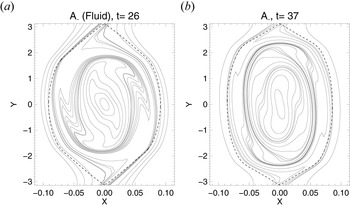
We consider here the qualitative structures of the contour plots of the Lagrangian invariants $A_\pm$ referring to the choice of parameters already adopted for figure 11. From comparing the contour plots of $A_{-}$, in the case $\beta _e=0$ (left-hand panel of figure 17) and $\beta _e=1.5$ (right-hand panel of figure 17), the structures look qualitatively similar. The contour lines of $A_{-}$ are induced by the velocity fields $\phi _{-}$ and undergo a phase mixing (the field $A_{+}$ is winding up identically in the opposite direction, induced by $\phi _{+}$). The duration of the transient and linear phases are not identical, consequently we compared the fields at the normalized time $\gamma t= 5.18$, which makes it possible to compare the fields when the islands are of comparable size so that they reached the same stage of evolution. The separatrices are displayed on each plot by dashed lines. We observe a different shape of the island in the two cases, which reflects the different distribution of the spectral power of the magnetic field. The effect of $\beta _e$ gives a more elongated island along $y$ and thinner along $x$. If we take a $\beta _e>1$ and keep a low enough mass ratio, then we are forced to stand in a regime with $\rho _s/d_e$ much greater than $1$. The ratio considered in this simulation is $\rho _s/d_e=8.65$. In this case $A_\pm$ is advected by a velocity field which can be approximated by $\boldsymbol {v}_\pm = \pm \hat {z} \times \boldsymbol {\nabla } (({\rho _s}/{d_e}) G_{10e} A_{\parallel })$, since $\phi _\pm$ tends to coincide with $\pm ({\rho _s}/{d_e}) G_{10e} A_{\parallel }$. Performing other tests (whose results are not shown here) with $d_e \sim \rho _s$, $\beta _e \in \{0, 0.5\}$ and a mass ratio $20$ times higher, did not show any obvious difference in the mixing phase either.

Figure 17.

Contour plot of the Lagrangian invariant $A_{-}$ with (a) $\beta _e=0$ and (b) $\beta _e=1.5$. The parameters are $d_e=0.06$, $\rho _s=0.519$. The dashed lines are the separatrices. The contour plots refer to the normalized time $\gamma t= 5.18$.

The electron density $N_e$ can be obtained by a linear combination of the invariants $A_\pm$:

(5.10)\begin{equation} N_e = \frac{A_+{-} A_-}{2 d_e \rho_s}. \end{equation}

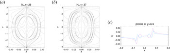
The contour plot of the electron density is displayed in figure 18 and shows the fine structures produced by the mixing of the Lagrangian invariants $A_\pm$. The case $\beta _e=1.5$ shows nested quadripolar structures. From the difference between the profiles of $N_e$ in figure 18 it is visible that increasing $\beta _e$ smoothes the gradients in the inner region of the electron density.

Figure 18.

Contour plot of the electron density with (a) $\beta _e=0$ and (b) $\beta _e=1.5$. Panel (c) are the profiles of $N_e$ at $y={\rm \pi} /3$ in the cases $\beta _e=0$ (purple) and $\beta _e=1.5$ (blue). The parameters are $d_e=0.06$, $\rho _s=0.519$. The dashed lines are the separatrices. The contour plots and profiles refer to the normalized time $\gamma t= 5.18$.