2.1 Typical self-similar systems

Before we prove our main result, Theorem 1.3, we show some applications of it. First, we show that the assumption $\max _{i\neq j}\{|r_i|+|r_j|\}<1$ in [Reference Bárány, Simon and Solomyak4, Corollary 6.8.12] can be strengthened.

Theorem 2.1. Let $\mathcal {I}=\{f_i(x)=r_ix+c_i\}_{i=1}^N$ be a self-similar IFS. Then there exists a set $\mathbf {E}\subset (0,1)^{N}$ with $\dim _{\mathrm {H}}(\mathbf {E})\leq N-1$ such that for every $(r_{i})_{i=1}^N\in (0,1)^{N}\setminus \mathbf {E}$ there exists a set $\mathbf {F}\subset \mathbb {R}^N$ with $\dim _{\mathrm {H}}(\mathbf {F})\leq N-1$ such that for every $(c_i)_{i=1}^N\in \mathbb {R}^N\setminus \mathbf {F}$ the following statement holds: for every self-similar measure $\mu $ corresponding to the self-similar IFS $\mathcal {I}$ and the probability vector $\mathbf {p}=(p_{i})_{i=1}^{N}$ ,

$$ \begin{align*}\dim_{\mathrm{H}}(\mu)=\min\bigg\{1, \frac{-\sum_{i=1}^{N}p_{i}\log(p_{i})}{-\sum_{i=1}^{N}p_{i}\log(r_{i})}\bigg\}.\end{align*} $$

2.2 Estimating $\Phi (\mathbf {p})$

We will now establish a bound for $\Phi (\mathbf {p})$ , which might help estimate from below the Hausdorff dimension of self-similar measures with common fixed-point structure.

Proposition 2.2. Let $\mathbf {p}=(p_{i,j})_{1\leq i\leq N, 1\leq j\leq n_i}$ be a probability vector and let $\Phi (\mathbf {p})$ be defined as in (1.4). Then

$$ \begin{align*}\Phi(\mathbf{p}) \geq \sum_{l=1}^{N}\sum_{m=1}^{n_{l}}p_{l,{m}} \log \bigg(p_{l,{m}}+\sum_{\substack{i\ne l\\ i=1}}^{N}\sum_{j=1}^{n_i}p_{i,j}\bigg).\end{align*} $$

Proof. Let us recall the representation of $\Phi (\mathbf {p})$ from §1. Suppose $X_{1},X_{2},\ldots $ are i.i.d. random variables such that $\mathbb {P}(X_r=(i,j))=p_{i,j}$ for all $i\in \{1,\ldots ,N\}$ and $j\in \{1,2,\ldots ,n_i\}$ . Let $k_{i,j}:=\min \{r\geq 1: X_r\notin \{(i,1),\ldots ,(i,n_i)\} \},$ and let $Y_{i,j}:=\#\{1\leq r\leq k_{i,j}-1: X_r=(i,j)\}$ for all $j\in \{1,2,\ldots ,n_i\}.$ Then the quantity $\Phi (\mathbf {p})$ can be written in the form

$$ \begin{align*} \Phi(\mathbf{p})= \mathbb{E}\bigg(\log\bigg(\frac{Y_{X_1}}{k_{X_1}-1}\bigg)\bigg)=\sum_{l=1}^{N}\sum_{m=1}^{n_{l}}p_{l,{m}} \mathbb{E}\bigg(\log\bigg(\frac{Y_{l,m}}{k_{l,m}-1}\bigg) \bigg| X_{1}=(l,m)\bigg),\end{align*} $$

where

$$ \begin{align*} &\mathbb{E}\bigg(\log\bigg(\frac{Y_{l,m}}{k_{l,m}-1}\bigg) \bigg| X_{1}=(l,m)\bigg)\\ &\quad= \sum_{k=0}^{\infty}\sum_{q=0}^{k}\binom{k}{q}p_{l,m}^q\bigg(\sum_{\substack{j=1\\j\neq m}}^{n_l}p_{l,j}\bigg)^{k-q}\bigg(1-\sum_{j=1}^{n_l}p_{l,j}\bigg)\log\bigg(\frac{q+1}{k+1}\bigg). \end{align*} $$

Clearly,

$$ \begin{align*} \mathbb{E}\bigg(\log\bigg(\frac{Y_{l,m}}{k_{l,m}-1}\bigg) \bigg| X_{1}=(l,m)\bigg)&=\mathbb{E}\bigg(-\log\bigg(\frac{k_{l,m}-1}{Y_{l,m}}\bigg) \bigg| X_{1}=(l,m)\bigg)\\ &\geq -\log \mathbb{E}\bigg(\frac{k_{l,m}-1}{Y_{l,m}} \bigg| X_{1}=(l,m)\bigg), \end{align*} $$

where we used Jensen’s inequality. Then

$$ \begin{align*} \mathbb{E}\bigg(\frac{k_{l,m}-1}{Y_{X_1}}| X_{1}=(l,m)\bigg)&=\sum_{k=0}^{\infty}\sum_{q=0}^{k}\binom{k}{q}p_{l,m}^q\bigg(\sum_{\substack{j=1\\j\neq m}}^{n_l}p_{l,j}\bigg)^{k-q}\bigg(1-\sum_{j=1}^{n_l}p_{l,j}\bigg)\frac{k+1}{q+1}\\&=\sum_{k=0}^{\infty}\sum_{q=0}^{k}\binom{k+1}{q+1}p_{l,m}^{q}\bigg(\sum_{\substack{j=1\\j\neq m}}^{n_l}p_{l,j}\bigg)^{k-q}\bigg(1-\sum_{j=1}^{n_l}p_{l,j}\bigg)\\&=\sum_{k=1}^{\infty}\bigg(1-\sum_{j=1}^{n_l}p_{l,j}\bigg)\frac{1}{p_{l,m}}\bigg(\bigg(\sum_{j=1}^{n_l}p_{l_j}\bigg)^{k}-\bigg(\sum_{\substack{j=1\\j\ne m}}^{n_l}p_{l_j}\bigg)^{k}\bigg)\\&=\bigg(\!1-\sum_{j=1}^{n_l}p_{l_j}\!\bigg)\frac{1}{p_{l,m}}\bigg(\!\frac{\sum_{j=1}^{n_l}p_{l,j}}{1-\sum_{j=1}^{n_l}p_{l,j}}-\frac{\sum_{j=1,j\ne m}^{n_l}p_{l,j}}{1-\sum_{j=1,j\ne m}^{n_l}p_{l,j}}\!\bigg)\\&=\bigg(1-\sum_{\substack{j=1\\j\ne m}}^{n_l}p_{l,j}\bigg)^{-1}=\bigg(p_{l,{m}}+\sum_{\substack{i\ne l\\ i=1}}^{N}\sum_{j=1}^{n_i}p_{i,j}\bigg)^{-1}. \end{align*} $$

Thus, from the above, we have

$$ \begin{align*}\mathbb{E}\bigg(\log\bigg(\frac{Y_{l,m}}{k_{l,m}-1}\bigg) \bigg| X_{1}=(l,m)\bigg)\geq \log \bigg(p_{l,{m}}+\sum_{\substack{i\ne l\\ i=1}}^{N}\sum_{j=1}^{n_i}p_{i,j}\bigg).\end{align*} $$

This implies that

$$ \begin{align*}\Phi(\mathbf{p}) \geq \sum_{l=1}^{N}\sum_{m=1}^{n_{l}}p_{l,{m}} \log \bigg(p_{l,{m}}+\sum_{\substack{i\ne l\\ i=1}}^{N}\sum_{j=1}^{n_i}p_{i,j}\bigg).\end{align*} $$

This completes the proof.

2.3 Generalized 4-corner set

Using Theorem 1.3, we can also calculate the Hausdorff dimension of self-affine measures supported on the generalized $4$ -corner set. Let

(2.1) $$ \begin{align} \begin{aligned} F_{1}(x,y)&=(\gamma_{1,1}x,\unicode{x3bb}_{1,1}y), F _{2}(x,y)=(\gamma_{1,2}x,\unicode{x3bb}_{2,1}y+(1-\unicode{x3bb}_{2,1})),\\F_{3}(x,y)&=(\gamma_{2,1}x+(1-\gamma_{2,1}),\unicode{x3bb}_{1,2}y), F_{4}(x,y)=(\gamma_{2,2}x+(1-\gamma_{2,2}),\unicode{x3bb}_{2,2}y\\ & \!\qquad +(1-\unicode{x3bb}_{2,2})) \end{aligned} \end{align} $$

be a self-affine IFS on $\mathbb {R}^2$ such that

(2.2) $$ \begin{align} \left.\begin{array}{c@{}} 0<\gamma_{i,j},\unicode{x3bb}_{i,j}\text{ for }i=1,2, j=1,2,\\ \gamma_{1,1}+\gamma_{2,1}\leq 1,\ \gamma_{1,2}+\gamma_{2,2}\leq 1,\ \unicode{x3bb}_{1,1}+\unicode{x3bb}_{2,1}\leq1,\ \unicode{x3bb}_{1,2}+\unicode{x3bb}_{2,2}\leq1,\\ \min\{\gamma_{1,2}+\gamma_{2,1},\unicode{x3bb}_{1,2}+\unicode{x3bb}_{2,1}\}\leq1\text{ and }\min\{\gamma_{1,1}+\gamma_{2,2},\unicode{x3bb}_{1,1}+\unicode{x3bb}_{2,2}\}\leq1. \end{array}\right\} \end{align} $$

The conditions in (2.2) guarantee that the IFS $\{F_1,F_2,F_3,F_4\}$ satisfies the rectangular OSC. In particular, $F_i((0,1)^2)\subset (0,1)^2$ and $F_i((0,1)^2)\cap F_j((0,1)^2)=\emptyset $ for every ${i\neq j\in \{1,2,3,4\}}$ . We call the attractor $C=\bigcup _{i=1}^4F_i(C)$ of $\{F_1,\ldots ,F_4\}$ the generalized 4-corner set. In [Reference Bárány3], the first author studied the box-counting dimension of the 4-corner set for Lebesgue typical parameters. We now determine the Hausdorff dimension of self-affine measures supported on C for typical parameters in a certain sense, and the Hausdorff dimension of the generalized 4-corner set in a region of parameters.

Let $\mathbf {p}=(p_1,\ldots ,p_4)$ be a probability vector, and let

$$ \begin{align*} \chi_x(\mathbf{p})&=-p_1\log\gamma_{1,1}-p_2\log\gamma_{1,2}-p_3\log\gamma_{2,1}-p_4\log\gamma_{2,2},\\ \chi_y(\mathbf{p})&=-p_1\log\unicode{x3bb}_{1,1}-p_2\log\unicode{x3bb}_{2,1}-p_3\log\unicode{x3bb}_{1,2}-p_4\log\unicode{x3bb}_{2,2}. \end{align*} $$

Theorem 2.3. Let $\{F_1,F_2,F_3,F_4\}$ be a self-affine IFS as in (2.1). There exist sets $\mathbf {E}_x,\mathbf {E}_y\subset (0,1)^{4}$ with $\dim _{\mathrm {H}}(\mathbf {E}_x),\dim _{\mathrm {H}}(\mathbf {E}_y)\leq 3$ such that for every $(\gamma _{i,j})_{i=1,j=1}^{2,2}\in (0,1)^{4}\setminus \mathbf {E}_x$ and $(\unicode{x3bb} _{i,j})_{i=1,j=1}^{2,2}\in (0,1)^{4}\setminus \mathbf {E}_y$ with (2.2) the following statement holds: for every self-affine measure $\mu $ corresponding to the IFS $\{F_1,F_2,F_3,F_4\}$ and the probability vector $\mathbf {p}=(p_{1},p_2,p_3,p_4)$ ,

$$ \begin{align*}\dim_{\mathrm{H}}(\mu)=\begin{cases} \dfrac{h_{\mathbf{p}}+\Phi_x(\mathbf{p})}{\chi_x(\mathbf{p})}-\dfrac{\Phi_x(\mathbf{p})}{\chi_y(\mathbf{p})} & \text{if }\chi_y(\mathbf{p})\geq\chi_x(\mathbf{p})\geq h_{\mathbf{p}}+\Phi_x(\mathbf{p}),\\[10pt] 1+\dfrac{h_{\mathbf{p}}-\chi_x(\mathbf{p})}{\chi_y(\mathbf{p})} & \text{if }\chi_y(\mathbf{p}),h_{\mathbf{p}}+\Phi_x(\mathbf{p})\geq\chi_x(\mathbf{p}), \\[10pt] \dfrac{h_{\mathbf{p}}+\Phi_y(\mathbf{p})}{\chi_y(\mathbf{p})}-\dfrac{\Phi_y(\mathbf{p})}{\chi_x(\mathbf{p})} & \text{if }\chi_x(\mathbf{p})\geq\chi_y(\mathbf{p})\geq h_{\mathbf{p}}+\Phi_y(\mathbf{p}),\\[10pt] 1+\dfrac{h_{\mathbf{p}}-\chi_y(\mathbf{p})}{\chi_x(\mathbf{p})} & \text{if }\chi_x(\mathbf{p}),h_{\mathbf{p}}+\Phi_y(\mathbf{p})\geq\chi_y(\mathbf{p}), \end{cases}\end{align*} $$

where

$$ \begin{align*} \Phi_x(\mathbf{p})&=\sum_{k=0}^{\infty}\sum\limits_{q=0}^{k}\binom{k}{q}(p_3+p_4)\bigg(p_{1}^{q+1}p_{2}^{k-q}+p_2^{q+1}p_1^{k-q}\bigg)\log\bigg(\frac{q+1}{k+1}\bigg)\\ &\quad+\sum_{k=0}^{\infty}\sum\limits_{q=0}^{k}\binom{k}{q}(p_1+p_2)\bigg(p_{3}^{q+1}p_{4}^{k-q}+p_4^{q+1}p_3^{k-q}\bigg)\log\bigg(\frac{q+1}{k+1}\bigg) \end{align*} $$

and

$$ \begin{align*} \Phi_y(\mathbf{p})&=\sum_{k=0}^{\infty}\sum\limits_{q=0}^{k}\binom{k}{q}(p_2+p_4)\bigg(p_{1}^{q+1}p_{3}^{k-q}+p_3^{q+1}p_1^{k-q}\bigg)\log\bigg(\frac{q+1}{k+1}\bigg)\\ &\quad+\sum_{k=0}^{\infty}\sum\limits_{q=0}^{k}\binom{k}{q}(p_1+p_3)\bigg(p_{2}^{q+1}p_{4}^{k-q}+p_4^{q+1}p_2^{k-q}\bigg)\log\bigg(\frac{q+1}{k+1}\bigg). \end{align*} $$

Example 2.4. Theorem 2.3 allows us to calculate the Hausdorff dimension of the generalized 4-corner set for Lebesgue typical points on a certain region of parameters. Let us further suppose that

(2.3) $$ \begin{align} \unicode{x3bb}_{1,1}\leq \gamma_{1,1},\quad \unicode{x3bb}_{2,2}\leq\gamma_{2,2},\quad \unicode{x3bb}_{1,2}\leq\gamma_{2,1},\quad\unicode{x3bb}_{2,1}\leq\gamma_{1,2}. \end{align} $$

This implies that $\chi _x(\mathbf {p})\leq \chi _y(\mathbf {p})$ for any probability vector $\mathbf {p}$ . Consider the probability vector

$$ \begin{align*} p_1=\gamma_{1,1}\unicode{x3bb}_{1,1}^{s-1},\quad p_2=\gamma_{1,2}\unicode{x3bb}_{2,1}^{s-1},\quad p_3=\gamma_{2,1}\unicode{x3bb}_{1,2}^{s-1},\quad p_4=\gamma_{2,2}\unicode{x3bb}_{2,2}^{s-1}, \end{align*} $$

where s is the unique solution of the equation $\sum _{i=1}^2\gamma _{i,i}\unicode{x3bb} _{i,i}^{s-1}+\gamma _{i,3-i}\unicode{x3bb} _{3-i,i}^{s-1}=1$ . It is well known that $\dim _{\mathrm {H}}C\leq s$ ; see, for example, Falconer and Miao [Reference Falconer and Miao8]. Thus, it is enough to show that the corresponding self-affine measure $\mu $ has Hausdorff dimension $s=1+(({h_{\mathbf {p}}-\chi _x(\mathbf {p})})/{\chi _y(\mathbf {p})})$ . For that, it is enough to verify that $h_{\mathbf {p}}+\Phi _x(\mathbf {p})\geq \chi _x(\mathbf {p})$ by Theorem 2.3. Lemma 2.2 implies that this holds if

(2.4) $$ \begin{align} &\gamma_{1,1}\unicode{x3bb}_{1,1}^{s-1}\log\bigg(\frac{1-\gamma_{1,2}\unicode{x3bb}_{2,1}^{s-1}}{\unicode{x3bb}_{1,1}^{s-1}}\bigg)+\gamma_{1,2}\unicode{x3bb}_{2,1}^{s-1}\log\bigg(\frac{1-\gamma_{1,1}\unicode{x3bb}_{1,1}^{s-1}}{\unicode{x3bb}_{2,1}^{s-1}}\bigg) \nonumber\\ &\quad +\gamma_{2,1}\unicode{x3bb}_{1,2}^{s-1}\log\bigg(\frac{1-\gamma_{2,2}\unicode{x3bb}_{2,2}^{s-1}}{\unicode{x3bb}_{1,2}^{s-1}}\bigg)+\gamma_{2,2}\unicode{x3bb}_{2,2}^{s-1}\log\bigg(\frac{1-\gamma_{2,1}\unicode{x3bb}_{1,2}^{s-1}}{\unicode{x3bb}_{2,2}^{s-1}}\bigg)>0. \end{align} $$

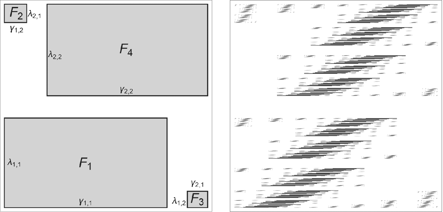
One can check numerically that a small neighborhood of the parameters $\gamma _{1,1}=\gamma _{2,2}=0.8$ , $\gamma _{1,2}=\gamma _{2,1}=0.1$ , $\unicode{x3bb} _{1,1}=\unicode{x3bb} _{2,2}=0.45$ and $\unicode{x3bb} _{2,1}=\unicode{x3bb} _{1,2}=0.09$ satisfies all three assumptions (2.2), (2.3) and (2.4). For a visual representation of the generalized 4-corner set, see Figure 1.

Figure 1

The first-level cylinders (left) and the attractor (right) of the generalized 4-corner set in Example 2.4.

Figure 1 Long description

The diagram consists of two square panels side-by-side.

Left Panel: Geometric construction of first-level cylinders. Four gray rectangles of varying sizes are positioned within a white square frame.

- Bottom-left: A large horizontal rectangle labeled F sub 1. Its left edge is lambda sub 1,1 and its bottom edge is gamma sub 1,1.

- Top-left: A small square labeled F sub 2. Its right edge is lambda sub 2,1 and its bottom edge is gamma sub 1,2.

- Top-right: A large horizontal rectangle labeled F sub 4. Its left edge is lambda sub 2,2 and its bottom edge is gamma sub 2,2.

- Bottom-right: A small square labeled F sub 3. Its left edge is lambda sub 1,2 and its top edge is gamma sub 2,1.

Right Panel: The resulting attractor. A complex, self-similar fractal pattern composed of numerous horizontal black and gray streaks. The density of the streaks mirrors the spatial arrangement of the four rectangles from the first panel, with two distinct horizontal bands of high-density clusters separated by a white gap, each containing further sub-structures of varying intensity.

2.4 Outline of the argument

Here, we provide an outline of the arguments of our main results, Theorems 1.3 and 1.4. The self-similar IFS $\mathcal {S}_{\underline {\unicode{x3bb} },\underline {t}}$ we consider has many exact overlaps at each level because many maps share the same fixed point. This implies our IFS does not satisfy the ESC. Thus, we cannot apply Theorem 1.2 by Hochman [Reference Hochman13] directly. However, the weaker version, the weak exponential separation condition (WESC; see Definition 3.4) allows exact overlaps, and by a direct consequence of Hochman’s seminal work [Reference Hochman13], Breuillard and Varjú [Reference Breuillard and Varjú6] determined the Hausdorff dimension of the self-similar measures in terms of random walk entropy under the WESC. However, they provided the proof only for the case of homogeneous similarity ratios. In §3, following the arguments of Breuillard and Varjú [Reference Breuillard and Varjú6], we provide a proof for Hausdorff dimension of the general self-similar measure under the WESC (see Theorem 3.5). This result is one of the main ingredients for proving our main result Theorem 1.3. In §4, we define a stronger version of WESC, namely the ESC for common fixed-point systems (CFS; see Definition 4.3), which is compatible with our self-similar IFS $\mathcal {S}_{\underline {\unicode{x3bb} },\underline {t}}$ . In that section, we prove the self-similar IFS $\mathcal {S}_{\underline {\unicode{x3bb} },\underline {t}}$ satisfies the ESC for CFS for typical parameters. One key fact is that the ESC for CFS provides a complete description of the exactly overlapping cylinders in the symbolic space. This is a significant advantage for computing the random walk entropy, which is otherwise a highly challenging task. In §5, we compute the value of the random walk entropy for the self-similar IFS $\mathcal {S}_{\underline {\unicode{x3bb} },\underline {t}}$ under the ESC for CFS. Now, by combining the results of §§4 and 5, we get Theorem 1.3. In §6, we prove another of our main theorems, Theorem 1.4. To prove that, we define the associated graph-directed self-similar IFS corresponding to our IFS $\mathcal {S}_{\underline {\unicode{x3bb} },\underline {t}}$ . We show that if IFS $\mathcal {S}_{\underline {\unicode{x3bb} },\underline {t}}$ satisfies the ESC for CFS, then the associated graph-directed self-similar IFS satisfies the graph-directed version of the ESC. We also prove that, under the ESC, the Hausdorff dimension of the attractor of the associated graph-directed self-similar IFS is determined by the unique exponent for which the spectral radius of the corresponding connection matrix is equal to $1$ . This result provides the required lower bound for Theorem 1.4, which coincides with the general upper bound.

3.1 Symbolic space

Let $\Sigma :=\{1,2,\ldots ,N\}^{\mathbb {N}}$ be the set of all infinite sequences with symbols from $\{1,2,\ldots ,N\}$ . The set $\Sigma $ is the symbolic space corresponding to the IFS $\mathcal {I}=\{f_1,\ldots ,f_N\}$ . Let $\mathbf {i}=i_{1}i_{2}\cdots \in \Sigma $ . We define $\mathbf {i}_{|_m}:=i_{1}i_{2}\cdots i_{m}$ for all $m\in \mathbb {N}$ . We denote the set of all finite sequences of length n with symbols from $\{1,2,\ldots , N\}$ by $\Sigma _{n}$ . Set $\Sigma ^{*}:=\bigcup _{n=1}^\infty \Sigma _{n}.$ The notation $|\mathbf {i}|$ denotes the length of the finite sequence $\mathbf {i}\in \Sigma ^*$ . For a symbol $i\in \{1,\ldots ,N\}$ and a finite word $\mathbf {i}\in \Sigma ^*$ , let $\#_i\mathbf {i}$ be the number of the appearances of the symbol i in the word $\mathbf {i}$ .

If $\mathbf {i}=i_1 i_2 \cdots i_n\in \Sigma ^{*}$ and $\mathbf {j}=j_1 j_2\cdots \in \Sigma ^{*} \cup \Sigma $ , then let $\mathbf {i}*\mathbf {j}=i_1 i_2 \cdots i_n j_1 j_2\cdots $ be the concatenation of $\mathbf {i}$ and $\mathbf {j}.$ The symbolic space $\Sigma $ equipped with the metric $\rho $ is a compact metric space, where the metric $\rho $ is defined as

$$ \begin{align*}\rho(\mathbf{i},\mathbf{j})=2^{-|\mathbf{i}\wedge\mathbf{j}|}\end{align*} $$

for $\mathbf {i},\mathbf {j}\in \Sigma $ , where $\mathbf {i}\wedge \mathbf {j}$ denotes the initial largest common segment of $\mathbf {i}$ and $\mathbf {j}$ . For $\mathbf {i}=i_1 i_2 \cdots i_n\in \Sigma ^{*},$ let $f_{\mathbf {i}}=f_{i_1}\circ f_{i_2}\circ \cdots \circ f_{i_n}$ and $r_{\mathbf {i}}=r_{i_1} r_{i_2}\cdots r_{i_n}.$ The mapping $\Pi : \Sigma \to A$ , defined by

$$ \begin{align*}\Pi(\mathbf{i})=\lim_{n\to\infty}f_{i_1}\circ f_{i_2}\circ \cdots \circ f_{i_n}(0)=\lim_{n\to \infty}f_{\mathbf{i}_{|_n}}(0),\end{align*} $$

is called the natural projection corresponding to the IFS $\mathcal {I}.$ For $\mathbf {i}=i_1 i_2 \cdots i_n\in \Sigma ^{*},$ set $\Pi (\mathbf {i}):=f_{i_1}\circ f_{i_2}\circ \cdots \circ f_{i_n}(0).$

3.2 Random walk entropy

In this section, we provide a more detailed description of the method by Hochman [Reference Hochman13].

Definition 3.1. Let $(X,\mathcal {B},\nu )$ be a probability space and $\xi =\{C_1,C_2,\ldots ,C_m\}$ be a measurable partition, that is, $\bigcup _{i=1}^mC_{i}=X,$ $C_i\in \mathcal {B}$ and $C_{i}\cap C_{j}=\emptyset $ for all ${i\ne j\in \{1,2,\ldots ,m\}}$ . Then the Shannon entropy H of the measure $\nu $ with respect to the partition $\xi $ is defined as follows

$$ \begin{align*}H(\nu,\xi)=-\sum_{i=1}^{m}\nu(C_{i})\log(\nu(C_{i})).\end{align*} $$

The self-similar IFS $\mathcal {I}$ with the probability vector $\mathbf {p}$ is known as a probabilistic self-similar IFS. We denote the probabilistic self-similar IFS by $(\mathcal {I},\mathbf {p}).$

Definition 3.2. The random walk entropy of the self-similar measure $\mu $ corresponding to the probabilistic self-similar IFS $(\mathcal {I},\mathbf {p})$ is defined as

$$ \begin{align*}h_{\mathrm{RW}}(\mu):=\lim_{n\to\infty}\frac{H_{n}}{n},\end{align*} $$

where $H_{n}$ is the Shannon entropy of the measure $\sum _{\mathbf {i}\in \Sigma _{n}}p_{\mathbf {i}}{\delta }_{f_{\mathbf {i}}},$ which is as follows:

$$ \begin{align*}H_{n}=-\sum_{\mathbf{i}\in \Sigma_{n}}p_{\mathbf{i}}\log\bigg(\sum_{\substack{\mathbf{j}\in \Sigma_{n}\\ f_{\mathbf{i}}\equiv f_{\mathbf{j}}}}p_{\mathbf{j}}\bigg).\end{align*} $$

The random walk entropy provides a more sophisticated upper bound on the dimension of the self-similar measures if exact overlaps occur. In particular, for every self-similar measure $\mu $ corresponding to the probabilistic self-similar IFS $(\mathcal {I},\mathbf {p})$ ,

$$ \begin{align*}\dim_{\mathrm{H}}(\mu)\leq \min\bigg\{1,\frac{h_{\mathrm{RW}}(\mu)}{\chi(\mathbf{p})}\bigg\};\end{align*} $$

see [Reference Bárány, Simon and Solomyak4, Theorem 3.2.7].

We now consider some of the following notation from Hochman’s work [Reference Hochman13]. For $n\in \mathbb {N}$ , $\mathcal {D}_{n}$ denote the partition of $\mathbb {R}$ into intervals of length $2^{-n}$ , that is,

$$ \begin{align*}\mathcal{D}_{n}=\bigg\{\bigg[\frac{k}{2^n},\frac{k+1}{2^n}\bigg): k\in \mathbb{Z}\bigg\}.\end{align*} $$

The notation $H(\nu , \mathcal {D}_n)$ denotes the Shannon entropy of the probability measure $\nu $ on $\mathbb {R}$ with respect to the partition $\mathcal {D}_n$ . For $m<n$ , $H(\nu , \mathcal {D}_n|\mathcal {D}_m)$ denotes the conditional entropy and is defined as $H(\nu , \mathcal {D}_n|\mathcal {D}_m):= H(\nu , \mathcal {D}_n)-H(\nu ,\mathcal {D}_m).$

The probability measure $\tilde {\nu }^{(n)}$ on $\mathbb {R}\times \mathbb {R}$ is defined by

$$ \begin{align*}\tilde{\nu}^{(n)}=\sum_{\mathbf{i}\in I^n}p_{\mathbf{i}}\delta_{(f_{\mathbf{i}}(0),r_{\mathbf{i}})},\end{align*} $$

where $\delta _x$ denotes the Dirac measure on the point x. We write $\tilde {\mathcal {D}}_n=\mathcal {D}_n\times \mathcal {F}$ for a partition on $\mathbb {R}\times \mathbb {R}$ , where $\mathcal {F}$ is the partition of $\mathbb {R}$ into points.

Theorem 3.3. [Reference Hochman13]

Let $\mu $ be the self-similar measure, and the probability measure $\tilde {\nu }^{(n)}$ be defined as above. If $\dim _{\mathrm {H}}(\mu )<1$ , then

$$ \begin{align*}\lim_{n\to \infty}\frac{1}{n'}H(\tilde{\nu}^{(n)},\tilde{\mathcal{D}}_{qn'}|\tilde{\mathcal{D}}_{n'})=0\quad \text{for all}\ q>1,\end{align*} $$

where $n'=\lfloor n \log ({1}/{r})\rfloor $ and $r= \prod _{i=1}^{N}{r_{i}}^{p_i}.$

Definition 3.4. We say that IFS $\mathcal {I}$ satisfies the WESC if there exists a sequence $\{n_{k}\}$ and there exists $b>1$ such that $n_{k}\to \infty $ and, for all $\mathbf {i},\mathbf {j}\in \Sigma _{n_k}$ , we have

$$ \begin{align*}\text{either } r_{\mathbf{i}}\ne r_{\mathbf{j}}\end{align*} $$

$$ \begin{align*} \quad\text{or } r_{\mathbf{i}}=r_{\mathbf{j}}\ \mathrm{and}\ f_{\mathbf{i}}(0)=f_{\mathbf{j}}(0)\iff f_{\mathbf{i}}\equiv f_{\mathbf{j}} \end{align*} $$

$$ \begin{align*}\text{or } r_{\mathbf{i}}=r_{\mathbf{j}}\ \mathrm{and}\ |f_{\mathbf{i}}(0)-f_{\mathbf{j}}(0)|>2^{-n_{k}' b}.\end{align*} $$

The following result is a direct consequence of Theorem 3.3, although it was not stated explicitly in Hochman’s seminal paper [Reference Hochman13]. It was observed by Breuillard and Varjú [Reference Breuillard and Varjú6], and they provided a proof for the case of homogeneous contraction ratios. We provide here the proof in the general case for completeness following Breuillard and Varjú [Reference Breuillard and Varjú6].

Theorem 3.5. Let $\mu $ be a self-similar measure corresponding to the probabilistic self-similar IFS $(\mathcal {I},\mathbf {p})$ . If IFS $\mathcal {I}$ satisfies the WESC, then

$$ \begin{align*}\dim_{\mathrm{H}}(\mu)=\min\bigg\{1,\frac{h_{\mathrm{RW}}(\mu)}{\chi(\mathbf{p})}\bigg\},\end{align*} $$

where $h_{\mathrm {RW}}(\mu )$ is the random walk entropy for the self-similar measure $\mu $ .

Proof. Since $\dim _{\mathrm {H}}(\mu )\leq ({h_{\mathrm {RW}}(\mu )}/{\chi (\mathbf {p})})$ , we may assume that $\dim _{\mathrm {H}}(\mu )<1.$ By Theorem 3.3, we have

$$ \begin{align*}\lim_{n\to \infty}\frac{1}{n'}H(\tilde{\nu}^{(n)},\tilde{\mathcal{D}}_{qn'}|\tilde{\mathcal{D}}_{n'})=0\quad \text{for all}\ q>1,\end{align*} $$

where $n'=\lfloor n \log ({1}/{r})\rfloor $ and $r= \prod _{i=1}^{N}{r_{i}}^{p_i}$ . Similarly to Hochman [Reference Hochman13], since $\mu $ is exact-dimensional, we get that

$$ \begin{align*}\lim_{n\to \infty}\frac{1}{n'}H(\tilde{\nu}^{(n)},\tilde{\mathcal{D}}_{n'})=\dim_{\mathrm{H}}(\mu).\end{align*} $$

Thus, for proving our result, it remains only to show that

(3.1) $$ \begin{align} \lim_{n\to \infty}\frac{1}{n'}H(\tilde{\nu}^{(n)},\tilde{\mathcal{D}}_{qn'})\geq \frac{h_{\mathrm{RW}}(\mu)}{\chi(\mathbf{p})} \end{align} $$

for some $q>1.$

We now prove expression (3.1). Let $q=b$ from Definition 3.4. For each $a\in \mathbb {R}$ , we have

$$ \begin{align*}\tilde{\nu}^{(n)}\bigg(\bigg[\frac{k}{2^{bn'}},\frac{k+1}{2^{bn'}}\bigg)\times \{a\}\bigg)=\sum_{\substack{{\mathbf{j}}\in \Sigma_{n}\\ r_{\mathbf{j}}=a}}p_{\mathbf{j}}\delta_{f_{\mathbf{j}}(0)}\bigg[\frac{k}{2^{bn'}},\frac{k+1}{2^{bn'}}\bigg).\end{align*} $$

Thus, the Shannon entropy of the probability measure $\tilde {\nu }^{(n_k)}$ on $\mathbb {R}\times \mathbb {R} $ with respect to the partition $\tilde {\mathcal {D}}_{bn_{k}'}$ is

$$ \begin{align*}& H(\tilde{\nu}^{(n_k)},\tilde{\mathcal{D}}_{bn_{k}'})\\ &\quad =-\sum_{\substack{a\in \mathbb{R}\\ \text{ there exists }~ r_{\mathbf{i}}=a}}\sum_{l\in \mathbb{Z}} \tilde{\nu}^{(n_k)}\bigg(\bigg[\frac{l}{2^{bn_{k}'}},\frac{l+1}{2^{bn_{k}'}}\!\bigg)\times \{a\}\!\bigg) \log\bigg(\!\tilde{\nu}^{(n_k)}\bigg(\bigg[\frac{l}{2^{bn_{k}'}},\frac{l+1}{2^{bn_{k}'}}\!\bigg)\times \{a\}\!\bigg)\!\bigg)\\&\quad =-\sum_{\substack{a\in \mathbb{R}\\ \text{ there exists }~ r_{\mathbf{i}}=a}}\sum_{l\in \mathbb{Z}}\!\bigg(\!\sum_{\substack{{\mathbf{j}}\in \Sigma_{n_{k}}\\ r_{\mathbf{j}}=a}}p_{\mathbf{j}}\delta_{f_{\mathbf{j}}(0)}\bigg[\frac{l}{2^{bn_{k}'}},\frac{l+1}{2^{bn_{k}'}}\!\bigg)\!\bigg) \log\!\bigg(\!\sum_{\substack{{\mathbf{j}}\in \Sigma_{n_{k}}\\ r_{\mathbf{j}}= a}}\!\! p_{\mathbf{j}}\delta_{f_{\mathbf{j}}(0)}\bigg[\frac{l}{2^{bn_{k}'}},\frac{l+1}{2^{bn_{k}'}}\!\bigg)\!\hspace{-0.5pt}\bigg). \end{align*} $$

Since the IFS $\mathcal {I}$ satisfies the WESC, we have

$$ \begin{align*} H(\tilde{\nu}^{(n_k)},\tilde{\mathcal{D}}_{bn_{k}'})&=-\sum_{\substack{a\in \mathbb{R}\\ \text{ there exists }~ r_{\mathbf{i}}=a}}\bigg(\sum_{\substack{{\mathbf{j}}\in \Sigma_{n_k}\\ f_{\mathbf{i}}\equiv f_{\mathbf{j}}}}p_{\mathbf{j}}\bigg)\log\bigg(\sum_{\substack{{\mathbf{j}}\in \Sigma_{n_{k}}\\ f_{\mathbf{i}}\equiv f_{\mathbf{j}}}}p_{\mathbf{j}}\bigg)\\&= -\sum_{{\mathbf{i}}\in I^{n_{k}}}p_{\mathbf{i}} \log\bigg(\sum_{\substack{{\mathbf{j}}\in \Sigma_{n_k}\\ f_{\mathbf{i}}\equiv f_{\mathbf{j}}}}p_{\mathbf{j}}\bigg). \end{align*} $$

This implies that

$$ \begin{align*} \lim_{k\to \infty}\frac{1}{n_{k}'}H(\tilde{\nu}^{(n_k)},\tilde{\mathcal{D}}_{bn_{k}'})\geq \frac{h_{\mathrm{RW}}(\mu)}{\chi(\mathbf{p})}, \end{align*} $$

which completes the proof.

4.1 Technical lemmas

We begin by discussing some general results for later purposes, which will be particularly useful in describing the dimension theory of self-similar IFSs with a common fixed-point structure.

Let us consider a self-similar IFS $\mathcal {F}$ on $\mathbb {R}$ ,

(4.1) $$ \begin{align} \mathcal{F}:=\{f_{i}(x)=\unicode{x3bb}_{i}x\}_{i=1}^{M_1}\cup\{f_{i}(x)=\unicode{x3bb}_{i}x+c_i\}_{i=M_1+1}^{M_2}, \end{align} $$

where $M_2>M_1\geq 2$ . Suppose that there exist $\epsilon ,A>0$ such that:

1. (1) $\unicode{x3bb} _{i}\in [\epsilon ,1-\epsilon ]~\text { for all }i\in \{1,2,\ldots ,M_1\}$ and $|\unicode{x3bb} _{i}|\in [\epsilon ,1-\epsilon ]\text { for all }i\in \{M_{1}+1, M_{1}+2,\ldots ,M_2\}$ ;

2. (2) $f_{i}[0,A]\subseteq [\epsilon ,A] ~\text { for all }~i\in \{M_{1}+1,\ldots ,M_2\}$ .

Let $\Sigma =\{1,\ldots ,M_2\}^{\mathbb {N}}$ be the symbolic space and let $\Pi $ be the natural projection corresponding to the IFS $\mathcal {F}$ . Throughout the section, we assume that $A>\epsilon >0$ are arbitrary but fixed.

For an $\mathbf {i}\in \Sigma $ , we define the ‘first block’ $b_1^{\mathbf {i}}$ of $\mathbf {i}$ as follows: if $i_1\geq M_1+1$ then ${b_1^{\mathbf {i}}=i_1}$ . Otherwise, let $|b_1^{\mathbf {i}}|:=\min \{k\geq 1:i_k\geq M_1+1\}-1$ , and if $|b_1^{\mathbf {i}}|=\infty $ then let $b_1^{\mathbf {i}}=\mathbf {i}$ , otherwise let $b_1^{\mathbf {i}}:=\mathbf {i}_{|_{|b_1^{\mathbf {i}}|}}$ .

We say that for $\mathbf {i},\mathbf {j}\in \Sigma $ , the first blocks are disjoint if the sets formed by the symbols in the first blocks $b_1^{\mathbf {i}}$ and $b_1^{\mathbf {j}}$ are disjoint. We denote this by $b_{1}^{\mathbf {i}}\cap b_{1}^{\mathbf {j}}=\emptyset $ . In other words, $\min \{\#_ib_{1}^{\mathbf {i}},\#_ib_{1}^{\mathbf {j}}\}=0$ for every $1\leq i\leq M_2$ .

In the next two lemmas, we will follow and modify techniques of Kamalutdinov and Tetenov [Reference Kamalutdinov and Tetenov16].

We define a set as follows:

$$ \begin{align*} \tilde{\mathcal{A}}_{1} & =\bigg\{(\mathbf{i},\mathbf{j})\in \Sigma\times \Sigma: 1\leq i_1,j_1\leq M_1\ \mathrm{and}\ b_{1}^{\mathbf{i}}\cap b_{1}^{\mathbf{j}} =\emptyset \\& \,\qquad\mathrm{and}\ \frac{\unicode{x3bb}_{b_{1}^{\mathbf{i}}}}{\unicode{x3bb}_{b_{1}^{\mathbf{j}}}}\notin \bigg(\frac{\epsilon}{2A},\frac{2A}{\epsilon }\bigg)\ \mathrm{and}\ b_{1}^{\mathbf{i}}\ne \mathbf{i},b_{1}^{\mathbf{j}}\ne \mathbf{j}\bigg\}.\end{align*} $$

Lemma 4.1. Let $\mathcal {F}$ be the self-similar IFS of the form (4.1) with natural projection $\Pi $ . Let $A>\epsilon >0$ . Then, for every $\underline {\unicode{x3bb} }=(\unicode{x3bb} _i)_{i=1}^{M_2}$ satisfying (1)–(2) and for every pair $(\mathbf {i},\mathbf {j})\in \tilde {\mathcal {A}}_{1}$ ,

$$ \begin{align*}|\Pi(\mathbf{i})-\Pi(\mathbf{j})|\geq {\epsilon}^{3\max\{|b_{1}^{\mathbf{i}}|,|b_{1}^{\mathbf{j}}|\}}.\end{align*} $$

Proof. Without loss of generality, we assume that $({\unicode{x3bb} _{b_{1}^{\mathbf {i}}}}/{\unicode{x3bb} _{b_{1}^{\mathbf {j}}}})\geq ({2 A}/{\epsilon })$ ; the other case can be proven similarly. Since $b_{1}^{\mathbf {i}}\ne \mathbf {i},b_{1}^{\mathbf {j}}\ne \mathbf {j}$ and $f_{i}[0,A]\subseteq [\epsilon ,A]$ for all $i\in \{M_{1}+1,\ldots ,M_2\}$ , we have

$$ \begin{align*}\Pi(\mathbf{i})\in f_{b_{1}^{\mathbf{i}}}([\epsilon,A])\quad\text{and}\quad\Pi(\mathbf{j})\in f_{b_{1}^{\mathbf{j}}}([\epsilon,A]).\end{align*} $$

Thus, we get

$$ \begin{align*} \Pi(\mathbf{i})-\Pi(\mathbf{j})=\unicode{x3bb}_{b_{1}^{\mathbf{i}}}x- \unicode{x3bb}_{b_{1}^{\mathbf{j}}}y \end{align*} $$

for some $x,y\in [\epsilon ,A]$ . This implies that

$$ \begin{align*}\begin{aligned} \Pi(\mathbf{i})-\Pi(\mathbf{j})&\geq \unicode{x3bb}_{b_{1}^{\mathbf{i}}} \epsilon- \unicode{x3bb}_{b_{1}^{\mathbf{j}}}A=\unicode{x3bb}_{b_{1}^{\mathbf{i}}} \epsilon \bigg(1-\frac{\unicode{x3bb}_{b_{1}^{\mathbf{j}}} A}{\unicode{x3bb}_{b_{1}^{\mathbf{i}}} \epsilon}\bigg)\geq \frac{\epsilon}{2} \unicode{x3bb}_{b_{1}^{\mathbf{i}}}\geq {\epsilon}^{3|b_{1}^{\mathbf{i}}|}. \end{aligned}\\[-43pt]\end{align*} $$

Let $N_{0}=\lceil ({(1-\epsilon )(2A+\epsilon )})/{\epsilon ^3} \rceil +1.$ We define a set as follows:

$$ \begin{align*} \tilde{\mathcal{A}}_{2}&=\bigg\{(\mathbf{i},\mathbf{j})\in \Sigma\times \Sigma: 1\leq i_1,j_1\leq M_1\ \mathrm{and}\ b_{1}^{\mathbf{i}}\cap b_{1}^{\mathbf{j}} =\emptyset\\& \qquad \mathrm{and}\ \frac{\unicode{x3bb}_{b_{1}^{\mathbf{i}}}}{\unicode{x3bb}_{b_{1}^{\mathbf{j}}}}\in \bigg(\frac{\epsilon}{2A},\frac{2A}{\epsilon}\bigg)\ \mathrm{and}\ b_{1}^{\mathbf{i}}\ne \mathbf{i},b_{1}^{\mathbf{j}}\ne \mathbf{j}\\& \qquad \mathrm{and}\ \max_{1\leq k\leq M_1}\{\max\{\#_kb_{1}^{\mathbf{i}},\#_kb_{1}^{\mathbf{j}}\}\}>N_{0}\bigg\} \end{align*} $$

Lemma 4.2. Let $\mathcal {F}$ be the self-similar IFS of the form (4.1) with natural projection $\Pi $ . Let $A>\epsilon >0$ . Then there exists a constant $C>0$ such that for every $\underline {\unicode{x3bb} }=(\unicode{x3bb} _i)_{i=1}^{M_2}$ satisfying (1)–(2) and for every $(\mathbf {i},\mathbf {j})\in \tilde {\mathcal {A}}_{2}$ ,

$$ \begin{align*}\bigg{|}\frac{\partial(\Pi(\mathbf{i})-\Pi(\mathbf{j}))}{\partial \unicode{x3bb}_{k}}\bigg{|}\geq C{\epsilon}^{\max\{|b_{1}^{\mathbf{i}}|,|b_{1}^{\mathbf{j}}|\}},\end{align*} $$

where k is such that $\max \{\#_kb_{1}^{\mathbf {i}},\#_kb_{1}^{\mathbf {j}}\}>N_0$ .

Proof. Let $(\mathbf {i},\mathbf {j})\in \tilde {\mathcal {A}}_{2}$ . For simplicity, let $m_k=\#_kb_{1}^{\mathbf {i}}$ and $n_k{\kern-1pt}={\kern-1pt}\#_kb_{1}^{\mathbf {j}}$ for $k{\kern-1pt}\in{\kern-1pt} \{1,2,\ldots , M_1\}$ . Without loss of generality, we assume that $m_r>N_0$ for some $r\in \{1,2,\ldots , M_1\}$ . By definition, $n_r=0$ . Let $\unicode{x3bb} _{r}'\in [\epsilon , 1-\epsilon ]$ be such that $\unicode{x3bb} _r<\unicode{x3bb} _r'$ and

$$ \begin{align*}\frac{\epsilon}{2A} \leq \frac{(\unicode{x3bb}_r')^{m_r}\prod_{i=1,\ i\neq r}^{M_1}\unicode{x3bb}_{i}^{m_i}}{\prod_{i=1}^{M_1}\unicode{x3bb}_{i}^{n_i}}\leq \frac{2A}{\epsilon}.\end{align*} $$

Let $\delta =\unicode{x3bb} _{r}'-\unicode{x3bb} _{r}>0$ . Then, by using the mean value theorem, we have

$$ \begin{align*}m_r \unicode{x3bb}_{r}^{m_{r}-1}\leq\frac{(\unicode{x3bb}_{r}')^{m_r}-\unicode{x3bb}_{r}^{m_r}}{\unicode{x3bb}_{r}'-\unicode{x3bb}_{r}}=\frac{|(\unicode{x3bb}_{r}')^{m_r}-\unicode{x3bb}_{r}^{m_r}|}{\delta}\leq m_r (\unicode{x3bb}_{r}')^{m_{r}-1}.\end{align*} $$

Now we define another self-similar IFS,

$$ \begin{align*}\mathcal{F}'=\{\mathcal{F}\setminus\{f_{r}(x)=\unicode{x3bb}_{r} x\}\}\cup\{f'_{r}(x)=\unicode{x3bb}_{r}' x\}.\end{align*} $$

This is simply obtained from the IFS $\mathcal {F}$ by replacing the map $f_{r}$ by $f_{r}'$ . Let $\Pi '$ be the natural projection corresponding to the IFS $\mathcal {F}'$ . Thus, by the displacement lemma by Kamalutdinov and Tetenov [Reference Kamalutdinov and Tetenov16, Theorem 17], we have

(4.2) $$ \begin{align} |\Pi(\mathbf{i})-\Pi'(\mathbf{i})|\leq \frac{\delta}{\epsilon}\quad \text{for all}\ \mathbf{i}\in \Sigma. \end{align} $$

For the given pair $(\mathbf {i},\mathbf {j})\in \Sigma \times \Sigma $ , we have

$$ \begin{align*}\Pi(\mathbf{i})=f_{1}^{m_1}\circ \cdots \circ f_{M_1}^{m_{M_1}}(f_{\tilde{i}}(\Pi(\hat{\mathbf{i}}))), \Pi(\mathbf{j})=f_{1}^{n_1}\circ \cdots\circ f_{M_1}^{n_{M_1}}(f_{\tilde{j}}(\Pi(\hat{\mathbf{j}}))),\end{align*} $$

$$ \begin{align*}\Pi^{\prime}(\mathbf{i})=f_{1}^{m_1}\circ \cdots \circ f_{r-1}^{m_{r-1}}\circ {f}_{{r}}^{{\prime}m_{r}}\circ f_{{r+1}}^{m_{r+1}}\circ \cdots \circ f_{M_1}^{m_{M_1}}(f_{\tilde{i}}(\Pi^{\prime}(\hat{\mathbf{i}}))), \end{align*} $$

$$ \begin{align*}\Pi^{\prime}(\mathbf{j})=f_{1}^{n_1}\circ\cdots\circ f_{M_1}^{n_l}(f_{\tilde{j}}(\Pi^{\prime}(\hat{\mathbf{j}}))),\end{align*} $$

for some $\tilde {i},\tilde {j}\in \{M_{1}+1,\ldots ,M_2\}$ and $\hat {\mathbf {i}},\hat {\mathbf {j}}\in \Sigma .$ We now estimate the expression $|(\Pi (\mathbf {i})-\Pi (\mathbf {j}))-(\Pi '(\mathbf {i})-\Pi '(\mathbf {j}))|$ . We have

$$ \begin{align*} &|(\Pi(\mathbf{i})-\Pi(\mathbf{j}))-(\Pi^{\prime}(\mathbf{i})-\Pi^{\prime}(\mathbf{j}))|\\[4pt]&\quad=|\Pi(\mathbf{i})-\Pi^{\prime}(\mathbf{i})+\Pi^{\prime}(\mathbf{j})-\Pi(\mathbf{j})|\\[4pt]&\quad\geq |f_{1}^{m_1}\circ \cdots \circ f_{M_1}^{m_{M_1}}(f_{\tilde{i}}(\Pi(\hat{\mathbf{i}})))\\[4pt]&\quad\quad -f_{1}^{m_1}\circ \cdots \circ f_{r-1}^{m_{r-1}}\circ {f}_{{r}}^{{\prime}m_{r}}\circ f_{{r+1}}^{m_{r+1}}\circ \cdots \circ f_{M_1}^{m_{M_1}}(f_{\tilde{i}}(\Pi^{\prime}(\hat{\mathbf{i}})))|\\[4pt]&\quad\quad -|\Pi'(\mathbf{j})-\Pi(\mathbf{j})|\\[4pt]&\quad\geq|f_{1}^{m_1}\circ \cdots \circ f_{M_1}^{m_{M_1}}(f_{\tilde{i}}(\Pi^{\prime}(\hat{\mathbf{i}})))\\[4pt]&\quad\quad -f_{1}^{m_1}\circ \cdots \circ f_{r-1}^{m_{r-1}}\circ {f}_{{r}}^{{\prime}m_{r}}\circ f_{{r+1}}^{m_{r+1}}\circ \cdots \circ f_{M_1}^{m_{M_1}}(f_{\tilde{i}}(\Pi^{\prime}(\hat{\mathbf{i}})))|\\[4pt]&\quad\quad-|f_{1}^{m_1}\circ \cdots \circ f_{M_1}^{m_{M_1}}(f_{\tilde{i}}(\Pi(\hat{\mathbf{i}})))-f_{1}^{m_1}\circ \cdots \circ f_{M_1}^{m_{M_1}}(f_{\tilde{i}}(\Pi^{\prime}(\hat{\mathbf{i}})))|\\[4pt]&\quad\quad -|\Pi^{\prime}(\mathbf{j})-\Pi(\mathbf{j})|\\[4pt]&\quad=:L_1-L_2-L_3. \end{align*} $$

To estimate the above expression, we need to individually estimate the values of $L_1$ , $L_2$ , and $L_3$ . Thus, we have

$$ \begin{align*} L_1&=|f_{1}^{m_1}\circ \cdots \circ f_{M_1}^{m_{M_1}}(f_{\tilde{i}}(\Pi^{\prime}(\hat{\mathbf{i}})))\\[4pt]&\quad -f_{1}^{m_1}\circ \cdots \circ f_{r-1}^{m_{r-1}}\circ {f}_{{r}}^{{\prime}m_{r}}\circ f_{{r+1}}^{m_{r+1}}\circ \cdots \circ f_{M_1}^{m_{M_1}}(f_{\tilde{i}}(\Pi^{\prime}(\hat{\mathbf{i}})))|\\[4pt]&=|{\unicode{x3bb}_{r}^{\prime}}^{m_{r}}-\unicode{x3bb}_{r}^{m_{r}}|\prod_{\substack{i=1\\ i\neq r}}^{M_1}\unicode{x3bb}_{i}^{m_i}|f_{\tilde{i}}(\Pi^{\prime}(\hat{\mathbf{i}}))|\geq m_r\unicode{x3bb}_r^{-1}\delta\prod_{i=1}^{M_1}\unicode{x3bb}_{i}^{m_i}\epsilon\geq \frac{N_0\delta \epsilon}{1-\epsilon} \unicode{x3bb}_{b_{1}^{\mathbf{i}}}. \end{align*} $$

On the other hand,

$$ \begin{align*} L_2&=|f_{1}^{m_1}\circ \cdots \circ f_{M_1}^{m_{M_1}}(f_{\tilde{i}}(\Pi(\hat{\mathbf{i}})))-f_{1}^{m_1}\circ \cdots \circ f_{M_1}^{m_{M_1}}(f_{\tilde{i}}(\Pi^{\prime}(\hat{\mathbf{i}})))|\\&\leq \unicode{x3bb}_{b_{1}^{\mathbf{i}}}|\Pi(\hat{\mathbf{i}})-\Pi^{\prime}(\hat{\mathbf{i}})|\leq \frac{\delta}{\epsilon} \unicode{x3bb}_{b_{1}^{\mathbf{i}}}, \end{align*} $$

where we used (4.2). Moreover,

$$ \begin{align*} L_3&=|\Pi^{\prime}(\mathbf{j})-\Pi(\mathbf{j})|=|f_{1}^{n_1}\circ\cdots\circ f_{M_1}^{n_{M_1}}(f_{\tilde{j}}(\Pi(\hat{\mathbf{j}})))-f_{1}^{n_1}\circ\cdots\circ f_{M_1}^{n_{M_1}}(f_{\tilde{j}}(\Pi^{\prime}(\hat{\mathbf{j}})))|\\ &=\unicode{x3bb}_{b_{1}^{\mathbf{j}}}|\unicode{x3bb}_{\tilde{j}}||\Pi(\hat{\mathbf{j}})-\Pi^{\prime}(\hat{\mathbf{j}})|\leq \unicode{x3bb}_{b_{1}^{\mathbf{j}}}(1-\epsilon)\frac{\delta}{\epsilon}, \end{align*} $$

where we used the estimate (4.2) again. Thus, we get

$$ \begin{align*} L_1-L_2\geq \bigg(\frac{N_{0}\epsilon}{1-\epsilon}-\frac{1}{\epsilon}\bigg)\unicode{x3bb}_{b_{1}^{\mathbf{i}}}\delta\geq \frac{\epsilon\delta}{2A}\bigg(\frac{N_{0}\epsilon}{1-\epsilon}-\frac{1}{\epsilon}\bigg) \unicode{x3bb}_{b_{1}^{\mathbf{j}}}. \end{align*} $$

Thus, by using the above estimates, we get

$$ \begin{align*} L_{1}-L_{2}-L_{3}\geq \bigg(\frac{N_{0}\epsilon^{3}-(1-\epsilon)(2A+\epsilon)}{2A(1-\epsilon)\epsilon}\bigg)\unicode{x3bb}_{b_{1}^{\mathbf{j}}} \delta\geq \delta\bigg(\frac{N_{0}\epsilon^{3}-(1-\epsilon)(2A+\epsilon)}{2A(1-\epsilon)\epsilon}\bigg)\epsilon^{|b_{1}^{\mathbf{j}}|}. \end{align*} $$

Choosing $C=(({N_{0}\epsilon ^{3}-(1-\epsilon )(2A+\epsilon )})/{2A(1-\epsilon )\epsilon }),$ and since $N_{0}{\kern-1pt}={\kern-1pt}\lceil ((1{\kern-1pt}-{\kern-1pt}\epsilon ) (2A+\epsilon )) /{{\epsilon }^3} \rceil +1,$ we have $C>0.$ This implies that

$$ \begin{align*}|(\Pi(\mathbf{i})-\Pi(\mathbf{j}))-(\Pi^{\prime}(\mathbf{i})-\Pi^{\prime}(\mathbf{j}))|\geq C{\epsilon}^{|b_{1}^{\mathbf{j}}|}\delta.\end{align*} $$

This also implies that

$$ \begin{align*}\bigg{|}\frac{\partial(\Pi(\mathbf{i})-\Pi(\mathbf{j}))}{\partial{\unicode{x3bb}_{r}}}\bigg{|}\geq C{\epsilon}^{|b_{1}^{\mathbf{j}}|}\geq C{\epsilon}^{\max\{|b_{1}^{\mathbf{i}}|,|b_{1}^{\mathbf{j}}|\}}.\end{align*} $$

This completes the proof.

4.2 Block structure

We now give a more detailed description of the coding of IFS $\mathcal {S}$ with common fixed-point structure defined in (1.3). Let us recall the definition. Let $N\geq 2$ be an integer, and for every $1\leq i\leq N$ , let $n_i\geq 1$ be an integer. Let

(4.3) $$ \begin{align} \mathcal{S}=\{f_{i,j}=\unicode{x3bb}_{i,j}x+t_{i}(1-\unicode{x3bb}_{i,j}): 1\leq i\leq N\ \mathrm{and}\ 1\leq j\leq n_i\}, \end{align} $$

where $\unicode{x3bb} _{i,j}\in (0,1)$ and $t_i\in \mathbb {R}$ . Without loss of generality, we assume that $0< t_1 < t_2 <\cdots < t_N.$

Let $I=\{(i,j):1\leq i\leq N,\ 1\leq j\leq n_i\}$ and let $\Sigma =I^{\mathbb {N}}$ be the symbolic space corresponding to IFS $\mathcal {S}$ . Denote by $\Sigma _n$ the set n-length finite sequences formed by the symbols of I, and let $\Sigma ^*=\bigcup _{n=0}^\infty \Sigma _n$ . Denote the length of $\mathbf {i}\in \Sigma ^*$ by $|\mathbf {i}|$ . We will use the convention that $|\mathbf {i}|=\infty $ for $\mathbf {i}\in \Sigma $ . Denote by $\sigma \colon \Sigma \to \Sigma $ the usual left-shift operator. We extend $\sigma $ to $\Sigma ^*$ by $\sigma (i_1,\ldots ,i_n)=(i_2,\ldots ,i_n)$ .

For each $\mathbf {i}\in \Sigma \cup \Sigma ^*$ , we define the following unique block representation. For ${\mathbf {i}=((i_1,j_1),(i_2,j_2),\ldots )}$ , let $|b_1^{\mathbf {i}}|:=\max \{k\geq 1:i_1=i_\ell \text { for all }1\leq \ell \leq k\}$ . If $|b_1^{\mathbf {i}}|=|\mathbf {i}|$ then let $b_1^{\mathbf {i}}:=\mathbf {i}$ , otherwise let $b_1^{\mathbf {i}}:=\mathbf {i}_{|_{|b_1^{\mathbf {i}}|}}$ . Then we define by induction. Suppose that $b_1^{\mathbf {i}},\ldots ,b_n^{\mathbf {i}}$ are defined and finite. Then let

$$ \begin{align*} |b_{n+1}^{\mathbf{i}}|:=\max\{k\geq1:i_{|b_1^{\mathbf{i}}|+\cdots+|b_n^{\mathbf{i}}|+1}=i_{|b_1^{\mathbf{i}}|+\cdots+|b_n^{\mathbf{i}}|+\ell}\text{ for all }1\leq\ell\leq k\}. \end{align*} $$

If $|b_{n+1}^{\mathbf {i}}|=|\sigma ^{|b_1^{\mathbf {i}}|+\cdots +|b_n^{\mathbf {i}}|}\mathbf {i}|$ then let $b_{n+1}^{\mathbf {i}}:=\sigma ^{|b_1^{\mathbf {i}}|+\cdots +|b_n^{\mathbf {i}}|}\mathbf {i}$ , and so $\mathbf {i}=b_1^{\mathbf {i}}\cdots b_n^{\mathbf {i}}b_{n+1}^{\mathbf {i}}$ . Otherwise, let $b_{n+1}^{\mathbf {i}}:=(\sigma ^{|b_1^{\mathbf {i}}|+\cdots +|b_n^{\mathbf {i}}|}\mathbf {i})_{|_{|b_{n+1}^{\mathbf {i}}|}}$ . Let $B^{\mathbf {i}}$ denote the number of block in $\mathbf {i}$ . For $\mathbf {i}\in \Sigma $ , the maps in each block $b_{l}^{\mathbf {i}}$ correspond to the same fixed points. The maps having the same fixed point are commutative. We write $t_{b_l^{\mathbf {i}}}$ for the common fixed point of the maps in the block $b_{l}^{\mathbf {i}}$ , which is also the fixed point of the map $f_{b_l^{\mathbf {i}}}$ . Thus, any $\mathbf {i}\in \Sigma $ can be written uniquely as countably (but possibly finitely) many finite sequences:

(4.4) $$ \begin{align} \mathbf{i}=\underbrace{(i_1,j_1)\cdots (i_1,j_l)}_{b_{1}^{\mathbf{i}}}\underbrace{(i_{l+1},j_{l+1})\cdots (i_{l+1},j_m)}_{b_{2}^{\mathbf{i}}} (i_{m+1},j_{m+1})\cdots. \end{align} $$

Note that the maps corresponding to the symbols from the same block share the same fixed point.

Let $\Pi : \Sigma \to [t_1,t_N]$ be the natural projection corresponding to the IFS $\mathcal {S}.$ Simple algebraic manipulations show that for every $\mathbf {i}\in \Sigma $ with $B^{\mathbf {i}}=\infty $ ,

$$ \begin{align*} \Pi(\mathbf{i})=t_{b_{1}^{\mathbf{i}}}+\sum_{l=1}^{\infty}\unicode{x3bb}_{b_{1}^{\mathbf{i}}}\unicode{x3bb}_{b_{2}^{\mathbf{i}}}\cdots \unicode{x3bb}_{b_{l}^{\mathbf{i}}}(t_{b_{l+1}^{\mathbf{i}}}-t_{b_{l}^{\mathbf{i}}}), \end{align*} $$

where $\unicode{x3bb} _{b_{l}^{\mathbf {i}}}$ represents the similarity ratio of the map corresponding to the lth block in the infinite sequence $\mathbf {i}$ . For a finite $\mathbf {i}\in \Sigma ^*$ , we will write $\Pi (\mathbf {i})=f_{\mathbf {i}}(0)$ with a slight abuse of notation. Observe that $\Pi $ is an analytic map of $\underline {\unicode{x3bb} }=(\unicode{x3bb} _{i,j})_{(i,j)\in I}$ and a linear map of ${\underline {t}=(t_i)_{i=1}^N}$ for every $\mathbf {i}\in \Sigma \cup \Sigma ^*$ . In particular, $\Pi $ is analytic over ${\underline {\unicode{x3bb} }\in (-1+\epsilon ,1-\epsilon )^{\sum _{i=1}^Nn_i}}$ , which fact will be used for later purposes.

For a finite word $\mathbf {i}\in \Sigma ^*$ , let $\#_{i,j}\mathbf {i}$ denote the number of symbols $(i,j)$ appearing in $\mathbf {i}$ . For $\mathbf {i},\mathbf {j}\in \Sigma \cup \Sigma ^*$ , we say that $\mathbf {i},\mathbf {j}$ have the same block structure if $B^{\mathbf {i}}=B^{\mathbf {j}}$ and for every $1\leq l\leq B^{\mathbf {i}}$ , $t_{b_l^{\mathbf {i}}}=t_{b_l^{\mathbf {j}}}$ and $\#_{i,j}b_l^{\mathbf {i}}=\#_{i,j}b_l^{\mathbf {j}}$ for every $(i,j)\in I$ . Note that if $\mathbf {i},\mathbf {j}\in \Sigma ^*$ have the same block structure then $f_{\mathbf {i}}\equiv f_{\mathbf {j}}$ .

We now define a special form of the WESC adapted to CFS.

Definition 4.3. We say that the IFS $\mathcal {S}$ satisfies the ESC for CFS if there exist $N\in \mathbb {N}$ and $b>1$ such that for every $n\geq N$ and every $\mathbf {i}, \mathbf {j}\in \Sigma _n$ with $\unicode{x3bb} _{\mathbf {i}}=\unicode{x3bb} _{\mathbf {j}}$ , we have the following property:

(4.5) $$ \begin{align} \text{either } \mathbf{i} , \mathbf{j} \text{ have the same block structure or } |\Pi({\mathbf{i}})-\Pi({\mathbf{j}})|>2^{-b n}. \end{align} $$

Let us note that one can relax the definition of the exponential separation for CFS through a subsequence of natural numbers n for which (4.5) holds. However, it would require a slight change in the proofs and the definition of the exceptional sets.

One can see that the ESC for CFS for the IFS $\mathcal {S}$ implies that the IFS $\mathcal {S}$ satisfies the WESC (see Definition 3.4). The ESC for CFS provides a complete description of the overlapping cylinders via symbolic space; see §5.

We say that the finite words $\mathbf {i},\mathbf {j}\in \Sigma ^*$ are disjoint if $\min \{\#_{i,j}\mathbf {i},\#_{i,j}\mathbf {j}\}=0$ for every $(i,j)\in I$ . We will denote this with a slight abuse of notation by $\mathbf {j}\cap \mathbf {i}=\emptyset $ .

4.3 Two-fixed-point system

Next, we discuss the ESC for CFS in the case of two-fixed-point systems. We consider the following IFS, having only two fixed points:

(4.6) $$ \begin{align} \mathcal{J}=\{f_{1,i}(x)=\unicode{x3bb}_{1,i} x\}_{i=1}^{n_1}\cup \{f_{2,i}(x)=\unicode{x3bb}_{2,i} x+(1-\unicode{x3bb}_{2,i})\}_{i=1}^{n_2}. \end{align} $$

Clearly, the IFS $\mathcal {J}$ is a special case of the family of IFSs defined in (4.3), where $t_1=0$ and $t_2=1$ . Let $\Sigma $ be the symbolic space corresponding to the IFS $\mathcal {J}$ with symbols $I=\{(i,j): i\in \{1,2\}, j\in \{1,\ldots ,n_i\}\}.$

Write $L=n_1+n_2$ , and denote by $\underline {\unicode{x3bb} }=(\unicode{x3bb} _{i,j})_{(i,j)\in I}\in (0,1)^{L}$ the vector of contraction ratios. Observe that for every $\epsilon>0$ such that $\epsilon \leq \min _{(i,j)\in I}\min \{\unicode{x3bb} _{i,j},1-\unicode{x3bb} _{i,j}\}$ we have $L_{\mathcal {J}}\subseteq [0,1-\epsilon ]$ and $R_{\mathcal {J}}\subseteq [\epsilon ,1]$ , where $L_{\mathcal {J}}:=\bigcup _{i=1}^{n_1}f_{1,i}([0,1])$ and $R_{\mathcal {J}}:=\bigcup _{i=1}^{n_2}f_{2,i}([0,1]).$

Let $\Pi $ be the natural projection corresponding to the IFS $\mathcal {J}$ . For $\mathbf {i},\mathbf {j}\in \Sigma $ , we define

$$ \begin{align*} \Delta_{\mathbf{i},\mathbf{j}}(\underline{\unicode{x3bb}})=\Pi(\mathbf{i})-\Pi(\mathbf{j}). \end{align*} $$

Let us define the following set of pairs:

(4.7) $$ \begin{align} \mathcal{B}:=\{(\mathbf{i},\mathbf{j})\in \Sigma\times \Sigma: b_1^{\mathbf{i}}\cap b_1^{\mathbf{j}}=\emptyset\ \mathrm{and}\ b_1^{\mathbf{i}}\neq\mathbf{i}\ \mathrm{and}\ b_1^{\mathbf{j}}\neq\mathbf{j}\}. \end{align} $$

We divide the set $\mathcal {B}$ further:

(4.8) $$ \begin{align} \mathcal{B}_{1}:=\{(\mathbf{i},\mathbf{j})\in \mathcal{B}: t_{b_{1}^{\mathbf{i}}}\ne t_{b_{1}^{\mathbf{j}}} \}\quad\text{and}\quad \mathcal{B}_2:=\mathcal{B}\setminus\mathcal{B}_1=\{(\mathbf{i},\mathbf{j})\in \mathcal{B}: t_{b_1^{\mathbf{i}}}=t_{b_1^{\mathbf{j}}}\}. \end{align} $$

Now set $\tilde {N_{0}}:=\lceil ({(1-\epsilon )(2+\epsilon )})/{\epsilon ^3} \rceil +1$ , and divide $\mathcal {B}_2$ further:

(4.9) $$ \begin{align} \mathcal{B}_{3}=\{(\mathbf{i},\mathbf{j})\in \mathcal{B}_2: \max_{k\in I}\{\max\{\#_kb_{1}^{\mathbf{i}},\#_kb_{1}^{\mathbf{j}}\}\}\leq \tilde{N_{0}}\}\quad\text{and}\quad\mathcal{B}_4=\mathcal{B}_2\setminus\mathcal{B}_3. \end{align} $$

Observe that $\mathcal {B}_3$ is a compact subset of $\Sigma \times \Sigma $ .

Lemma 4.4. Let $\epsilon>0$ be arbitrary. Then there exists a constant $C>0$ such that for every $\underline {\unicode{x3bb} }\in [\epsilon ,1-\epsilon ]^{L}$ and for every $(\mathbf {i},\mathbf {j})\in \mathcal {B}_4$ ,

$$ \begin{align*} \max\bigg\{|\Delta_{\mathbf{i},\mathbf{j}}(\underline{\unicode{x3bb}})|,\bigg{|}\frac{\partial\Delta_{\mathbf{i},\mathbf{j}}}{\partial \unicode{x3bb}_{k}}(\underline{\unicode{x3bb}})\bigg{|}\bigg\}\geq C{\epsilon}^{3\max\{|b_{1}^{\mathbf{i}}|,|b_{1}^{\mathbf{j}}|\}},\end{align*} $$

where k is such that $\max \{\#_kb_{1}^{\mathbf {i}},\#_kb_{1}^{\mathbf {j}}\}>\tilde {N_{0}}$ .

Proof. Let $(\mathbf {i},\mathbf {j})\in \mathcal {B}_4$ . Without loss of generality, we may assume that $t_{b_1^{\mathbf {i}}}=t_{b_1^{\mathbf {j}}}=0$ . The case $t_{b_1^{\mathbf {i}}}=t_{b_1^{\mathbf {j}}}=1$ can be handled similarly by considering the conjugated IFS with conjugation map $x\mapsto 1-x$ .

First, suppose that $({\unicode{x3bb} _{b_{1}^{\mathbf {i}}}}/{\unicode{x3bb} _{b_{1}^{\mathbf {j}}}})\notin (({{\epsilon }}/{2}),({2}/{{\epsilon }}))$ . Then, by Lemma 4.1, we obtain

$$ \begin{align*} |\Delta_{\mathbf{i},\mathbf{j}}(\underline{\unicode{x3bb}})|\geq {\epsilon}^{3\max\{|b_{1}^{\mathbf{i}}|,|b_{1}^{\mathbf{j}}|\}}. \end{align*} $$

We now assume that $({\unicode{x3bb} _{b_{1}^{\mathbf {i}}}}/{\unicode{x3bb} _{b_{1}^{\mathbf {j}}}})\in (({{\epsilon }}/{2}),({2}/{{\epsilon }}))$ . Then, by Lemma 4.2, we get that

$$ \begin{align*} \bigg{|}\frac{\partial\Delta_{\mathbf{i},\mathbf{j}}}{\partial \unicode{x3bb}_{k}}(\underline{\unicode{x3bb}})\bigg{|}\geq C{\epsilon}^{\max\{|b_{1}^{\mathbf{i}}|,|b_{1}^{\mathbf{j}}|\}} \end{align*} $$

for some uniform constant $C>0$ .

Lemma 4.5. Let $\epsilon>0$ be arbitrary. Then there exist $p\geq 0$ and $\tilde {C}>0$ such that for every $(\mathbf {i},\mathbf {j})\in \mathcal {B}_3$ and for all $\underline {\unicode{x3bb} }\in [\epsilon , 1-\epsilon ]^{L}$ , there exists $(m_{i,j})_{(i,j)\in I}\in \mathbb {N}^L$ such that ${m=\sum _{(i,j)\in I}m_{i,j}\leq p}$ and

$$ \begin{align*}\bigg|\frac{\partial^m\Delta_{\mathbf{i},\mathbf{j}}}{\prod_{(i,j)\in I}\partial^{m_{i,j}}\unicode{x3bb}_{i,j}}(\underline{\unicode{x3bb}})\bigg|>\tilde{C}.\end{align*} $$

We use Hochman’s idea [Reference Hochman14, Proposition 6.24] to prove this lemma.

Proof. Let $(\mathbf {i},\mathbf {j})\in \mathcal {B}_3$ . Without loss of generality, we may assume that $t_{b_1^{\mathbf {i}}}=t_{b_1^{\mathbf {j}}}=0$ . The case $t_{b_1^{\mathbf {i}}}=t_{b_1^{\mathbf {j}}}=1$ can be handled similarly by considering the conjugated IFS with conjugation map $x\mapsto 1-x$ .

First, we show that $\Delta _{\mathbf {i},\mathbf {j}}(\underline {\unicode{x3bb} })\not \equiv 0$ over $\underline {\unicode{x3bb} }\in [\epsilon , 1-\epsilon ]^{L}$ . We have

$$ \begin{align*} \Delta_{\mathbf{i},\mathbf{j}}(\underline{\unicode{x3bb}})&=\Pi(\mathbf{i})-\Pi(\mathbf{j})\\&=\sum_{l=1}^{\infty}(-1)^{l+1}\unicode{x3bb}_{b_{1}^{\mathbf{i}}}\unicode{x3bb}_{b_{2}^{\mathbf{i}}}\cdots \unicode{x3bb}_{b_{l}^{\mathbf{i}}}-\sum_{l=1}^{\infty}(-1)^{l+1}\unicode{x3bb}_{b_{1}^{\mathbf{j}}}\unicode{x3bb}_{b_{2}^{\mathbf{j}}}\cdots \unicode{x3bb}_{b_{l}^{\mathbf{j}}}\\&= \unicode{x3bb}_{b_{1}^{\mathbf{i}}}-\unicode{x3bb}_{b_{1}^{\mathbf{j}}}+ \sum_{l=2}^{\infty}(-1)^{l+1}\unicode{x3bb}_{b_{1}^{\mathbf{i}}}\unicode{x3bb}_{b_{2}^{\mathbf{i}}}\cdots \unicode{x3bb}_{b_{l}^{\mathbf{i}}}-\sum_{l=2}^{\infty}(-1)^{l+1}\unicode{x3bb}_{b_{1}^{\mathbf{j}}}\unicode{x3bb}_{b_{2}^{\mathbf{j}}}\cdots \unicode{x3bb}_{b_{l}^{\mathbf{j}}}. \end{align*} $$

Since $b_{1}^{\mathbf {i}}\cap b_{1}^{\mathbf {j}}=\emptyset $ , we get

$$ \begin{align*} \frac{{\partial}^{|b_{1}^{\mathbf{i}}|} \Delta_{\mathbf{i},\mathbf{j}}}{\prod_{(i,j)\in I}{\partial}^{\#_{i,j}b_{1}^{\mathbf{i}}} \unicode{x3bb}_{i,j}}(\underline{\unicode{x3bb}})&= \prod_{(i,j)\in I}(\#_{i,j}b_{1}^{\mathbf{i}})!+ \sum_{l=2}\frac{{\partial}^{|b_{1}^{\mathbf{i}}|} ((-1)^{l+1}\unicode{x3bb}_{b_{1}^{\mathbf{i}}}\unicode{x3bb}_{b_{2}^{\mathbf{i}}}\cdots \unicode{x3bb}_{b_{l}^{\mathbf{i}}})}{\prod_{(i,j)\in I}{\partial}^{\#_{i,j}b_{1}^{\mathbf{i}}} \unicode{x3bb}_{i,j}}\\ &\quad-\sum_{l=2}\frac{{\partial}^{|b_{1}^{\mathbf{i}}|} ((-1)^{l+1}\unicode{x3bb}_{b_{1}^{\mathbf{i}}}\unicode{x3bb}_{b_{2}^{\mathbf{j}}}\cdots \unicode{x3bb}_{b_{l}^{\mathbf{j}}})}{\prod_{(i,j)\in I}{\partial}^{\#_{i,j}b_{1}^{\mathbf{i}}} \unicode{x3bb}_{i,j}}. \end{align*} $$

This implies that $(({{\partial }^{|b_{1}^{\mathbf {i}}|} \Delta _{\mathbf {i},\mathbf {j}}})/({\prod _{(i,j)\in I}{\partial }^{\#_{i,j}b_{1}^{\mathbf {i}}} \unicode{x3bb} _{i,j}}))(\underline {0})=\prod _{(i,j)\in I}(\#_{i,j}b_{1}^{\mathbf {i}})!$ . Since the function $\Delta _{\mathbf {i},\mathbf {j}}(\underline {\unicode{x3bb} })$ is analytic on $(-1+({\epsilon }/{2}), 1-({\epsilon }/{2}))^{L}$ , we have $\Delta _{\mathbf {i},\mathbf {j}}(\underline {\unicode{x3bb} }) \not \equiv 0$ over $\underline {\unicode{x3bb} }\in [\epsilon , 1-\epsilon ]^{L}$ .

Let us continue the proof using an argument by contradiction. Assume that, for all ${n\geq 1}$ , there exist $\underline {\unicode{x3bb} }_n\in [\epsilon , 1-\epsilon ]^{L}$ and $(\mathbf {i}^{n},\mathbf {j}^{n})\in \mathcal {B}_3$ such that

$$ \begin{align*} \bigg{|} \frac{\partial^m\Delta_{\mathbf{i}^{n},\mathbf{j}^{n}}}{\prod_{(i,j)\in I}\partial^{m_{i,j}}\unicode{x3bb}_{i,j}}(\underline{\unicode{x3bb}}_n)\bigg{|}<\frac{1}{n}\quad \text{ for all } (m_{i,j})_{(i,j)\in I}\in\mathbb{N}^{L}\text{ with }m=\sum_{(i,j)\in I}m_{i,j}\leq n. \end{align*} $$

Due to the compactness of $\mathcal {B}_{3},$ there exists a subsequence $\{n_l\}_{l\geq 1}$ , $\underline {\unicode{x3bb} }_{0}\in [\epsilon , 1-\epsilon ]^{L}$ and $(\mathbf {i},\mathbf {j})\in \mathcal {B}_3$ such that

$$ \begin{align*}\lim_{l\to \infty}\underline{\unicode{x3bb}}_{n_l}=\underline{\unicode{x3bb}}_{0},\quad \lim_{l\to \infty}(\mathbf{i}^{n_l},\mathbf{j}^{n_l} )=(\mathbf{i},\mathbf{j}).\end{align*} $$

This also implies that

$$ \begin{align*} \frac{\partial^m\Delta_{\mathbf{i}^{n_l},\mathbf{j}^{n_l}}}{\prod_{(i,j)\in I}\partial^{m_{i,j}}\unicode{x3bb}_{i,j}} \to \frac{\partial^m\Delta_{\mathbf{i},\mathbf{j}}}{\prod_{(i,j)\in I}\partial^{m_{i,j}}\unicode{x3bb}_{i,j}} \quad \text{uniformly on }[\epsilon, 1-\epsilon]^{L} \end{align*} $$

for every $(m_{i,j})_{(i,j)\in I}\in \mathbb {N}^{L}$ . Thus,

$$ \begin{align*}\frac{\partial^m\Delta_{\mathbf{i},\mathbf{j}}}{\prod_{(i,j)\in I}\partial^{m_{i,j}}\unicode{x3bb}_{i,j}}(\underline{\unicode{x3bb}}_{0})=0\quad \text{for all}\ (m_{i,j})_{(i,j)\in I}\in\mathbb{N}^{L}\end{align*} $$

Since $\Delta _{\mathbf {i},\mathbf {j}}(\underline {\unicode{x3bb} })$ is an analytic function, we have $\Delta _{\mathbf {i},\mathbf {j}}(\underline {\unicode{x3bb} })\equiv 0$ , which is a contradiction.

Lemma 4.6. Let $\epsilon>0$ be arbitrary. Then there exist $p\geq 0$ and $\tilde {C}>0$ such that for every $(\mathbf {i},\mathbf {j})\in \mathcal {B}_1$ and for all $\underline {\unicode{x3bb} }\in [\epsilon , 1-\epsilon ]^{L}$ , there exists $(m_{i,j})_{(i,j)\in I}\in \mathbb {N}^L$ such that ${m=\sum _{(i,j)\in I}m_{i,j}\leq p}$ and

$$ \begin{align*}\bigg|\frac{\partial^m\Delta_{\mathbf{i},\mathbf{j}}}{\prod_{(i,j)\in I}\partial^{m_{i,j}}\unicode{x3bb}_{i,j}}(\underline{\unicode{x3bb}})\bigg|>\tilde{C}.\end{align*} $$

For $n\geq 1$ , let

$$ \begin{align*} \mathcal{B}^{(n)}=\{(\mathbf{i},\mathbf{j})\in\Sigma_n\times\Sigma_n: b_1^{\mathbf{i}}\cap b_1^{\mathbf{j}}=\emptyset\ \mathrm{and}\ b_1^{\mathbf{i}}\neq\mathbf{i}\ \mathrm{and}\ b_1^{\mathbf{j}}\neq\mathbf{j}\}, \end{align*} $$

and divide it further into $\mathcal {B}^{(n)}_1, \mathcal {B}^{(n)}_2, \mathcal {B}^{(n)}_3$ and $\mathcal {B}^{(n)}_4$ as in (4.8) and (4.9) by

$$ \begin{align*} \mathcal{B}^{(n)}_k=\{(\mathbf{i},\mathbf{j})\in\mathcal{B}^{(n)}: (\mathbf{i}(1,1),\ldots,\mathbf{j}(1,1),\ldots)\in\mathcal{B}_k\}. \end{align*} $$

Define

(4.10) $$ \begin{align} E_\epsilon=\bigcap_{H\geq 1}\bigcap_{\tilde{N}\geq1}\bigcup_{n\geq \tilde{N}}\bigcup_{(\mathbf{i},\mathbf{j})\in\mathcal{B}^{(n)}}\bigg\{\underline{\unicode{x3bb}}\in[\epsilon,1-\epsilon]^L: |\Delta_{\mathbf{i},\mathbf{j}}(\underline{\unicode{x3bb}})|< \frac{1}{H^n}\bigg\}. \end{align} $$

Proof. By combining Lemma 4.4 and [Reference Hochman14, Lemma 6.26], we have that, for every ${(\mathbf {i},\mathbf {j})\in \mathcal {B}^{(n)}_4}$ with $n\geq 1$ , the set

$$ \begin{align*} E_{\epsilon,H}^{(\mathbf{i},\mathbf{j})}=\bigg\{\underline{\unicode{x3bb}}\in[\epsilon,1-\epsilon]^L: |\Delta_{\mathbf{i},\mathbf{j}}(\underline{\unicode{x3bb}})|< \frac{1}{H^n}\bigg\} \end{align*} $$

can be covered by $C'(C\epsilon ^{3n}H^n)^{L-1}$ -many balls of radius $H^{-n}C^{-1}\epsilon ^{-3n}$ for $\epsilon ^{-3}<H$ , where $C'>0$ is a universal constant.

By [Reference Hochman14, Proposition 6.28] and Lemmas 4.5 and 4.6 above, we get that for every $(\mathbf {i},\mathbf {j})\in \mathcal {B}^{(n)}_1\cup \mathcal {B}^{(n)}_3$ , the set $E_{\epsilon ,H}^{(\mathbf {i},\mathbf {j})}$ can be covered by $C'H^{n(L-1)/2^p}$ -many balls of radius $\tilde {C}^{-1}H^{-n/2^p}$ , for sufficiently large H. Choose H so large that $H^{-n}C^{-1}\epsilon ^{-3n}<\tilde {C}^{-1}H^{-n/2^p}$ for every $n\in \mathbb {N}$ . Let

$$ \begin{align*} E_{\epsilon,H}=\bigcap_{\tilde{N}\geq1}\bigcup_{n\geq \tilde{N}}\bigcup_{(\mathbf{i},\mathbf{j})\in\mathcal{B}^{(n)}}\bigg\{\underline{\unicode{x3bb}}\in[\epsilon,1-\epsilon]^L: |\Delta_{\mathbf{i},\mathbf{j}}(\underline{\unicode{x3bb}})|< \frac{1}{H^n}\bigg\}. \end{align*} $$

Thus, for every $\tilde {N}\geq 1$ , we have

$$ \begin{align*} \mathcal{H}_{\tilde{C}^{-1}H^{-\tilde{N}/2^p}}^{s}(E_{\epsilon,H})&\leq \sum_{n\geq \tilde{N}} L^{2n}C'(C\epsilon^{3n}H^n)^{L-1} (H^{-n}C^{-1}\epsilon^{-3n})^s\\ &\quad +L^{2n}C'H^{n(L-1)/2^p}(\tilde{C}^{-1}H^{-n/2^p})^s\\ &=C'C^{L-1-s}\sum_{n\geq \tilde{N}} (L^{2}(\epsilon^{3}H)^{L-1-s})^{n}+C'\tilde{C}^{-s}\!\sum_{n\geq \tilde{N}}(L^2H^{({L-1-s})/{2^p}})^n, \end{align*} $$

which is finite if ${s>\max \{({2\log {L}}/{\log (H\epsilon ^3)}){\kern-1pt}+{\kern-1pt}L{\kern-1pt}-{\kern-1pt}1,(({2^{p+1}\log {L}})/{\log (H)}){\kern-1pt}+{\kern-1pt}L-1\}}$ . This implies that $\dim _{\mathrm {H}}(E_{\epsilon ,H})\leq \max \{({2\log {L}}/{\log (H\epsilon ^3)}),(({2^{p+1}\log {L}})/{\log (H)})\}+L-1.$ Since $E_{\epsilon }\subseteq \bigcap _{H\geq 1}E_{\epsilon ,H}$ , we have $\dim _{\mathrm {H}}E_{\epsilon }\leq L-1$ . This completes the proof.

We define a set as follows:

(4.11) $$ \begin{align} G_\epsilon=\bigcup_{n=1}^\infty\bigcup_{m=1}^\infty\bigcup_{\substack{(\mathbf{i},\mathbf{j})\in\Sigma_n\times\Sigma_m\\ \mathbf{i}\cap\mathbf{j}=\emptyset}}\{\underline{\unicode{x3bb}}\in[\epsilon,1-\epsilon]^L:\unicode{x3bb}_{\mathbf{i}}=\unicode{x3bb}_{\mathbf{j}}\}\quad\text{and}\quad G=\bigcup_{n=1}^\infty G_{1/n}. \end{align} $$

Lemma 4.8. Let $\varepsilon>0$ be arbitrary and let $G_\epsilon $ be as above. Then $\dim _{\mathrm {H}}G_\epsilon \leq L-1$ . Moreover, for every $\underline {\unicode{x3bb} }\in [\epsilon ,1-\epsilon ]^L\setminus G_\epsilon $ and $(\mathbf {i},\mathbf {j})\in \Sigma ^*\times \Sigma ^*$ ,

$$ \begin{align*}\text{either }\#_{i,j}(\mathbf{i})=\#_{i,j}(\mathbf{j})\text{ for all } (i,j)\in I\quad\text{or}\quad \unicode{x3bb}_{\mathbf{i}}\neq\unicode{x3bb}_{\mathbf{j}}.\end{align*} $$

Proof. It is clear that for every $n,m\in \mathbb {N}$ and $\mathbf {i}\in \Sigma _n,\mathbf {j}\in \Sigma _m$ with $\mathbf {i}\cap \mathbf {j}=\emptyset $ , the set ${\{\underline {\unicode{x3bb} }\in [\epsilon ,1-\epsilon ]^L:\unicode{x3bb} _{\mathbf {i}}=\unicode{x3bb} _{\mathbf {j}}\}}$ forms a smooth $(L-1)$ -dimensional manifold, and so $\dim _{\mathrm {H}}G_{\epsilon }\leq L-1$ .

On the other hand, for every $(\mathbf {i},\mathbf {j})\in \Sigma ^*\times \Sigma ^*$ there are finite words $\mathbf {h},\mathbf {i}',\mathbf {j}'\in \Sigma ^*$ such that

$$ \begin{align*} \#_{i,j}\mathbf{h}=\min\{\#_{i,j}\mathbf{i},\#_{i,j}\mathbf{j}\},\quad\#_{i,j}\mathbf{i}'=\#_{i,j}\mathbf{i}-\#_{i,j}\mathbf{h},\quad \#_{i,j}\mathbf{j}'=\#_{i,j}\mathbf{j}-\#_{i,j}\mathbf{h}, \end{align*} $$

and, moreover, $\unicode{x3bb} _{\mathbf {i}}=\unicode{x3bb} _{\mathbf {h}}\unicode{x3bb} _{\mathbf {i}'}$ , $\unicode{x3bb} _{\mathbf {j}}=\unicode{x3bb} _{\mathbf {h}}\unicode{x3bb} _{\mathbf {j}'}$ . Clearly, $\mathbf {i}'\cap \mathbf {j}'=\emptyset $ and $\unicode{x3bb} _{\mathbf {i}}-\unicode{x3bb} _{\mathbf {j}}=\unicode{x3bb} _{\mathbf {h}}(\unicode{x3bb} _{\mathbf {i}'}-\unicode{x3bb} _{\mathbf {j}'})\neq 0$ by $\underline {\unicode{x3bb} }\in [\epsilon ,1-\epsilon ]^L\setminus G_\epsilon $ .

Proof. We define the set $\mathbf {E}=G\cup \bigcup _{n=1}^\infty E_{1/n}$ , where $E_{1/n}$ is defined in (4.10) and G is defined in (4.11). By Proposition 4.7 and Lemma 4.8, $\dim _{\mathrm {H}}\mathbf {E}\leq L-1$ . We now show that the IFS $\mathcal {J}$ satisfies the ESC for CFS for every parameter $\underline {\unicode{x3bb} }\in (0,1)^L\setminus \mathbf {E}$ .

Let $\epsilon>0$ and $\underline {\unicode{x3bb} }\in [\epsilon , 1-\epsilon ]^{L}\setminus \mathbf {E}$ be arbitrary but fixed. Let $\mathbf {i},\mathbf {j}\in \Sigma _n$ be such that ${\unicode{x3bb} _{\mathbf {i}}=\unicode{x3bb} _{\mathbf {j}}}$ , but $\mathbf {i}$ and $\mathbf {j}$ have different block structure. Since $\mathbf {i}$ and $\mathbf {j}$ have different block structure, there exist $\mathbf {h}, \mathbf {i}', \mathbf {j}'\in \Sigma ^*$ such that

$$ \begin{align*} f_{\mathbf{i}}\equiv f_{\mathbf{h}}\circ f_{\mathbf{i}'},\quad f_{\mathbf{j}}\equiv f_{\mathbf{h}}\circ f_{\mathbf{j}'}, \quad b_1^{\mathbf{i}'}\cap b_1^{\mathbf{j}'}=\emptyset. \end{align*} $$

Thus, $\unicode{x3bb} _{\mathbf {i}'}=\unicode{x3bb} _{\mathbf {j}'}$ .

If $b_1^{\mathbf {i}'}=\mathbf {i}'$ and $b_1^{\mathbf {j}'}=\mathbf {j}'$ , then $\unicode{x3bb} _{\mathbf {i}'}\neq \unicode{x3bb} _{\mathbf {j}'}$ by $\underline {\unicode{x3bb} }\notin G$ , which is a contradiction. If ${b_1^{\mathbf {i}'}=\mathbf {i}'}$ and $b_1^{\mathbf {j}'}\neq \mathbf {j}'$ , then there exists $i\in \{1,2\}$ such that $\#_{i,j}\mathbf {j}'\geq 1>0=\#_{i,j}\mathbf {i}'$ for some ${j\in \{1,\ldots ,n_i\}}$ , and, hence, again $\unicode{x3bb} _{\mathbf {i}'}\neq \unicode{x3bb} _{\mathbf {j}'}$ by $\underline {\unicode{x3bb} }\notin G$ , which is again a contradiction.

Hence, $b_1^{\mathbf {i}'}\neq \mathbf {i}'$ and $b_1^{\mathbf {j}'}\neq \mathbf {j}'$ . Since $\underline {\unicode{x3bb} }\notin E_\epsilon $ , there exist $b>1$ independent of $n\in \mathbb {N}$ and $\mathbf {i},\mathbf {j}\in \Sigma _n$ such that

$$ \begin{align*} |\Delta_{\mathbf{i}',\mathbf{j}'}(\underline{\unicode{x3bb}})|>2^{-b|\mathbf{i}'|}\geq 2^{-bn}. \end{align*} $$

Hence,

$$ \begin{align*} |\Delta_{\mathbf{i},\mathbf{j}}(\underline{\unicode{x3bb}})|=\unicode{x3bb}_{\mathbf{h}}|\Delta_{\mathbf{i}',\mathbf{j}'}(\underline{\unicode{x3bb}})|>\epsilon^{n}2^{-bn}, \end{align*} $$

which was to be proven.

4.4 General fixed-point system

Now, let us turn our attention to the IFS

$$ \begin{align*} \mathcal{S}_{\underline{\unicode{x3bb}},\underline{t}}=\{f_{i,j}(x)=\unicode{x3bb}_{i,j}x+t_i(1-\unicode{x3bb}_{i,j}):i\in\{1,\ldots,N\},\ j\in\{1,\ldots,n_i\}\} \end{align*} $$

defined in (4.3), and denote its natural projection by $\Pi $ , as usual. For every $i\in \{1,\ldots ,N\}$ , let us define the IFS

$$ \begin{align*}\mathcal{S}_{i}=\{\unicode{x3bb}_{i,j}x+(1-\unicode{x3bb}_{i,j})\}_{j=1}^{n_i}\bigcup \{\unicode{x3bb}_{k,j}x:k\in\{1,\ldots,N\}\setminus\{i\}, j\in\{1,\ldots,n_k\}\},\end{align*} $$

and let $\Pi _{i}$ be the natural projection for the IFS $\mathcal {S}_{i}$ . Then clearly,

(4.12) $$ \begin{align} \Pi(\mathbf{i})=\sum_{i=1}^Nt_i\Pi_i(\mathbf{i}). \end{align} $$

Let us introduce the vector

$$ \begin{align*}\hat{\Pi}(\mathbf{i})=(\Pi_{1}(\mathbf{i}),\ldots,\Pi_{N}(\mathbf{i})).\end{align*} $$

Then, by writing $\underline {t}=(t_1,\ldots ,t_N)$ , we get $\Pi (\mathbf {i})=\langle \underline {t},\hat {\Pi }(\mathbf {i})\rangle $ , where $\langle \cdot ,\cdot \rangle $ denotes the usual scalar product on $\mathbb {R}^N$ . Let $\|\cdot \|$ be the usual Euclidean distance. Recall the notation ${L=\sum _{i=1}^Nn_i}$ .

By Proposition 4.9, for every $i=1,\ldots ,N$ , there exists a set $\mathbf {E}_{i}\subset (0,1)^L$ such that $\dim _{\mathrm {H}}\mathbf {E}_{i}\leq L-1$ such that the IFS $\mathcal {S}_{i}$ satisfies the ESC for CFS for all parameters ${\underline {\unicode{x3bb} }\in (0,1)^L\setminus \mathbf {E}_{i}}$ . We define a set

(4.13) $$ \begin{align} \mathbf{E}=\bigcup_{i=1}^{N}\mathbf{E}_{i}. \end{align} $$

Clearly, $\dim _{\mathrm {H}}(\mathbf {E})\leq L-1$ . Let $\Sigma _{n}$ be the set of all finite sequences of length n with symbols from the set $I.$

Lemma 4.10. Let $\underline {\unicode{x3bb} }\in (0,1)^L\setminus \mathbf {E}$ . Then there exists $b>0$ such that for every $n\in \mathbb {N}$ and every $\mathbf {i},\mathbf {j}\in \Sigma _{n}$ with $\unicode{x3bb} _{\mathbf {i}}=\unicode{x3bb} _{\mathbf {j}}$ , we have

$$ \begin{align*}\text{either }\mathbf{i} \text{ and } \mathbf{j} \text{ have the same block structure with respect to } \mathcal{S}\quad\! \text{or}\!\quad\|\hat{\Pi}(\mathbf{i}){\kern-1pt}-{\kern-1pt}\hat{\Pi}(\mathbf{j})\|{\kern-1pt}>{\kern-1pt}2^{-bn}.\end{align*} $$

Proof. Since $\underline {\unicode{x3bb} }\in (0,1)^L\setminus \mathbf {E}$ , for every $i\in \{1,\ldots ,N\}$ , there exists $b_i=b_i(\underline {\unicode{x3bb} })>0$ such that, for every $\mathbf {i}$ and $\mathbf {j}$ with $\unicode{x3bb} _{\mathbf {i}}=\unicode{x3bb} _{\mathbf {j}}$ but with different block structure with respect to $\mathcal {S}_i$ , we have $|\Pi _i(\mathbf {i})-\Pi _i(\mathbf {j})|>2^{-b_in}$ by Proposition 4.9. Let $b:=\max \{b_1,\ldots ,b_N\}$ .

Let $\mathbf {i},\mathbf {j}\in \Sigma _{n}$ be such that $\unicode{x3bb} _{\mathbf {i}}=\unicode{x3bb} _{\mathbf {j}}$ and $\mathbf {i} \text { and } \mathbf {j}$ do not have the same block structure with respect to $\mathcal {S}$ . Let $l\geq 1$ be the smallest l such that the blocks $b_l^{\mathbf {i}}$ and $b_l^{\mathbf {j}}$ differ significantly. That is,

$$ \begin{align*} l=\min\{k\geq1: \text{there exists }(i,j)\in I\text{ such that }\#_{i,j}b_k^{\mathbf{i}}\neq\#_{i,j}b_k^{\mathbf{j}}\}. \end{align*} $$

Let i be such that $t_{b_l^{\mathbf {i}}}=t_i$ . Then $\mathbf {i},\mathbf {j}\in \Sigma _{n}$ have different block structure with respect to the IFS $\mathcal {S}_i$ , and so $\|\hat {\Pi }(\mathbf {i})-\hat {\Pi }(\mathbf {j})\|\geq |\Pi _i(\mathbf {i})-\Pi _i(\mathbf {j})|>2^{-bn}$ .

Proof. Let $\mathbf {i},\mathbf {j}\in \Sigma _n$ be such that $\mathbf {i}$ and $\mathbf {j}$ have different block structure. By Lemma 4.10, for every $\underline {\unicode{x3bb} }\in (0,1)^L\setminus \mathbf {E}$ there exists $b\in \mathbb {N}$ (independent of the choice of $\mathbf {i},\mathbf {j}$ ) such that $\|\hat {\Pi }(\mathbf {i})-\hat {\Pi }(\mathbf {j})\|\geq 2^{-bn}$ . For simplicity, let

$$ \begin{align*} \mathcal{A}_n=\{(\mathbf{i},\mathbf{j})\in \Sigma_{n}\times \Sigma_{n}: \mathbf{i} \text{ and }\mathbf{j} \text{ do not have same block structure and } \unicode{x3bb}_{\mathbf{i}}=\unicode{x3bb}_{\mathbf{j}}\}. \end{align*} $$

For $\underline {t}\in \mathbb {R}^N$ and $(\mathbf {i},\mathbf {j})\in \mathcal {A}_n$ , let $\theta (\underline {t},\mathbf {i},\mathbf {j})$ be the angle between the vectors $\underline {t}$ and $\hat {\Pi }(\mathbf {i})-\hat {\Pi }(\mathbf {j})$ . The exceptional set for the fixed-point parameters is $\mathbf {F}=\bigcup _{m=1}^\infty \bigcup _{M=1}^\infty \bigcap _{H=2^{b}}^\infty \mathbf {F}_{m,M,H}$ , where

$$ \begin{align*} \mathbf{F}_{m,M,H}=\bigcap_{\tilde{N}=1}^{\infty}\bigcup_{n=\tilde{N}}^{\infty}\bigcup_{(\mathbf{i},\mathbf{j})\in\mathcal{A}_n}\{\underline{t}: 1/m\leq\|\underline{t}\|\leq M\ \mathrm{and}\ |\!\cos(\theta(\underline{t},\mathbf{i},\mathbf{j}))|\leq m H^{-n}2^{bn}\}. \end{align*} $$

Clearly, for every $\underline {t}\in \mathbb {R}^N\setminus \mathbf {F}$ there exist $H,\tilde {N}\in \mathbb {N}$ such that, for every $n\geq \tilde {N}$ and ${(\mathbf {i},\mathbf {j})\in \mathcal {A}_n}$ ,

$$ \begin{align*} |\Pi(\mathbf{i})-\Pi(\mathbf{j})|=\|\underline{t}\|\|\hat{\Pi}(\mathbf{i})-\hat{\Pi}(\mathbf{j})\||\cos(\theta(\underline{t},\mathbf{i},\mathbf{j}))|>\|\hat{\Pi}(\mathbf{i})-\hat{\Pi}(\mathbf{j})\|H^{-n}2^{bn}>H^{-n}, \end{align*} $$

which implies the claim. To finish the proof, we need to verify the dimension estimate.

For every $(\mathbf {i},\mathbf {j})\in \mathcal {A}_n$ , the set $\{\underline {t}: 1/m\leq \|\underline {t}\|\leq M\ \mathrm{and}\ |\!\cos (\theta (\underline {t},\mathbf {i},\mathbf {j}))| \leq mH^{-n}2^{bn}\}$ can be covered by $C(H^n2^{-bn}/m)^{N-1}$ -many balls of radius $ MmH^{-n}2^{bn}$ , where $C>0$ is a universal constant independent of $n,m,M\in \mathbb {N}$ , and $(\mathbf {i},\mathbf {j})\in \mathcal {A}_n$ . Thus, for every $\tilde {N}\geq 1$ , we have

$$ \begin{align*} \mathcal{H}_{ MmH^{-\tilde{N}}2^{-\tilde{N}}}^{s}(\mathbf{F}_{m,M,H})&\leq \sum_{n=\tilde{N}}^{\infty}CL^{2n}(H^n2^{-bn}/m)^{N-1}(MmH^{-n}2^{bn})^{s}\\&=\sum_{n=\tilde{N}}^{\infty}C"(L^2(H2^{-b})^{(N-1-s)})^n<\infty \end{align*} $$

provided $L^2(H2^{-b})^{N-1-s}<1$ , where $C"=CM^sm^{s-N+1}$ . This implies that $\dim _{\mathrm {H}} \mathbf {F}_{m,M,H} {\kern-1pt}\leq{\kern-1pt} ({2\log L}/({\log H{\kern-1pt}-{\kern-1pt}b\log 2}))+N{\kern-1pt}-{\kern-1pt}1$ . Hence, we have $\dim _{\mathrm {H}}\bigcap _{H=2^b}^\infty \mathbf {F}_{m,M,H}\leq N-1$ , and so $\dim _{\mathrm {H}}\mathbf {F}\leq N-1$ .

Let us note that one could modify the definition of the exceptional set $\mathbf {F}$ slightly and show with some modification of the argument of Proposition 4.11 that (4.5) holds through a subsequence of integers $n\in \mathbb {N}$ , and the dimension estimate remains valid by replacing the Hausdorff dimension with the packing dimension, following the lines of Hochman’s proof [Reference Hochman14].