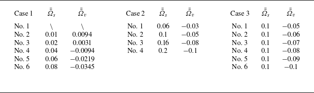
1. Introduction
The investigation of swirling flow phenomena holds a prominent position in fluid mechanics (see Zandbergen & Dijkstra Reference Zandbergen and Dijkstra1987; Gallaire & Chomaz Reference Gallaire and Chomaz2003; Douglas, Emerson & Lieuwen Reference Douglas, Emerson and Lieuwen2022), with the research progressing primarily along two distinct directions. The first one focuses on elucidating the influence of swirling flows on flow stability, encompassing phenomena such as vortex breakdown, hysteresis, turbulence-induced axisymmetry breakdown (Gelfgat, Bar-Yoseph & Solan Reference Gelfgat, Bar-Yoseph and Solan1996; Shtern & Hussain Reference Shtern and Hussain1999), dynamical characteristics of atmospheric circulation (Afanasyev & Peltier Reference Afanasyev and Peltier1998; Satoh Reference Satoh2004), and extreme natural vortices including tornadoes (Nolan Reference Nolan2012; Rotunno Reference Rotunno2013) and fire whirls (Emmons & Ying Reference Emmons and Ying1967; Battaglia, Rehm & Baum Reference Battaglia, Rehm and Baum2000; Zhou & Wu Reference Zhou and Wu2007). The second examines how swirling background flows modulate the propagation characteristics of disturbance waves, specifically acoustic, vortical and entropic modes (Kousen Reference Kousen1995; Golubev & Atassi Reference Golubev and Atassi1998; Tam & Auriault Reference Tam and Auriault1998; Heaton & Peake Reference Heaton and Peake2005; Posson & Peake Reference Posson and Peake2013b ; Mathews & Peake Reference Mathews and Peake2017). Building on foundational principles into wave dynamics in complex flows, the acoustic analogy theory presented by Lighthill (Reference Lighthill1952) has been extended to incorporate swirling effects (Posson & Peake Reference Posson and Peake2013a ), establishing a novel theoretical framework for aeroacoustic research (Posson & Peake Reference Posson and Peake2013b ; Masson et al. Reference Masson, Mathews, Moreau, Posson and Brambley2018). Both research directions share a common emphasis on multiscale (temporal and spatial scales) energy transfer mechanisms, emphasizing either disturbance amplification (instability) or the generation and evolution of modal disturbances (propagation).
Notably, a distinct energy transfer mechanism involving thermoacoustic coupling, i.e. the interaction between unsteady heat release and flow perturbations, has been recognized as a driver of thermoacoustic instabilities in a confined space. Recent applications of advanced swirlers in premixed combustion systems (Huang & Yang Reference Huang and Yang2009; Kim Reference Kim2016) and radial flameholders in afterburners (Lovett et al. Reference Lovett, Brogan, Philippona, Kiel and Thompson2004) have revealed susceptibility to intense azimuthal thermoacoustic oscillations under strong swirl conditions. These oscillations not only risk structural damage but also present challenges to existing thermoacoustic instability models, which inadequately account for high-swirl effects. However, thermoacoustic instability represents a global stability phenomenon governed by the interplay of flow, unsteady heat release and confined geometry. In view of its systemic nature, the role of swirling flows in modulating such instabilities remains understudied compared with extensive body of work dedicated to localized swirling flame dynamics (Huang & Yang Reference Huang and Yang2009; Durox et al. Reference Durox, Moeck, Bourgouin, Morenton, Viallon, Schuller and Candel2013; Candel et al. Reference Candel, Durox, Schuller, Bourgouin and Moeck2014) and the fundamental swirling flow instability mechanisms in fluid mechanics. Furthermore, in contrast to conventional ways of suppressing thermoacoustic instabilities, the effective control of thermoacoustic instability under conditions of strong swirling flows has emerged as an urgent challenge for various industrial applications. Naturally, these concerns are largely contingent upon gaining insights into the interaction mechanisms between unsteady heat release and swirling flows, as well as quantitatively characterizing their effects on the onset of thermoacoustic instability. Our interest herein is to focus upon the characteristics of thermoacoustic instabilities in swirling flow configurations.
Recent studies have attempted to investigate the influence of swirling flows on azimuthal thermoacoustic instabilities. In theoretical modelling, initial efforts concentrated on extending network models and three-dimensional Helmholtz solvers, originally developed for longitudinal instabilities, to predict azimuthal modes (Dowling Reference Dowling1995; Evesque & Polifke Reference Evesque and Polifke2002; Lieuwen & Yang Reference Lieuwen and Yang2005; Nicoud et al. Reference Nicoud, Benoit, Sensiau and Poinsot2007). Subsequent refinements incorporated circumferential mean flow effects while satisfying azimuthal periodic boundary conditions (Bauerheim, Cazalens & Poinsot Reference Bauerheim, Cazalens and Poinsot2015; Faure-Beaulieu, Pedergnana & Noiray Reference Faure-Beaulieu, Pedergnana and Noiray2023). These investigations demonstrate that the azimuthal instabilities can manifest as standing or spinning modes, with dynamical transitions between these states observed under specific conditions (Evesque, Polifke & Pankiewitz Reference Evesque, Polifke and Pankiewitz2003; Schuermans, Paschereit & Monkewitz Reference Schuermans, Paschereit and Monkewitz2006; Qin et al. Reference Qin, Wang, Zhang and Sun2025). Additionally, the research analyses the mechanism of symmetry breaking induced by circumferential mean swirling flows. Experimental and numerical simulations further corroborate these analytical findings (Krebs et al. Reference Krebs, Flohr, Prade and Hoffmann2002; Wolf et al. Reference Wolf, Staffelbach, Gicquel, Müller and Poinsot2012; Worth & Dawson Reference Worth and Dawson2013). In numerical simulations, large eddy simulation techniques have been applied to analyse the effect of swirling flows on the localized combustion instability related to flame dynamics (Stone & Menon Reference Stone and Menon2002; Urbano et al. Reference Urbano, Selle, Staffelbach, Cuenot, Schmitt, Ducruix and Candel2016; Zhang et al. Reference Zhang, Shahsavari, Rao, Yang and Wang2021).
However, the existing methods universally approximate the circumferential mean velocity as uniform (Bauerheim et al. Reference Bauerheim, Cazalens and Poinsot2015; Li et al. Reference Li, Yang, Li and Zhu2019), neglecting the radial dependence of axial and circumferential velocity components inherent to realistic swirling flows. This simplification precludes a systematic understanding of how radial velocity gradients modulate azimuthal thermoacoustic instabilities as a three-dimensional problem associated with acoustic resonance in a confined space. Notably, most theoretical and experimental studies have established that non-uniform flow profiles critically influence flow stability and wave propagation phenomena (Posson & Peake Reference Posson and Peake2013a ; Douglas et al. Reference Douglas, Emerson and Lieuwen2022). By analogy, it is reasonable to believe that radial velocity gradients in swirling flows likely constitute critical parameters affecting thermoacoustic instability, necessitating their explicit incorporation into models.
Ultimately, thermoacoustic instability fundamentally arises from the coupling between unsteady heat release, flow dynamics and acoustic fields. To integrate these mechanisms into thermoacoustic models, a systematic approach is required. In this context, it is necessary to focus on the modal analysis of the flow field, followed by a comprehensive investigation of how swirling flows affect wave propagation within a confined space. The study of small-amplitude disturbances in ducted flows emerged in earnest during the 1960s. For uniform or non-uniform flow but no swirl configurations, significant research is available, such as analysis of spinning acoustic modes in uniform throughflows (Tyler & Sofrin Reference Tyler and Sofrin1962; Sun et al. Reference Sun, Wang, Du and Sun2022; Shen et al. Reference Shen, Wang, Sun, Zhang and Sun2022) and investigations of duct modes under non-uniform velocity profiles (Pridmore-Brown Reference Pridmore-Brown1958; Mungar & Plumblee Reference Mungar and Plumblee1969; Shankar Reference Shankar1972; Unruh & Eversman Reference Unruh and Eversman1972; Ko Reference Ko1973; Nayfeh, Kaiser & Telionis Reference Nayfeh, Kaiser and Telionis1975; Swinbanks Reference Swinbanks1975). In swirling flow contexts, the propagation of small-amplitude disturbances has been investigated by Kerrebrock (Reference Kerrebrock1974, Reference Kerrebrock1977), Goldstein (Reference Goldstein1978), Golubev & Atassi (Reference Golubev and Atassi1995), Golubev & Atassi (Reference Golubev and Atassi1997) and Mathews & Peake (Reference Mathews and Peake2017). Notably, Kousen (Reference Kousen1995, Reference Kousen1996) established a systematic methodology for analysing small-amplitude wave modes in inviscid, compressible swirling flows in an annulus using normal mode decomposition and eigenvalue analysis. Collectively, these studies clarify the mechanisms of disturbance generation and evolution in a confined space with complex flow environments.
Moreover, in contrast to uniform flow scenarios, where disturbance mode formation, conversion and propagation follow well-established dynamics, non-uniform flows (e.g. shear flows, swirling flows) exhibit distinct modal behaviours. These variations of propagating modes directly modify resonant characteristics in the confined space, thereby altering prediction and evaluation of thermoacoustic instability. Recent work by Albayrak, Juniper & Polifke (Reference Albayrak, Juniper and Polifke2019) demonstrated that when a plane wave interacts with swirling flows within a combustor swirl burner, `inertial waves’ are generated. Furthermore, they identified that azimuthal velocity perturbations in swirling flows can be classified as dispersive inertial waves, which provides a more comprehensive explanation for the existing experimental observations related to azimuthal perturbations. Therefore, it is intuitively reasonable to believe that incorporating the effects of swirling flows throughout the entire combustion system, rather than limiting the analysis to the localized burner regions, may yield new insights into the coupling mechanisms between thermoacoustic instability and swirling flows, which currently remains an open question.
In terms of the context, it is necessary to capture more swirling flow features to establish a more accurate predictive model for azimuthal thermoacoustic instability in the presence of swirling flows. In ducted swirling flows, it is important to accurately and comprehensively describe three physical mechanisms associated with wave motions: (i) fluid compressibility driving acoustic modes; (ii) centrifugal forces arising from the rotational motion of the mean flow; (iii) axially propagating wave modes corresponding to centrifugal force fields. In general, it is found that shear gradients of the mean velocity distribution can result in the propagation of shear waves in certain circumstances (Golubev & Atassi Reference Golubev and Atassi1997; Kousen Reference Kousen1999). In inviscid flow, it is well known that the presence of an inflection point in the velocity profile can lead to Kelvin–Helmholtz instability (Drazin & Reid Reference Drazin and Reid2004). However, in typical aerospace propulsion systems, it is reasonable to assume that the mean flow remains monotonic and stable. In view of the scales relevant to thermoacoustic oscillations, this work will comprehensively analyse and discuss the formation and propagation of acoustic waves, without emphasizing the waves generated by velocity gradients.
Building on the considerations detailed above, we will begin by applying the compressible linearized Euler equations, as utilized by Kousen (Reference Kousen1999), while assuming that the mean swirling flows exhibit either solid body rotation or free vortex behaviour. However, we encounter two significant theoretical challenges that must be addressed. First, conventional swirling flow models typically assume an infinite-length solution domain, with a primary focus on the impact of swirling flows on wave motion. Consequently, it is critical to derive the fundamental equations and obtain their solutions within a confined space, characterized by complex inlet and outlet boundary conditions that represent a realistic combustion chamber, as there is a lack of similar work addressing swirling flows in finite domains. Second, it is essential to determine how to effectively couple with an unsteady heat release model to form a physically reasonable energy conversion mechanism among the flow dynamics, acoustic fields and heat responses.
To address the first challenge, we develop a standing-wave solution incorporating inlet and outlet boundary conditions, thereby reducing the three-dimensional partial differential equation to a radial ordinary differential equation via axial standing-wave decomposition and circumferential harmonic hypothesis. This process constructs radial-dependent flow-acoustic equations within a finite-length domain. For the second challenge, energy equations and flame response models are systematically integrated with linearized Euler equations at the inlet of combustion chamber to establish coupled thermoacoustic energy exchange. These approaches yield a radial ordinary differential equation coupled with unsteady heat release, enabling derivation of an eigenvalue matrix equation for swirling flows within confined spaces.
Validation demonstrates agreement with both infinite-domain swirling flow benchmarks and mode-matching standing-wave solutions for thermoacoustic analysis. Moreover, the model reveals certain valuable insights into swirl-thermoacoustic coupling mechanisms. The remainder of this paper is structured as follows. Section 2 develops a three-dimensional framework for analysing thermoacoustic instability by integrating radially dependent swirling flow profiles, unsteady heat release dynamics and outlet boundary conditions into the linearized Euler equations. This section details the derivation of characteristic equations incorporating radial velocity gradients and outlines their numerical resolution. The model is validated in § 3 through comparative analysis of acoustic-wave propagation in radial non-uniform flow fields and thermoacoustic instability under uniform flow conditions, demonstrating predictive consistency. Section 4 employs parametric analysis on a model annular combustor to quantify the distinct effects of radially independent versus radially dependent velocity profiles on oscillation frequencies and growth rates for azimuthal modes. Results indicate the pivotal role of swirling velocity in governing thermoacoustic modal transition dynamics. Finally, § 5 provides a comprehensive summary of the research results.
Sketch of swirling flows in the combustor.

2. Thermoacoustic instability with radially dependent swirling flows and flame responses in a confined combustion chamber
Figure 1 illustrates a typical combustion chamber featuring 12 evenly distributed burners at the inlet. While the effects of swirling flows on inertial waves in the burners have been thoroughly investigated in prior studies (Albayrak et al. Reference Albayrak, Juniper and Polifke2019), this work does not focus on the swirling flows within the burners themselves. Instead, drawing on the assumption made by Bauerheim et al. (Reference Bauerheim, Cazalens and Poinsot2015) that only plane waves propagate within the narrow burners, we concentrate on the impact of radially dependent swirling flows in the combustion chamber on azimuthal thermoacoustic instabilities. It is important to note that our analysis is based on an annular combustion chamber with a relatively large hub ratio, selected to facilitate validation against existing results (Bauerheim et al. Reference Bauerheim, Cazalens and Poinsot2015). This methodology is also applicable to combustion chambers with smaller hub ratios, such as can-type combustors, where enhanced radial non-uniformity is anticipated.
To capture the coupling effect of the flame and swirling flows within the combustion chamber on thermoacoustic instabilities, some simplifying assumptions are necessary. Specifically, viscosity, heat conduction and additional mass and force source terms are neglected, and the isentropic condition is assumed. Consequently, the governing equations in the combustion chamber are represented by the unsteady Euler equations. Thus, the equations of continuity and momentum are written as
 \begin{align} \frac {\partial \rho }{\partial t} + \bigtriangledown \boldsymbol{\cdot }\left ( \rho \boldsymbol{u} \right ) &= 0, \end{align}
 \begin{align} \rho \frac {\partial \boldsymbol{u}}{\partial t} + \bigtriangledown p &= 0, \end{align}
where
 $\rho$
,
 $\boldsymbol{u}$
,
 $p$
and
 $t$
represent density, velocity vector, pressure and time, respectively, with
 $\boldsymbol{u}=u_\theta (r) \boldsymbol{n}_{\theta } + u_r(r) \boldsymbol{n}_r + u_x(r) \boldsymbol{n}_x$
. The components
 $u_\theta$
,
 $u_r$
and
 $u_x$
represent the velocities in the circumferential, radial and axial directions, respectively, under cylindrical coordinate denoted by
 $\boldsymbol{n}_{\theta }$
,
 $\boldsymbol{n}_r$
and
 $\boldsymbol{n}_x$
(labelled by
 $\theta$
,
 $r$
and
 $x$
). The bold character denotes the vector. Under the linear assumption, the density, velocity and pressure in (2.1) and (2.2) are expressed as the sum of the mean quantities
 $\bar {()}$
and the first-order perturbations
 $\tilde {()}$
, when neglecting second-order perturbations and the unsteady terms of the mean quantities. Consequently, the governing equations of the mean quantities and the first-order perturbations can be derived. To clarify, the equations for mean quantities and perturbations under swirling flows are detailed in §§ 2.1 and 2.2, respectively.
2.1. Radially dependent mean quantities in an annular duct with swirling flows
If the mean field in the combustion chamber is uniform, i.e. uniform axial mean flow and uniform circumferential mean flow, the quantities of mean pressure, mean density, sound speed and so on in the combustion chamber can be obtained, according to the ideal gas state equation. However, the presence of centrifugal forces resulting from the swirling flows causes the mean pressure, mean density and sound speed are radially dependent. Wherein the mean pressure is governed by the radial momentum equation (see (2.2)), which under the simplified condition can be expressed as
 \begin{equation} \frac {\textrm{d} \bar {p}}{\textrm{d} r} = \frac {\bar {\rho } \bar {u}_\theta ^2}{r}, \end{equation}
where
 $\bar {u}_\theta$
represents the circumferential mean velocity. Under the assumptions of isentropy and constant specific heat, the relationships
 $\textrm{d}\bar {p}/\textrm{d} r = \bar {c}^2 \textrm{d} \bar {\rho }/\textrm{d} r$
and
 $\bar {c}^2 = \gamma \bar {p}/\bar {\rho }$
are satisfied between the mean pressure
 $\bar {p}$
, mean density
 $\bar {\rho }$
and sound speed
 $\bar {c}$
for ideal gas, with
 $\gamma$
representing the specific heat ratio. Therefore, the sound speed in the radial direction can then be determined by further solving the radial momentum equation for the mean quantities, which is expressed as
 \begin{equation} \frac {\textrm{d} \bar {c}}{\textrm{d} r} = \left (\gamma -1\right ) \frac {\bar {u}_\theta ^2}{2r\bar {c}}. \end{equation}
By integrating along the radial direction, the sound speed can be obtained by further solving (2.4), yielding
 \begin{equation} \bar {c}^2(r) = \bar {c}^2(r_t) - \left (\gamma -1\right ) \int _r^{r_t} \frac {\bar {u}_\theta ^2}{r} \textrm{d} r, \end{equation}
where
 $r_t$
represents the outer radius of the duct. This means that once the radial distribution of circumferential mean velocity is obtained, the radial distribution of the sound speed can be obtained by the integral equation of (2.5). In general, two types of classical swirling flows are typically considered in the combustion chamber: solid body swirl and free vortex swirl. According to Kerrebrock (Reference Kerrebrock1974, Reference Kerrebrock1977), solid body swirl represents the flow behind a high-work blade row, while it coexists with free vortex swirl to model the flow behind a rotor. For the circumferential velocity at any radial position in the practical device, in a simplified case, it can be considered that the circumferential mean velocity consists of these two kinds of swirl. Then the circumferential mean velocity can be mathematically expressed as
 \begin{align} \bar {u}_{\theta ,sb} &= \varOmega _s r, \end{align}
 \begin{align} \bar {u}_{\theta ,fv} &= \frac {\varOmega _v}{r}, \end{align}
 \begin{align} \bar {u}_{\theta ,sb,fv} &= \varOmega _s r + \frac {\varOmega _v}{r}, \end{align}
where
 $\bar {u}_{\theta ,sb}$
and
 $\bar {u}_{\theta ,fv}$
denote the circumferential mean velocity under the conditions of solid body swirl and free vortex swirl, respectively. Here,
 $\bar {u}_{\theta ,sb,fv}$
represents the circumferential mean velocity resulting from both swirling conditions. Here
 $\varOmega _s$
and
 $\varOmega _v$
satisfy
 $\varOmega _s=\bar {\bar {\varOmega }}_s \bar {c}({r_t})/{r_t}$
and
 $\varOmega _v=\bar {\bar {\varOmega }}_v \bar {c}({r_t}){r_t}$
, with
 $\bar {\bar {\varOmega }}_s$
and
 $\bar {\bar {\varOmega }}_v$
representing the normalized angular velocity of the solid body swirl and the strength of the free vortex swirl, respectively. By combining (2.5) and (2.6) and integrating along the radial direction, the sound speed under the condition of the three typical circumferential mean velocities can be derived as
 \begin{align} \bar {c}^2(r) = \bar {c}^2(r_t) &- \frac {\gamma -1}{2} \varOmega _s^2 \big (r_t^2-r^2\big ), \end{align}
 \begin{align} \bar {c}^2(r) = \bar {c}^2(r_t) &- \frac {\gamma -1}{2} \varOmega _v^2 \left (\frac {1}{r^2}-\frac {1}{r_t^2}\right ), \end{align}
 \begin{align} \bar {c}^2(r) = \bar {c}^2(r_t) - \frac {\gamma -1}{2} & \left [\varOmega _s^2 \big (r_t^2-r^2\big ) +\varOmega _v^2 \left (\frac {1}{r^2}-\frac {1}{r_t^2}\right ) \right ] +2(\gamma -1) \varOmega _s \varOmega _v \textrm{ln}\left(\frac {r}{r_t}\right). \end{align}
Under the isentropic assumption, the relationships
 $\bar {\bar {c}}^2 =\bar {\bar {p}} / \bar {\bar {\rho }}$
and
 $\bar {\bar {p}} = \bar {\bar {\rho }} ^ {\gamma }$
hold, with
 $\bar {\bar {c}}(r)=\bar {c}(r)/\bar {c}(r_t)$
,
 $\bar {\bar {p}}(r)=\bar {p}(r)/\bar {p}(r_t)$
and
 $\bar {\bar {\rho }}(r)=\bar {\rho }(r)/\bar {\rho }(r_t)$
. Consequently, the radially dependent mean density and mean pressure can be expressed as
 \begin{align} \bar {\bar {\rho }}(r) &= \left [\bar {\bar {c}}^2(r)\right ]^{\frac {1}{\gamma -1}}, \end{align}
 \begin{align} \bar {\bar {p}}(r) &= \left [\bar {\bar {c}}^2(r)\right ]^{\frac {\gamma }{\gamma -1}}. \end{align}
Therefore, distinguishing mean quantities for uniform conditions, the radially dependent mean quantities are obtained as presented in (2.7)–(2.9) caused by swirling flows.
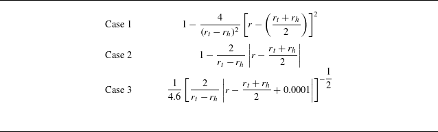
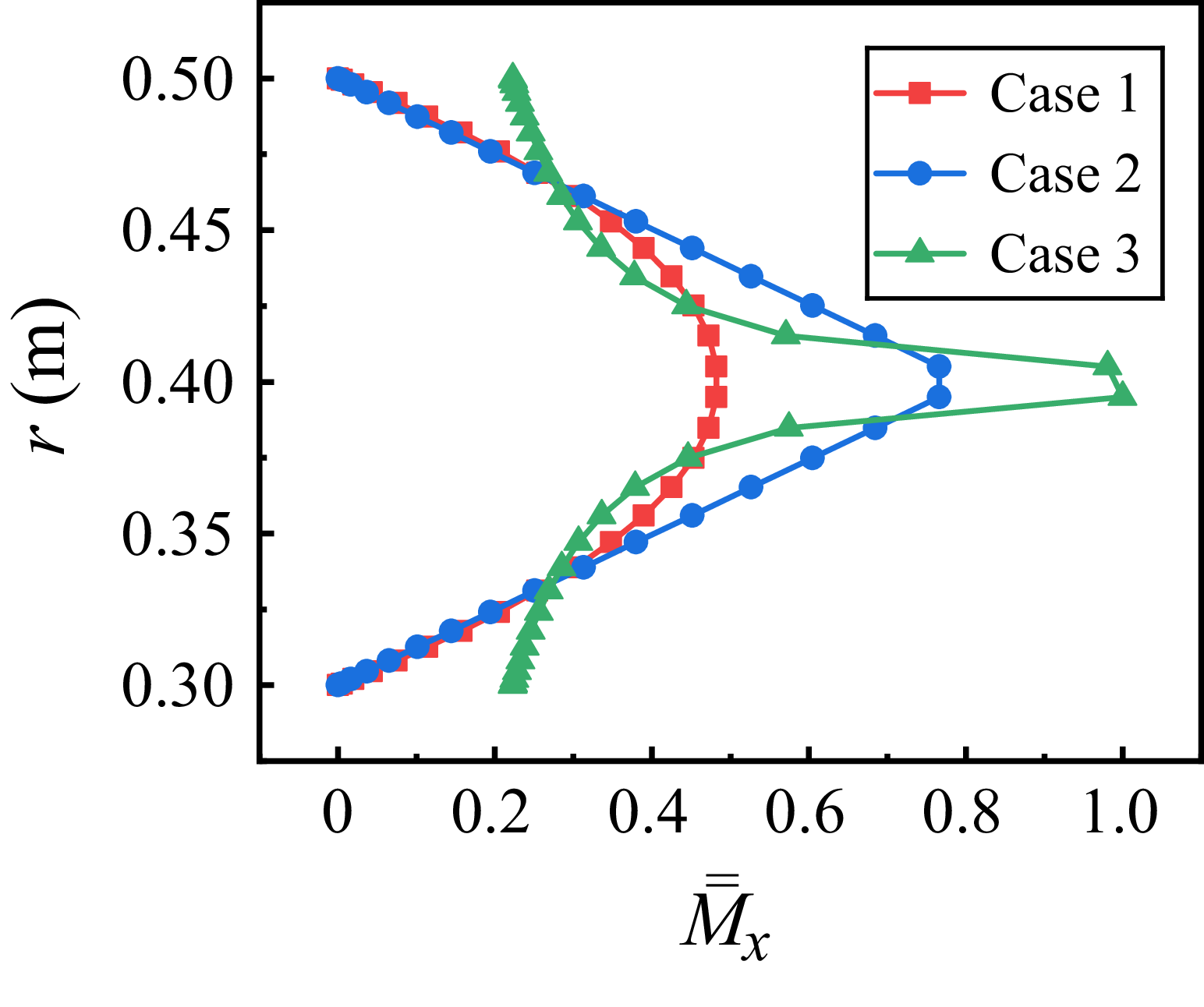
In reality, combustion chambers exhibit complex radially non-uniform flows, including variations in swirl intensity. These configurations can also be analysed within this framework. However, this work specifically employs radially independent swirls in (2.6) for several reasons: first, it facilitates direct comparison with existing studies at fixed swirls while incorporating radial-dependent mean flow fields (Kousen Reference Kousen1995; Nijboer Reference Nijboer2001); second, it allows for an analytical solution of the radially dependent mean parameters influenced by swirl-induced centrifugal forces.
2.2. Linearized Euler equations tailored to the finite-length annular duct
In addition to the radially dependent mean quantities affected by the swirling flows, if the mean quantities are uniform, then the first-order unsteady quantities satisfy the Helmholtz equation in a three-dimensional space and thus the unsteady perturbations can be obtained theoretically. It can be found in § 2.1 that, the mean quantities are radially dependent with the effect of swirling flows. This causes the unsteady perturbations not be able to be obtained theoretically under the non-uniform field; consequently, this section will present the radially dependent perturbations subject to swirling flows, as illustrated in figure 2. The radial mean velocity
 $\bar {u}_r$
is assumed negligible and the mean circumferential and axial velocities (
 $\bar {u}_\theta$
and
 $\bar {u}_x$
) remain constant in the circumferential and axial directions. The governing equations for the first-order perturbations can be simplified by neglecting the effects of the second-order and higher-order perturbations in cylindrical coordinates. With the condition of
 $\tilde {\rho }= \tilde {p}/\bar {c}^2$
under the assumption of isentropic flow, the governing equations for the perturbations are expressed as
Sketch of perturbations in the combustion chamber.

 \begin{align} \frac {1}{\bar {c}_c^2} \left (\frac {\partial }{\partial t} + \frac {\bar {u}_\theta }{r} \frac {\partial }{\partial \theta } + \bar {u}_x \frac {\partial }{\partial x} \right ) \tilde {p}_c &+ \left (\bar {\rho }_c \frac {\partial }{\partial r} + \frac {\bar {\rho }_c}{r} + \frac {\partial \bar {\rho }_c}{\partial r} \right ) \tilde {u}_r + \frac {\bar {\rho }_c}{r} \frac {\partial \tilde {u}_\theta }{\partial \theta } + \bar {\rho }_c \frac {\partial \tilde {u}_x}{\partial x} = 0, \\[-28pt] \nonumber \end{align}
 \begin{align} \left (\frac {\partial }{\partial r} - \frac {\bar {u}_\theta ^2}{\bar {c}_c^2 r} \right ) \tilde {p}_c &+ \left (\bar {\rho }_c \frac {\partial }{\partial t} + \frac {\bar {\rho }_c \bar {u}_\theta }{r} \frac {\partial }{\partial \theta } + \bar {\rho }_c \bar {u}_x \frac {\partial }{\partial x} \right ) \tilde {u}_r - \frac {2 \bar {\rho }_c \bar {u}_\theta }{r} \tilde {u}_\theta = 0, \\[-28pt] \nonumber \end{align}
 \begin{align} \frac {1}{r} \frac {\partial \tilde {p}_c}{\partial \theta } + \left (\bar {\rho }_c \frac {\partial \bar {u}_\theta }{\partial r} + \frac {\bar {\rho }_c \bar {u}_\theta }{r} \right ) \tilde {u}_r &+ \left (\bar {\rho }_c \frac {\partial }{\partial t} + \frac {\bar {\rho }_c \bar {u}_\theta }{r} \frac {\partial }{\partial \theta } + \bar {\rho }_c \bar {u}_x \frac {\partial }{\partial x} \right ) \tilde {u}_\theta = 0, \\[-28pt] \nonumber \end{align}
 \begin{align} \frac {\partial \tilde {p}_c}{\partial x} + \bar {\rho }_c \frac {\partial \bar {u}_x}{\partial r} \tilde {u}_r &+ \left (\bar {\rho }_c \frac {\partial }{\partial t} + \frac {\bar {\rho }_c \bar {u}_\theta }{r} \frac {\partial }{\partial \theta } + \bar {\rho }_c \bar {u}_x \frac {\partial }{\partial x} \right ) \tilde {u}_x = 0, \\[0pt] \nonumber \end{align}
where the subscript ‘
 $c$
’ denotes the parameters related to the combustion chamber. With the harmonic assumption and modal expansion, the perturbations in the above equations can be expressed as the function of
 $\textrm{e}^{{\rm i} (\omega t - \kappa _x x + m \theta )}$
. Wherein
 ${\rm i}$
is the imaginary unit,
 $\omega$
represents the complex frequency,
 $\kappa _x$
denotes the axial wavenumber and
 $m$
indicates the azimuthal mode number. As depicted in figure 2, the combustion chamber, which features a finite axial length, contains two sets of acoustic waves propagating in both upstream and downstream directions. These acoustic waves are influenced by the interfaces between the combustion chamber inlet and the burners (
 $x_b{-}x_b$
interface), as well as by the outlet boundary conditions of the combustion chamber (
 $x_c{-}x_c$
interface) in figure 2. Then the unsteady perturbations can be expressed as
 \begin{align} \tilde {p}_c &= \sum _{m=-\infty }^{\infty } \textrm{e}^{{\rm i} (\omega t - \kappa _{x,m}^+ x + m \theta )} \hat {p}_m^+ + \textrm{e}^{{\rm i} (\omega t - \kappa _{x,m}^- x + m \theta )} \hat {p}_m^-, \end{align}
 \begin{align} \tilde {u}_r &= \sum _{m=-\infty }^{\infty } \textrm{e}^{{\rm i} (\omega t - \kappa _{x,m}^+ x + m \theta )} \hat {u}_{r,m}^+ + \textrm{e}^{{\rm i} (\omega t - \kappa _{x,m}^- x + m \theta )} \hat {u}_{r,m}^-, \end{align}
 \begin{align} \tilde {u}_\theta &= \sum _{m=-\infty }^{\infty } \textrm{e}^{{\rm i} (\omega t - \kappa _{x,m}^+ x + m \theta )} \hat {u}_{\theta ,m}^+ + \textrm{e}^{{\rm i} (\omega t - \kappa _{x,m}^- x + m \theta )} \hat {u}_{\theta ,m}^-, \end{align}
 \begin{align} \tilde {u}_x &= \sum _{m=-\infty }^{\infty } \textrm{e}^{{\rm i} (\omega t - \kappa _{x,m}^+ x + m \theta )} \hat {u}_{x,m}^+ + \textrm{e}^{{\rm i} (\omega t - \kappa _{x,m}^- x + m \theta )} \hat {u}_{x,m}^-, \end{align}
where superscripts ‘+’ and ‘
 $-$
’ represent the perturbations propagating downstream and upstream, respectively, and superscript
 $ \hat {()}$
denotes the complex amplitude. Specifically,
 $\kappa _{x,m}^+$
and
 $\kappa _{x,m}^-$
represent the axial wavenumber propagating downstream and upstream for azimuthal mode ‘
 $m$
’, respectively. The complex pressure amplitude correspond to downstream and upstream propagation are given by
 $\hat {p}_m^+$
and
 $\hat {p}_m^-$
. Similarly, the complex velocity amplitude for downstream and upstream propagation in the radial, circumferential and axial directions are denoted as
 $\hat {u}_{r,m}^+$
and
 $\hat {u}_{r,m}^-$
,
 $\hat {u}_{\theta ,m}^+$
and
 $\hat {u}_{\theta ,m}^-$
,
 $\hat {u}_{x,m}^+$
and
 $\hat {u}_{x,m}^-$
, respectively. Inserting (2.14) into (2.10)–(2.13) allows the partial differential equations to be reduced to ordinary differential equations in the radial direction, which is radially dependent and expressed as
 \begin{align} &\sum _{m=-\infty }^{\infty } \frac {\textrm{i}}{\bar {c}_c^2 r} \left (\zeta ^+ \textrm{e}^{-{\rm i} \kappa _{x,m}^+ x} \hat {p}_m^+ + \zeta ^- \textrm{e}^{-{\rm i} \kappa _{x,m}^- x} \hat {p}_m^- \right ) \textrm{e}^{{\rm i} (\omega t + m \theta )} \nonumber\\& + \sum _{m=-\infty }^{\infty } \left (\bar {\rho }_c \frac {\textrm{d}}{\textrm{d} r} + \frac {\bar {\rho }_c}{r} + \frac {\textrm{d} \bar {\rho }_c}{\textrm{d} r} \right ) \left (\textrm{e}^{-{\rm i} \kappa _{x,m}^+ x} \hat {u}_{r,m}^+ + \textrm{e}^{-{\rm i} \kappa _{x,m}^- x} \hat {u}_{r,m}^-\right ) \textrm{e}^{{\rm i} (\omega t + m \theta )} \nonumber\\& + \sum _{m=-\infty }^{\infty } {\rm i} m \frac {\bar {\rho }_c}{r} \left (\textrm{e}^{-{\rm i} \kappa _{x,m}^+ x} \hat {u}_{\theta ,m}^+ + \textrm{e}^{-{\rm i} \kappa _{x,m}^- x} \hat {u}_{\theta ,m}^-\right ) \textrm{e}^{{\rm i} (\omega t + m \theta )} \nonumber\\& - \sum _{m=-\infty }^{\infty } \textrm{i} \bar {\rho }_c \left (\kappa _{x,m}^+ \textrm{e}^{-{\rm i} \kappa _{x,m}^+ x} \hat {u}_{x,m}^+ + \kappa _{x,m}^- \textrm{e}^{-{\rm i} \kappa _{x,m}^- x} \hat {u}_{x,m}^-\right ) \textrm{e}^{{\rm i} (\omega t + m \theta )} =0, \end{align}
 \begin{align} & \sum _{m=-\infty }^{\infty } \left (\frac {\textrm{d}}{\textrm{d}r} - \frac {\bar {u}_\theta ^2}{\bar {c}_c^2 r} \right ) \left (\textrm{e}^{-{\rm i} \kappa _{x,m}^+ x} \hat {p}_m^+ + \textrm{e}^{-{\rm i} \kappa _{x,m}^- x} \hat {p}_m^- \right ) \textrm{e}^{{\rm i} (\omega t + m \theta )} \nonumber\\ & + \sum _{m=-\infty }^{\infty } \frac {\textrm{i} \bar {\rho }_c}{r} \left (\zeta ^+ \textrm{e}^{-{\rm i} \kappa _{x,m}^+ x} \hat {u}_{r,m}^+ + \zeta ^- \textrm{e}^{-{\rm i} \kappa _{x,m}^- x} \hat {u}_{r,m}^-\right ) \textrm{e}^{{\rm i} (\omega t + m \theta )} \nonumber\\ & - \sum _{m=-\infty }^{\infty } \frac {2 \bar {\rho }_c \bar {u}_\theta }{r} \left (\textrm{e}^{-{\rm i} \kappa _{x,m}^+ x} \hat {u}_{\theta ,m}^+ + \textrm{e}^{-{\rm i} \kappa _{x,m}^- x} \hat {u}_{\theta ,m}^- \right ) \textrm{e}^{{\rm i} (\omega t + m \theta )} = 0, \end{align}
 \begin{align} & \sum _{m=-\infty }^{\infty } \frac {{\rm i} m}{r} \left (\textrm{e}^{-{\rm i} \kappa _{x,m}^+ x} \hat {p}_m^+ + \textrm{e}^{-{\rm i} \kappa _{x,m}^- x} \hat {p}_m^-\right ) \textrm{e}^{{\rm i} (\omega t + m \theta )} \nonumber\\ & + \sum _{m=-\infty }^{\infty } \bar {\rho }_c \left (\frac {\textrm{d} \bar {u}_\theta }{\textrm{d} r} + \frac {\bar {u}_\theta }{r} \right ) \left (\textrm{e}^{-{\rm i} \kappa _{x,m}^+ x} \hat {u}_{r,m}^+ + \textrm{e}^{-{\rm i} \kappa _{x,m}^- x} \hat {u}_{r,m}^-\right ) \textrm{e}^{{\rm i} (\omega t + m \theta )} \nonumber\\ & + \sum _{m=-\infty }^{\infty } \frac {{\rm i}\bar {\rho }_c}{r} \left (\zeta ^+ \textrm{e}^{-{\rm i} \kappa _{x,m}^+ x} \hat {u}_{\theta ,m}^+ + \zeta ^- \textrm{e}^{-{\rm i} \kappa _{x,m}^- x} \hat {u}_{\theta ,m}^-\right ) \textrm{e}^{{\rm i} (\omega t + m \theta )} = 0, \end{align}
 \begin{align} & \sum _{m=-\infty }^{\infty } \textrm{i} \left (\kappa _{x,m}^+ \textrm{e}^{-{\rm i} \kappa _{x,m}^+ x} \hat {p}_m^+ + \kappa _{x,m}^- \textrm{e}^{-{\rm i} \kappa _{x,m}^- x} \hat {p}_m^-\right ) \textrm{e}^{{\rm i} (\omega t + m \theta )} \nonumber\\ & - \sum _{m=-\infty }^{\infty } \bar {\rho }_c \frac {\textrm{d} \bar {u}_x}{\textrm{d} r} \left (\textrm{e}^{-{\rm i} \kappa _{x,m}^+ x} \hat {u}_{r,m}^+ + \textrm{e}^{-{\rm i} \kappa _{x,m}^- x} \hat {u}_{r,m}^-\right ) \textrm{e}^{{\rm i} (\omega t + m \theta )} \nonumber\\ & - \sum _{m=-\infty }^{\infty } \frac {\textrm{i}\bar {\rho }_c}{r} \left (\zeta ^+ \textrm{e}^{-{\rm i} \kappa _{x,m}^+ x} \hat {u}_{x,m}^+ +\zeta ^- \textrm{e}^{-{\rm i} \kappa _{x,m}^- x} \hat {u}_{x,m}^-\right ) \textrm{e}^{{\rm i} (\omega t + m \theta )} = 0, \end{align}
with
 \begin{align} \zeta ^+ = \omega r + m \bar {u}_\theta - \kappa _{x,m}^+ \bar {u}_x r, \end{align}
 \begin{align} \zeta ^- = \omega r + m \bar {u}_\theta - \kappa _{x,m}^- \bar {u}_x r. \end{align}
Equations (2.15)–(2.18) show that the perturbations are solely radially dependent, thus making it the ordinary differential equation in the radial direction. To further simplify the modal expression in the circumferential direction, we multiply
 $\textrm{e}^{-{\rm i} m' \theta }$
and integrate along the circumference on the both sides of the (2.15)–(2.18). Considering
 $\int _0^{2 \pi } \textrm{e}^{{\rm i} (m-m' ) \theta } \textrm{d} \theta = 2 \pi f_{\delta (m, m')}$
, where
 $f_{\delta (m, m')}$
is Kronecker delta function, then the governing equations of the unsteady flow, i.e. (2.15)–(2.18), can be obtained by further multiplying the radius
 $r$
, which is
 \begin{align} & \frac {\textrm{i}}{\bar {c}_c^2} \zeta ^+ \textrm{e}^{-{\rm i} \kappa _{x,m}^+ x} \hat {p}_m^+ + \frac {\textrm{i}}{\bar {c}_c^2} \zeta ^- \textrm{e}^{-{\rm i} \kappa _{x,m}^- x} \hat {p}_m^- + \left (\bar {\rho }_c r \frac {\textrm{d}}{\textrm{d} r} + \bar {\rho }_c + \frac {\textrm{d} \bar {\rho }_c}{\textrm{d} r} r \right ) \textrm{e}^{-{\rm i} \kappa _{x,m}^+ x} \hat {u}_{r,m}^+ \nonumber\\ & + \left (\bar {\rho }_c r \frac {\textrm{d}}{\textrm{d} r} + \bar {\rho }_c + \frac {\textrm{d} \bar {\rho }_c}{\textrm{d} r} r \right ) \textrm{e}^{-{\rm i} \kappa _{x,m}^- x} \hat {u}_{r,m}^- + {\rm i} m \bar {\rho }_c \textrm{e}^{-{\rm i} \kappa _{x,m}^+ x} \hat {u}_{\theta ,m}^+ + {\rm i} m \bar {\rho }_c \textrm{e}^{-{\rm i} \kappa _{x,m}^- x} \hat {u}_{\theta ,m}^- \nonumber\\ & - \textrm{i} \kappa _{x,m}^+ \bar {\rho }_c r \textrm{e}^{-{\rm i} \kappa _{x,m}^+ x} \hat {u}_{x,m}^+ - \textrm{i} \kappa _{x,m}^- \bar {\rho }_c r \textrm{e}^{-{\rm i} \kappa _{x,m}^- x} \hat {u}_{x,m}^- =0, \end{align}
 \begin{align} & \left (r \frac {\textrm{d}}{\textrm{d}r} - \frac {\bar {u}_\theta ^2}{\bar {c}_c^2} \right ) \textrm{e}^{-{\rm i} \kappa _{x,m}^+ x } \hat {p}_m^+ + \left (r \frac {\textrm{d}}{\textrm{d}r} - \frac {\bar {u}_\theta ^2}{\bar {c}_c^2} \right ) \textrm{e}^{-{\rm i} \kappa _{x,m}^- x} \hat {p}_m^- + \textrm{i} \bar {\rho }_c \zeta ^+ \textrm{e}^{-{\rm i} \kappa _{x,m}^+ x} \hat {u}_{r,m}^+ \nonumber\\ & + \textrm{i} \bar{\rho }_c \zeta ^- \textrm{e}^{-{\rm i} \kappa _{x,m}^- x} \hat {u}_{r,m}^- -2 \bar {\rho }_c \bar {u}_\theta \textrm{e}^{-{\rm i} \kappa _{x,m}^+ x} \hat {u}_{\theta ,m}^+ -2 \bar {\rho }_c \bar {u}_\theta \textrm{e}^{-{\rm i} \kappa _{x,m}^- x} \hat {u}_{\theta ,m}^- = 0, \end{align}
 \begin{align} & {\rm i} m \textrm{e}^{-{\rm i} \kappa _{x,m}^+ x} \hat {p}_m^+ + {\rm i} m \textrm{e}^{-{\rm i} \kappa _{x,m}^- x} \hat {p}_m^- + \left (\bar {\rho }_c r \frac {\textrm{d} \bar {u}_\theta }{\textrm{d} r} + \bar {\rho }_c \bar {u}_\theta \right ) \textrm{e}^{-{\rm i} \kappa _{x,m}^+ x} \hat {u}_{r,m}^+ \nonumber\\ & + \left (\bar {\rho }_c r \frac {\textrm{d} \bar {u}_\theta }{\textrm{d} r} + \bar {\rho }_c \bar {u}_\theta \right ) \textrm{e}^{- \textrm{i} \kappa _{x,m}^- x } \hat {u}_{r,m}^- + \textrm{i} \bar {\rho }_c \zeta ^+ \textrm{e}^{-{\rm i} \kappa _{x,m}^+ x} \hat {u}_{\theta ,m}^+ + \textrm{i} \bar {\rho }_c \zeta ^- \textrm{e}^{-{\rm i} \kappa _{x,m}^- x} \hat {u}_{\theta ,m}^- = 0, \end{align}
 \begin{align} & \textrm{i} \kappa _{x,m}^+ r \textrm{e}^{-{\rm i} \kappa _{x,m}^+ x} \hat {p}_m^+ + \textrm{i} \kappa _{x,m}^- r \textrm{e}^{-{\rm i} \kappa _{x,m}^- x} \hat {p}_m^- - \bar {\rho }_c r \frac {\textrm{d} \bar {u}_x}{\textrm{d} r} \textrm{e}^{-{\rm i} \kappa _{x,m}^+ x} \hat {u}_{r,m}^+ \nonumber\\ & - \bar {\rho }_c r \frac {\textrm{d} \bar {u}_x}{\textrm{d} r} \textrm{e}^{-{\rm i} \kappa _{x,m}^- x} \hat {u}_{r,m}^- - \textrm{i} \bar {\rho }_c \zeta ^+ \textrm{e}^{-{\rm i} \kappa _{x,m}^+ x} \hat {u}_{x,m}^+ - \textrm{i} \bar {\rho }_c \zeta ^- \textrm{e}^{-{\rm i} \kappa _{x,m}^- x} \hat {u}_{x,m}^- = 0. \end{align}
Therefore, the governing equations for perturbations with the effect of the swirling flows in the combustion chamber are presented in (2.20)–(2.23). Specifically, the axial wavenumber propagating upstream and downstream in the infinite-length duct under the influence of swirling flows can be determined based on the mean quantities.
2.3. Derivation of the inlet boundary conditions related to the burner flames
In addition to the governing equations for perturbations presented in § 2.2, the finite axial length of the combustion chamber necessitates that its inlet and outlet satisfy specific boundary conditions. As shown in figure 2, the outlet of the burners and the inlet of the combustion chamber align at the
 $x_b{-}x_b$
interface. Therefore, the inlet boundary condition of the combustion chamber is associated with the unsteady flame responses in the burners. Assuming that the combustion process occurs entirely within the burner, with a compact flame positioned at the burner outlet, the matching conditions of momentum and energy conservation equations for perturbations are thereby satisfied at the inlet of the combustion chamber, i.e. the
 $x_b{-}x_b$
interface. Under the isentropic assumption, the relationships
 $\tilde {\rho } = \tilde {p} / \bar {c}^2$
and
 $ c_p \tilde {T} = \tilde {p} / \bar {\rho }$
hold. This yields
 \begin{align} & \int _{\sum {S_f}} \left [\left (1+ \bar {M}_b^2\right ) \tilde {p}_b + 2\bar {\rho }_b \bar {u}_b \tilde {u}_b \right ] \textrm{d}S = \int _{S_c} \left [\left (1+ \bar {M}_x^2\right ) \tilde {p}_c + 2\bar {\rho }_c \bar {u}_x \tilde {u}_x \right ] \textrm{d}S, \end{align}
 \begin{align} & \int _{\sum {S_f}} \left [\tilde {q} + \left (\frac {\gamma \bar {u}_b}{\gamma -1} + \frac {\bar {M}_b^2 \bar {u}_b}{2}\right ) \tilde {p}_b + \left (\frac {\bar {\rho }_b \bar {c}_b^2}{\gamma -1} + \frac {3 \bar {\rho }_b \bar {u}_b^2}{2}\right ) \tilde {u}_b \right ] \textrm{d}S \nonumber\\ & = \int _{S_c} \left [\left (\frac {\gamma \bar {u}_x}{\gamma -1} + \frac {\bar {M}_x^2 \bar {u}_x}{2} + \frac {\bar {M}_\theta ^2 \bar {u}_x}{2}\right ) \tilde {p}_c + \left (\frac {\bar {\rho }_c \bar {c}_c^2}{\gamma -1} + \frac {3 \bar {\rho }_c \bar {u}_x^2}{2} + \bar {\rho }_c \bar {u}_\theta ^2\right ) \tilde {u}_x \right ] \textrm{d}S, \end{align}
where
 $S_f$
and
 $S_c$
represent the cross-sectional area of the burner and the combustion chamber,
 $\bar {M}_x$
and
 $\bar {M}_{\theta }$
denote the Mach number of the axial component of swirling flows (ACS) and circumferential component of swirling flows (CCS) in the combustion chamber, and
 $\tilde {q}$
represents the unsteady heat release rate, respectively. Subscript
 $b$
denotes the quantities of the unburnt flow upstream of the compact flame surface in the burners. In detail,
 $\bar {M}_b$
,
 $\bar {\rho }_b$
,
 $\bar {c}_b$
,
 $\bar {u}_b$
,
 $\tilde {p}_b$
and
 $\tilde {u}_b$
represent the Mach number of axial mean velocity, mean density, sound speed, axial mean velocity, pressure perturbations and velocity perturbations for the unburnt gases, respectively.
Swirling flame dynamics has been extensively investigated, with prior studies advancing the understanding of flame response to flow and acoustic perturbations (Huang & Yang Reference Huang and Yang2009; Candel et al. Reference Candel, Durox, Schuller, Bourgouin and Moeck2014). These advances have enabled the integration of swirling flame response into low-order network models, improving the predictive accuracy of thermoacoustic instabilities (Palies et al. Reference Palies, Durox, Schuller and Candel2011a ; Silva et al. Reference Silva, Nicoud, Schuller, Durox and Candel2013). Swirling flames have been found to be subject to direct and indirect excitation mechanisms. Direct mechanisms include (i) axial velocity fluctuations inducing vortex formation, which perturbs flame surface, mixture ratio, and flame anchoring (Lieuwen et al. Reference Lieuwen, Torres, Johnson and Zinn2001; Thumuluru & Lieuwen Reference Thumuluru and Lieuwen2009), and (ii) swirl number oscillations modulating flame angle disturbances (Candel et al. Reference Candel, Durox, Schuller, Bourgouin and Moeck2014). The indirect mechanisms are associated with the interactions of incident acoustic waves with swirler, such as azimuthal velocity disturbances perturbing the flame after convective time delays, which introduce frequency-dependent flame response dynamics (Huang & Yang Reference Huang and Yang2009; Komarek & Polifke Reference Komarek and Polifke2010).
Current methodologies for predicting thermoacoustic instabilities generally rely on experimental measurements (Noiray et al. Reference Noiray, Durox, Schuller and Candel2008; Komarek & Polifke Reference Komarek and Polifke2010) and large eddy simulations (Gicquel, Staffelbach & Poinsot Reference Gicquel, Staffelbach and Poinsot2012) to derive the flame transfer function (FTF) in the linear domain and the flame describing function in the nonlinear domain, which are then coupled with acoustic network models (Sattelmayer & Polifke Reference Sattelmayer and Polifke2003). This framework has achieved maturity in industrial applications. The FTFs of swirling flames have been measured in different experimental set-ups (Noiray et al. Reference Noiray, Durox, Schuller and Candel2008; Komarek & Polifke Reference Komarek and Polifke2010) and modified by incorporating turbulent flame velocities (Palies et al. Reference Palies, Schuller, Durox and Candel2011b
). This study utilizes the classical FTF, i.e. the
 $k_f-\tau$
model, motivated by three considerations. (i) The FTF of swirling flames was mainly derived from experimental results in single-burner configurations. In multi-injection systems, however, the flame response dynamics may be altered by neighbouring flames (Worth & Dawson Reference Worth and Dawson2012), suggesting that a generalized form of the FTF of swirling flames in multi-injection systems warrants further investigation. (ii) The FTF inherently reflects a delay-convective effect between flow perturbations and heat release oscillations, enabling parametric analysis under variable time delays. (iii) To verify the accuracy of the present model, it is reduced to include only the CCS, which is then compared with the ATACAMAC model (Bauerheim et al. Reference Bauerheim, Cazalens and Poinsot2015) (which employs the
 $k_f-\tau$
model). The expression of the
 $k_f-\tau$
model is
 \begin{equation} \tilde {q} = \sum _{i=1}^{N_f} \frac {\bar {\rho }_b \bar {c}_b^2 }{\gamma -1} k_f \tilde {u}_b (t-\tau ) f_\delta (\theta - \theta _i), \end{equation}
where
 $N_f$
represents the number of burners. Here
 $k_f$
and
 $\tau$
represent the interaction index and time delay, which are important parameters describing the unsteady heat release rate of the flame responses. In view of the small radial dimensions of the burner, only plane waves and the uniformly axial mean flow are considered in the burners. Under the assumption of a pressure node at the burner inlet, the relationship for the complex pressure amplitude
 $\hat {p}_b^+ = - \hat {p}_b^-$
holds. Then the acoustic pressure and acoustic velocity in the burner are written as
 \begin{align} \tilde {p}_b &= \left [\textrm{e}^{\frac {-\textrm{i} \omega (x+l_f)}{\bar {c}_b + \bar {u}_b}} - \textrm{e}^{\frac {\textrm{i} \omega (x+l_f)}{\bar {c}_b - \bar {u}_b}} \right ] \hat {p}_b^+ \textrm{e}^{{\rm i} \omega t}, \end{align}
 \begin{align} \tilde {u}_b &= \frac {1}{\bar {\rho }_b \bar {c}_b} \left [ \textrm{e}^{\frac {-\textrm{i} \omega (x+l_f)}{\bar {c}_b + \bar {u}_b}} + \textrm{e}^{\frac {\textrm{i}\omega (x+l_f)}{\bar {c}_b-\bar {u}_b}} \right ] \hat {p}_b^+ \textrm{e}^{{\rm i} \omega t}, \end{align}
where
 $l_f$
represents the axial length of the burners. With the momentum equations at the
 $i$
th burner with the corresponding position
 $(\theta _i,r_i)$
in the combustion chamber, and by combining (2.26), (2.27) and (2.28), (2.24) and (2.25) can be written as
 \begin{align} & \left [ (1+ M_b^2) \lambda ^- + 2 M_b \lambda ^+\right ] \hat {p}_{b,i}^+ \nonumber\\ =& \left \lbrace 1+ \left [\bar {M}_x(r_p) \right ] ^2 \right \rbrace \sum _{m=-\infty }^{\infty } \textrm{e}^{{\rm i} m \theta _i} \left [ \hat {p}_m^+(r_p) + \hat {p}_m^-(r_p)\right ] \nonumber\\ & + 2\bar {\rho }_c(r_p) \bar {u}_x(r_p) \sum _{m=-\infty }^{\infty } \textrm{e}^{{\rm i} m \theta _i} \left [ \hat {u}_{x,m}^+(r_p) + \hat {u}_{x,m}^-(r_p)\right ], \end{align}
 \begin{align} & \int _{\sum {S_f}} \left (\frac {\gamma \bar {u}_b}{\gamma -1} + \frac {\bar {M}_b^2 \bar {u}_b}{2} \right ) \lambda ^- \hat {p}_b^+ \textrm{d}S \nonumber\\ + & \int _{\sum {S_f}} \left (\frac {\bar {c}_b}{\gamma -1} + \frac {3 \bar {M}_b \bar {u}_b}{2} + \sum _{i=1}^{N_f} \frac {\bar {c}_b}{\gamma -1} k_f \textrm{e}^{-{\rm i} \omega \tau } f_\delta (\theta - \theta _i) \right ) \lambda ^+ \hat {p}_b^+ \textrm{d}S \nonumber\\ = &\int _{S_c} \beta ^-(r) \sum _{m=-\infty }^{\infty } \textrm{e}^{{\rm i} m \theta } \left [\hat {p}_m^+(r) + \hat {p}_m^-(r) \right ] \textrm{d}S \nonumber\\ + &\int _{S_c} \beta ^+(r) \sum _{m=-\infty }^{\infty } \textrm{e}^{{\rm i} m \theta } \left [\hat {u}_{x,m}^+(r) + \hat {u}_{x,m}^-(r) \right ] \textrm{d}S, \\[9pt] \nonumber \end{align}
with
 \begin{align} &\lambda ^- = \textrm{e}^{\frac {-\textrm{i} \omega l_f}{\bar {c}_b+\bar {u}_b}} - \textrm{e}^{\frac {\textrm{i} \omega l_f}{\bar {c}_b-\bar {u}_b}}, \end{align}
 \begin{align} &\lambda ^+ = \textrm{e}^{\frac {-\textrm{i} \omega l_f}{\bar {c}_b+\bar {u}_g}} + \textrm{e}^{\frac {\textrm{i} \omega l_f}{\bar {c}_b-\bar {u}_b}}, \end{align}
 \begin{align} &\beta ^-(r) = \frac { \gamma \bar {u}_x (r)}{\gamma -1} + \frac {[\bar {M}_x(r)]^2 \bar {u}_x(r)} {2} + \frac {[\bar {M}_\theta (r)]^2 \bar {u}_x(r)}{2}, \end{align}
 \begin{align} &\beta ^+(r) = \frac {\bar {\rho }_c(r) \left [\bar {c}_c(r)\right ] ^2}{\gamma -1} + \frac {3 \bar {\rho }_c (r) [\bar {u}_x(r)]^2}{2} + \frac {\bar {\rho }_c(r) [\bar {u}_\theta (r)]^2}{2} . \end{align}
If all the burners share the same radial position of
 $r_p$
, we can further simplify momentum equation, i.e. (2.29), to obtain the pressure amplitude for the
 $i$
th burner, written as
 \begin{equation} \begin{aligned} \hat {p}_{b,i}^+ &= \frac {\left \lbrace 1+ [\bar {M}_x(r_p)]^2 \right \rbrace \sum _{m=-\infty }^{\infty } \textrm{e}^{{\rm i} m \theta _i} \left [\hat {p}_m^+ (r_p) + \hat {p}_m^- (r_p) \right ] }{(1+ M_b^2) \lambda ^- + 2 M_b \lambda ^+} \\ &\quad +\frac { 2\bar {\rho }_c(r_p) \bar {u}_{x} (r_p) \sum _{m=-\infty }^{\infty } \textrm{e}^{{\rm i} m \theta _i} \left [\hat {u}_{x,m}^+ (r_p) + \hat {u}_{x,m}^- (r_p) \right ]}{(1+ M_b^2) \lambda ^- + 2 M_b \lambda ^+ }. \end{aligned} \end{equation}
Moreover, under the assumption of the identical burners and evenly distributed unsteady flame responses along the circumference, we multiply the weight function
 $\textrm{e}^{-{\rm i} m' \theta }$
on the both sides of (2.30), leading to
 $ \sum _{i=1}^{N_f} \textrm{e}^{{\rm i} (m-m') \theta _i} =N_f f_{\delta (m, m')}$
. Further simplification yields
 \begin{equation} \begin{aligned} & \beta ^* \left \lbrace 1+ [\bar {M}_x(r_p)]^2 \right \rbrace \left [\hat {p}_m^+ (r_p) + \hat {p}_m^- (r_p) \right ] + 2 \beta ^* \bar {\rho }_c(r_p) \bar {u}_{x}(r_p) \left [\hat {u}_{x,m}^+ (r_p) + \hat {u}_{x,m}^- (r_p) \right ]\\ = & \sum _{r=r_h}^{r_t} \beta ^- (r) S_c(r) \left [\hat {p}_m^+ (r) + \hat {p}_m^- (r) \right ] + \sum _{r=r_h}^{r_t} \beta ^+ (r) S_c(r) \left [\hat {u}_{x,m}^+(r) + \hat {u}_{x,m}^-(r) \right ] , \end{aligned} \end{equation}
where
 $r_h$
represents the inner radius of the duct and
 $ \beta ^*$
satisfies
 \begin{equation} \begin{aligned} \beta ^* = \dfrac {N_f S_f \left (\dfrac {\gamma \bar {u}_b}{\gamma -1} + \dfrac {\bar {M}_b^2 \bar {u}_b}{2} \right ) \lambda ^-} {(1+ M_b^2) \lambda ^- + 2 M_b \lambda ^+} + \dfrac {N_f S_f \left [ \left (1+ k_f \textrm{e}^{-{\rm i} \omega \tau }\right ) \dfrac {\bar {c}_b}{\gamma -1} + \dfrac {3 \bar {M}_b \bar {u}_b}{2} \right ] \lambda ^+}{(1+ M_b^2) \lambda ^- + 2 M_b \lambda ^+}. \end{aligned} \end{equation}
Therefore, the inlet boundary condition of the combustion chamber, related to the burners and unsteady heat release rate, can be established through (2.33).
As presented in (2.29), the momentum matching condition is applied at the radial position
 $r_p$
of the
 $i$
th burner outlet. In practice, a burner has finite geometric dimensions, meaning this condition should, in principle, be satisfied not only at
 $r_p$
but at all radial positions along the burner-chamber interface. The choice to apply the condition solely at
 $r_p$
in this work is to align with the validation case (Bauerheim et al. Reference Bauerheim, Cazalens and Poinsot2015), which models the burners as concentrated flame sources at that specific point. However, it is anticipated that this framework can be extended to formulate the momentum matching condition along the entire interface. Such an extension would be advantageous for incorporating the effects of distributed flame responses and is not expected to present significant challenges.
2.4. Definition of the outlet boundary condition with the swirling flows
The outlet boundary condition is crucial for thermoacoustic analysis. In previous works, a closed outlet boundary condition (
 $\tilde {u}_x = 0$
) is typically assumed for the absence of axial mean flow. This simplifying assumption corresponds to an idealized scenario characterized by the absence of axial momentum flux perturbations at the outlet boundary of combustion chamber. While this approach provides a basic framework for investigating thermoacoustic instability mechanisms, it introduces inherent limitations due to the omission of momentum flux dynamics. For simplicity, a node of axial velocity perturbation is assumed at the outlet for model validation, expressed as
 $\tilde {u}_x = 0$
(at
 $x_c-x_c$
interface), with the expression of
 \begin{equation} \textrm{e}^{-{\rm i} \kappa _{x,m}^+ l_c } \hat {u}_{x,m}^+ + \textrm{e}^{-{\rm i} \kappa _{x,m}^- l_c } \hat {u}_{x,m}^- =0. \end{equation}
According to (2.23), despite satisfying the condition of an axial acoustic velocity node (
 $\tilde {u}_x = 0$
) at the outlet boundary of the combustion chamber in (2.35), a non-zero axial momentum flux transfer arises due to the influence of swirling flows. This is in contrast to scenarios where flow conditions are absent.
Moreover, the outlet boundary condition of the combustion chamber is typically influenced by the guide vanes of the turbine and flow fields, as investigated in the previous work (Qin et al. Reference Qin, Wang, Zhang and Sun2024). Equation (2.35) facilitates the systematic incorporation of such complex boundary conditions encountered in practical combustion systems through modified mathematical formulations that account for geometric and flow constraints.
2.5. Thermoacoustic characteristic equations with radially dependent flow field and outlet boundary conditions
By combining the inlet (
 $x_b-x_b$
interface) and outlet (
 $x_c-x_c$
interface) boundary conditions of the combustion chamber with the governing equations for perturbations, (see (2.20)–(2.23)), thermoacoustic analysis under swirling flow conditions in the confined combustion chamber can be obtained. The combustor inlet boundary condition (2.33) replaces the mass equation (2.20) at the combustion chamber inlet (
 $x_b-x_b$
interface), thereby incorporating the unsteady heat release rates in the burners. Moreover, the outlet boundary condition (2.35) replaces the axial momentum equation (2.23) at the combustion chamber outlet (
 $x_c-x_c$
interface), thus including the effect of outlet boundary condition of finite-length combustor on thermoacoustic instabilities. Then the dispersion relation can be expressed as
 \begin{equation} \boldsymbol{M}\left ( \omega , \kappa _x^\pm \right ) \boldsymbol{P}= \boldsymbol{0}, \end{equation}
where
 $\boldsymbol{M}$
represents a matrix with the effect of radially dependent swirling flows and unsteady heat release,
 $\boldsymbol{P}$
denotes a vector with unknowns, respectively. Therefore, the effects of swirling flows on thermoacoustic instability are analysed using a three-dimensional numerical model (2.36), referred to as the ‘thermoacoustic instabilities under swirling flows’ (TIS) model. It can be seen that in addition to analysing the non-uniform mean field due to swirling flows, this model also allows for the consideration of the effects of radially dependent mean parameters, such as mean pressure, mean velocity, mean density, mean vorticity intensity and sound speed on the thermoacoustic instabilities. Due to the presence of a radial differential equation in the TIS model, obtaining an accurate analytical solution through theoretical methods under swirling flow conditions is not feasible. Consequently, the complex eigenfrequency, which represents the oscillation frequency and growth rate of the thermoacoustic mode, should be determined numerically.
It is important to note that the TIS model primarily focuses on the effects of swirling flows on thermoacoustic instability, rather than on the interactions between swirling flows and unsteady heat release rates, such as flame velocity and expansion angle, which have previously been studied and contribute to our understanding of flame dynamics (Huang & Yang Reference Huang and Yang2009; Candel et al. Reference Candel, Durox, Schuller, Bourgouin and Moeck2014).
2.6. Spectral methods for solving the TIS model
To obtain the complex eigenfrequencies of the TIS model including ordinary differential terms in the governing equations (2.36), the spectral method is employed. This classical numerical technique discretely solves ordinary differential equations using the weighted residual method. The spectral method approximates the unknown function by summing basis functions, ultimately determining the truncation level based on error criteria approaching zero. For periodic problems, Fourier series with a trigonometric function as the basis function are typically used, such as numerical discretization in the circumferential direction using these functions in cylindrical coordinates. However, applying Fourier series to non-periodic problems may result in the Gibbs phenomenon at the boundaries. To mitigate this issue, Chebyshev polynomials are utilized as the basis functions, acting as a cosine-based Fourier series. This approach retains the orthogonality of Fourier series while avoiding the Gibbs phenomenon in non-periodic scenarios (Bialecki & Karageorghis Reference Bialecki and Karageorghis2008; Boyd & Yu Reference Boyd and Yu2011).
The characteristic equation (2.36) is numerically solved using Chebyshev polynomials to solve ordinary differential terms. Assuming
 $N_r$
matching points along the radial direction to ensure convergence, the dimension of the matrix
 $\boldsymbol{M}$
for characteristic equation is
 $8N_r \boldsymbol{\cdot }8N_r$
. Notably, the complex eigenfrequency
 $\omega$
and downstream/upstream axial wavenumber
 $\kappa _x^{+}$
/
 $\kappa _x^{-}$
coexist in the characteristic equation (2.36) and are interdependent: the magnitude of the complex eigenfrequency affects the axial wavenumber, and vice versa. To address this coupling, the singular value decomposition method is implemented with the following steps.
-
(i) Obtain downstream and upstream axial numbers (
 $\kappa _x^{+}$
and
$\kappa _x^{-}$
) by substituting a given complex frequency
$\omega$
into the (2.20)–(2.23).
-
(ii) Determine the reciprocal of condition numbers for the matrix
$\boldsymbol{M}$
using the singular value decomposition method via inserting the given complex frequency and the obtained axial wavenumbers
$\kappa _x^{+}$
and
$\kappa _x^{-}$
into (2.36). -
(iii) Solve for the complex eigenfrequencies within a spectrum of complex values by locating the values at which the reciprocal approaches a minimum.


Therefore, the analysis of thermoacoustic instability in the combustion chamber with finite axial length and swirling flows is obtained.
3. Reduced validations through acoustic propagation in radially dependent flow fields and thermoacoustic instability under uniform flow conditions
This study evaluates the TIS model through three different cases. The first case examines the correctness of axial wavenumber calculations in an infinite-length duct with swirling flows, focusing on its impact on the acoustic propagation characteristics, particularly its ability to accurately determine both upstream and downstream axial wavenumbers, i.e.
 $\kappa _x^-$
and
 $\kappa _x^+$
. The second case verifies the complex eigenfrequency while accounting for the effects of both circumferential mean flow and unsteady heat release rates. The third case analyses whether the TIS model yields consistent frequencies and growth rates compared with the theoretical model, considering the effects of both unsteady heat release rate and axial mean velocity. The validity of the TIS model with respect to these aspects will be illustrated below.
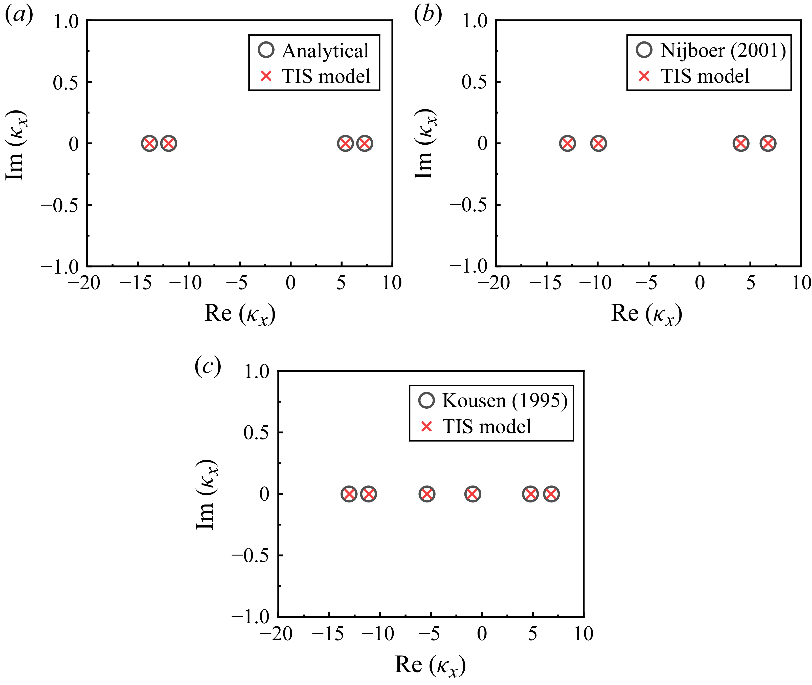
Axial wavenumbers through the TIS model and existing results under the hard-walled boundary condition. (a) Uniform axial flow,
 $m=-2, r_h/r_t=0.4, \omega /\bar {c}=10, \bar {M}_x=0.3$
; (b)
 $\bar {\bar {\varOmega }}_v=0.2$
,
 $m=-2, r_h/r_t=0.4, \omega /\bar {c}=10, \bar {M}_x=0.3$
(Nijboer Reference Nijboer2001); (c)
 $\bar {\bar {\varOmega }}_s=0.3$
,
 $m=-2, r_h/r_t=0.25, \omega /\bar {c}=10, \bar {M}_x=0.3$
(Kousen Reference Kousen1995).

3.1. Acoustic propagation with radially dependent swirling flows
To assess the accuracy of the TIS model in calculating the axial wavenumber influenced by the different kinds of mean flow, we compare its results for uniform axial mean flow, free vortex swirl and solid vortex swirl under hard-walled boundary conditions with theoretical and numerical results in the existing literature. The axial wavenumbers are presented in figure 3, which demonstrates that the TIS model accurately captures the axial wavenumbers for various mean flow conditions, thereby validating its effectiveness.
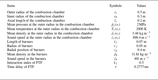
Moreover, in view of the lack of adequate verification of the effects of swirling flows on thermoacoustic instabilities, this study examines the influence of the CCS and ACS on frequencies and growth rates, respectively. To verify the correctness of the TIS model developed in § 2 and also to analyse the effect of swirling flows on thermoacoustic instability, the combustion chamber shown in figure 1 is considered. The mean flow quantities and geometrical parameters are provided in table 1, while additional parameters not listed in table 1 can be derived from conservation relationships at the interface between the burners and the combustion chamber (
 $x_b{-}x_b$
interface). These parameters remain constant unless otherwise stated. It should be noted that the parameters presented in table 1 are referenced against a typical annular combustion chamber of aero engines, which is characterized by a circumferential length significantly greater than its axial length. This configuration results in the first-order azimuthal mode being the least-order mode within the combustion chamber. According to eigenvalue theory of dynamic systems (Chandrasekhar Reference Chandrasekhar1961; Bhatia & Szegö Reference Bhatia and Szegö2002), the least-order mode is particularly susceptible to thermoacoustic instabilities. Therefore, the effect of swirling flows on thermoacoustic instability of the first-order azimuthal mode will be validated and analysed in the following sections.
Geometrical and gas values of the model combustor.

3.2. Complex eigenfrequencies with the uniform circumferential mean flow
The TIS model is reduced to consider only the circumferential mean velocity
 $\bar {M}_{\theta }$
, while the axial mean velocity is neglected (
 $\bar {M}_x=0$
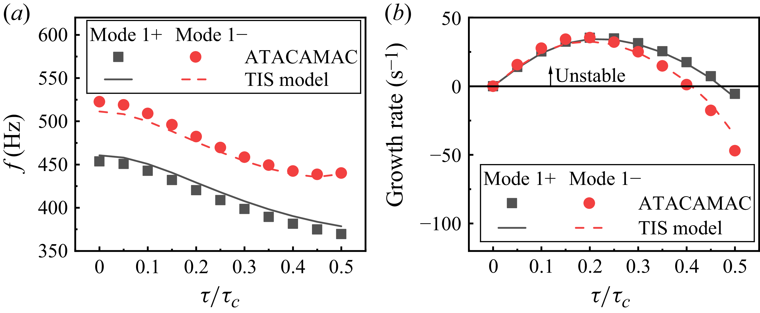
) in order to facilitate comparison with the existing theoretical work (Bauerheim et al. Reference Bauerheim, Cazalens and Poinsot2015) and validate the TIS model. The frequencies and growth rates of the first-order azimuthal mode obtained by these methods are presented in figure 4, with
 $\tau _c$
representing the time period of the first-order azimuthal mode. It should be noted that the two branches of the first-order azimuthal modes are degenerate under symmetrical conditions, i.e. the azimuthal mode
 $m=1$
(denoted as mode
 $1+$
) and azimuthal mode
 $m=-1$
(denoted as mode
 $1-$
) have the same frequencies and growth rates. However, as illustrated in figure 4, the introduction of swirling flows leads to flow symmetry breaking, which leads to the occurrence of the non-degenerate azimuthal modes. This symmetry breaking leads to frequency splitting; specifically, the non-degenerate azimuthal modes feature different frequencies and growth rates. In comparison with existing methods, the TIS model can accurately capture the influence of circumferential mean flow on the frequencies and growth rates of mode
 $1+$
and mode
 $1-$
, thereby validating its capability in addressing thermoacoustic instability.
Frequencies and growth rates of the first-order azimuthal modes with the effect of circumferential mean flow: (a) frequencies; (b) growth rates. The derivation of the ATACAMAC method is detailed in Bauerheim et al. (Reference Bauerheim, Cazalens and Poinsot2015).

3.3. Complex eigenfrequencies with the uniform axial mean flow
Similarly, in the reduced case of the TIS model, i.e. with only axial mean flow while neglecting the circumferential mean velocity in the combustion chamber, the correctness of TIS model in calculating the axial mean flow on thermoacoustic instability is validated by reducing the TIS model to include only ACS, when compared with the existing ‘network method’ (Akamatsu & Dowling Reference Akamatsu and Dowling2001; Zhang et al. Reference Zhang, Wang, Li and Sun2020). Wherein, the axial mean velocity in the combustion chamber is obtained by satisfying the conservation matching condition for the mean quantities at the
 $x_b{-}x_b$
interface, which can be mathematically expressed as
 \begin{equation} \bar {M}_x=\frac {\bar {\rho }_b \bar {M}_b \bar {c}_b N_f S_f}{\bar {\rho }_c \bar {c}_c S_c}. \end{equation}
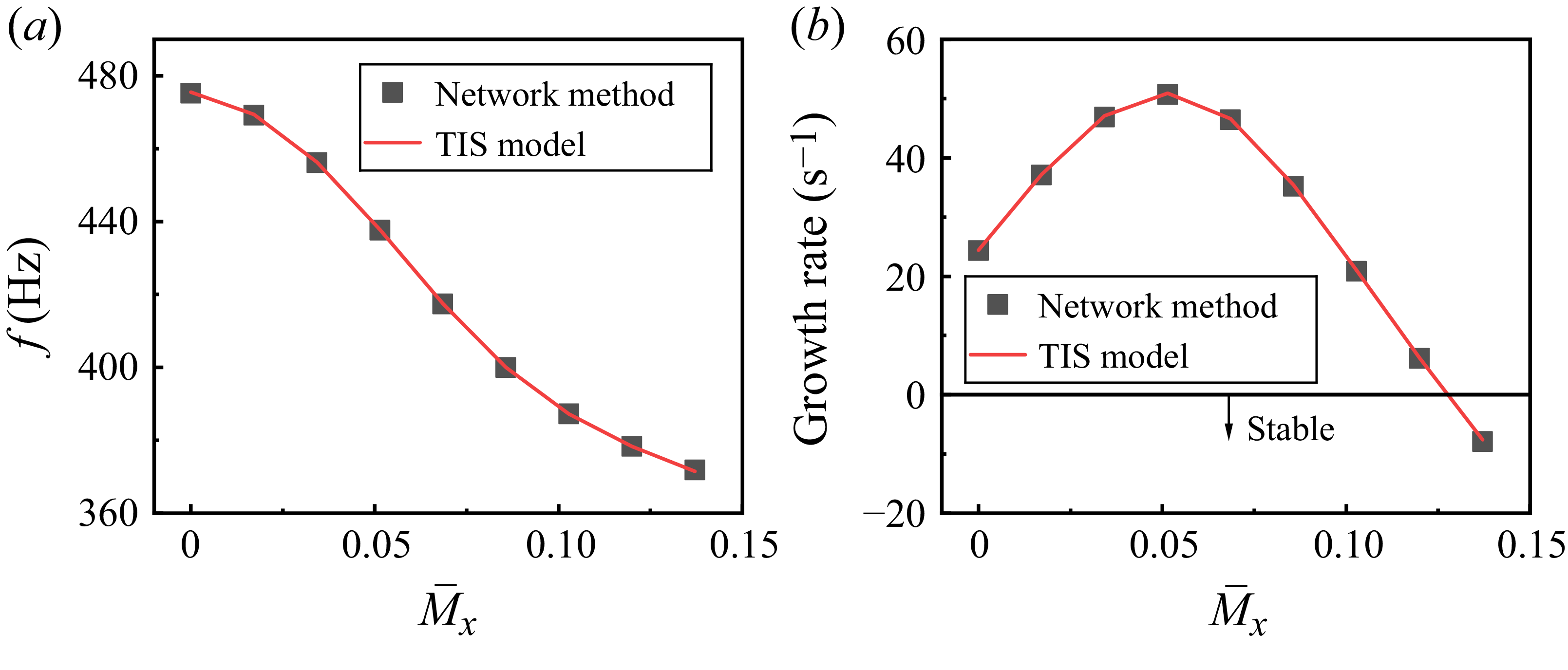
As shown in figure 5, the frequencies and growth rates of the first-order azimuthal mode are shown to be consistent, thus confirming the correctness of the TIS model with the axial mean flow.
Frequencies and growth rates of the first-order azimuthal modes with the effect of the axial mean flow: (a) frequencies; (b) growth rates. The derivation of the ‘network method’ is detailed in Akamatsu & Dowling (Reference Akamatsu and Dowling2001) and Zhang et al. (Reference Zhang, Wang, Li and Sun2020).

Collectively, these three cases validate the TIS model to accurately calculate the axial wavenumbers under swirling conditions without the effect of flame responses, as well as complex eigenfrequencies influenced by both unsteady heat release rates in the burners and circumferential/axial mean flow. With the TIS model validated, the effects of swirling flows in the combustion chamber on thermoacoustic instabilities are discussed in the following sections.
4. The oscillation frequencies and growth rates with radially independent/dependent flow profiles
The three cases presented in § 3 validate the correctness of the TIS model in calculating the effects of circumferential mean flow and axial mean flow on stability, informed by comparisons with existing results. Specifically, the results depicted in figure 4 show that the presence of circumferential mean flow induces symmetry breaking, transforming the azimuthal modes from degenerate modes to non-degenerate modes. This transition results in pronounced differences in frequencies and growth rates of the non-degenerate modes. In contrast, figure 5 shows that the axial mean flow does not affect the symmetry of azimuthal modes under symmetrical conditions, yielding identical frequencies and growth rates for the degenerate azimuthal modes. Moreover, it is evident that the frequencies and growth rates of the degenerate modes are significantly affected by the axial mean flow. Consequently, the characteristics of thermoacoustic instability under swirling flows, accounting for both circumferential and axial mean flow, will be discussed in the subsequent sections.
4.1. Thermoacoustic instability with radially independent flows
4.1.1. Characteristics of stability maps for non-degenerate modes
To facilitate a comparison of the frequencies and growth rates of mode
 $1+$
and mode
 $1-$
under the influence of only circumferential mean velocity and axial mean velocity presented in § 3, also to simplify the complexity of the analysis by isolating the effects of swirling flows on the frequencies and growth rates, we assume that CCS and ACS are uniform, meaning that
 $\bar {M}_x$
and
 $\bar {M}_{\theta }$
are radially independent. Thus, the mean pressure, mean density, and sound speed are radially independent under swirling flow conditions.
The parameters of the combustors are detailed in table 1. Similar to the validation case parameters, additional quantities necessary for calculations, but not included in table 1, can be derived from matching conditions at the
 $x_b{-}x_b$
interface.
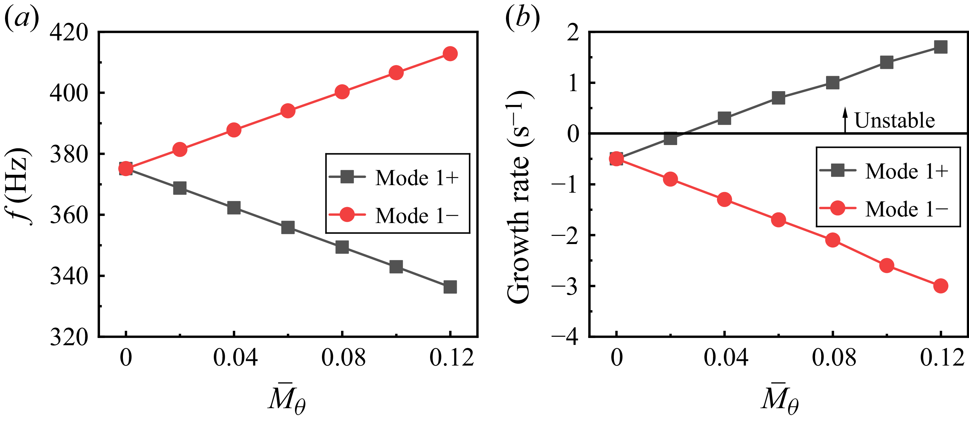
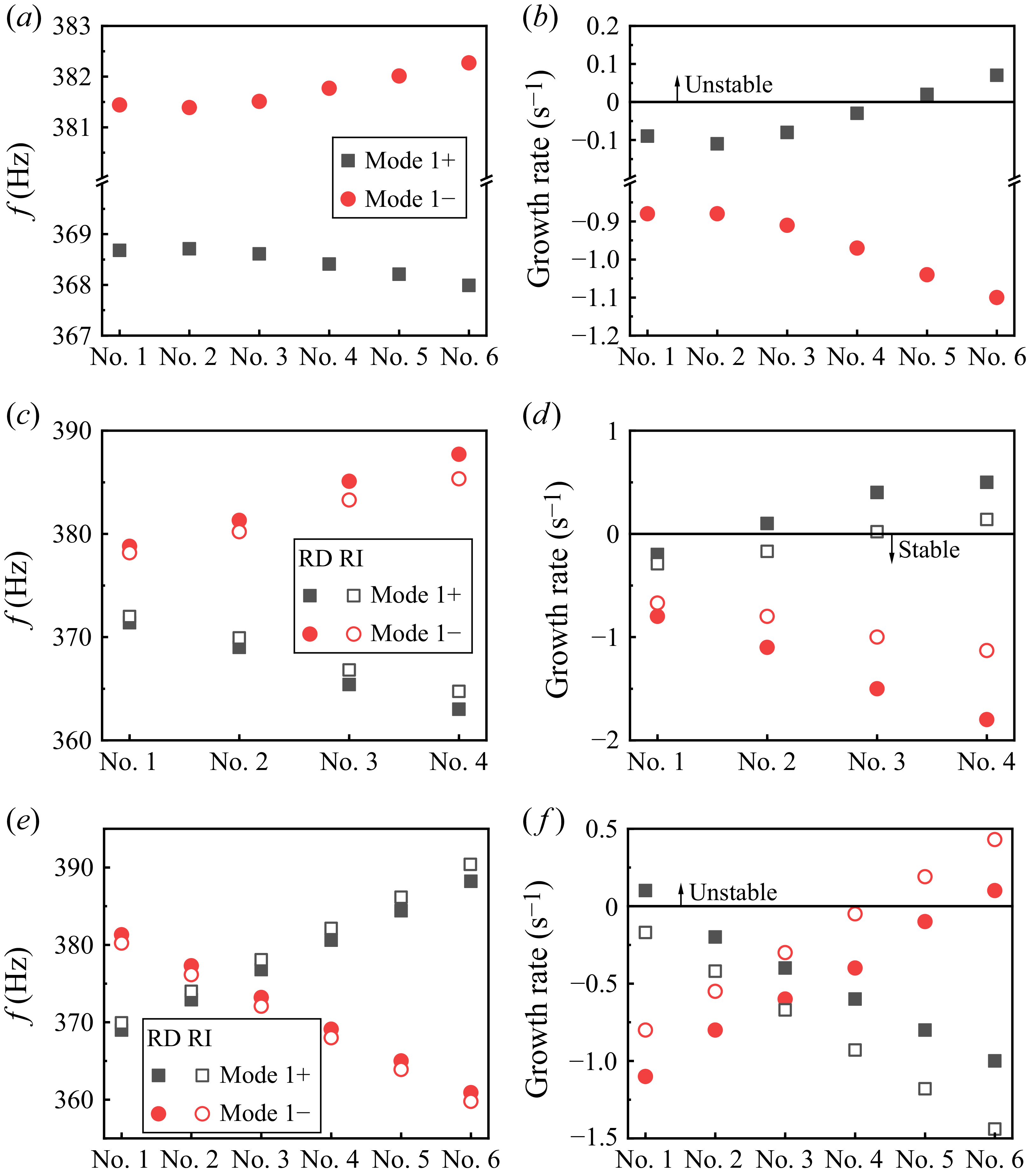
Figure 6 depicts the frequencies and growth rates of the first-order azimuthal non-degenerate modes under the influence of swirling flows. Results show that the ACS shows the same influence tendency on the frequencies and growth rates of mode
 $1+$
and mode
 $1-$
, i.e. the frequency decreases while the growth rate initially rise but subsequently decline with the increase of the ACS. Meanwhile, figure 6 reveals distinctly different trends in the frequencies and growth rates of mode
 $1+$
and mode
 $1-$
as a function of the CCS. An increase in CCS causes more pronounced frequency and growth rate splitting for mode
 $1+$
and mode
 $1-$
.
Frequencies and growth rates versus swirling flows: (a) frequencies of mode
 $1+$
; (b) growth rates of mode
 $1+$
; (c) frequencies of mode
 $1-$
; (d) growth rates of mode
 $1-$
.

The contrasting characteristics of frequencies for modes
 $1+$
and mode
 $1-$
can be attributed to the interaction between acoustic waves and flow dynamics, as shown in figure 7, i.e. the Doppler effect. The mode
 $1+$
represents the acoustic waves rotating clockwise while mode
 $1-$
corresponds to the acoustic waves rotating anticlockwise. When the CCS is positive and directed anticlockwise, it opposes the acoustic propagation of mode
 $1+$
, resulting in significant stretching of the acoustic waves and a corresponding decrease in frequency. In contrast, mode
 $1-$
shows an opposite behaviour: as the CCS increases, the acoustic waves are compressed, leading to a significant increase in frequency. Consequently, the frequencies of mode
 $1+$
are lower than those of mode
 $1-$
. As CCS increases, the Doppler effect intensifies, leading to more significant frequency splitting. When CCS is negative, it has a completely different effect on mode
 $1+$
and mode
 $1-$
in comparison with the condition of positive CCS. Namely, CCS increases the frequency of corotating acoustic waves while decreasing the frequency of counter-rotating acoustic waves.
Sketch of the CCS and acoustic waves: (a) CCS directed anticlockwise; (b) CCS directed clockwise.

Meanwhile, the growth rate for mode
 $1+$
rises with increasing CCS, whereas that of mode
 $1-$
decreases. This divergence in behaviour suggests that, when the magnitudes of the growth rates are small, an increase in CCS leads to contrasting stability behaviours for mode
 $1+$
and mode
 $1-$
. Taking an example with a Mach number
 $\bar {M}_x=0.128$
for ACS, figure 8 illustrates the effects of CCS on the frequencies and growth rates of mode
 $1+$
and mode
 $1-$
. Initially, the first-order azimuthal mode is degenerate when CCS is neglected, resulting in identical frequencies and growth rates for both mode
 $1+$
and mode
 $1-$
. However, once CCS is accounted for, the first-order azimuthal mode becomes non-degenerate, exhibiting distinct frequencies and growth rates for mode
 $1+$
and mode
 $1-$
. This splitting phenomenon is more pronounced with increasing CCS. Notably, the growth rate of mode
 $1+$
increases with CCS, indicating a transition from stability to instability and highlighting the effects of swirling flows on frequency and stability characteristics.
Frequencies and growth rates of the non-degenerate modes versus CCS: (a) frequencies; (b) growth rates.

4.1.2. Stability analysis conducted via acoustic energy assessments
To elucidate the mechanism underlying stability transitions for mode
 $1+$
and mode
 $1-$
in the presence of swirling flows, we analyse acoustic energy across critical interfaces: the combustion chamber inlet (
 $x_b{-}x_b$
interface) and outlet (
 $x_c{-}x_c$
interface). The acoustic energy flux at the combustion chamber inlet quantifies the influence of the unsteady heat release within the burners on thermoacoustic instabilities. Conversely, the acoustic energy flux at the combustion chamber outlet characterizes the acoustic energy leaving the confined space. In an ideal acoustic medium, the time-average acoustic energy
 $E$
is defined as (Morfey Reference Morfey1971; Glegg & Devenport Reference Glegg and Devenport2017)
 \begin{equation} E = \int _S I \boldsymbol{\cdot }\boldsymbol{n}^0 \textrm{d}S, \end{equation}
with
 \begin{equation} I = \langle \tilde {B} \tilde {H}\rangle, \end{equation}
where
 $I$
,
 $\boldsymbol{n}^0$
,
 $\tilde {B}$
and
 $\tilde {H}$
represent the acoustic energy flux, wall normal, perturbations in mass flux per unit area and stagnation enthalpy, respectively. The angle brackets
 $\langle\;\rangle$
represent a time average of the product of the real components of these quantities. In the context of homentropic flow and when considering only first-order perturbations, it yields
 \begin{align} &\tilde {B} = \bar {\rho }_c \boldsymbol{\tilde {u}} + \tilde {\rho }_c \boldsymbol{\bar {u}}, \end{align}
 \begin{align} &\tilde {H} = \tilde {p}_c/\bar {\rho }_c + \boldsymbol{\bar {u}} \boldsymbol{\cdot }\boldsymbol{\tilde {u}}. \end{align}
The time-average acoustic energy transmissions at the combustion chamber inlet (
 $x_b{-}x_b$
interface) and outlet (
 $x_c{-}x_c$
interface) is denoted as
 $E_{x_b}$
and
 $E_{x_c}$
, respectively. Consequently, the total acoustic energy accumulated within the combustion chamber is expressed as
 \begin{equation} E_t = E_{x_b} - E_{x_c}. \end{equation}
A positive net time-average acoustic energy (
 $E_t\gt 0$
) signifies that the influx of acoustic energy at the combustion chamber inlet exceeds the efflux through the outlet, leading to a positive accumulation of acoustic energy within the chamber, which is indicative of thermoacoustic instability. Conversely,
 $E_t\lt 0$
implies that the time-average acoustic energy leaving at the outlet surpasses the acoustic energy influx, corresponding to a stable condition.
We define a normalized acoustic energy with the expression of
 \begin{equation} \bar {\bar {e}} = \frac {E_t}{E_{x_b}} = 1 - \frac {E_{x_c}}{E_{x_b}}. \end{equation}
The normalized acoustic energy
 $\bar {\bar {e}}$
is defined to characterize the thermoacoustic energy within the combustion system, with its value providing a basis for assessing stability behaviour and energy transition mechanisms. Specifically, we have the following.
-
(i) Equilibrium state (
$\bar {\bar {e}} = 0$
). This condition represents an acoustic energy equilibrium where the acoustic energy influx at the combustion chamber inlet equals the acoustic energy efflux through the outlet. This equilibrium corresponds to the critical threshold between stable and unstable thermoacoustic regimes. -
(ii) Stability criteria (
$\bar {\bar {e}} \lt 0$
and
$\bar {\bar {e}} \gt 0$
). A negative value (
$\bar {\bar {e}} \lt 0$
) signifies a stable condition, as the acoustic energy efflux exceeds energy gain. Conversely, a positive value (
$\bar {\bar {e}} \gt 0$
) denotes instability, indicating acoustic energy accumulation due to unsteady heat release exceeding acoustic energy efflux. -
(iii) Non-Dissipative limit (
$\bar {\bar {e}} = 1$
). At this value, acoustic energy dissipation at the combustion chamber outlet is negligible. The thermoacoustic instability of the azimuthal mode is thus predominantly governed by phase-coupled interactions between oscillations of pressure and unsteady heat release in the burners. -
(iv) Parametric sensitivity (
$\bar {\bar {e}} \neq 0$
,
$\bar {\bar {e}} \neq 1$
). The parameter
$\bar {\bar {e}}$
quantifies the relative influence of a given variable on energy transmission. When
$E_{x_b}\gt 0$
, a decrease in
$\bar {\bar {e}}$
corresponds to an increase in the ratio
$E_{x_c}/E_{x_b}$
. This trend implies that the parameter exerts a stronger influence on energy transmission at the outlet relative to energy generation at the inlet. Conversely, an increase in
$\bar {\bar {e}}$
highlights the dominant effect on modulating energy generation in the burners at the combustion chamber inlet over energy transmission at the outlet.


The normalized acoustic energy
 $\bar {\bar {e}}$
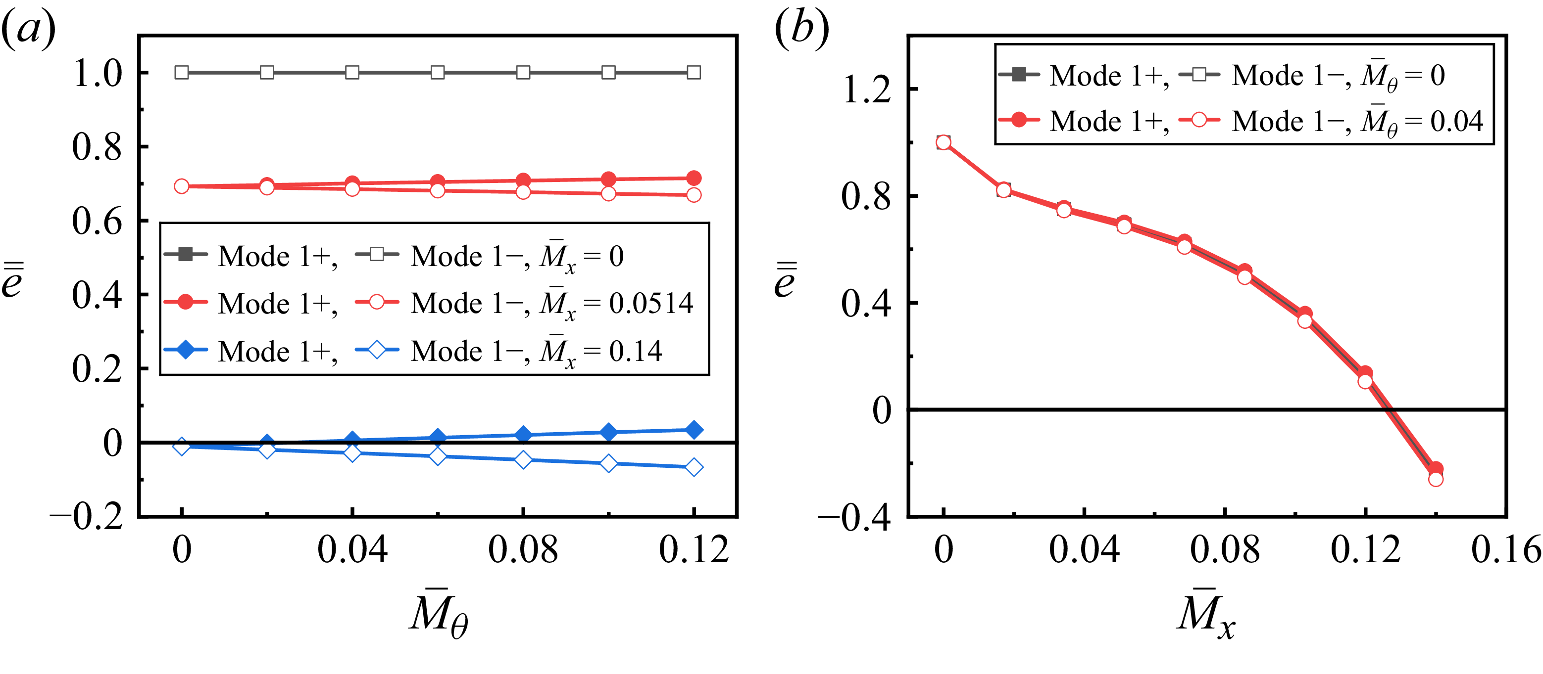
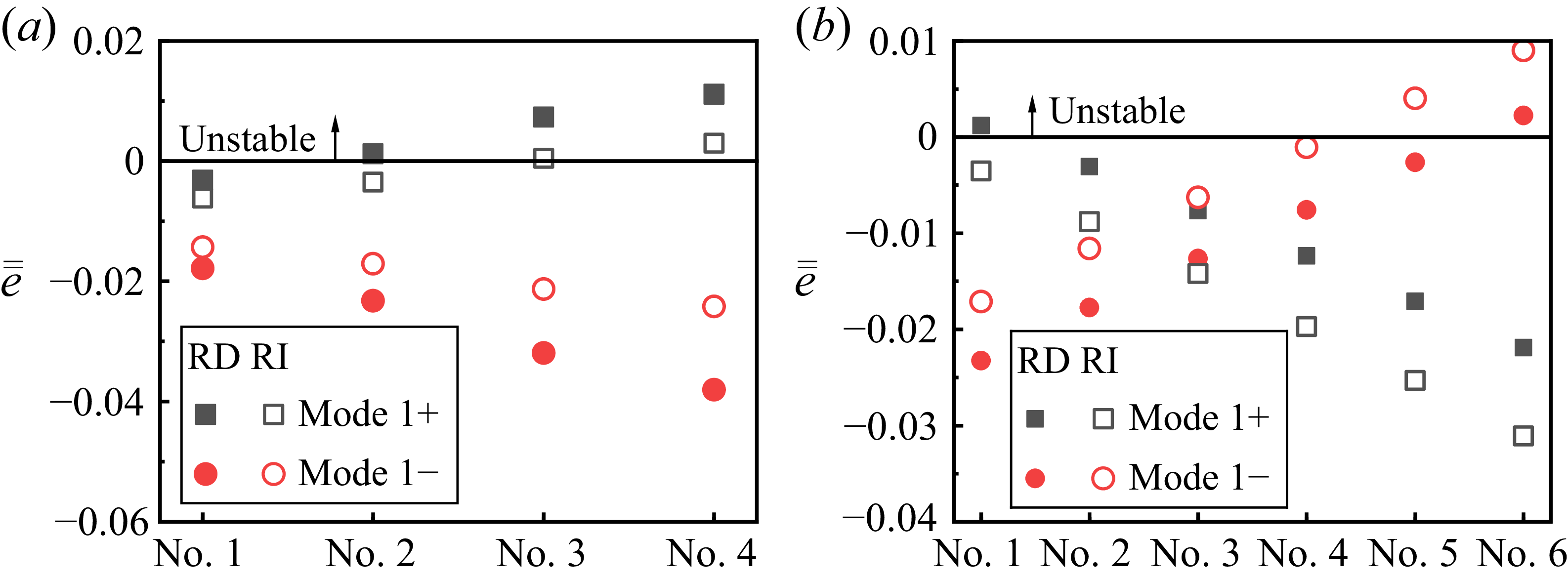
obtained through (4.1)–(4.5), is plotted as a function of CCS and ACS in figure 9. The data presented in figure 9 correspond to the flow configurations analysed in figures 6(b) and 6(d), which represent specific CCS and ACS conditions, respectively.
Normalized acoustic energy
 $\bar {\bar {e}}$
versus CCS and ACS: (a)
 $\bar {\bar {e}}$
versus CCS; (b)
 $\bar {\bar {e}}$
versus ACS.

Figure 9(a) shows that at a zero axial Mach number (
 $\bar {M}_x = 0$
), the normalized acoustic energy attains a baseline value of
 $\bar {\bar {e}} = 1$
. This implies the absence of acoustic energy transmission at the combustion chamber outlet under static axial flow conditions, signifying that the growth rates of mode
 $1+$
and mode
 $1-$
arise exclusively from acoustic energy generated through the coupling between flame responses and acoustic pressure. Incremental increases in
 $\bar {M}_x$
(
 $\bar {M}_x = 0.0514$
and
 $\bar {M}_x = 0.14$
) reveal distinct trends in
 $\bar {\bar {e}}$
of mode
 $1+$
and mode
 $1-$
. First, both modes exhibit slight yet inversely correlated sensitivity to the variations of CCS. For mode
 $1+$
,
 $\bar {\bar {e}}$
increases monotonically with
 $\bar {M}_{\theta }$
, implying that the variations of CCS have a more pronounced effect on the acoustic energy generated by the unsteady heat release, whereas mode
 $1-$
exhibits a contrasting dependence. In other words, in comparison with the variations in acoustic energy gain resulting from unsteady heat release at the combustion chamber inlet, an increase in CCS leads to a reduction in acoustic energy transmission of counter-propagating acoustic waves at the outlet boundary while enhancing that of copropagating acoustic waves. Second, the divergence of
 $\bar {\bar {e}}$
between the mode
 $1+$
and mode
 $1-$
amplifies with concurrent increases in
 $\bar {M}_x$
and
 $\bar {M}_{\theta }$
, a trend consistent with the growth rate behaviour in figure 6. These findings underscore the interdependence of ACS and CCS in modulating acoustic energy and thermoacoustic instability.
Figure 9(b) illustrates the relationship between
 $\bar {\bar {e}}$
and ACS. Notably,
 $\bar {\bar {e}}$
decreases significantly with increasing
 $\bar {M}_x$
across all tested CCS. This attenuation reflects a progressive dominance of outlet boundary effects over unsteady heat release as ACS accelerates. Specifically, increased ACS enhance acoustic energy transmission through the combustion chamber outlet, thereby affecting the stability of the azimuthal modes. Furthermore, parametric comparisons reveal that ACS exerts a more pronounced influence than CCS on acoustic energy. This comparative analysis suggests that axial momentum, oriented perpendicular to the cross-sections of the chamber inlet/outlet, facilitates greater acoustic energy flux across boundaries relative to contributions from tangential momentum.
Moreover, results demonstrate that CCS significantly modulates thermoacoustic stability transitions primarily near marginal stability thresholds (where the growth rate approaches zero), in the context of the FTF with axial velocity perturbations. Meanwhile, investigations indicate that incorporating circumferential velocity perturbations into FTF has a negligible impact on frequencies and growth rates but significantly modifies spinning ratios (Li et al. Reference Li, Yang, Li and Zhu2019). This limited sensitivity presented in prior findings is attributed to the circumferential velocity perturbations on the FTF (indicated by the interaction index) generally much smaller than the axial velocity perturbations (Li et al. Reference Li, Yang, Li and Zhu2019). The present results additionally demonstrate that in the absence of ACS, acoustic energy transmission at the combustion chamber outlet diminishes to negligible levels, resulting in minimal effects on the stability under minor changes in flame response. Collectively, these findings underscore the critical role of outlet boundary conditions in affecting thermoacoustic instability within swirling flow configurations.
4.2. Thermoacoustic instability with radially dependent flows
The effect of swirling flows on the thermoacoustic instability in the case of a uniform flow field (i.e. ACS and CCS are radially independent) is examined in § 4.1. However, in practical combustion chambers, the mean flow field is often non-uniform, which may alter the characteristics of thermoacoustic instability. Given that the TIS model developed in § 2 incorporates the effect of radially dependent flow field, this subsection focuses on evaluating the effect of typically radially dependent axial mean flows and swirling flows on thermoacoustic instabilities.
4.2.1. Radially dependent axial mean flows
It should be noted that the radially dependent axial mean velocity does not introduce an additional force term as shown in § 2.1. Therefore, the mean pressure, mean density and sound speed are still considered to be radially independent, i.e. only the axial mean velocity is radially dependent in this section.
To systematically investigate this effect, three representative cases of radially dependent axial mean velocity are analysed. These cases assume that the CCS is equal to zero (
 $\bar {M}_{\theta }=0$
) to avoid the effect of CCS. The radial distribution patterns of ACS are detailed in table 2 and illustrated in figure 10, with the radial position of the burners fixed at
 $r_p=0.4$
m. These cases share a common feature: the ACS is notably higher at the midradius position. Such a distribution arises from the geometric constraints imposed by burners, which concentrate flow discharge near the chamber’s midradius region, thereby amplifying local axial mean velocities.
Radially dependent axial mean velocity of swirling flows.

Distribution of radially dependent ACS. Here
 $\bar {\bar {M}}_x$
represents the normalized ACS.

Frequencies and growth rates of the degenerate modes versus axial mean velocity: (a) frequencies; (b) growth rates. Case 0 represents the radially independent ACS configuration.

Figure 11 illustrates the frequencies and growth rates of the first-order azimuthal mode under the three profiles of radially dependent ACS. The distribution of ACS in the combustion chamber is determined through conservation conditions at the
 $x_b{-}x_b$
interface. To account for the radially dependent mean ACS within the combustion chamber, the axial mean velocity in the burners is used as a reference, ensuring that the mass flow rate in the combustion chamber remains consistent across all three cases. This allows for a meaningful comparison of the effects of radially dependent ACS on thermoacoustic instability while maintaining the same mass flow rate.
It is observed that both frequency and growth rate exhibit similar trends with increasing ACS. However, the crucial distinction lies in the fact that the radially dependent ACS results in differences in the magnitudes of frequency and growth rate. For example, in Case 3, the radially dependent ACS results in contrasting stability behaviours for the first-order azimuthal mode at the condition of
 $\bar {M}_b=0.4$
in comparison with other cases.
Sketch of radially dependent CCS.

4.2.2. Radially dependent swirling flows
In practical scenarios where the swirling flows produced by the burners is uniform – such as a purely anticlockwise rotation – this makes CCS radially dependent. Specifically, the CCS direction is anticlockwise at the outer radius and clockwise at the inner radius, as shown in figure 12. This necessitates a further investigation into the effects of radially dependent mean flows on thermoacoustic instability, which is discussed below.
To model the non-uniformity of swirling flows, we consider a combination of solid body swirl and free vortex swirl, as described by (2.7c). Three representative cases of radially dependent CCS are examined to characterize this non-uniformity, as illustrated in figure 13. The corresponding strengths of these swirling flow configurations are detailed in table 3. The ACS is
 $\bar {M}_x=0.128$
for these cases. In addition, it should be noted that the inclusion of the swirling flows leads to the existence of centrifugal forces, thus making the mean pressure, mean density, and sound speed radially dependent. The radial non-uniform distribution of these mean quantities can be obtained from (2.7)–(2.9).
For case 1, six swirling flow configurations (labelled as Nos. 1–6) are constructed by varying the strengths of both free vortex swirl and solid body swirl. These configurations possess distinct radially dependent CCS profiles but share a constant radially integrated value, as illustrated in figure 13(a). Wherein, configuration No. 1 represents a radially independent baseline (
 $\bar {M}_{\theta }=0.02$
). These configurations aim to isolate the effect of the radially dependent CCS profiles on thermoacoustic instabilities, independent of the overall circumferential mean velocities.
In contrast to Case 1, the CCS profiles in each of the other two cases feature similar radial distributions but different radially integrated circumferential mean velocities.
For Case 2, four swirling flow configurations (labelled as Nos. 1–4) are analysed by varying the strengths of both free vortex swirl and solid body swirl. Notably, the mean circumferential Mach number (
 $\bar {M}_{\theta }$
) for these configurations is zero at a specified radial location
 $r_{sl}$
, as shown in figure 13(b). This phenomenon corresponds to the configuration of the counteracting swirl directions at the outer and inner radii, which cancel out to produce zero CCS at the fixed position of
 $r_{sl}$
. Moreover, the direction of the CCS is opposite on either side of this fixed point
 $r_{sl}$
, with its magnitude increasing towards the wall.
The strengths of solid body swirl and free vortex swirl for radially dependent CCS.

Distributions of radially dependent CCS: (a) Case 1; (b) Case 2; (c) Case 3.

For Case 3, six swirling flow configurations (labelled as Nos.1–6) are investigated by modifying the strength of the free vortex swirl while maintaining a constant strength for the solid body swirl. This approach allows for an analysis of how variations in free vortex swirl strength influence the frequencies and growth rates of thermoacoustic instability. As shown in figure 13(c), the CCS transitions from predominantly anticlockwise in No. 1 to predominantly clockwise in No. 6.
Frequencies and growth rates with the effect of radially dependent CCS: (a) frequencies of Case 1; (b) growth rates of Case 1; (c) frequencies of Case 2; (d) growth rates of Case 2; (e) frequencies of Case 3; (f) growth rates of Case 3. Solid and hollow symbols denote the results for radially dependent (RD) CCS profiles and their corresponding radially independent (RI) averaged profiles, respectively.

Figure 14 illustrates the influence of radially dependent CCS profiles on the frequency and stability characteristics of mode
 $1+$
and mode
 $1-$
. The results for these modes are denoted by solid symbols and are labelled as RD for both Case 2 and Case 3 in the subpanels. As shown in figure 13(a), the radial separation of CCS intensifies progressively from No. 1 to No. 6. This increasing non-uniformity correlates with a corresponding divergence in the frequencies and growth rates of mode
 $1+$
and mode
 $1-$
, as observed in figures 14(a) and 14(b). Consequently, a stability shift occurs for mode
 $1+$
when its growth rate approaches zero. This implies that, even with a constant radial integral of the CCS, different radially dependent distributions can lead to divergence in the frequencies and growth rates for both mode
 $1+$
and mode
 $1-$
. Furthermore, it is expected that this divergence will be amplified by higher circumferential mean velocities.
A similar trend is observed for Case 2 (figures 14
c and 14
d), where increased radial non-uniformity in the CCS leads to a greater separation in the frequencies and growth rates between mode
 $1+$
and mode
 $1-$
. Specifically, figure 14(d) reveals that mode
 $1+$
exhibits a negative growth rate (stable) in No. 1, whereas it transitions to positive growth rates (unstable) in Nos. 2–4. These findings collectively suggest that enhanced radial non-uniformity in the CCS destabilizes mode
 $1+$
.
Figures 14(e) and 14(f) further demonstrate that shifting the dominant CCS direction from anticlockwise (i.e.
 $\bar {M}_{\theta }\gt 0$
) in No. 1 to clockwise (
 $\bar {M}_{\theta }\lt 0$
) in No. 6 induces distinct trends: the frequency of mode
 $1+$
increases gradually, while its growth rate decreases. Conversely, mode
 $1-$
exhibits an inverse response, with frequency decreasing and growth rate increasing. Consequently, mode
 $1+$
remains unstable in No. 1 but stabilizes in Nos. 2–6, whereas mode
 $1-$
transitions from stable (Nos. 1–5) to unstable (No. 6). This behaviour highlights the sensitivity of thermoacoustic stability to radial velocity gradients, particularly at marginal growth rates.
Furthermore, a comparative analysis of radially dependent and radially independent CCS profiles on frequencies and growth rates is presented in figures 14(c) to 14(f). To ensure a constant basis for comparison, the hollow symbols denote the results for radially independent CCS profiles whose radial integral is equivalent to that of the corresponding radially dependent profiles. Results show that frequencies and growth rates for weakly radially dependent CCS profiles closely align with those of the radially independent baseline. However, as the radial non-uniformity intensifies, a progressive deviation from this baseline is observed (figures 14 c and 14 d). This trend demonstrates a consistent physical mechanism with figures 14(a) and 14(b), confirming that the degree of radial non-uniformity directly affects the divergence in frequencies and growth rates. Given the consistent degree of radial non-uniformity in the CCS profiles from No. 1 to No. 6 in Case 3 (figure 13 c), the divergence in frequency and growth rate between the radially dependent and radially independent conditions remains approximately constant across all configurations (figures 14 e and 14 f).
The normalized acoustic energy
 $\bar {\bar {e}}$
in figures 15(a) and 15(b) exhibits congruent trends with the growth rates depicted in figures 14(d) and 14(f), respectively. This correlation confirms that the radially dependent CCS affects the acoustic energy exchange at the combustion chamber inlet and outlet, which critically dictates the growth rates and stability behaviours. Specifically, in comparison with the acoustic energy generation originating from the burner region, the radially integrated positive CCS predominantly amplifies acoustic energy transmission at the outlet boundary for mode
 $1-$
, while exhibiting an opposite trend for mode
 $1+$
. These asymmetries highlight the distinct mechanisms by which radially dependent CCS influence thermoacoustic instability: outlet boundary-dominated energy transfer for mode
 $1-$
versus flame-dominated energy production for mode
 $1+$
under radially integrated positive CCS configuration. Moreover, compared with the radially independent baseline, the radially dependent CCS profile influences acoustic energy transmission at the boundary conditions.
Normalized acoustic energy
 $\bar {\bar {e}}$
versus radially dependent CCS: (a) Case 2; (b) Case 3.

In addition, the frequency variations in figures 14(a), 14(c) and 14(e) align with the schematic in figure 8. For No. 1 to No. 6 in figure 14(a), the net CCS is dominated by anticlockwise rotation (
 $\bar {M}_{\theta }\gt 0$
). Mode
 $1+$
propagates opposite to this dominant flow, subjecting the acoustic wave to an adverse flow that reduces its frequency from No. 1 to No. 6. In contrast, mode
 $1-$
aligns with the flow direction, undergoing constructive compression and an increase for frequency. Similarly, the radially dependent CCS profiles in figures 13(b) and 13(c) explain the frequency trends in figures 14(c) and 14(e) through analogous mechanisms, respectively.
It is important to note that these findings pertain to annular combustion chambers with relatively large hub ratios. In chambers with smaller hub ratios – such as can-type combustion chambers in industrial gas turbines and afterburners in aero engines – it is anticipated that the influence of radially dependent CCS on modal characteristics would be even more pronounced.
4.3. Further discussion on the effectiveness and limitations of the TIS model
Modern gas turbine combustion chambers are characterized by highly complex turbulent flows, which involve vortex breakdown and multiphase flow, attracting growing research interest in their impact on combustion dynamics. The theoretical framework and numerical analysis presented in this work attempt to uncover the physical mechanism of thermoacoustic instability by focusing on the interactions among acoustic perturbations, mean swirling flows, and flame responses in the confined spaces. The relevant characteristic equation is described by (2.36), referred to as the TIS model. It is noted that whether this model is simplified to align with prior network-based thermoacoustic approaches or acoustic propagation problems, a good agreement is observed in the comparisons shown in figures 3 to 5. However, it remains uncertain whether the prior network-based thermoacoustic approaches can fully reveal the swirling mechanism without incorporating radially dependent parameters, particularly in combustors with larger hub ratios. In fact, whenever a mean swirling flow is present, all mean parameters demonstrate radial dependence according to conservation laws, regardless of the combustion hub ratio. The assumption of radially independent uniform flows is merely a special case within various possible radial distributions. This raises an open question regarding how such non-uniform flow distributions affect thermoacoustic instability. Therefore, elucidating this question constitutes the central objective of the present investigation.
This work addresses the effects of radially dependent velocities on thermoacoustic instabilities, based upon the TIS model, as shown in figures 11 and 14. Meanwhile, the TIS model is also capable of evaluating the effects of other radially dependent mean quantities such as pressure, density, vorticity intensity and sound speed – as derived from conservation laws. Model parameters are selected based on a typical aero-engine annular combustion chamber, with appropriate modifications to serve two purposes: validating the TIS model against existing results and analysing the influence of swirling flows for practical applications. Results indicate that even in annular chambers with high hub ratios, radially dependent velocity distributions alter frequencies and growth rates. Although the effect of radial non-uniformity is less pronounced than that of the CCS, it can trigger stability transitions at marginal growth rates. This suggests that radial non-uniformity exerts a more significant effect in systems with smaller hub ratios, such as industrial can-type combustors and aero-engine afterburners, indicating the broader applicability and effectiveness of the TIS model for practical scenarios.
On the other hand, as introduced in § 2.4, the outlet boundary condition is an important component for constituting the characteristic equation within the finite domain. The expression given in (2.35) directly affects the standing-wave solution in the axial direction. Moreover, the combustor features complex outlet boundary conditions associated the with three-dimensional wave reflections caused by the guide vanes of the turbine and flow fields. It is anticipated that the real outlet boundary condition is substantially more intricate than that described in (2.35), naturally showing the limitations of the TIS model in analysing complex boundary conditions in its current form.
Future work can extend the established TIS model to incorporate additional parameters for a more accurate representation of real-world phenomena. First, the flame responses affected by localized swirl structures can be integrated by replacing (2.26) without significant analytical difficulty, providing a more realistic basis for instability analysis. Furthermore, while the momentum matching condition in (2.29) is applied at the central position, imposing it across the entire burner–chamber interface would enable the analysis of distributed flame responses without substantially increasing model complexity. Second, regarding the complex outlet boundary condition of the combustion chamber, extending (2.35) to account for different outlet impedances would facilitate the analysis of these boundary effects on thermoacoustic instability. These proposed developments would align the model more closely with real-world physics while avoiding significant theoretical challenges, thereby enabling a more accurate analysis of key factors in practical applications.
5. Conclusions
This study investigates the influence of intensifying swirling flows within confined combustion chambers on thermoacoustic instability through the development of a three-dimensional thermoacoustic instability under the swirling flow (TIS) model. The TIS model, grounded in linearized Euler equations, enables the prediction of thermoacoustic instabilities under combined axial and circumferential flow conditions. The governing equations for mean flow parameters and perturbations in a three-dimensional annular combustion chamber are formulated, explicitly incorporating centrifugal forces induced by swirling flows. This theoretical framework facilitates the derivation of radially dependent mean quantities and the perturbation equations governing instability dynamics. A dispersion relation formulation, comprising ordinary differential equations, is established by integrating conservation matching conditions at the chamber inlet (linked to unsteady heat release rates) and outlet boundary conditions under swirling flow configurations. Spectral methods are employed to solve this dispersion relation, yielding complex eigenfrequency (frequency and growth rate). The validity of the TIS model is confirmed through three comparative validation cases.
Results reveal that swirling flows disrupt flow symmetry, inducing distinct frequency and growth rate bifurcations in azimuthal mode branches. Enhanced circumferential flow components amplify this bifurcation, whereas axial components modulate both branches with parallel trends. Radially dependent axial and circumferential flow profiles are shown to significantly alter instability characteristics, with the frequency and stability of mode branches correlating with radial integration of circumferential flow gradients. Notably, at low growth rates, increases in axial and circumferential flows trigger stability transitions (stable or unstable) in the first-order azimuthal modes.
The analysis of acoustic energy reveals that, in the absence of axial mean velocity, there is no acoustic energy transmission at the outlet of the combustion chamber when subjected to a node of axial velocity perturbation. In this scenario, the thermoacoustic instability of azimuthal modes is primarily governed by the unsteady heat release within the burners. As the axial mean velocity increases, enhanced acoustic energy transmission through the outlet boundary is observed, which aids in suppressing thermoacoustic instability. In addition, elevated circumferential flows amplify the separation of non-degenerate azimuthal modes, a phenomenon that intensifies with concurrent increases in axial mean velocity. These findings highlight the interdependence of ACS and CCS in influencing acoustic energy and thermoacoustic instability.
The TIS model establishes a foundation for investigating the role of radially dependent parameters (e.g. pressure gradients) in thermoacoustic instability. Systematic investigation of these mechanisms can deepen the understanding of instability complexity in swirling flow environments, offering insights for combustion chamber design and instability mitigation strategies.
Funding
This work was supported by the National Natural Science Foundation of China (nos. 52406037, 52325602 and U2441279) and the China Postdoctoral Science Foundation (nos. GZB20240930 and 2025M774244).
Declaration of interests
The authors report no conflict of interest.