Thermocapillary flows on heated substrates with sinusoidal topography

Jaehyun Yoo; Jaewook Nam; Kyung Hyun Ahn

doi:10.1017/jfm.2018.812

Thermocapillary flows on heated substrates with sinusoidal topography

Published online by Cambridge University Press: 27 November 2018

and

Jaehyun Yoo: Affiliation:
School of Chemical and Biological Engineering, Institute of Chemical Processes, Seoul National University, 1 Gwanak-ro, Gwanak-gu, Seoul 08826, Korea
Jaewook Nam*: Affiliation:
School of Chemical and Biological Engineering, Institute of Chemical Processes, Seoul National University, 1 Gwanak-ro, Gwanak-gu, Seoul 08826, Korea
Kyung Hyun Ahn: Affiliation:
School of Chemical and Biological Engineering, Institute of Chemical Processes, Seoul National University, 1 Gwanak-ro, Gwanak-gu, Seoul 08826, Korea
*: †Email address for correspondence: jaewooknam@snu.ac.kr

Article contents

Abstract
Introduction
Mathematical descriptions
Asymptotic solutions
Numerical validation
Final remarks
References

Rights & Permissions

Abstract

Two-dimensional steady thermocapillary flows in a liquid layer over a substrate, which has a uniform temperature and sinusoidal topography, are investigated by asymptotic theory. Here, the buoyancy effect is negligible and the interface is not significantly disturbed under low Marangoni number and low capillary number. A temperature gradient along the gas/liquid interface causes recirculating flows. For a small aspect ratio, which yields a sinusoidal topography with a long wavelength relative to the mean depth of the liquid layer, the second-order solutions are obtained analytically. The basic solutions show vertical diffusion of heat and vorticity from the substrate and interface, respectively. In the second corrections, the horizontal diffusion of heat weakens the overall flow and the convection of heat intensifies it.

JFM classification

Interfacial Flows (free surface): Capillary flows Convection: Marangoni convection

Information

Type: JFM Papers
Information: Journal of Fluid Mechanics , Volume 859 , 25 January 2019, pp. 992 - 1021
DOI: https://doi.org/10.1017/jfm.2018.812 [Opens in a new window]
Copyright: © 2018 Cambridge University Press

1 Introduction

An interaction between two different fluid molecules across an interface causes a surface tension. Since the surface tension is a state function, it depends on the temperature, composition, electric charge density, etc. of the fluids (Scriven Reference Scriven1960). Therefore, a temperature gradient along the interface invokes a surface-tension gradient, which makes static equilibrium impossible. These phenomena are called thermocapillary flows or thermal Marangoni flows.

Such flows are observed in several systems, including combustion processes (Sirignano & Glassman Reference Sirignano and Glassman1970; Torrance Reference Torrance1971), welding pools (Russo, Akau & Jellison Reference Russo, Akau and Jellison1990; Mills et al. Reference Mills, Keene, Brooks and Shirali1998), crystal-growth processes (Schwabe & Scharmann Reference Schwabe and Scharmann1981; Cuvelier & Driessen Reference Cuvelier and Driessen1986), droplet coalescence and formation (Gupta et al. Reference Gupta, Sbragaglia, Belardinelli and Sugiyama2016; Geri et al. Reference Geri, Keshavarz, Mckinley and Bush2017), etc.

In this study, we focus on thermocapillary flows in liquid layers on heated substrates, which can be encountered in liquid film coatings (Weinstein & Palmer Reference Weinstein, Palmer, Kistler and Schweizer1997). Usually, a flat substrate has been considered for exploring thermocapillary flows under a liquid layer (Birikh Reference Birikh1966; Münch Reference Münch2002; Evans & Münch Reference Evans and Münch2006). Thermal instabilities such as Bénard convection were observed (Eckert, Bestehorn & Thess Reference Eckert, Bestehorn and Thess1998; Tomita & Abe Reference Tomita and Abe2000; Schatz & Neitzel Reference Schatz and Neitzel2001). Recently, however, non-flat or patterned substrates have been employed in liquid film coatings. In wearable electronics, single fibres with electronic functions are converted into fabric structures to achieve flexibility or transparency (Zeng et al. Reference Zeng, Shu, Li, Chen, Wang and Tao2014). Coating, levelling and drying processes are conducted over those substrates with patterns. Such electronics are used to monitor the physical activity and health status in the applications of outdoor clothing or medical devices. Owing to these practical interests, several experimental and numerical studies were carried out for geometrically-patterned substrates (Ismagilov et al. Reference Ismagilov, Rosmarin, Gracias, Stroock and Whitesides2001; Alexeev, Gambaryan-Roisman & Stephan Reference Alexeev, Gambaryan-Roisman and Stephan2005; Fath et al. Reference Fath, Horn, Gambaryan-Roisman, Stephan and Bothe2015). A lubrication-theory-based model is typically used for describing hydrodynamics and energy transport to determine the evolution of the multicomponent thin films (Saprykin et al. Reference Saprykin, Trevelyan, Koopmans and Kalliadasis2007; Frumkin & Oron Reference Frumkin and Oron2016; Pham, Cheng & Kumar Reference Pham, Cheng and Kumar2017).

The asymptotic theory has been successfully used to analytically study numerous types of convection due to buoyancy or thermocapillary force. Cormack, Leal & Imberger (Reference Cormack, Leal and Imberger1974) considered buoyancy-driven flows in a rectangular container bounded by differently heated lateral walls and Poulikakos & Bejan (Reference Poulikakos and Bejan1983) treated flows in an attic space heated from below. Sen & Davis (Reference Sen and Davis1982) and Strani, Piva & Graziani (Reference Strani, Piva and Graziani1983) studied thermocapillary flows in a rectangular slot bounded by differently heated lateral walls.

Apart from those successful studies, a liquid layer over a patterned substrate has rarely been treated by the asymptotic theory. Gambaryan-Roisman, Alexeev & Stephan (Reference Gambaryan-Roisman, Alexeev and Stephan2005), Kabova et al. (Reference Kabova, Alexeev, Gambaryan-Roisman and Stephan2006) and Gambaryan-Roisman & Stephan (Reference Gambaryan-Roisman and Stephan2007) obtained the first-order solutions over patterned substrates in the limit of a long wavelength of the pattern, with a shallow amplitude or a small capillary number, whereas Sadiq (Reference Sadiq2012) and Sadiq, Gambaryan-Roisman & Stephan (Reference Sadiq, Gambaryan-Roisman and Stephan2012) used the integral boundary method on the longitudinal grooves.

In this study, we explore flow conditions different from the previous studies that result in different approximated solutions. Moreover, most of the previous studies focused on the shape of the interface and investigated the stability of flows by using the long-wave film evolution equation. They examined gas/liquid interface perturbations to describe the rupture and local thinning behaviour of thin liquid films. In contrast, we choose the conditions free from flow instability and systematically reveal how the temperature and flow fields change depending on system parameters including substrate topography.

Here, we consider two-dimensional steady thermocapillary flows in a horizontally unbounded liquid layer over a substrate with sinusoidal topography, where the substrate has a uniform temperature that is higher than that of the gas/liquid interface. The thickness of the layer between the interface and the substrate varies along the horizontal direction because of the substrate topography. This thickness variation induces an interfacial temperature gradient that leads to the flows. The second-order solutions can be obtained analytically for a small aspect ratio, which yields a long wavelength of the sinusoidal topography relative to the mean depth of the coated liquid layer.

In the present work, the liquid layer between the interface and the substrate is sufficiently thin so that the buoyancy force due to the density gradient inside the layer is negligible. Instead, recirculating flows are due to the thermocapillary force along the interface. The liquid layer is, however, relatively thick in order to not allow interactions between the interface and the substrate, such as disjoining pressure (Teletzke, Davis & Scriven Reference Teletzke, Davis and Scriven1988). Furthermore, the Marangoni number is low, such that the resulting weak flows do not significantly disturb the interface, which is supported by low capillary number. Therefore, the disturbance of the interface shape vanishes in the second-order solutions, which greatly simplifies the analysis. Subsequently, we provide details of the magnitudes of key dimensionless numbers associated with the flow conditions discussed above.

We use the standard method of asymptotic analysis to consider the problem described above. The geometry, parameters and equations that govern the system are defined in § 2. The asymptotic solutions from energy and momentum conservation are represented and discussed in § 3, and § 4 presents the validation of the asymptotic solutions by comparing them with numerical solutions.

2 Mathematical descriptions

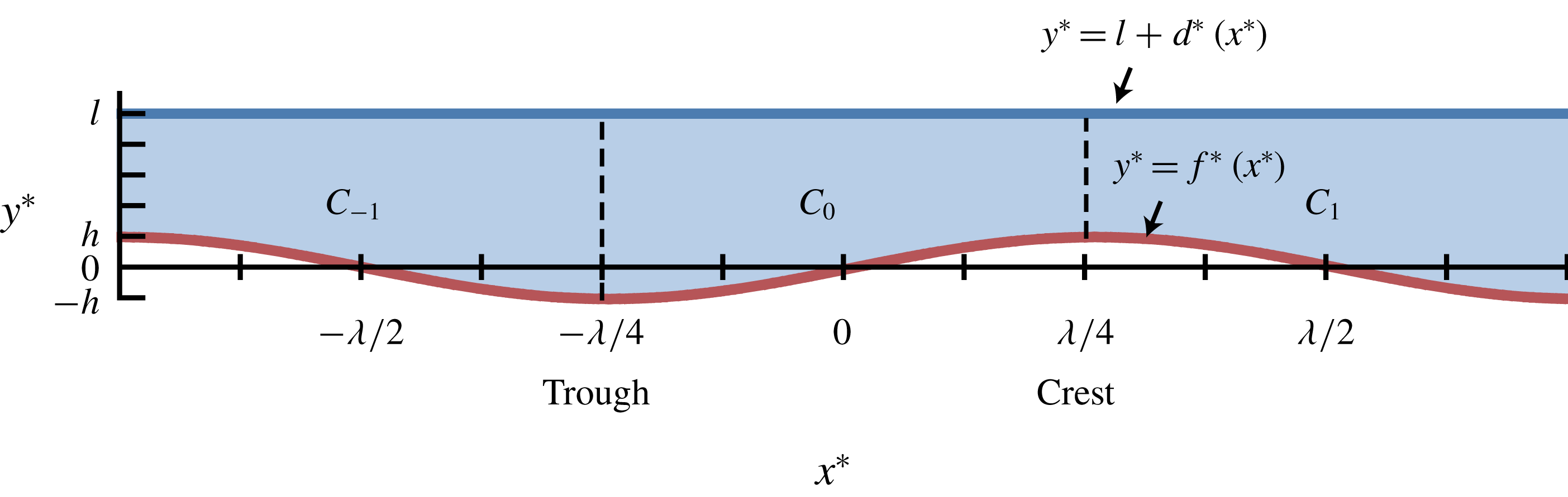
The liquid layer is coated over the substrate and aligned in the $x^{\ast }$ direction. The sinusoidal function describing the shape of the substrate is

(2.1)

$$\begin{eqnarray}f^{\ast }(x^{\ast })=h\sin \frac{2\unicode[STIX]{x03C0}}{\unicode[STIX]{x1D706}}x^{\ast },\end{eqnarray}$$

where $h$ is the amplitude and $\unicode[STIX]{x1D706}$ is the wavelength. Therefore, the substrate has troughs located at $x^{\ast }=n\unicode[STIX]{x1D706}-\unicode[STIX]{x1D706}/4$ and crests at $x^{\ast }=n\unicode[STIX]{x1D706}+\unicode[STIX]{x1D706}/4$ , where $n$ is an arbitrary integer. The vertical location of the interface is $y^{\ast }=l+d^{\ast }(x^{\ast })$ . The mean layer depth, when the interface is flat, is defined by $l$ , and $d^{\ast }(x^{\ast })$ is the disturbance from the flat interface.

The flow domain is horizontally unbounded, and it has symmetry and periodicity in the horizontal direction over the substrate with sinusoidal topography. One can define a unit cell region $C_{n}$ bounded by $x^{\ast }=n\unicode[STIX]{x1D706}/2-\unicode[STIX]{x1D706}/4$ and $x^{\ast }=n\unicode[STIX]{x1D706}/2+\unicode[STIX]{x1D706}/4$ as a primary repeating building block of the flow domain. Adjacent $C_{n}$ and $C_{n+1}$ are symmetric across the vertical boundaries located at troughs or crests of the substrate, and $C_{n}$ and $C_{n+2}$ are periodic in every other cell. An example of the unit cells $C_{-1},C_{0}$ , and $C_{1}$ is depicted in figure 1.

Figure 1.

Flow domain over the substrate with sinusoidal topography. $C_{n}$ represents the $n$ th unit cell and the dashed vertical lines are the boundaries between the unit cells. See text for the $x^{\ast }$ range defined for each cell.

$A$ is defined as the aspect ratio of $C_{n}$ multiplied by $\unicode[STIX]{x03C0}$ :

(2.2)

$$\begin{eqnarray}A=\unicode[STIX]{x03C0}\frac{l}{\unicode[STIX]{x1D706}/2},\end{eqnarray}$$

and the ratio of the amplitude of the substrate topography to the mean depth of the liquid is

(2.3)

$$\begin{eqnarray}H=\frac{h}{l}.\end{eqnarray}$$

Two-dimensional steady flows in the absence of gravity are governed by energy, momentum and mass conservation equations (Sen & Davis Reference Sen and Davis1982; Strani et al. Reference Strani, Piva and Graziani1983):

(2.4)

$$\begin{eqnarray}\displaystyle & \displaystyle u^{\ast }\frac{\unicode[STIX]{x2202}T^{\ast }}{\unicode[STIX]{x2202}x^{\ast }}+v^{\ast }\frac{\unicode[STIX]{x2202}T^{\ast }}{\unicode[STIX]{x2202}y^{\ast }}=\unicode[STIX]{x1D705}\unicode[STIX]{x1D6FB}^{\ast 2}T^{\ast }, & \displaystyle\end{eqnarray}$$

(2.5)

$$\begin{eqnarray}\displaystyle & \displaystyle u^{\ast }\frac{\unicode[STIX]{x2202}u^{\ast }}{\unicode[STIX]{x2202}x^{\ast }}+v^{\ast }\frac{\unicode[STIX]{x2202}u^{\ast }}{\unicode[STIX]{x2202}y^{\ast }}=-\frac{1}{\unicode[STIX]{x1D70C}}\frac{\unicode[STIX]{x2202}p^{\ast }}{\unicode[STIX]{x2202}x^{\ast }}+\unicode[STIX]{x1D708}\unicode[STIX]{x1D6FB}^{\ast 2}u^{\ast }, & \displaystyle\end{eqnarray}$$

(2.6)

$$\begin{eqnarray}\displaystyle & \displaystyle u^{\ast }\frac{\unicode[STIX]{x2202}v^{\ast }}{\unicode[STIX]{x2202}x^{\ast }}+v^{\ast }\frac{\unicode[STIX]{x2202}v^{\ast }}{\unicode[STIX]{x2202}y^{\ast }}=-\frac{1}{\unicode[STIX]{x1D70C}}\frac{\unicode[STIX]{x2202}p^{\ast }}{\unicode[STIX]{x2202}y^{\ast }}+\unicode[STIX]{x1D708}\unicode[STIX]{x1D6FB}^{\ast 2}v^{\ast }, & \displaystyle\end{eqnarray}$$

(2.7)

$$\begin{eqnarray}\displaystyle & \displaystyle \frac{\unicode[STIX]{x2202}u^{\ast }}{\unicode[STIX]{x2202}x^{\ast }}+\frac{\unicode[STIX]{x2202}v^{\ast }}{\unicode[STIX]{x2202}y^{\ast }}=0, & \displaystyle\end{eqnarray}$$

where $p^{\ast }$ , $T^{\ast }$ , $u^{\ast }$ and $v^{\ast }$ are the pressure, temperature and horizontal and vertical velocity components, respectively. $\unicode[STIX]{x1D705}$ , $\unicode[STIX]{x1D70C}$ and $\unicode[STIX]{x1D708}$ are the thermal diffusivity, liquid density and kinematic viscosity, respectively, at the reference temperature $T^{r\ast }$ of the liquid. Introducing the stream function $\unicode[STIX]{x1D713}^{\ast }$ defined by

(2.8a,b )

$$\begin{eqnarray}u^{\ast }=\frac{\unicode[STIX]{x2202}\unicode[STIX]{x1D713}^{\ast }}{\unicode[STIX]{x2202}y^{\ast }},\quad v^{\ast }=-\frac{\unicode[STIX]{x2202}\unicode[STIX]{x1D713}^{\ast }}{\unicode[STIX]{x2202}x^{\ast }},\end{eqnarray}$$

one can reduce (2.5), (2.6) and (2.7) to

(2.9)

$$\begin{eqnarray}\displaystyle & \displaystyle \frac{\unicode[STIX]{x2202}\unicode[STIX]{x1D713}^{\ast }}{\unicode[STIX]{x2202}y^{\ast }}\frac{\unicode[STIX]{x2202}\unicode[STIX]{x1D714}^{\ast }}{\unicode[STIX]{x2202}x^{\ast }}-\frac{\unicode[STIX]{x2202}\unicode[STIX]{x1D713}^{\ast }}{\unicode[STIX]{x2202}x^{\ast }}\frac{\unicode[STIX]{x2202}\unicode[STIX]{x1D714}^{\ast }}{\unicode[STIX]{x2202}y^{\ast }}=\unicode[STIX]{x1D708}\unicode[STIX]{x1D6FB}^{\ast 2}\unicode[STIX]{x1D714}^{\ast }, & \displaystyle\end{eqnarray}$$

(2.10)

$$\begin{eqnarray}\displaystyle & \displaystyle \unicode[STIX]{x1D714}^{\ast }=-\frac{\unicode[STIX]{x2202}^{2}\unicode[STIX]{x1D713}^{\ast }}{\unicode[STIX]{x2202}{x^{\ast }}^{2}}-\frac{\unicode[STIX]{x2202}^{2}\unicode[STIX]{x1D713}^{\ast }}{\unicode[STIX]{x2202}{y^{\ast }}^{2}}, & \displaystyle\end{eqnarray}$$

where $\unicode[STIX]{x1D714}^{\ast }$ is the vorticity.

The liquid layer is heated from below by the substrate of uniform temperature $T^{s\ast }$ and is cooled by a gas of the bulk temperature $T^{g\ast }$ above the layer. Here, we shall use the linear equation of state for surface tension with respect to temperature:

(2.11)

$$\begin{eqnarray}\unicode[STIX]{x1D70E}(T^{\ast })=\unicode[STIX]{x1D70E}_{0}-\unicode[STIX]{x1D6FE}(T^{\ast }-T^{i\ast }),\end{eqnarray}$$

where $\unicode[STIX]{x1D6FE}=-\text{d}\unicode[STIX]{x1D70E}/\text{d}T^{\ast }>0$ and $\unicode[STIX]{x1D70E}_{0}$ is the surface tension at a characteristic temperature at the interface $T^{i\ast }$ (Sen & Davis Reference Sen and Davis1982). The liquid layer satisfies a no-slip condition at the substrate and a stress jump at the gas/liquid interface in the normal and the tangential directions. Therefore, the corresponding vertical boundary conditions for (2.4) and (2.9) are

(2.12)

$$\begin{eqnarray}\displaystyle & \displaystyle -\boldsymbol{n}\boldsymbol{\cdot }\unicode[STIX]{x1D735}^{\ast }(k_{l}T^{\ast })=h_{i}(T^{\ast }-T^{g\ast }),\quad \text{on}~y^{\ast }=l+d^{\ast }(x^{\ast }), & \displaystyle\end{eqnarray}$$

(2.13)

$$\begin{eqnarray}\displaystyle & T^{\ast }=T^{s\ast },\quad \text{on}~y^{\ast }=f^{\ast }(x^{\ast }), & \displaystyle\end{eqnarray}$$

(2.14)

$$\begin{eqnarray}\displaystyle & \left.\begin{array}{@{}c@{}}\boldsymbol{n}\boldsymbol{n}\boldsymbol{ : }\unicode[STIX]{x1D64E}^{\ast }=\unicode[STIX]{x1D70E}K^{\ast },\\ \boldsymbol{n}\boldsymbol{t}\boldsymbol{ : }\unicode[STIX]{x1D64E}^{\ast }=-\unicode[STIX]{x1D6FE}(\boldsymbol{t}\boldsymbol{\cdot }\unicode[STIX]{x1D735}^{\ast }T^{\ast }),\\ \displaystyle v^{\ast }=u^{\ast }\frac{\unicode[STIX]{x2202}d^{\ast }}{\unicode[STIX]{x2202}x^{\ast }},\end{array}\right\}\quad \text{on}~y^{\ast }=l+d^{\ast }(x^{\ast }), & \displaystyle\end{eqnarray}$$

(2.15)

$$\begin{eqnarray}\displaystyle & \displaystyle \unicode[STIX]{x1D713}^{\ast }=\frac{\unicode[STIX]{x2202}\unicode[STIX]{x1D713}^{\ast }}{\unicode[STIX]{x2202}y^{\ast }}=0,\quad \text{on}~y^{\ast }=f^{\ast }(x^{\ast }), & \displaystyle\end{eqnarray}$$

where $\unicode[STIX]{x1D64E}^{\ast }=-p^{\ast }\unicode[STIX]{x1D644}+2\unicode[STIX]{x1D707}\unicode[STIX]{x1D63F}^{\ast }$ is the stress tensor of the liquid; the strain rate tensor $\unicode[STIX]{x1D63F}^{\ast }$ is defined by

(2.16)

$$\begin{eqnarray}\unicode[STIX]{x1D63F}^{\ast }=\left[\begin{array}{@{}cc@{}}\displaystyle \frac{\unicode[STIX]{x2202}u^{\ast }}{\unicode[STIX]{x2202}x^{\ast }} & \displaystyle \frac{1}{2}\left(\frac{\unicode[STIX]{x2202}u^{\ast }}{\unicode[STIX]{x2202}y^{\ast }}+\frac{\unicode[STIX]{x2202}v^{\ast }}{\unicode[STIX]{x2202}x^{\ast }}\right)\\ \displaystyle \frac{1}{2}\left(\frac{\unicode[STIX]{x2202}u^{\ast }}{\unicode[STIX]{x2202}y^{\ast }}+\frac{\unicode[STIX]{x2202}v^{\ast }}{\unicode[STIX]{x2202}x^{\ast }}\right) & \displaystyle \frac{\unicode[STIX]{x2202}v^{\ast }}{\unicode[STIX]{x2202}y^{\ast }}\end{array}\right].\end{eqnarray}$$

$\unicode[STIX]{x1D707}$ , $k_{l}$ and $h_{i}$ are the dynamic viscosity of the liquid, heat conductivity of the liquid and heat transfer coefficient of the gas side near the interface, respectively, all referred to $T^{r\ast }$ . The unit outward normal vector $\boldsymbol{n}$ , unit tangent vector $\boldsymbol{t}$ and curvature $K^{\ast }$ of the interface are given by

(2.17a-c )

$$\begin{eqnarray}\boldsymbol{n}=\frac{1}{N}\left(-\frac{\unicode[STIX]{x2202}d^{\ast }}{\unicode[STIX]{x2202}x^{\ast }}\quad 1\right),\quad \boldsymbol{t}=\frac{1}{N}\left(1\quad \frac{\unicode[STIX]{x2202}d^{\ast }}{\unicode[STIX]{x2202}x^{\ast }}\right),\quad K^{\ast }=\frac{1}{N^{3}}\frac{\unicode[STIX]{x2202}^{2}d^{\ast }}{\unicode[STIX]{x2202}{x^{\ast }}^{2}},\end{eqnarray}$$

where $N=[1+(\unicode[STIX]{x2202}d^{\ast }/\unicode[STIX]{x2202}x^{\ast })^{2}]^{1/2}$ . Note that there is no horizontal boundary. Therefore, the temperature and flow fields inherit the symmetry and periodicity of the flow domain.

Apart from the above boundary conditions, the mass is conserved at any $x^{\ast }$ , which leads to the condition of no net mass flow (Sen & Davis Reference Sen and Davis1982):

(2.18)

$$\begin{eqnarray}\int _{f^{\ast }(x^{\ast })}^{l+d^{\ast }(x^{\ast })}u^{\ast }\,\text{d}y^{\ast }=0.\end{eqnarray}$$

This produces the additional boundary condition for the stream function

(2.19)

$$\begin{eqnarray}\unicode[STIX]{x1D713}^{\ast }=0,\quad \text{on}~y^{\ast }=l+d^{\ast }(x^{\ast }).\end{eqnarray}$$

The characteristic temperature $T^{i\ast }$ and temperature difference $\unicode[STIX]{x0394}T^{i\ast }$ at the interface are defined under the assumption of purely vertical heat diffusion inside the liquid layer and the flat interface. Since $f^{\ast }$ is small compared to $l$ , the continuity of the heat fluxes inside of and at the surface of the liquid layer approximately satisfies the following relation,

(2.20)

$$\begin{eqnarray}k_{l}\frac{T^{s\ast }-T^{\ast }|_{y^{\ast }=l}}{l-f^{\ast }}\approx h_{i}(T^{i\ast }-T^{g\ast }).\end{eqnarray}$$

For $T^{\ast }|_{y^{\ast }=l}$ , rearranging (2.20),

(2.21)

$$\begin{eqnarray}T^{\ast }|_{y^{\ast }=l}\approx T^{s\ast }-\mathit{Bi}\left(1-\frac{f^{\ast }}{l}\right)(T^{i\ast }-T^{g\ast }).\end{eqnarray}$$

$\mathit{Bi}=h_{i}l/k_{l}$ is the Biot number that represents the ratio of the heat transfer resistances inside of and at the surface of a liquid layer. $T^{i\ast }$ and $\unicode[STIX]{x0394}T^{i\ast }$ are defined as the temperature at the interface with $f^{\ast }=0$ and the temperature difference between $T^{it\ast }$ and $T^{ic\ast }$ , respectively. Herein, $T^{it\ast }$ and $T^{ic\ast }$ are the temperatures at the interface above the trough ( $f^{\ast }=-h$ ) and crest ( $f^{\ast }=h$ ), respectively, of the substrate. Using (2.21), the characteristic variables are defined as

(2.22)

$$\begin{eqnarray}\displaystyle & \displaystyle T^{i\ast }=\frac{T^{s\ast }+\mathit{Bi}\,T^{g\ast }}{1+\mathit{Bi}}, & \displaystyle\end{eqnarray}$$

(2.23)

$$\begin{eqnarray}\displaystyle & \unicode[STIX]{x0394}T^{i\ast }=2H(T^{s\ast }-T^{i\ast }). & \displaystyle\end{eqnarray}$$

Here, we scale the system by introducing the following quantities:

(2.24a-f )

$$\begin{eqnarray}x=\frac{x^{\ast }}{\unicode[STIX]{x1D706}/2\unicode[STIX]{x03C0}},\quad y=\frac{y^{\ast }}{l},\quad u=\frac{u^{\ast }}{U},\quad v=\frac{v^{\ast }}{AU},\quad p=\frac{p^{\ast }}{\unicode[STIX]{x1D707}U\unicode[STIX]{x1D706}/2\unicode[STIX]{x03C0}l^{2}},\quad T=\frac{T^{\ast }-T^{i\ast }}{\unicode[STIX]{x0394}T^{i\ast }}.\end{eqnarray}$$

Using these variables, the characteristic velocity of the system $U$ can be derived from the balance between the jump in shear stress along the interface and the surface-tension gradient (Sen & Davis Reference Sen and Davis1982):

(2.25)

$$\begin{eqnarray}U=\frac{\unicode[STIX]{x1D6FE}\unicode[STIX]{x0394}T^{i\ast }}{\unicode[STIX]{x1D707}}A.\end{eqnarray}$$

Using the above scaling, the function describing the substrate becomes

(2.26)

$$\begin{eqnarray}f(x)=H\hat{f}(x)=H\sin x,\end{eqnarray}$$

where the dimensionless wavelength and amplitude are $2\unicode[STIX]{x03C0}$ and $H$ , respectively. Therefore, $C_{n}$ is bounded by $x=n\unicode[STIX]{x03C0}-\unicode[STIX]{x03C0}/2$ and $x=n\unicode[STIX]{x03C0}+\unicode[STIX]{x03C0}/2$ . The normalised substrate shape is defined by $\hat{f}(x)=\sin x$ . In this study, we consider $H=O(0.1)$ . The geometry of the liquid layer is defined by $A$ and $H$ .

The dimensionless governing equations can be written as follows:

(2.27)

$$\begin{eqnarray}\displaystyle & \mathit{Ma}\,A(\unicode[STIX]{x1D713}_{y}T_{x}-\unicode[STIX]{x1D713}_{x}T_{y})=A^{2}T_{xx}+T_{yy}, & \displaystyle\end{eqnarray}$$

(2.28)

$$\begin{eqnarray}\displaystyle & \mathit{Re}\,A(\unicode[STIX]{x1D713}_{y}\unicode[STIX]{x1D714}_{x}-\unicode[STIX]{x1D713}_{x}\unicode[STIX]{x1D714}_{y})=A^{2}\unicode[STIX]{x1D714}_{xx}+\unicode[STIX]{x1D714}_{yy}, & \displaystyle\end{eqnarray}$$

(2.29)

$$\begin{eqnarray}\displaystyle & \unicode[STIX]{x1D714}=-A^{2}\unicode[STIX]{x1D713}_{xx}-\unicode[STIX]{x1D713}_{yy}. & \displaystyle\end{eqnarray}$$

The Marangoni number $\mathit{Ma}$ , Reynolds number $\mathit{Re}$ , Prandtl number $\mathit{Pr}$ and capillary number $\mathit{Ca}$ are defined by

(2.30a-d )

$$\begin{eqnarray}\displaystyle \mathit{Ma}=\frac{Ul}{\unicode[STIX]{x1D705}},\quad \mathit{Re}=\frac{Ul}{\unicode[STIX]{x1D708}},\quad \mathit{Pr}=\frac{\unicode[STIX]{x1D708}}{\unicode[STIX]{x1D705}},\quad \mathit{Ca}=\frac{\unicode[STIX]{x1D707}U}{\unicode[STIX]{x1D70E}_{0}}\end{eqnarray}$$

and $\mathit{Re}=\mathit{Ma}/\mathit{Pr}$ . The boundary conditions (2.12)–(2.15) transform to

(2.31)

$$\begin{eqnarray}\displaystyle & \displaystyle \frac{T_{y}-A^{2}d_{x}T_{x}}{(1+A^{2}d_{x}^{2})^{1/2}}=-\mathit{Bi}\,T-\frac{1}{2H},\quad \text{on}~y=1+d(x), & \displaystyle\end{eqnarray}$$

(2.32)

$$\begin{eqnarray}\displaystyle & \displaystyle T=\frac{1}{2H},\quad \text{on}~y=f(x), & \displaystyle\end{eqnarray}$$

(2.33)

$$\begin{eqnarray}\displaystyle & \left.\begin{array}{@{}c@{}}\displaystyle -p+\frac{2A^{2}}{(1+A^{2}d_{x}^{2})}[(v_{y}-d_{x}u_{y})+A^{2}d_{x}(-v_{x}+d_{x}u_{x})]\\ \displaystyle =\frac{A^{2}d_{xx}}{(1+A^{2}d_{x}^{2})^{3/2}}\left(\frac{A}{\mathit{Ca}}-T\right),\qquad \qquad \quad \\ \displaystyle (u_{y}+A^{2}v_{x})(1-A^{2}d_{x}^{2})+2A^{2}d_{x}(v_{y}-u_{x})\\ \displaystyle =-(1+A^{2}d_{x}^{2})^{1/2}(T_{x}+d_{x}T_{y}),\quad \\ v=ud_{x},\end{array}\right\}\quad \text{on}~y=1+d(x), & \displaystyle\end{eqnarray}$$

(2.34)

$$\begin{eqnarray}\displaystyle & \unicode[STIX]{x1D713}=\unicode[STIX]{x1D713}_{y}=0,\quad \text{on}~y=f(x), & \displaystyle\end{eqnarray}$$

and the condition of no net mass flow (2.19) becomes

(2.35)

$$\begin{eqnarray}\unicode[STIX]{x1D713}=0,\quad \text{on}~y=1+d(x).\end{eqnarray}$$

3 Asymptotic solutions

The liquid layer system considered in this study has a small $A$ , i.e. $A\ll 1$ . In particular, we treat the system in the asymptotic limit as $A\rightarrow 0$ . In this limit, the complete temperature and flow fields may be determined by a regular perturbation of (2.27)–(2.29) and (2.31)–(2.35) in a small perturbation quantity $A$ . The solutions can be described by asymptotic expansions with the asymptotic sequence $\{A^{m}\}$ , where $m$ is an integer, as $A\rightarrow 0$ :

(3.1)

$$\begin{eqnarray}\left.\begin{array}{@{}c@{}}T(x,y)=T_{0}(x,y)+AT_{1}(x,y)+A^{2}T_{2}(x,y)+\cdots ,\\ \unicode[STIX]{x1D714}(x,y)=\unicode[STIX]{x1D714}_{0}(x,y)+A\unicode[STIX]{x1D714}_{1}(x,y)+A^{2}\unicode[STIX]{x1D714}_{2}(x,y)+\cdots ,\\ \unicode[STIX]{x1D713}(x,y)=\unicode[STIX]{x1D713}_{0}(x,y)+A\unicode[STIX]{x1D713}_{1}(x,y)+A^{2}\unicode[STIX]{x1D713}_{2}(x,y)+\cdots ,\\ p(x,y)=p_{0}(x,y)+Ap_{1}(x,y)+A^{2}p_{2}(x,y)+\cdots ,\\ d(x)=Ad_{1}(x)+A^{2}d_{2}(x)+\cdots ,\end{array}\right\}\end{eqnarray}$$

and $u(x,y)$ and $v(x,y)$ can be derived from (2.8). Using the expansions, the solutions of the governing equations can be obtained by a systematic scheme of successive approximations (Van Dyke Reference Van Dyke1964). In the present work, the second-order solutions are investigated. They are sufficient to describe the temperature and flow fields when compared with the numerical solutions described in § 4. We obtain the solutions applicable over the entire liquid layer, but the solutions are depicted in $C_{0}$ only.

In this study, the analysis is based on the following asymptotic limits of the dimensionless parameters:

(3.2a-c )

$$\begin{eqnarray}\mathit{Ma}=\overline{\mathit{Ma}}\,A,\quad \mathit{Re}=\overline{\mathit{Re}}\,A,\quad \mathit{Ca}=\overline{\mathit{Ca}}\,A^{6},\end{eqnarray}$$

with $\overline{\mathit{Ma}}$ , $\overline{\mathit{Re}}$ and $\overline{\mathit{Ca}}$ of $O(1)$ . The order of $A$ in $\mathit{Ma}$ and $\mathit{Re}$ , which implies $\mathit{Pr}=O(1)$ , corresponds to mild heating and slow liquid convections. The convection terms appear from the second corrections onward.

Given equation (2.25), the capillary number used here can be interpreted as a crispation number relating the effect of the surface-tension gradient to that of the surface tension, and $\mathit{Ca}=O(A^{6})$ implies that a high surface tension stabilises a flat interface in this system. For organic liquids used in liquid film coatings, $\mathit{Ca}$ has the order of $10^{-2}\unicode[STIX]{x0394}T^{i\ast }A$ based on the material properties in Kőrösi & Kováts (Reference Kőrösi and Kováts1981), Poling et al. (Reference Poling, Thomson, Friend, Rowley, Wilding and Maloney2008). Therefore, the proposed model is physically relevant when the order of $\unicode[STIX]{x0394}T^{i\ast }$ becomes $10^{2}{A^{5}\,}^{\circ }\,\text{C}$ , for satisfying $\mathit{Ca}=O(A^{6})$ . For example, using a toluene solution based on the material properties of toluene in Kőrösi & Kováts (Reference Kőrösi and Kováts1981) with $l=0.1~\text{mm}$ , $\unicode[STIX]{x1D706}/2\unicode[STIX]{x03C0}=0.5~\text{mm}$ , and hence $A=0.2$ , the system is required to have $\unicode[STIX]{x0394}T^{i\ast }\approx 0.1\,^{\circ }\text{C}$ .

Considering the order of $\mathit{Ca}$ , the jump in the normal stress from (2.33) leads to

(3.3a,b )

$$\begin{eqnarray}d_{1}=0,\quad d_{2}=0,\end{eqnarray}$$

and the first non-trivial correction appears at $O(A^{3})$ . In the second-order solutions, the disturbance of the interface shape vanishes, and therefore, the position of the interface is fixed, which proves that the flat interface is relevant. In addition, the steady-state solutions in this study are stable due to the order of $\mathit{Ca}$ when applying a usual procedure for linear stability analysis in Oron, Davis & Bankoff (Reference Oron, Davis and Bankoff1997) and Pham et al. (Reference Pham, Cheng and Kumar2017).

From the normal stress condition, the third and higher corrections for the interface shape can be calculated, such as $d_{3,xx}(x)=-p_{0}$ in the leading order. As only the second-order solutions are considered in this study, the normal stress condition need not be treated. Using (3.3), the kinematic condition in (2.33) leads to

(3.4a-c )

$$\begin{eqnarray}v_{0}=0,\quad v_{1}=0,\quad v_{2}=0,\quad \text{on}~y=1,\end{eqnarray}$$

which is compatible with the condition of no net mass flow (2.35). Thus, only the jump in the tangential stress needs to be considered for the second-order solutions. $\mathit{Bi}$ is chosen as $O(1)$ , as used in other studies (Sen & Davis Reference Sen and Davis1982; Eckert et al. Reference Eckert, Bestehorn and Thess1998).

3.1 Basic solutions

Substituting the expansions (3.1) into (2.27)–(2.29) and (2.31)–(2.35), we find the leading-order equations

(3.5)

$$\begin{eqnarray}\displaystyle & T_{0,yy}=0, & \displaystyle\end{eqnarray}$$

(3.6)

$$\begin{eqnarray}\displaystyle & \unicode[STIX]{x1D714}_{0,yy}=0, & \displaystyle\end{eqnarray}$$

(3.7)

$$\begin{eqnarray}\displaystyle & \unicode[STIX]{x1D714}_{0}=-\unicode[STIX]{x1D713}_{0,yy}, & \displaystyle\end{eqnarray}$$

with the boundary conditions

(3.8)

$$\begin{eqnarray}\displaystyle & \displaystyle T_{0,y}=-\mathit{Bi}\,T_{0}-\frac{1}{2H},\quad \text{on}~y=1, & \displaystyle\end{eqnarray}$$

(3.9)

$$\begin{eqnarray}\displaystyle & \displaystyle T_{0}=\frac{1}{2H},\quad \text{on}~y=f(x), & \displaystyle\end{eqnarray}$$

(3.10)

$$\begin{eqnarray}\displaystyle & \unicode[STIX]{x1D714}_{0}=T_{0,x},\quad \text{on}~y=1, & \displaystyle\end{eqnarray}$$

(3.11)

$$\begin{eqnarray}\displaystyle & \unicode[STIX]{x1D713}_{0}=\unicode[STIX]{x1D713}_{0,y}=0,\quad \text{on}~y=f(x), & \displaystyle\end{eqnarray}$$

where the interfacial vorticity is defined by $\unicode[STIX]{x1D714}_{0}|_{y=1}=-u_{0,y}|_{y=1}$ in (3.10), and the condition of no net mass flow

(3.12)

$$\begin{eqnarray}\unicode[STIX]{x1D713}_{0}=0,\quad \text{on}~y=1.\end{eqnarray}$$

The governing equations (3.5) and (3.6) show that the vertical diffusion is the only transport mechanism of heat and vorticity for the basic solutions. Equations (3.9) and (3.10) indicate that the heat and vorticity arise from the substrate and the interface, respectively.

The solution for $T_{0}$ that satisfies (3.5), (3.8) and (3.9) is

(3.13)

$$\begin{eqnarray}T_{0}(x,y)=\unicode[STIX]{x1D719}_{0}(x)\,\bar{T}_{0}(y)-\frac{1}{2\mathit{Bi}\,H},\end{eqnarray}$$

where

(3.14)

$$\begin{eqnarray}\bar{T}_{0}(y)=-y+1+\frac{1}{\mathit{Bi}},\end{eqnarray}$$

and

(3.15)

$$\begin{eqnarray}\unicode[STIX]{x1D719}_{0}(x)=\frac{1+\mathit{Bi}}{2H(1+\mathit{Bi}-\mathit{Bi}\,f(x))}.\end{eqnarray}$$

In this study, we approximate the results from asymptotic solutions for a small magnitude $H=O(0.1)$ in order to interpret the effects of substrate topography and the heat-transfer characteristics on the temperature and flow fields. The approximation is based on Taylor series expansions with respect to $H$ around $H=0$ . For $\unicode[STIX]{x1D719}_{0}(x)$ , the expression $H\unicode[STIX]{x1D719}_{0}(x)$ is approximated, and the terms up to the order of $H$ are retained:

(3.16)

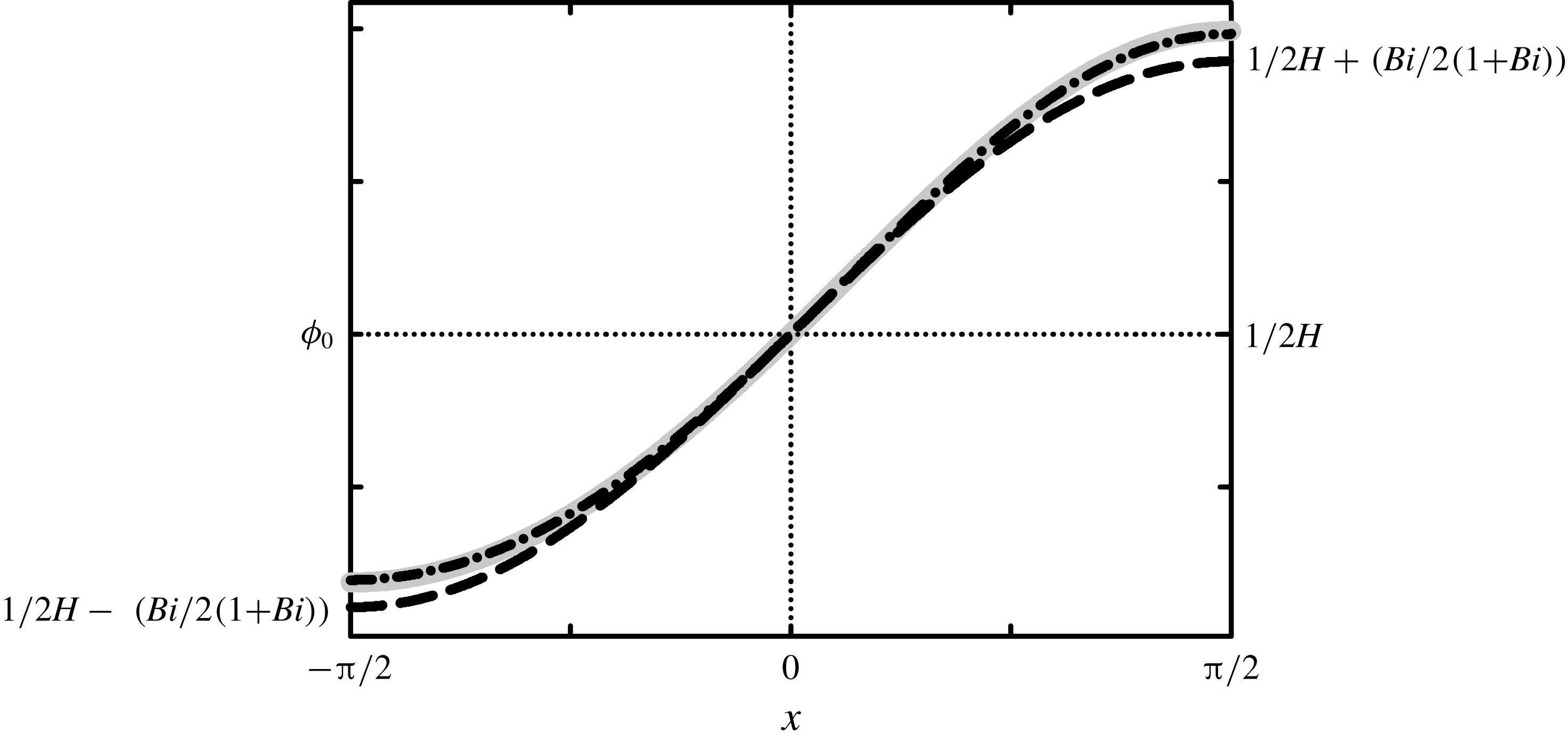
$$\begin{eqnarray}\unicode[STIX]{x1D719}_{0}(x)\approx \frac{1}{2H}+\frac{\mathit{Bi}}{2(1+\mathit{Bi})}\hat{f}(x)+\frac{\mathit{Bi}^{2}}{2(1+\mathit{Bi})^{2}}\hat{f}^{2}(x)H.\end{eqnarray}$$

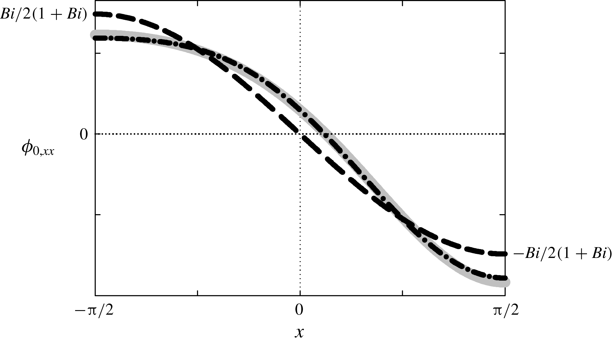
According to figure 2, this linear approximation is reasonable for this study.

Figure 2.

Heat flux $\unicode[STIX]{x1D719}_{0}(x)$ for $\mathit{Bi}=1$ and $H=0.2$ : —— (grey), exact one in (3.15); – – –, zeroth order approximation in $H$ from (3.16); – ⋅ – ⋅ –, linear approximation in $H$ in (3.16).

The vertical heat diffusion causes $T_{0}$ to linearly depend on $y$ , as shown in $\bar{T}_{0}(y)$ . Meanwhile, the dependence of $T_{0}$ on $x$ is isolated in $\unicode[STIX]{x1D719}_{0}(x)$ , which is essentially the dimensionless heat flux, $-T_{0,y}$ . $f(x)$ causes $\unicode[STIX]{x1D719}_{0}(x)$ to increase along $x$ in $C_{0}$ , as indicated by (3.15). The first term in (3.16) is the base value and the second term shows that the flux depends on $\hat{f}(x)$ , and the amplitude of the second term is $(1/2)\mathit{Bi}(1+\mathit{Bi})^{-1}$ . According to figure 2, $\unicode[STIX]{x1D719}_{0}(x)$ can be adequately described by using the zeroth approximation in $H$ . Therefore, $\unicode[STIX]{x1D719}_{0}(x)$ mainly reflects the effect of the normalised substrate shape and the ratio of the internal to external heat transfer resistance of the liquid layer on $T_{0}$ . The remaining linear contribution in $H$ affects $\unicode[STIX]{x1D719}_{0}(x)$ slightly. 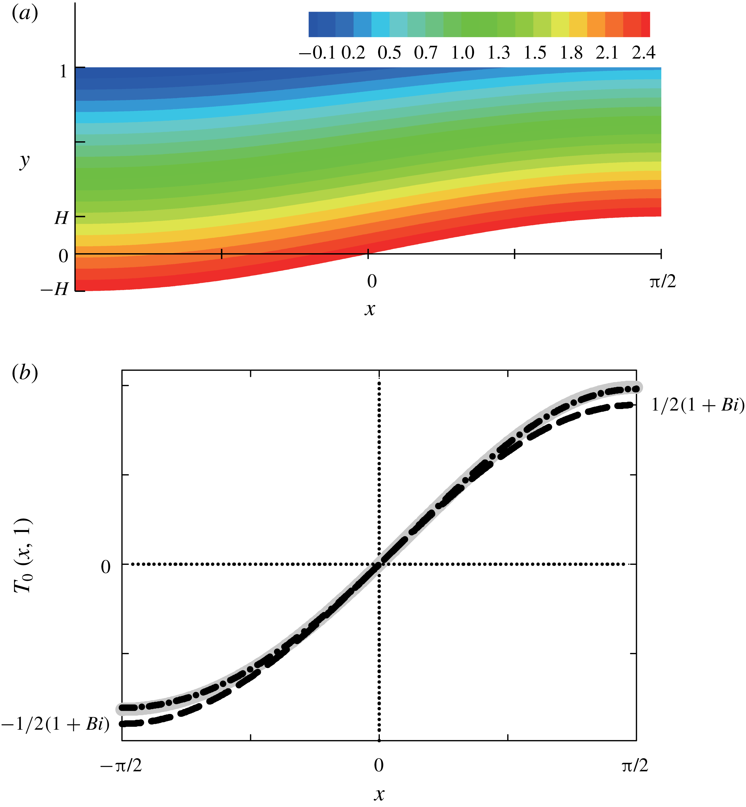Consequently, $\bar{T}_{0}(y)$ controls the temperature vertically, and $\unicode[STIX]{x1D719}_{0}(x)$ does so horizontally, as shown in the temperature field for the basic solution depicted in figure 3(a).

Figure 3.

(a) Contour plot of $T_{0}$ , and (b) $T_{0}(x,1)$ profile corresponding to $x$ : —— (grey), exact one in (3.17a ); – – –, zeroth order approximation in $H$ from (3.17b ); – ⋅ – ⋅ –, linear approximation in $H$ in (3.17b ). $\mathit{Bi}=1$ and $H=0.2$ for all plots.

As we discussed, the chief cause of flows is the thermocapillary force, which is generated by the non-uniform interfacial temperature. The interfacial temperature is

(3.17a )

$$\begin{eqnarray}\displaystyle T_{0}(x,1) & = & \displaystyle \frac{f(x)}{2H(1+\mathit{Bi}-\mathit{Bi}\,f(x))}\end{eqnarray}$$

(3.17b )

$$\begin{eqnarray}\displaystyle & {\approx} & \displaystyle \frac{1}{2(1+\mathit{Bi})}\hat{f}(x)+\frac{\mathit{Bi}}{2(1+\mathit{Bi })^{2}}\hat{f}^{2}(x)H.\end{eqnarray}$$

As expected,

$f(x)$ causes

$T_{0}(x,1)$ to increase along

$x$ in

$C_{0}$ , as shown in (3.17a ). Figure 3(b) shows that the

$T_{0}(x,1)$ profile can be adequately described by using the zeroth approximation in

$H$ . The first term in equation (3.17b ) shows that the normalised substrate shape mainly governs the interfacial

$T_{0}$ profile with its amplitude

$(1/2)(1+\mathit{Bi})^{-1}$ . The remaining linear contribution in

$H$ slightly affects the

$T_{0}(x,1)$ profile.

The interfacial temperature gradient, $T_{0,x}|_{y=1}$ , is

(3.18a )

$$\begin{eqnarray}\displaystyle \unicode[STIX]{x1D6E9}_{0}^{i}(x) & = & \displaystyle \frac{1+\mathit{Bi}}{2H(1+\mathit{Bi}-\mathit{Bi}\,f(x))^{2}}f^{\prime }(x)\end{eqnarray}$$

(3.18b )

$$\begin{eqnarray}\displaystyle & {\approx} & \displaystyle \frac{1}{2(1+\mathit{Bi})}\hat{f}^{\prime }(x)+\frac{\mathit{Bi}}{(1+\mathit{Bi })^{2}}\hat{f}(x)\hat{f}^{\prime }(x)H.\end{eqnarray}$$

$f(x)$ in

$T_{0}(x,1)$ causes the dependence of

$\unicode[STIX]{x1D6E9}_{0}^{i}(x)$ on

$f^{\prime }(x)$ , which induces

$\unicode[STIX]{x1D6E9}_{0}^{i}(x)$ to be always positive in

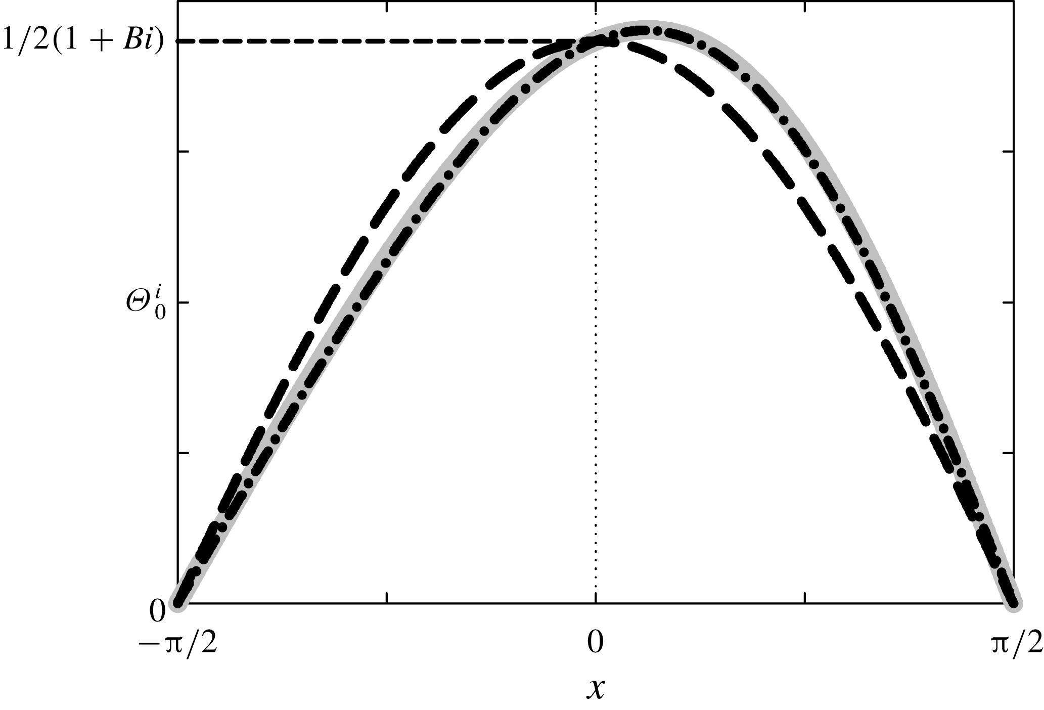
$C_{0}$ , as shown in (3.18a ). Figure 4 shows that the linear approximation in (3.18b ) is reasonable. The first term in (3.18b ) explicitly shows that

$\unicode[STIX]{x1D6E9}_{0}^{i}(x)$ depends on

$\hat{f}^{\prime }(x)$ , in this study

$\cos x$ , which is the normalised substrate slope, and the amplitude of the first term is

$(1/2)(1+\mathit{Bi})^{-1}$ . According to figure 4, the profile of

$\unicode[STIX]{x1D6E9}_{0}^{i}(x)$ can be roughly captured by the zeroth approximation in

$H$ . Therefore,

$\unicode[STIX]{x1D6E9}_{0}^{i}(x)$ is mainly governed by the normalised substrate slope and the ratio of the internal to external heat transfer resistance of the liquid layer. The remaining linear contribution in

$H$ completes

$\unicode[STIX]{x1D6E9}_{0}^{i}(x)$ by marginally disrupting the symmetry across

$x=0$ .

Figure 4.

Interfacial temperature gradient $\unicode[STIX]{x1D6E9}_{0}^{i}(x)$ for $Bi=1$ and $H=0.2$ : —— (grey), exact one in (3.18a ); – – –, zeroth order approximation in $H$ from (3.18b ); – ⋅ – ⋅ –, linear approximation in $H$ in (3.18b ).

According to the boundary condition (3.10), the interfacial vorticity is generated by $\unicode[STIX]{x1D6E9}_{0}^{i}(x)$ . The vorticity propagates via the viscous diffusion, as governed by (3.6), which induces the flows in the leading order. Therefore, $\unicode[STIX]{x1D6E9}_{0}^{i}(x)$ works as the driving force for the flows. As a result, a vortex appears inside the unit cell because flows cannot penetrate the boundaries of the cell, which will be established in this paper.

The solutions for $\unicode[STIX]{x1D714}_{0}$ , $u_{0}$ and $\unicode[STIX]{x1D713}_{0}$ can be obtained by solving (3.6), (3.7) and (3.10)–(3.12). They are

(3.19)

$$\begin{eqnarray}\displaystyle & \unicode[STIX]{x1D714}_{0}(x,Y)=\unicode[STIX]{x1D6E9}_{0}^{i}(x)\,\bar{\unicode[STIX]{x1D714}}_{0}(Y), & \displaystyle\end{eqnarray}$$

(3.20)

$$\begin{eqnarray}\displaystyle & u_{0}(x,Y)=\unicode[STIX]{x1D6E9}_{0}^{i}(x)D(x)\,\bar{u}_{0}(Y), & \displaystyle\end{eqnarray}$$

(3.21)

$$\begin{eqnarray}\displaystyle & \unicode[STIX]{x1D713}_{0}(x,Y)=\unicode[STIX]{x1D6E9}_{0}^{i}(x)D^{2}(x)\,\bar{\unicode[STIX]{x1D713}}_{0}(Y), & \displaystyle\end{eqnarray}$$

where $D(x)=1-f(x)$ is the depth of the liquid layer and $Y=(y-f(x))/D(x)$ is the vertical position rescaled by the depth. Here, we factored out $\unicode[STIX]{x1D6E9}_{0}^{i}(x)$ or $D(x)$ from $\unicode[STIX]{x1D714}_{0}$ , $u_{0}$ and $\unicode[STIX]{x1D713}_{0}$ because, in $x$ and $Y$ coordinates, the effects of the substrate topography lie in $\unicode[STIX]{x1D6E9}_{0}^{i}(x)$ and $D(x)$ . Then, the remaining terms become

(3.22)

$$\begin{eqnarray}\displaystyle & \bar{\unicode[STIX]{x1D714}}_{0}(Y)={\textstyle \frac{3}{2}}\left(Y-{\textstyle \frac{1}{3}}\right), & \displaystyle\end{eqnarray}$$

(3.23)

$$\begin{eqnarray}\displaystyle & \bar{u}_{0}(Y)=-{\textstyle \frac{3}{4}}\left(Y-{\textstyle \frac{2}{3}}\right)Y, & \displaystyle\end{eqnarray}$$

(3.24)

$$\begin{eqnarray}\displaystyle & \bar{\unicode[STIX]{x1D713}}_{0}(Y)=-{\textstyle \frac{1}{4}}(Y-1)Y^{2}. & \displaystyle\end{eqnarray}$$

The vertical vorticity diffusion causes $\unicode[STIX]{x1D714}_{0}$ to linearly depend on $Y$ , as shown in $\bar{\unicode[STIX]{x1D714}}_{0}(Y)$ . Similarly, the dependence of $u$ and $\unicode[STIX]{x1D713}$ on $Y$ appears in $\bar{u}_{0}(Y)$ and $\bar{\unicode[STIX]{x1D713}}_{0}(Y)$ , respectively.

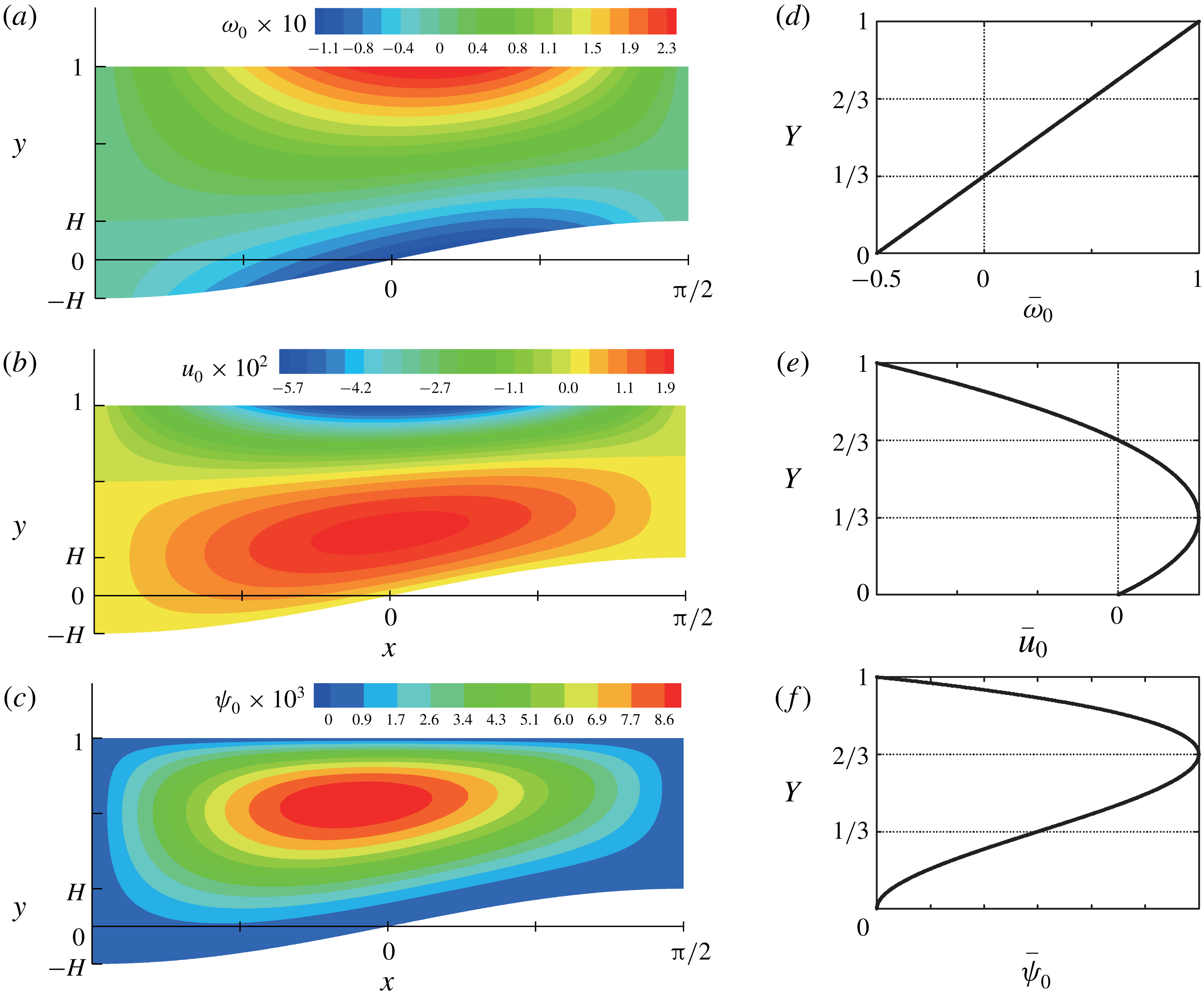
Equation (3.19) can explain the vertical and horizontal changes in $\unicode[STIX]{x1D714}_{0}$ shown in figure 5(a). $\bar{\unicode[STIX]{x1D714}}_{0}(Y)$ vertically controls the vorticity, and $\unicode[STIX]{x1D6E9}_{0}^{i}(x)$ does so horizontally. Figure 5(d) shows that $\bar{\unicode[STIX]{x1D714}}_{0}$ is positive at the interface, decreases linearly as $Y$ decreases, and changes sign at $Y=1/3$ . Because of the no-slip boundary condition, $\bar{\unicode[STIX]{x1D714}}_{0}$ becomes negative near the substrate. As indicated by $\unicode[STIX]{x1D6E9}_{0}^{i}(x)$ , figure 4 implies that the interfacial $\unicode[STIX]{x1D714}_{0}$ has the maximum value near the centre and vanishes at both corners of the interface. Because of the symmetry between neighbouring unit cells, the sign of the vorticity changes across the cell boundaries.

Figure 5.

Contour plots of (a) $\unicode[STIX]{x1D714}_{0}$ , (b) $u_{0}$ and (c) $\unicode[STIX]{x1D713}_{0}$ for $\mathit{Bi}=1$ and $H=0.2$ , and the plots of (d) $\bar{\unicode[STIX]{x1D714}}_{0}(Y)$ , (e) $\bar{u}_{0}(Y)$ and (f) $\bar{\unicode[STIX]{x1D713}}_{0}(Y)$ .

This vorticity profile leads to a typical reversal flow inside the layer, as shown in figure 5(b). The horizontal velocity changes quadratically along $Y$ and has a maximum magnitude at $Y=1/3$ , as plotted in figure 5(e). Note that the flow reversal occurs at $Y=2/3$ . Therefore, the vortex centre, which is characterised by vanishing velocity components, should exist at $Y=2/3$ (Nam, Scriven & Carvalho Reference Nam, Scriven and Carvalho2009). The symmetric substrate topography causes the change in the sign of $\unicode[STIX]{x1D6E9}_{0}^{i}(x)$ and the corresponding change in the direction of the horizontal velocity across the unit cell boundaries.

This reversal flow in the unit cell implies a circular streamline pattern, as shown in figure 5(c). The stream function changes cubically along $Y$ and has the maximum value at $Y=2/3$ and an inflexion point at $Y=1/3$ , as plotted in figure 5(f). The stream function vanishes at the unit cell boundaries because of the absence of the driving force, i.e. $\unicode[STIX]{x1D6E9}_{0}^{i}=0$ . Owing to the no-penetration conditions, the stream function also vanishes on the substrate and the interface. Because the unit cell is surrounded by $\unicode[STIX]{x1D713}_{0}=0$ , the flows cannot penetrate the boundaries of the cell. Note that all the stream function values on $C_{0}$ are positive because $\bar{\unicode[STIX]{x1D713}}_{0}(Y)>0$ and $\unicode[STIX]{x1D6E9}_{0}^{i}(x)>0$ . Therefore, the recirculation direction is anticlockwise. However, the neighbouring cells, $C_{-1}$ and $C_{1}$ , have the opposite recirculation direction, which is due to $\unicode[STIX]{x1D6E9}_{0}^{i}(x)<0$ . The inherent symmetry and periodicity of the solutions permit a straightforward reconstruction of the complete temperature and flow fields in the infinitely long liquid layer.

To summarise, the behaviours of the basic solutions along the vertical direction can be adequately represented by variables with the bar symbol, e.g. $\bar{T}_{0}(y)$ and $\bar{\unicode[STIX]{x1D714}}_{0}(Y)$ . In this study, the heat flux $\unicode[STIX]{x1D719}_{0}(x)$ and the interfacial temperature gradient $\unicode[STIX]{x1D6E9}_{0}^{i}(x)$ clearly show the effect of the substrate shape and slope, respectively, in combination with the ratio of the internal to external heat transfer resistance of the liquid layer on the basic solutions.

3.2 First and second corrections

To the first corrections, $T_{1}$ , $\unicode[STIX]{x1D714}_{1}$ and $\unicode[STIX]{x1D713}_{1}$ satisfy the set of equations

(3.25)

$$\begin{eqnarray}\displaystyle & T_{1,yy}=0, & \displaystyle\end{eqnarray}$$

(3.26)

$$\begin{eqnarray}\displaystyle & \unicode[STIX]{x1D714}_{1,yy}=0, & \displaystyle\end{eqnarray}$$

(3.27)

$$\begin{eqnarray}\displaystyle & \unicode[STIX]{x1D714}_{1}=-\unicode[STIX]{x1D713}_{1,yy}, & \displaystyle\end{eqnarray}$$

together with the boundary conditions

(3.28)

$$\begin{eqnarray}\displaystyle & T_{1,y}=-\mathit{Bi}\,T_{1},\quad \text{on}~y=1, & \displaystyle\end{eqnarray}$$

(3.29)

$$\begin{eqnarray}\displaystyle & T_{1}=0,\quad \text{on}~y=f(x), & \displaystyle\end{eqnarray}$$

(3.30)

$$\begin{eqnarray}\displaystyle & \unicode[STIX]{x1D714}_{1}=T_{1,x},\quad \text{on}~y=1, & \displaystyle\end{eqnarray}$$

(3.31)

$$\begin{eqnarray}\displaystyle & \unicode[STIX]{x1D713}_{1}=\unicode[STIX]{x1D713}_{1,y}=0,\quad \text{on}~y=f(x), & \displaystyle\end{eqnarray}$$

where $\unicode[STIX]{x1D714}_{1}|_{y=1}=-u_{1,y}|_{y=1}$ in (3.30), and the condition of no net mass flow

(3.32)

$$\begin{eqnarray}\unicode[STIX]{x1D713}_{1}=0,\quad \text{on}~y=1.\end{eqnarray}$$

Because the substrate no longer provides heat to change $T_{1}$ , as indicated by the boundary condition (3.29), equations (3.25)–(3.27) have trivial solutions. Therefore, there are no first corrections, and only the second corrections are discussed in this section.

3.2.1 Temperature field

To the second correction, $T_{2}$ satisfies the governing equation

(3.33)

$$\begin{eqnarray}T_{2,yy}=-T_{0,xx}+\underbrace{\overline{\mathit{Ma}}(\unicode[STIX]{x1D713}_{0,y}T_{0,x}-\unicode[STIX]{x1D713}_{0,x}T_{0,y})}_{=q_{2}(x,y)},\end{eqnarray}$$

together with the boundary conditions

(3.34)

$$\begin{eqnarray}\displaystyle & T_{2,y}=-\mathit{Bi}\,T_{2},\quad \text{on}~y=1, & \displaystyle\end{eqnarray}$$

(3.35)

$$\begin{eqnarray}\displaystyle & T_{2}=0,\quad \text{on}~y=f(x). & \displaystyle\end{eqnarray}$$

$-T_{0,xx}$ is the term derived from the horizontal diffusion of $T_{0}$ , and $q_{2}$ is the term derived from the convection of $T_{0}$ under the flows in the leading order.

$T_{2}$ is transported by a vertical diffusion similar to $T_{0}$ , as described by (3.33). Unlike the leading order, however, $T_{2}$ is not generated from the substrate, but from the source terms $-T_{0,xx}$ and $q_{2}$ . $T_{2}$ is the linear combination of two parts: $T_{2}=T_{2}^{D}+T_{2}^{C}$ , where superscripts $D$ and $C$ denote that the corresponding quantities arise from $-T_{0,xx}$ and $q_{2}$ , respectively.

Because $-T_{0,xx}=-\unicode[STIX]{x1D719}_{0,xx}(x)\bar{T}_{0}(y)$ , the solution for $T_{2}^{D}$ is

(3.36)

$$\begin{eqnarray}T_{2}^{D}(x,y)=\unicode[STIX]{x1D719}_{0,xx}(x)T_{2}^{\bot }(x,y),\end{eqnarray}$$

where

(3.37)

$$\begin{eqnarray}\displaystyle T_{2}^{\bot }(x,y) & = & \displaystyle \frac{y^{3}}{6}-\frac{1+\mathit{Bi}}{2\mathit{Bi}}y^{2}+\frac{\mathit{Bi}[\mathit{Bi}(f^{3}(x)-3f^{2}(x)+2)-3f^{2}(x)+6]+6}{6\mathit{Bi}(1+\mathit{Bi}-\mathit{Bi}\,f(x))}(y-f(x))\nonumber\\ \displaystyle & & \displaystyle -\,\frac{f^{3}(x)}{6}+\frac{1+\mathit{Bi}}{2\mathit{Bi}}f^{2}(x),\end{eqnarray}$$

and

(3.38a )

$$\begin{eqnarray}\displaystyle \unicode[STIX]{x1D719}_{0,xx}(x) & = & \displaystyle \frac{\mathit{Bi}(1+\mathit{Bi})}{2H(1+\mathit{Bi}-\mathit{Bi}\,f(x))^{2}}\left(f^{\prime \prime }(x)+\frac{2\mathit{Bi}\,f^{\prime 2}(x)}{1+\mathit{Bi}-\mathit{Bi}\,f(x)}\right)\end{eqnarray}$$

(3.38b )

$$\begin{eqnarray}\displaystyle & {\approx} & \displaystyle \frac{\mathit{Bi}}{2(1+\mathit{Bi })}\hat{f}^{\prime \prime }(x)+\frac{\mathit{Bi}^{2}}{(1+\mathit{Bi})^{2}}(\,\hat{f}(x)\hat{f}^{\prime \prime }(x)+\hat{f}^{\prime 2}(x))H.\end{eqnarray}$$

Equation (3.38a ) is approximated to (3.38b ) by Taylor series expansions with respect to

$H$ around

$H=0$ with retaining the terms up to the order of

$H$ . Figure 6 shows that the linear approximation in (3.38b ) is reasonable.

Figure 6.

$\unicode[STIX]{x1D719}_{0,xx}(x)$ for $Bi=1$ and $H=0.2$ : —— (grey), exact one in (3.38a ); – – –, zeroth order approximation in $H$ from (3.38b ); – ⋅ – ⋅ –, linear approximation in $H$ in (3.38b ).

As one can see from the first term in (3.38b ), $\unicode[STIX]{x1D719}_{0,xx}(x)$ depends on $\hat{f}^{\prime \prime }(x)$ , which is the normalised substrate ‘curvature’ and equal to $-\hat{f}(x)=-\text{sin}\,x$ in this study, and the amplitude of the first term is $(1/2)\mathit{Bi}(1+\mathit{Bi})^{-1}$ . It should be emphasised that the dependence on $\hat{f}^{\prime \prime }(x)$ is caused by the horizontal diffusion of $T_{0}$ . According to figure 6, the profile of $\unicode[STIX]{x1D719}_{0,xx}(x)$ can be roughly captured by the zeroth approximation in $H$ . Consequently, $\unicode[STIX]{x1D719}_{0,xx}(x)$ contains the effect of substrate ‘curvature’ and the ratio of the internal to external heat transfer resistance of the liquid layer on $T_{2}^{D}$ . The remaining linear contribution in $H$ completes the $\unicode[STIX]{x1D719}_{0,xx}(x)$ profile.

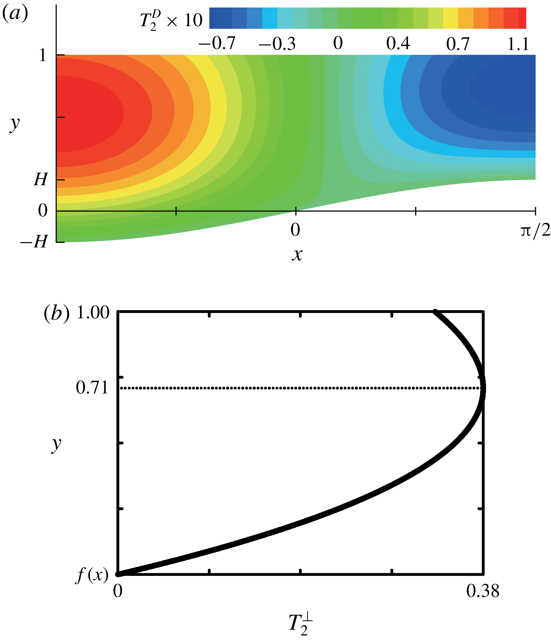
A typical contour plot of $T_{2}^{D}$ is shown in figure 7(a). At a specified $x$ , $T_{2}^{\bot }$ causes $T_{2}^{D}$ to change cubically along the vertical direction and the maximum $|T_{2}^{D}|$ to be located underneath the interface, as plotted in figure 7(b). Along the horizontal direction, the normalised substrate ‘curvature’ affects $T_{2}^{D}$ , as indicated by $\unicode[STIX]{x1D719}_{0,xx}(x)$ .

The corresponding interfacial $T_{2}^{D}$ profile becomes

(3.39)

$$\begin{eqnarray}\displaystyle T_{2}^{D}(x,1) & = & \displaystyle \unicode[STIX]{x1D719}_{0,xx}(x)T_{2}^{\bot }(x,1)\nonumber\\ \displaystyle & {\approx} & \displaystyle \frac{3+\mathit{Bi}}{12(1+\mathit{Bi})^{2}}\hat{f}^{\prime \prime }(x)+\frac{1}{2(1+\mathit{Bi})^{3}}\left(\frac{\mathit{Bi}(3+\mathit{Bi})}{3}\hat{f}^{\prime 2}(x)-\hat{f}(x)\hat{f}^{\prime \prime }(x)\right)\!H.\qquad\end{eqnarray}$$

$\hat{f}^{\prime \prime }(x)$ in the first term of (3.39) indicates that $T_{2}^{D}(x,1)$ may decrease in $C_{0}$ . To check whether $T_{2}^{D}(x,1)$ decreases or not, one needs to examine the sign of the interfacial $T_{2}^{D}$ gradient.

Figure 7.

(a) Contour plot of $T_{2}^{D}$ and (b) the plot of $T_{2}^{\bot }$ at $x=0$ . $\mathit{Bi}=1$ and $H=0.2$ for all plots.

The interfacial $T_{2}^{D}$ gradient, $T_{2,x}^{D}|_{y=1}$ , becomes

(3.40)

$$\begin{eqnarray}\unicode[STIX]{x1D6E9}_{2}^{iD}(x)\approx \left(\frac{3+\mathit{Bi}}{12(1+\mathit{Bi})^{2}}+\frac{\mathit{Bi}^{2}+3\mathit{Bi}-3}{3(1+\mathit{Bi})^{3}}\hat{f}(x)H\right)\hat{f}^{\prime \prime \prime }(x).\end{eqnarray}$$

The relationships $\hat{f}^{\prime \prime \prime }(x)=-\hat{f}^{\prime }(x)$ and $\hat{f}^{\prime \prime }(x)=-\hat{f}(x)$ for the sinusoidal topography are used in (3.40). The $\unicode[STIX]{x1D6E9}_{2}^{iD}(x)$ profile directly depends on $\hat{f}^{\prime \prime \prime }(x)$ , which is equal to $-\hat{f}^{\prime }(x)=-\text{cos}\,x$ in this study. The term inside the parentheses becomes positive when

(3.41)

$$\begin{eqnarray}H<\frac{(\mathit{Bi}^{2}+4\mathit{Bi}+3)}{4(\mathit{Bi}^{2}+3\mathit{Bi}-3)}.\end{eqnarray}$$

Under this condition, which is considered in this section, $\hat{f}^{\prime \prime \prime }(x)$ solely determines the sign of $\unicode[STIX]{x1D6E9}_{2}^{iD}(x)$ , and thus $\unicode[STIX]{x1D6E9}_{2}^{iD}(x)$ is always negative in $C_{0}$ . The sign of $\unicode[STIX]{x1D6E9}_{2}^{iD}(x)$ is opposite to that of $\unicode[STIX]{x1D6E9}_{0}^{i}(x)$ , which is proportional to $f^{\prime }(x)$ , as shown in (3.18a ). Note that $\hat{f}^{\prime \prime \prime }(x)$ comes from the horizontal diffusion of $T_{0}$ . For $\mathit{Bi}=1$ , any $0<H<1$ satisfies the condition in (3.41). For any $\mathit{Bi}$ , $0<H\leqslant 0.25$ satisfies the condition in (3.41). The other cases not satisfying (3.41) will be discussed in § 5.

The solution for $T_{2}^{C}$ is

(3.42)

$$\begin{eqnarray}T_{2}^{C}(x,y)=Q_{2}(x,y)+\tilde{a}_{2}(x)y+\tilde{b}_{2}(x),\end{eqnarray}$$

where

(3.43)

$$\begin{eqnarray}Q_{2}(x,y)=\int ^{\unicode[STIX]{x1D709}}\int ^{\unicode[STIX]{x1D709}}q_{2}(x,\unicode[STIX]{x1D709})\,\text{d}\unicode[STIX]{x1D709}\,\text{d}\unicode[STIX]{x1D709}.\end{eqnarray}$$

Here, we have introduced an integral notation $\int ^{\unicode[STIX]{x1D709}}g(x,\unicode[STIX]{x1D709})\,\text{d}\unicode[STIX]{x1D709}$ . The indefinite integral of $g(x,y)$ over $y$ can be written as follows:

(3.44)

$$\begin{eqnarray}\int g(x,y)\,\text{d}y=\int ^{\unicode[STIX]{x1D709}}g(x,\unicode[STIX]{x1D709})\,\text{d}\unicode[STIX]{x1D709}+\unicode[STIX]{x1D6FC}(x),\end{eqnarray}$$

where $\unicode[STIX]{x1D6FC}(x)$ is an arbitrary function of $x$ . The notation represents the indefinite integral with $\unicode[STIX]{x1D6FC}(x)=0$ . $Q_{2}(x,y)$ , $\tilde{a}_{2}(x)$ and $\tilde{b}_{2}(x)$ are given by (A 1)–(A 7).

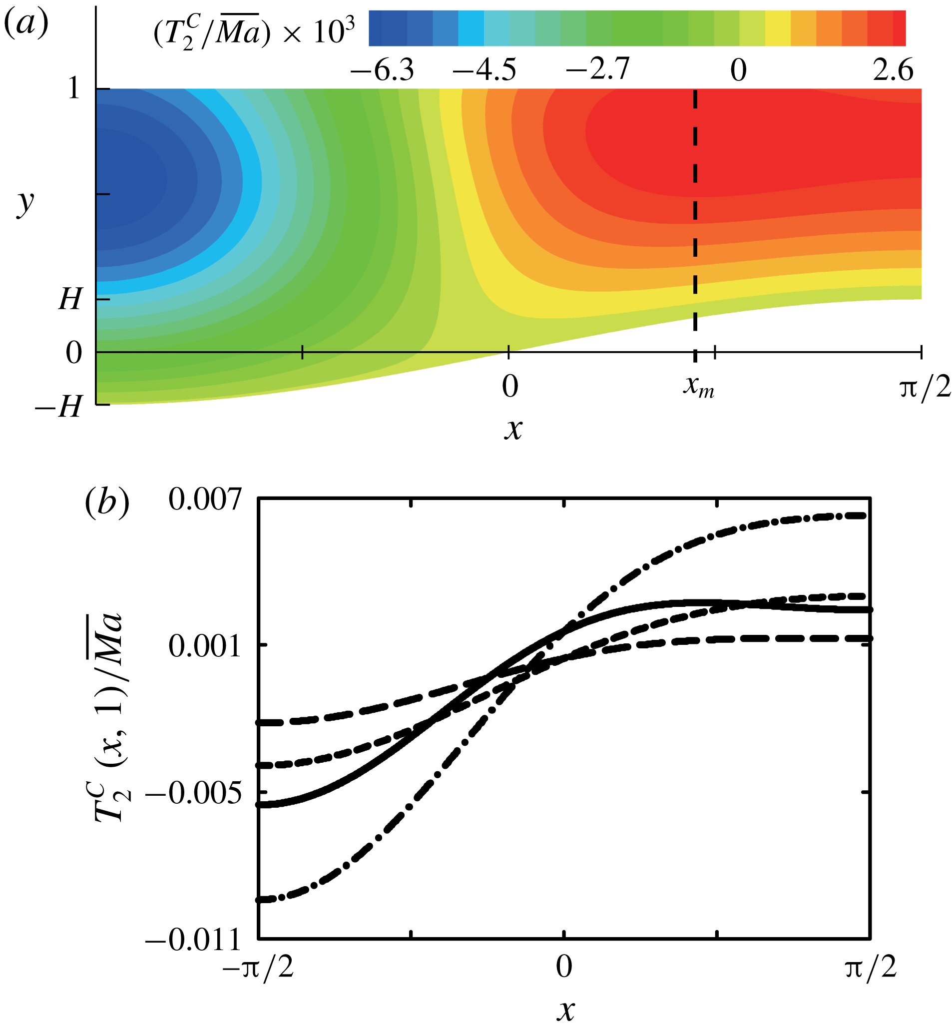
$T_{2}^{C}$ is generated inside the liquid layer by the source term $q_{2}$ . The magnitude of $T_{2}^{C}$ is directly proportional to $\overline{\mathit{Ma}}$ because of the source term. Therefore, we examine the normalised $T_{2}^{C}/\overline{\mathit{Ma}}$ for simplicity to describe $T_{2}^{C}$ . Figure 8(a) presents a contour plot of $T_{2}^{C}/\overline{\mathit{Ma}}$ for $\mathit{Bi}=1$ and $H=0.2$ . The $T_{2}^{C}$ contour plot is dramatically different from $T_{0}$ ; the vertical $T_{2}^{C}$ gradient is not uniform along $y$ , and the $T_{2}^{C}$ profile does not follow the substrate shape. Among these differences, the interfacial $T_{2}^{C}$ profile needs to be examined in detail, because it is likely to significantly contribute to the second correction for the flows via generating the interfacial $\unicode[STIX]{x1D714}_{2}$ . $T_{0}(x,1)$ increases monotonically along the $x$ direction in $C_{0}$ , whereas $T_{2}^{C}(x,1)$ changes non-monotonically; the minimum value appears at $x=-\unicode[STIX]{x03C0}/2$ , but the maximum value is located at $x=x_{m}<\unicode[STIX]{x03C0}/2$ in $C_{0}$ , as shown in figure 8(b).

Figure 8.

(a) Contour plot of $T_{2}^{C}/\overline{\mathit{Ma}}$ for $\mathit{Bi}=1$ and $H=0.2$ , and (b) $T_{2}^{C}(x,1)/\overline{\mathit{Ma}}$ profile corresponding to $x$ : ——, $\mathit{Bi}=1$ , $H=0.2$ ; — — —, $\mathit{Bi}=2$ , $H=0.2$ ; – ⋅ – ⋅ –, $\mathit{Bi}=1$ , $H=0.1$ ; – – – –, $\mathit{Bi}=2$ , $H=0.1$ .

Consequently, the interfacial $T_{2}^{C}$ gradient, $T_{2,x}^{C}|_{y=1}=\unicode[STIX]{x1D6E9}_{2}^{iC}(x)$ , changes from positive to negative across $x=x_{m}$ in $C_{0}$ for $Bi=1$ and $H=0.2$ . Here, we divide the interface into two regions: $-\unicode[STIX]{x03C0}/2<x<x_{m}$ ( $\unicode[STIX]{x1D6E9}_{2}^{iC}>0$ ), which shows a steep interfacial $T_{2}^{C}$ gradient, and $x_{m}<x<\unicode[STIX]{x03C0}/2$ ( $\unicode[STIX]{x1D6E9}_{2}^{iC}<0$ ), which exhibits a marginally decreasing $T_{2}^{C}(x,1)$ profile. However, the non-monotonicity in $T_{2}^{C}(x,1)$ vanishes, as $Bi$ increases or $H$ decreases. See figure 8(b). As $\mathit{Bi}$ or $H$ increases, the minimum value of $T_{2}^{C}(x,1)$ increases and the maximum decreases, and then the magnitude of $\unicode[STIX]{x1D6E9}_{2}^{iC}$ decreases.

To summarise, $A^{2}T_{2}=A^{2}(T_{2}^{D}+T_{2}^{C})$ is the second correction for the temperature field. The horizontal diffusion and the convection of $T_{0}$ cause $A^{2}T_{2}^{D}$ and $A^{2}T_{2}^{C}$ , respectively. When figures 7(a) and 8(a) are compared with figure 3(a), in general, the horizontal diffusion of heat weakens the interfacial temperature gradient, and the convection of heat intensifies it. The interfacial $T_{2}$ gradient directly affects the second correction for the flows, which will be discussed in the next section.

3.2.2 Flow field

To the second correction, $\unicode[STIX]{x1D714}_{2}$ and $\unicode[STIX]{x1D713}_{2}$ satisfy the governing equations

(3.45)

$$\begin{eqnarray}\displaystyle & \unicode[STIX]{x1D714}_{2,yy}=-\unicode[STIX]{x1D714}_{0,xx}+\underbrace{\overline{\mathit{Re}}(\unicode[STIX]{x1D713}_{0,y}\unicode[STIX]{x1D714}_{0,x}-\unicode[STIX]{x1D713}_{0,x}\unicode[STIX]{x1D714}_{0,y})}_{=s_{2}(x,y)}, & \displaystyle\end{eqnarray}$$

(3.46)

$$\begin{eqnarray}\displaystyle & \unicode[STIX]{x1D714}_{2}=-\unicode[STIX]{x1D713}_{2,yy}-\unicode[STIX]{x1D713}_{0,xx}, & \displaystyle\end{eqnarray}$$

together with the boundary conditions

(3.47)

$$\begin{eqnarray}\displaystyle & \unicode[STIX]{x1D714}_{2}=T_{2,x},\quad \text{on}~y=1, & \displaystyle\end{eqnarray}$$

(3.48)

$$\begin{eqnarray}\displaystyle & \unicode[STIX]{x1D713}_{2}=\unicode[STIX]{x1D713}_{2,y}=0,\quad \text{on}~y=f(x), & \displaystyle\end{eqnarray}$$

where $\unicode[STIX]{x1D714}_{2}|_{y=1}=-u_{2,y}|_{y=1}$ in (3.47), and the condition of no net mass flow

(3.49)

$$\begin{eqnarray}\unicode[STIX]{x1D713}_{2}=0,\quad \text{on}~y=1.\end{eqnarray}$$

$-\unicode[STIX]{x1D714}_{0,xx}$ is the term derived from the horizontal diffusion of $\unicode[STIX]{x1D714}_{0}$ , and $s_{2}$ is the term derived from the convection of $\unicode[STIX]{x1D714}_{0}$ under the flows in the leading order.

The solutions satisfying the above set of equations can be split into homogeneous and particular parts, i.e. $\unicode[STIX]{x1D714}_{2}=\unicode[STIX]{x1D714}_{2}^{h}+\unicode[STIX]{x1D714}_{2}^{p}$ , $u_{2}=u_{2}^{h}+u_{2}^{p}$ and $\unicode[STIX]{x1D713}_{2}=\unicode[STIX]{x1D713}_{2}^{h}+\unicode[STIX]{x1D713}_{2}^{p}$ , where the superscript $h$ denotes the corresponding quantities in the homogeneous part, and $p$ indicates those in the particular part. The problems for the homogeneous part are

(3.50)

$$\begin{eqnarray}\displaystyle & \unicode[STIX]{x1D714}_{2,yy}^{h}=0, & \displaystyle\end{eqnarray}$$

(3.51)

$$\begin{eqnarray}\displaystyle & \unicode[STIX]{x1D714}_{2}^{h}=-\unicode[STIX]{x1D713}_{2,yy}^{h}, & \displaystyle\end{eqnarray}$$

(3.52)

$$\begin{eqnarray}\displaystyle & \unicode[STIX]{x1D714}_{2}^{h}=T_{2,x},\quad \text{on}~y=1, & \displaystyle\end{eqnarray}$$

(3.53)

$$\begin{eqnarray}\displaystyle & \unicode[STIX]{x1D713}_{2}^{h}=\unicode[STIX]{x1D713}_{2,y}^{h}=0,\quad \text{on}~y=f(x), & \displaystyle\end{eqnarray}$$

(3.54)

$$\begin{eqnarray}\displaystyle & \unicode[STIX]{x1D713}_{2}^{h}=0,\quad \text{on}~y=1, & \displaystyle\end{eqnarray}$$

and the problems for the particular part are

(3.55)

$$\begin{eqnarray}\displaystyle & \unicode[STIX]{x1D714}_{2,yy}^{p}=-\unicode[STIX]{x1D714}_{0,xx}+s_{2}, & \displaystyle\end{eqnarray}$$

(3.56)

$$\begin{eqnarray}\displaystyle & \unicode[STIX]{x1D714}_{2}^{p}=-\unicode[STIX]{x1D713}_{2,yy}^{p}-\unicode[STIX]{x1D713}_{0,xx}, & \displaystyle\end{eqnarray}$$

(3.57)

$$\begin{eqnarray}\displaystyle & \unicode[STIX]{x1D714}_{2}^{p}=0,\quad \text{on}~y=1, & \displaystyle\end{eqnarray}$$

(3.58)

$$\begin{eqnarray}\displaystyle & \unicode[STIX]{x1D713}_{2}^{p}=\unicode[STIX]{x1D713}_{2,y}^{p}=0,\quad \text{on}~y=f(x), & \displaystyle\end{eqnarray}$$

(3.59)

$$\begin{eqnarray}\displaystyle & \unicode[STIX]{x1D713}_{2}^{p}=0,\quad \text{on}~y=1. & \displaystyle\end{eqnarray}$$

The interfacial $T_{2}$ gradient, $T_{2,x}|_{y=1}=\unicode[STIX]{x1D6E9}_{2}^{i}(x)$ , is responsible for the generation of $\unicode[STIX]{x1D714}_{2}^{h}$ on the interface, as described by (3.52), and $\unicode[STIX]{x1D714}_{2}^{h}$ diffuses vertically. In the particular part, there are two source terms, $-\unicode[STIX]{x1D714}_{0,xx}$ and $s_{2}$ , as described by (3.55). $\unicode[STIX]{x1D714}_{2}^{p}$ also propagates vertically.

The homogeneous solutions are

(3.60)

$$\begin{eqnarray}\displaystyle \unicode[STIX]{x1D714}_{2}^{h}(x,Y) & = & \displaystyle \unicode[STIX]{x1D6E9}_{2}^{i}(x)\bar{\unicode[STIX]{x1D714}}_{0}(Y)\nonumber\\ \displaystyle & = & \displaystyle \underbrace{\unicode[STIX]{x1D6E9}_{2}^{iD}(x)\bar{\unicode[STIX]{x1D714}}_{0}(Y)}_{=\unicode[STIX]{x1D714}_{2}^{hD}(x,Y)}+\underbrace{\unicode[STIX]{x1D6E9}_{2}^{iC}(x)\bar{\unicode[STIX]{x1D714}}_{0}(Y)}_{=\unicode[STIX]{x1D714}_{2}^{hC}(x,Y)},\end{eqnarray}$$

(3.61)

$$\begin{eqnarray}\displaystyle u_{2}^{h}(x,Y) & = & \displaystyle \unicode[STIX]{x1D6E9}_{2}^{i}(x)D(x)\bar{u}_{0}(Y)\nonumber\\ \displaystyle & = & \displaystyle \underbrace{\unicode[STIX]{x1D6E9}_{2}^{iD}(x)D(x)\bar{u}_{0}(Y)}_{=u_{2}^{hD}(x,Y)}+\underbrace{\unicode[STIX]{x1D6E9}_{2}^{iC}(x)D(x)\bar{u}_{0}(Y)}_{=u_{2}^{hC}(x,Y)},\end{eqnarray}$$

(3.62)

$$\begin{eqnarray}\displaystyle \unicode[STIX]{x1D713}_{2}^{h}(x,Y) & = & \displaystyle \unicode[STIX]{x1D6E9}_{2}^{i}(x)D^{2}(x)\bar{\unicode[STIX]{x1D713}}_{0}(Y)\nonumber\\ \displaystyle & = & \displaystyle \underbrace{\unicode[STIX]{x1D6E9}_{2}^{iD}(x)D^{2}(x)\bar{\unicode[STIX]{x1D713}}_{0}(Y)}_{=\unicode[STIX]{x1D713}_{2}^{hD}(x,Y)}+\underbrace{\unicode[STIX]{x1D6E9}_{2}^{iC}(x)D^{2}(x)\bar{\unicode[STIX]{x1D713}}_{0}(Y)}_{=\unicode[STIX]{x1D713}_{2}^{hC}(x,Y)}.\end{eqnarray}$$

This function splitting in (3.60)–(3.62) naturally appears because the governing equations are similar to those in the basic solutions. Unlike $\unicode[STIX]{x1D714}_{0}$ , however, the interfacial $\unicode[STIX]{x1D714}_{2}^{h}$ is generated by $\unicode[STIX]{x1D6E9}_{2}^{i}(x)=\unicode[STIX]{x1D6E9}_{2}^{iD}(x)+\unicode[STIX]{x1D6E9}_{2}^{iC}(x)$ . The homogeneous solutions are the linear combinations of two parts: $\unicode[STIX]{x1D714}_{2}^{h}=\unicode[STIX]{x1D714}_{2}^{hD}+\unicode[STIX]{x1D714}_{2}^{hC}$ , $u_{2}^{h}=u_{2}^{hD}+u_{2}^{hC}$ and $\unicode[STIX]{x1D713}_{2}^{h}=\unicode[STIX]{x1D713}_{2}^{hD}+\unicode[STIX]{x1D713}_{2}^{hC}$ , where superscripts $hD$ and $hC$ denote that the corresponding quantities concern $\unicode[STIX]{x1D6E9}_{2}^{iD}(x)$ and $\unicode[STIX]{x1D6E9}_{2}^{iC}(x)$ , respectively.

Figure 9.

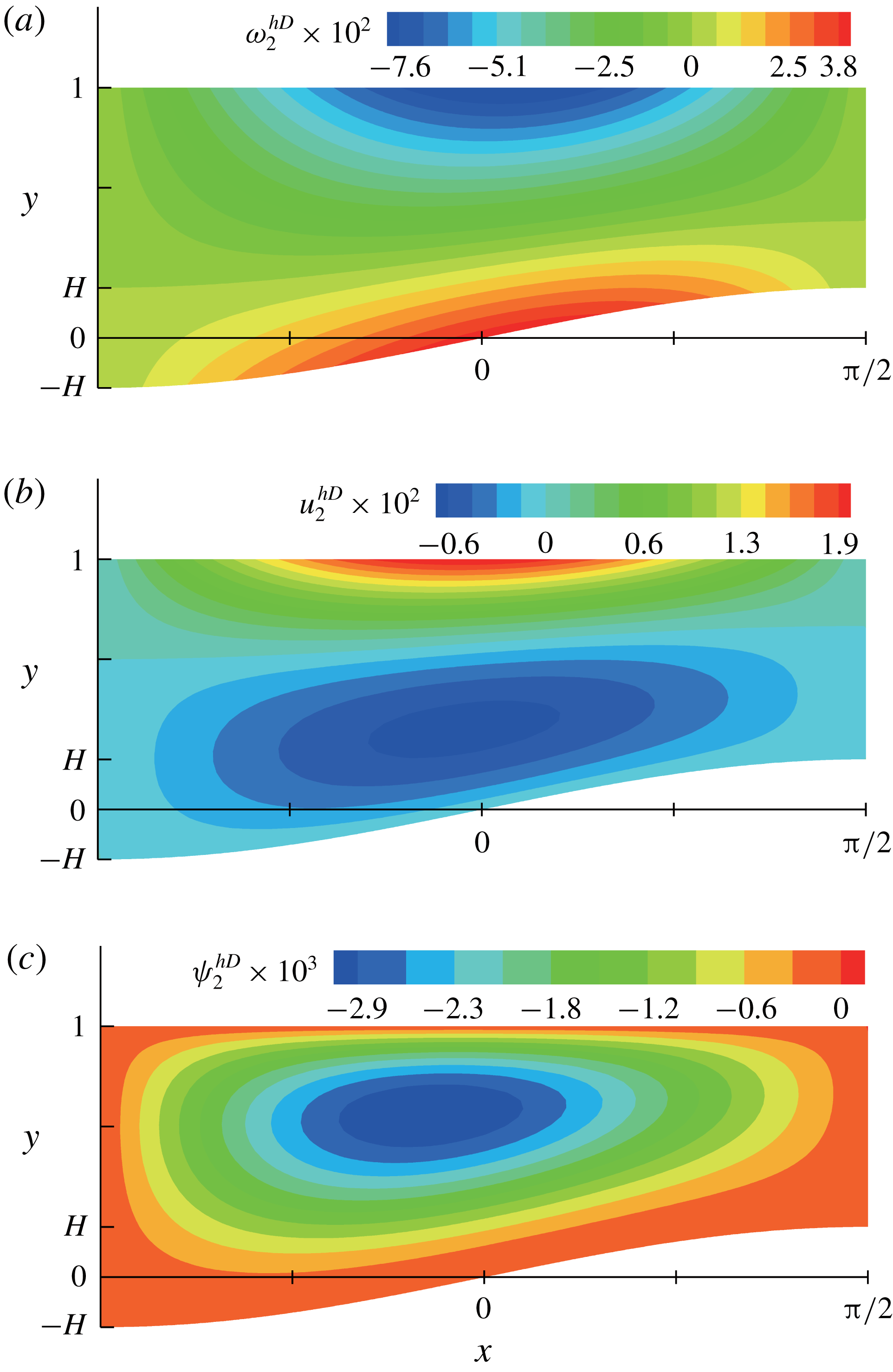
Contour plots of (a) $\unicode[STIX]{x1D714}_{2}^{hD}$ , (b) $u_{2}^{hD}$ and (c) $\unicode[STIX]{x1D713}_{2}^{hD}$ for $\mathit{Bi}=1$ and $H=0.2$ .

The interfacial $\unicode[STIX]{x1D714}_{2}^{hD}$ is generated by $\unicode[STIX]{x1D6E9}_{2}^{iD}(x)$ and diffuses throughout the layer vertically, as described by $\bar{\unicode[STIX]{x1D714}}_{0}(Y)$ . $\unicode[STIX]{x1D6E9}_{2}^{iD}(x)$ is the driving force for $\unicode[STIX]{x1D714}_{2}^{hD}$ , $u_{2}^{hD}$ and $\unicode[STIX]{x1D713}_{2}^{hD}$ , and (3.40) indicates that $\unicode[STIX]{x1D6E9}_{2}^{iD}(x)$ has the sign opposite to that of $\unicode[STIX]{x1D6E9}_{0}^{i}(x)$ . Therefore, the direction of recirculation, as shown in figure 9, is opposite to that in the basic solutions, as shown in figure 5.

The interfacial $\unicode[STIX]{x1D714}_{2}^{hC}$ is generated by $\unicode[STIX]{x1D6E9}_{2}^{iC}(x)$ , and it diffuses vertically again. $\unicode[STIX]{x1D6E9}_{2}^{iC}(x)$ is the driving force for $\unicode[STIX]{x1D714}_{2}^{hC}$ , $u_{2}^{hC}$ and $\unicode[STIX]{x1D713}_{2}^{hC}$ . The linear dependence of $T_{2}^{C}$ on $\overline{\mathit{Ma}}$ is transferred to the solutions via $\unicode[STIX]{x1D6E9}_{2}^{iC}(x)$ . 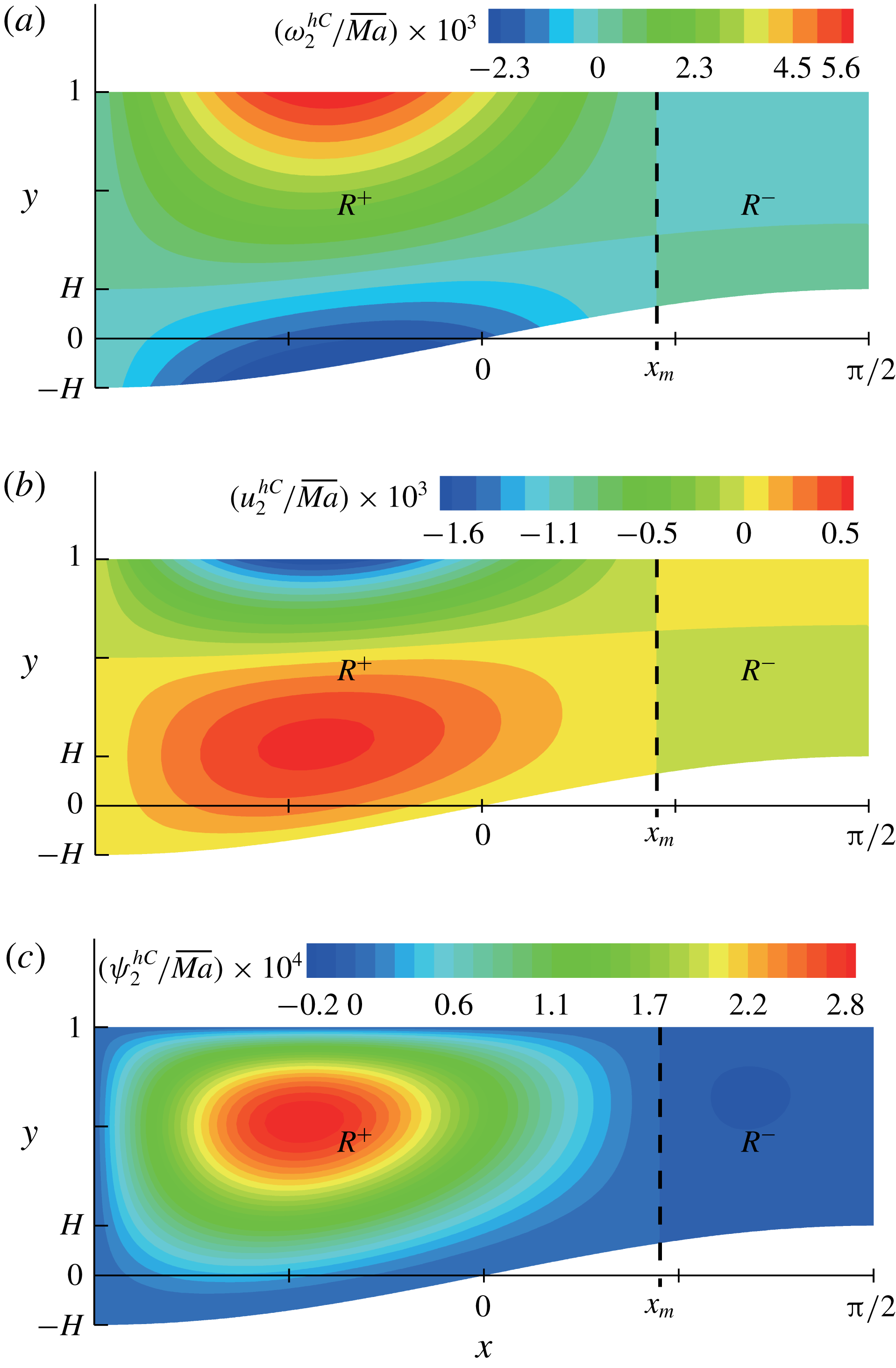Figure 10 presents the contour plots of $\unicode[STIX]{x1D714}_{2}^{hC}/\overline{\mathit{Ma}}$ , $u_{2}^{hC}/\overline{\mathit{Ma}}$ and $\unicode[STIX]{x1D713}_{2}^{hC}/\overline{\mathit{Ma}}$ for $\mathit{Bi}=1$ and $H=0.2$ . The non-monotonic $T_{2}^{C}(x,1)$ profile leads to the anticlockwise recirculation for $R^{+}$ region ( $-\unicode[STIX]{x03C0}/2<x<x_{m}$ ) and the clockwise recirculation for $R^{-}$ region ( $x_{m}<x<\unicode[STIX]{x03C0}/2$ ), and the recirculation is stronger inside $R^{+}$ than that inside $R^{-}$ , as the sign and the magnitude of the driving force $\unicode[STIX]{x1D6E9}_{2}^{iC}(x)$ are transferred inside via the vertical diffusion. Additionally, the vertical diffusion clearly explains why the boundary between $R^{+}$ and $R^{-}$ is a straight line, i.e. $x=x_{m}$ in figure 10. When $Bi$ increases or $H$ decreases, positive $\unicode[STIX]{x1D6E9}_{2}^{iC}$ along the entire interface causes only the anticlockwise recirculation in $C_{0}$ , which implies the $R^{-}$ region disappears.

Figure 10.

Contour plots of (a) $\unicode[STIX]{x1D714}_{2}^{hC}/\overline{\mathit{Ma}}$ , (b) $u_{2}^{hC}/\overline{\mathit{Ma}}$ and (c) $\unicode[STIX]{x1D713}_{2}^{hC}/\overline{\mathit{Ma}}$ for $\mathit{Bi}=1$ and $H=0.2$ .

The particular solutions are also the linear combinations of two parts: $\unicode[STIX]{x1D714}_{2}^{p}=-(\unicode[STIX]{x1D713}_{2,yy}^{pD}+\unicode[STIX]{x1D713}_{0,xx})-\unicode[STIX]{x1D713}_{2,yy}^{pC}$ , $u_{2}^{p}=u_{2}^{pD}+u_{2}^{pC}$ and $\unicode[STIX]{x1D713}_{2}^{p}=\unicode[STIX]{x1D713}_{2}^{pD}+\unicode[STIX]{x1D713}_{2}^{pC}$ , where the superscripts $pD$ and $pC$ denote that the corresponding quantities arise from the source terms $-\unicode[STIX]{x1D714}_{0,xx}$ and $s_{2}$ , respectively. Unlike the homogeneous solutions, $\unicode[STIX]{x1D714}_{2}^{p}$ , $u_{2}^{p}$ and $\unicode[STIX]{x1D713}_{2}^{p}$ are generated inside the liquid layer by the source terms. They are

(3.63)

$$\begin{eqnarray}\displaystyle \unicode[STIX]{x1D714}_{2}^{p}(x,y) & = & \displaystyle \underbrace{Z_{2,yy}(x,y)-\tilde{c}_{2}^{\,pD}(x)y-\tilde{d}_{2}^{pD}(x)}_{=-\unicode[STIX]{x1D713}_{2,yy}^{pD}(x,y)}-\unicode[STIX]{x1D713}_{0,xx}(x,y)\nonumber\\ \displaystyle & & \displaystyle +\,\underbrace{S_{2,yy}(x,y)-\tilde{c}_{2}^{\,pC}(x)y-\tilde{d}_{2}^{pC}(x)}_{=-\unicode[STIX]{x1D713}_{2,yy}^{pC}(x,y)},\end{eqnarray}$$

(3.64)

$$\begin{eqnarray}\displaystyle u_{2}^{p}(x,y) & = & \displaystyle \underbrace{-Z_{2,y}(x,y)+\frac{\tilde{c}_{2}^{\,pD}(x)}{2}y^{2}+\tilde{d}_{2}^{pD}(x)y+\tilde{e}_{2}^{pD}(x)}_{=u_{2}^{pD}(x,y)}\nonumber\\ \displaystyle & & \displaystyle \underbrace{-S_{2,y}(x,y)+\frac{\tilde{c}_{2}^{\,pC}(x)}{2}y^{2}+\tilde{d}_{2}^{pC}(x)y+\tilde{e}_{2}^{pC}(x)}_{=u_{2}^{pC}(x,y)},\end{eqnarray}$$

(3.65)

$$\begin{eqnarray}\displaystyle \unicode[STIX]{x1D713}_{2}^{p}(x,y) & = & \displaystyle \underbrace{-Z_{2}(x,y)+\frac{\tilde{c}_{2}^{\,pD}(x)}{6}y^{3}+\frac{\tilde{d}_{2}^{pD}(x)}{2}y^{2}+\tilde{e}_{2}^{pD}(x)y+\tilde{f}_{2}^{pD}(x)}_{=\unicode[STIX]{x1D713}_{2}^{pD}(x,y)}\nonumber\\ \displaystyle & & \displaystyle \underbrace{-S_{2}(x,y)+\frac{\tilde{c}_{2}^{\,pC}(x)}{6}y^{3}+\frac{\tilde{d}_{2}^{pC}(x)}{2}y^{2}+\tilde{e}_{2}^{pC}(x)y+\tilde{f}_{2}^{pC}(x)}_{=\unicode[STIX]{x1D713}_{2}^{pC}(x,y)},\end{eqnarray}$$

where

(3.66)

$$\begin{eqnarray}\displaystyle & \displaystyle Z_{2}(x,y)=\int ^{\unicode[STIX]{x1D709}}\int ^{\unicode[STIX]{x1D709}}\int ^{\unicode[STIX]{x1D709}}\int ^{\unicode[STIX]{x1D709}}(-\unicode[STIX]{x1D714}_{0,xx}(x,\unicode[STIX]{x1D709})+\unicode[STIX]{x1D713}_{0,xx\unicode[STIX]{x1D709}\unicode[STIX]{x1D709}}(x,\unicode[STIX]{x1D709}))\,\text{d}\unicode[STIX]{x1D709}\,\text{d}\unicode[STIX]{x1D709}\,\text{d}\unicode[STIX]{x1D709}\,\text{d}\unicode[STIX]{x1D709}, & \displaystyle\end{eqnarray}$$

(3.67)

$$\begin{eqnarray}\displaystyle & \displaystyle S_{2}(x,y)=\int ^{\unicode[STIX]{x1D709}}\int ^{\unicode[STIX]{x1D709}}\int ^{\unicode[STIX]{x1D709}}\int ^{\unicode[STIX]{x1D709}}s_{2}(x,\unicode[STIX]{x1D709})\,\text{d}\unicode[STIX]{x1D709}\,\text{d}\unicode[STIX]{x1D709}\,\text{d}\unicode[STIX]{x1D709}\,\text{d}\unicode[STIX]{x1D709}. & \displaystyle\end{eqnarray}$$

$Z_{2}(x,y),S_{2}(x,y)$ , $\tilde{c}_{2}^{\,pD}(x)$ , $\tilde{c}_{2}^{\,pC}(x)$ , $\tilde{d}_{2}^{pD}(x)$ , $\tilde{d}_{2}^{pC}(x)$ , $\tilde{e}_{2}^{pD}(x)$ , $\tilde{e}_{2}^{pC}(x)$ , $\tilde{f}_{2}^{pD}(x)$ , $\tilde{f}_{2}^{pC}(x)$ and $\unicode[STIX]{x1D713}_{0,xx}(x,y)$ are given by (A 8)–(A 26).

Figure 11.

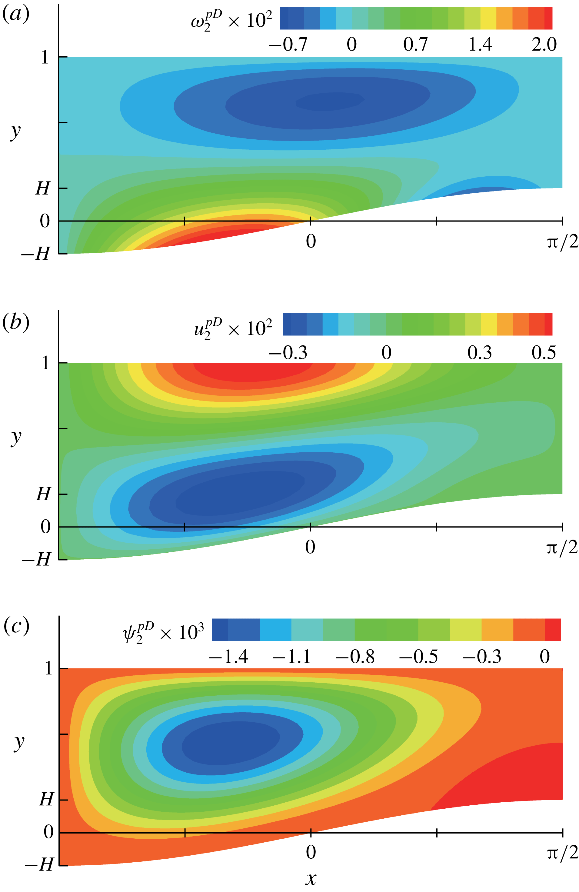
Contour plots of (a) $\unicode[STIX]{x1D714}_{2}^{pD}$ , (b) $u_{2}^{pD}$ and (c) $\unicode[STIX]{x1D713}_{2}^{pD}$ for $\mathit{Bi}=1$ and $H=0.2$ .

Figure 11 shows $\unicode[STIX]{x1D714}_{2}^{pD}=-(\unicode[STIX]{x1D713}_{2,yy}^{pD}+\unicode[STIX]{x1D713}_{0,xx}),u_{2}^{pD}$ and $\unicode[STIX]{x1D713}_{2}^{pD}$ for $\mathit{Bi}=1$ and $H=0.2$ . They behave similarly to $\unicode[STIX]{x1D714}_{2}^{hD}$ , $u_{2}^{hD}$ and $\unicode[STIX]{x1D713}_{2}^{hD}$ in figure 9, which implies both the quantities with superscripts $hD$ and $pD$ cause the recirculation counter-rotation to the vortex in the basic solutions and weaken the overall flow. The similarity probably arises from the common term $\unicode[STIX]{x1D719}_{0,xxx}(x)$ . For the quantities with $hD$ , $\unicode[STIX]{x1D719}_{0}(x)$ in $T_{0}$ is differentiated two times with respect to $x$ via the horizontal diffusion of $T_{0}$ for $T_{2}^{D}$ and once again via obtaining interfacial $T_{2}^{D}$ gradient. For the quantities with $pD$ , $\unicode[STIX]{x1D719}_{0}(x)$ in $T_{0}$ is differentiated once with respect to $x$ via obtaining interfacial $T_{0}$ gradient for $\unicode[STIX]{x1D714}_{0}$ and two times again via the horizontal diffusion of $\unicode[STIX]{x1D714}_{0}$ . Therefore, $\unicode[STIX]{x1D719}_{0,xxx}(x)$ naturally appears in all the quantities. However, the magnitudes of the quantities with $pD$ are smaller than those of the quantities with $hD$ . One can understand $\unicode[STIX]{x1D714}_{2}^{pD}$ , $u_{2}^{pD}$ and $\unicode[STIX]{x1D713}_{2}^{pD}$ make a minor contribution to weakening the overall flow, whereas the quantities with $hD$ make the major contribution.

With the parameter set of $\mathit{Bi}=1$ and $H=0.2$ , the maximum values of $|-\unicode[STIX]{x1D713}_{2,yy}^{pC}|$ , $|u_{2}^{pC}|$ and $|\unicode[STIX]{x1D713}_{2}^{pC}|$ are estimated to be $1.89\overline{\mathit{Re}}\times 10^{-4}$ , $5.29\overline{\mathit{Re}}\times 10^{-5}$ and $1.37\overline{\mathit{Re}}\times 10^{-5}$ , respectively. This implies that the contributions of the source term $s_{2}$ are not significant in the second-order solutions for a typical fluid, of which $\mathit{Pr}$ is generally $O(1)$ or higher.

To summarise, $A^{2}\unicode[STIX]{x1D714}_{2}=A^{2}(\unicode[STIX]{x1D714}_{2}^{hD}+\unicode[STIX]{x1D714}_{2}^{hC}+\unicode[STIX]{x1D714}_{2}^{pD}+\unicode[STIX]{x1D714}_{2}^{pC})$ is the second correction for the flows. The horizontal diffusion and the convection of $T_{0}$ cause $A^{2}\unicode[STIX]{x1D6E9}_{2}^{iD}(x)$ and $A^{2}\unicode[STIX]{x1D6E9}_{2}^{iC}(x)$ , and they are responsible for the behaviours of $A^{2}\unicode[STIX]{x1D714}_{2}^{hD}$ and $A^{2}\unicode[STIX]{x1D714}_{2}^{hC}$ as the driving forces, respectively. When figures 9 and 10 are compared with figure 5, in general, the horizontal diffusion of heat weakens and the convection of heat intensifies the overall flow. In addition, the horizontal diffusion of $\unicode[STIX]{x1D714}_{0}$ affects $A^{2}\unicode[STIX]{x1D714}_{2}^{pD}$ , which makes a minor contribution to weakening the overall flow, and the convection of $\unicode[STIX]{x1D714}_{0}$ induces $A^{2}\unicode[STIX]{x1D714}_{2}^{pC}$ , which is insignificant in the second-order solution under the conditions used in this study.

3.3 Interfacial vorticity

The vertical diffusion of the interfacial vorticity mainly governs the thermocapillary flows in this study. Therefore, the magnitude of the interfacial vorticity can be a representative quantity for the intensity of the flows. The contributions from the convection and the diffusion to the flows can be indirectly measured by the amount of interfacial vorticity from them.

The vorticity is represented by the second-order solution

(3.68)

$$\begin{eqnarray}\unicode[STIX]{x1D714}=\unicode[STIX]{x1D714}_{0}+A^{2}(\unicode[STIX]{x1D714}_{2}^{hD}+\unicode[STIX]{x1D714}_{2}^{hC}+\unicode[STIX]{x1D714}_{2}^{pD}+\unicode[STIX]{x1D714}_{2}^{pC})+O(A^{3}).\end{eqnarray}$$

According to our analysis, the vertical diffusion of the interfacial vorticity in the leading order is the dominant factor in generating the flows. Therefore, the intensity of the flows can be characterised by the interfacial $\unicode[STIX]{x1D714}_{0}$

(3.69)

$$\begin{eqnarray}\unicode[STIX]{x1D714}_{0}(x,1)=\unicode[STIX]{x1D6E9}_{0}^{i}(x).\end{eqnarray}$$

The magnitude of $\unicode[STIX]{x1D6E9}_{0}^{i}(x)$ can be approximated by $(\unicode[STIX]{x1D6FF}T_{0}|_{y=1})/\unicode[STIX]{x1D6FF}x$ , where $\unicode[STIX]{x1D6FF}T|_{y=1}=T(\unicode[STIX]{x03C0}/2,1)-T(-\unicode[STIX]{x03C0}/2,1)$ in $C_{0}$ , and $\unicode[STIX]{x1D6FF}x=\unicode[STIX]{x03C0}$ is the horizontal size of the unit cell. Using (3.13), $(\unicode[STIX]{x1D6FF}T_{0}|_{y=1})/\unicode[STIX]{x1D6FF}x$ is given by

(3.70)

$$\begin{eqnarray}\frac{\unicode[STIX]{x1D6FF}T_{0}|_{y=1}}{\unicode[STIX]{x1D6FF}x}=\frac{1+\mathit{Bi}}{\unicode[STIX]{x03C0}[(1+\mathit{Bi})^{2}-Bi^{2}H^{2}]}.\end{eqnarray}$$

In the second correction, $A^{2}\unicode[STIX]{x1D714}_{2}^{hD}$ and $A^{2}\unicode[STIX]{x1D714}_{2}^{hC}$ are caused by the vertical diffusion of the interfacial $A^{2}\unicode[STIX]{x1D714}_{2}$ , whereas $A^{2}\unicode[STIX]{x1D714}_{2}^{pD}$ and $A^{2}\unicode[STIX]{x1D714}_{2}^{pC}$ are caused by the vertical diffusion of the generated vorticity inside the liquid layer. $A^{2}\unicode[STIX]{x1D714}_{2}^{hD}$ and $A^{2}\unicode[STIX]{x1D714}_{2}^{pD}$ show the effect of the horizontal diffusion of heat and vorticity, respectively, on the overall flow. As discussed in the previous section, $A^{2}\unicode[STIX]{x1D714}_{2}^{pD}$ makes a minor contribution to weakening the overall flow by horizontal diffusion. Therefore, the horizontal diffusion effect can be understood by considering the interfacial $A^{2}\unicode[STIX]{x1D714}_{2}^{hD}$ :

(3.71)

$$\begin{eqnarray}A^{2}\unicode[STIX]{x1D714}_{2}^{hD}(x,1)=A^{2}\unicode[STIX]{x1D6E9}_{2}^{iD}(x).\end{eqnarray}$$

Using (3.36), the magnitude of $\unicode[STIX]{x1D6E9}_{2}^{iD}(x)$ is approximated by

(3.72)

$$\begin{eqnarray}\frac{\unicode[STIX]{x1D6FF}T_{2}^{D}|_{y=1}}{\unicode[STIX]{x1D6FF}x}=-\frac{1+\mathit{Bi}}{12\unicode[STIX]{x03C0}}\left\{\frac{[3+\mathit{Bi}(1-H)](1-H)^{2}}{[1+\mathit{Bi}(1-H)]^{3}}+\frac{[3+\mathit{Bi}(1+H)](1+H)^{2}}{[1+\mathit{Bi}(1+H)]^{3}}\right\}.\end{eqnarray}$$

$A^{2}\unicode[STIX]{x1D714}_{2}^{hC}$ and $A^{2}\unicode[STIX]{x1D714}_{2}^{pC}$ in the second correction show the effect of the convection of heat and vorticity, respectively, on the overall flow. Because $A^{2}\unicode[STIX]{x1D714}_{2}^{pC}$ is insignificant, the effect can be captured by the interfacial $A^{2}\unicode[STIX]{x1D714}_{2}^{hC}$ :

(3.73)

$$\begin{eqnarray}A^{2}\unicode[STIX]{x1D714}_{2}^{hC}(x,1)=A^{2}\unicode[STIX]{x1D6E9}_{2}^{iC}(x).\end{eqnarray}$$

Moreover, using (3.42), the magnitude of $\unicode[STIX]{x1D6E9}_{2}^{iC}(x)$ is approximated by

(3.74)

$$\begin{eqnarray}\frac{\unicode[STIX]{x1D6FF}T_{2}^{C}|_{y=1}}{\unicode[STIX]{x1D6FF}x}=\frac{\mathit{Ma}(1+\mathit{Bi})^{2}}{320\unicode[STIX]{x03C0}H}\left(\left(\frac{1-H}{1+\mathit{Bi}-\mathit{Bi}\,H}\right)^{4}+\left(\frac{1+H}{1+\mathit{Bi}+\mathit{Bi}\,H}\right)^{4}\right).\end{eqnarray}$$

4 Numerical validation

In this section, we solve the heat, momentum and mass balance equations directly to find the field variables, i.e. $T$ , $u$ , $v$ and $p$ , for two-dimensional steady thermocapillary flows over a heated substrate with sinusoidal topography. These equations are discretised and solved by a standard technique of the Galerkin finite element method (G/FEM) (Becker, Carey & Oden Reference Becker, Carey and Oden1981; Zienkiewicz & Taylor Reference Zienkiewicz and Taylor2000). Note that the equations of the system are fully coupled, which means all equations are solved at once.

Since the gas/liquid interface disturbance is insignificant, the interface is assumed to be flat. After a suitable scaling with (2.24), the governing equations (2.4)–(2.7) and the boundary conditions (2.12)–(2.15) are translated into the primitive variables:

(4.1)

$$\begin{eqnarray}\displaystyle & \mathit{Ma}\,A(uT_{x}+vT_{y})=A^{2}T_{xx}+T_{yy}, & \displaystyle\end{eqnarray}$$

(4.2)

$$\begin{eqnarray}\displaystyle & \mathit{Re}\,A(uu_{x}+vu_{y})=-p_{x}+A^{2}u_{xx}+u_{yy}, & \displaystyle\end{eqnarray}$$

(4.3)

$$\begin{eqnarray}\displaystyle & \mathit{Re}\,A^{3}(uv_{x}+vv_{y})=-p_{y}+A^{4}v_{xx}+A^{2}v_{yy}, & \displaystyle\end{eqnarray}$$

(4.4)

$$\begin{eqnarray}\displaystyle & u_{x}+v_{y}=0, & \displaystyle\end{eqnarray}$$

and

(4.5)

$$\begin{eqnarray}\displaystyle & \displaystyle T_{y}=-\mathit{Bi}\,T-\frac{1}{2H},\quad \text{on}~y=1, & \displaystyle\end{eqnarray}$$

(4.6)

$$\begin{eqnarray}\displaystyle & \displaystyle T=\frac{1}{2H},\quad \text{on}~y=f(x), & \displaystyle\end{eqnarray}$$

(4.7)

$$\begin{eqnarray}\displaystyle & \left.\begin{array}{@{}c@{}}u_{y}=-T_{x},\\ v=0,\end{array}\right\}\quad \text{on}~y=1, & \displaystyle\end{eqnarray}$$

(4.8)

$$\begin{eqnarray}\displaystyle & u=v=0,\quad \text{on}~y=f(x). & \displaystyle\end{eqnarray}$$

Note that the normal stress condition becomes trivial for the flat interface. The flow domain for the finite element computation covers four unit cells, which correspond to two periods of $f(x)$ around $x=0$ from $x=-2\unicode[STIX]{x03C0}$ to $x=2\unicode[STIX]{x03C0}$ . The choice of the domain larger than one unit cell is to check the symmetric and periodic structures of the numerical solutions. Because of the periodicity, we impose the periodic boundary condition on the side walls at $x=-2\unicode[STIX]{x03C0}$ and $x=2\unicode[STIX]{x03C0}$ .

The domain is tessellated by nine-node quadrilateral elements, and 36 000 elements and 146 461 nodes are used in this study. Each field variable is approximated by a linear combination of a finite number of basis functions, which are the unknowns of the discretised problem. The temperature and velocity fields are represented in terms of Lagrangian biquadratic functions and the pressure in terms of Lagrangian linear functions. The weak forms of the governing equations (4.1)–(4.4) are obtained by multiplying with weighting functions, integrating over the physical domain, and applying the divergence theorem to the appropriate terms. Essential boundary conditions are imposed by replacing the corresponding weighted residual equation with the desired velocity or temperature specification. Natural boundary conditions are applied through the boundary integrals that come from the divergence theorem. The G/FEM reduces the governing equations to a set of nonlinear algebraic equations on the basis function coefficients. These equations are solved iteratively by Newton’s method. The iteration continues until the $L^{2}$ -norms of both the solution update vector and the weighted residual vector fall below $10^{-8}$ .

Table 1.

The maximum discrepancies between the asymptotic solutions (the basic or the second-order solutions) and the numerical solutions for $T$ and $u$ , respectively. $\mathit{Ma}=0.1$ , $\mathit{Re}=0.1$ and $A=0.1$ for all cases.

For the justification of computations using steady equations (4.1)–(4.4), the full transient computations are performed under the characteristic time scale $(\unicode[STIX]{x1D706}/2\unicode[STIX]{x03C0})A^{3}/U$ . Herein, the time-dependent terms $\mathit{Ma}\,A^{-2}T_{t}$ , $\mathit{Re}\,A^{-2}u_{t}$ and $\mathit{Re}\,v_{t}$ are added to the left-hand sides of (4.1), (4.2) and (4.3), respectively. The nominal steady-state flows can be reached within time $t=50$ according to the results using the backward Euler scheme with the time step $\unicode[STIX]{x0394}t=0.1$ and the initial conditions $T=u=v=0$ for the cases described in table 1. The maximum value of the horizontal velocity $|u|_{max}$ is used to demonstrate that the flows settle down to the steady state. For the system parameter used in table 1(b), $|u|_{max}$ over $t$ is depicted in figure 12. Furthermore, the steady-state values of the primitive variables computed from the full transient equations are virtually indistinguishable from those from the steady-state equations (4.1)–(4.4). The same conclusions are drawn from the other cases. Therefore, the steady-state equations are suitable for examining the flows considered in this study.

Figure 12.

$|u|_{max}$ over $t$ for $\mathit{Ma}=0.1$ , $\mathit{Re}=0.1$ , $\mathit{Bi}=1$ , $A=0.1$ and $H=0.2$ .

The maximum discrepancies between the asymptotic solutions (the basic or the second-order solutions) and the numerical solutions from G/FEM are estimated for $T$ and $u$ , respectively. $\mathit{Ma}=0.1$ , $\mathit{Re}=0.1$ and $A=0.1$ are fixed, and $\mathit{Bi}$ and $H$ vary, as shown in table 1. The maximum discrepancies are summarised in table 1. The discrepancies with the second-order solutions are insignificant, and they are much smaller than those with the basic solutions. This strongly suggests that the predictions from the second-order solutions are valid for the parameters considered in this study.

In addition, the results are qualitatively compared with the predictions by using the volume of fluid (VOF) method (Alexeev et al. Reference Alexeev, Gambaryan-Roisman and Stephan2005). Note that the reported numerical results are predicted under higher Marangoni and capillary numbers compared with this study. Such conditions induce strong flows near the interface and weak capillary action that may be not favourable to maintain a flat interface. However, according to their results, the shape of the interface is virtually flat, as shown in figure 8(a) of Alexeev et al. (Reference Alexeev, Gambaryan-Roisman and Stephan2005). Also, the similar behaviours, with respect to the number of vortices and direction of recirculation, have been reported.

5 Final remarks

Thermocapillary flows over the uniformly heated substrate with sinusoidal topography are considered by asymptotic theory. The temperature and flow fields are analysed with second-order solutions for small $A$ . Heating by the substrate, horizontal diffusion and convection contribute to the temperature and flow fields.

The effects of $\mathit{Bi}$ and $H$ are adequately described by (3.70). As $\mathit{Bi}$ increases, the interfacial temperature gradient decreases, and hence weak flow ensues; weak vortices are caused by strong cooling by a gas. As $H$ increases, the interfacial temperature gradient increases, and hence strong flow ensues; strong vortices are caused by a large difference in the vertical heat fluxes between the interface above the trough and the crest of the substrate, as indicated by equation (3.15). Those speculations are valid when $\mathit{Bi}=O(1)$ and $H=O(0.1)$ , as defined in this study.

The horizontal diffusion weakens the overall flow. Note the minus sign in (3.72). The convection intensifies the overall flow, as shown in (3.74). The effect of the convection is directly proportional to $\mathit{Ma}$ , whereas the effect of the horizontal diffusion is consistent for a specified topography. The significant contributions of the horizontal diffusion and convection are expected when $A$ increases within small $A$ limit.

The upper limit of $H$ is considered, as indicated by (3.41). When not satisfying (3.41), i.e.

(5.1)

$$\begin{eqnarray}H>\frac{(\mathit{Bi}^{2}+4\mathit{Bi}+3)}{4(\mathit{Bi}^{2}+3\mathit{Bi}-3)},\end{eqnarray}$$

the term inside the parentheses in (3.40) is not positive along the entire interface. The term can be negative near the interface above the trough of the substrate, but it becomes positive in the other region. Thus, under that condition, $\unicode[STIX]{x1D6E9}_{2}^{iD}(x)$ also has positive values near the interface above the trough in $C_{0}$ , which generates the anticlockwise recirculation in that region. However, even if the anticlockwise recirculation appears, equation (3.40) provides that another stronger clockwise recirculation appears next to the anticlockwise one in the unit cell, which implies the horizontal diffusion of heat still contributes to weakening the overall flow.

The analysis of the asymptotic solutions is based on the sinusoidal function $f(x)$ , but any function can be applied to $f(x)$ . Heat and flow behaviours over various substrates can be investigated by the results derived in this study.

Whereas many aspects of the thermocapillary flows over the substrate with sinusoidal topography, such as the influence of the system parameters, are understood, a number of points need a deeper investigation. We wish to remark that three-dimensional flows are worth studying to apply various topographies such as a pyramid-shape that has periodicity in the in-plane directions. Moreover, interface disturbance should be considered for higher $\mathit{Ca}$ .

Acknowledgements

This work was supported by the National Research Foundation of Korea (NRF) grant funded by the Korea government (MSIT) (nos NRF-2018R1A5A1024127 and NRF-2016R1D1A1B03931632).

Appendix A

$Q_{2}(x,y)$ in (3.43) is given by

(A 1)

$$\begin{eqnarray}\displaystyle Q_{2}(x,y) & = & \displaystyle -\frac{\overline{\mathit{Ma}}(1+\mathit{Bi})^{2}}{960H^{2}(1-f(x))^{2}(1+\mathit{Bi}-\mathit{Bi}\,f(x))^{4}}\nonumber\\ \displaystyle & & \displaystyle \times \,(\tilde{A}(x)y^{5}+\tilde{B}(x)y^{4}+\tilde{C}(x)y^{3}+\tilde{D}(x)y^{2}),\end{eqnarray}$$

where

(A 2)

$$\begin{eqnarray}\displaystyle & \tilde{A}(x)=3(1-f(x))(1+\mathit{Bi}-\mathit{Bi}\,f(x))f^{\prime \prime }(x)+3f^{\prime 2}(x), & \displaystyle\end{eqnarray}$$

(A 3)

$$\begin{eqnarray}\displaystyle & \tilde{B}(x)=-5(1+2f(x))(1-f(x))(1+\mathit{Bi}-\mathit{Bi}\,f(x))f^{\prime \prime }(x)-15f(x)f^{\prime 2}(x), & \displaystyle\end{eqnarray}$$

(A 4)

$$\begin{eqnarray}\displaystyle & \tilde{C}(x)=10(2+f(x))(1-f(x))(1+\mathit{Bi}-\mathit{Bi}\,f(x))f(x)f^{\prime \prime }(x)+30f^{2}(x)f^{\prime 2}(x), & \displaystyle\end{eqnarray}$$

(A 5)

$$\begin{eqnarray}\displaystyle & \tilde{D}(x)=-30(1-f(x))(1+\mathit{Bi}-\mathit{Bi}f(x))f^{2}(x)f^{\prime \prime }(x)-30f^{3}(x)f^{\prime 2}(x). & \displaystyle\end{eqnarray}$$

$\tilde{a}_{2}(x)$ and $\tilde{b}_{2}(x)$ in (3.42) are defined by

(A 6)

$$\begin{eqnarray}\displaystyle & \displaystyle \tilde{a}_{2}(x)=-\frac{Q_{2,y}(x,1)+\mathit{Bi}\,Q_{2}(x,1)-\mathit{Bi}\,Q_{2}(x,f(x))}{1+\mathit{Bi}-\mathit{Bi}\,f(x)}, & \displaystyle\end{eqnarray}$$

(A 7)

$$\begin{eqnarray}\displaystyle & \displaystyle \tilde{b}_{2}(x)=-Q_{2}(x,f(x))-\tilde{a}_{2}(x)f(x). & \displaystyle\end{eqnarray}$$

$Z_{2}(x,y)$ in (3.66) is given by

(A 8)

$$\begin{eqnarray}Z_{2}(x,y)=-\frac{1+\mathit{Bi}}{48H(1-f(x))^{3}(1+\mathit{Bi}-\mathit{Bi}\,f(x))^{4}}(\tilde{E}(x)y^{5}+\tilde{F}(x)y^{4}),\end{eqnarray}$$

where

(A 9)

$$\begin{eqnarray}\displaystyle \tilde{E}(x) & = & \displaystyle {\textstyle \frac{6}{5}}[1+4\mathit{Bi}+6\mathit{Bi}^{2}-4\mathit{Bi}(1+3\mathit{Bi})f(x)+6\mathit{Bi}^{2}f^{2}(x)]\,f^{\prime 3}(x)\nonumber\\ \displaystyle & & \displaystyle +\,{\textstyle \frac{9}{5}}(1+3\mathit{Bi}-3\mathit{Bi}\,f(x))(1-f(x))(1+\mathit{Bi}-\mathit{Bi}\,f(x))f^{\prime }(x)f^{\prime \prime }(x)\nonumber\\ \displaystyle & & \displaystyle +\,{\textstyle \frac{3}{5}}(1-f(x))^{2}(1+\mathit{Bi}-\mathit{Bi}\,f(x))^{2}f^{\prime \prime \prime }(x),\end{eqnarray}$$

(A 10)

$$\begin{eqnarray}\displaystyle \tilde{F}(x) & = & \displaystyle -6[(1+2\mathit{Bi})^{2}-2\mathit{Bi}(2+3\mathit{Bi})f(x)+2\mathit{Bi}^{2}f^{3}(x)]\,f^{\prime 3}(x)\nonumber\\ \displaystyle & & \displaystyle -\,3(3+5\mathit{Bi}-\mathit{Bi}\,f(x)-4\mathit{Bi}\,f^{2}(x))(1-f(x))(1+\mathit{Bi}-\mathit{Bi}\,f(x))f^{\prime }(x)f^{\prime \prime }(x)\nonumber\\ \displaystyle & & \displaystyle -\,(1+2f(x))(1-f(x))^{2}(1+\mathit{Bi}-\mathit{Bi}\,f(x))^{2}f^{\prime \prime \prime }(x).\end{eqnarray}$$

$S_{2}(x,y)$ in (3.67) is given by

(A 11)

$$\begin{eqnarray}S_{2}(x,y)=\frac{\overline{\mathit{Re}}(1+\mathit{Bi})^{2}f^{\prime }(x)}{1920H^{2}(1-f(x))^{3}(1+\mathit{Bi}-\mathit{Bi}\,f(x))^{5}}\times (\tilde{G}(x)y^{7}+\tilde{H}(x)y^{6}+\tilde{I} (x)y^{5}+\tilde{J}(x)y^{4}),\end{eqnarray}$$

where

(A 12)

$$\begin{eqnarray}\tilde{G}(x)=-{\textstyle \frac{3}{7}}[(1-f(x))(1+\mathit{Bi}-\mathit{Bi}\,f(x))f^{\prime \prime }(x)+(1+3\mathit{Bi}-3\mathit{Bi}\,f(x))f^{\prime 2}(x)],\end{eqnarray}$$

(A 13)

$$\begin{eqnarray}\tilde{H}(x)=(1+2f(x))[(1-f(x))(1+\mathit{Bi}-\mathit{Bi}\,f(x))f^{\prime \prime }(x)+(1+3\mathit{Bi}-3\mathit{Bi}\,f(x))f^{\prime 2}(x)],\end{eqnarray}$$

(A 14)

$$\begin{eqnarray}\displaystyle \tilde{I} (x) & = & \displaystyle -[2\mathit{Bi}+6(1+2\mathit{Bi})f(x)+3(1-\mathit{Bi})f^{2}(x)-11\mathit{Bi}\,f^{3}(x)]\,f^{\prime 2}(x)\nonumber\\ \displaystyle & & \displaystyle -\,(1+2f(x))^{2}(1-f(x))(1+\mathit{Bi}-\mathit{Bi}\,f(x))f^{\prime \prime }(x),\end{eqnarray}$$

(A 15)

$$\begin{eqnarray}\displaystyle \tilde{J}(x) & = & \displaystyle 5f(x)\{(1-f^{3}(x))(1+\mathit{Bi}-\mathit{Bi}\,f(x))f^{\prime \prime }(x)\nonumber\\ \displaystyle & & \displaystyle +\,[2\mathit{Bi}+3(1+\mathit{Bi})f(x)-3\mathit{Bi}\,f^{2}(x)-2\mathit{Bi}\,f^{3}(x)]\,f^{\prime 2}(x)\!\}.\end{eqnarray}$$

$\tilde{c}_{2}^{\,pD}(x)$ , $\tilde{c}_{2}^{\,pC}(x)$ , $\tilde{d}_{2}^{pD}(x)$ , $\tilde{d}_{2}^{pC}(x)$ , $\tilde{e}_{2}^{pD}(x)$ , $\tilde{e}_{2}^{pC}(x)$ , $\tilde{f}_{2}^{pD}(x)$ , $\tilde{f}_{2}^{pC}(x)$ in (3.63)–(3.65) are defined by

(A 16)

$$\begin{eqnarray}\displaystyle \tilde{c}_{2}^{\,pD}(x)=\frac{3}{2(1-f(x))}Z_{2,yy}(x,1)+\frac{3}{(1-f(x))^{2}}\left(Z_{2,y}(x,f(x))-\frac{Z_{2}(x,1)-Z_{2}(x,f(x))}{1-f(x)}\right)\!,\end{eqnarray}$$

(A 17)

$$\begin{eqnarray}\displaystyle \tilde{c}_{2}^{\,pC}(x)=\frac{3}{2(1-f(x))}S_{2,yy}(x,1)+\frac{3}{(1-f(x))^{2}}\left(S_{2,y}(x,f(x))-\frac{S_{2}(x,1)-S_{2}(x,f(x))}{1-f(x)}\right)\!,\end{eqnarray}$$

(A 18)

$$\begin{eqnarray}\displaystyle & \displaystyle \tilde{d}_{2}^{pD}(x)=Z_{2,yy}(x,1)-\tilde{c}_{2}^{\,pD}(x), & \displaystyle\end{eqnarray}$$

(A 19)

$$\begin{eqnarray}\displaystyle & \displaystyle \tilde{d}_{2}^{pC}(x)=S_{2,yy}(x,1)-\tilde{c}_{2}^{\,pC}(x), & \displaystyle\end{eqnarray}$$

(A 20)

$$\begin{eqnarray}\displaystyle & \displaystyle \tilde{e}_{2}^{pD}(x)=Z_{2,y}(x,f(x))-Z_{2,yy}(x,1)f(x)-\frac{\tilde{c}_{2}^{\,pD}(x)(f^{2}(x)-2f(x))}{2}, & \displaystyle\end{eqnarray}$$

(A 21)

$$\begin{eqnarray}\displaystyle & \displaystyle \tilde{e}_{2}^{pC}(x)=S_{2,y}(x,f(x))-S_{2,yy}(x,1)f(x)-\frac{\tilde{c}_{2}^{\,pC}(x)(f^{2}(x)-2f(x))}{2}, & \displaystyle\end{eqnarray}$$

(A 22)

$$\begin{eqnarray}\displaystyle & \displaystyle \tilde{f}_{2}^{pD}(x)=Z_{2}(x,1)-\frac{\tilde{c}_{2}^{\,pD}(x)}{6}-\frac{\tilde{d}_{2}^{pD}(x)}{2}-\tilde{e}_{2}^{pD}(x), & \displaystyle\end{eqnarray}$$

(A 23)

$$\begin{eqnarray}\displaystyle & \displaystyle \tilde{f}_{2}^{pC}(x)=S_{2}(x,1)-\frac{\tilde{c}_{2}^{\,pC}(x)}{6}-\frac{\tilde{d}_{2}^{pC}(x)}{2}-\tilde{e}_{2}^{pC}(x). & \displaystyle\end{eqnarray}$$

$\unicode[STIX]{x1D713}_{0,xx}(x,y)$ in (3.63) is given by

(A 24)

$$\begin{eqnarray}\unicode[STIX]{x1D713}_{0,xx}(x,y)=\frac{(1+\mathit{Bi})(1-y)}{8H(1-f(x))^{3}(1+\mathit{Bi}-\mathit{Bi}\,f(x))^{4}}(\tilde{K}(x,y)+\tilde{L}(x,y)),\end{eqnarray}$$

where

(A 25)

$$\begin{eqnarray}\displaystyle \tilde{K}(x,y) & = & \displaystyle [(2+5\mathit{Bi}-5\mathit{Bi}\,f(x))y-1-\mathit{Bi}-(1+3\mathit{Bi})f(x)+4\mathit{Bi}\,f^{2}(x)]\,f^{\prime }(x)\nonumber\\ \displaystyle & & \displaystyle \times \{(1-f(x))(1+\mathit{Bi}-\mathit{Bi}\,f(x))(y-f(x))f^{\prime \prime }(x)\nonumber\\ \displaystyle & & \displaystyle +\,[(1+3\mathit{Bi}-3\mathit{Bi}\,f(x))y-2-2\mathit{Bi}+(1+\mathit{Bi})f(x)+\mathit{Bi}\,f^{2}(x)]\,f^{\prime 2}(x)\!\},\qquad \quad\end{eqnarray}$$

(A 26)

$$\begin{eqnarray}\displaystyle \tilde{L}(x,y) & = & \displaystyle (1-f(x))(1+\mathit{Bi}-\mathit{Bi}\,f(x))(y-f(x))\nonumber\\ \displaystyle & & \displaystyle \times \{(1-f(x))(1+\mathit{Bi}-\mathit{Bi}\,f(x))(y-f(x))f^{\prime \prime \prime }(x)\nonumber\\ \displaystyle & & \displaystyle +\,(-3\mathit{Bi}\,y+1+\mathit{Bi}+2\mathit{Bi}\,f(x))f^{\prime 3}(x)\nonumber\\ \displaystyle & & \displaystyle +\,[(1+4\mathit{Bi}-4\mathit{Bi}\,f(x))y-5-5\mathit{Bi}+(4+6\mathit{Bi})f(x)-\mathit{Bi}\,f^{2}(x)]\,f^{\prime }(x)f^{\prime \prime }(x)\!\}\!.\nonumber\\ \displaystyle & & \displaystyle\end{eqnarray}$$

References

Alexeev, A., Gambaryan-Roisman, T. & Stephan, P. 2005 Marangoni convection and heat transfer in thin liquid films on heated walls with topography: experiments and numerical study. Phys. Fluids 17, 062106.Google Scholar

Becker, E. B., Carey, G. F. & Oden, J. T. 1981 Finite Elements: An Introduction. Prentice-Hall.Google Scholar

Birikh, R. V. 1966 Thermocapillary convection in a horizontal layer of liquid. J. Appl. Mech. Tech. Phys. 7, 43–44.Google Scholar

Cormack, D. E., Leal, L. G. & Imberger, J. 1974 Natural convection in a shallow cavity with differentially heated end walls. Part 1. Asymptotic theory. J. Fluid Mech. 65, 209–229.Google Scholar

Cuvelier, C. & Driessen, J. M. 1986 Thermocapillary free boundaries in crystal growth. J. Fluid Mech. 169, 1–26.Google Scholar

Eckert, K., Bestehorn, M. & Thess, A. 1998 Square cells in surface-tension-driven Bénard convection: experiment and theory. J. Fluid Mech. 356, 155–197.Google Scholar

Evans, P. L. & Münch, A. 2006 Interaction of advancing fronts and meniscus profiles formed by surface-tension-gradient-driven liquid films. SIAM J. Appl. Maths 66, 1610–1631.Google Scholar

Fath, A., Horn, T., Gambaryan-Roisman, T., Stephan, P. & Bothe, D. 2015 Numerical and experimental analysis of short-scale Marangoni convection on heated structured surfaces. Intl J. Heat Mass Transfer 86, 764–779.Google Scholar

Frumkin, V. & Oron, A. 2016 Liquid film flow along a substrate with an asymmetric topography sustained by the thermocapillary effect. Phys. Fluids 28, 082107.Google Scholar

Gambaryan-Roisman, T., Alexeev, A. & Stephan, P. 2005 Effect of the microscale wall topography on the thermocapillary convection within a heated liquid film. Exp. Therm. Fluid Sci. 29, 765–772.Google Scholar

Gambaryan-Roisman, T. & Stephan, P. 2007 Thermocapillary convection and interface deformation in a liquid film within a micro-slot with structured walls. Microfluid. Nanofluid. 3, 207–215.Google Scholar

Geri, M., Keshavarz, B., Mckinley, G. H. & Bush, J. W. M. 2017 Thermal delay of drop coalescence. J. Fluid Mech. 833, R3.Google Scholar

Gupta, A., Sbragaglia, M., Belardinelli, D. & Sugiyama, K. 2016 Lattice Boltzmann simulations of droplet formation in confined channels with thermocapillary flows. Phys. Rev. E 94, 063302.Google Scholar

Ismagilov, R. F., Rosmarin, D., Gracias, D. H., Stroock, A. D. & Whitesides, G. M. 2001 Competition of intrinsic and topographically imposed patterns in Bénard–Marangoni convection. Appl. Phys. Lett. 79, 439–441.Google Scholar

Kabova, Y. O., Alexeev, A., Gambaryan-Roisman, T. & Stephan, P. 2006 Marangoni-induced deformation and rupture of a liquid film on a heated microstructured wall. Phys. Fluids 18, 012104.Google Scholar

Kőrösi, G. & Kováts, E. S. 1981 Density and surface tension of 83 organic liquids. J. Chem. Engng Data 26, 323–332.Google Scholar

Mills, K. C., Keene, B. J., Brooks, R. F. & Shirali, A. 1998 Marangoni effects in welding. Phil. Trans. R. Soc. Lond. A 356, 911–925.Google Scholar

Münch, A. 2002 The thickness of a Marangoni-driven thin liquid film emerging from a meniscus. SIAM J. Appl. Math. 62, 2045–2063.Google Scholar

Nam, J., Scriven, L. E. & Carvalho, M. S. 2009 Tracking birth of vortex in flows. J. Comput. Phys. 228, 4549–4567.Google Scholar

Oron, A., Davis, S. H. & Bankoff, S. G. 1997 Long-scale evolution of thin liquid films. Rev. Mod. Phys. 69, 931–980.Google Scholar

Pham, T., Cheng, X. & Kumar, S. 2017 Drying of multicomponent thin films on substrates with topography. J. Polym. Sci. B: Polym. Phys. 55, 1681–1691.Google Scholar

Poling, B. E., Thomson, G. H., Friend, D. G., Rowley, R. L. & Wilding, W. V. 2008 Section 2. Physical and chemical data. In Perry’s Chemical Engineers’ Handbook (ed. Maloney, J. O.), 2-1–2-517. McGraw-Hill.Google Scholar

Poulikakos, D. & Bejan, A. 1983 The fluid dynamics of an attic space. J. Fluid Mech. 131, 251–269.Google Scholar

Russo, A. J., Akau, R. L. & Jellison, J. L. 1990 Thermocapillary flow in pulsed laser beam weld pools. Welding J. 69, 23–29.Google Scholar

Sadiq, I. M. R. 2012 First-order energy-integral model for thin Newtonian liquids falling along sinusoidal furrows. Phys. Rev. E 85, 036309.Google Scholar

Sadiq, I. M. R., Gambaryan-Roisman, T. & Stephan, P. 2012 Falling liquid films on longitudinal grooved geometries: integral boundary layer approach. Phys. Fluids 24, 014104.Google Scholar

Saprykin, S., Trevelyan, P. M. J., Koopmans, R. J. & Kalliadasis, S. 2007 Free-surface thin-film flows over uniformly heated topography. Phys. Rev. E 75, 026306.Google Scholar

Schatz, M. F. & Neitzel, G. P. 2001 Experiments on thermocapillary instabilities. Annu. Rev. Fluid Mech. 33, 93–127.Google Scholar

Schwabe, D. & Scharmann, A. 1981 Marangoni convection in open boat and crucible. J. Crystal Growth. 52, 435–449.Google Scholar

Scriven, L. E. 1960 Dynamics of a fluid interface. Chem. Engng Sci. 12, 98–108.Google Scholar

Sen, A. K. & Davis, S. H. 1982 Steady thermocapillary flows in two-dimensional slots. J. Fluid Mech. 121, 163–186.Google Scholar

Sirignano, W. A. & Glassman, I. 1970 Flame spreading above liquid fuels: surface-tension-driven flows. Combust. Sci. Technol. 1, 307–312.Google Scholar

Strani, M., Piva, R. & Graziani, G. 1983 Thermocapillary convection in a rectangular cavity: asymptotic theory and numerical simulation. J. Fluid Mech. 130, 347–376.Google Scholar

Teletzke, G. F., Davis, H. T. & Scriven, L. E. 1988 Wetting hydrodynamics. Rev. Phys. Appl. 23, 989–1007.Google Scholar

Tomita, H. & Abe, K. 2000 Numerical simulation of pattern formation in the Bénard–Marangoni convection. Phys. Fluids 12, 1389–1400.Google Scholar

Torrance, K. E. 1971 Subsurface flows preceding flame spread over a liquid fuel. Combust. Sci. Technol. 3, 133–143.Google Scholar

Van Dyke, M. 1964 Perturbation Methods in Fluid Mechanics. The Parabolic Press.Google Scholar

Weinstein, S. J. & Palmer, H. J. 1997 Capillary hydrodynamics and interfacial phenomena. In Liquid Film Coating (ed. Kistler, S. F. & Schweizer, P. M.), pp. 19–62. Chapman and Hall.Google Scholar

Zeng, W., Shu, L., Li, Q., Chen, S., Wang, F. & Tao, X. M. 2014 Fiber-based wearable electronics: a review of materials, fabrication, devices, and applications. Adv. Mater. 26, 5310–5336.Google Scholar

Zienkiewicz, O. C. & Taylor, R. L. 2000 The Finite Element Method. Butterworth-Heinemann.Google Scholar

Figure 1.Flow domain over the substrate with sinusoidal topography. $C_{n}$ represents the $n$th unit cell and the dashed vertical lines are the boundaries between the unit cells. See text for the $x^{\ast }$ range defined for each cell.

Figure 2.Heat flux $\unicode[STIX]{x1D719}_{0}(x)$ for $\mathit{Bi}=1$ and $H=0.2$: —— (grey), exact one in (3.15); – – –, zeroth order approximation in $H$ from (3.16); – ⋅ – ⋅ –, linear approximation in $H$ in (3.16).

Figure 3.(a) Contour plot of $T_{0}$, and (b) $T_{0}(x,1)$ profile corresponding to $x$: —— (grey), exact one in (3.17a); – – –, zeroth order approximation in $H$ from (3.17b); – ⋅ – ⋅ –, linear approximation in $H$ in (3.17b). $\mathit{Bi}=1$ and $H=0.2$ for all plots.

Figure 4.Interfacial temperature gradient $\unicode[STIX]{x1D6E9}_{0}^{i}(x)$ for $Bi=1$ and $H=0.2$: —— (grey), exact one in (3.18a); – – –, zeroth order approximation in $H$ from (3.18b); – ⋅ – ⋅ –, linear approximation in $H$ in (3.18b).

Figure 5.Contour plots of (a) $\unicode[STIX]{x1D714}_{0}$, (b) $u_{0}$ and (c) $\unicode[STIX]{x1D713}_{0}$ for $\mathit{Bi}=1$ and $H=0.2$, and the plots of (d) $\bar{\unicode[STIX]{x1D714}}_{0}(Y)$, (e) $\bar{u}_{0}(Y)$ and (f) $\bar{\unicode[STIX]{x1D713}}_{0}(Y)$.

Figure 6.$\unicode[STIX]{x1D719}_{0,xx}(x)$ for $Bi=1$ and $H=0.2$: —— (grey), exact one in (3.38a); – – –, zeroth order approximation in $H$ from (3.38b); – ⋅ – ⋅ –, linear approximation in $H$ in (3.38b).

Figure 7.(a) Contour plot of $T_{2}^{D}$ and (b) the plot of $T_{2}^{\bot }$ at $x=0$. $\mathit{Bi}=1$ and $H=0.2$ for all plots.

Figure 8.(a) Contour plot of $T_{2}^{C}/\overline{\mathit{Ma}}$ for $\mathit{Bi}=1$ and $H=0.2$, and (b) $T_{2}^{C}(x,1)/\overline{\mathit{Ma}}$ profile corresponding to $x$: ——, $\mathit{Bi}=1$, $H=0.2$; — — —, $\mathit{Bi}=2$, $H=0.2$; – ⋅ – ⋅ –, $\mathit{Bi}=1$, $H=0.1$; – – – –, $\mathit{Bi}=2$, $H=0.1$.

Figure 9.Contour plots of (a) $\unicode[STIX]{x1D714}_{2}^{hD}$, (b) $u_{2}^{hD}$ and (c) $\unicode[STIX]{x1D713}_{2}^{hD}$ for $\mathit{Bi}=1$ and $H=0.2$.

Figure 10.Contour plots of (a) $\unicode[STIX]{x1D714}_{2}^{hC}/\overline{\mathit{Ma}}$, (b) $u_{2}^{hC}/\overline{\mathit{Ma}}$ and (c) $\unicode[STIX]{x1D713}_{2}^{hC}/\overline{\mathit{Ma}}$ for $\mathit{Bi}=1$ and $H=0.2$.

Figure 11.Contour plots of (a) $\unicode[STIX]{x1D714}_{2}^{pD}$, (b) $u_{2}^{pD}$ and (c) $\unicode[STIX]{x1D713}_{2}^{pD}$ for $\mathit{Bi}=1$ and $H=0.2$.

Table 1.The maximum discrepancies between the asymptotic solutions (the basic or the second-order solutions) and the numerical solutions for $T$ and $u$, respectively. $\mathit{Ma}=0.1$, $\mathit{Re}=0.1$ and $A=0.1$ for all cases.