

1 Introduction
To explore the mechanism for superior propulsive or manoeuvring ability of aquatic animals and birds, a large number of studies concerning moving rigid foils have been carried out (Triantafyllou, Triantafyllou & Gopalkrishnan Reference Triantafyllou, Triantafyllou and Gopalkrishnan1991; Anderson et al. Reference Anderson, Streitlien, Barrett and Triantafyllou1998; Dong, Mittal & Najjar Reference Dong, Mittal and Najjar2006). Some studies assumed the aspect ratio of the foil is large so the problem is regarded as a two-dimensional problem. For example, Alben & Shelley (Reference Alben and Shelley2005) numerically studied unidirectional movements of a rigid foil flapping up and down in a viscous fluid. They found that the unidirectional motion is generated in two stages: firstly, at sufficiently large flapping frequency, the flow field loses symmetry; then, the generated vortical structures interact with the foil and drive it to move horizontally. Zhang, Liu & Lu (Reference Zhang, Liu and Lu2010) numerically investigated the movement of a two-dimensional rigid and self-propelled pitching plate. It was found that the propulsive efficiency reaches a peak at a moderate Strouhal number ( $St$) and meanwhile a reversed von Kármán vortex street is generated behind the foil. There are also numerous studies of flow fields of three-dimensional heaving and pitching rectangular foils. The flow field is significantly different from that of two-dimensional cases, e.g. there are side-edge vortices in the three-dimensional cases. von Ellenrieder, Parker & Soria (Reference von Ellenrieder, Parker and Soria2003) experimentally studied the three-dimensional wake behind a heaving and pitching rectangular foil at a Reynolds number (
 $Re$) of 164. In that study, the effects of
 $St$ and heaving/pitch phase angle on the wake structure were analysed, and the evolutions of the vortex structures were presented. Vandenberghe, Zhang & Childress (Reference Vandenberghe, Zhang and Childress2004) experimentally investigated the locomotion of a flapping foil. That study revealed that when the flapping frequency exceeds a critical value, the foil begins to rotate spontaneously due to an asymmetric flow field around the foil. Moreover, they have shown a robust linear function between the rotation speed and flapping frequency. Buchholz & Smits (Reference Buchholz and Smits2008) investigated the thrust and wake structure for a rigid rectangular foil pitching at its leading edge. Their experiments have shown that the thrust coefficient increases monotonically with
 $St$, aspect ratio and
 $Re$, and that the vortices shed from the side edge and trailing edge form a horseshoe vortex. The works mentioned above are all concerned with a foil whose trailing edge is flat. However, in reality fishes or birds show a variety of fin or wing shapes (Ellington Reference Ellington1984; Lauder Reference Lauder2000; Wilga & Lauder Reference Wilga and Lauder2004).
To explore the effect of fin or wing shapes on propulsive and manoeuvring performance of fishes or birds, numerous studies of the dynamics of flapping rigid foils with non-flat trailing edges have been carried out. Chopra (Reference Chopra1974) and Karpouzian, Spedding & Cheng (Reference Karpouzian, Spedding and Cheng1990) investigated the thrust, power and propulsive efficiency for various geometries of lunate tails. The influences of aspect ratio, Rossby number and  $Re$ on the leading-edge vortex were investigated numerically for a rotating wing of an insect in Bhat et al. (Reference Bhat, Zhao, Sheridan, Hourigan and Thompson2019). A trapezoidal rigid panel was chosen to model a fish caudal fin experimentally in Green, Rowley & Smits (Reference Green, Rowley and Smits2011). The compression of wake in the spanwise direction accompanied by the spreading in the transverse direction due to the increase of
 $Re$ was observed. The wake transition for a flat panel was also observed by Dhanak & Bernardinis (Reference Dhanak and Bernardinis1981) and Buchholz & Smits (Reference Buchholz and Smits2006). The impact of trailing-edge shape of a rigid pitching panel on the thrust and propulsive efficiency was also investigated experimentally by Van Buren et al. (Reference Van Buren, Floryan, Brunner, Senturk and Smits2017). They observed that a concave (convex) trailing edge can delay (advance) the compression of the wake in the spanwise direction due to the vortex bending to the trailing edge. In addition, when the trailing edge changes from concave to convex, the forward thrust and efficiency increase monotonically.
In the studies mentioned above, the models are rigid. However, in reality, the wings of birds or the fins of fish are usually flexible (Blake Reference Blake1983; Brodsky Reference Brodsky1994; Wootton Reference Wootton1999; Combes & Daniel Reference Combes and Daniel2003; Fish & Lauder Reference Fish and Lauder2006; Videler Reference Videler2012), so most of a fin may passively deform due to the fluid–structure interaction during swimming (Wootton Reference Wootton1999; Fish & Lauder Reference Fish and Lauder2006; Shyy et al. Reference Shyy, Lian, Tang, Viieru and Liu2007, Reference Shyy, Aono, Chimakurthi, Trizila, Kang, Cesnik and Liu2010). Hua, Zhu & Lu (Reference Hua, Zhu and Lu2013) numerically studied the propulsion of a two-dimensional flexible plate heaving in a still fluid. They found that a suitable flexibility may help the plate to achieve the best forward propulsive performance. Quinn, Lauder & Smits (Reference Quinn, Lauder and Smits2014, Reference Quinn, Lauder and Smits2015) experimentally investigated the combined impact of  $St$ and resonance to improve the propulsive performance of a flapping plate. Besides, theoretical works (Alben Reference Alben2008; Michelin & Llewellyn Smith Reference Michelin and Llewellyn Smith2009; Paraz, Schouveiler & Eloy Reference Paraz, Schouveiler and Eloy2016), experiments (Heathcote & Gursul Reference Heathcote and Gursul2007; Heathcote, Wang & Gursul Reference Heathcote, Wang and Gursul2008) and numerical simulations (Michelin & Llewellyn Smith Reference Michelin and Llewellyn Smith2009; Eldredge, Toomey & Medina Reference Eldredge, Toomey and Medina2010; Ferreira de Sousa & Allen Reference Ferreira de Sousa and Allen2011; Kang et al. Reference Kang, Aono, Cesnik and Shyy2011; Zhu, He & Zhang Reference Zhu, He and Zhang2014; Hoover et al. Reference Hoover, Cortez, Tytell and Fauci2018) have been performed to investigate the effect of flexibility on the dynamic performance of plates. In addition, the effect of trailing-edge shape on the self-propulsive speed of flapping flexible plates was investigated experimentally by Lauder et al. (Reference Lauder, Lim, Shelton, Witt, Anderson and Tangorra2011). If the area of the plate is fixed, a plate with the highest aspect ratio swims the fastest. On the other hand, if the aspect ratio and area are fixed, a plate with an angled trailing edge swims faster than a rectangular foil and a notched-shape foil swims the slowest. However, in their study only cases at a certain
 $K$ were investigated. In the present paper, we carried out a numerical study based on the geometry model of Van Buren et al. (Reference Van Buren, Floryan, Brunner, Senturk and Smits2017), but the plates are flexible and self-propelled. The effects of both flexibility and trailing-edge shape on the self-propulsive performance of the plates are investigated.
The motions ‘pitching’, ‘heaving’ and combination of the two may have entirely different thrust mechanisms. For the rigid case, the thrust of a purely pitching panel is caused by the added mass (Floryan et al. Reference Floryan, Van Buren, Rowley and Smits2017), whereas the thrust of a purely heaving panel is lift-based (Floryan et al. Reference Floryan, Van Buren, Rowley and Smits2017). For the flexible case, theoretical and experimental work (Piñeirua, Thiria & Godoy-Diana Reference Piñeirua, Thiria and Godoy-Diana2017) investigated the generation of thrust force for a self-propelled rectangular plate. Three actuation modes, i.e. heaving, pitching and the combination of the two, were considered. It was found that the use of a complete model including resistive and reactive forces (Lauder & Tytell Reference Lauder and Tytell2005) is crucial for obtaining an accurate prediction of the thrust force. Different motions likely have vastly different wake structures and the motion type will have a significant impact on the leading-edge vortex as well. On the other hand, purely pitching (Dewey et al. Reference Dewey, Boschitsch, Moored, Stone and Smits2013) and purely heaving (Quinn et al. Reference Quinn, Lauder and Smits2014) motions of a flexible plate may share some mechanism, e.g. at some optimal frequency, maximal thrust would appear. The impact of motion type is an interesting but complicated problem. Here for simplicity, the motion of the plate is limited to heaving only.
Scaling the performance of rigid and flexible plates/foils has received much attention recently, such as the studies of Dewey et al. (Reference Dewey, Boschitsch, Moored, Stone and Smits2013), Quinn et al. (Reference Quinn, Lauder and Smits2014) and Floryan et al. (Reference Floryan, Van Buren, Rowley and Smits2017). However, in those works, the oscillating flexible plates are fixed in the longitudinal direction (i.e. not self-propulsion). Direct adoption of the scaling laws mentioned above to investigate our self-propulsion cases is not available. In addition, Alben et al. (Reference Alben, Witt, Baker, Anderson and Lauder2012) found resonant-like peaks in the propulsive velocities for self-propelled flexible plates and the peaks were scaled by the length and rigidity of the plate. In our present study, the plates are also self-propelled but we focus on the scaling of the cruising speed and efficiency of the plates under the circumstances of both resonance and out of resonance.
This paper is organized as follows. The physical problem and mathematical formulation are described in § 2. The numerical method and the basic equations are introduced and the method is validated in § 3. The propulsive performance of the plate, analysis of flow field, analysis of deformation and surface pressure, the scaling law of propulsive velocity and efficiency are presented in § 4. Conclusions are summarized in § 5.
2 Physical problem and mathematical formulation
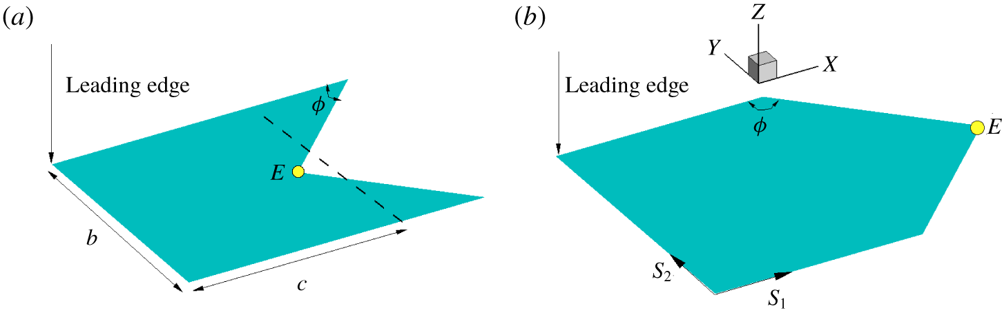
Figure 1 shows the schematic geometry of the flapping flexible plate, which is immersed in a stationary fluid. In our study, the trailing edges are symmetric chevron shapes with concave and convex orientations of varying angle  $\unicode[STIX]{x1D719}$. When
 $\unicode[STIX]{x1D719}=90^{\circ }$, the plate is square with dimensions of
 $b\times c$, where
 $b$ and
 $c$ are the span and mean chord length, respectively. The leading edge of the plate is forced to perform a vertical oscillation described as
 $$\begin{eqnarray}\displaystyle h(t)=A_{0}\cos (2\unicode[STIX]{x03C0}ft), & & \displaystyle\end{eqnarray}$$
where  $A_{0}$ and
 $f$ are the oscillating amplitude and frequency, respectively. Here, a Lagrangian coordinate system
 $(s_{1},s_{2})$ along the plate surface is defined to describe the configuration and motion of the plate.
Schematic diagram of geometries of flapping flexible plates. For all plates in our study, the trailing edges are symmetric chevron shapes with (a) concave ( $\unicode[STIX]{x1D719}<90^{\circ }$) and (b) convex (
 $\unicode[STIX]{x1D719}>90^{\circ }$) orientations. Dimensions
 $b$ and
 $c$ are the span and chord length, respectively. In our study
 $b=c$. For all geometries, the area of the plate is identical, i.e.
 $S=c\times b$. When
 $\unicode[STIX]{x1D719}=90^{\circ }$, the plate is square. Point ‘
 $E$’ denotes the central point of the trailing edge.

Due to the interplay of the plate elasticity, the leading-edge forcing and the forces exerted by the surrounding fluid, the plate begins to move freely and passively in the stationary fluid. The active pitching angle is zero in this model, meaning that only the leading edge of the plate is restricted with a prescribed vertical motion, the remainder of the plate being able to move freely in the entire fluid domain.
To investigate this system of fluid and flapping flexible plate interaction, the incompressible Navier–Stokes equations are solved to simulate the fluid flow:
 $$\begin{eqnarray}\displaystyle & \displaystyle \frac{\unicode[STIX]{x2202}\boldsymbol{v}}{\unicode[STIX]{x2202}t}+\boldsymbol{v}\boldsymbol{\cdot }\unicode[STIX]{x1D735}\boldsymbol{v}=-\frac{1}{\unicode[STIX]{x1D70C}}\unicode[STIX]{x1D735}p+\frac{\unicode[STIX]{x1D707}}{\unicode[STIX]{x1D70C}}\unicode[STIX]{x1D6FB}^{2}\boldsymbol{v}+\boldsymbol{f}, & \displaystyle\end{eqnarray}$$
 $$\begin{eqnarray}\displaystyle & \unicode[STIX]{x1D735}\boldsymbol{\cdot }\boldsymbol{v}=0, & \displaystyle\end{eqnarray}$$
where  $\boldsymbol{v}$ is the velocity,
 $p$ the pressure,
 $\unicode[STIX]{x1D70C}$ the density of the fluid,
 $\unicode[STIX]{x1D707}$ the dynamic viscosity and
 $\boldsymbol{f}$ the body force term.
The structural equation is employed to describe the plate deformation and motion (Huang & Sung Reference Huang and Sung2010; Hua, Zhu & Lu Reference Hua, Zhu and Lu2014; Tang et al. Reference Tang, Huang, Gao and Lu2016):
 $$\begin{eqnarray}\unicode[STIX]{x1D70C}_{s}d\frac{\unicode[STIX]{x2202}^{2}\boldsymbol{X}}{\unicode[STIX]{x2202}t^{2}}=\mathop{\sum }_{i,j=1}^{2}\frac{\unicode[STIX]{x2202}}{\unicode[STIX]{x2202}s_{i}}\left\{\unicode[STIX]{x1D711}_{ij}\left[\unicode[STIX]{x1D6FF}_{ij}-\left(\frac{\unicode[STIX]{x2202}\boldsymbol{X}}{\unicode[STIX]{x2202}s_{i}}\boldsymbol{\cdot }\frac{\unicode[STIX]{x2202}\boldsymbol{X}}{\unicode[STIX]{x2202}s_{j}}\right)^{-1/2}\right]\frac{\unicode[STIX]{x2202}\boldsymbol{X}}{\unicode[STIX]{x2202}s_{j}}-\frac{\unicode[STIX]{x2202}}{\unicode[STIX]{x2202}s_{j}}\left(\unicode[STIX]{x1D6FE}_{ij}\frac{\unicode[STIX]{x2202}^{2}\boldsymbol{X}}{\unicode[STIX]{x2202}s_{i}\unicode[STIX]{x2202}s_{j}}\right)\right\}+\boldsymbol{F}_{s},\end{eqnarray}$$
where  $\boldsymbol{X}(s_{1},s_{2},t)=(X(s_{1},s_{2},t),Y(s_{1},s_{2},t),Z(s_{1},s_{2},t))$ is the position vector of the plate,
 $\boldsymbol{F}_{s}$ is the Lagrangian force exerted on the plate by the surrounding fluid and
 $\unicode[STIX]{x1D70C}_{s}$ and
 $d$ are the mass density and the thickness of the plate. Matrix
 $\unicode[STIX]{x1D711}_{ij}$ is the in-plane effect matrix, where
 $\unicode[STIX]{x1D711}_{11}=\unicode[STIX]{x1D711}_{22}=Ed$ is the stretching stiffness and
 $\unicode[STIX]{x1D711}_{12}=Gd$ is the shearing stiffness of the plate. Matrix
 $\unicode[STIX]{x1D6FE}_{ij}$ is the out-of-plane effect matrix, where
 $\unicode[STIX]{x1D6FE}_{11}=\unicode[STIX]{x1D6FE}_{22}=\unicode[STIX]{x1D6FE}_{12}=EI$ is the bending stiffness of the plate. In addition,
 $\unicode[STIX]{x1D6FF}_{ij}$ is the Kronecker delta function. For the plate, the boundary conditions
 $$\begin{eqnarray}\displaystyle & \displaystyle \unicode[STIX]{x1D711}_{ij}\left[\unicode[STIX]{x1D6FF}_{ij}-\left(\frac{\unicode[STIX]{x2202}\boldsymbol{X}}{\unicode[STIX]{x2202}s_{i}}\boldsymbol{\cdot }\frac{\unicode[STIX]{x2202}\boldsymbol{X}}{\unicode[STIX]{x2202}s_{j}}\right)^{-1/2}\right]\frac{\unicode[STIX]{x2202}X}{\unicode[STIX]{x2202}s_{j}}-\frac{\unicode[STIX]{x2202}}{\unicode[STIX]{x2202}s_{j}}\left(\unicode[STIX]{x1D6FE}_{ij}\frac{\unicode[STIX]{x2202}^{2}X}{\unicode[STIX]{x2202}s_{i}\unicode[STIX]{x2202}s_{j}}\right)=0, & \displaystyle\end{eqnarray}$$
 $$\begin{eqnarray}\displaystyle & \displaystyle Y(t)=Y(0),\quad Z(t)=h(t),\quad \frac{\unicode[STIX]{x2202}\boldsymbol{X}}{\unicode[STIX]{x2202}s_{1}}=(1,0,0) & \displaystyle\end{eqnarray}$$
at the leading edge and
 $$\begin{eqnarray}\displaystyle & \displaystyle \unicode[STIX]{x1D711}_{ij}\left[\unicode[STIX]{x1D6FF}_{ij}-\left(\frac{\unicode[STIX]{x2202}\boldsymbol{X}}{\unicode[STIX]{x2202}s_{i}}\boldsymbol{\cdot }\frac{\unicode[STIX]{x2202}\boldsymbol{X}}{\unicode[STIX]{x2202}s_{j}}\right)^{-1/2}\right]\frac{\unicode[STIX]{x2202}\boldsymbol{X}}{\unicode[STIX]{x2202}s_{j}}-\frac{\unicode[STIX]{x2202}}{\unicode[STIX]{x2202}s_{j}}\left(\unicode[STIX]{x1D6FE}_{ij}\frac{\unicode[STIX]{x2202}^{2}\boldsymbol{X}}{\unicode[STIX]{x2202}s_{i}\unicode[STIX]{x2202}s_{j}}\right)=0, & \displaystyle\end{eqnarray}$$
 $$\begin{eqnarray}\displaystyle & \displaystyle \frac{\unicode[STIX]{x2202}^{2}\boldsymbol{X}}{\unicode[STIX]{x2202}s_{i}\unicode[STIX]{x2202}s_{j}}=0 & \displaystyle\end{eqnarray}$$
at the trailing edge and two other free edges  $s_{2}=0$ or
 $b$ are imposed. Here, the Einstein summation convention is not applied on
 $i$ and
 $j$ (
 $i,j=1,2$). The characteristic quantities
 $\unicode[STIX]{x1D70C}$,
 $c$ and
 $f$ are chosen to normalize the above equations, where
 $\unicode[STIX]{x1D70C}$ is the fluid density,
 $c$ the mean chord length of the plate and
 $f$ the heaving frequency. The characteristic length, speed, time and force are
 $L_{ref}=c$,
 $U_{ref}=cf$,
 $T_{ref}=L_{ref}/U_{ref}=1/f$ and
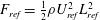 $F_{ref}=\frac{1}{2}\unicode[STIX]{x1D70C}U_{ref}^{2}L_{ref}^{2}$, respectively. It is noted that the characteristic time is equal to the flapping period. The normalized governing parameters are as follows: heaving amplitude
 $A=A_{0}/c$, Reynolds number
 $Re=\unicode[STIX]{x1D70C}fc^{2}/\unicode[STIX]{x1D707}$, stretching coefficient
 $S=Ed/\unicode[STIX]{x1D70C}f^{2}c^{3}$, bending coefficient
 $K=EI/\unicode[STIX]{x1D70C}f^{2}c^{5}$, mass ratio of plate and fluid
 $M=\unicode[STIX]{x1D70C}_{s}d/\unicode[STIX]{x1D70C}c$ (
 $\unicode[STIX]{x1D70C}_{s}$ is the structure density) and aspect ratio of the plate
 $H=b/c$.
3 Numerical method and validation
The fluid flow is solved by the lattice Boltzmann method (Chen & Doolen Reference Chen and Doolen1998; Hua et al. Reference Hua, Zhu and Lu2014) and the motion of the flexible plate is solved by the finite element method. The immersed boundary scheme is used to couple the two solvers (Peskin Reference Peskin2002; Mittal & Iaccarino Reference Mittal and Iaccarino2005). In the immersed boundary scheme, the body force term  $\boldsymbol{f}$ in (2.2) is used as an interaction force between the fluid and the immersed boundary to enforce the no-slip velocity boundary condition. The Lagrangian force
 $\boldsymbol{F}_{s}$ can be calculated by the feedback loop (Goldstein, Handler & Sirovich Reference Goldstein, Handler and Sirovich1993; Huang & Sung Reference Huang and Sung2010; Huang, Chang & Sung Reference Huang, Chang and Sung2011; Hua et al. Reference Hua, Zhu and Lu2014):
 $$\begin{eqnarray}\boldsymbol{F}_{s}(s_{1},s_{2},t)=\unicode[STIX]{x1D716}\int _{0}^{t}[\boldsymbol{V}_{f}(s_{1},s_{2},t^{\prime })-\boldsymbol{V}_{s}(s_{1},s_{2},t^{\prime })]\,\text{d}t^{\prime }+\unicode[STIX]{x1D701}[\boldsymbol{V}_{f}(s_{1},s_{2},t)-\boldsymbol{V}_{s}(s_{1},s_{2},t)],\end{eqnarray}$$
where  $\unicode[STIX]{x1D716}$ and
 $\unicode[STIX]{x1D701}$ are parameters that are selected based on previous studies (Gao & Lu Reference Gao and Lu2008; Tian et al. Reference Tian, Luo, Zhu, Liao and Lu2011; Hua et al. Reference Hua, Zhu and Lu2013),
 $\boldsymbol{V}_{s}=\unicode[STIX]{x2202}\boldsymbol{X}/\unicode[STIX]{x2202}t$ is the plate velocity and
 $\boldsymbol{V}_{f}$ is the fluid velocity at the position of the plate obtained by interpolation:
 $$\begin{eqnarray}\displaystyle \boldsymbol{V}_{f}(s_{1},s_{2},t)=\int \boldsymbol{v}(\boldsymbol{x},t)\unicode[STIX]{x1D6FF}(\boldsymbol{x}-\boldsymbol{X}(s_{1},s_{2},t)]\,\text{d}\boldsymbol{x}. & & \displaystyle\end{eqnarray}$$
Use of the Dirac delta function transforms the Lagrangian force  $\boldsymbol{F}_{s}$ to the Eulerian form
 $$\begin{eqnarray}\displaystyle \boldsymbol{f}(\boldsymbol{x},t)=-\int \boldsymbol{F}_{s}(\boldsymbol{x},t)\unicode[STIX]{x1D6FF}(\boldsymbol{x}-\boldsymbol{X}(s_{1},s_{2},t)]\,\text{d}s_{1}\,\text{d}s_{2}. & & \displaystyle\end{eqnarray}$$
Then the interaction forces  $\boldsymbol{f}(\boldsymbol{x},t)$ and
 $\boldsymbol{F}_{s}(s_{1},s_{2},t)$ obtained from (3.3) and (3.1) are applied to (2.2) and (2.4), respectively.
Equation (2.4) for the deformable plate is discretized by a finite element method and the deformation with large displacement of the plate is handled using the co-rotational scheme (Doyle Reference Doyle2001). A detailed description of the numerical method can be found in our previous studies (Hua et al. Reference Hua, Zhu and Lu2013, Reference Hua, Zhu and Lu2014).
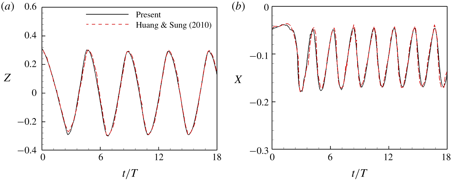
The numerical strategy used here has been successfully applied to a wide range of flows, such as locomotion of a flapping flexible plate (Hua et al. Reference Hua, Zhu and Lu2013), dynamics of fluid flow over a circular flexible plate (Hua et al. Reference Hua, Zhu and Lu2014), dynamics of an inverted flexible plate (Tang, Liu & Lu Reference Tang, Liu and Lu2015) and a multi-inverted flexible plate (Huang, Wei & Lu Reference Huang, Wei and Lu2018), dynamics of a self-propelled plate under the ground effect for the three-dimensional case (Tang et al. Reference Tang, Huang, Gao and Lu2016) and two-dimensional case (Zhang, Huang & Lu Reference Zhang, Huang and Lu2017) and the collective behaviour of multiple flexible plates (Peng, Huang & Lu Reference Peng, Huang and Lu2018). To further validate the numerical method, a flapping flag in a uniform flow (Huang & Sung Reference Huang and Sung2010) was simulated with  $Re=100$,
 $M=1.0$,
 $H=1.0$,
 $S=1000$ and
 $K=0.0001$. Figure 2 shows the time history of the transverse displacements of the lower corner and the streamwise displacements of the centre of the trailing edge of the plate. It is seen that the displacements are consistent with those in Huang & Sung (Reference Huang and Sung2010).
Comparison of the present results and previous data for the time history of (a) the transverse displacements of the lower corner and (b) the streamwise displacements of the centre of the trailing edge of the plate for  $H=1.0$,
 $M=1.0$,
 $S=1000$,
 $K=0.0001$ and
 $Re=100$.

A finite moving computational domain is used in the  $x$ direction to allow the plate to move for a sufficiently long time. As the plate travels one lattice in the
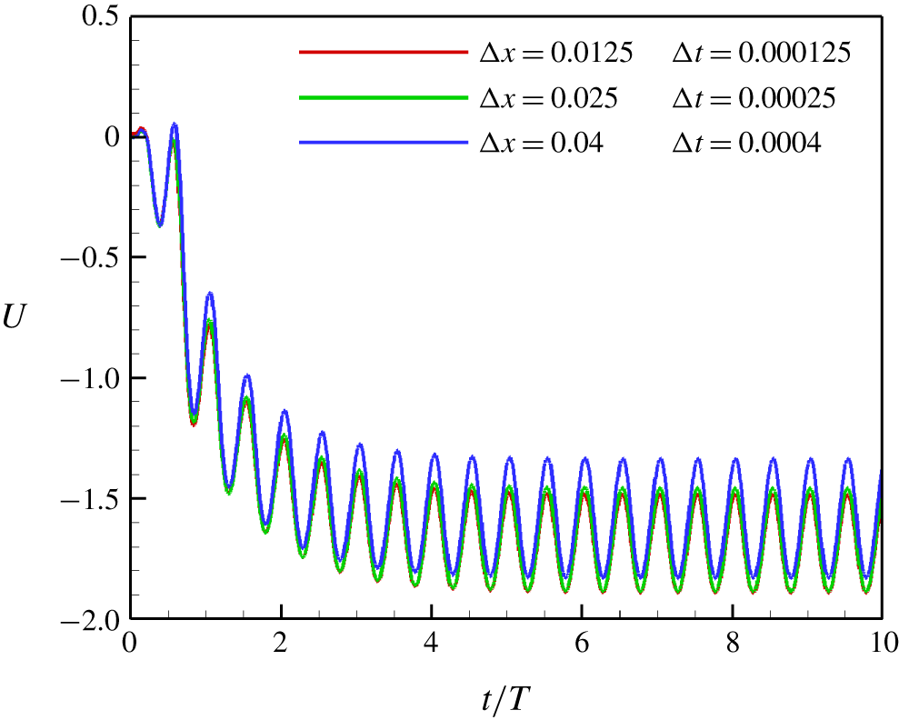
 $x$ direction, the computational domain is shifted, i.e. one layer being added at the inlet and another layer being removed at the outlet (Zhang et al. Reference Zhang, Liu and Lu2010; Hua et al. Reference Hua, Zhu and Lu2013). For the grid and time step independence study, cases with three different sets of
 $\unicode[STIX]{x0394}x$ and
 $\unicode[STIX]{x0394}t$ were tested, i.e.
 $\unicode[STIX]{x0394}x=0.0125$,
 $\unicode[STIX]{x0394}t=0.000125$;
 $\unicode[STIX]{x0394}x=0.025$,
 $\unicode[STIX]{x0394}t=0.00025$;
 $\unicode[STIX]{x0394}x=0.04$,
 $\unicode[STIX]{x0394}t=0.0004$. The propulsive velocity of the self-propelled plate
 $U$ is presented in figure 3. It is shown that the curve of
 $\unicode[STIX]{x0394}x=0.04$ has obvious discrepancies with that of
 $\unicode[STIX]{x0394}x=0.025$, while the curve of
 $\unicode[STIX]{x0394}x=0.025$ is very close to that of
 $\unicode[STIX]{x0394}x=0.0125$.
Grid independence and time step independence study. Propulsive velocity of a flapping flexible plate as a function of time. In these cases,  $\unicode[STIX]{x1D719}=90^{\circ }$,
 $M=0.5$,
 $A=0.2$,
 $S=1000$ and
 $K=5$.

Hence, the results of the convergence tests show that  $\unicode[STIX]{x0394}x=0.025$ and
 $\unicode[STIX]{x0394}t=0.00025$ are small enough to obtain accurate results. In all of the following numerical simulations,
 $\unicode[STIX]{x0394}x=0.025$ and
 $\unicode[STIX]{x0394}t=0.00025$ are adopted. In the simulations, the Neumann boundary condition
 $\unicode[STIX]{x2202}\boldsymbol{v}/\unicode[STIX]{x2202}x=0$ is applied at the outlet and the Dirichlet boundary condition
 $\boldsymbol{v}=0$ is applied at the inlet and four other boundaries. To minimize the effect of boundary conditions, the non-dimensional computational domain for the fluid flow is chosen as
 $[-10,30]\times [-10,10]\times [-10,10]$ in the
 $x$,
 $y$ and
 $z$ directions.
4 Results and discussion
In our study, the Reynolds number is fixed to be  $Re=100$ and the plate is inextensible with a large stretching coefficient
 $S=1000$. The heaving amplitude, mass ratio and aspect ratio are fixed to be
 $A=0.2$,
 $M=0.5$ and
 $H=1$. In nature, the density ratio of a fish tail and fluid (
 $M$) should be small, e.g. 0.05. However, due to the present weak coupling scheme for fluid–structure interaction, numerical instability may be encountered at small
 $M$, e.g.
 $M=0.1$. On the other hand, according to the study of Zhang, Zhou & Luo (Reference Zhang, Zhou and Luo2017) for an elastic panel oscillating in a stream, the propulsive performance of the case with
 $M=0.5$ is close to that with
 $M=0.05$. Hence, some inherent fluid mechanism in self-propulsion of a flexible plate may be revealed through cases of
 $M=0.5$. Other parameters in this study are
 $K\in (2,50)$ (bending coefficient) and
 $\unicode[STIX]{x1D719}\in (30^{\circ },150^{\circ })$ with an interval of
 $15^{\circ }$ (Van Buren et al. Reference Van Buren, Floryan, Brunner, Senturk and Smits2017).
4.1 Propulsive performance
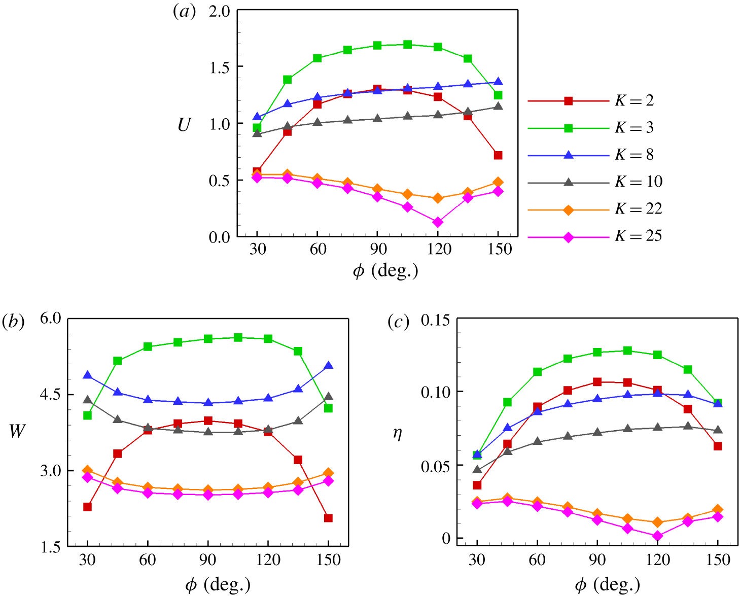
The normalized time-averaged propulsive velocity  $U$ of the plate as a function of
 $\unicode[STIX]{x1D719}$ is shown in figure 4(a). It is seen that for a specific
 $K$, the change mode of
 $U$ as a function of
 $\unicode[STIX]{x1D719}$ may be different. When
 $K$ is relatively small, e.g.
 $K=3$,
 $U$ increases and then decreases with increasing
 $\unicode[STIX]{x1D719}$. There is an optimal
 $\unicode[STIX]{x1D719}$ (
 $\unicode[STIX]{x1D719}_{opt}$) at which the plate achieves the largest
 $U$. We can see that when
 $K=2$,
 $\unicode[STIX]{x1D719}_{opt}\approx 90^{\circ }$ and
 $\unicode[STIX]{x1D719}_{opt}\approx 105^{\circ }$ for
 $K=3$. Hence, it seems that
 $\unicode[STIX]{x1D719}_{opt}$ may be a function of
 $K$. The trailing-edge shape with
 $\unicode[STIX]{x1D719}\approx 90^{\circ }$ having the best performance is also supported by the following fact. Popular freshwater pet fish, such as guppies, mollies, platies and killifish, usually have very flexible tails and their tails look like square plates or slightly convex plates.
When  $K$ is moderate, e.g.
 $K=8$, we can see from figure 4(a) that
 $U$ increases monotonically with increasing
 $\unicode[STIX]{x1D719}$ in the region
 $\unicode[STIX]{x1D719}\in [30^{\circ },150^{\circ }]$. The variation mode is consistent with that in Lauder et al. (Reference Lauder, Lim, Shelton, Witt, Anderson and Tangorra2011). It is also seen that
 $\unicode[STIX]{x1D719}_{opt}$ may be beyond
 $150^{\circ }$ at moderate
 $K$. When
 $K$ is large,
 $U$ decreases with
 $\unicode[STIX]{x1D719}$ until
 $\unicode[STIX]{x1D719}=120^{\circ }$ then rises again. This trend seems more obvious when
 $K$ is larger. This indicates that in the large-
 $K$ region, a concave trailing edge is favourable for enhancing the propulsive speed. This phenomenon coincides with reality: fish with concave tail shape such as tuna whose tail is sufficient rigid (Fierstine & Walters Reference Fierstine and Walters1968; Westneat & Wainwright Reference Westneat and Wainwright2001). This may be the result of natural selection.
(a) Propulsive velocity  $U$, (b) input work
 $W$ and (c) propulsive efficiency
 $\unicode[STIX]{x1D702}$ as functions of trailing-edge angle (
 $\unicode[STIX]{x1D719}$).

The input work  $W$ in a flapping period as a function of
 $\unicode[STIX]{x1D719}$ is shown in figure 4(b). It is noticed that the oscillation of the leading edge of the plate is the energy input of the system. The input work is necessary to maintain the self-propulsion of the plate because the plate has to overcome the drag force acting on it by the surrounding fluid. It can be calculated through the time integral of power
 $P$ produced by the plate during one flapping period, i.e.
 $$\begin{eqnarray}\displaystyle W=\int _{t_{0}}^{t_{0}+T}P\,\text{d}t=\int _{t_{0}}^{t_{0}+T}\iint \boldsymbol{F}_{r}(s_{1},s_{2},t)\boldsymbol{\cdot }\frac{\unicode[STIX]{x2202}\boldsymbol{X}(s_{1},s_{2},t)}{\unicode[STIX]{x2202}t}\,\text{d}s_{1}\,\text{d}s_{2}\,\text{d}t, & & \displaystyle\end{eqnarray}$$
where  $\boldsymbol{F}_{r}$ represents the force on the surrounding fluid from the flapping plate. From figure 4(a,b), it is seen that, generally speaking, the greater the input work, the larger the propulsive speed.
At small  $K$, the trend of the change in input work with
 $\unicode[STIX]{x1D719}$ is identical to that of
 $U$ in figure 4(a). Plates with
 $K=2$ and 3 consume most input work at
 $\unicode[STIX]{x1D719}\approx 90^{\circ }$ and
 $105^{\circ }$, respectively. At these specific trailing-edge angles, the plates achieve their maximal
 $U$. At moderate and large
 $K$, the input work decreases with
 $\unicode[STIX]{x1D719}$ until
 $\unicode[STIX]{x1D719}=90^{\circ }$ then increases. In other words, the input works of the concave and convex plates are larger than that of the square plate at moderate and large
 $K$.
To further quantify the propulsive performance, the propulsive efficiency of a plate  $\unicode[STIX]{x1D702}$ is usually defined as the ratio between the kinetic energy of the body and the input work (Kern & Koumoutsakos Reference Kern and Koumoutsakos2006; Zhang et al. Reference Zhang, Liu and Lu2010; Hua et al. Reference Hua, Zhu and Lu2013), i.e.
 $\unicode[STIX]{x1D702}=\frac{1}{2}MU^{2}/W$. The propulsive efficiency as a function of
 $\unicode[STIX]{x1D719}$ is shown in figure 4(c). The trend of the change in
 $\unicode[STIX]{x1D702}$ with
 $\unicode[STIX]{x1D719}$ at small, moderate and large
 $K$ is approximately identical to that of
 $U$ in figure 4(a). At small
 $K$,
 $\unicode[STIX]{x1D702}$ increases and then decreases with
 $\unicode[STIX]{x1D719}$. There is an optimal
 $\unicode[STIX]{x1D719}$ at which the plate achieves the highest efficiency. At moderate
 $K$,
 $\unicode[STIX]{x1D702}$ approximately increases monotonically with increasing
 $\unicode[STIX]{x1D719}$. It seems that more input work of the convex plate is converted into kinetic energy than those of the square and concave plates. At large
 $K$, the propulsive efficiency decreases monotonically with
 $\unicode[STIX]{x1D719}$ until
 $\unicode[STIX]{x1D719}=120^{\circ }$ then increases slightly. Hence, the propulsive performance of the concave plate seems the best at larger
 $K$.
Therefore, three variation modes of  $U$ and
 $\unicode[STIX]{x1D702}$ as a function of
 $\unicode[STIX]{x1D719}$ have been identified. At small, moderate and large
 $K$, the square, convex and concave plates approximately achieve the best performance, respectively.
4.2 Analysis of flow field
The propulsive performance of a flapping plate may be closely associated with vortical structures. Therefore, in this section we further discuss the effects of the trailing-edge shape on the vortical structures around the plate and the time-averaged velocity field. Here, three typical cases with  $K=3$, 8 and 25 are chosen for small, moderate and large bending stiffness cases, respectively.
4.2.1 The wake topology at moderate  $K$

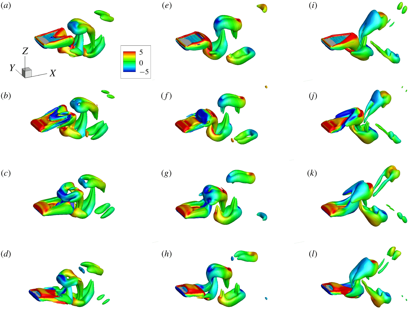
The vortical structures for plates of  $K=8$ at four typical instants during a flapping period are shown in figure 5. In the following figures, the isosurface of the vorticity is shown using the
 $Q$ criterion (Jeong & Hussain Reference Jeong and Hussain1995) with
 $Q=3$ and it is also coloured by the spanwise vorticity. Plates of
 $\unicode[STIX]{x1D719}=30^{\circ }$,
 $90^{\circ }$ and
 $150^{\circ }$ are chosen to represent concave, square and convex plates, respectively. The vortical structures for the plates of
 $\unicode[STIX]{x1D719}=30^{\circ }$ are shown in figure 5(a–d). The wake is composed of two sets of horseshoe-like structures, but the orientation of these horseshoe-like structures is opposite to the wake of a pitching rectangular plate (Buchholz & Smits Reference Buchholz and Smits2006, Reference Buchholz and Smits2008), so they are called ‘reversed horseshoe vortices’.
The vortical structures of the square plate are shown in figure 5(e–h). During half of a period, the vortex is generated at the leading edge and then convected to the trailing edge. Due to the pressure difference between the upper and lower surfaces of the plate, fluid may flow from high-pressure region to low-pressure region from two side edges. Hence, side-edge vortices are generated and shed off together with the trailing-edge vortex , and then a vortex ring forms.
Due to the small aspect ratio, the vortex ring is dominated by side-edge vortices, so the vortex ring is stretched thinner forming an elongated loop. The wake behind the square plate consists of two sets of vortex rings, which are convected downstream at an oblique angle relative to the wake centreline. In addition, each vortex ring has two vortex ‘contrails’. One is at the front of its upstream and the other is at the end of its downstream. They may extend to two neighbouring counter-rotating vortex rings. The contrails become weaker and finally disappear when the vortex ring convects downstream.
The vortical structures for the plate of  $\unicode[STIX]{x1D719}=150^{\circ }$ are shown in figure 5(i–l). It is seen that the vortex generated at the leading edge is convected to the trailing edge. The two side-edge vortices meet at the tip of the trailing edge, then are shed off with the trailing-edge vortex and approximately form a closed ring. When the vortices are further convected downstream, the vortex ring becomes weaker, e.g. only two separated vortical tubes are left. Eventually the vortices would disappear due to viscous dissipation.
Snapshots of instantaneous vortical structures for a plate of (a–d)  $\unicode[STIX]{x1D719}=30^{\circ }$, (e–h)
 $\unicode[STIX]{x1D719}=90^{\circ }$ and (i–l)
 $\unicode[STIX]{x1D719}=150^{\circ }$ with
 $K=8$. Top to bottom rows represent four specific instants during a flapping period: (a,e,i)
 $t/T=0$, (b,f,j)
 $t/T=0.25$, (c,g,k)
 $t/T=0.5$ and (d,h,l)
 $t/T=0.75$. In all snapshots, the isosurface of the
 $Q$ criterion with
 $Q=3$ is shown and it is coloured by the spanwise vorticity.

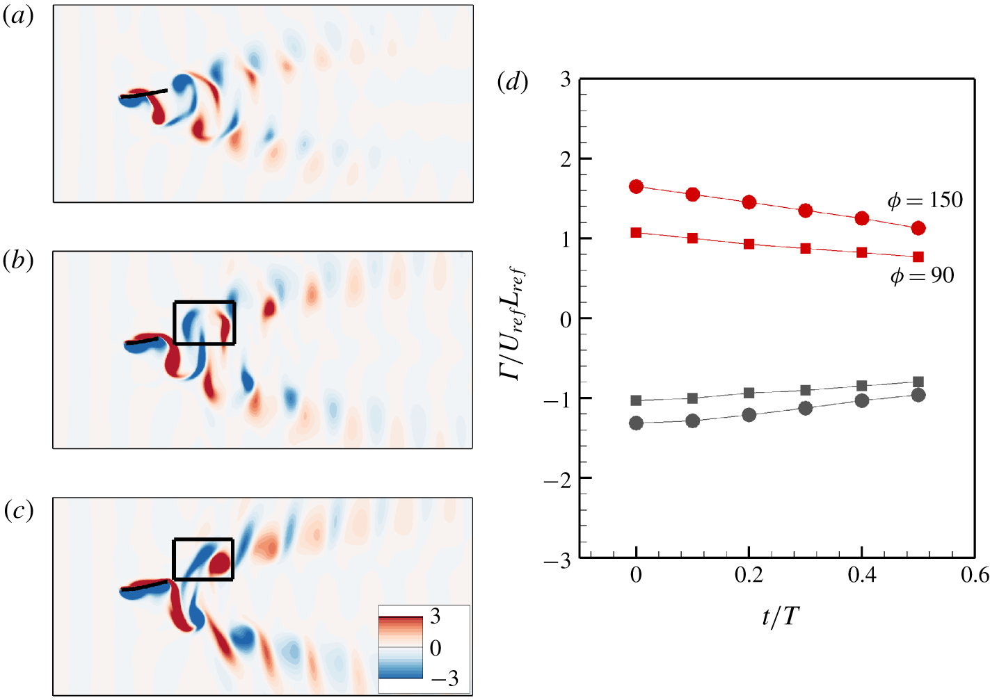
To compare the vortical structures quantitatively, we analyse the instantaneous vorticity contours on the spanwise symmetric plane. The spanwise vorticity contours at  $t/T=0$ on each symmetric plane for the plates of
 $\unicode[STIX]{x1D719}=30^{\circ }$,
 $90^{\circ }$ and
 $150^{\circ }$ are shown in figure 6(a–c) for
 $K=8$. From figure 6(a) we can see that for the concave plate (
 $\unicode[STIX]{x1D719}=30^{\circ }$), the vortex street is the shortest among the three cases (see figure 6b,c) and the vortex dissipates quickly. Therefore the momentum of the jet is small. According to Newton’s third law, the forward momentum of the plate should be small. Hence,
 $U$ is the smallest among the cases.
The circulations of the vortex pairs in the black frames in figure 6(b,c) as functions of time during  $t/T\in (0,0.5)$ are shown in figure 6(d). It is seen that for the cases of
 $\unicode[STIX]{x1D719}=90^{\circ }$ and
 $150^{\circ }$, both vortical strengths decrease with time. For the square plate, the absolute circulations of the positive and negative vortices in the vortex pair are almost identical. However, for the convex plate (
 $\unicode[STIX]{x1D719}=150^{\circ }$), the absolute circulation of the positive vortex is significantly larger than that of the negative vortex. This may result in a clockwise rotation of the vortex pair and then the dipole-induced velocity in the
 $x$ direction will increase. This is helpful for the plate’s forward propulsion.
The instantaneous spanwise vorticity contours at  $t/T=0$ for cases with (a)
 $\unicode[STIX]{x1D719}=30^{\circ }$, (b)
 $\unicode[STIX]{x1D719}=90^{\circ }$ and (c)
 $\unicode[STIX]{x1D719}=150^{\circ }$ for
 $K=8$. (d) The circulation of the vortex pairs in black frames in (b,c) as a function of time. Filled squares and circles represent
 $\unicode[STIX]{x1D719}=90^{\circ }$ and
 $150^{\circ }$, respectively. Red and grey represent positive and negative vortices, respectively.

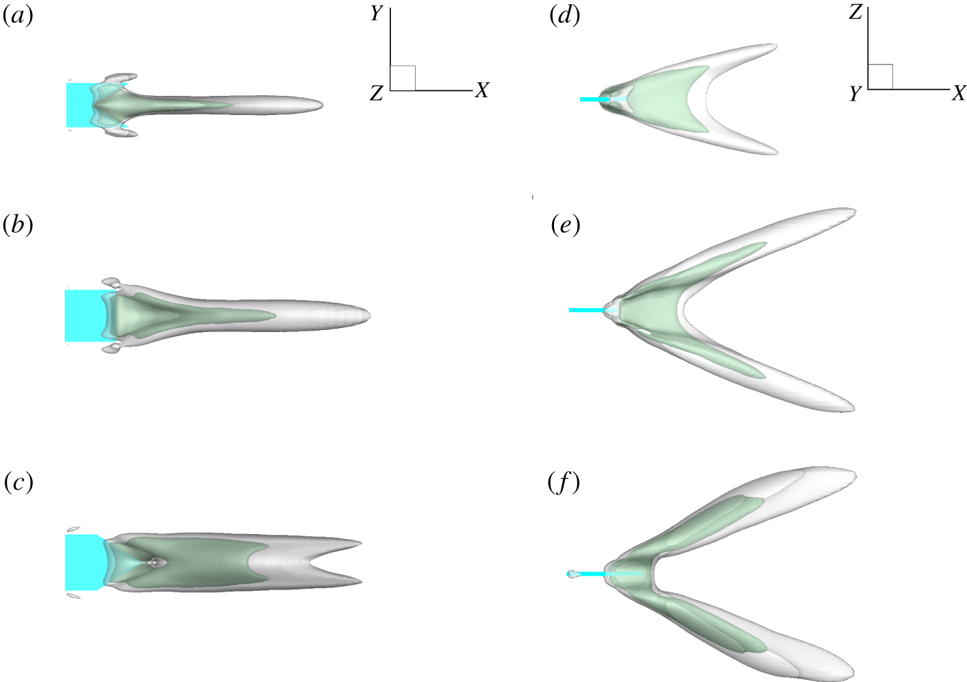
The isosurfaces of time-averaged streamwise velocity  $\bar{u}_{x}$ for the plates of
 $\unicode[STIX]{x1D719}=30^{\circ }$,
 $90^{\circ }$ and
 $150^{\circ }$ are shown in figure 7(a–c) for
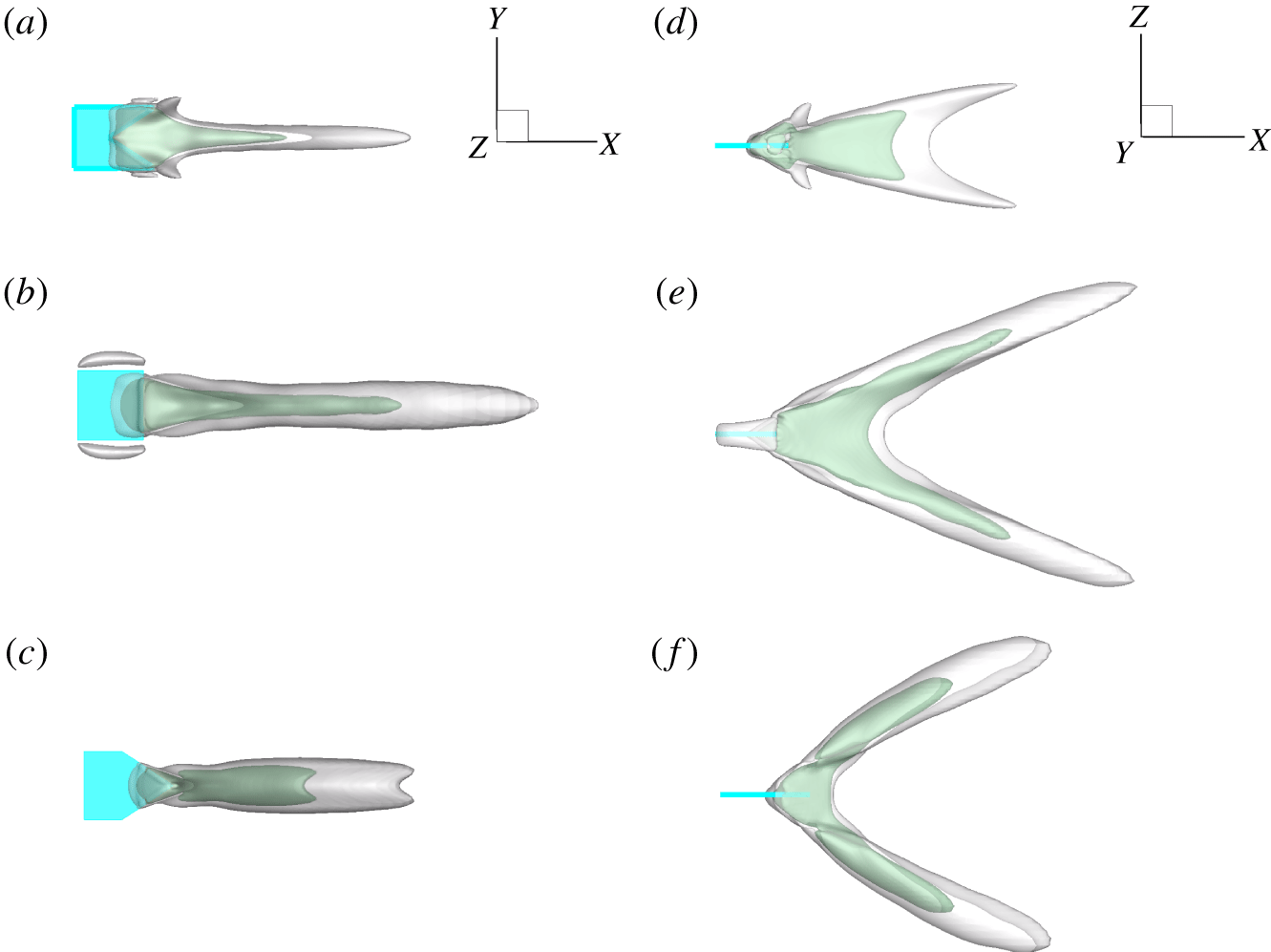
 $K=8$, respectively. From the side views, it can be seen that all the wakes develop to form bifurcated jets with different inclination angles. For the plate of
 $\unicode[STIX]{x1D719}=30^{\circ }$, although the inclination angle is the smallest among the three cases, the length of the jet is the shortest. According to Newton’s third law, the propulsive performance of the concave plate would not be so good. On the other hand, the jet behind the convex plate is wider and longer than that of the square plate. Furthermore, the inclination of the jet behind the convex plate is slightly smaller than that of the square plate, so the convex plate has a better propulsive performance than the square plate.
Isosurfaces of time-averaged streamwise velocity  $\bar{u}_{x}$ thresholded at
 $\bar{u}_{x}=5$ (grey) and 10 (green) for
 $K=8$. (a–c) Top views and (d–f) side views. The upper, middle and lower rows are the cases with
 $\unicode[STIX]{x1D719}=30^{\circ }$,
 $90^{\circ }$ and
 $150^{\circ }$, respectively.

The effect of trailing-edge shape on the propulsive performance of plates at moderate  $K$ is consistent with the result of experiments for a heaving flexible foil in a stream (Lauder et al. Reference Lauder, Lim, Shelton, Witt, Anderson and Tangorra2011). It has also been shown that the performance of the convex plate is the best at moderate
 $K$.
4.2.2 The wake topology at small $K$

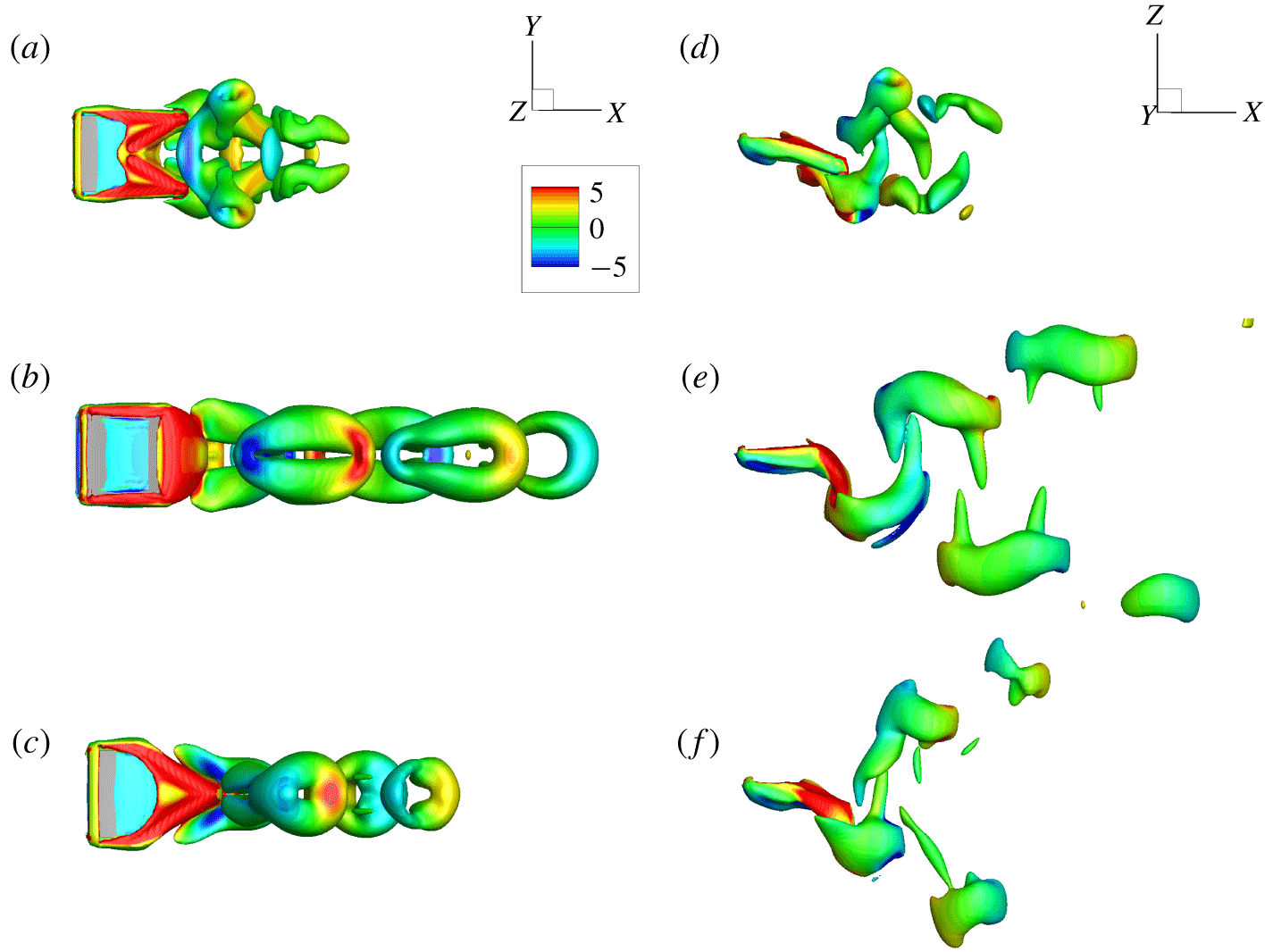
Typical vortical structures for the plates of  $K=3$ at the beginning of the flapping period (
 $t/T=0$) are shown in figure 8. Typical results for the concave, square and convex plates are presented. Figure 8(a,d) shows that for the concave plate (
 $\unicode[STIX]{x1D719}=30^{\circ }$), the vortex street is short, and the wake is composed of two sets of reversed horseshoe vortices, which is similar to the vortex structure in Li, Zhu & Lu (Reference Li, Zhu and Lu2012) for forked fins. On the other hand, it is also seen from figure 8(a) that besides the reversed horseshoe vortices, there are additional small vortical structures at two spanwise tips, which are attached to the reversed horseshoe vortex. The minor difference between the present vortical structure and that in Li et al. (Reference Li, Zhu and Lu2012) may be due to the spanwise deformation of the two ‘lobes’ of trailing edges at small
 $K$ in our study. It is noticed that at moderate
 $K$ there are no such small vortical structures (see figure 5a–d).
For the square plate ( $\unicode[STIX]{x1D719}=90^{\circ }$), figure 8(b,e) shows that the wake consists of two sets of vortex rings. The vortical structure is similar to that of the square plate at moderate
 $K$ (see the middle column of figure 5) except here the vortex street seems longer. For the convex plate (
 $\unicode[STIX]{x1D719}=150^{\circ }$), figure 8(c,f) shows that the wake is also composed of vortex rings. The vortical structure looks like that of the square plate (
 $\unicode[STIX]{x1D719}=90^{\circ }$), but the vortex rings here are closer to circular rings. The side views of the vortical structures in figure 8(d–f) show that all the vortical structures are convected downstream at an oblique angle relative to the wake centreline.
Top views (a–c) and side views (d–f) of vortical structures for (a,d) the concave plate ( $\unicode[STIX]{x1D719}=30^{\circ }$), (b,e) the square plate (
 $\unicode[STIX]{x1D719}=90^{\circ }$) and (c,f) the convex plate (
 $\unicode[STIX]{x1D719}=150^{\circ }$) with
 $K=3$ at
 $t/T=0$. In all snapshots, the isosurface of the
 $Q$ criterion with
 $Q=3$ is shown and it is coloured by the spanwise vorticity.

The isosurfaces of time-averaged streamwise velocity for the plates with  $\unicode[STIX]{x1D719}=30^{\circ }$,
 $90^{\circ }$ and
 $150^{\circ }$ for
 $K=3$ are shown in figure 9(a–c), respectively. The side views show that for each case, there is a bifurcated jet behind the plate with an inclined angle to the wake centreline. For the plate of
 $\unicode[STIX]{x1D719}=30^{\circ }$, although the inclination angle is the smallest among the three cases, the length of the jet is the shortest. Hence, the propulsive speed may still be small. On the other hand, the jet behind the square plate is longer and wider than those of the concave and convex cases. Besides, figure 9(d–f) shows that the inclination angle of the jet behind the square plate is smaller than that of the convex plate. Hence, the square plate achieves the best propulsive performance among the three plates.
Isosurfaces of normalized time-averaged streamwise velocity  $\bar{u}_{x}$ thresholded at
 $\bar{u}_{x}=5$ (grey) and 10 (green) for
 $K=3$. (a–c) Top views and (d–f) side views. The upper, middle and lower rows represent the cases of the concave plate (
 $\unicode[STIX]{x1D719}=30^{\circ }$), the square plate (
 $\unicode[STIX]{x1D719}=90^{\circ }$) and the convex plate (
 $\unicode[STIX]{x1D719}=150^{\circ }$), respectively.

4.2.3 The wake topology at large $K$

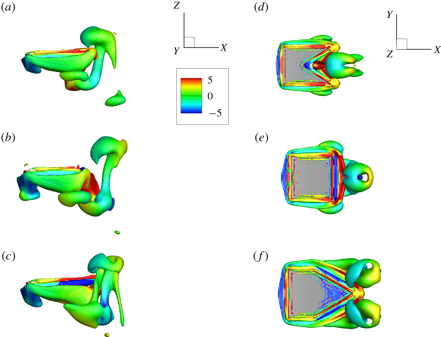
Typical vortical structures for plates with  $K=25$ at the beginning of the flapping period (
 $t/T=0$) are shown in figure 10. It is seen that the vortex street is very short. Accordingly, the propulsive velocity of plates with
 $K=25$ is small.
For concave ( $\unicode[STIX]{x1D719}=30^{\circ }$) and square (
 $\unicode[STIX]{x1D719}=90^{\circ }$) plates, the wakes are composed of two sets of reversed horseshoe vortices and vortex rings, respectively. The wakes are shorter than those at moderate
 $K$. From the side views, it is also noticed that the leading-edge vortices in the cases with
 $K=25$ are clearer than those in the cases with
 $K=8$. From figure 10(c,f), it is seen that the wake behind the trailing edge of the convex plate (
 $\unicode[STIX]{x1D719}=150^{\circ }$) consists of a twisted vortical structure, which may be evolved from the side-edge vortices.
Side views (a–c) and top views (d–f) for snapshots of vortical structures for (a,d) the plate of  $\unicode[STIX]{x1D719}=30^{\circ }$, (b,e) the plate of
 $\unicode[STIX]{x1D719}=90^{\circ }$ and (c,f) the plate of
 $\unicode[STIX]{x1D719}=150^{\circ }$ with
 $K=25$ at
 $t/T=0$. In all snapshots, the isosurface of the
 $Q$ criterion with
 $Q=3$ is shown and it is coloured by spanwise vorticity.

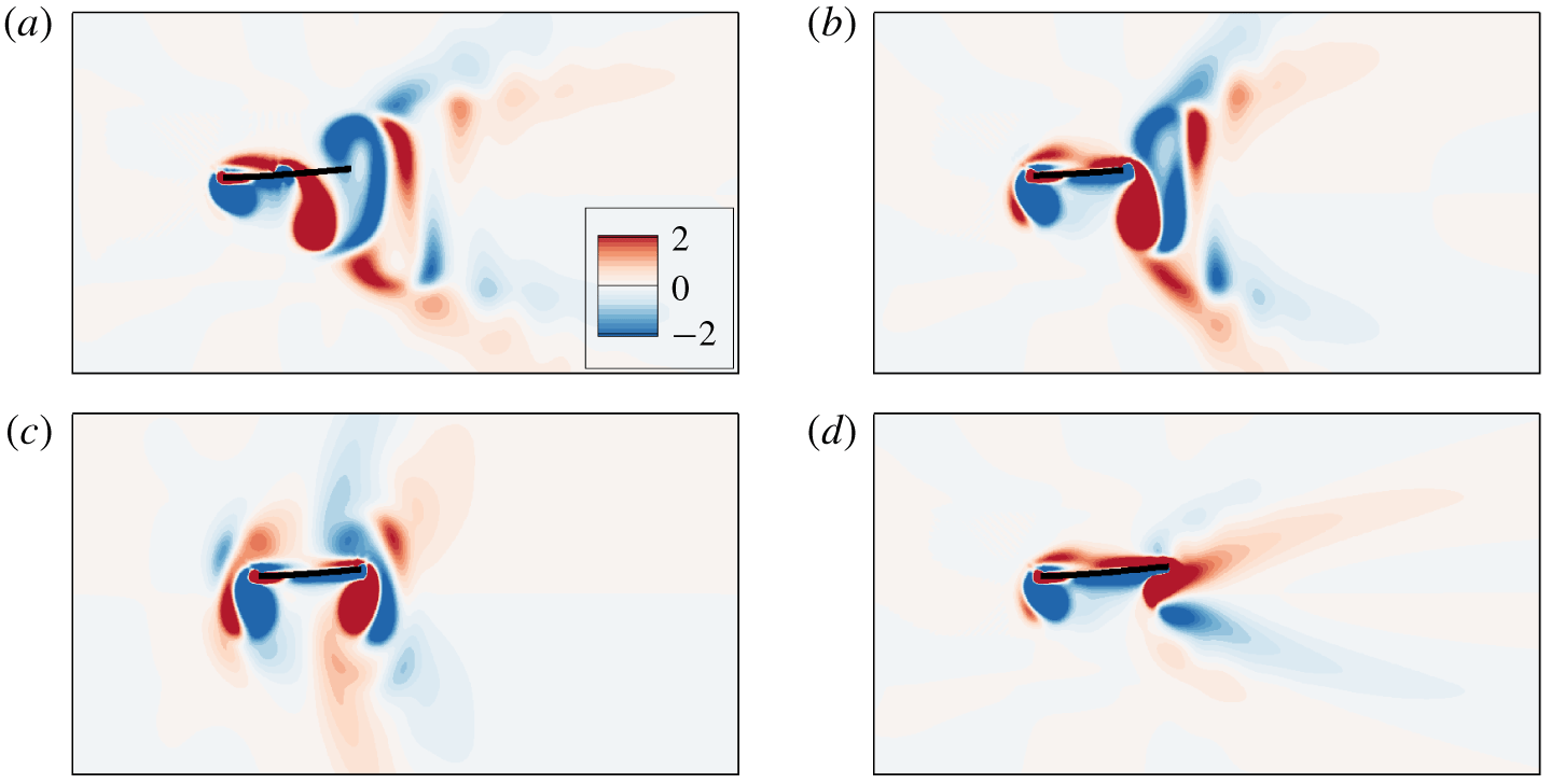
To further investigate the effect of trailing-edge shape on the leading-edge vortices, the spanwise vorticity contours at  $t/T=0$ on the spanwise symmetric plane for cases with
 $\unicode[STIX]{x1D719}=30^{\circ }$,
 $90^{\circ }$,
 $120^{\circ }$ and
 $150^{\circ }$ are shown in figure 11. It seems that the strength of the leading-edge vortices increases with
 $\unicode[STIX]{x1D719}$ when
 $\unicode[STIX]{x1D719}<120^{\circ }$.
From figure 11(c), it is seen that when  $\unicode[STIX]{x1D719}=120^{\circ }$ the vorticity of the leading-edge vortex is almost as large as that of the trailing-edge vortex and the flow field around the plate is almost symmetric. The symmetric flow field is not favourable for generating thrust force (Vandenberghe et al. Reference Vandenberghe, Zhang and Childress2004; Alben & Shelley Reference Alben and Shelley2005). Hence, propulsive speed in the case of
 $\unicode[STIX]{x1D719}=120^{\circ }$ is small. On the other hand, the flow fields in figure 11(a,b,d) are not symmetric and the generated thrust would push the plate to move horizontally. Since the deformation of the plate is small at large
 $K$, the situation is almost identical to the rigid flapping foil in the work of Alben & Shelley (Reference Alben and Shelley2005). The work has shown that the self-propelled foil may move forward as a result of the asymmetric flow field around the foil. In the asymmetric flow field, an inverted von Kármán vortex street occurs in the wake which drives the horizontal movement of the foil.
The spanwise vorticity contours at the beginning of the flapping period for plates with (a)  $\unicode[STIX]{x1D719}=30^{\circ }$, (b)
 $\unicode[STIX]{x1D719}=90^{\circ }$, (c)
 $\unicode[STIX]{x1D719}=120^{\circ }$ and (d)
 $\unicode[STIX]{x1D719}=150^{\circ }$ at
 $K=25$. Red and blue represent positive and negative vortices, respectively.

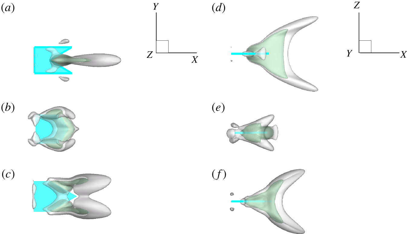
The isosurfaces of time-averaged streamwise velocity for the plates of  $\unicode[STIX]{x1D719}=30^{\circ }$,
 $120^{\circ }$ and
 $150^{\circ }$ are shown in figure 12(a–c), respectively. For the plate of
 $\unicode[STIX]{x1D719}=30^{\circ }$, the jet length is the longest and the inclination angle of the jet is the smallest among the three plates. These factors result in a larger
 $U$. For the plate of
 $\unicode[STIX]{x1D719}=120^{\circ }$, the jet behind the plate is very weak so the propulsive performance of
 $\unicode[STIX]{x1D719}=120^{\circ }$ is worst (see figure 4a,d). For the plate of
 $\unicode[STIX]{x1D719}=150^{\circ }$, the jet is split into four parts corresponding to the vortical structure in figure 10(c,f); it is similar to the time-averaged velocity field in Van Buren et al. (Reference Van Buren, Floryan, Brunner, Senturk and Smits2017). Furthermore, the jet in the case of
 $\unicode[STIX]{x1D719}=150^{\circ }$ is longer and wider than that of
 $\unicode[STIX]{x1D719}=120^{\circ }$, so the propulsive performance in the case of
 $\unicode[STIX]{x1D719}=150^{\circ }$ is better than that in the case of
 $\unicode[STIX]{x1D719}=120^{\circ }$.
Isosurfaces of time-averaged streamwise velocity  $\bar{u}_{x}$ thresholded at
 $\bar{u}_{x}=5$ (grey) and 10 (green) for
 $K=25$. (a–c) Top views and (d–f) side views. The upper, middle and lower rows represent the cases of the concave plate (
 $\unicode[STIX]{x1D719}=30^{\circ }$) and two convex plates (
 $\unicode[STIX]{x1D719}=120^{\circ }$ and
 $\unicode[STIX]{x1D719}=150^{\circ }$), respectively.

4.3 Deformation and surface pressure
For a plate with large  $K$, the deformation of the plate is small and the asymmetry flow field around the plate is supposed to induce horizontal motion (Vandenberghe et al. Reference Vandenberghe, Zhang and Childress2004; Alben & Shelley Reference Alben and Shelley2005). When
 $K$ is small or moderate, deformation of the flexible plate leads to the repartition of the force on the plate compared to the rigid one (Ramananarivo, Godoy-Diana & Thiria Reference Ramananarivo, Godoy-Diana and Thiria2011). In the following, the response of trailing edge and surface pressure for small and moderate
 $K$ will be further discussed to see how the hydrodynamic force contributes to the thrust force.
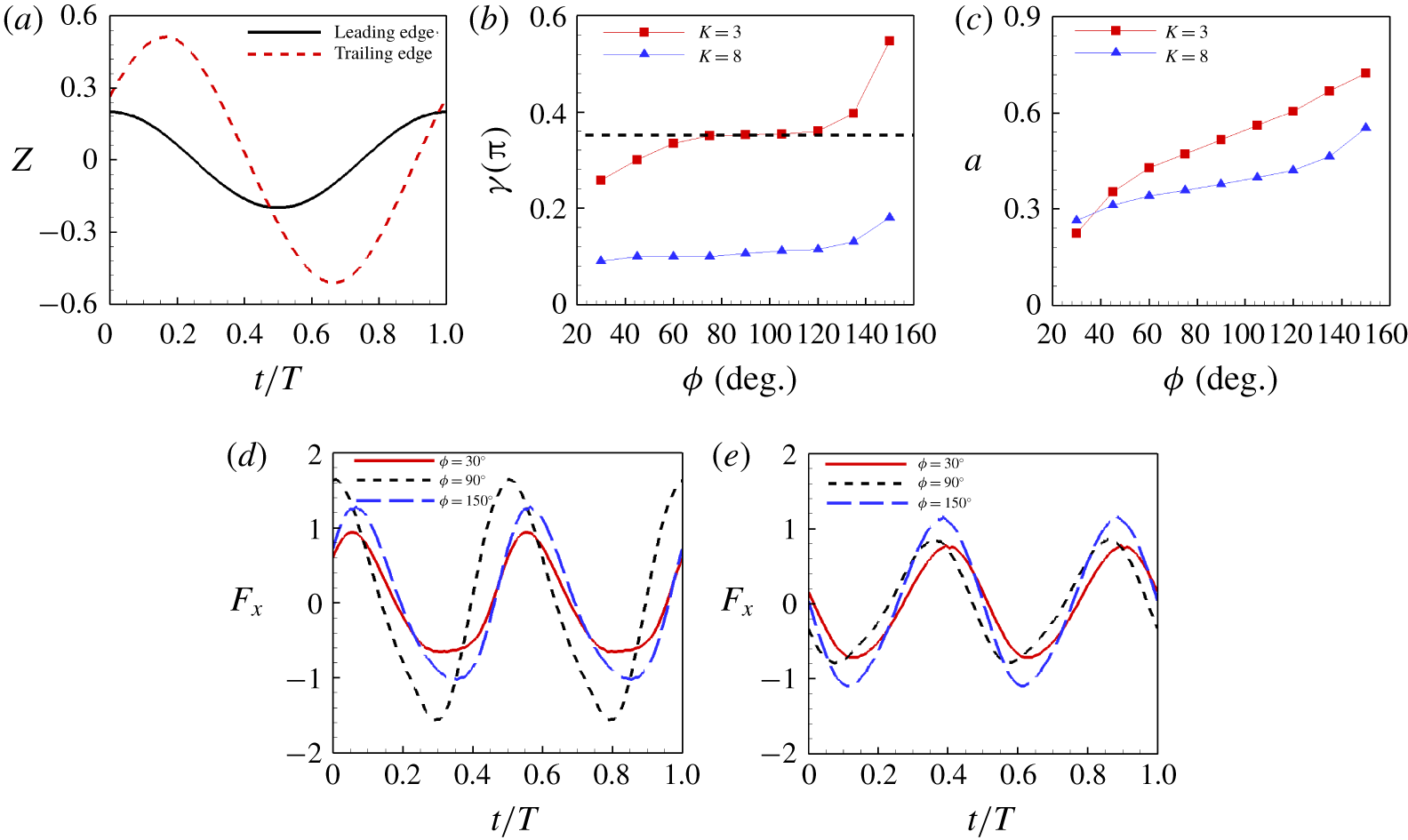
The response of the trailing edge is represented by the transverse motion of the central point of the trailing edge  $E$ (see figure 1). Figure 13(a) shows the time evolution of the transverse motions of the leading and trailing edges for the square plate with
 $K=3$ during a flapping period. It is seen that there is a phase lag between the transverse motions of the leading and trailing edges, which is denoted by
 $\unicode[STIX]{x1D6FE}$. The phase lag may depend on both
 $K$ and
 $\unicode[STIX]{x1D719}$.
The phase lag  $\unicode[STIX]{x1D6FE}$ and flapping amplitude of trailing edge
 $a$ as functions of
 $\unicode[STIX]{x1D719}$ for
 $K=3$ and 8 are shown in figure 13(b,c). It is seen from figure 13(b,c) that both
 $\unicode[STIX]{x1D6FE}$ and
 $a$ for
 $K=3$ and 8 increase monotonically with
 $\unicode[STIX]{x1D719}$. Actually not only
 $a$ but also
 $\unicode[STIX]{x1D6FE}$ affect the propulsive performance. Previous studies have shown that for a flexible plate, the optimal
 $\unicode[STIX]{x1D6FE}\approx 0.25\unicode[STIX]{x03C0}$ (Ramananarivo et al. Reference Ramananarivo, Godoy-Diana and Thiria2011) or
 $0.4\unicode[STIX]{x03C0}$ (Yeh & Alexeev Reference Yeh and Alexeev2014) coupled with a large amplitude
 $a$ would boost the propulsive performance significantly. Our result has shown that the performance of the case with
 $K=3$ and
 $\unicode[STIX]{x1D719}=90^{\circ }$ is the best in all cases that we studied. The corresponding phase lag is
 $\unicode[STIX]{x1D6FE}\approx 0.35\unicode[STIX]{x03C0}$ (see figure 13b), which is consistent with the optimal
 $\unicode[STIX]{x1D6FE}$ in Ramananarivo et al. (Reference Ramananarivo, Godoy-Diana and Thiria2011) and Yeh & Alexeev (Reference Yeh and Alexeev2014). For the plates with moderate
 $K$, e.g.
 $K=8$, all phase lags may be smaller than the optimal one. Under these circumstances, the propulsive performance may be proportional to
 $a$. Hence, the performance increases with
 $\unicode[STIX]{x1D719}$ monotonically.
(a) The transverse motions of the leading and trailing edges at the spanwise symmetry plane as functions of time for the square plate with  $K=3$. (b) Phase lag
 $\unicode[STIX]{x1D6FE}$ and (c) amplitude
 $a$ of the trailing edge as functions of
 $\unicode[STIX]{x1D719}$ for
 $K=3$ and 8. Time evolution of the non-dimensional horizontal force
 $F_{x}$ for
 $\unicode[STIX]{x1D719}=30^{\circ }$,
 $90^{\circ }$ and
 $150^{\circ }$ for (d)
 $K=3$ and (e)
 $K=8$.

Because  $a$ and
 $\unicode[STIX]{x1D6FE}$ seem not so directly relevant to the performance, we analyse the thrust experienced by the plates, which is directly a function of the cruising speed. Figure 13(d,e) shows time evolution of the horizontal forces
 $F_{x}$ experienced by the plates with
 $K=3$ and
 $K=8$. It is noticed that due to the self-propulsion, the integral of
 $F_{x}$ in a flapping period
 $T$ is zero. From figure 13(d,e), it is seen that at
 $K=3$, the plate with
 $\unicode[STIX]{x1D719}=90^{\circ }$, which has the largest
 $U$, experiences the maximal thrust and drag during the period. Whereas at
 $K=8$, the plate with
 $\unicode[STIX]{x1D719}=150^{\circ }$ experiences the maximal thrust and drag.
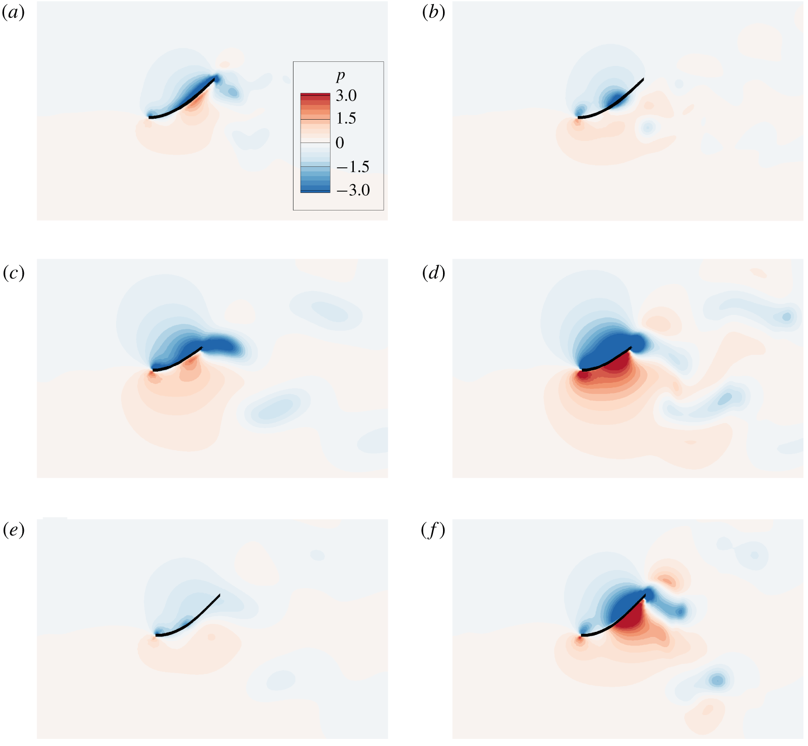
The side views of pressure distributions for  $K=3$ on (a,c,e) the side-edge planes (
 $(x,z)$ planes passing through the side edges) and (b,d,f) the spanwise symmetry planes for (a,b)
 $\unicode[STIX]{x1D719}=30^{\circ }$, (c,d)
 $\unicode[STIX]{x1D719}=90^{\circ }$ and (e,f)
 $\unicode[STIX]{x1D719}=150^{\circ }$ at the moment when each case achieves its own largest thrust.

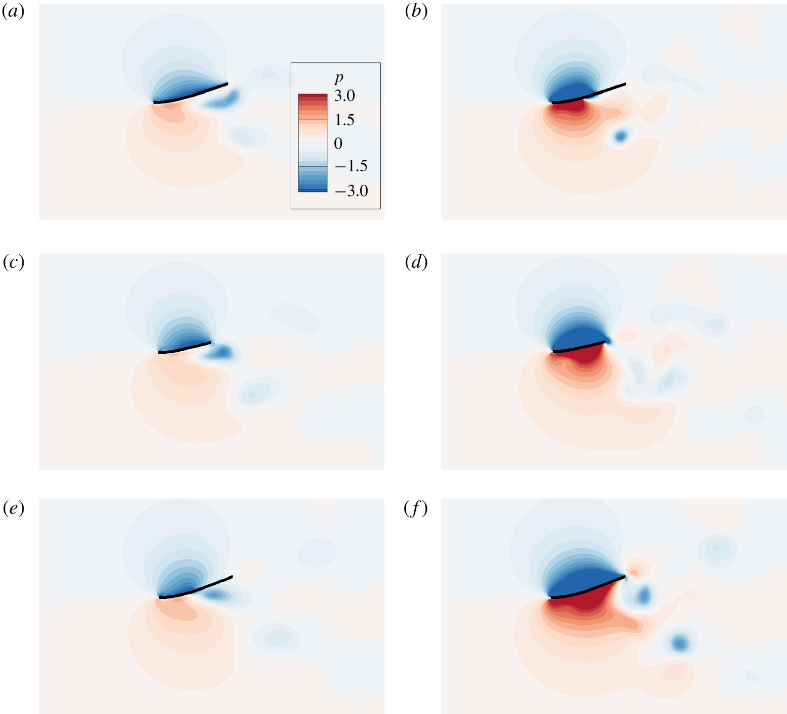
The side views of pressure distributions for  $K=8$ on (a,c,e) the side-edge planes and (b,d,f) the spanwise symmetry planes for (a,b)
 $\unicode[STIX]{x1D719}=30^{\circ }$, (c,d)
 $\unicode[STIX]{x1D719}=90^{\circ }$ and (e,f)
 $\unicode[STIX]{x1D719}=150^{\circ }$ at the moment when each case achieves its own largest thrust.

We analyse the pressure fields to understand why the thrusts in the cases are different. For the cases with  $K=3$, from figure 13(d), we can see the moment when the maximal thrust appears for each case, i.e.
 $t/T=0.35$ for the cases with
 $\unicode[STIX]{x1D719}=30^{\circ }$ and
 $150^{\circ }$ and
 $t/T=0.3$ for the case with
 $\unicode[STIX]{x1D719}=90^{\circ }$. The snapshots of the pressure fields at that moment are shown in figure 14. The snapshots of the side-edge planes (
 $(x,z)$ planes passing through the side edges) and spanwise symmetry planes are shown in figures 14(a,c,e) and 14(b,d,f), respectively. The pressure distributions on the side-edge planes (figure 14a,c,e) show that pressure difference in the case
 $\unicode[STIX]{x1D719}=90^{\circ }$ (figure 14c) is significantly larger than those in the other cases. The pressure distributions on the spanwise symmetry planes (figure 14b,d,f) show that both the low-pressure region above the plate and the high-pressure region below the plate in the case of
 $\unicode[STIX]{x1D719}=90^{\circ }$ are larger than those in the other two cases. Hence, pressure difference in the case of
 $\unicode[STIX]{x1D719}=90^{\circ }$ is the largest among the three cases, which contributes much to the largest thrust.
For the cases with  $K=8$, the pressure fields are also analysed. The snapshots of the pressure fields at the moment when the maximal thrust appears (see figure 13e), i.e.
 $t/T=0.1$ for the cases with
 $\unicode[STIX]{x1D719}=30^{\circ }$ and
 $150^{\circ }$ and
 $t/T=0.05$ for the case with
 $\unicode[STIX]{x1D719}=90^{\circ }$, are shown in figure 15. Figures 15(a,c,e) and 15(b,d,f) are the snapshots of the side-edge planes and spanwise symmetry planes, respectively. The pressure distributions on the side-edge planes in the three cases look similar. Due to the three-dimensional effect, in each case the pressure difference on the spanwise symmetry plane is much larger than that on the side-edge plane. It is also seen that both the low-pressure region above the plate and the high-pressure region below the plate increase with
 $\unicode[STIX]{x1D719}$ (figure 15b,d,f). Besides, the middle chord length increases with
 $\unicode[STIX]{x1D719}$. Hence, the pressure difference would increase with
 $\unicode[STIX]{x1D719}$. In this way, the resultant thrust as well as propulsive performance would also increase with
 $\unicode[STIX]{x1D719}$ at moderate
 $K$.
4.4 Force analysis and the scaling law
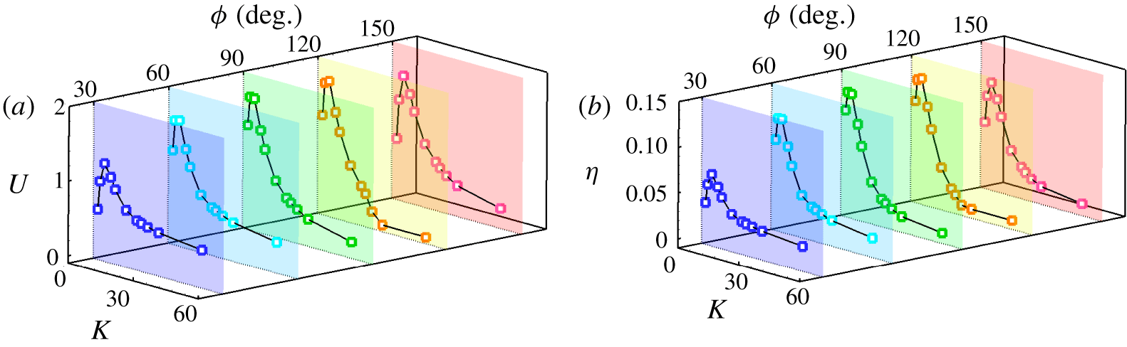
The propulsive velocity  $U$ and efficiency
 $\unicode[STIX]{x1D702}$ as functions of
 $K$ at typical
 $\unicode[STIX]{x1D719}$ are shown in figure 16(a,b). For each typical
 $\unicode[STIX]{x1D719}$, there is an optimal
 $K\in [3,5]$, at which
 $U$ and
 $\unicode[STIX]{x1D702}$ peaks can be achieved. Here the dynamic model proposed in Ramananarivo et al. (Reference Ramananarivo, Godoy-Diana and Thiria2011) is adopted to explain why there is an optimal range of
 $K$.
(a) Propulsive velocity  $U$ and (b) propulsive efficiency
 $\unicode[STIX]{x1D702}$ as functions of
 $K$ and
 $\unicode[STIX]{x1D719}$.

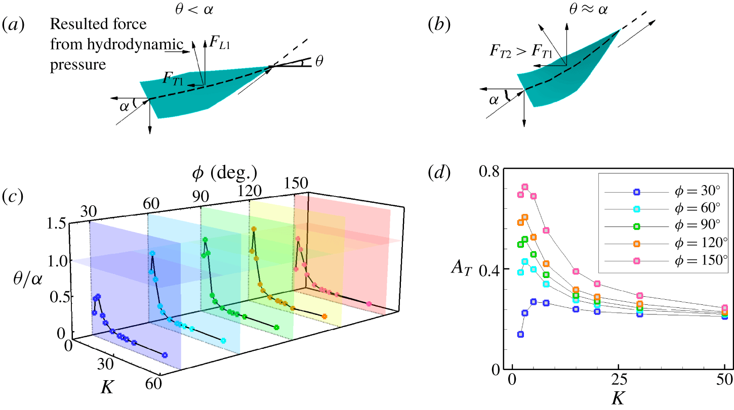
In the dynamic model (figure 17a,b), two characteristic angles  $\unicode[STIX]{x1D6FC}$ and
 $\unicode[STIX]{x1D703}$ about the motion and deformation of the plate are introduced to describe the kinematics of the plate. Angle
 $\unicode[STIX]{x1D6FC}=\arctan (2\unicode[STIX]{x03C0}fA/U^{\prime })$ is the instantaneous angle of attack at the moment when the leading edge is heaving with maximal vertical velocity, where
 $U^{\prime }$ and
 $2\unicode[STIX]{x03C0}fA$ are the instantaneous cruising speed and heaving velocity, respectively, at that moment. Angle
 $\unicode[STIX]{x1D703}$ is the deflection angle at the trailing edge on the spanwise symmetric plane at the same moment. Figures 17(a) and 17(b) show the cases of
 $\unicode[STIX]{x1D703}<\unicode[STIX]{x1D6FC}$ and
 $\unicode[STIX]{x1D703}\approx \unicode[STIX]{x1D6FC}$, respectively. Compared to figure 17(a), figure 17(b) shows that more hydrodynamic force can be projected in the propulsive direction when
 $\unicode[STIX]{x1D703}\approx \unicode[STIX]{x1D6FC}$. Hence
 $\unicode[STIX]{x1D703}/\unicode[STIX]{x1D6FC}\approx 1$ is favourable for achieving higher performance.
Schematic diagrams for the dynamic model (Ramananarivo et al. Reference Ramananarivo, Godoy-Diana and Thiria2011): (a) the case of  $\unicode[STIX]{x1D703}<\unicode[STIX]{x1D6FC}$ and (b) the case of
 $\unicode[STIX]{x1D703}\approx \unicode[STIX]{x1D6FC}$. (c) Ratio
 $\unicode[STIX]{x1D703}/\unicode[STIX]{x1D6FC}$ and (d) the flapping amplitude of the trailing edge as functions of
 $K$ and
 $\unicode[STIX]{x1D719}$.

The value of  $\unicode[STIX]{x1D703}/\unicode[STIX]{x1D6FC}$ as a function of
 $K$ is shown in figure 17(c). It is seen that the trend of
 $\unicode[STIX]{x1D703}/\unicode[STIX]{x1D6FC}$ varying with
 $K$ is similar to those of
 $U$ and
 $\unicode[STIX]{x1D702}$ at each
 $\unicode[STIX]{x1D719}$ (see figure 16a,b). The value of
 $\unicode[STIX]{x1D703}/\unicode[STIX]{x1D6FC}$ is close to unity when
 $K\approx 3$. Hence, the propulsive velocity and efficiency reach their peaks at
 $K\approx 3$. It is noticed that
 $K$ is associated with the frequency ratio
 $\overline{\unicode[STIX]{x1D714}}_{f}=f/f_{1}^{fluid}$, where
 $f_{1}^{fluid}$ and
 $f$ are the first natural frequency in the fluid and the flapping frequency of the plate, respectively. According to the theory proposed in Van Eysden & Sader (Reference Van Eysden and Sader2006), the natural frequency of the plate in the fluid (
 $f_{1}^{fluid}$) can be derived from that in vacuum (
 $f_{1}^{vac}$) as follows:
 $$\begin{eqnarray}\displaystyle & f_{1}^{vac}=C_{1}^{2}/(2\unicode[STIX]{x03C0}c^{2})\sqrt{EI/\unicode[STIX]{x1D70C}_{s}d}, & \displaystyle\end{eqnarray}$$
 $$\begin{eqnarray}\displaystyle & \displaystyle f_{1}^{fluid}=f_{1}^{vac}\left[1+\frac{\unicode[STIX]{x03C0}\unicode[STIX]{x1D70C}b}{4\unicode[STIX]{x1D70C}_{s}d}\unicode[STIX]{x1D6FA}(\unicode[STIX]{x1D709})\right]^{-1/2}, & \displaystyle\end{eqnarray}$$
 $$\begin{eqnarray}\displaystyle & \displaystyle \unicode[STIX]{x1D709}=C_{1}\frac{b}{c}, & \displaystyle\end{eqnarray}$$
 $$\begin{eqnarray}\displaystyle & \displaystyle \unicode[STIX]{x1D6FA}(\unicode[STIX]{x1D709})=\frac{1+0.74273\unicode[STIX]{x1D709}+0.14862\unicode[STIX]{x1D709}^{2}}{1+0.74273\unicode[STIX]{x1D709}+0.35004\unicode[STIX]{x1D709}^{2}+0.058364\unicode[STIX]{x1D709}^{3}}, & \displaystyle\end{eqnarray}$$
where  $C_{1}=1.8751$ is the first positive root of
 $$\begin{eqnarray}\displaystyle 1+\cos C_{n}\cosh C_{n}=0. & & \displaystyle\end{eqnarray}$$
Finally, the frequency ratio can be calculated as
 $$\begin{eqnarray}\displaystyle \overline{\unicode[STIX]{x1D714}}_{f}=\frac{2\unicode[STIX]{x03C0}}{C_{1}^{2}}\sqrt{\frac{M}{K}}\left[1+\frac{\unicode[STIX]{x03C0}\unicode[STIX]{x1D70C}b}{4\unicode[STIX]{x1D70C}_{s}d}\unicode[STIX]{x1D6FA}(\unicode[STIX]{x1D709})\right]^{1/2}. & & \displaystyle\end{eqnarray}$$
The corresponding frequency ratio for the optimal  $K$ (
 $K=3$) is
 $\overline{\unicode[STIX]{x1D714}}_{f}\approx 1.06785$, which means that resonance can improve the propulsive performance of the plate. This is consistent with the results of Alben et al. (Reference Alben, Witt, Baker, Anderson and Lauder2012), Quinn et al. (Reference Quinn, Lauder and Smits2014) and Piñeirua et al. (Reference Piñeirua, Thiria and Godoy-Diana2017). To evaluate the dynamic response of the plate, the flapping amplitude of the trailing edge as a function of
 $K$ for different
 $\unicode[STIX]{x1D719}$ is shown in figure 17(d). It can be seen that due to the resonance of the plate, the amplitude of the trailing edge reaches its maximum value at the optimal
 $K$ for each
 $\unicode[STIX]{x1D719}$.
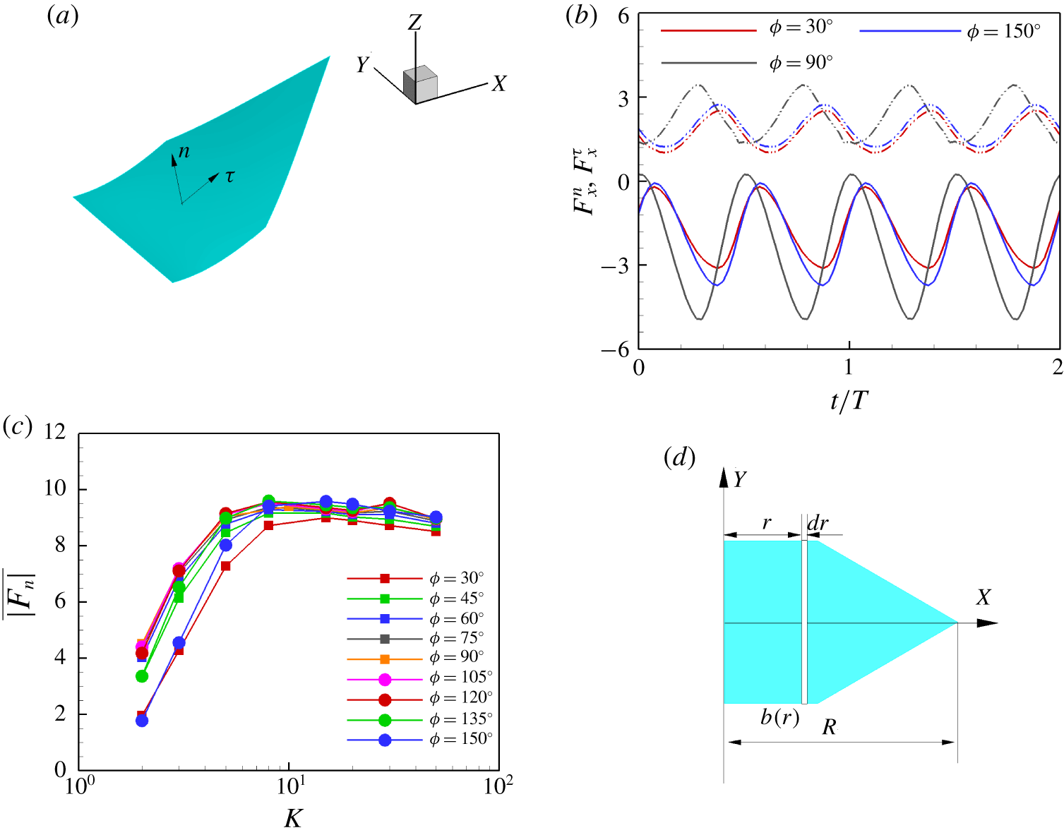
To better analyse the force acting on the plate, we decompose the force  $\boldsymbol{F}_{s}$ at each Lagrangian point into two parts: normal force
 $\boldsymbol{F}^{n}$ and tangential force
 $\boldsymbol{F}^{\unicode[STIX]{x1D70F}}$. These forces are defined as
 $$\begin{eqnarray}\displaystyle & \boldsymbol{F}^{n}=(\boldsymbol{F}_{s}\boldsymbol{\cdot }\boldsymbol{n})\boldsymbol{n}=(F_{x}^{n},F_{y}^{n},F_{z}^{n}), & \displaystyle\end{eqnarray}$$
 $$\begin{eqnarray}\displaystyle & \boldsymbol{F}^{\unicode[STIX]{x1D70F}}=\boldsymbol{F}_{s}-\boldsymbol{F}^{n}=(F_{x}^{\unicode[STIX]{x1D70F}},F_{y}^{\unicode[STIX]{x1D70F}},F_{z}^{\unicode[STIX]{x1D70F}}), & \displaystyle\end{eqnarray}$$
where  $\boldsymbol{n}$ and
 $\unicode[STIX]{x1D749}$ are the unit normal and tangential vectors, respectively, as shown in figure 18(a).
(a) The normal and tangential directions at a Lagrangian point on the plate. (b) The  $x$-component of
 $\boldsymbol{F}^{n}$ and
 $\boldsymbol{F}^{\unicode[STIX]{x1D70F}}$ for the plates with
 $K=3$. The solid and dashed lines represent the
 $x$-component of
 $\boldsymbol{F}^{n}$ and
 $\boldsymbol{F}^{\unicode[STIX]{x1D70F}}$, respectively. (c) The time-averaged absolute normal force integrated on the plates as a function of
 $K$. (d) A schematic diagram for the area moment, where
 $b(r)$ is the width of the plate in the spanwise direction at
 $X=r$.

For example,  $F_{x}^{n}$ and
 $F_{x}^{\unicode[STIX]{x1D70F}}$ during two flapping periods in the cases of
 $K=3$ are shown in figure 18(b). It is seen that the
 $x$-component normal forces (
 $F_{x}^{n}$) are almost all negative and the
 $x$-component tangential forces (
 $F_{x}^{\unicode[STIX]{x1D70F}}$) are all positive. Hence, the normal force contributes much to the thrust force and the tangential force produces drag in all cases with different trailing-edge shape. It is also noted that in all cases, the time average of the total horizontal force (
 $F_{x}^{n}+F_{x}^{\unicode[STIX]{x1D70F}}$) in a flapping period is zero. Meanwhile, we can see that at
 $K=3$, the mean value of
 $F_{x}^{n}$ of the square plate is much larger than those of the convex and concave plates. Correspondingly, we see that at
 $K=3$, the propulsive performance of the square plate is the best approximately.
Figure 18(c) shows the time-averaged absolute normal force integrated on the plates over several periods  $\overline{|\boldsymbol{F}^{n}|}$ as a function of
 $K$. We can see that
 $\overline{|\boldsymbol{F}^{n}|}$ increases with
 $K$ when
 $K<8$; this can be observed from the pressure contours of
 $K=3$ and 8 in figures 14 and 15, respectively. When
 $K>8$,
 $\overline{|\boldsymbol{F}^{n}|}$ almost reaches a plateau. It is noticed that, although in figure 17(c)
 $\unicode[STIX]{x1D703}/\unicode[STIX]{x1D6FC}$ decreases at
 $K\approx 5$,
 $F_{x}^{n}$ is still large enough because
 $\overline{|\boldsymbol{F}^{n}|}$ increases significantly from
 $K=3$ to
 $K=5$. On the other hand, when
 $K$ is large, although the normal force is large,
 $\unicode[STIX]{x1D703}/\unicode[STIX]{x1D6FC}$ tends to be zero and the normal force would not contribute much to the thrust. Hence, the propulsive performance reaches peak at
 $K\in [3,5]$.
However, it is possible that there is a dynamic similarity between these plates. We seek a rescaling law to reveal the inherent similarity between plates with different  $\unicode[STIX]{x1D719}$.
To quantify the effect of the plate shape on the propulsive performance, the area moments are used. According to the description of morphological parameters for insect wings (Ellington Reference Ellington1984), the  $k$th non-dimensional radius of the area moment is calculated as
 $$\begin{eqnarray}\displaystyle & \displaystyle \hat{r}_{k}=\left(\frac{S_{k}}{S_{0}R^{k}}\right)^{1/k}, & \displaystyle\end{eqnarray}$$
 $$\begin{eqnarray}\displaystyle & \displaystyle S_{k}=\int _{0}^{R}r^{k}b(r)\,\text{d}r, & \displaystyle\end{eqnarray}$$
where  $S_{k}$ is the
 $k$th area moment with
 $k=0,1,\ldots ,b(r)$ is the width of the plate in the spanwise direction at
 $X=r$ and
 $R$ is the maximal chord length of the plate. A schematic diagram of the area moment is shown in figure 18(d). The present geometric parameter of trailing-edge shape is in the range of statistical results for insect wings (Ellington Reference Ellington1984) and fish caudal fins (Lu, Yin & Tong Reference Lu, Yin and Tong2008), i.e.
 $\hat{r}_{1}\in (0.3,0.6)$.
According to the discussions above, the normal force dominates the propulsive performance of the plate. For the scaling law, it would be reasonable that the fluid force  $\unicode[STIX]{x1D70C}U_{ref}^{2}L^{2}$ in relevant parameters is replaced by the normal force. Therefore we introduce a dynamic parameter
 $\unicode[STIX]{x1D6EC}=\overline{|\boldsymbol{F}^{n}|}^{\prime }/\unicode[STIX]{x1D70C}U_{ref}^{2}L^{2}=\overline{|\boldsymbol{F}^{n}|}^{\prime }/2F_{ref}$ to represent the ratio of the normal force
 $\overline{|\boldsymbol{F}^{n}|}^{\prime }$ and the fluid force
 $\unicode[STIX]{x1D70C}U_{ref}^{2}L^{2}$, where
 $\overline{|\boldsymbol{F}^{n}|}^{\prime }$ is the corresponding dimensional quantity of
 $\overline{|\boldsymbol{F}^{n}|}$. Then
 $\unicode[STIX]{x1D6EC}$ is adopted to rescale the parameters
 $K$ and
 $U_{ref}$. As we know, the bending stiffness coefficient
 $K=EI/\unicode[STIX]{x1D70C}U_{ref}^{2}L^{3}$ demonstrates the ratio of elastic force (
 $EI/L$) and fluid force (
 $\unicode[STIX]{x1D70C}U_{ref}^{2}L^{2}$), then the bending rigidity is redefined as
 $K^{\prime }=EI/L/\overline{|\boldsymbol{F}^{n}|}^{\prime }=K/\unicode[STIX]{x1D6EC}$. Besides, to incorporate the effect of the geometric shape of the plate, the bending rigidity is further redefined as
 $K^{\ast }=K/(\unicode[STIX]{x1D6EC}/\hat{r}_{1})$. Meanwhile, the original characteristic speed
 $U_{ref}=\sqrt{2F_{ref}/\unicode[STIX]{x1D70C}L^{2}}$ should be redefined as
 $U_{ref}^{\ast }=\sqrt{\overline{|\boldsymbol{F}^{n}|}^{\prime }/\unicode[STIX]{x1D70C}L^{2}}=\sqrt{\unicode[STIX]{x1D6EC}}U_{ref}$. The rescaled propulsive velocity
 $U^{\ast }$ and efficiency
 $\unicode[STIX]{x1D702}^{\ast }$ (
 $\unicode[STIX]{x1D702}^{\ast }=\frac{1}{2}M{U^{\ast }}^{2}/W$) as functions of
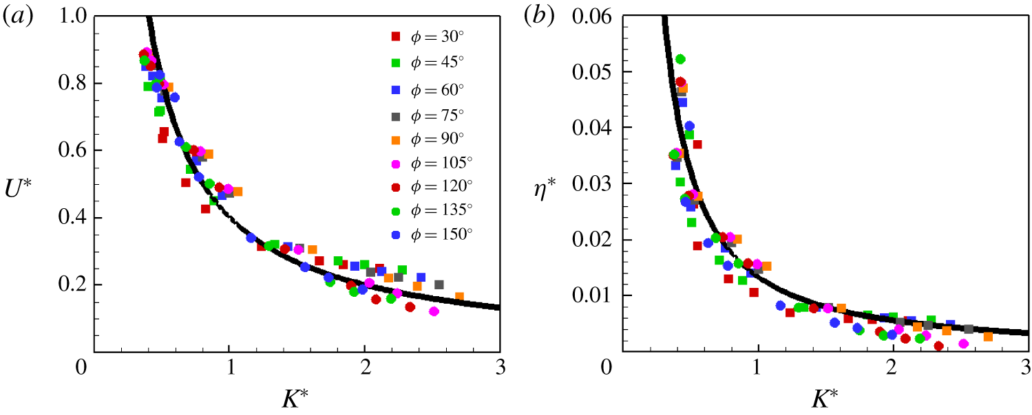
 $K^{\ast }$ are shown in figure 19(a,b). It can be seen that
 $U^{\ast }$ and
 $\unicode[STIX]{x1D702}^{\ast }$ for different trailing-edge shapes almost collapse into a single curve in figures 19(a) and 19(b), respectively. Both
 $U^{\ast }$ and
 $\unicode[STIX]{x1D702}^{\ast }$ decrease monotonically with
 $K^{\ast }$ for all shapes of plate. It seems that the
 $\unicode[STIX]{x1D719}$ effect is governed by the area moment. On the other hand, when
 $K^{\ast }$ is very large, the rescaled results deviate from the fitting curve (not shown). This can be explained as follows. Analysis in Vandenberghe et al. (Reference Vandenberghe, Zhang and Childress2004) has shown that when a rigid wing flaps up and down, the thrust force is mainly generated by the leading-edge vortex, which induces suction pressure. In other words, for a plate with large
 $K$, the normal force is not the key factor of the horizontal motion of plate. Hence, under this circumstance, the normal force replacing the fluid force
 $\unicode[STIX]{x1D70C}U_{ref}^{2}L$ may be not appropriate. It is also not expected that the rescaling using the normal force can achieve a very good result at larger
 $K$.
(a) Rescaled propulsive velocity and (b) rescaled propulsive efficiency of the plates as a function of the rescaled bending stiffness coefficient for different trailing-edge shapes. The black lines are fitting curves.

5 Conclusion
In order to investigate the impact of trailing-edge shape on the propulsive performance of plates, a series of numerical simulations are conducted at a moderate Reynolds number ( ${\sim}10^{2}$). The vortical structure, velocity fields, pressure and deformation of plates are analysed. We summarize the results as follows.
As the plates are very flexible, the propulsive speed  $U$ and efficiency
 $\unicode[STIX]{x1D702}$ of the plates first increase with the trailing-edge angle
 $\unicode[STIX]{x1D719}$, then decrease. Under this circumstance, the propulsive performance of the plate with
 $\unicode[STIX]{x1D719}\approx 90^{\circ }$ is superior to those of the concave and convex plates at the expense of larger input work. At moderate
 $K$,
 $U$ and
 $\unicode[STIX]{x1D702}$ of the plate increase monotonically with the trailing-edge angle and the convex plate is able to achieve the best performance. As the plate is relatively rigid,
 $U$ and
 $\unicode[STIX]{x1D702}$ decrease with
 $\unicode[STIX]{x1D719}$ until
 $\unicode[STIX]{x1D719}=120^{\circ }$, then increase. The convex plate seems to be the best in terms of propulsion performance.
The wake characteristics were analysed in terms of the vortical structures behind the plate and the time-averaged streamwise velocity field. At small and moderate  $K$, the wake behind the concave plate is composed of a chain of horseshoe-like structures. The wakes behind the square and convex plates usually consist of two set of vortex rings. The wake behind the plate is usually shorter in the cases with higher
 $K$. At higher
 $K$, there is a new kind of wake behind the convex plate, i.e. two-line vortex rings instead of only one line behind the trailing edge. The analyses of time-averaged streamwise velocity fields show that usually the jet behind the best plate is longer than those of the other plates. Meanwhile, the inclination angle of the jet may be small.
At large  $K$, the leading-edge vortex instead of the normal force plays an important role for the propulsion performance. We observed that the strength of the leading-edge vortex increases with
 $\unicode[STIX]{x1D719}$ until
 $\unicode[STIX]{x1D719}=120^{\circ }$. At
 $\unicode[STIX]{x1D719}\approx 120^{\circ }$, the leading-edge vortex is almost as strong as the trailing-edge vortex and the flow field around the plate is nearly symmetric. Therefore, the thrust force is small and the propulsion performance is the worst.
The pressure fields and deformation of the plates are analysed to estimate the force acting on the plate at small and moderate  $K$. The optimal phase lag of the trailing edge leads to the best propulsive performance. In addition, it is also observed that resonance can improve the propulsive performance of the plate. It is found that the thrust force is mainly contributed by the normal force. If
 $U$,
 $\unicode[STIX]{x1D702}$ and
 $K$ are rescaled by the normal force
 $\overline{|\boldsymbol{F}^{n}|}$ and the first area moment of the plate, the curves for different
 $\unicode[STIX]{x1D719}$ almost collapse into a single curve for
 $K\in (2,25)$. In other words, we found that only
 $\overline{|\boldsymbol{F}^{n}|}$ instead of the maximum or the averaged thrust force is able to achieve a good scaling. Hence, the scaling confirms that the normal force should be the characteristic fluid force at small or moderate
 $K$ and the
 $\unicode[STIX]{x1D719}$ effect is governed by the area moment. This is one of our contributions. Although the normal force is not an a priori quantity, we believe that the scaling here does help point the right way for developing an a priori scaling. The dynamic similarity provides a physical insight into the understanding of hydrodynamics in self-propulsion and the intrinsic relation to the geometric shape of the propeller of animals in nature.
Acknowledgements
This work was supported by Natural Science Foundation of China (NSFC) grant nos 11872064 and 11621202. H.H. is supported by NSFC grant no. 11772326.
Declaration of interests
The authors report no conflict of interest.