





1 Introduction
The fast ignition (FI)[ Reference Tabak, Hammer, Glinsky, Kruer, Wilks, Woodworth, Campbell, Perry and Mason 1 – Reference Gong, Habara, Sumioka, Yoshimoto, Hayashi, Kawazu, Otsuki, Matsumoto, Minami, Abe, Aizawa, Enmei, Fujita, Ikegami, Makiyama, Okazaki, Okida, Tsukamoto, Arikawa, Fujioka, Iwasa, Lee, Nagatomo, Shiraga, Yamanoi, Wei and Tanaka 6 ] scheme is a promising alternative approach to achieve inertial confinement fusion (ICF). In contrast to central ignition schemes[ Reference Nuckolls, Wood, Thiessen and Zimmerman 7 – Reference Abu-Shawareb, Acree, Adams, Adams, Addis, Aden, Adrian, Afeyan, Aggleton and Aghaian 14 ] of ICF, the FI scheme exploits MeV-level fast electrons generated by laser pulses of relativistic intensity to heat the core region of a pre-compressed target. The separation of heating process from the compression process relaxes the fuel assembly requirements[ Reference Tabak, Hammer, Glinsky, Kruer, Wilks, Woodworth, Campbell, Perry and Mason 1 , Reference Basov, Gus’Kov and Feokistov 2 ], offering the potential for high fusion gain with reduced laser energy. Nevertheless, theoretical studies indicate that the laser energy required for ignition remains of the order of several tens of kilojoules (kJ)[ Reference Atzeni 15 – Reference Bellei, Divol, Kemp, Key, Larson, Strozzi, Marinak, Tabak and Patel 17 ]. Moreover, both theoretical and experimental investigations have demonstrated that the energy conversion efficiency is relatively low, primarily due to limited laser–plasma interaction (LPI) efficiency[ Reference Kemp, Sentoku and Tabak 18 – Reference Fujioka, Johzaki, Arikawa, Zhang, Morace, Ikenouchi, Ozaki, Nagai, Abe, Kojima, Sakata, Inoue, Utsugi, Hattori, Hosoda, Lee, Shigemori, Hironaka, Sunahara, Sakagami, Mima, Fujimoto, Yamanoi, Norimatsu, Tokita, Nakata, Kawanaka, Jitsuno, Miyanaga, Nakai, Nishimura, Shiraga, Nagatomo and Azechi 22 ] and the divergent motion of fast electrons during transport[ Reference Sheng, Sentoku, Mima, Zhang, Yu and Meyer-ter-Vehn 23 – Reference Shiraga, Fujioka, Nakai, Watari, Nakamura, Arikawa, Hosoda, Nagai, Koga, Kikuchi, Ishii, Sogo, Shigemori, Nishimura, Zhang, Tanabe, Ohira, Fujii, Namimoto, Sakawa, Maegawa, Ozaki, Tanaka, Habara, Iwawaki, Shimada, Nagatomo, Johzaki, Sunahara, Murakami, Sakagami, Taguchi, Norimatsu, Homma, Fujimoto, Iwamoto, Miyanaga, Kawanaka, Jitsuno, Nakata, Tsubakimoto, Morio, Kawasaki, Sawai, Tsuji, Murakami, Kanabe, Kondo, Sarukura, Shimizu, Mima and Azechi 26 ]. Improving the generation and transport efficiency of fast electrons therefore remains a central challenge for FI.
Recent advances in multi-petawatt laser facilities, including ARC at NIF in the United States[
Reference Moses, Boyd, Remington, Keane and Al-Ayat
27
], the Vulcan system in the UK[
Reference Hernandez-Gomez, Blake, Chekhlov, Clarke, Dunne, Galimberti, Hancock, Heathcote, Holligan, Lyachev, Matousek, Musgrave, Neely, Norreys, Ross, Tang, Winstone, Wyborn and Collier
28
], LFEX facility in Japan[
Reference Azechi, Mima, Fujimoto, Fujioka, Homma, Isobe, Iwamoto, Jitsuno, Johzaki, Kodama, Koga, Kondo, Kawanaka, Mito, Miyanaga, Motojima, Murakami, Nagatomo, Nagai, Nakai, Nakamura, Nakamura, Nakazato, Nakao, Nishihara, Nishimura, Norimatsu, Ozaki, Sakagami, Sakawa, Sarukura, Shigemori, Shimizu, Shiraga, Sunahara, Taguchi, Tanaka and Tsubakimoto
29
] and the SG-II-U facility in China, provide capability to deliver laser energy from kJ to tens of kJ within picoseconds (ps). In these facilities, multiple laser beams are typically arranged with different incident angles. Previous studies have shown that the interaction of two laser pulses can enhance fast-electron generation, with an optimal crossing angle of about 16°–20°, identified by scanning from
$0{}^{\circ}$
 to
$30{}^{\circ}$
 [
Reference Zhou, Wang, Li and Zhang
30
]. However, in practical multi-beam geometries the crossing angle can be substantially larger. For example, the next-generation high-energy laser facility SG-X, under construction in Shanghai and designed for the double-cone ignition (DCI) scheme[
Reference Zhang, Wang, Yang, Wu, Ma, Jiao, Zhang, Wu, Yuan, Li and Zhu
31
–
Reference Dai, Gu, Fang, Zhang, Zhang, Dong, Zhang, Yuan, Li and Zhang
34
], will deliver 12 ps laser beams, with an angle between the two outermost beams approaching
$60{}^{\circ}$
 . Since existing optimizations largely focus on small-angle configurations, it is crucial to assess and optimize fast-electron generation in such a large-angle regime.
Various approaches have been proposed to enhance the energy conversion efficiency of fast electrons. These approaches are implemented either by adjusting the laser pulse parameters[
Reference Zhou, Wang, Li and Zhang
30
,
Reference Ping, Shepherd, Lasinski, Tabak, Chen, Chung, Fournier, Hansen, Kemp, Liedahl, Widmann, Wilks, Rozmus and Sherlock
35
,
Reference Zhang, Wang, Li and Zhang
36
] or target parameters[
Reference Kemp, Sentoku and Tabak
18
,
Reference Mishra, Sentoku and Kemp
19
,
Reference Culfa, Tallents, Rossall, Wagenaars, Ridgers, Murphy, Dance, Gray, McKenna, Brown, James, Hoarty, Booth, Robinson, Lancaster, Pikuz, Faenov, Kampfer, Schulze, Uschmann and Woolsey
37
] to enhance the coupling efficiency of LPI or by applying an external strong magnetic field of kilo-tesla to confine the divergent motion of fast electrons[
Reference Wang, Gibbon, Sheng and Li
38
–
Reference Sakata, Lee, Morita, Johzaki, Sawada, Iwasa, Matsuo, Law, Yao, Hata, Sunahara, Kojima, Abe, Kishimoto, Syuhada, Shiroto, Morace, Yogo, Iwata, Nakai, Sakagami, Ozaki, Yamanoi, Norimatsu, Nakata, Tokita, Miyanaga, Kawanaka, Shiraga, Mima, Nishimura, Bailly-Grandvaux, Santos, Nagatomo, Azechi, Kodama, Arikawa, Sentoku and Fujioka
41
]. In the present work, we focus on the interaction of two laser pulses with a large crossing angle up to
$60{}^{\circ}$
 and analyze the plasma surface structures formed by their interference. We show that the interference-induced surface modulation becomes more susceptible to laser filamentation[
Reference Shvets and Wurtele
42
–
Reference Najmudin, Krushelnick, Tatarakis, Clark, Danson, Malka, Neely, Santala and Dangor
44
] at large crossing angles, which degrades LPI efficiency and fast-electron generation. Based on this understanding, we propose to shift the crossing point of the two laser pulses from the vacuum–plasma boundary into the target interior. This geometric adjustment enhances the pulse overlap near the critical-density region and promotes the formation of a more stable plasma surface structure, thereby improving fast-electron generation. The optimal crossing point is found to be close to the laser hole boring depth, approximately
$15\;\mu \mathrm{m}$
 in our case. We further investigate the impact of the strength of an external uniform magnetic field on fast-electron transport under this optimized configuration. We confirm the validity of the magnetic-field confinement on fast electrons and obtain an appropriate magnetic-field strength that can be both effective and achievable in experiments.
This paper is organized as follows. In Sections 2–4, we present particle-in-cell (PIC) simulation results on fast-electron generation and transport driven by the interaction of two picosecond laser pulses with a solid target. In Section 2, we show that both laser absorption and fast-electron generation decrease at a large crossing angle of
$60{}^{\circ}$
 compared with the case of an optimized angle around
$20{}^{\circ}$
 . This decrease can be attributed to the change in the plasma surface structure and, hence, we propose to shift the crossing point of the two laser pulses. In Section 3, we confirm this approach and show that fast-electron generation can be substantially enhanced by shifting the crossing point from the vacuum–plasma boundary into the plasma interior. We identify an optimal crossing point, which also benefits fast-electron transport. Next, we examine the magnetic-field guiding of fast-electron transport in the optimized geometry in Section 4. Finally, a brief summary is presented in Section 5.
2 Crossing-angle dependence of fast-electron generation
We carry out a series of two-dimensional (2D) PIC simulations with the KLAPS code[
Reference Wang, Gibbon, Sheng and Li
45
], where absorption boundaries are taken in both directions of
$x$
 and
$y$
 and the fourth-order current calculation is used to reduce the numerical noise[
Reference Esirkepov
46
]. In our simulations, two laser pulses are symmetrically incident at the plasma target under different spatial configurations. Each laser pulse has the electric field expressed as
${E}_y={a}_0\exp \left(-{y}^2/{r}_0^2\right)\sin \left(\pi t/{\tau}_0\right)\sin \left(2\pi t/{\lambda}_\mathrm{L}\right)$
 , where
${a}_0=6$
 corresponds to a peak intensity of
$5\times {10}^{19}\;\mathrm{W}/{\mathrm{cm}}^2$
 , and
${r}_0=10\;\mu \mathrm{m}$
 ,
${\tau}_0=1\;\mathrm{ps}$
 and
${\lambda}_\mathrm{L}=1\;\mu \mathrm{m}$
 are its spot size, duration and wavelength, respectively. The plasma consists of electrons and Au ions with a static ionization of
$Z=10$
 . Both electrons and ions are initialized with Maxwell–Boltzmann momentum distributions at a temperature of
${T}_\mathrm{e}={T}_\mathrm{i}=500\;\mathrm{eV}$
 . The size of the simulation box is
$80\;\mu \mathrm{m}\times 96\;\mu \mathrm{m}$
 in the
$x\times y$
 directions with
$2560\times 3072$
 cells. Each cell contains
$36$
 macroparticles for each species. A vacuum region is located in the range
$-25\;\mu \mathrm{m}<x\leqslant 0$
 , a preplasma with an exponential ramp from
$0.01{n}_\mathrm{c}$
 to
$100{n}_\mathrm{c}$
 and a scale length of
$2\;\mu \mathrm{m}$
 is imposed within
$0<x\leqslant 18.42\;\mu \mathrm{m}$
 and a uniform plasma with a density of
$100{n}_\mathrm{c}$
 is followed at
$x>18.42\;\mu \mathrm{m}$
 , where
${n}_\mathrm{c}=1.1\times {10}^{21}\;{\mathrm{cm}}^{-3}$
 is the plasma critical density.
To investigate the effects of the laser pulses configurations on the fast-electron generation, we adopt two laser configurations. Case I: the two laser pulses cross at the vacuum–plasma boundary
${x}_\mathrm{c}=0$
 , and the crossing angle
$\theta$
 is varied from
$0{}^{\circ}$
 to
$60{}^{\circ}$
 to examine the impact of the crossing angle on fast-electron generation. Case II: the crossing angle is fixed at
$\theta =60{}^{\circ}$
 , approaching the angle between the two outermost ps beams at SG-X, while the crossing point of the two pulses is scanned from the vacuum–plasma boundary toward the target interior. In both cases, the longitudinal distance from each laser injection point to the vacuum–plasma boundary is kept constant at
$12\;\mu \mathrm{m}$
 .
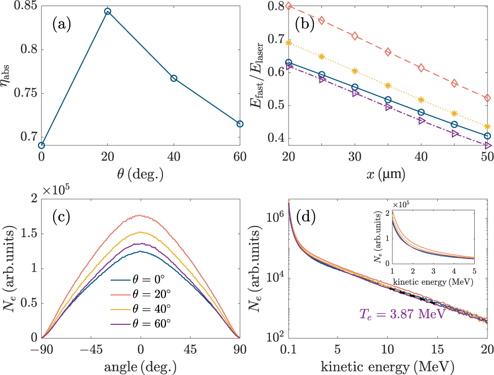
We first investigate the impact of the laser crossing angle on the fast-electron generation. In our PIC simulations, the crossing angles are taken as
$\theta =0{}^{\circ}$
 ,
$20{}^{\circ}$
 ,
$40{}^{\circ}$
 and
$60{}^{\circ}$
 , respectively. The laser absorption rate
${\eta}_{\mathrm{abs}}$
 , shown in Figure 1(a), is evaluated as
$1-\left({E}_{\mathrm{ref}}+{E}_{\mathrm{tra}}+{E}_{\mathrm{sca}}\right)/{E}_{\mathrm{laser}}$
 , where
${E}_{\mathrm{ref}}$
 ,
${E}_{\mathrm{tra}}$
 ,
${E}_{\mathrm{sca}}$
 and
${E}_{\mathrm{laser}}$
 denote the reflected, transmitted, scattered and incident laser energy, respectively. It is clear that
${\eta}_{\mathrm{abs}}$
 reaches its maximum at
$\theta =20{}^{\circ}$
 and decreases for larger crossing angles. This trend is consistent with Ref. [Reference Zhou, Wang, Li and Zhang30] and indicates that the laser–plasma coupling becomes less efficient at
$\theta =60{}^{\circ}$
 . Figure 1(b) shows the total energy of forward fast electrons
${E}_{\mathrm{fast}}$
 collected at each observing section from
$x=20\;\mu \mathrm{m}$
 to
$x=50\;\mu \mathrm{m}$
 , where the energy is normalized by the incident laser energy
${E}_{\mathrm{laser}}$
 . Consistent with the reduction in laser absorption,
${E}_{\mathrm{fast}}$
 decreases with
$\theta$
 at all observing sections. The angle and energy spectra of fast electrons further reflect this trend. As is shown in Figure 1(c), compared with the
$\theta =20{}^{\circ}$
 case, the angle spectra at
$x=20\;\mu \mathrm{m}$
 exhibit generally lower amplitude for
$\theta =60{}^{\circ}$
 , implying a reduced number of forward fast electrons. Similarly, the energy spectra in Figure 1(d) show fewer fast electrons over a broad energy range for
$\theta =60{}^{\circ}$
 , including the
$1-5\;\mathrm{MeV}$
 interval, which is particularly relevant for core heating in FI[
Reference Betti, Solodov, Delettrez and Zhou
47
–
Reference Craxton, Anderson, Boehly, Goncharov, Harding, Knauer, McCrory, McKenty, Meyerhofer, Myatt, Schmitt, Sethian, Short, Skupsky, Theobald, Kruer, Tanaka, Betti, Collins, Delettrez, Hu, Marozas, Maximov, Michel, Radha, Regan, Sangster, Seka, Solodov, Soures, Stoeckl and Zuegel
49
]. These results demonstrate that large crossing angles, although unavoidable in practical multi-beam configurations, are intrinsically unfavorable for fast-electron generation, thereby motivating the crossing-point optimization discussed in the following section.
(a) Laser absorption rate as a function of
$\theta$
 and (b) the total energy of fast electrons passing through each observing section from
${x=20\;\mu \mathrm{m}}$
 to
$x=50\;\mu \mathrm{m}$
 , as well as (c) angle spectra and (d) energy spectra of fast electrons passing through the
$x=20\;\mu \mathrm{m}$
 section, where the crossing points are taken as
${x}_\mathrm{c}=0$
 . In each plot of (b)–(d), four curves correspond to
$\theta =0{}^{\circ}$
 (blue curve),
$\theta =20{}^{\circ}$
 (orange curve),
$\theta =40{}^{\circ}$
 (yellow curve) and
$\theta =60{}^{\circ}$
 (purple curve), respectively.

Figure 1 Long description
Panel a is a line graph of eta sub abs versus theta in degrees. The x-axis ranges from 0 to 60 and the y-axis from 0.7 to 0.85. The curve peaks at theta equals 20 with a value of approximately 0.84 before decreasing.
Panel b shows the ratio E sub fast over E sub laser versus x in mu m from 20 to 50. Four downward-sloping linear trends are shown for theta values 0, 20, 40, and 60 degrees. The highest energy ratio is for theta equals 20 degrees (red diamonds) and the lowest for theta equals 60 degrees (purple triangles).
Panel c displays N sub e in arbitrary units versus angle in degrees from negative 90 to 90. It shows four bell-shaped curves centered at 0 degrees. The peak intensity is highest for theta equals 20 degrees (red) and lowest for theta equals 0 degrees (blue).
Panel d is a semi-log plot of N sub e versus kinetic energy in M e V from 0.1 to 20. The curves decay exponentially. An inset shows the same data on a linear scale for kinetic energy from 1 to 5 M e V. A text label indicates T sub e equals 3.87 M e V for the purple curve.
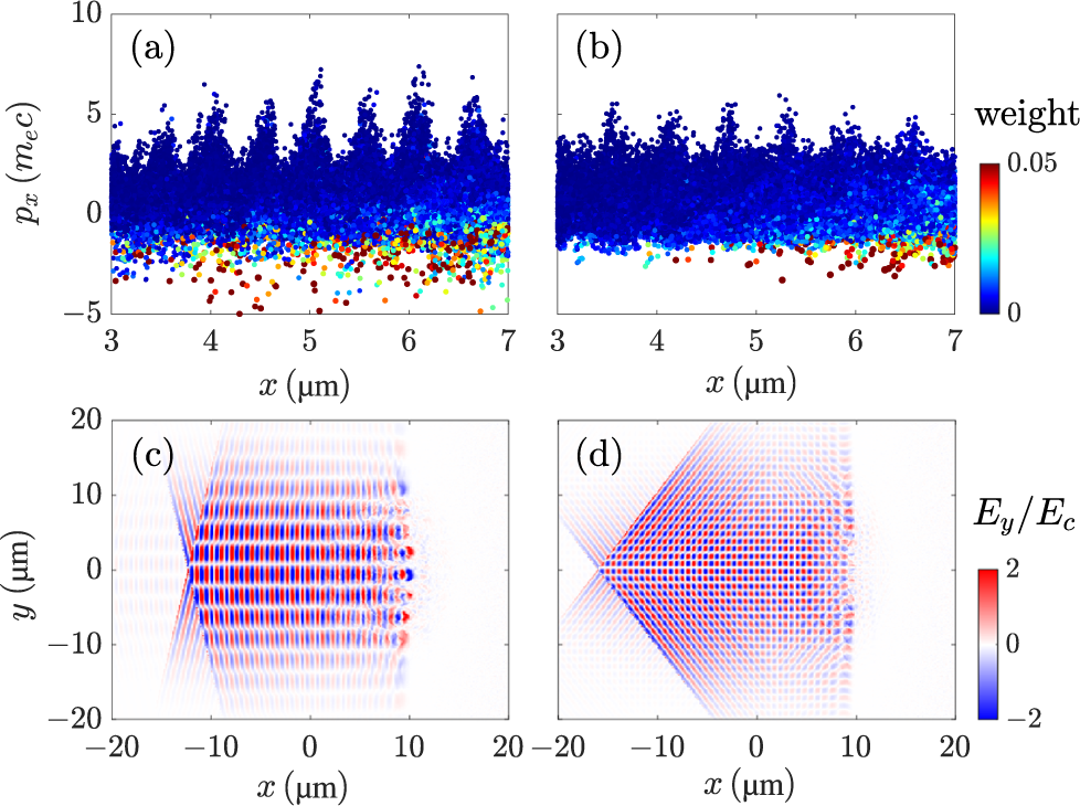
Figures 2(a) and 2(b) present the phase spaces of fast electrons at
$t=0.13\;\mathrm{ps}$
 for
$\theta =20{}^{\circ}$
 and
$\theta =60{}^{\circ}$
 , respectively, where
${p}_x$
 denotes the electron longitudinal momentum. It is quite clear that the electron bunches exhibit several periodic peaks with a spacing of
$0.5{\lambda}_\mathrm{L}$
 for
$\theta =20{}^{\circ}$
 . Such a spacing is characteristic of electron acceleration driven by the
$2{\omega}_\mathrm{L}$
 component of the Lorentz force in relativistic LPIs and is consistent with
$\mathbf{J}\times \mathbf{B}$
 heating[
Reference Kruer and Estabrook
50
,
Reference Wilks, Kruer, Tabak and Langdon
51
]. Meanwhile, we notice that the fast-electron temperature for the
$\theta =60{}^{\circ}$
 case is
${T}_\mathrm{e}=3.87\;\mathrm{MeV}$
 , as shown in Figure 1(d), which is close to the ponderomotive scaling
${T}_\mathrm{e}=\left(\gamma -1\right){m}_\mathrm{e}{c}^2=3.88\;\mathrm{MeV}$
 , where
$\gamma ={\left(1+2I{\lambda}_\mathrm{L}^2/1.37\times {10}^{18}\;{\mu \mathrm{m}}^2\;\mathrm{W}/{\mathrm{cm}}^2\right)}^{1/2}$
 [
Reference Cui, Wang, Sheng, Li and Zhang
21
,
Reference Wilks, Kruer, Tabak and Langdon
51
]. This agreement indicates that
$\mathbf{J}\times \mathbf{B}$
 heating remains the dominant acceleration mechanism under both angle configurations. To analyze the reduced acceleration efficiency at large crossing angles, we compare the laser electric field
${E}_y$
 at
$t=0.13\;\mathrm{ps}$
 with the
$\theta =20{}^{\circ}$
 and
$\theta =60{}^{\circ}$
 cases, shown in Figures 2(c) and 2(d). For
$\theta =60{}^{\circ}$
 , the interference fringes become more oblique relative to the
$x$
 -direction and extend over a broader transverse region. As a result, the accelerating structure along the
$+x$
 direction becomes less coherent, leading to a smaller longitudinal momentum gain during each acceleration cycle. Consequently, fewer electrons are accumulated in each bunch and the peak values of
${p}_x$
 are reduced, in agreement with the phase space feature in Figure 2(b).
Phase spaces of fast electrons (top row) and normalized laser electric fields (bottom row) at
$t=0.13\;\mathrm{ps}$
 , where
${E}_\mathrm{c}={m}_\mathrm{e}c{\omega}_\mathrm{L}/e$
 . The angles between the two laser pulses are
$\theta =20{}^{\circ}$
 in (a) and (c) and
$\theta =60{}^{\circ}$
 in (b) and (d).

Figure 2 Long description
The top row contains two scatter plots labeled a and b. The x-axis represents position x in micrometers from 3 to 7. The y-axis represents momentum p sub x in units of m sub e c from minus 5 to 10. A color scale to the right indicates weight from 0 (blue) to 0.05 (red). Panel a, representing theta equals 20 degrees, shows seven distinct vertical peaks of high-density blue particles rising to p sub x equals 7, with scattered higher-weight red and yellow particles below the p sub x equals 0 line. Panel b, representing theta equals 60 degrees, shows similar but shorter and more compressed peaks reaching only p sub x equals 5. The bottom row contains two heat maps labeled c and d. The x-axis represents x in micrometers from minus 20 to 20, and the y-axis represents y in micrometers from minus 20 to 20. A color scale to the right indicates normalized electric field E sub y all over E sub c from minus 2 (blue) to 2 (red). Panel c shows a horizontal interference pattern concentrated along the y equals 0 axis. Panel d shows a wider, diamond-shaped interference pattern extending further along the y-axis.
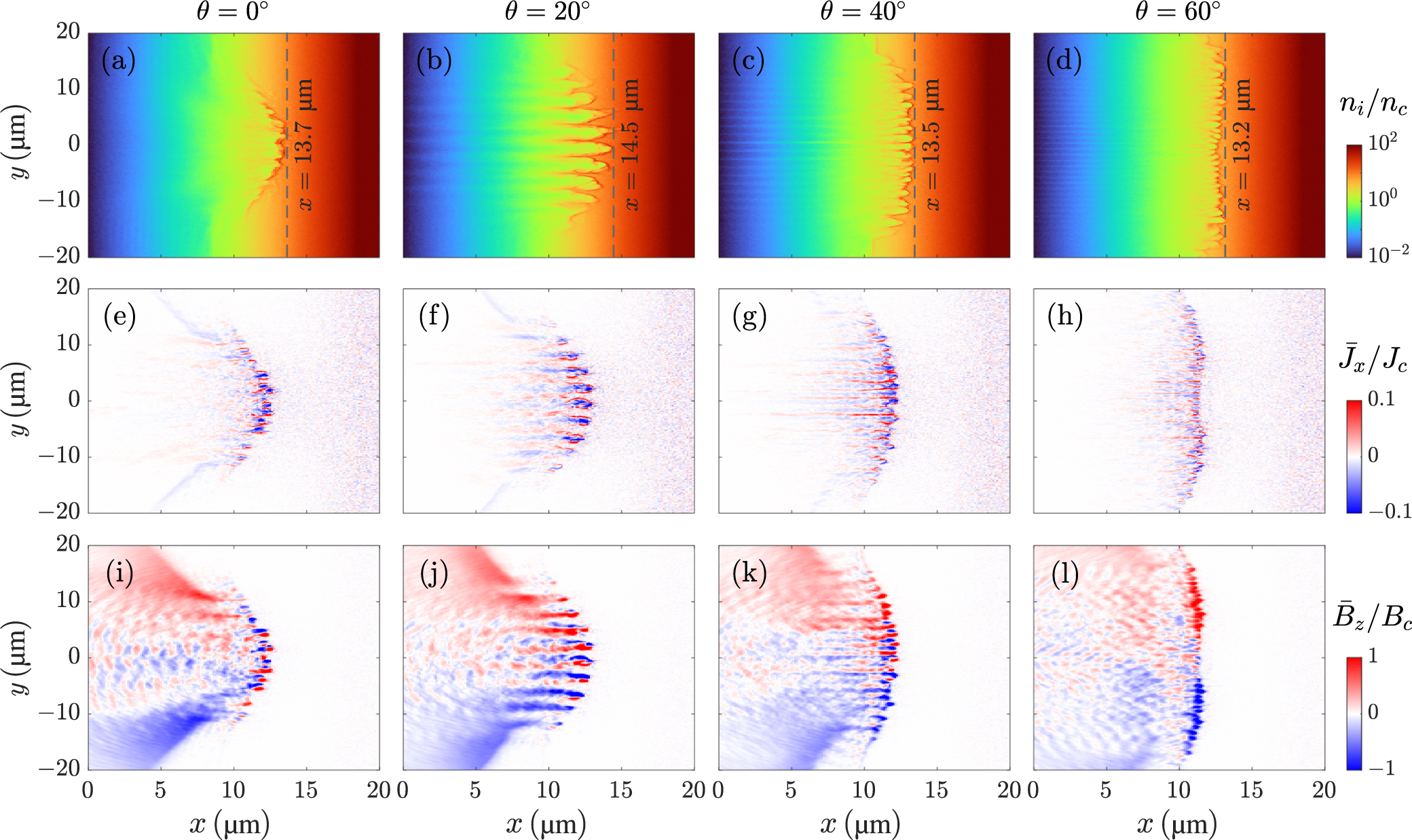
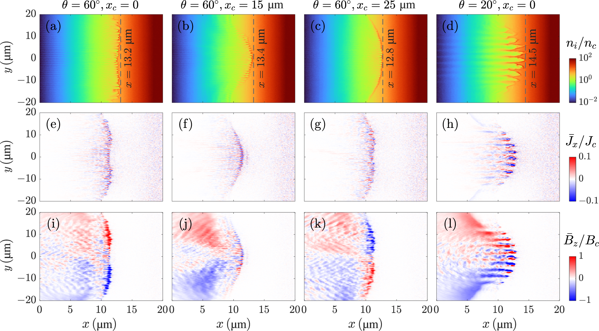
Figures 3(a)–3(d) show the ion density distributions
${n}_\mathrm{i}$
 at
$t=0.6\;\mathrm{ps}$
 . Here, we use dashed lines to mark the maximum penetration depth associated with laser hole boring. Among the four cases, the hole boring depth of
$x=13.2\;\mu \mathrm{m}$
 for
$\theta =60{}^{\circ}$
 is the smallest, indicating reduced laser–plasma coupling and a less efficient hole boring process at this large crossing angle. The plasma surface structure also changes significantly with the crossing angle. For
$\theta =0{}^{\circ}$
 , the surface remains relatively smooth with an approximately Gaussian transverse profile (see Figure 3(a)), whereas a clear periodic surface modulation appears for
$\theta =20{}^{\circ}$
 (see Figure 3(b)). In contrast, the surface becomes noticeably irregular for
$\theta =60{}^{\circ}$
 (see Figure 3(d)), consistent with the disruption of an interference-driven periodic structure by laser filamentation. For two laser pulses’ interference, the surface modulation period is
$T=\left({\lambda}_\mathrm{L}/2\right)/\sin \left(\theta /2\right)$
 , yielding
$T=1\;\mu \mathrm{m}$
 for
$\theta =60{}^{\circ}$
 , which is comparable to the laser wavelength. Such short-scale structures are more susceptible to perturbations in density and laser intensity, which can be amplified by the ponderomotive force and promote filamentation. The resulting loss of surface regularity reduces the laser hole boring process.
Snapshots of ion density
${n}_\mathrm{i}$
 (first row) at
$t=0.6\;\mathrm{ps}$
 , normalized electron current density
${\overline{J}}_x$
 (second row) and normalized self-generated magnetic field
${\overline{B}}_z$
 (third row) at
$t=0.27\;\mathrm{ps}$
 , where
${n}_\mathrm{c}={m}_\mathrm{e}{\omega}_\mathrm{L}^2/4\pi {e}^2$
 ,
${J}_\mathrm{c}={en}_\mathrm{c}c$
 and
${B}_\mathrm{c}={m}_\mathrm{e}c{\omega}_\mathrm{L}/e$
 . The first to fourth columns correspond to
$\theta =0{}^{\circ}$
 ,
$\theta =20{}^{\circ}$
 ,
$\theta =40{}^{\circ}$
 and
$\theta =60{}^{\circ}$
 , respectively.

Figure 3 Long description
The grid is organized into three rows. All panels share an x-axis from 0 to 20 micrometers and a y-axis from negative 20 to 20 micrometers.
* Top Row (Panels a through d): Displays ion density n sub i over n sub c at time t equals 0.6 picoseconds. A color scale on the right ranges from 10 super negative 2 (blue) to 10 super 2 (dark red). As theta increases, the plasma surface changes from a relatively smooth profile at 0 degrees to a periodic modulation at 20 degrees and a more irregular structure at 60 degrees. Vertical dashed lines mark the front position, decreasing from x equals 13.7 micrometers at 0 degrees to x equals 13.2 micrometers at 60 degrees.
* Middle Row (Panels e through h): Displays normalized electron current density J bar sub x over J sub c at time t equals 0.27 picoseconds. The color scale ranges from negative 0.1 (blue) to 0.1 (red). At 0 degrees, the current is concentrated in a central filamentary structure. As theta increases, the filaments become more numerous, smaller, and more evenly distributed along the y-axis.
* Bottom Row (Panels i through l): Displays normalized self-generated magnetic field B bar sub z over B sub c at time t equals 0.27 picoseconds. The color scale ranges from negative 1 (blue) to 1 (red). At 0 degrees, there is a clear dipolar structure with red on top and blue on bottom. As theta increases to 60 degrees, the magnetic field patterns become more fragmented and oscillatory, showing smaller-scale alternating red and blue regions along the expansion front.
This behavior is further reflected in the normalized current density distributions
${\overline{J}}_x$
 shown in Figures 3(e)–3(h) and magnetic-field distributions
${\overline{B}}_z$
 shown in Figures 3(i)–3(l). These quantities are averaged over one laser field period and evaluated at
$t=0.27\;\mathrm{ps}$
 . It is clear that the value of
${\overline{J}}_x$
 decreases as
$\theta$
 increases from
$20{}^{\circ}$
 to
$60{}^{\circ}$
 , indicating a weaker longitudinal fast-electron current. This trend is consistent with the reduced longitudinal momentum gain shown in the phase space distribution in Figure 2(b). A weaker longitudinal electron current naturally leads to a weaker self-generated magnetic field, explaining the reduced
${\overline{B}}_z$
 observed in Figure 3(l).
The shorter hole boring depth, weaker field strength and loss of surface regularity at
$\theta =60{}^{\circ}$
 together suggest that the filamentation plays a detrimental role in fast-electron generation at large crossing angles. Since such large-angle configurations are often unavoidable in multi-beam, high-energy laser systems, it is necessary to identify strategies to mitigate this effect. Motivated by the above observations, we propose to shift the laser pulse crossing point
${x}_\mathrm{c}$
 from the vacuum–plasma boundary into the target along the
$+x$
 direction, which is also the simulation we present in Section 3. This adjustment moves the interference region closer to the plasma critical-density zone and allows the surface modulation to form in the region where LPI is strongest, thereby reducing the growth of filamentation and improving fast-electron generation efficiency even at large crossing angles.
3 Optimization of fast-electron generation via crossing-point shifting
As discussed in Section 2, the location of the laser pulse crossing point is expected to influence both the strength of LPIs and the development of laser–plasma instabilities. In this section, we fix the crossing angle at
$\theta =60{}^{\circ}$
 , and shift the crossing point along the
$+x$
 direction from
${x}_\mathrm{c}=0$
 to
${x}_\mathrm{c}=25\;\mu \mathrm{m}$
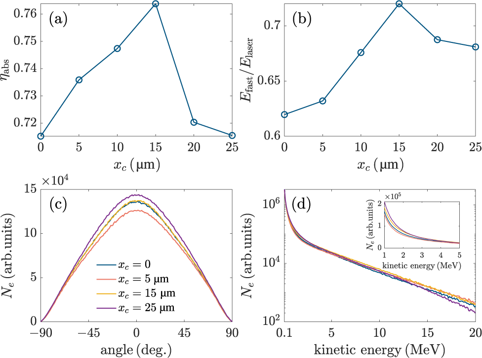
 . Figures 4(a) and 4(b) show the laser absorption rate
${\eta}_{\mathrm{abs}}$
 and total energy of forward fast electrons
${E}_{\mathrm{fast}}$
 collected at the observing section
$x=20\;\mu \mathrm{m}$
 . Both quantities increase as
${x}_\mathrm{c}$
 is shifted inward from the vacuum–plasma boundary, reach their maxima at
${x}_\mathrm{c}=15\;\mu \mathrm{m}$
 , and then decrease for larger
${x}_\mathrm{c}$
 . The simultaneous variation of
${\eta}_{\mathrm{abs}}$
 and
${E}_{\mathrm{fast}}$
 indicates that inward shifting of
${x}_\mathrm{c}$
 can effectively enhance laser–plasma coupling and fast-electron generation even under the unfavorable large-angle configuration. The optimal value
${x}_\mathrm{c}=15\;\mu \mathrm{m}$
 is closely related to the laser hole boring depth. For the present laser intensity of
$5\times {10}^{19}\;\mathrm{W}/{\mathrm{cm}}^2$
 , the plasma density that dual pulses can penetrate is
$\gamma {n}_\mathrm{c}=8.60{n}_\mathrm{c}$
 [
Reference Kaw and Dawson
52
], which corresponds to
$x=13.51\;\mu \mathrm{m}$
 in the initial plasma density profile. During the interaction, the density modulation induced by laser hole boring pushes the effective interaction front slightly deeper, to around
$x\simeq 14\;\mu \mathrm{m}$
 , consistent with the density distributions shown in Figures 3(a) and 3(b). Placing
${x}_\mathrm{c}$
 near this region enhances the pulse overlap where LPI is strongest and promotes a more regular plasma surface, leading to more efficient fast-electron generation, as reflected in the angle spectra in Figure 4(c) and the energy spectra in Figure 4(d). The slight offset between the optimal
${x}_\mathrm{c}$
 and the estimated penetration depth is expected, because the effective overlap region and surface stability depend on the dynamic plasma response rather than on the initial density profile alone.
(a) Laser absorption rate and (b) total energy as a function of
${x}_\mathrm{c}$
 , and (c) angle spectra and (d) energy spectra of fast electrons passing through the
$x=20\;\mu \mathrm{m}$
 section, where the crossing angle is taken as
$\theta =60{}^{\circ}$
 . In plots (c) and (d), four curves correspond to
${x}_\mathrm{c}=0$
 (blue curve),
${x}_\mathrm{c}=5\;\mu \mathrm{m}$
 (orange curve),
${x}_\mathrm{c}=15\;\mu \mathrm{m}$
 (yellow curve) and
${x}_\mathrm{c}=25\;\mu \mathrm{m}$
 (purple curve), respectively.

Figure 4 Long description
Panel a is a line graph of laser absorption eta sub abs versus x sub c in micrometers. The curve increases from 0.715 at x sub c equals 0 to a peak of 0.764 at x sub c equals 15, then drops sharply to 0.715 at x sub c equals 25.
Panel b is a line graph of the ratio E sub fast all over E sub laser versus x sub c. It follows a similar trend to panel a, rising from 0.62 at x sub c equals 0 to a peak of 0.72 at x sub c equals 15, before decreasing to 0.68 at x sub c equals 25.
Panel c is a line graph of electron count N sub e in arbitrary units versus angle in degrees, ranging from minus 90 to 90. Four bell-shaped curves peak at 0 degrees. The purple curve for x sub c equals 25 micrometers has the highest peak at approximately 1.4 times 10 super 4, followed by yellow (x sub c equals 15), blue (x sub c equals 0), and orange (x sub c equals 5).
Panel d is a semi-logarithmic line graph of N sub e versus kinetic energy in M e V, ranging from 0.1 to 20. The y-axis is logarithmic from 10 super 2 to 10 super 6. All four curves decay exponentially. An inset graph shows the low-energy region from 1 to 5 M e V on a linear scale, where the purple curve remains highest and the orange curve lowest.
For larger crossing points, for example,
${x}_\mathrm{c}\geqslant 20\;\mu \mathrm{m}$
 , both
${\eta}_{\mathrm{abs}}$
 and
${E}_{\mathrm{fast}}$
 decrease, while the total number of fast electrons continues to increase and reaches its maximum at
${x}_\mathrm{c}=25\;\mu \mathrm{m}$
 (see Figure 4(c)). In this case, the nominal crossing point lies deeper than the effective laser penetration region. Fast electrons are still mainly generated near the hole boring front, while the two laser axes are more separated there, reducing the pulse overlap and fringe contrast near the main acceleration region. As a result, the two-pulse enhancement of the longitudinal ponderomotive acceleration becomes weaker. Although electrons can still be heated over a broader but less coherent interaction region, their acceleration to higher energies becomes less efficient. This leads to an increased number of low-energy fast electrons but a reduced population of
$10-20\;\mathrm{MeV}$
 fast electrons for
${x}_\mathrm{c}=25\;\mu \mathrm{m}$
 , as shown in Figure 4(d).
To clarify the physical origin of this optimal crossing point, we further examine the plasma surface structure and associated current density and magnetic-field distributions. Figures 5(a)–5(c) present the ion density distributions for
${x}_\mathrm{c}=0$
 ,
$15\;\mu \mathrm{m}$
 and
$25\;\mu \mathrm{m}$
 at
$\theta =60{}^{\circ}$
 , while Figure 5(d) presents the optimal-angle case of
$\theta =20{}^{\circ}$
 as a benchmark. For
$\theta =60{}^{\circ}$
 cases, the plasma surface structure evolves systematically as
${x}_\mathrm{c}$
 is shifted inward. At
${x}_\mathrm{c}=0$
 , the plasma surface exhibits irregular structures associated with strong filamentation. When the crossing point is shifted to
${x}_\mathrm{c}=15\;\mu \mathrm{m}$
 , the surface becomes significantly smoother and approaches a Gaussian-like transverse profile, accompanied by a deeper laser hole boring depth. This behavior suggests more effective laser–plasma coupling and reduced filamentation. For
${x}_\mathrm{c}=25\;\mu \mathrm{m}$
 , although the surface remains relatively smooth, the hole boring depth decreases again, implying a weaker overall interaction strength. The corresponding normalized current density
${\overline{J}}_x$
 and self-generated magnetic field
${\overline{B}}_z$
 are shown in Figures 5(e)–5(h) and 5(i)–5(l), respectively. For
${x}_\mathrm{c}=15\;\mu \mathrm{m}$
 , both
${\overline{J}}_x$
 and
${\overline{B}}_z$
 exhibit transverse profiles closely following the ion density distribution, with pronounced peaks near
$y=0$
 . This correlation reflects efficient hole boring driven by the forward fast-electron current and the associated self-generated magnetic field. These results support that placing the
${x}_\mathrm{c}$
 near the effective penetration depth stabilizes the interaction region and enhances fast-electron generation at large crossing angles.
Snapshots of ion density
${n}_\mathrm{i}$
 (first row) at
$t=0.6\;\mathrm{ps}$
 , normalized electron current density
${\overline{J}}_x$
 (second row) and normalized self-generated magnetic field
${\overline{B}}_z$
 (third row) at
$t=0.27\;\mathrm{ps}$
 . The first to third columns correspond to the cases with
${x}_\mathrm{c}=0$
 ,
${x}_\mathrm{c}=15\;\mu \mathrm{m}$
 and
${x}_\mathrm{c}=25\;\mu \mathrm{m}$
 under
$\theta =60{}^{\circ}$
 , respectively, and the fourth column corresponds to the case of
$\theta =20{}^{\circ},\ {x}_\mathrm{c}=0$
 .

Figure 5 Long description
The figure consists of three rows and four columns of heat maps. All panels share an x-axis from 0 to 20 micrometers and a y-axis from -20 to 20 micrometers.
* Top Row (Panels a, b, c, d): Displays ion density n sub i over n sub c on a logarithmic color scale from 10 super -2 (blue) to 10 super 2 (dark red). A vertical dashed line marks a specific x-coordinate in each: x = 13.2 in panel a, x = 13.4 in panel b, x = 12.8 in panel c, and x = 14.5 in panel d. The density gradient transitions from blue on the left to red on the right, with filamentary structures appearing at the interface.
* Middle Row (Panels e, f, g, h): Displays normalized electron current density J bar sub x over J sub c on a linear scale from -0.1 (blue) to 0.1 (red). These panels show fine-scale oscillatory patterns concentrated near the center of the x-range, particularly prominent in panel h where finger-like structures extend toward the right.
* Bottom Row (Panels i, j, k, l): Displays normalized self-generated magnetic field B bar sub z over B sub c on a linear scale from -1 (blue) to 1 (red). Panels show large-scale bipolar structures with red (positive) regions in the upper half and blue (negative) regions in the lower half, exhibiting complex wave-like interference patterns.
Columns represent different physical parameters:
* Column 1: theta = 60 degrees, x sub c = 0.
* Column 2: theta = 60 degrees, x sub c = 15 micrometers.
* Column 3: theta = 60 degrees, x sub c = 25 micrometers.
* Column 4: theta = 20 degrees, x sub c = 0.
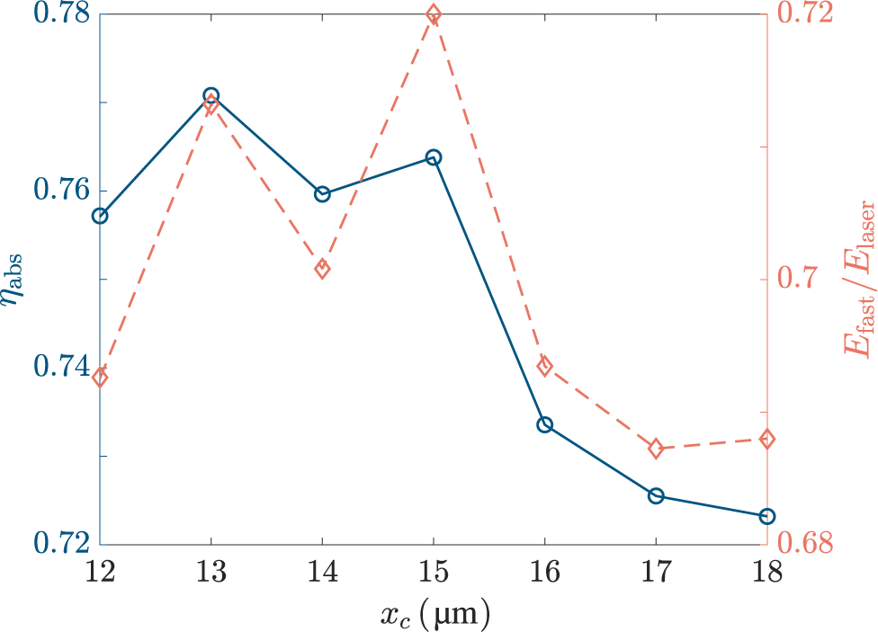
To determine the optimal crossing point more precisely under the large-angle configuration, we perform a detailed scan of
${x}_\mathrm{c}$
 at the fixed crossing angle
$\theta =60{}^{\circ}$
 and evaluate the corresponding laser absorption rate and fast-electron total energy collected at
$x=20\;\mu \mathrm{m}$
 , as shown in Figure 6. The crossing point is varied from
${x}_\mathrm{c}=12\;\mu \mathrm{m}$
 to
${x}_\mathrm{c}=18\;\mu \mathrm{m}$
 , focusing on the vicinity of the optimal crossing point of
${x}_\mathrm{c}=15\;\mu \mathrm{m}$
 identified in Figure 4. Both
${\eta}_{\mathrm{abs}}$
 and
${E}_{\mathrm{fast}}$
 exhibit non-monotonic dependence on
${x}_\mathrm{c}$
 . Notably, the maximum value of
${E}_{\mathrm{fast}}$
 is
$72.0\%$
 of the incident laser energy, obtained at
${x}_\mathrm{c}=15\;\mu \mathrm{m}$
 . At this position,
${\eta}_{\mathrm{abs}}$
 is
$76.38\%$
 , which is slightly lower than its maximum value of
$77.08\%$
 occurring at
${x}_\mathrm{c}=13\;\mu \mathrm{m}$
 . Since the fast-electron energy is the most relevant quantity for the subsequent heating process, we identify
${x}_\mathrm{c}=15\;\mu \mathrm{m}$
 as the optimal crossing point. This value is adopted as the reference crossing point in the simulations discussed in Section 4.
Laser absorption rate
$\left({\eta}_{\mathrm{abs}}\right)$
 and total energy of fast electrons
$\left({E}_{\mathrm{fast}}\right)$
 versus the crossing point of the laser pulses, where
${\eta}_{\mathrm{abs}}$
 and
${E}_{\mathrm{fast}}$
 are indicated by the blue solid and orange dashed curves, respectively. The crossing angle is fixed at
$\theta =60{}^{\circ}$
 .

Figure 6 Long description
The horizontal x-axis represents the crossing point x sub c in micrometers, ranging from 12 to 18. The left y-axis represents eta sub abs (laser absorption rate) with values from 0.72 to 0.78. The right y-axis represents E sub fast all over E sub laser (total energy of fast electrons) with values from 0.68 to 0.72.
* The blue solid line with circular markers (eta sub abs) starts at approximately 0.757 at x sub c equals 12, peaks at 0.771 at x sub c equals 13, fluctuates slightly through 15, and then drops sharply to a minimum of 0.723 at x sub c equals 18.
* The orange dashed line with diamond markers (E sub fast all over E sub laser) starts at 0.69 at x sub c equals 12, rises to 0.715 at x sub c equals 13, dips at 14, reaches its maximum peak of 0.72 at x sub c equals 15, and then declines to approximately 0.685 by x sub c equals 18.
Both curves show a general downward trend after x sub c equals 15.
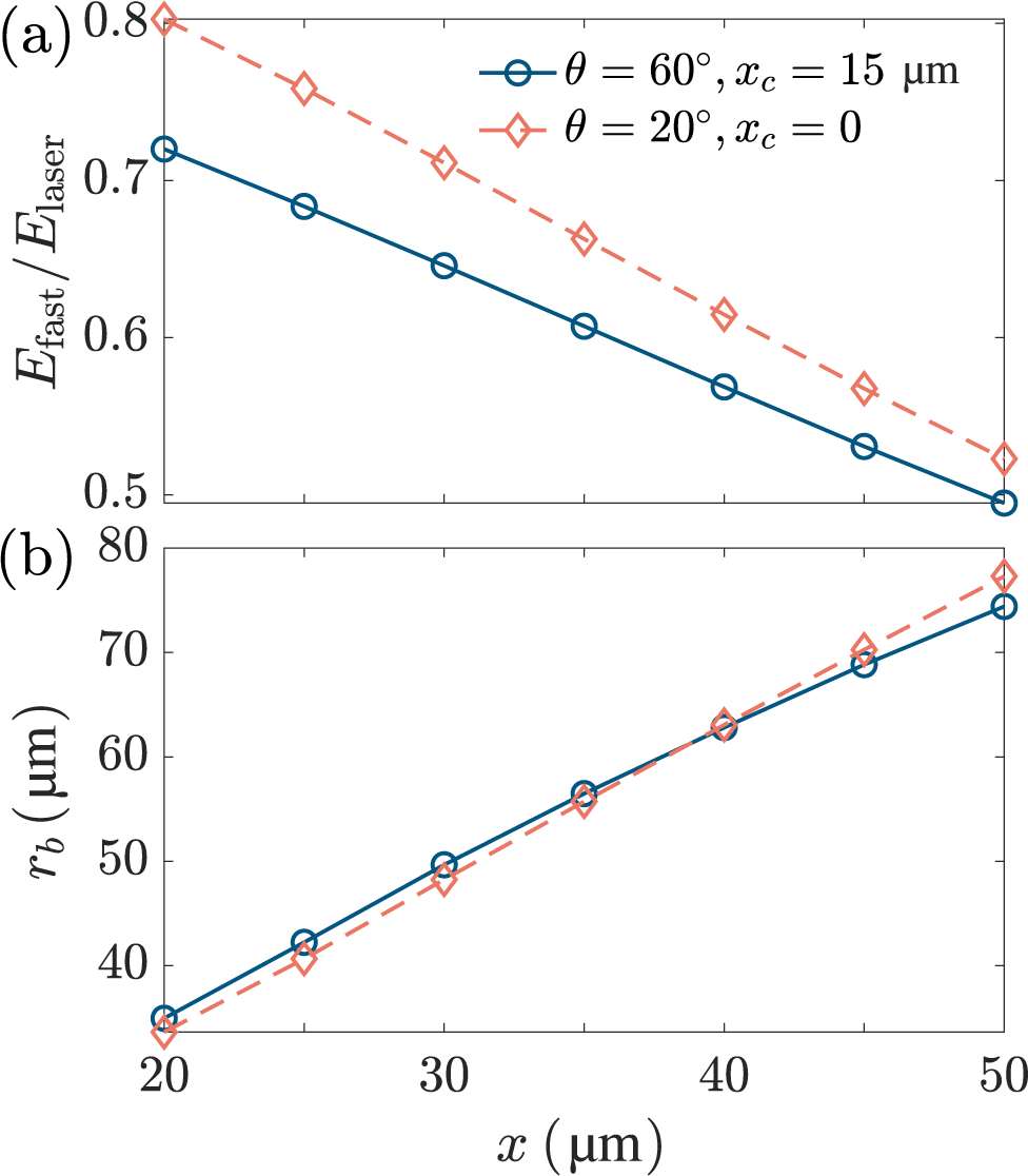
Figure 7(a) displays the total energy of fast electrons passing through each observing section from
$x=20\;\mu \mathrm{m}$
 to
$x=50\;\mu \mathrm{m}$
 . Two representative cases are compared: the optimized large-angle configuration with
$\theta =60{}^{\circ}$
 and
${x}_\mathrm{c}=15\;\mu \mathrm{m}$
 , and the optimal-angle configuration with
$\theta =20{}^{\circ}$
 and
${x}_\mathrm{c}=0$
 . As the fast electrons transport in the plasma target,
${E}_{\mathrm{fast}}$
 gradually decreases due to the energy depletion. At each observing section,
${E}_{\mathrm{fast}}$
 is lower for the
$\theta =60{}^{\circ}$
 and
${x}_\mathrm{c}=15\;\mu \mathrm{m}$
 case than for the
$\theta =20{}^{\circ}$
 and
${x}_\mathrm{c}=0$
 case. This indicates that although optimizing the crossing point substantially enhances fast-electron generation at a large crossing angle, the overall energy conversion efficiency of fast electrons remains lower than that achieved under the optimal-angle configuration without further optimization. Nevertheless, a clear difference is observed in the depletion rate of
${E}_{\mathrm{fast}}$
 during transport. The relative reduction of
${E}_{\mathrm{fast}}$
 from
$x=20\;\mu \mathrm{m}$
 to
$x=50\;\mu \mathrm{m}$
 is
$31.29\%$
 for the
$\theta =60{}^{\circ}$
 and
${x}_\mathrm{c}=15\;\mu \mathrm{m}$
 case, compared with
$34.86\%$
 for the
$\theta =20{}^{\circ}$
 and
${x}_\mathrm{c}=0$
 case, indicating more efficient energy transport in the optimized large-angle configuration. The reduced energy depletion rate can be attributed to the difference in the effective transport distance and divergence of fast electrons. For the
$\theta =20{}^{\circ}$
 and
${x}_\mathrm{c}=0$
 case, a substantial fraction of fast electrons is generated below the critical density and must propagate over a relatively long distance before reaching the observing section at
$x=20\;\mu \mathrm{m}$
 . During this transport, the fast-electron beam undergoes significant transverse divergence, resulting in severe energy loss. In contrast, when
${x}_\mathrm{c}=15\;\mu \mathrm{m}$
 at
$\theta =60{}^{\circ}$
 , fast electrons are predominantly generated within a few
${n}_\mathrm{c}$
 , closer to the observing section at
$x=20\;\mu \mathrm{m}$
 , leaving less distance for divergence to develop. This interpretation is further supported by the evolution of the transverse size of the fast-electron beam, as shown in Figure 7(b). Here
${r}_\mathrm{b}$
 represents the full width at half maximum (FWHM) of the transverse size of the fast-electron beam, fitted by a Gaussian function. Although
${r}_\mathrm{b}$
 is initially larger at
$x=20\;\mu \mathrm{m}$
 for the
$\theta =60{}^{\circ}$
 and
${x}_\mathrm{c}=15\;\mu \mathrm{m}$
 case, its growth with transport distance is slower, resulting in a smaller beam size at
$x=50\;\mu \mathrm{m}$
 . This slower expansion indicates reduced transverse divergence during transport, which is consistent with the lower energy depletion rate observed in Figure 7(a) and is favorable for subsequent fuel heating.
(a) Total energy and (b) transverse FWHM size of the fast-electron beam passing through the observing sections from
$x=20\;\mu \mathrm{m}$
 to
$x=50\;\mu \mathrm{m}$
 . In each plot, the blue solid curve and orange dashed curve correspond to the cases of
$\theta =60{}^{\circ},\ {x}_\mathrm{c}=15\;\mu \mathrm{m}$
 and
$\theta =20{}^{\circ},\ {x}_\mathrm{c}=0$
 , respectively.

Figure 7 Long description
The figure consists of two vertically stacked line graphs sharing a common x-axis labeled x in mu m, ranging from 20 to 50.
Panel a: The y-axis is labeled E sub fast all over E sub laser, ranging from 0.5 to 0.8. Two data series are shown. The first, represented by a blue solid line with open circles, corresponds to theta equals 60 degrees and x sub c equals 15 mu m. It shows a linear decrease from approximately 0.72 at x equals 20 to 0.5 at x equals 50. The second, represented by an orange dashed line with open diamonds, corresponds to theta equals 20 degrees and x sub c equals 0. It shows a steeper linear decrease from 0.8 at x equals 20 to approximately 0.52 at x equals 50.
Panel b: The y-axis is labeled r sub b in mu m, ranging from 30 to 80. Both data series show a linear increase. The blue solid line with circles starts at approximately 35 at x equals 20 and rises to 75 at x equals 50. The orange dashed line with diamonds starts slightly lower at 34 at x equals 20 and rises to a higher final value of 78 at x equals 50, crossing the blue line at approximately x equals 40.
It should be noted that the motion of a single electron in obliquely crossing relativistic laser pulses could be highly nonlinear and may appear chaotically sensitive to numerical methods and initial conditions, as discussed by Robinson et al.
[
Reference Robinson, Tangtartharakul, Weichman and Arefiev
53
]. To address this concern, we perform additional numerical robustness tests for three typical cases:
$\left(\theta =20{}^{\circ},{x}_\mathrm{c}=0\right)$
 ,
$\left(\theta =60{}^{\circ},{x}_\mathrm{c}=0\right)$
 and
$\left(\theta =60{}^{\circ},{x}_\mathrm{c}=15\;\mu \mathrm{m}\right)$
 in our work. These cases correspond to the optimal-angle configuration, the large-angle configuration without crossing-point optimization and the optimized large-angle configuration discussed in Sections 2 and 3. In the three cases, we carry out additional simulations with a higher resolution of
$\Delta x=\Delta y={\lambda}_\mathrm{L}/48$
 than the baseline resolution of
$\Delta x=\Delta y={\lambda}_\mathrm{L}/32$
 . The comparison between the two resolutions shows that the simulations are numerically convergent, as illustrated in Figures 10 and 11 in Appendix A.
4 Magnetic-field guiding of fast-electron transport in the optimized geometry
As shown in Figure 7, fast electrons undergo significant energy depletion during transport in plasma, primarily due to their transverse divergence. Reducing this energy depletion is essential for maintaining the fast-electron energy available for the subsequent fuel heating in FI. One effective approach to confine fast-electron divergence is the application of an external strong magnetic field of approximately kT. Here, we investigate the impact of an externally applied uniform magnetic field on fast-electron generation and transport. The laser configuration is fixed at the optimized condition obtained in Section 3, with a crossing angle of
$\theta =60{}^{\circ}$
 and a crossing point of
${x}_\mathrm{c}=15\;\mu \mathrm{m}$
 . The magnetic field is assumed to be spatially uniform along the
$+x$
 direction, and the field strengths are taken as
$B=0$
 ,
$0.5\;\mathrm{kT}$
 ,
$1\;\mathrm{kT}$
 ,
$1.5\;\mathrm{kT}$
 and
$2\;\mathrm{kT}$
 . This configuration approximates the quasi-uniform magnetic field generated by a coil target with diameter larger than
$500\;\mu \mathrm{m}$
 , which has been demonstrated in previous studies[
Reference Wang, Zhang and Wang
39
] and is commonly used in experiments to generate
$\mathrm{kT}$
 -level magnetic fields[
Reference Bailly-Grandvaux, Santos, Bellei, Forestier-Colleoni, Fujioka, Giuffrida, Honrubia, Batani, Bouillaud, Chevrot, Cross, Crowston, Dorard, Dubois, Ehret, Gregori, Hulin, Kojima, Loyez, Marques, Morace, Nicolai, Roth, Sakata, Schaumann, Serres, Servel, Tikhonchuk, Woolsey and Zhang
40
,
Reference Sakata, Lee, Morita, Johzaki, Sawada, Iwasa, Matsuo, Law, Yao, Hata, Sunahara, Kojima, Abe, Kishimoto, Syuhada, Shiroto, Morace, Yogo, Iwata, Nakai, Sakagami, Ozaki, Yamanoi, Norimatsu, Nakata, Tokita, Miyanaga, Kawanaka, Shiraga, Mima, Nishimura, Bailly-Grandvaux, Santos, Nagatomo, Azechi, Kodama, Arikawa, Sentoku and Fujioka
41
,
Reference Law, Bailly-Grandvaux, Morace, Sakata, Matsuo, Kojima, Lee, Vaisseau, Arikawa, Yogo, Kondo, Zhang, Bellei, Santos, Fujioka and Azechi
54
,
Reference Zhang, Zhu, Li, Jiang, Yuan, Wei, Liang, Wang, Zhao, Zhong, Han, Hua, Zhu, Zhu, Wang, Fang and Zhang
55
]. Under these conditions, the applied magnetic field primarily acts to reduce the transverse divergence of fast electrons and improve transport efficiency.
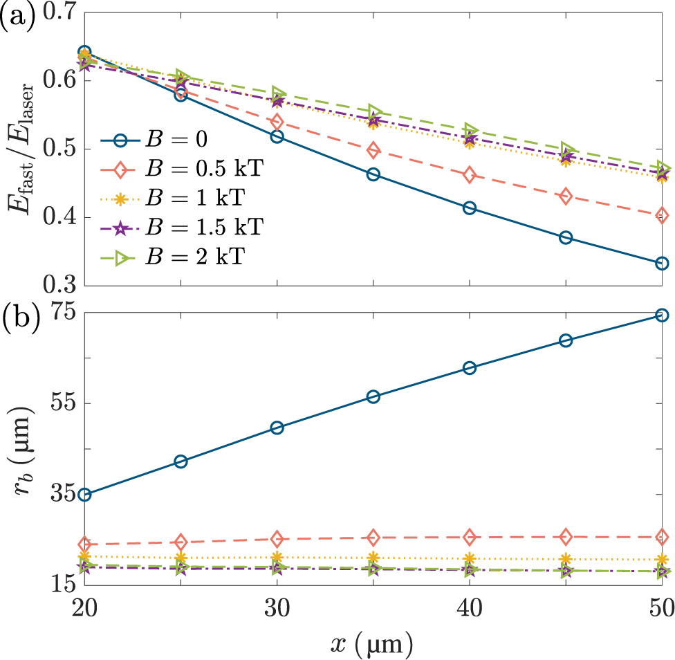
Figure 8 shows the total energy within
$-24\;\mu \mathrm{m}<y<24\;\mu \mathrm{m}$
 and transverse size of the fast-electron beams at each observing section for various externally applied magnetic-field strengths. At the generation region, for example,
$x=20\;\mu \mathrm{m}$
 ,
${E}_{\mathrm{fast}}$
 slightly decreases as
$B$
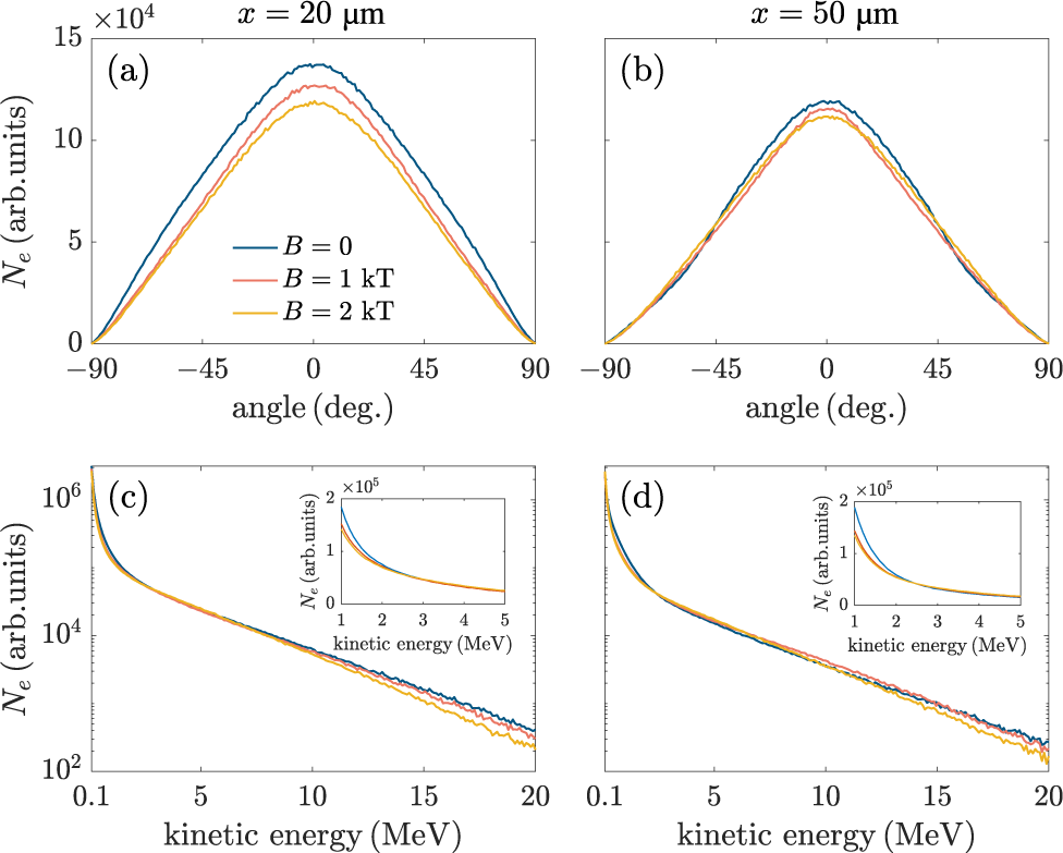
 increases, indicating that the external magnetic field does not enhance fast-electron generation. This behavior is further illustrated by the angle spectra and energy spectra shown in Figure 9. As shown in Figure 9(a), the total number of fast electrons decreases with increasing magnetic-field strength at
$x=20\;\mu \mathrm{m}$
 . The corresponding energy spectra in Figure 9(c) exhibit a similar trend, with fewer fast electrons collected across the energy range from
$0.1$
 to
$20\;\mathrm{MeV}$
 when a magnetic field is applied. We attribute this reduction to the modification of electron dynamics in the laser field by the externally applied magnetic field. The presence of a
$\mathrm{kT}$
 -level magnetic field suppresses transverse electron oscillations associated with
$\mathbf{J}\times \mathbf{B}$
 heating, thereby reducing the number of electrons that can be efficiently accelerated.
(a) Total energy within
$-24\;\mu \mathrm{m}<y<24\;\mu \mathrm{m}$
 and (b) transverse FWHM size of the fast-electron beam passing through the observing sections from
$x=20\;\mu \mathrm{m}$
 to
$x=50\;\mu \mathrm{m}$
 . In each plot, five curves correspond to the magnetic-field strengths of
$B=0$
 (blue solid curve),
$B=0.5\;\mathrm{kT}$
 (orange dashed curve),
$B=1\;\mathrm{kT}$
 (yellow dot curve),
$B=1.5\;\mathrm{kT}$
 (purple dashed dot curve) and
$B=2\;\mathrm{kT}$
 (green dashed dot curve), respectively.

Figure 8 Long description
Two vertically stacked line graphs share a horizontal x-axis labeled x in mu m, ranging from 20 to 50.
Panel a, the top graph, has a vertical y-axis labeled E sub fast over E sub laser, ranging from 0.3 to 0.7. It shows five downward-sloping curves. The blue solid line with circles (B = 0) shows the steepest linear decline from 0.65 to 0.33. As the magnetic field increases to 0.5 k T (orange dashed with diamonds), 1 k T (yellow dotted with stars), 1.5 k T (purple dash-dot with stars), and 2 k T (green dash-dot with triangles), the curves become progressively flatter and maintain higher energy ratios, with the 2 k T curve ending at approximately 0.48.
Panel b, the bottom graph, has a vertical y-axis labeled r sub b in mu m, ranging from 15 to 75. The blue solid line (B = 0) shows a sharp linear increase from 35 to 75. In contrast, the four curves representing magnetic fields from 0.5 k T to 2 k T are nearly horizontal and clustered at the bottom of the plot. The 0.5 k T curve stays near 25 mu m, while the 1, 1.5, and 2 k T curves are tightly grouped between 18 and 20 mu m, indicating suppressed beam expansion.
Angle spectra (top row) and energy spectra (bottom row) of fast electrons passing through the
$x=20\;\mu \mathrm{m}$
 section (left-hand column) and
$x=50\;\mu \mathrm{m}$
 section (right-hand column). In each plot, three curves correspond to the magnetic-field strength with
$B=0$
 (blue curve),
$B=1\;\mathrm{kT}$
 (orange curve) and
$B=2\;\mathrm{kT}$
 (yellow curve), respectively.

Figure 9 Long description
A four-panel figure showing angle spectra (top row) and energy spectra (bottom row) of fast electrons at x = 20 micrometers (left-hand column) and x = 50 micrometers (right-hand column).
Top row, angle spectra.
Panel a, x equals 20 mu m. The y-axis is N sub e in arbitrary units times 10 super 4, ranging from 0 to 15. The x-axis is angle in degrees from negative 90 to 90. Three bell-shaped curves peak at 0 degrees. The blue curve B equals 0 has the highest peak at approximately 14. The orange curve B equals 1 k T is slightly lower. The yellow curve B equals 2 k T has the lowest peak at approximately 12.
Panel b, x equals 50 mu m. Similar bell curves but with lower overall intensity, peaking at approximately 12 for B equals 0 and 11 for B equals 2 k T.
Bottom row, energy spectra.
Panel c, x equals 20 mu m. The y-axis is N sub e in arbitrary units on a logarithmic scale from 10 super 2 to 10 super 6. The x-axis is kinetic energy in M e V from 0.1 to 20. All three curves show a steep exponential decay. An inset graph shows the low-energy region from 1 to 5 M e V on a linear scale. The blue curve remains highest, followed by orange and yellow.
Panel d, x equals 50 mu m. Similar exponential decay to panel c, but the separation between the curves at high kinetic energy is more pronounced, with the yellow curve B equals 2 k T showing the lowest electron count.
Although the external magnetic field slightly reduces fast-electron generation, it significantly enhances fast-electron transport. As shown in Figure 8(a), at each observing section from
$x=25\;\mu \mathrm{m}$
 to
$x=50\;\mu \mathrm{m}$
 ,
${E}_{\mathrm{fast}}$
 gradually increases as the magnetic-field strength is increased from
$B=0$
 to
$B=2\;\mathrm{kT}$
 , indicating reduced energy loss during transport. The corresponding beam size
${r}_\mathrm{b}$
 in Figure 8(b) decreases significantly when an external magnetic field is applied. In the absence of a magnetic field, that is,
$B=0$
 ,
${r}_\mathrm{b}$
 increases rapidly as fast electrons transport from
$x=20\;\mu \mathrm{m}$
 to
$x=50\;\mu \mathrm{m}$
 , reflecting strong transverse divergence during transport. When the magnetic field is increased to
$B=0.5\;\mathrm{kT}$
 ,
${r}_\mathrm{b}$
 becomes nearly independent of the transport distance
$x$
 . Further increasing the magnetic field to 1, 1.5 and
$2\;\mathrm{kT}$
 produces only minor additional changes in
${r}_\mathrm{b}$
 , indicating that the confinement effect approaches saturation as the magnetic-field strength is above
$0.5\;\mathrm{kT}$
 .
The saturation around
$B\sim 0.5\;\mathrm{kT}$
 should be interpreted as the quasi-saturated suppression of the transverse widening of the fast-electron beam under the present simulation parameters, rather than as a universal saturation field. This behavior can be qualitatively understood from the Larmor-radius scaling:

where
${p}_{\perp }={\left({p}_y^2+{p}_z^2\right)}^{1/2}$
 is the transverse momentum of fast electrons. For
$B=0.5\;\mathrm{kT}$
 , one obtains
${r}_\mathrm{L}\simeq 3.4\left({p}_{\perp }/{m}_\mathrm{e}c\right)\;[\mu \mathrm{m}]$
 . Thus, for transverse momenta of the order of a few
${m}_\mathrm{e}c$
 , which are relevant for
$\mathrm{MeV}$
 -level fast electrons, the Larmor radius is of the order of several to ten micrometers, comparable to the transverse scale of the guided fast-electron beam in Figure 8(b). Once this condition is reached, the beam widening is efficiently suppressed, and further increasing
$B$
 produces only minor additional reduction in
${r}_\mathrm{b}$
 . However, the magnetic-field scale at which
${E}_{\mathrm{fast}}$
 approaches a plateau can depend on laser and plasma parameters, as further examined in Appendix B.
As fast electrons transport to
$x=50\;\mu \mathrm{m}$
 , the differences between the angle spectra and energy spectra become smaller, as shown in Figures 9(b) and 9(d). The peak values of the angle spectra becomes nearly identical, indicating that magnetic-field guiding effectively suppresses transverse expansion of fast electrons during transport. Consequently, although fewer fast electrons are initially generated in the presence of a strong magnetic field, their transverse widening is significantly reduced, allowing more electrons to remain confined within the plasma region. It is worth noting that the overall shapes of the angle spectra and energy spectra present little variation between
$x=20\;\mu \mathrm{m}$
 and
$x=50\;\mu \mathrm{m}$
 , indicating that the uniform magnetic field primarily influences fast-electron transport rather than their intrinsic angular and energy distributions. Since magnetic fields of the order of
$0.5\;\mathrm{kT}$
 have already been achieved in magnetically guided FI experiments[
Reference Bailly-Grandvaux, Santos, Bellei, Forestier-Colleoni, Fujioka, Giuffrida, Honrubia, Batani, Bouillaud, Chevrot, Cross, Crowston, Dorard, Dubois, Ehret, Gregori, Hulin, Kojima, Loyez, Marques, Morace, Nicolai, Roth, Sakata, Schaumann, Serres, Servel, Tikhonchuk, Woolsey and Zhang
40
,
Reference Sakata, Lee, Morita, Johzaki, Sawada, Iwasa, Matsuo, Law, Yao, Hata, Sunahara, Kojima, Abe, Kishimoto, Syuhada, Shiroto, Morace, Yogo, Iwata, Nakai, Sakagami, Ozaki, Yamanoi, Norimatsu, Nakata, Tokita, Miyanaga, Kawanaka, Shiraga, Mima, Nishimura, Bailly-Grandvaux, Santos, Nagatomo, Azechi, Kodama, Arikawa, Sentoku and Fujioka
41
], a uniform magnetic field of approximately
$0.5\;\mathrm{kT}$
 provides an effective and experimentally achievable choice for guiding fast-electron transport in the present large-angle configuration.
5 Summary
In summary, we have investigated the impact of the spatial configuration of two picosecond laser pulses on fast-electron generation and transport by PIC simulations. A large crossing angle of
$\theta =60{}^{\circ}$
 is found to reduce laser absorption and fast-electron generation compared with the optimized angle around
$\theta =20{}^{\circ}$
 , mainly due to degraded laser–plasma coupling and disrupted surface structures. To mitigate these unfavorable factors, we propose an approach shifting the laser pulse crossing point
${x}_\mathrm{c}$
 from the vacuum–plasma boundary into the plasma interior. Our simulation results show that the total energy of fast electrons is maximized when the crossing point is located near the laser hole boring depth, that is,
${x}_\mathrm{c}=15\;\mu \mathrm{m}$
 , where the two laser pulses overlap near the critical-density region and a more stable plasma surface structure enhances the
$\mathbf{J}\times \mathbf{B}$
 heating. An external uniform magnetic field is also introduced to guide fast-electron transport under this configuration. The simulations suggest that sub-
$\mathrm{kT}$
 magnetic fields effectively suppress the energy depletion and divergent motion of fast electrons. Under the present simulation parameters, the suppression of beam divergence becomes nearly saturated at
$B\sim 0.5\;\mathrm{kT}$
 . This work could be applied in DCI and FI schemes of laser fusion and applications based on MeV-level electron generation by multiple ps laser pulses, such as ion acceleration and radiation sources.
Appendix A Numerical robustness tests for PIC simulations of crossed laser pulses
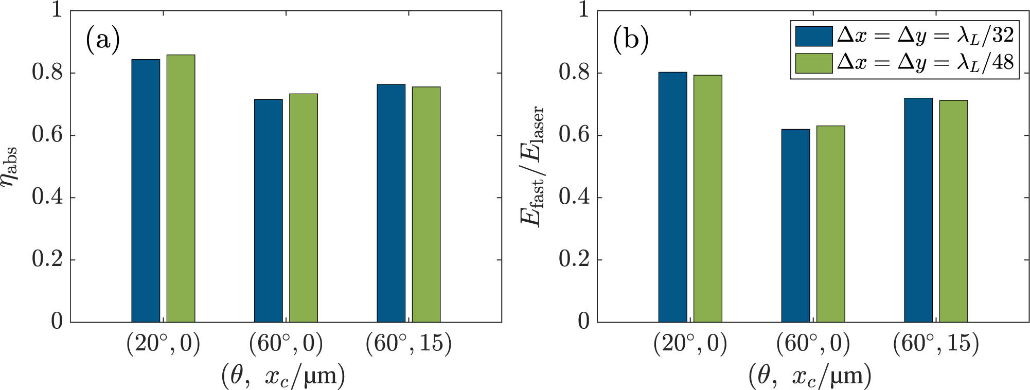
Figures 10(a) and 10(b) present the laser absorption rate
${\eta}_{\mathrm{abs}}$
 and the total energy of forward fast electrons
${E}_{\mathrm{fast}}$
 collected at
$x=20\;\mu \mathrm{m}$
 , respectively. For all three cases, both
${\eta}_{\mathrm{abs}}$
 and
${E}_{\mathrm{fast}}$
 remain essentially unchanged for the different resolutions. In particular, the reduction of fast-electron generation at
$\theta =60{}^{\circ}$
 and the enhancement obtained by shifting the crossing point to
${x}_\mathrm{c}=15\;\mu \mathrm{m}$
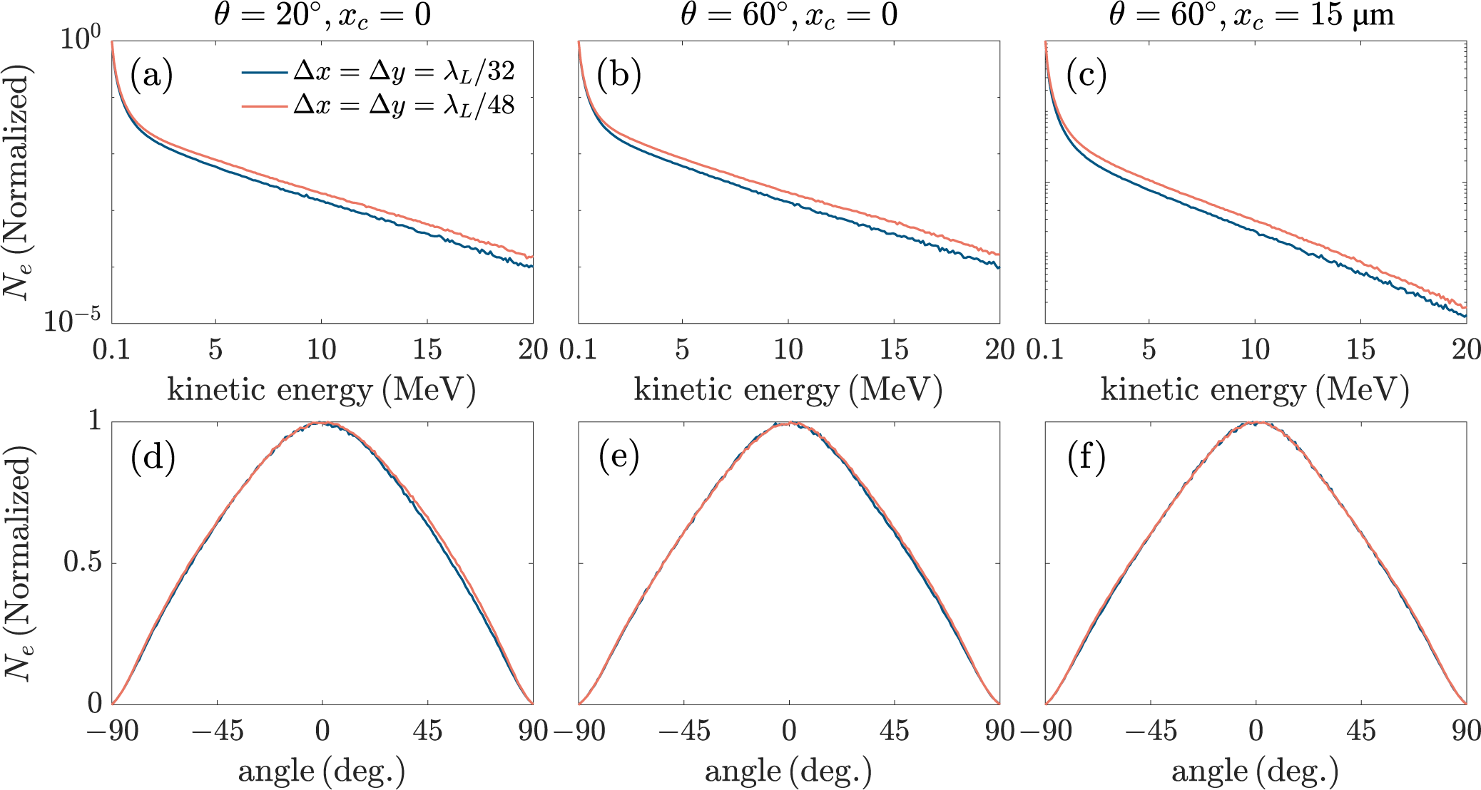
 are both preserved. We further compare the normalized energy spectra and angle spectra of fast electrons in Figure 11. The energy spectra for the two resolutions show similar slopes and overall distributions. Small differences appear only in the high-energy tail, where the particle number is relatively low. The angle spectra almost overlap in all three cases with different resolutions, indicating that the fast-electron divergence is numerically convergent.
(a) Laser absorption rate and (b) total energy of fast electrons passing through the
$x=20\;\mu \mathrm{m}$
 section versus three cases of
$\left(\theta =20{}^{\circ},{x}_\mathrm{c}=0\right)$
 ,
$\left(\theta =60{}^{\circ},{x}_\mathrm{c}=0\right)$
 and
$\left(\theta =60{}^{\circ},{x}_\mathrm{c}=15\;\mu \mathrm{m}\right)$
 . In each plot, the blue bar and green bar represent spatial resolutions of
$\Delta x=\Delta y={\lambda}_\mathrm{L}/32$
 and
$\Delta x=\Delta y={\lambda}_\mathrm{L}/48$
 , respectively.

Figure 10 Long description
A two-panel figure labeled a and b. Both panels share a common horizontal axis representing three cases of theta and x sub c in micrometers: 20 degrees, 0; 60 degrees, 0; and 60 degrees, 15. Each case contains a blue bar for delta x equals delta y equals lambda sub L over 32 and a green bar for delta x equals delta y equals lambda sub L over 48.
* Panel a: The vertical axis is eta sub abs, ranging from 0 to 1. For the 20 degrees, 0 case, absorption is approximately 0.85. For 60 degrees, 0, it drops to approximately 0.72. For 60 degrees, 15, it is approximately 0.76. The green bars show slightly higher absorption than blue bars in the first two cases.
* Panel b: The vertical axis is E sub fast over E sub laser, ranging from 0 to 1. The energy ratio is highest for the 20 degrees, 0 case at approximately 0.8, lowest for the 60 degrees, 0 case at approximately 0.62, and intermediate for the 60 degrees, 15 case at approximately 0.72. The blue and green bars show very similar values across all three configurations.
Normalized energy spectra (top row) and angle spectra (bottom row) of fast electrons passing through the
$x=20\;\mu \mathrm{m}$
 section. The first to third columns correspond to the cases of
$\left(\theta =20{}^{\circ},{x}_\mathrm{c}=0\right)$
 ,
$\left(\theta =60{}^{\circ},{x}_\mathrm{c}=0\right)$
 and
$\left(\theta =60{}^{\circ},{x}_\mathrm{c}=15\;\mu \mathrm{m}\right)$
 , respectively. In each plot, the blue curve and orange curve represent spatial resolutions of
$\Delta x=\Delta y={\lambda}_\mathrm{L}/32$
 and
$\Delta x=\Delta y={\lambda}_\mathrm{L}/48$
 , respectively.

Figure 11 Long description
The figure consists of six panels labeled a through f.
Top Row (Energy Spectra):
Panels a, b, and c show normalized N sub e on a logarithmic Y-axis (from 10 super minus 5 to 10 super 0) versus kinetic energy in M e V on a linear X-axis (from 0.1 to 20).
* Panel a (theta = 20 degrees, x sub c = 0): Both curves show a steep initial drop followed by a gradual exponential decay. The orange curve (delta x = delta y = lambda sub L all over 48) remains slightly higher than the blue curve (delta x = delta y = lambda sub L all over 32) as energy increases.
* Panel b (theta = 60 degrees, x sub c = 0): Similar decay trend, but the divergence between the orange and blue curves is more pronounced than in panel a.
* Panel c (theta = 60 degrees, x sub c = 15 mu m): The curves show the lowest overall intensity at high energies compared to panels a and b, with the orange curve maintaining a higher normalized count than the blue.
Bottom Row (Angle Spectra):
Panels d, e, and f show normalized N sub e on a linear Y-axis (from 0 to 1) versus angle in degrees on a linear X-axis (from minus 90 to 90).
* All three panels (d, e, and f) display a symmetric Gaussian-like bell curve centered at 0 degrees.
* In all cases, the blue and orange curves are nearly perfectly overlapped, indicating that spatial resolution has a negligible effect on the angular distribution of the electrons.
These results demonstrate that the statistical quantities used in this work, including
${\eta}_{\mathrm{abs}}$
 ,
${E}_{\mathrm{fast}}$
 , the energy spectra and the angle spectra, are numerically robust against the resolutions of
${\lambda}_\mathrm{L}/32$
 and
${\lambda}_\mathrm{L}/48$
 . Although individual electron trajectories in crossed laser fields may be sensitive to numerical parameters, the agreement between the cases with
${\lambda}_\mathrm{L}/32$
 and
${\lambda}_\mathrm{L}/48$
 in Figures 10 and 11 indicates that the key statistical quantities of interest are not significantly affected.
Appendix B Parameter dependence of magnetic-field guiding
To further examine the parameter dependence of the magnetic-field guiding discussed in Section 4, we perform an additional set of simulations with a higher laser intensity of
${10}^{20}\;\mathrm{W}/{\mathrm{cm}}^2$
 and a lower plasma density of
$50{n}_\mathrm{c}$
 . The external magnetic field is assumed to be spatially uniform along the
$+x$
 direction, and its strength is scanned over
$B=0$
 ,
$0.5\;\mathrm{kT}$
 ,
$1\;\mathrm{kT}$
 ,
$1.5\;\mathrm{kT}$
 and
$2\;\mathrm{kT}$
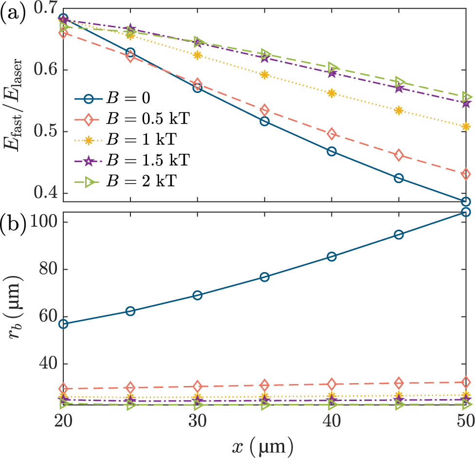
 . Similar to Figure 8, we present the total energy within
$-24\;\mu \mathrm{m}<y<24\;\mu \mathrm{m}$
 and the transverse size of the fast-electron beams at each observing section in Figure 12.
(a) Total energy within
$-24\;\mu \mathrm{m}<y<24\;\mu \mathrm{m}$
 and (b) transverse FWHM size of the fast-electron beam passing through the observing sections from
$x=20\;\mu \mathrm{m}$
 to
$x=50\;\mu \mathrm{m}$
 , where a laser intensity of
${10}^{20}\;\mathrm{W}/{\mathrm{cm}}^2$
 and a plasma density of
$50{n}_\mathrm{c}$
 are adopted. In each plot, five curves correspond to the magnetic-field strengths of
$B=0$
 (blue solid curve),
$B=0.5\;\mathrm{kT}$
 (orange dashed curve),
$B=1\;\mathrm{kT}$
 (yellow dot curve),
$B=1.5\;\mathrm{kT}$
 (purple dashed dot curve) and
$B=2\;\mathrm{kT}$
 (green dashed dot curve), respectively.

Figure 12 Long description
Panel a displays the energy ratio E sub fast all over E sub laser on the y-axis, ranging from 0.4 to 0.7, against distance x in micrometers on the x-axis, ranging from 20 to 50. All five curves show a downward trend. The blue solid curve for B equals 0 has the steepest decline, dropping from approximately 0.68 to 0.39. As the magnetic field B increases to 0.5 k T (orange dashed), 1 k T (yellow dotted), 1.5 k T (purple dash-dot), and 2 k T (green dash-dot), the curves become progressively flatter and maintain higher energy ratios at x equals 50.
Panel b displays the transverse F W H M size r sub b in micrometers on the y-axis, ranging from 20 to 100, against the same x-axis. The blue solid curve for B equals 0 shows a significant linear increase from approximately 58 to over 100 micrometers. In contrast, the four curves representing magnetic fields from 0.5 k T to 2 k T remain nearly horizontal and tightly clustered at the bottom of the graph, with r sub b values staying below 35 micrometers throughout the distance range.
As shown in Figure 12(b),
${r}_\mathrm{b}$
 still becomes nearly flat when
$B$
 is increased to about
$0.5\;\mathrm{kT}$
 , indicating that the suppression of beam widening enters a quasi-saturated regime. However, the transported fast-electron energy
${E}_{\mathrm{fast}}$
 shows a clearer parameter dependence. In the baseline case shown in Figure 8(a), the curves for
$B=1\;\mathrm{kT}$
 ,
$1.5\;\mathrm{kT}$
 and
$2\;\mathrm{kT}$
 are close to each other. By contrast, in Figure 12(a), the
$B=1\;\mathrm{kT}$
 curve remains visibly separated from the
$B=1.5\;\mathrm{kT}$
 and
$2\;\mathrm{kT}$
 curves, while the latter two are close to each other. This comparison indicates that the field scale at which
${E}_{\mathrm{fast}}$
 approaches a plateau shifts to a higher value under the higher laser intensity and lower plasma density conditions.
These results suggest that
$B\sim 0.5\;\mathrm{kT}$
 should not be regarded as a universal saturation amplitude. Rather, it is the characteristic field scale for the onset of quasi-saturated suppression of fast-electron beam transverse widening under the simulation parameters of Sections 2–4. The magnetic-field strength required for
${E}_{\mathrm{fast}}$
 to become nearly insensitive to further increases in
$B$
 can vary with the laser intensity, plasma density and other laser–plasma parameters.
Acknowledgements
This work was supported by the Shanghai Municipal Science and Technology Major Project, the Strategic Priority Research Program of Chinese Academy of Sciences (Grant No. XDA25050300) and the Fundamental Research Funds for the Central Universities, the Research Funds of Shanghai Jiao Tong University (WH220207203).
























 Open access

