INTRODUCTION
It has been suggested that the Holocene sea level was modulated by a combination of factors that perturbed the land-sea configuration (Lambeck et al., Reference Lambeck, Rouby, Purcell, Sun and Sambridge2014; Vacchi et al., Reference Vacchi, Rovere, Chatzipetros, Zouros and Firpo2014; Engelhart et al., Reference Engelhart, Vacchi, Horton, Nelson and Kopp2015). These include tectonic instability, coastal configuration changes, proximity of the sites to meltwater discharge, sediment flux, and most importantly the post–last glacial maximum (LGM) glacio-isostatic adjustment (GIA) in the higher latitudes (Newman et al., Reference Newman, Pardi, Fairbridge, Scott, Pirazzoli and Honig1989; Shennan and Horton, Reference Shennan and Horton2002; Ferrier et al., Reference Ferrier, Mitrovica, Giosan and Clift2015). Therefore, a generalized global time/depth Holocene sea-level curve would be misleading (Pirazzoli, Reference Pirazzoli1991). To ascertain the eustatic component (glacial melt and hence the climate) for Holocene relative sea-level (RSL) change, it is suggested that the focus should be on tectonically stable and far-field locations from the LGM ice margins (Clark et al., Reference Clark, Farrell and Peltier1978).
In the far-field locations (away from ice sheets), the GIA depends significantly on equatorial ocean siphoning and hydro-isostasy (continental levering) (Clark et al., Reference Clark, Farrell and Peltier1978; Newman et al., Reference Newman, Pardi, Fairbridge, Scott, Pirazzoli and Honig1989; Mitrovica and Milne, Reference Mitrovica and Milne2002; Shennan and Horton, Reference Shennan and Horton2002; Ferrier et al., Reference Ferrier, Mitrovica, Giosan and Clift2015). Equatorial ocean siphoning redistributes ocean water from the equator to higher latitudes because of subsiding peripheral fore-bulges and sub-lithospheric mantle flow (Mitrovica and Peltier, Reference Mitrovica and Peltier1991; Peltier, Reference Peltier1999). Continental levering refers to hydro-isostatic subsidence of the oceanic crust and uplift of coastlines (Mitrovica and Milne, Reference Mitrovica and Milne2002; Mann et al., Reference Mann, Bender, Lorscheid, Stocchi, Vacchi, Switzer and Rovere2019). Researchers have argued that these processes were important, particularly for the Late Holocene RSL fall in the low latitudes (Mitrovica and Milne, Reference Mitrovica and Milne2002), including the Indian Ocean (Woodroffe et al., Reference Woodroffe, McLean, Polach and Wallensky1990; Kench et al., Reference Kench, Smithers, Mclean and Nichol2009). Therefore, to ascertain the eustatic component, the non-eustatic components need to be accounted for (Mitrovica and Peltier, Reference Mitrovica and Peltier1991).
Along the Indian coast, limited studies suggest significant changes in the magnitude of the Holocene sea level (Banerjee, Reference Banerjee1993, Reference Banerjee2000; Pant and Juyal, Reference Pant and Juyal1993; Juyal et al., Reference Juyal, Pant, Bhushan and Somayajulu1995; Kunte and Wagle, Reference Kunte and Wagle2005; Bhatt and Bhonde, Reference Bhatt and Bhonde2006; Banerji et al., Reference Banerji, Pandey, Bhushan and Juyal2015) (Fig. 1A). Banerjee (Reference Banerjee2000) estimated Holocene sea level from the passive margin boundary (tectonically stable) on the eastern Indian coast. The study suggests an ~3 m high stand above low tide level at ~7 ka, and an ~1 m high stand between 5.2 and 4.2 ka. From the tectonically active western coast of India (Saurashtra peninsula), the chronology of the raised oyster beds indicates that Holocene sea level fluctuated between 2 and 3 m above mean sea level (amsl) from 8.6 to 2.5 ka (Pant and Juyal, Reference Pant and Juyal1993; Juyal et al., Reference Juyal, Pant, Bhushan and Somayajulu1995). More recently, Banerji et al. (Reference Banerji, Pandey, Bhushan and Juyal2015), after accounting for the tectonic component, suggested that the Mid-Holocene sea level in the Saurashtra Peninsula was ~1 m higher than the present. A similar observation was made by Brückner (Reference Brückner, Scott, Pirazoli and Honig1989), suggesting that between 6 and 5 ka, the sea level was ~1 m higher than the present along coastal Saurashtra. Compared to coastal Saurashtra, the Holocene sea-level studies from the tectonically active Kachchh coastline (Bhattacharya et al., Reference Bhattacharya, Rastogi, Thakkar, Patel and Juyal2014, Reference Bhattacharya, Chauhan, Prasad, Patel and Thakkar2019) are limited and also lack robust estimates from a common datum. Gupta (Reference Gupta1975) suggested ~4–m-deep water at ~2 ka in the Little Rann. According to Khonde et al. (Reference Khonde, Maurya, Singh, Chowksey and Chamyal2011), marine sedimentation continued in the Great Rann until 1500 AD. In contrast, Tyagi et al. (Reference Tyagi, Shukla, Bhushan, Thakker, Thakkar and Juyal2012) suggested that the western Great Rann was under the influence of tidal-flat sedimentation between 5.5 and 2 ka. Recently, Das et al. (Reference Das, Prizomwala, Makwana and Thakkar2017) estimated ~2–m-high sea level between 6 and 3 ka from the Gulf of Kachchh. These studies indicate that RSL fluctuated significantly and that, in addition to eustacy, hydro-isostasy (Banerjee, Reference Banerjee2000), tectonic upliftment (Pant and Juyal, Reference Pant and Juyal1993; Juyal et al., Reference Juyal, Pant, Bhushan and Somayajulu1995; Banerji et al., Reference Banerji, Pandey, Bhushan and Juyal2015), coastal configuration modifications, and sediment deposition by alongshore current near the Indus delta (Ferrier et al., Reference Ferrier, Mitrovica, Giosan and Clift2015) are considered important.
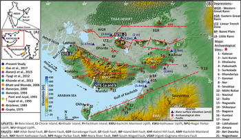
In the inset map of India and (A) Gulf of Kachchh region, the colored dots mark the locations of various studies. The red rectangle marks the location of the enlarged map. (B) Digital Elevation Map of Kachchh peninsula showing major and minor thrusts (modified after Biswas, Reference Biswas2016). Sites investigated in the present study are marked in white circles: the Kharod Estuary (Site-1a), the river section (Site-1b), the India Bridge section (Site-2), and the Nani Cher Estuary section (Site-3). (For interpretation of the references to color in this figure legend, the reader is referred to the web version of this article.)

Holocene sea level influenced and helped sustain coastal communities and contemporary human civilizations (Stanley and Warne, Reference Stanley and Warne1997; Day et al., Reference Day, Gunn, Folan, Yanez-Arancibia and Horton2007; Lawler, Reference Lawler2011). Particularly, the decrease in Mid-Holocene sea level enabled some populations to exploit the exposed coastal lowland environments for sustenance, human migration, and trade (Stanley and Warne, Reference Stanley and Warne1997; Fleming et al., Reference Fleming, Johnston, Zwartz, Yokoyama, Lambeck and Chappell1998). This led to the suggestion of a possible link between the sea-level changes and contemporary human events (e.g., Stanley and Warne, Reference Stanley and Warne1997; Kennett et al., Reference Kennett, Kennett, Erlandson and Cannariato2007). In the Indian context, the western Indian coastal Bronze Age Harappan (Indus Valley) settlements yielded artifacts like circular Persian Gulf seals, terracotta mummy-like figures, and fragments of greenish-gray stone (chlorite-schist) vessels bearing engraved geometric patterns suggesting cultural contact with the Persian Gulf via a sea route (Rao, Reference Rao and Lahiri2000; Rawat, Reference Rawat, Keller and Pearson2015) during the Mid-Holocene. Similarly, a circular seal bearing the Indus script from Madinat Hamad in Oman (Srivastava, Reference Srivastava1991) and a Harappan black-slipped jar were recovered from coastal sites in Oman (Ajithprasad, Reference Ajithprasad2006) suggesting sea trade and exchange of exotic items during Harappan times (Rawat, Reference Rawat, Keller and Pearson2015). Gujarat has around 40 coastal Harappan sites, of which 30 correspond to the mature urban period and 10 correspond to the late- or post-urban period. Of these 40 sites, 19 are along the coast of Kachchh (including Rann), which makes the area an ideal location for exploring the influence (if any) of Mid-Holocene sea level on the evolution of coastal Harappan settlements.
The present study thus aims to determine the RSL—the change in sea level relative to land at a particular time and site (Shennan, Reference Shennan, Shennan, Long and Horton2015)—from intertidal deposits using multiproxy data (sedimentology, trace elements, organic geochemistry, ichnology, and pollen) supported by optical and radiocarbon dating. The objectives are (i) to ascertain the magnitude and causes of Mid- to Late Holocene RSL changes, and (ii) to assess the influence of Mid- to Late Holocene RSL changes on coastal Harappan settlements.
STUDY AREA
The tectonically active nature of the Kachchh Peninsula is demonstrated by episodic high-magnitude intraplate earthquakes, such as the 1819 Allah Bund earthquake (Mw 7.8), the 1956 Anjar earthquake (Mw 6.1), and the 2001 Bhuj earthquake (Mw 7.6) (Rajendran and Rajendran, Reference Rajendran and Rajendran2002; Mandal et al., Reference Mandal, Rastogi, Satyanarayana and Kousalya2004). It is traversed by east–west trending main faults that are transected by several younger oblique faults (Biswas, Reference Biswas2016) (Fig. 1B).
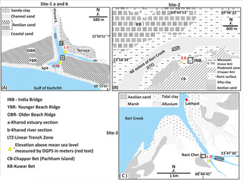
In this study we investigated RSL at three sites; two are located in estuaries (Kharod and Nani Cher) and one is at the distal end of Kori Creek. In the Kharod Estuary (Site-1, located ~200 km east of the Indus delta), two sections (1a and b) have been documented. The Kharod River originates in the southern Katrol Hill Range (KHR) and flows southward for ~60 km before meeting the Gulf of Kachchh (see Figs. 1B and 2A). The river flows through Mesozoic sandstone/limestone/shale, late Cretaceous Deccan basalt, and Tertiary sandstone/shale/laterite and limestone (Maurya et al., Reference Maurya, Thakkar and Chamyal2003). The India Bridge (INB, Site-2) is located at the northern terminus of the linear trench zone (Roy and Merh, Reference Roy and Merh1982) (see Figs. 1B and 2B) and is considered as the farthest relict inland extension of Kori Creek. The rocky Mesozoic hills of Kunwar Bet flank it in the west, and the piedmont zone of Chappar Bet is in the east. Additionally, for broader spatial coverage, an archaeological mound near Nani Cher Estuary (Site-3), at the eastern flank of Kori Creek and ~70 km east of the Indus delta, is also explored. It is inundated during high tides (see Figs. 1B and 2C).
(color online) Geomorphological maps of Site-1a (Kharod Estuary section), Site-1b (Kharod River section), Site-2 (Indian Bridge), and Site-3 (Nani Cher).

Geomorphological settings
In a tide-dominated coastline like the Gulf of Kachchh, a typical tidal-flat profile in the landward direction consists of a lower intertidal sand flat, a middle intertidal mixed sand-mud flat, and an upper intertidal mudflat (Desjardins et al., Reference Desjardins, Buatois and Màngano2012). The relict intertidal flats are preserved in the spit-sheltered location of the tide-dominated Kharod Estuary and the distal end of the gourd-shaped Kori Creek. Such sheltered locations with low tidal amplitudes and restricted wave activity are known to have fine, cohesive deposits from low-energy environments (weak current) and to facilitate gradual deposition of suspended material (Häntzschel, Reference Häntzschel and Trask1955; Lambeck et al., Reference Lambeck, Woodroffe, Antonioli, Anzidei, Gehrels, Laborel, Wright, Church, Woodworth, Aarup and Wilson2010). The absence of lamination further indicates intertidal sedimentation under slackened water conditions during low tidal waters (Semeniuk, Reference Semeniuk and Schwartz2005; Wang, Reference Wang, Davis and Dalrymple2012; Daidu et al., Reference Daidu, Yuan and Min2013). The alongshore current is from the west (Indus delta) to east (Gulf of Kachchh) and is responsible for the dispersion of suspended sediment in the Gulf of Kachchh (see Fig. 1B) (Ramaswamy et al., Reference Ramaswamy, Nath, Vethamony and Illangovan2007).
Geomorphologically, the funnel-mouth estuary setting of the Kharod River is located in a spit and cuspate foreland complex (Kar, Reference Kar1993). In the estuarine zone, dissected southwest–northeast trending coastal dune (beach) ridges are preserved, whereas relict incised mudflats overlying the fluvial sediments form a conspicuous tableland topography (see Fig. 2, Site-1b). It is a mesotidal zone with an average high tidal range of ~2.70 m and an average low tide of ~0.90 m (Unnikrishnan et al., Reference Unnikrishnan, Gouveia and Vethamony1999; Vethamony and Babu, Reference Vethamony and Babu2010). The modern and relict mudflats in the inner estuary flank the main channel axis.
The linear trench zone, in the vicinity of Site-2 (see Fig. 2), experiences spatial and temporal variability in the magnitude and extent of tidal inundation. For example, the southwestern part that lies close to Kori Creek is perennially under tidal inundation; the central part gets inundated during high tide, whereas the northeastern part around the Mesozoic rock–dominated Kunwar Bet gets flooded only during the exceptionally high monsoon wind–driven tidal surges (Glennie and Evans, Reference Glennie and Evans1976; Roy and Merh, Reference Roy and Merh1982; Tyagi et al., Reference Tyagi, Shukla, Bhushan, Thakker, Thakkar and Juyal2012).
METHODOLOGY
The sedimentary sequences were documented and sampled to infer different depositional environments. Samples from units suggesting transitional depositional environments were chosen for geochemical and palynological analyses. Additionally, the intertidal deposits, which are used as sea-level indicators and index points (SLIPs), are characterized using multiproxy data.
Stratigraphy and sedimentology
At Site-1 (eastern flank of the Kharod River), two sections were excavated: the Kharod Estuary section (Site-1a) at the estuary mouth, and the Kharod fluvial section (Site-1b) located ~1 km further inland (see Fig. 2B). At the India Bridge (INB) section (Site-2), the stratigraphy was reconstructed from a trench after excavating through an elevated sandy mound (locally known as sandy Bet) and the Rann surface (see Fig. 2B). At Site-3, the Nani Cher archaeological mound was excavated on the left bank of the Nani Cher Estuary (see Fig. 2C). Data were collected describing sediment composition, texture (grain size), structures, and trace fossils in the measured units. All the elevations of the modern tidal-flat surfaces and studied sections were measured using differential global positioning system (DGPS) with an accuracy of ± 0.01 m. The cross-sectional profiles were made using Total Station with an accuracy of ± 0.03 m.
Grain size analysis was done on Sites 1 and 2 for sandy horizons to support field-based sedimentological observations and to characterize different depositional environments. Samples were dry sieved in a Retsch sieve shaker to obtain various size fractions. The statistical parameters (mean grain size, sorting, kurtosis, and skewness) were computed using the GRADISTAT program (Supplementary Table S1). From the INB section (Site-2), 9 samples from units-III and -IV and 10 samples (except pebbly sandy unit-I) from the Kharod Estuary section were analyzed for grain size.
Carbon, nitrogen, and C/N ratios analyses
The Corg and C/N ratio in tidal-flat/estuarine sediments are governed by the autochthonous (indigenous plants) and allochthonous contributions from the river catchment (Sampei et al., Reference Sampei, Matsumoto, Kamei and Tokuoka1997; Allen et al., Reference Allen, Angela and Drak2007). To characterize and differentiate between the tidal and fluvial environments, 21 samples (U-II and -III) from the Kharod Estuary section (Site-1a), 7 samples from the Kharod River section (U-IV and -V, Site-1b), and 24 samples from INB section (U-I to -IV, Site-2) were analyzed using a Thermo Scientific Flash 2000 Elemental Analyser. The standards used for calibration were low organic content soil containing 1.65% carbon and 0.14% nitrogen. Higher C/N ratios in the tidal-flat environment suggest an increased proportion of river-imported detritus, and lower C/N ratios suggest proportionately more algae and less organic material from fluvial/terrestrial sources (Allen et al., Reference Allen, Angela and Drak2007). Also, plants in general have higher C/N ratios than animals due to their low protein and high cellulose content. Therefore, the autochthonous component contributed by aquatic organisms, algae, and phytoplankton has a C/N ratio ranging from 4 to 10. The allochthonous constituent (mostly coming from terrestrial plants) is more refractory due to their high lignin and cellulose content and has a C/N ratio >12 (Ku et al., Reference Ku, Chen and Liu2005; Nazneen and Raju, Reference Nazneen and Raju2017).
Geochemical analysis
The trace element geochemistry, including rare earth elements (REEs), is used to ascertain temporal changes in the sediment provenance (McLennan, Reference McLennan1993). In total, 28 samples from the Kharod Estuary section (Site-1a, unit-II [9 samples] and unit-III [12 samples]), and Kharod River section (Site-1b, unit-V [7 samples]) were analyzed. In addition, modern intertidal sediments and Kharod River catchment lithology (basalt and sandstone) were also analyzed for comparison with the relict sediment.
Samples were washed in deionized water to remove the salt and were powdered using a planetary ball mill. Following this, the samples were treated with 10% HCl to remove the carbonate. Samples of approximately 300 mg each were digested using Savillex Teflon vials with ultra-pure HF-HNO3 acids in a microwave-assisted digestion system. The final solutions were prepared in 2% HNO3 acid. The analysis was done following the standard protocol in an inductively coupled plasma-mass spectrometry model iCAP-Q from Thermofisher (Ray and Shukla, Reference Ray and Shukla2018). The U.S. Geological Survey geological rock standard BHVO-2 was used for generating the calibration curves, and a laboratory standard (NOVA) was used as the unknown standard. A reproducibility check for trace elements was performed on repeated analyses on a different set of aliquots of BHVO-2 standard, which is better than 3% at the 2-sigma level.
The trace-element data, including REEs, were normalized with the upper continental crust composition (Taylor and McLennan, Reference Taylor and McLennan1985). To ascertain probable sediment contribution into the Kharod Estuary, the geochemical data are compared with the Kharod River catchment dominant basalt lithology, modern intertidal sediments, and the Indus Delta sediments from Keti Bunder (Clift et al., Reference Clift, Giosan, Carter, Garzanti, Galy, Tabrez and Pringle2010).
Trace fossils (ichnology) and palynological analysis
To further understand the nature of the depositional environment, the excavated sediment sections were investigated for trace fossils. The centimeter-scale, serial sectioning technique was used to identify trace fossil morphology following Häntzschel (Reference Häntzschel and Teichert1975) and Knaust (Reference Knaust2017). Documented trace fossils were mostly vertical to sub-horizontal, with higher clay content. In order to ascertain the precise nature of the depositional environment, the trace fossil data are compared with the modern analog of the site—the proximal Mandvi intertidal zone (Patel and Desai, Reference Patel and Desai2009).
For the palynological study, 10 samples from unit-III of the Kharod Estuary section (Site-1a), 4 samples from unit-V of the Kharod River section (Site-1b), and 4 samples from unit-I of the INB section (Site-2) were collected. The Nani Cher section (Site-3) is dominated by the sand fraction, and therefore it was not used for palynological study. Sediment samples of about 10 g were prepared following standard pollen analytical techniques, including acetolysis (Erdtman, Reference Erdtman1943). Sample residues were mounted on microscope slides in a glycerine jelly medium. Pollen grains and fern spores were identified to the lowest possible taxonomic level using the Birbal Sahni Institute of Palaeosciences museum collection of reference pollen and published pollen keys (Thanikaimoni, Reference Thanikaimoni1987; Nayar, Reference Nayar1990). The pollen counts were made with the help of an Olympus microscope at a magnification of 400×. Most of the pollen samples were counted to a minimum of 150 grains.
CHRONOLOGY
Twelve samples were dated using the optically stimulated luminescence (OSL) technique. The OSL dating technique exploits the radiation dosimetric properties of mineral grains (usually quartz and feldspar). The energy from natural radioisotopes in the sediment is absorbed and stored in the crystal lattice of minerals that may be released as luminescence upon excitation/heating. It relies on the premise that the geological luminescence of samples is bleached to near residual levels during transportation and begins to accumulate once the sediment is deposited (Aitken, Reference Aitken1998). The samples were collected in specially designed opaque metal pipes, and the pure quartz was extracted by sequential pre-treatment with 10% HCl and 30% H2O2, respectively. The dried samples were sieved to obtain a 90–150 μm size fraction. Additionally, the quartz grains were checked for feldspar contamination by subjecting them to infrared stimulated luminescence (IRSL). The equivalent doses (De) were measured using a modified (double) single aliquot regeneration protocol (SAR; Murray and Wintle, Reference Murray and Wintle2000; Banerjee et al., Reference Banerjee, Murray, Bøtter-Jensen and Lang2001) except for two samples for which the RSL count was near background and the SAR protocol was used (Murray and Wintle, Reference Murray and Wintle2000). The luminescence measurements of the quartz extract were carried out in an automated Risø TL-OSL reader (TL/OSL-DA-20; Bøtter-Jensen et al., Reference Bøtter-Jensen, Thomsen and Jain2010). The samples were stimulated using a blue diode (470 ± 20 nm) and detected with an EMI 9835 QA photomultiplier tube coupled with a 7.5–mm Hoya U-340 filter (emission 330 ± 35 nm). An on-plate 90Sr/90Y beta source was used for beta irradiations. Typically, around 90 aliquots were analyzed, out of which 16–47 aliquots satisfied the criterion of a recycling ratio of 0.90–1.1 and were used for computing the De values. The growth curve, IRSL, shine down curve, and abanico plots showing the De distribution of each dated sample is given in the supplementary data (Supplementary Figs. S1–S3). For radioactivity, the concentrations of uranium, thorium, and potassium were measured in the high purity germanium detector (HPGe). The samples were sealed in plastic boxes and kept for ~15 days to attain radioactive equilibrium. The concentrations were estimated based on the characteristic gamma rays using a standard basalt reference source (107). The errors of measurement (systematic and statistical uncertainties) are <5% (Shukla et al., Reference Shukla, Bhandari and Shukla2002). The appropriate statistical model, such as the Central Age Model (CAM) or the Minimum Age Models (MAM)-3/4, are chosen for the computation of De that is based upon the statistical parameters like over-dispersion (OD), skewness, and kurtosis (Bailey and Arnold, Reference Bailey and Arnold2006; Galbraith and Roberts, Reference Galbraith and Roberts2012). The CAM is preferred if the OD is ≤40%, where OD as a criterion is usually sufficient to choose between CAM and MAM (Bailey and Arnold, Reference Bailey and Arnold2006). This further suggests that sediments were adequately bleached (Galbraith and Roberts, Reference Galbraith and Roberts2012). Following the same criteria, we employed CAM for the computation of De values in R (calc_Central Dose) using the script of Burow (Reference Burow2019). The ages were computed using the java-based dose rate and age calculator (DRAC), which also calculates the contribution from cosmic rays at a given location (Durcan et al., Reference Durcan, King and Duller2015). An average water content of 10 ± 5% was used (Fuchs et al., Reference Fuchs, Gloaguen, Krbetschek and Szulc2014).
In addition to this, two carbonate intertidal shell samples were radiocarbon dated and the radiocarbon activity was measured in a liquid scintillation counter “LKB-QUANTULUS” (Yadava and Ramesh, Reference Yadava and Ramesh1999). The samples were collected from the same horizons, which were also optically dated so that ages may be corroborated for consistency and reliability. Furthermore, it has been observed that the dead carbon effect (continental contamination) is expected to be minimal as the shells are collected from intertidal deposits with no restriction in water circulation (Hogg et al., Reference Hogg, Higham and Dahm1998; Bezerra et al., Reference Bezerra, Vita-Finzi and Lima Filho2000). The radiocarbon ages were calibrated using the Calib7.1.0 program and the Marine13 data set (Stuiver and Reimer, Reference Stuiver and Reimer1993; Reimer et al., Reference Reimer, Bard, Bayliss, Beck, Blackwell, Ramsey and Buck2013). The average marine reservoir age (ΔR ± σ 135 ± 86 years) of three proximal locations (map no. 606-Pirotan Island, 591-Port Okha, and 592-Dwarka) was taken for reservoir age correction (Bhushan et al., Reference Bhushan, Chakraborty and Krishnaswami1994; Dutta et al., Reference Dutta, Bhushan and Somayajulu2001) in the Calib7.1.0 program.
Sea-Level Index Point (SLIP) and RSL change
RSL change is used to quantify the change in sea level at a particular time and site relative to a land-based reference frame of the present (Shennan, Reference Shennan, Shennan, Long and Horton2015; Rovere et al., Reference Rovere, Raymo, Vacchi, Lorscheid, Stocchi, Gomez-Pujol, Harris, Casella, O'Leary and Hearty2016). Based on multiple proxies, the intertidal deposits are characterized as lower, middle, and upper intertidal deposits. The upper intertidal deposits are formed between Mean High Water Spring (MHWS) and Mean High Water Neap (MHWN); middle intertidal deposits are formed between Mean High Water Neap (MHWN) and Mean Low Water Neap (MLWN); and the lower intertidal deposits are formed between the Mean Low Water Neap (MLWN) and Mean Low Water Spring (MLWS) (Daidu et al., Reference Daidu, Yuan and Min2013).
For a sea-level indicator to be identified as a SLIP, it must have the following well-constrained attributes: location, age, indicative meaning, and tendency (Shennan, Reference Shennan, Shennan, Long and Horton2015; Vacchi et al., Reference Vacchi, Engelhart, Nikitina, Ashe, Peltier, Roy, Kopp and Horton2018). Where the data points (both terrestrial and marine) could not be compared directly with the past tide levels, we ascribed these as limiting data points (Shennan and Horton, Reference Shennan and Horton2002). We used in situ, well-dated, relict intertidal deposits as SLIPs to calculate RSL changes, where RSL change is the elevation difference of the SLIP with respect to its modern analog (Shennan, Reference Shennan, Shennan, Long and Horton2015). Here elevation (amsl) of the SLIP is denoted by (Es), and elevation of the modern analog with reference to a tidal level is called the Reference Water Level (RWL). The range over which RWL varies is known as the Indicative Range (IR). The RWL (amsl) was estimated by taking the mean of n points at three corresponding locations (Supplementary Tables S2–S4). The IR (amsl) is at a 95% confidence interval and 1.96 times the standard deviation (Shennan et al., Reference Shennan, Long and Horton2015). As suggested by Hijma et al. (Reference Hijma, Engelhart, Törnqvist, Horton, Hu, Hill, Shennan, Long and Horton2015), the errors were calculated by taking into account the IR error, DGPS error, sampling unit thickness error, vertical exposure error, variance in RWL, and variance of SLIP elevation (see Supplementary Table S1).
The RSL change was calculated using the respective modern analogs (Table 1) using statistically computed IR (see Supplementary Table S1). For comparison, the RSL was also estimated using IR determined from the various tidal ranges available at Okha tidal gauge station (see Fig. 1, Table 2), because the site proximal stations (Mandavi and Jhakau) have no record of MLWS, MHWS, MHWN, and MLWN (see Table 2). The absolute RSL values vary within the error limits (see Table 1), and hence we used the statistical IR for RSL estimation.
Details of intertidal deposits and the chronology that are used as SLIPS (Sea-Level Index Points). For comparison we give RSL estimates from two indicative ranges (IR1 and IR2) following the same protocol (for details see Supplementary Tables S1–S3). RSL1 is estimated using IR1, and RSL2 is estimated using IR2. As can be seen, the RSL does not vary significantly (it fluctuates within the errors). Average RSL values are calculated and corrected for tectonic component from RSL1. All values are in meters above mean sea level (m amsl). At the Kharod Estuary/river and IB sections the uplift rates are 0.13 ± 0.01 mm/yr and 0.2 ± 0.01 mm/yr, respectively.

Notes: RWL = Reference Water Level; IR1 and IR2 = Indicative Ranges; Es = Elevation of the dated relic intertidal units top; RSL1t and RSL2t = Relative Sea-Level change with tectonic overprinting; RSL1 and RSL2 = Relative Sea-Level change without tectonic overprinting; MLWN = Mean Low Water Neap; MLWS = Mean Low Water Spring; MHWS = Mean High Water Spring; and MHWN = Mean High Water Neap.
Tide gauge data recorded at the mouth of the Gulf of Kachchh near Okha (west and southwest of the studied sites) (Babu et al., 2005), Mandavi (near Kharod Estuary), and Jakahu port near Kori Creek (Gujarat Maritime Board).

Notes: MHWS = Mean High Water Spring, MHWN = Mean High Water Neap, MLWN = Mean Low Water Neap, MLWS = Mean Low Water Spring, MSL = Mean Sea Level, HHW = Higher High Water, MHHW = Mean Higher High Water, MLHW = Mean Low Higher Water, MHLW = Mean High Low Water, and MLLW = Mean Lower Low Water.
RESULTS
Stratigraphy
Site-1a (Kharod Estuary section, 22.845093°N, 69.229249°E)
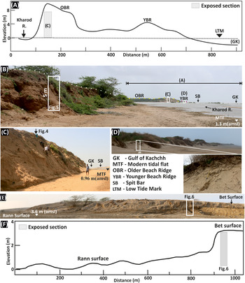
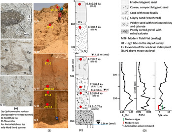
An ~6–m–thick sediment sequence is exposed along the left flank of the tidal creek (see Figs. 2A, 3C, and 4). The elevation of the modern tidal surface is 0.96 m amsl. Based on the sediment texture and degree of weathering, five sedimentary units have been identified (see Fig. 4). The lowermost ~30–cm-thick unit- I is composed of faintly cross-laminated, angular to sub-rounded, pebbly quartz-rich, reddish-yellow sand containing subordinate basalt fragments and rolled calcretes. This is followed by the ~40–cm-thick unit-II, which contains pebbly sand mixed with subordinate (translocated) clay coating and angular to sub-rounded calcrete. Overlying this is the ~75–cm-thick unit-III of which the lower 35 cm is massive, compact, and weathered clayey-sand and the upper 40 cm is a sandy horizon that contains trace fossils (see Fig. 4A). Grain-size analysis shows the dominance of poorly sorted fine sand that is fine (positively) skewed (see Supplementary Table S1). The trace fossils include Ophiomorpha nodosa, Polykladichnus isp., Planolites isp, Skolithos isp, and a mud-lined burrow (see Fig. 4A). This is succeeded by the ~250–cm-thick unit-IV, which is compact, coarse, biogenic sand containing mica and randomly dispersed friable, tubular calcretes whose concentration increases upwards. Grain-size analysis shows the dominance of fine, moderately well to moderately sorted and finely skewed sand (see Supplementary Table S1). The ~200–cm-thick unit-V, which is micaceous, biogenic sand with insignificant friable calcrete concretions, overlies this unit (see Fig. 4). The grain size data indicate dominance of fine, moderately well-sorted and finely skewed sand that becomes very coarse (negatively) skewed to very finely skewed toward the top (see Supplementary Table S1).
(color online) (A) Cross-section profile generated using Total Station survey data from the Gulf of Kachchh (GK) to the Kharod River section. Low tide mark (LTM) elevation as of April 7, 2017. (B) Field photograph showing locations of Kharod River and estuary sections (Site-1a and Site-1b). (C) Field photographs of the Kharod Estuary and (D) younger beach ridge (YBR) with close-up. (E)–(F) Field photos and cross-section profile at Site-2 near India Bridge.

(A) Close-ups of trace fossils and mud-lined burrow (mlb), which are filled with passive sediments from the upper bioturbated section of unit-III. (B) Close-up of Kharod Estuary section with optically stimulated luminescence (OSL) sample locations (red circles). (C) The stratigraphic details along with the OSL ages. The average differential global positioning system (DGPS) elevation of the modern lower intertidal flat (n = 30) corresponds to Mean Low Water Spring (MLWS) and Mean Low Water Neap (MLWN) range. The high tide (HT) is the level of high tide marked on the day of survey (April). (D) Corg, Ntotal, and C/N ratio obtained on unit-II and -III indicate dominance of marine organic matter. (For interpretation of the references to color in this figure legend, the reader is referred to the web version of this article.)

Site-1b (Kharod River section, 22.857521°N, 69.228848°E)
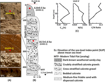
An ~4.5–m-thick alluvial sequence is exposed along the left bank of the Kharod River (see Figs. 2A, 3B, and 5) where modern tidal flats are 1.3 m amsl. Based on the sediment texture and structures, five broad sedimentary units (base unexposed) have been identified (see Fig. 5). From bottom upwards, unit-I (30 cm) is dominated by medium to fine friable sand containing dispersed calcretes. Unit-II contains ~40-cm-thick bedded calcretes with subordinate rolled calcrete nodules. This unit is weathered and laterally persistent along the river to a distance of ~500 m (see Fig. 3B). It is overlain by unit-III, which is ~100 cm thick and composed of cross-stratified (planar and trough) calcrete gravel. The bedding attitude (azimuths) of the cross-stratification exhibits strike of east–west (90–270°) to east-southeast–west-northwest (95–275°) and dips gently toward the south (180°) to south-southwest (185°). The overlying ~200-cm-thick unit-IV contains crudely stratified rounded to sub-rounded calcrete gravels, subordinate basalt lithoclasts, and impersistent sand lenses. The uppermost 75-cm-thick unit-V is dominated by weathered dark brown massive and fractured sandy-clay with a sharp basal contact (see Fig. 5), which forms a well-defined terrace surface around the Kharod Estuary (see Fig. 2A).
(A) Close-up field photographs of the Kharod River section with location of optically stimulated luminescence (OSL) samples (red circles). (B) Stratigraphic details along with the OSL ages. The average differential global positioning system (DGPS) elevation of the modern middle tidal flat (n = 20) corresponds to Mean Low Water Neap (MLWN) and Mean High Water Neap (MHWN). (C) Corg, Ntotal, and C/N ratio indicate dominance of marine organic matter. (For interpretation of the references to color in this figure legend, the reader is referred to the web version of this article.)

Site-2 (India Bridge section, 23.977750°N, 69.757433°E)
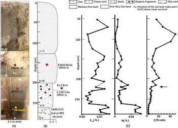
This site is located ~70 km inland in the distal linear trench zone of Kori Creek (Gulf of Kachchh) and is 3.6 m amsl (see Figs. 1 and 2C). The stratigraphy is reconstructed from an ~3–m-deep trench excavated at the western margin of Chappar Bet (see Figs. 3E and 6). The lowermost 30–cm-thick unit-I is composed of dark gray sticky clay containing gastropod shells (Melania striatella tuberculata). This is followed by 60 cm of thick clayey-sand containing shells and bioclast fragments (unit-II). The sticky clay is gradually replaced by medium to fine silty-sand in the upper part. The overlying ~70-cm-thick unit-III is dominated by poorly to moderately sorted fine sand that is coarsely skewed toward the top (see Supplementary Table S1). The uppermost ~125-cm-thick unit-IV is massive fine to very fine moderately well-sorted sand (see Supplementary Table S1) containing bioclast fragments (see Fig. 6). The sandy units are devoid of mica.
(A) Close-up field photograph of the India Bridge (INB) sediment profile, optically stimulated luminescence (OSL) samples (red circles), and radiocarbon locations samples (yellow circle). The average differential global positioning system (DGPS) elevation (n = 6) of the modern upper tidal flat at Sunda High (white inverted triangle) corresponds to Mean High Water Spring (MHWS) and Mean High Water Neap (MHWN) range. (B) Stratigraphy details along with the OSL ages. Es is also marked considering the low (marine) C/N ratio. (C) Note that units-I and -II showing low Corg, C/N ratio, and relatively high Ntotal suggesting deposition under a distal intertidal environment. Black arrow marks the break in trend (increased aeolian influence). (For interpretation of the references to color in this figure legend, the reader is referred to the web version of this article.)

Site-3 (Nani Cher Archaeological mound, 23.795944°N, 68.678600°E)
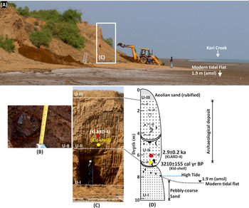
The archaeological mound with underlying alluvium is excavated along the eastern flank of the Nani Cher Estuary (see Fig. 2C) in which three broad stratigraphic units were identified (Fig. 7). The modern tidal flat is 1.9 m amsl at this location. From bottom upwards, the lowermost ~300-cm-thick unit-I is dominated by pebbly-coarse sand containing occasional charcoal and potsherds. Unit-I continues below the modern tidal flat that abuts it (see Fig. 7). This is overlain by the ~400-cm-thick unit-II, which is dominated by randomly dispersed archaeological deposits such as iron slag, ash layers, potsherds, bones, shells, and bangles. At places, the unit is punctuated by channel activity, which is represented by lenticular sand layers overlain by clayey-silt. The archaeological mound is covered with the rubified aeolian sand (unit-III) (see Fig. 7).
(A) Field photograph showing the panoramic view of Nani Cher Estuary, location of the section excavated is shown by a white rectangle. (B) Close-up of unit-II showing iron slag in archaeological deposit. (C) Field photograph and (D) stratigraphic details of the section. Note that unit-I continues below the modern intertidal flat. The radiocarbon age (yellow circle) of 3210 ± 155 cal yr BP (Kld-shell) is obtained on Turbinella pyrum (conch shell) collected ~60 cm above the high tide (HT) (May 2017), and the sediment sample (red circle) is dated to 2.9 ± 0.2 ka. (For interpretation of the references to color in this figure legend, the reader is referred to the web version of this article.)

Carbonorg (Corg), Nitrogen (Ntotal), and C/N ratios
In the Kharod Estuary section (Site-1a), the Ntotal and Corg has a declining trend toward the top, whereas the C/N ratio shows an increasing trend from mid-unit-III (see Fig. 4D, Supplementary Table S5). The C/N ratios for the modern clay and algae are 4.0 and 5.6, respectively (see Supplementary Table S5). In the Kharod River section (Site-1b), Ntotal shows an increasing and then decreasing trend, while the Corg is has an increasing trend. The C/N ratio preferentially increases toward the top (see Fig. 5C). In the INB (Site-2) section, Ntotal has its highest concentration at the bottom, Corg has its highest concentration in unit-I and its lowest concentration in unit-II and unit-IV, and the C/N ratio has an overall increasing trend toward the top (see Fig. 6C, Supplementary Table S5).
Trace elements geochemistry
For provenance interpretation, we used the average values of the trace element data that were generated from 21 samples from Site-1a (Kharod Estuary section, units-II and -III), 7 samples from Site-1b (Kharod River section, unit-V), modern intertidal sediments, and the catchment's dominant lithology samples (basalt and sandstone) (Fig. 8, Table 3).
(color online) The plot of upper continental Crust (UCC) (Taylor and McLennan, Reference Taylor and McLennan1985) normalized trace elements from the Kharod Estuary section (units-II and -III), Kharod River section (unit-V), and modern tidal clay. The normalized trace element values of Kharod River catchment lithology (basalt) and the Indus delta sediments (Keti Bunder; Clift et al., Reference Clift, Giosan, Carter, Garzanti, Galy, Tabrez and Pringle2010) are also shown.

Average values of trace element concentrations from dominant lithology, modern intertidal sediments, and different sedimentary units plotted in Figure 8 are given. The range of concentration is given in parentheses.

Trace fossils and palynological evidence
The trace fossils Ophiomorpha nodosa, Polykladichnus isp., Planolites isp., and Skolithos isp. and mud-lined burrows (see Fig. 4) dominate unit-III in the Kharod Estuary section (Site-1a). Ophiomorpha nodosa occurs as a thick nodose walled burrow, elliptical in cross section, 14 cm in diameter and was made by a suspension-feeding trace maker like Oratosquilla striata (Patel and Desai, Reference Patel and Desai2009). Polykladichnus isp. occurs as vertical to inclined Y-shaped burrow made by a suspension-feeding trace maker. Planolites isp. occurs as a circular to elliptical cross section of the horizontal burrow with active burrow filling made by deposit-feeding trace makers. Skolithos isp. is a vertically oriented unbranched burrow of suspension-feeding trace makers (Patel and Desai, Reference Patel and Desai2009). Many modern crustaceans commonly make mud-lined burrows by inserting pellets along burrow walls.
No pollen spores were recovered from the Kharod Estuary (Site-1a) unit-III except for a few fungal spores, which could be due to a higher concentration of sand. Also, there was no significant yield from the INB (Site-2) section. In contrast, the Kharod River section (Site-1b) unit-V yielded mangrove pollen taxa such as Rhizophora mucronata and Avicennia marina. The other mangrove pollens, including Bruguiera and Ceriops, were also present but in lower percentages. The lower part of this unit has a higher representation of R. mucronata (20–35%) and a high concentration of Avicennia (50%). Among the terrestrial taxa, pollen grains of Malvaceae, Prosopis juliflora, and Myrtaceae were recorded in low values. In general, herbs and grasses are consistently present throughout this unit at values ranging from 15% to 30%. The highest presence of herbs and grasses such as Asteraceae, Cyperaceae, Artemisia, Poaceae, and Chenopodiaceae/Amaranthaceae were observed in the upper portion.
Chronology
The fluvial sand facies with translocated tidal clay (unit-II) at the Kharod estuary section (Site-1a) is dated to 9.9 ± 0.7 ka (UNIT-2) and 9.3 ± 0.4 ka (LTL-1). The overlying intertidal unit-III is dated between 7.3 ± 0.4 ka (UNIT-3A) and 4.7 ± 0.2 ka (LTL-2). The upper aeolian beach ridge (unit-IV) is dated to 4.3 ± 0.2 ka (LTL-4), and unit-V is dated to 0.4 ± 0.03 ka (LTL-5) (see Fig. 4, Table 4). The younger (modern) beach ridge is dated to 0.2 ± 0.01 ka (MBR) (see Fig. 3D), which is located ~100 m from the modern shoreline and is ~3 m high. At Kharod fluvial section (Site-1b), the planar stratified gravelly sand (unit-IV) is dated to 16.5 ± 1.6 ka (KHRD-2), and the upper intertidal clay (unit-V) is dated to to 6.8 ± 0.5 ka (KHRD-3) (see Fig. 5). At India Bridge (Site-2), the gastropod shell (Melania stiatella tuberculata) collected from the lowest unit-I is radiocarbon dated to 1045 ± 175 cal yr BP (IB-shell) (see Fig. 6, Table 5). The overlying unit-II is optically dated to 1.1 ± 0.1 ka (IBOSL-1), and the unit-III is dated to 0.8 ± 0.04 ka (IBOSL-2) (see Fig. 6). At Nani Cheri Estuary (Site-3) the Turbinella Pyrum (conch shell) is radiocarbon dated to 3210 ± 155 cal yr BP (Kld-shell) (see Fig. 7, Table 5), and a sandy layer in unit-II is optically dated to 2.9 ± 0.2 ka (KLARD-4). Details of the radioactivity, dose rate, equivalent dose, and the ages obtained are shown in Table 4, and typical growth curves, shine down and IRSL plots, and De distribution are given in Supplementary Figures S1–S3.
Details of the samples, number of aliquots used (N), radioactivity details, over dispersion (OD), central age model (CAM) equivalent dose (De), dose rate, and ages obtained for various landforms. Water content used 10 ± 5% (Fuchs et al., Reference Fuchs, Gloaguen, Krbetschek and Szulc2014).

The radiocarbon ages obtained on samples collected from India Bridge and Nani Cher. The reservoir correction age (ΔR ± σ) was 135 ± 86 years (Bhushan et al., Reference Bhushan, Chakraborty and Krishnaswami1994; Dutta et al., Reference Dutta, Bhushan and Somayajulu2001).

Notes: IB = India Bridge, Kld = Kali Nadi
DISCUSSION
Depositional environment
Site-1a (Kharod Estuary section, 22.845093°N, 69.229249°E)
The lowermost faintly cross-laminated pebbly sandy unit-I can be interpreted as channel lag deposits (Therrien, Reference Therrien2006). Because of the limited space of the river channel, the river repeats stages of erosion and accumulation in the adjacent regions. The overlying pebbly sand containing angular to sub-rounded calcrete with occasional clay coating (unit-II) suggests deposition under a relatively stable fluvial environment (consistent discharge with occasional flooding) (Juyal et al., Reference Juyal, Raj, Maurya, Chamyal and Singhvi2000; Bhattacharya et al., Reference Bhattacharya, Rastogi, Thakkar, Patel and Juyal2014). The clay coating seems to be physically translocated from the overlying unit-III through cracks (see Fig. 4); this is suggested to be the reason for a relatively high concentration of organic carbon and nitrogen in unit-II because clay provides a large surface area and has a higher sorptive capacity (Dunn et al., Reference Dunn, Welsh, Teasdale, Lee, Lemckert and Méziane2008; Nazneen and Raju, Reference Nazneen and Raju2017). The grain-size dependency for carbon and nitrogen is further supported by the modern clay sample from the Kharod estuary, which contains 0.90% C org, 0.22% Ntotal, and a C/N ratio of 4. However, the C/N ratio (except for one point) remains below 10, implying that the organic matter and the nitrogen were largely contributed from marine sources (Bordovskiy, Reference Bordovskiy1965; Prahl et al., Reference Prahl, Bennett and Carpenter1980).
Considering the textural attributes of unit-III (clayey-sand), it can be suggested that it is an intertidal deposit where deposition occurred by a combination of tidal current (deposition of sand) followed by the slackening facilitating the deposition of clay as suspension fall out (Häntzschel, Reference Häntzschel and Trask1955). Further, the absence of lamination suggests sedimentation under a relatively low-energy, lower-intertidal environment (Semeniuk, Reference Semeniuk and Schwartz2005; Wang, Reference Wang, Davis and Dalrymple2012; Daidu et al., Reference Daidu, Yuan and Min2013) and not the subtidal environment that is dominated by coarser sediment having lag-scour structures produced by lateral migration of bedforms under subtidal high energy currents (Dalrymple et al., Reference Dalrymple, Mackay, Ichaso, Choi, Davis and Dalrymple2012; Daidu et al., Reference Daidu, Yuan and Min2013). The possibility of post-depositional erosion is negated, because unit-III can be laterally traced (~1 km toward the coast) with near-uniform thickness and is overlain by aeolian sand (older beach ridge and reworked deposits). Unit-III also has a moderate Bioturbation Index of BI-3 made up of high-density mud-lined burrows of suspension-feeding organisms (e.g., Ophiomorpha nodosa). Construction of mud-lined burrows requires organisms to extract mud from suspension mode and use it to support its burrow walls. In contrast, organisms with deposit feeding will recycle and process the sediment and deposit it as an active burrow fill, thus generating an entirely different morphology of trace fossil. Thus, for the survival of suspension-feeding organisms, water is required to be under agitated conditions to keep the mud and organic matter in suspension mode—a condition usually found in the lower intertidal/subtidal zone (more frequently toward the low water line) (Desai and Patel, Reference Desai and Patel2008; Dalrymple et al., Reference Dalrymple, Mackay, Ichaso, Choi, Davis and Dalrymple2012). Moreover, the Ophiomorpha burrows are absent near the high-tide level/foreshore/backshore area, as the trace maker cannot sustain the environmental stress-induced prolonged exposure between the tides along with heat and lack of water. Similar occurrence of Ophiomorpha from lower intertidal and subtidal zones are also persistent from the Pleistocene-age Dwarka Formation exposed along the southern shores of the Gulf of Kachchh (Desai, Reference Desai2016), and from modern lower intertidal/ subtidal zones along Mandvi to Mundra in the northern shores of the Gulf of Kachchh (Desai and Patel, Reference Desai and Patel2008; Patel and Desai, Reference Patel and Desai2009). Additionally, the ichnozonation model of the tide-dominated depositional profile of Buatois and Màngano, (Reference Buatois and Màngano2011, p. 142) also supports higher/moderate trace fossil diversity and degree of bioturbation in the lower intertidal zone, which decreases significantly in the subtidal zone owing to widespread high energy conditions and scouring (Buatois and Màngano, Reference Buatois and Màngano2011, p. 142). Thus, ichnological diversity and density with BI-3 along with the sedimentological evidence suggests that unit-III was deposited under lower intertidal zone deposits between MLWS and MLWN (Daidu et al., Reference Daidu, Yuan and Min2013).
The overlying, moderately compact well-sorted, very coarse to very finely skewed fine sand corresponding to unit-IV and -V having a variable concentration of broken shell fragments, indicate transportation by winds from near coastal environments (source proximal). The overlying coarse to moderately skewed fine sand with dispersed broken shells suggests sub-recent accretion by coastal winds and deposition as linear hummocky mounds, similar to the coastal dunes/beach ridges in a prograding coastline (Compton and Franceschini, Reference Compton and Franceschini2005). Johnson (Reference Johnson1919), was the first to describe beach ridges in the geological literature and considered these to be constructed by waves along successive shore positions. The beach ridges are narrow, sub-parallel, relict fore dunes of strand plains (Otvos, Reference Otvos2000). These are formed by a combination of waves and winds in areas having an abundance of sediment supply with low offshore gradient and can be used to reconstruct RSL (Taylor and Stone, Reference Taylor and Stone1996). The typical morphology is ascribed to vegetation that forms at the upper limit of swash, and the ridge growth is accomplished by aeolian deposition (Hesp, Reference Hesp and Thom1984). The beach ridges thus are defined as relict, semi-parallel, multiple wave- and wind-built landforms that originated in the inter- and supra-tidal zones. It is suggested that since the Mid-Holocene RSL, beach ridges prograded episodically seaward (Tankard and Rogers, Reference Tankard and Rogers1978; Otvos, Reference Otvos2000). Thus, the presence of two distinct beach ridges around the Kharod estuary can be interpreted as a gradual recession of the sea (see Fig. 3A).
Site-1b (Kharod River section, 22.857521°N, 69.228848°E)
The well-sorted, medium-fine sand in the lowermost unit-I suggests deposition proximal to the trunk channel by a low-energy meandering fluvial system (Goudie, Reference Goudie, Goudie and Pye1983; Willis and Behrensmeyer, Reference Willis and Behrensmeyer1994). The overlying and laterally persistent bedded calcrete (unit-II) indicates the upward migration of carbonate-rich subsurface water along the riverbanks (the channel proximal to the riverine playa environment) during periods of prolonged dryness (Goudie, Reference Goudie, Goudie and Pye1983). Such a geomorphic setting, coupled with dry climatic conditions, favored the development of bedded calcretes due to the evaporation-controlled fluctuations in the ground water (McCarthy and Metcalfe, Reference McCarthy and Metcalfe1990).
The cross- and trough-stratified rolled calcrete–dominated horizon (unit-III) and the crudely stratified rounded to sub-rounded calcrete gravels (unit-IV) suggest episodic mobilization of unconsolidated bed material during the occasional intense rainfall events (Reid and Frostick, Reference Reid, Frostick and Thomas1997). Dominance of rolled calcrete implies a poorly vegetated river catchment that facilitated the erosion of pre-existing alluvial carbonates by frequent channel migration (bank undercutting and collapse). The decreasing amplitude of trough cross beds in the upper part suggests declining flow through time (Miall, Reference Miall1977; Juyal et al., Reference Juyal, Raj, Maurya, Chamyal and Singhvi2000). The large variability in the grain size in units-III and -IV (sand to gravel) could be due to the high bed load transport rates and infrequent short-lived floods (Nanson and Tooth, Reference Nanson, Tooth, Singhvi and Derbyshire1999; Tooth, Reference Tooth2000).
The uppermost massive, fractured dark brown sandy-clay (unit-V) indicates deposition dominantly under suspension that falls out away from the tidal channel in the middle tidal regime (Dalrymple et al., Reference Dalrymple, Mackay, Ichaso, Choi, Davis and Dalrymple2012; Rick et al., Reference Rick, James, Daidu, George, Hui-Ling and Ting-Ting2017). The low C/N ratio (<10) (see Fig. 5C) implies that the organic matter and the nitrogen were largely contributed from the marine source (Bordovskiy, Reference Bordovskiy1965; Prahl et al., Reference Prahl, Bennett and Carpenter1980). The presence of Rhizophora mucronata in the lower part of unit-V suggests that the site was inundated by tidal flooding, whereas the appearance of Avicennia marina in the upper part points toward the declining tidal influence (Banerji et al., Reference Banerji, Pandey, Bhushan and Juyal2015). The intertidal deposits are located ~1 km inland, indicating frequent tidal inundation with a decrease in the tidal influence and suggesting gradual change toward the middle intertidal zone.
Site-2 (India Bridge section, 23.977750°N, 69.757433°E)
Texturally, gray sticky tidal clay (unit-I) with intact gastropod shells (Melania striatella tuberculata) suggests low-energy conditions, which facilitated the deposition of clay as a suspension fall out (Christiansen et al., Reference Christiansen, Vølund, Lund-Hansen and Bartholdy2006) in a distal/upper tidal-flat environment (Tyagi et al., Reference Tyagi, Shukla, Bhushan, Thakker, Thakkar and Juyal2012). The overlying, clayey-sand (unit-II) suggests gradual withdrawal of the distal tidal-flat sedimentation and contribution of aeolian sand from the proximal areas. Both unit-I and unit-II have relatively high Corg and Ntotal, and the C/N is <10, thus suggesting deposition under an intertidal environment. The overlying less fine to very fine, moderately well-sorted sand units (III and IV) (see Supplementary Table S1) indicate deposition as a source proximal obstacle aeolian sand sheet (see Fig. 6).
Site-3 (Nani Cher Archaeological mound, 23.795944°N, 68.678600°E)
The dominance of coarse pebbly sand at the lowermost unit-I suggests mobilization of coarse detritus from the surrounding upland (via fluvial channel activity) during the low stand. The bottom of this unit extends below the modern tidal flat, further suggesting that deposition occurred during lower sea level compared to the present. The overlying archaeological deposit (unit-II) indicates human occupation. The topmost rubified aeolian sand (unit-III) can be interpreted as deposition under drier conditions.
Sediment provenance
The trace element plots (see Fig. 8) show that the trend for Site-1a (estuary, unit-III), Site-1b (river section, unit-V), and the modern intertidal clay closely follow the Indus delta sediments trend. The Indus delta sediments are thought to have been routed by the alongshore current toward the Gulf of Kachchh (Ramaswamy et al., Reference Ramaswamy, Nath, Vethamony and Illangovan2007; Ferrier et al., Reference Ferrier, Mitrovica, Giosan and Clift2015). Similarly, unit-II of Site-1a also follows the Indus delta trend because there is a significant contribution of the translocated clay from the overlying unit-III. However, as can be seen, the Indus delta sediments have high elemental concentrations, which can be attributed to the size-sorting effect (McLennan, Reference McLennan1993), whereas the enriched Sr in modern sediments can be attributed to the greater influence of seawater. The contribution from the primary rock basalt in the river catchment can also be observed in the REEs from Nd to Lu. The mixing of the source sediment seems reasonable in intertidal deposits as sediment is derived from both the continent and sea. The trend of sandstone is not plotted given the low concentration of REE and its derivation from the primary igneous rock basalt.
Estimation of RSL
Sedimentology, geochemistry, trace fossils, C/N ratios, and palynological evidence are used to demonstrate that the clayey deposits (unit-III at Site-1a [Kharod Estuary], unit-V at Site-1b [Kharod River section], and units-I and -II at INB [Site-2]), were deposited under intertidal environments (discussed above), and are used to estimate the RSL changes.
At the Kharod Estuary (Site-1a), the top of the lower intertidal deposits (unit-III, 4.7 ± 0.2 ka) is taken as the marine limiting data point and the bottom (7.3 ± 0.4 ka) is taken as the SLIP at 2.38 m amsl (Es). The beach ridge (unit-IV, 4.3 ± 0.2 ka) and the fluvial deposits (unit-II, 9.9 ± 0.7, 9.3 ± 0.4 ka) are used as terrestrial limiting data points during low stand. The modern analog of lower intertidal flat deposits is exposed during low tide and inundated in high tide. The average surface elevation of the mudflats (0.96 m) lies between MLWS and MLWN (see Table 1 and Supplementary Tables S3 and S4). The RSL is calculated as 1.42 ± 0.38 m amsl (see Table 1 and Supplementary Table S1). The supporting evidence of low stand at 2.9 ± 0.2 ka and 3210 ± 155 cal yr BP is obtained from the Nani Cher section (Site-3), where the bottom fluvial unit-I extends below the modern tidal flat as the modern tidal flat abuts it (see Fig. 7).
At the Kharod River section (Site-1b), the middle-low intertidal deposits (unit-V; 6.8 ± 0.5 ka) are taken as SLIP at 4.6 m amsl (Es). The terrestrial limiting data point is not marked as the transition from fluvial, and the tidal sequence is not dated. The modern analog (mudflat) laterally abuts the studied section and is exposed during low tide, where the average surface elevation of mudflats (1.3 m) lies between MLWN and MHWN (see Table 1 and Supplementary Tables S3 and S4). The RSL is calculated as 3.3 ± 0.53 m amsl.
The Rann surface elevation around INB (Site-2) is ~3.6 m above the present sea level (see Fig. 2), and the locality is inundated only by the Indian Summer Monsoon (ISM) wind-induced tidal surges (Roy and Merh, Reference Roy and Merh1982; Tyagi et al., Reference Tyagi, Shukla, Bhushan, Thakker, Thakkar and Juyal2012). The upper part of unit-II (intertidal deposits) represents a transitional phase, and the contact with unit-III is not sharp. The dominance of upper intertidal sedimentation is inferred based on a relatively high concentration of clay facies and an increase in C/N ratio, which is at 2.8 m amsl (Es) (see Fig. 6). This is used as SLIP for the Late Holocene (1045 ± 175 cal yr BP, 1.1 ± 0.1 ka). The terrestrial limiting data point is ascertained based on beach ridge deposits (unit-III, 0.8 ± 0.04 ka). Due to the concealment of the base of unit-I, the marine limiting data point is not marked. The modern analog is located at Sunda high, which is exposed during low tide, with an average surface elevation of mudflats (2.1 m) close to the MHWN recorded at distal Okha station (see Table 1 and Supplementary Table S4), ~100 km south of INB section. The RSL is calculated as 0.73 ± 0.43 m amsl.
One of the major factors affecting the RSL change estimation is the sediment compaction. Since the intertidal facies are low in organic component and contain sand facies, the compaction of the sediments can be treated as minimal (Brain et al., Reference Brain, Long, Woodroffe, Petley, Milledge and Parnell2012; Hijma et al., Reference Hijma, Engelhart, Törnqvist, Horton, Hu, Hill, Shennan, Long and Horton2015). However, the estimates are subjected to tectonic correction (see Table 1).
Tectonic correction
Various uplift rate estimates exist from the region ranging from 0.3 mm per year to as high as 4 mm per year (Bhattacharya et al., Reference Bhattacharya, Rastogi, Thakkar, Patel and Juyal2014; Kothyari et al., Reference Kothyari, Rastogi, Morthekai and Dumka2016; Prizomwala et al., Reference Prizomwala, Das, Chauhan, Solanki, Basavaiah, Bhatt, Thakkar and Rastogi2016). These estimates are largely obtained using one location age-depth relationship of the bedrock strath surface and do not account for the two-dimensional geometry of the strath surface elevation as a function of river gradient. For realistic uplift rate estimates, the age and height of the strath above the riverbed should be measured along the river at multiple locations. The regression slope of the plot of incision depth versus the ages obtained at multiple locations will give the time average incision rate (Wegmann and Pazzaglia, Reference Wegmann and Pazzaglia2009; Bhattacharya et al., Reference Bhattacharya, Chauhan, Prasad, Patel and Thakkar2019). Thus, in the present study, we have used the estimates from Bhattacharya et al. (Reference Bhattacharya, Chauhan, Prasad, Patel and Thakkar2019). They suggested the uplift rate for the Wagad upland located in the northeast of Site-1 as 0.06 ± 0.01 mm/yr, and for Pachcham Island located in the proximity of Site-2 as 0.2 ± 0.01 mm/yr. We used the average of these estimates (0.13 ± 0.01 mm/yr) for the Kharod estuary and river sections (Site-1a and Site-1b), whereas for the INB section (Site-2), the uplift rate of Pachcham Island is used (see Table 1). Detailed calculations of SLIP, RWL, Es, IR, and RSL and an estimation of the tectonic component are given in the supplementary data (see Supplementary Tables S1–S3). Thus, at Site-1a and Site-1b, the average RSL change after accounting for the tectonic component is 1.45 ± 0.33 m amsl, and at Site-2 it is 0.53 ± 0.43 m amsl (Fig. 9, see Table 1).
Age-elevation plot of the mid and late sea-level index points (SLIPs) and terrestrial and marine limiting points. The associated errors in RSL and chronology are shown by vertical and horizontal bars, respectively. The Mid-Holocene RSL (~7–5 ka) (blue stippling) is the average of RSL based on SLIPs at Sites-1a and -1b. Based on terrestrial limiting data points, we suggest that the negative tendency might have begun ~4.5 ka. The Late Holocene RSL (~1 ka) (blue stippling) is marked from SLIP at Site-2. (For interpretation of the references to color in this figure legend, the reader is referred to the web version of this article.)

Changes in land-sea configuration
The sedimentological evidence along with the optical chronology suggests that prior to ~9 ka, the fluvial system prograded toward the exposed shelf of the Gulf of Kachchh. This is in conformity with the observation made by Vora et al. (Reference Vora, Wagle, Veerayya, Almeida and Karisiddaiah1996) that the pre-Holocene shoreline along the coast of India is represented by the shelf edge reefs, occurring at water depths from −136 to −85 m. Furthermore, the occurrence of dolomite crust at a depth of −35 m dated to ~14 ka (Rao et al., Reference Rao, Rajagopalan, Vora and Almeida2003) suggests that sea level was lower by at least 35 m. Similar inferences are drawn based on the seismic sequence stratigraphy data from the Gulf of Kachchh by Michael et al. (Reference Michael, Gopala Rao, Krishna and Vora2009). The presence of channel gravel overlain by the sandy horizons of units-I and -II at the Kharod Estuary (Site-1a) and units-I to -IV at the Kharod River section (Site-1b) (see Figs. 4 and 5) suggest frequent shifting of the river course. As a consequence, the deposits are an amalgamation of individual channel-belt gravels overlain by sandy fluvial deposits (Jensen and Pedersen, Reference Jensen and Pedersen2010). Additionally, a large part of the continental shelf is exposed to rainfall runoff, which leads to the development of incised valleys and an associated fluvial channel network (Fagherazzi et al., Reference Fagherazzi, Howard and Wiberg2004) as observed in the coast-proximal region of the Kharod River. Compilation of the late Pleistocene–Holocene sea-level data from the western continental margin by Hashimi et al. (Reference Hashimi, Nigam, Nair and Rajagopalan1995) indicates a sharp rise in sea level after 9 ka, although sea level was still lower than the present by ~20 m. Our data indicate RSL of 1.45 ± 0.33 m at ~7 ka and transition toward a tidal environment with deposition by hydrodynamic processes of waves and tides along the coast and estuaries (Orton and Reading, Reference Orton and Reading1993) that continued until ~5 ka. Thus, the period is interpreted as a stable high stand having positive tendency as the marine influence increased steadily (see Fig. 9) while the ISM declined (Schulz et al., Reference Schulz, von Rad and Erlenkeuser1998; Bhushan et al., Reference Bhushan, Sati, Rana, Shukla, Mazumdara and Juyal2018). The overlying older beach ridge (unit-IV) dated to ~4 ka (see Fig. 4) suggests gradual regression of the sea toward its present position following the regional aridity (4.2 ka event). Around 1 ka, at INB (Site-2), RSL of 0.53 ± 0.43 m amsl could have been due to the surface inundation by monsoon wind–driven tide surges as the tidal amplitude changed during the marginal high stand. At present, an analogous situation prevails ~50 km south of the INB toward Kori Creek near Sunda High (Merh, Reference Merh2005). The event was not observed at Site-1a and -1b. We suggest that even if the deposition occurred in the Kharod Estuary, it would have been in a channel-proximal location and farther toward the sea (due to its lower magnitude), and therefore subsequently eroded by wave action as compared to Site-2 which is more distal and sheltered. The sea seems to have regressed in phases thereafter as indicated by obstacle dune sheet deposits at Site-2 (unit-III) dated to ~0.8 ka (see Fig. 6) and the reworked aeolian sand (unit-V) dated to ~0.4 ka (unit-IV, Site-1a) (see Fig. 4). The sea level largely stabilized during the last 0.2 ka (end of Little Ice Age) as suggested by the age of the younger (modern) beach ridge at the Kharod Estuary (Site-1a, see Fig. 3).
Thus, summarizing the observations presented above, it can be suggested that the Gulf of Kachchh experienced two events of high stand during the Mid- to Late Holocene. The tectonically corrected Mid-Holocene high stand was below ~1.5 m, whereas the Late Holocene high stand was only marginally higher (see Fig. 9).
Causes of Holocene RSL changes
In far-field locations from ice sheets, the eustatic component (glacial melt and hence the climate) can only be ascertained if the non-eustatic components are reasonably accounted for (Mitrovica and Peltier, Reference Mitrovica and Peltier1991). The Gulf of Kachchh can be compared with the farthest location in Zone III (Clark et al., Reference Clark, Farrell and Peltier1978) with minimal glacial and hydro-isostatic components (Fleming et al., Reference Fleming, Johnston, Zwartz, Yokoyama, Lambeck and Chappell1998; Mitrovica and Milne, Reference Mitrovica and Milne2002). However, the Gulf of Kachchh has relatively shallow continental shelf depth, which varies from 50 to 130 m (Chauhan and Almeida, Reference Chauhan and Almeida1993). Therefore, the Mid-Holocene RSL change of 1.45 ± 0.33 m may be affected by GIA (the response of solid earth to redistribution of both ice and water [continental levering]) along with land elevation changes due to tectonics (already considered); high sedimentation rates from the Indus delta (Mitrovica and Milne, Reference Mitrovica and Milne2002; Ferrier et al., Reference Ferrier, Mitrovica, Giosan and Clift2015); and the meltwater flux from the northern ice sheets and the Himalayan cryosphere.
In the far-field continental margin regions like the Gulf of Kachchh, the effect of ice-isostasy is overwhelmed by continental levering (hydro-isostasy): coastlines and continental interiors are uplifted due to water loading of the continental shelf to produce local sea-level falls that are surrounded by offshore bands experiencing sea-level rise (Mitrovica and Milne, Reference Mitrovica and Milne2002; Lambeck et al., Reference Lambeck, Woodroffe, Antonioli, Anzidei, Gehrels, Laborel, Wright, Church, Woodworth, Aarup and Wilson2010, Reference Lambeck, Rouby, Purcell, Sun and Sambridge2014). However, the deposition of sediment in a source-proximal coastal region like the Indus delta is thought to cause crustal subsidence and induce rise in sea level (Ferrier et al., Reference Ferrier, Mitrovica, Giosan and Clift2015). This effect partially counterbalances the fall in sea level due to ocean siphoning and continental levering (Dalca et al., Reference Dalca, Ferrier, Mitrovica, Perron, Milne and Creveling2013; Whitehouse, Reference Whitehouse2018). The Indus River is the fifth-largest contributor of sediment to the world oceans (Wells and Coleman, Reference Wells, Coleman, Haq and Milliman1984) as it drains high relief and barren landscape containing large volumes of (para) glacial debris in its upper reaches (Milliman et al., Reference Milliman, Quraishee, Beg, Haq and Milliman1984); therefore, it can produce meter-scale changes in sea level near the delta (Ferrier et al., Reference Ferrier, Mitrovica, Giosan and Clift2015). Geomorphological studies suggest that the Indus delta (see Fig. 1) was more proximal to the study area during the Mid-Holocene (Snelgrove, Reference Snelgrove1979; Flam, Reference Flam and Shroder1993) and also contributed enhanced sedimentation, particularly after 7 ka due to the reworking of terrace deposits and the sediment of lower alluvial plains (Clift et al., Reference Clift, Carter, Giosan, Durcan, Duller, Macklin and Alizai2012; Clift and Giosan, Reference Clift and Giosan2014). If the global average of hydrostatic sea-level fall (0.2–0.4 mm/yr) during the Holocene (Lambeck et al., Reference Lambeck, Woodroffe, Antonioli, Anzidei, Gehrels, Laborel, Wright, Church, Woodworth, Aarup and Wilson2010) is considered, it would result in 0.5–0.8 m of sea-level fall at the site between ~7 and 5 ka. A regional model, after accounting for both the GIA and sediment deposition, estimated RSL change at Karachi and Saurashtra as −1 and +0.5 m, respectively, during 7−5 ka (Ferrier et al., Reference Ferrier, Mitrovica, Giosan and Clift2015). Since the present study is located in the vicinity of Karachi and Saurashtra, we argue that the area receives only marginal contribution from GIA and sediment bulking in the RSL estimate of 1.45 ± 0.33 m (tectonically corrected).
The drowned coral reefs and the sedimentary sequences from deltas and estuaries suggest that meltwater pulses from the large Northern Hemisphere, as well as Antarctic ice sheets, had largely ceased by ~7 ka (Blanchon and Shaw, Reference Blanchon and Shaw1995; Lambeck, et al., Reference Lambeck, Esat and Potter2002; Hori and Saito Reference Hori and Saito2007; Harris et al., Reference Harris, Heap, Marshall and McCulloch2008). However, studies suggest that during the Mid-Holocene, a phase of deglaciation was witnessed in the upper Indus River basin (Sharma et al., Reference Sharma, Chand, Bisht, Shukla, Bartarya, Sundriyal and Juyal2016; Ganju et al., Reference Ganju, Nagara, Sharma, Sharma and Juyal2018; Sharma and Shukla, Reference Sharma and Shukla2018), which added a meltwater pulse from the Himalayan cryosphere. Therefore, we suggest that the observed RSL high stand during the Mid-Holocene has a large contribution from the increased glacial melt from the upper Indus basin in addition to the marginal contribution from the northern ice sheets during the Mid-Holocene. The effect of GIA probably dominated only once the eustatic changes resulting from meltwater were minimal (Milne et al., Reference Milne, Long and Bassett2005), and therefore induced sea-level fall.
The Late Holocene RSL change of 0.53 ± 0.43 m dated to ~1 ka corresponds to the Medieval Warm Phase (MWP) (Lamb, Reference Lamb1965). Studies indicate that the MWP was a phase of strengthened ISM. For example, the geochemical evidence from the ISM-dominated central Himalayan lake record indicates increased flux of the detrital proxies (Bhushan et al., Reference Bhushan, Sati, Rana, Shukla, Mazumdara and Juyal2018). The fluvial system in southern (Thomas et al., Reference Thomas, Juyal, Kale and Singhvi2007), central (Kale et al., Reference Kale, Mishra and Baker2003), and western India (Kale et al., Reference Kale, Singh and Perlmutter2000; Bhattacharya et al., Reference Bhattacharya, Rastogi, Thakkar, Patel and Juyal2014) recorded regional floodplain aggradation during the MWP. Globally, the MWP is not associated with significant sea-level oscillations (Lambeck et al., Reference Lambeck, Rouby, Purcell, Sun and Sambridge2014), which are suggested to have been no more than 0.1 ± 0.1 mm/y until ~1.3 ka; after 1 ka the fall in sea level is ascribed to the global cooling of 0.2°C (Kopp et al., Reference Kopp, Kemp, Bittermann, Horton, Donnelly, Gehrels, Hay, Mitrovica, Morrow and Rahmstorf2016). In the eastern Arabian Sea, the temperature and glacial meltwater changes are thought to have been negligible during the last 3 ka (Chauhan et al., Reference Chauhan, Vogelsang, Basavaiah and Kader2010); hence, it seems unlikely that steric changes caused the RSL high. Changes in the tidal amplitudes in the delta settings are also suggested as a cause of minor RSL changes (van de Plassche et al., Reference van de Plassche, van der Borg and de Jong1998). Since the low-lying Great Rann is frequently inundated by the monsoon wind-induced tidal surges in summer (Glennie and Evans, Reference Glennie and Evans1976), we hypothesize that during the MWP, increased ISM strength (Chauhan et al., Reference Chauhan, Vogelsang, Basavaiah and Kader2010) would have significantly amplified the wind-induced tidal ingression to cause tidal amplitude changes that led to the deposition of the tidal clay in the distal low-lying area of Kori Creek (see Fig. 1).
Implication for the coastal Harappan settlements
The material culture of Harappans suggests their contact with contemporaneous Mesopotamia and Egyptian civilizations, and the importance of sea trade routes for Harappan commerce is reasonably well established (Khan, Reference Khan1955). For example, the discovery of Indus-type stamp seals in southern Mesopotamia and the Persian Gulf area suggested that a part of the Mesopotamia seafaring activities was directed toward the east (Dales, Reference Dales1962). Early explorations (Stein, Reference Stein1931; Dales, Reference Dales1962) identified Harappan outposts along the Makran coast, suggesting the prevalence of sea trade. Similarly, out of 19 Harappan sites reported from the Kachchh region, nine are from the Great and Little Rann and the remaining are located along the coastal region of the Gulf of Kachchh (see Fig. 1B), suggesting a preference for proximity to the sea (Rawat, Reference Rawat, Keller and Pearson2015). The majority of the sites dated belong to the Mature Harappan period (4600–3900 yr BP); the two exceptions are from the Late Harappan period (3900–3300 yr BP) (Kenoyer, Reference Kenoyer1998; Wright et al., Reference Wright, Bryson and Schuldenrein2008; Rawat, Reference Rawat, Keller and Pearson2015).
The previous estimates of RSL changes (Gaur and Vora, Reference Gaur and Vora1999; Gaur et al., Reference Gaur, Vora, Sundaresh, Murali and Jayakumar2013; Das et al., Reference Das, Prizomwala, Makwana and Thakkar2017; Makwana et al., Reference Makwana, Prizomwala, Chauhan, Phartiyal and Thakkar2019) suggested that the withdrawal of the Mid-Holocene high stand was critical to the abandonment/desertion of the coastal Harappan settlements (Saurashtra and Kachchh). The RSL estimates obtained in these studies were not based on the standardized protocol such as the SLIPs, RWL, IRs, etc. Therefore, confidence in the RSL estimate remains low; thus, their suggestion about the deterministic role of sea-level changes and emergence and desertion of Harappan settlements remains speculative. For example, Gaur et al. (Reference Gaur, Vora, Sundaresh, Murali and Jayakumar2013) suggested the higher RSL at ~6 ka, which is inferred from Barbados (Fairbanks, Reference Fairbanks1989). Das et al. (Reference Das, Prizomwala, Makwana and Thakkar2017), suggested an ~2–m-high sea level during 6−3 ka from the Kharod Estuary (Site-1a of the present study) where fine sand and silty-sand (units-3–6) were ascribed to estuarine/beach face environments and the high sea level was estimated from 10–cm-thick marine shell–rich horizon (unit-5). We could not verify the diagnostic marine shell layer of Das et al. (Reference Das, Prizomwala, Makwana and Thakkar2017) during our field survey (see Fig. 4). Therefore, the RSL estimate and inference based on it about the role of high sea level in the abandonment of Harappan settlements remains inconclusive. More recently, Makwana et al. (Reference Makwana, Prizomwala, Chauhan, Phartiyal and Thakkar2019) estimated a 2–m high stand at ~2.9 ka from the Banni plain flanking the eastern margin of Kori Creek (Kachchh) and correlated it with the port settlements of the Late Harappan period. The 2.9 ka age is obtained from a clay unit located at a depth ~4 m below the surface, which is 2 m above the present sea level (Makwana et al., Reference Makwana, Prizomwala, Chauhan, Phartiyal and Thakkar2019). This would mean that at ~2.9 ka, the sea was −2 m below the present sea level and not +2 m (see fig. 3 of Makwana et al., Reference Makwana, Prizomwala, Chauhan, Phartiyal and Thakkar2019). Furthermore, the chronology does not conform to the Mid-Holocene or the Harappan period but corresponds to the early Iron Age culture in the Late Holocene (Sarkar et al., Reference Sarkar, Mukherjee, Sharma, Sengupta, Ram, Bera and Bera2020).
The present study, therefore, becomes important as it fills this gap; the tectonically corrected high RSL of 1.45 ± 0.33 m between ~7 and 5 ka is estimated following the standard protocol, which predates the early Mature Harappan period (4.6–3.9 ka) (Kenoyer, Reference Kenoyer1998; Wright et al., Reference Wright, Bryson and Schuldenrein2008; Sarkar et al., Reference Sarkar, Deshpande-Mukherjee, Bera, Das, Juyal, Morthekai, Deshpande, Shinde and Rao2016). We hypothesize that the sea occupied the creeks and estuaries and intertidal swampy pools in the Rann during high stand (~7–5 ka) and provided a favorable environment for the growth of mangroves and an additional source of seafood (Lawler, Reference Lawler2011; Sengupta et al., Reference Sengupta, Deshpande Mukherjee, Bhushan, Ram, Bera, Raj and Dabhi2020). As the sea regressed, it could only have shrunken the channel width of the creeks (van de Plassche et al., Reference van de Plassche, van der Borg and de Jong1998). The elevations of some of the important archaeological sites (e.g., Juni Kuran, 3.6 m; Dholavira, 2.03 m; Kanmer, 3.63 m; and Bagasara, 4.3 m) (see Fig. 1B) further indicate that sea was at a distance from these locations, and most likely accessible through creeks. It was certainly not close to the Harappan settlements as is also indicated by the deposition of fluvial sediments near the Khadir Island (Dholavira) during the Harappan time (Ngangom et al., Reference Ngangom, Bhandari, Thakkar, Shukla and Juyal2016). Additionally, Turbinella Pyrum (conch shell) collected ~60 cm above the high tide mark at Nani Cher archaeological mound (near Lakhpat) is radiocarbon dated to 3200 cal yr BP; the sediment is dated to 2.9 ± 0.2 ka (see Fig. 7). This further indicates that the sea level was significantly lower during the latter part of the Mid-Holocene, which also accords well with Tyagi et al. (Reference Tyagi, Shukla, Bhushan, Thakker, Thakkar and Juyal2012). Therefore, it seems more plausible to suggest that (i) the Mid-Holocene RSL high had no defining role in the urbanization or evolution of the coastal Harappan settlements, and (ii) the sea-level influence seems to have been limited because the intertidal environment could have provided the optimal environment for additional food resources.
CONCLUSIONS
The relict intertidal deposits from the Kharod River Estuary, Gulf of Kachchh, and the distal end of Kori Creek are used to infer the Mid- to Late Holocene RSL. Based on sedimentology, geochemistry, palynology, ichnology, and optical and radiocarbon dating, the study suggests that fluvial activity dominated between 16.5 ± 1.6 and 9.9 ± 0.7 ka. During this period, sea level was significantly lower than the present, and ephemeral streams extended their course into the shallow shelf of the Gulf of Kachchh. After ~7 ka the sea level showed a positive tendency until ~5 ka. The tectonically corrected Mid-Holocene RSL, based on the estimates from the northern and eastern part of the Kachchh Peninsula, is 1.45 ± 0.33 m and is estimated by comparing the relict intertidal deposits with modern analogs. The study suggests that the Mid-Holocene RSL in the Gulf of Kachchh was largely due to the meltwater contribution from the Himalayan cryosphere, while GIA and crustal subsidence due to sediment bulking supplemented it. The Late Holocene (1.1 ± 0.1 ka and 1045 ± 175 cal yr BP) tectonically corrected RSL change is estimated as 0.53 ± 0.43 m and corresponds to the MWP. We attribute the marginal RSL high to monsoon wind-driven tidal ingression that might have affected the tidal amplitude positively. Furthermore, our study suggests that the Harappan settlements along the coast flourished during the recessional phase of the Mid-Holocene high sea level. This would imply that there was no deterministic role of the Mid-Holocene high sea level in the evolution and abandonment of the Harappan settlements. Instead, the sea-level influence seems to have been limited because the intertidal environment could have provided additional food resources for their sustenance.
ACKNOWLEDGMENTS
Authors are thankful to the editors and four anonymous reviewers for their comments and valuable suggestions. We are thankful to Dr. M.G. Yadava who provided the radiocarbon ages. Prof. M.G. Thakkar, Dr. Naveen Chauhan, and the students of the K.S.K.V. Kachchh University—Anil Chavan, Ketan Chaskar, and Jangir Jagdish—are acknowledged for their valuable help during the fieldwork. The proprietor of KARM construction, Bhuj, is thanked for the DGPS instrument. Navin Juyal expresses profound gratitude toward Gurudev (Dr. R. K. Pant) for his guidance. Shilpa Pandey is thankful to the Director, BSIP, for permission to carry out palynological studies.
SUPPLEMENTARY MATERIAL
The supplementary material for this article can be found at https://doi.org/10.1017/qua.2020.86