1.1. Setting

We first recall some conditions on the perturbation h.

1. (H0) $h:[0,\infty)\to \mathbb{R}$ is a nonnegative C ¹ function and there exists a value $t_0 \gt 0$ such that $h(t) \gt 0$ for all $t\geqslant t_0$,

2. (H1) it holds that

   \begin{equation*}\displaystyle \lim_{t\to \infty}\frac{h'(t)}{t^{p-1}h(t)}=0,\end{equation*}

3. (H2) it holds that $\inf_{t \gt 0}(f(t)/t) \gt 0$.

We always assume (H0) throughout this paper without further comments. (H1) is a basic assumption for our concentration analysis in [Reference Naimen17], which is a straightforward extension of (H4) in [Reference Druet3]. This ensures that h(t) has a lower growth than $e^{t^p}$ and $f(t)\to \infty$ as $t\to \infty$. See Lemma 3.1 below. Recall also that (H1) permits the standard case $h(t)=t^me^{\alpha t^{q}}$ for all large t > 0 with any constants $m,\alpha \in \mathbb{R}$ and $0 \lt q \lt p$. In addition, we sometimes assume (H2) to ensure an upper bound for λ. See Lemma 3.2 below.

With (H0), the result in [Reference Gidas, Ni and Nirenberg7] ensures that every solution of (1.2) is radially symmetric and strictly decreasing for all radial directions. Hence, we may reduce (1.1) to the next ordinary differential equation for $u=u(r)$ for $r\in[0,1]$,

(1.2)\begin{equation} \begin{cases} -u''-\frac1r u'=\lambda f(u),\ \ u \gt 0\ \text{in }(0,1),\\ u'(0)=0=u(1). \end{cases} \end{equation}

Note that $u(0)=\max_{r\in[0,1]}u(r)$. We are studying any sequences of blow-up solutions of (1.2). More precisely, we consider any sequence $\{(\lambda_n,\mu_n,u_n)\}$ satisfying

(1.3)\begin{equation} \begin{cases} -u_n''-\frac1r u_n'=\lambda_n f(u_n),\ \ u_n \gt 0\ \text{in }(0,1),\\ u_n(0)=\mu_n,\ u_n'(0)=0=u_n(1), \end{cases} \end{equation}

for all $n\in \mathbb{N}$ such that $\mu_n\to \infty$ as $n\to \infty$. Under this setting, we deduced the next concentration estimates.

1.2. Concentration estimates in [Reference Naimen17]

We first derived the limit profile of the first concentration part around the maximum point as follows.

Theorem 1.1 (Theorem 1.1 in [Reference Naimen17])

Assume p > 0, (H1), and $\{(\lambda_n,\mu_n,u_n)\}$ is a sequence of solutions of (1.3) such that $\mu_n\to \infty$ as $n\to \infty$. Let $(\gamma_{0,n})$ be a sequence of positive numbers such that

\begin{equation*} p\lambda_n\mu_n^{p-1}f(\mu_n)\gamma_{0,n}^2=1 \end{equation*}

and put

\begin{equation*} z_{0,n}(r)=p\mu_n^{p-1}(u_n(\gamma_{0,n} r)-\mu_n) \end{equation*}

for all $r\in[0,1/\gamma_{0,n}]$ and $n\in\mathbb{N}$. Then, up to a subsequence, there exists a sequence $(\rho_{0,n})\subset (0,1)$ such that $\gamma_{0,n}\to0$, $\rho_{0,n}\to0$, $\rho_{0,n}/\gamma_{0,n}\to\infty$, $u_n(\rho_{0,n})/\mu_n\to1$, $\|h(u_n(\gamma_{0,n}\cdot))/h(\mu_n)-1\|_{C([0,\rho_{0,n}/\gamma_{0,n}])}\to 0$, and $\|z_{0,n}-z_0\|_{C^1([0,\rho_{0,n}/\gamma_{0.n}])}\to0$ where z ₀ is a function on $[0,\infty)$ defined by

\begin{equation*} z_0(r)=\log{\frac{64}{(8+r^2)^2}} \end{equation*}

satisfying

(1.4)\begin{equation} \begin{cases} -z_0''-\frac1r z_0'=e^{z_0}\ \text{in }(0,\infty),\\ z_0(0)=0=z_0'(0), \end{cases} \end{equation}

and further,

(1.5)\begin{equation} p\mu_n^{p-1}\int_0^{\rho_{0,n}}\lambda_n f(u_n)rdr\to \ \displaystyle \int_0^\infty e^{z_0}rdr=4 \end{equation}

as $n\to \infty$. Moreover, there exists a sequence $(r_{0,n})\subset (0,\rho_{0,n})$ such that $r_{0,n}/\gamma_{0,n}\to 2\sqrt{2}$, $u_n(r_{0,n})/\mu_n\to1$, and

(1.6)\begin{equation} p\lambda_nr_{0,n}^2 u_n(r_{0,n})^{p-1}f(u_n(r_{0,n}))\to 2 \end{equation}

as $n\to \infty$.

This theorem ensures that the limit profile and energy of the blow-up solutions around the maximum point are characterized by the regular profile z ₀ of the Liouville equation. Notice that it holds for any p > 0.

Next, for the supercritical case p > 2, we proceeded to the scaling analysis of the outside of the first concentration interval $[0,\rho_{0,n}]$ and observed that an infinite sequence of bubbles appears. Each bubble is precisely characterized by means of the suitable two sequences $(a_k)\subset (0,2]$ and $(\delta_k)\subset(0,1]$ of values. They are defined by putting $a_0=2$ and $\delta_0=1$ and imposing $\delta_k\in (0,\delta_{k-1})$ and the next relations

(1.7)\begin{equation} \frac{2p}{2+a_{k-1}}\left(1-\frac{\delta_{k}}{\delta_{k-1}}\right)-1+\left(\frac{\delta_{k}}{\delta_{k-1}}\right)^p=0 \end{equation}

and

(1.8)\begin{equation} a_k=2-\left(\frac{\delta_k}{\delta_{k-1}}\right)^{p-1}(2+a_{k-1}) \end{equation}

for all $k\in\mathbb{N}$. It holds that $(\delta_k)$ and $(a_k)$ are strictly decreasing and converge to 0 as $k\to \infty$ and $\sum_{k=0}^\infty a_k=\infty$. See Lemmas 4.16 and 4.18 in [Reference Naimen17]. (As noted there, equivalent formulas are observed in Section 2 in [Reference McLeod and McLeod12].) Then, we summarize the main conclusions of Theorems 1.4 and 1.5 in [Reference Naimen17] as follows.

Theorem 1.2 ([Reference Naimen17])

Suppose p > 2, (H1), and $\{(\lambda_n,\mu_n,u_n)\}$ is a sequence of solutions of (1.3) with $\mu_n\to \infty$ as $n\to \infty$. Moreover, choose a sequence $(\rho_{0,n})$ in Theorem 1.1. Then, for all $k\in \mathbb{N}$, there exist sequences $(r_{k,n}),(\rho_{k,n}),(\bar{\rho}_{k,n})\subset (0,1)$ of values such that $u_n(r_{k,n})/\mu_n\to \delta_k$,

(1.9)\begin{equation} p\lambda_n r_{k,n}^2 u_n(r_{k,n})^{p-1} f(u_n(r_{k,n}))\to \frac{a_k^2}{2}, \end{equation}

$u_n(\rho_{k,n})/\mu_n\to \delta_k$, $u_n(\bar{\rho}_{k,n})/\mu_n\to \delta_k$, $\rho_{k-1,n}/\bar{\rho}_{k,n}\to 0$, $\bar{\rho}_{k,n}/r_{k,n}\to0$, $r_{k,n}/\rho_{k,n}\to 0$ as $n\to \infty$, and if we set sequences $(\gamma_{k,n})$ of positive values and $(z_{k,n})$ of functions so that

\begin{equation*} \gamma_{k,n}^2 p\lambda_nu_n(r_{k,n})^{p-1}f(u_n(r_{k,n}))=1 \end{equation*}

and

\begin{equation*} z_{k,n}(r)=p u_n(r_{k,n})^{p-1}(u_n(\gamma_{k,n}r)-u_n(r_{k,n})) \end{equation*}

for all $r\in [0,1/\gamma_{k,n}]$ and $n\in \mathbb{N}$, then we have that, up to a subsequence, $\gamma_{k,n}\to0$, $ \|h(u_n(\gamma_{k,n}\cdot))/h(u_n(r_{k,n}))-1\|_{C([\bar{\rho}_{k,n}/\gamma_{k,n},\rho_{k,n}/\gamma_{k,n}])}\to0, $ and

\begin{equation*} \|z_{k,n}-z_k\|_{C^2([\bar{\rho}_{k,n}/\gamma_{k,n},\rho_{k,n}/\gamma_{k,n}])}\to0, \end{equation*}

where z_k is a function on $(0,\infty)$ given by

\begin{equation*} z_k(r)=\log{\frac{2a_k^2 b_k }{r^{2-a_k}(1+b_k r^{a_k})^2}} \end{equation*}

with $b_k=\left(\sqrt{2}/a_k\right)^{a_k}$, which satisfies

\begin{equation*} \begin{cases} -z_k''-\frac{1}{r}z_k'=e^{z_k}\ \ \text{in }(0,\infty),\\ z_k(a_k/\sqrt{2})=0,\ -(a_k/\sqrt{2})z_k'(a_k/\sqrt{2})=2, \end{cases} \end{equation*}

and

\begin{equation*} \int_0^\infty e^{z_k}rdr=2a_k. \end{equation*}

Moreover, we have

(1.10)\begin{equation} p\mu_n^{p-1}\int_{\rho_{k-1,n}}^{\bar{\rho}_{k,n}}\lambda_n f(u_n)rdr \to0,\ \ \ \ p\mu_n^{p-1}\int_{\bar{\rho}_{k,n}}^{\rho_{k,n}}\lambda_n f(u_n)rdr \to\frac{2a_k}{\delta_k^{p-1}}, \end{equation}

and

(1.11)\begin{equation} p\int_{\bar{\rho}_{k,n}}^{\rho_{k,n}}\lambda_n u_n^{p-1} f(u_n)rdr \to 2a_k \end{equation}

as $n\to \infty$. Finally, we obtain

(1.12)\begin{equation} \lim_{n\to \infty}p\int_0^1\lambda_nu_n^{p-1}f(u_n)rdr=\infty, \end{equation}

(1.13)\begin{equation} \lim_{n\to \infty}\frac{\log{\frac1{\lambda_n}}}{\mu_n^p}=0, \end{equation}

and

(1.14)\begin{equation} \lim_{n\to \infty}\frac{\log{\frac1{r_{k,n}}}}{\mu_n^p}= \frac{\delta_k^p}2 \end{equation}

for all $k\in \mathbb{N}\cup\{0\}$.

All the conclusions come from Theorem 1.4 in [Reference Naimen17] except for (1.12), (1.13), and (1.14), which are from Theorem 1.5 there. In this theorem, we obtain a suitable sequence $(r_{k,n})\subset (\rho_{0,n},1)$ for each $k\in \mathbb{N}$ such that if we scale the blow-up solutions around $(r_{k,n})$, it converges to the singular profile z_k which is a solution of the Liouville equation. In this sense, we may regard $(r_{k,n})$ as the “centre” of each concentrating part. Moreover, we notice that due to the presence of the infinite sequence of bubbles, the “energy” diverges to infinity in the sense of (1.12) in contrast to a typical fact on the subcritical and critical cases.

1.3. Oscillation analysis in this paper

Now, as noted above, the aim of this paper is to carry out the analysis of infinite oscillation phenomena on (1.2). To this end, we first describe the asymptotic shapes of the graphs of blow-up solutions u_n by combining our concentration estimates above with a key identity (3.2) below. See Theorem 2.1 in the next section. This allows us to observe the “down-and-up” behaviour of the graph of $u_n(r)$ as r moves from each centre of concentration to the next one. See the explanation under Theorem 2.1. Thanks to this, we prove that the graphs of blow-up solutions oscillate around those of suitable singular functions infinitely many times. See Corollaries 2.3 and 2.4. This enables us to show that the intersection numbers between blow-up and singular solutions diverge to infinity for a certain class of nonlinearities. Here, thanks to the idea in [Reference Miyamoto13], we know that the divergence of the intersection number leads to the infinite oscillation of the first zero points of blow-up solutions of the corresponding shooting type problem (2.7). See the proof of Lemma 3.12. As a consequence, we finally arrive at a proof of the infinite oscillation of the bifurcation diagram of (1.2), which implies the existence of infinitely many solutions for a suitable value $\lambda^* \gt 0$. See Theorem 2.5 and Remark 2.6 below.

We briefly recall some remarks on the previous and related works noted in the introduction in [Reference Naimen17]. First, in the previous works [Reference Miyamoto14], [Reference Kikuchi and Wei9], and [Reference Miyamoto and Naito15] on supercritical problems, the authors focus on the case where the dimension is greater than or equal to three and thus, the problem in dimension two was left open. Thanks to our precise analysis of infinite concentration phenomena, we succeed in a proof of infinite oscillations of bifurcation diagrams in dimension two.

Next, the infinite oscillation behaviour observed in our Theorem 2.1 is consistent with the “bouncing process” suggested (by heuristic arguments) in Section 2 of [Reference McLeod and McLeod12]. The novelty of our work is that we arrive at the oscillation phenomenon with precise asymptotic formulas through different and rigorous ways. Thanks to this, we can proceed to the analysis of intersection properties and finally, complete a proof of infinite oscillations of bifurcation diagrams.

Finally, very recently, two related studies for generalized supercritical problems in dimension two were independently carried out in [Reference Fujishima, Ioku, Ruf and Terraneo5] and [Reference Kumagai11]. [Reference Fujishima, Ioku, Ruf and Terraneo5] constructed singular solutions with precise asymptotic formulas. This allows fruitful remarks on our result. See Remark 2.6 below. In [Reference Kumagai11], it is proved that bifurcation diagrams admit infinitely many turning points with a different approach. Several new developments have recently been observed in supercritical problems in dimension two.

We lastly remark that, in the final section below, we will study the asymptotic behaviour of the sequence $(z_k)$ of singular limit profiles in the limit cases $p\to2^+$ and $p\to \infty$. As a consequence, we will see that in the former case, the singular profiles $(z_k)$ turn into a regular one and in the latter case, it converges to another singular profile. Based on this, we will give remarks on infinite concentration and oscillation phenomena on those limit cases.

1.4. Organization

The organization of this paper is as follows. In Section 2, we state our main theorems on the oscillation analysis mentioned above. In Section 3, we show proofs of them. Finally, in Section 4, we remark on infinite concentration and oscillation phenomena in the limit cases.

In the following, for any $k\in \mathbb{N}\cup\{0\}$, the numbers a_k and δ_k, and sequences $(\gamma_{k,n})$, $(r_{k,n})$, $(\rho_{k,n})$, and $(\bar{\rho}_{k,n})$, with regarding $\bar{\rho}_{0,n}=0$, are those in the theorems in Subsection 1.2. We finally remark that, in our argument below, we often extract a subsequence from a given sequence without any change to its suffix for simplicity.

2.1. Oscillation estimates

We first describe the asymptotic shapes of blow-up solutions. This allows us to observe that the infinite sequence of bubbles causes the infinite oscillation of the solutions.

Theorem 2.1. Assume p > 2 and (H1). Let $\{(\lambda_n,\mu_n,u_n)\}$ be a sequence of solutions of (1.3) with $\mu_n\to \infty$ as $n\to \infty$. Then for any sequence $(r_n)\subset (0,\rho_{0,n}]$ of values, taking a sequence $(R_n)\subset (0,\infty)$ so that $r_n=R_n\gamma_{0,n}$ for all $n\in \mathbb{N}$, we have

(2.1)\begin{equation} p\lambda_nr_n^2u_n^{p-1}(r_n)f(u_n(r_n))=\frac{64R_n^2}{(8+R_n^2)^2}(1+o(1)) \end{equation}

as $n\to \infty$ up to a subsequence. If, in addition, $\mu_n^{-p}\log{(r_n/\gamma_{0,n})}\to0$ as $n\to \infty$, then

(2.2)\begin{equation} \begin{split} u_n(r_n)=\left\{(2+o(1))\log{\frac1{r_n}}\right\}^{\frac1p} \end{split} \end{equation}

as $n\to \infty$. Moreover, fix any number $k\in \mathbb{N}\cup \{0\}$. Then, for any sequence $(r_n)\subset [\rho_{k,n},\bar{\rho}_{k+1,n}]$ and value $\delta\in [\delta_{k+1},\delta_k]$ such that $u_n(r_n)/\mu_n\to\delta$ as $n\to \infty$, we obtain

(2.3)\begin{equation} u_n(r_n)=\left\{(\beta_k(\delta)+o(1))\log{\frac1{r_n}}\right\}^{\frac1p} \end{equation}

as $n\to \infty$ where we defined the function $\beta_k: [\delta_{k+1},\delta_k]\to \mathbb{R}$ by

\begin{equation*} \beta_k(\delta)=\frac{2(2+a_k)(\delta/\delta_k)^p}{2+a_k-2p(1-\delta/\delta_k)}. \end{equation*}

Finally, we assume $k\in \mathbb{N}$. Then, if $(r_n)\subset [\bar{\rho}_{k,n},\rho_{k,n}]$, taking a sequence $(R_n)\subset (0,\infty)$ so that $r_n=R_n\gamma_{k,n}$ for all $n\in \mathbb{N}$, we get

(2.4)\begin{equation} p\lambda_nr_n^2u_n(r_n)^{p-1}f(u_n(r_n))=\frac{2a_k^2b_k R_n^{a_k}}{(1+b_kR_n^{a_k})^2}(1+o(1)) \end{equation}

which implies

(2.5)\begin{equation} \begin{split} u_n(r_n)=\left\{(2+o(1))\log{\frac1{r_n}}\right\}^{\frac1p} \end{split} \end{equation}

as $n\to \infty$.

Remark 2.2. Using (2.2) for (2.1) and (2.5) for (2.4), respectively, we can deduce more explicit asymptotic formulas. For example, if $f(t)=u^me^{t^p}$ for all large $t\geqslant0$ with given constants $m\in \mathbb{R}$, then we get from (2.1) with (2.2) and (2.4) with (2.5) that

\begin{equation*} \begin{split} u_n&(r_n) =\Bigg\{2 \log{\frac1{r_n}} -\left(1-\frac{1-m}{p}\right) \log{\left(2\log{\frac1{r_n}}\right)}+\log{\frac{l_k(R_n)}{p\lambda_n}}+o(1) \Bigg\}^{\frac1p} \end{split} \end{equation*}

as $n\to \infty$ where we put

\begin{equation*} l_0(R)=\frac{64R^2}{(8+R^2)^2 }\ \ \ \text{and }\ \ l_k(R)=\frac{2a_k^2b_kR^{a_k}}{(1+b_kR^{a_k})^2 }\ \ (k\geqslant1) \end{equation*}

for any R > 0. Moreover, recalling (1.6), (1.9), and the facts

\begin{equation*} \max_{R \gt 0}l_0(R)=2\ \ \text{and }\ \ \max_{R \gt 0}l_k(R)=\frac{a_k^2}{2}\ (k\geqslant1), \end{equation*}

we find that the limit value of $l_k(R_n)$ in the first formula is maximized when $(r_n)=(r_{k,n})$. These observations suggest that $u_n(r)$ attains the top of the oscillation at the centre of the concentration $r=r_{k,n}$. See more explanation below.

From this theorem, we can observe infinite oscillation behaviours of the graphs of solutions by means of the curve

\begin{equation*} U_\beta(r)=\left(\beta \log{\frac1r}\right)^{\frac1p} \ \ (r\in(0,1]) \end{equation*}

with β > 0. To see this, fix any $k\in \mathbb{N}\cup\{0\}$. Then from (2.2) and (2.5), we first find that the graph of $u_n(r)$ reaches the curve $U_{2+o(1)}(r)$ at $r=r_{k,n}$, which is the centre of the $(k+1)$th bubble. Next notice that the function $\beta_k(\delta)$ in (2.3) satisfies that $\beta_k(\delta_k)=\beta_k(\delta_{k+1})=2$ by (1.7). Moreover, it admits the unique minimum point $\delta_k^*$ in $(\delta_{k+1},\delta_k)$ which verifies

\begin{equation*} \delta_k^*=\left(1-\frac{a_k}{2(p-1)}\right)\delta_k \end{equation*}

and

\begin{equation*} \beta_k^*:=\beta_k(\delta_k^*)=(2+a_k)\left(1-\frac{a_k}{2(p-1)}\right)^{p-1}\in(0,2). \end{equation*}

Hence, if we take a sequence $(r_{k,n}^*)$ in the interval $(\rho_{k,n},\bar{\rho}_{k+1,n})$ so that $u_n(r_{k,n}^*)/\mu_n\to \delta_k^*$ as $n\to \infty$, then (2.3) ensures that the graph of $u_n(r)$ touches the curve $U_{\beta_k^*+o(1)}(r)$ at $r=r_{k,n}^*$. As a result, we can understand that starting from the highest curve $U_{2+o(1)}(r)$ at $r=r_{k,n}$, as r increases, $u_n(r)$ crosses the lower curve $U_{\beta}(r)$ for all $2 \gt \beta \gt \beta_k^*$ and finally arrives on the lowest curve $U_{\beta_k^*+o(1)}(r)$ at $r=r_{k,n}^*$. Moreover, as r again increases, it passes the higher curve $U_\beta(r)$ for all $\beta_k^* \lt \beta \lt 2$ and, at last, reaches the highest curve $U_{2+o(1)}(r)$ at $r=r_{k+1,n}$ again. Since $k\in \mathbb{N}\cup\{0\}$ is arbitrary, this “down-and-up” behaviour is repeated infinitely many times as $k\to \infty$. This shows the infinite oscillation of the graph of $u_n(r)$. Notice that each oscillation has one-to-one correspondence to the appearance of each bubble. Hence, we conclude that this infinite oscillation is caused by the infinite sequence of bubbles. Finally, notice also that since $(a_k)$ and $(\beta_k^*)$ monotonically converge to 0 and 2, respectively, by Lemma 3.4 below, the “amplitudes” of the oscillations get smaller as k increases and finally vanishingly smaller as $k\to \infty$. Let us next summarize this observation as an intersection property.

2.2. Intersection properties

We next deduce infinite intersection properties between blow-up solutions and singular functions from Theorem 2.1. To simplify the statement, we assume that $(\lambda_n)$ converges to a finite value, which is reasonable with the assumption (H2) and Lemma 3.2 below. Moreover, for future purposes, we focus only on the following typical case,

1. (H3) p > 2 and there exist values $c_0,\tau_0 \gt 0$ and $m\in \mathbb{R}$ such that $f(t)=c_0t^me^{t^p}$ for all $t\geqslant \tau_0$.

Note that (H3) implies (H1). For our aim, in addition to the function U_β above, we use the one with more precise asymptotic behaviour, which is defined, with any given value L > 0, by

\begin{equation*} \begin{split} V_L(r)=\left\{2 \log{\frac1{r}}-\left(1-\frac{1-m}{p}\right) \log{\left(2\log{\frac1{r}}\right)}+L\right\}^{\frac1p} \end{split} \end{equation*}

for all r > 0. Finally, for any interval 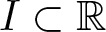$I\subset \mathbb{R}$ and function $u: I\to \mathbb{R}$, we define $Z_I[(u)]$ as the number of zero points of u on I. We show the following.

Corollary 2.3. Suppose (H3). Let $\{(\lambda_n,\mu_n,u_n)\}$ be a sequence of solutions of (1.3) with $\mu_n\to \infty$ and there exists a number $ \lambda_*\in[0,\infty)$ such that $\lambda_n\to \lambda_*$ as $n\to \infty$. Assume U(r) is a continuous function defined for all small r > 0. Furthermore, we suppose (i) or (ii) below.

1. (i) $\lambda_*\not=0$ and for any $\varepsilon\in(0,2)$ and $L\in \mathbb{R}$, there exists a constant $r_0\in(0,1)$ such that

   \begin{equation*} U_{2-\varepsilon}(r)\le U(r)\le V_L(r) \end{equation*}

   for all $r\in(0,r_0)$.

2. (ii) $\lambda_*=0$ and for any $\varepsilon \gt 0$, there exist values $r_0\in(0,1)$ and $L\in \mathbb{R}$ such that

   \begin{equation*} U_{2-\varepsilon}(r)\le U(r)\le V_L(r) \end{equation*}

   for all $r\in(0,r_0)$.

Then, up to a subsequence, for any $k\in \mathbb{N}\cup\{0\}$, there exist sequences $(r_{k,n}^{\pm})\subset (0,1)$ such that $u_n(r_{k,n}^{\pm})/\mu_n\to \delta_k$ as $n\to \infty$, $r_{k,n}^- \lt r_{k,n} \lt r_{k,n}^+$, and $u_n(r_{k,n}^\pm)=U(r_{k,n}^\pm)$ for all large $n \in\mathbb{N}$. In particular, for any sequence $(r_n)\subset (0,1)$ with $u_n(r_n)/\mu_n\to0$ as $n\to \infty$, it holds that

\begin{equation*} \lim_{n\to \infty}Z_{(0,r_n)}[u_n-U]=\infty. \end{equation*}

Notice that, in this result, we give not only estimates for intersection numbers but also precise information on positions where intersections occur. In particular, we find that two intersection points $r_{k,n}^{\pm}$ appear around the centre $r_{k,n}$ of $(k+1)$th bubble for all $k\in \mathbb{N}\cup\{0\}$. Since k is arbitrary, we ensure the divergence of the intersection numbers. For example, suppose $f(t)=e^{t^p}$ for all large t > 0 with p > 2. Then, for any $\theta \gt 1-1/p$, if we choose a continuous function U(r) so that

\begin{equation*} U(r)=\left\{2\log{\frac1r}-\theta \log{\left(2\log{\frac1{r}}\right)}+o\left(\log{\left(2\log{\frac1{r}}\right)}\right)\right\}^{\frac1p} \end{equation*}

as $r\to 0^+$, then the previous theorem proves that

\begin{equation*} \lim_{n\to \infty}Z_{(0,1)}[u_n-U]=\infty. \end{equation*}

Finally, for the next application, we give a similar intersection result for any sequence $\{(\bar{r}_n,\bar{\mu}_n,\bar{u}_n)\}$ which solves the next problem,

(2.6)\begin{equation} \begin{cases} -\bar{u}_n''-\frac1r\bar{u}_n'=f(\bar{u}_n),\ \bar{u}_n \gt 0\,\,\text{in }(0,\bar{r}_n),\\ \bar{u}_n(0)=\bar{\mu}_n,\ \bar{u}_n'(0)=0=\bar{u}_n(\bar{r}_n). \end{cases} \end{equation}

We get the following.

Corollary 2.4. Assume (H3). Let $\{(\bar{r}_n,\bar{\mu}_n,\bar{u}_n)\}$ be a sequence of solutions of (2.6) with $\bar{\mu}_n\to \infty$ as $n\to \infty$. Moreover, suppose that $\bar{U}(r)$ is a continuous function defined for all small r > 0 and that for any values $\varepsilon\in (0,2)$ and $L\in \mathbb{R}$, there exists a constant $r_0\in(0,1)$ such that

\begin{equation*} U_{2-\varepsilon}(r)\le \bar{U}(r)\le V_L(r) \end{equation*}

for all $r\in(0,r_0)$. Then for any sequence $(r_n)\subset (0,\bar{r}_n]$ such that $\bar{\mu}_n^{-p}\log{(1/r_n)}\to0$ as $n\to \infty$, we have that

\begin{equation*} \lim_{n\to \infty}Z_{(0,r_n)}[\bar{u}_n-\bar{U}]=\infty \end{equation*}

up to a subsequence.

We apply this result to prove the infinite oscillation of the bifurcation diagram of (1.2).

2.3. Oscillations of bifurcation diagrams

Lastly, we shall demonstrate how our oscillation estimates work for getting the infinite oscillation of the bifurcation diagram of (1.2). To this end, we consider the condition, inspired by Lemma 5.2 in [Reference Ghergu, Giacomoni and Prashanth6] and Proposition 2.1 in [Reference Ioku, Ruf and Terraneo8],

1. (H4) p > 2, $f\in C^2([0,\infty))$, and there exists a value $\tau_0 \gt 0$ such that

   \begin{equation*} f(t)=\frac{4(p-1)}{p^2}t^{1-2p}e^{t^p} \end{equation*}

   for all $t\geqslant \tau_0$.

Notice that (H4) implies (H3). Moreover, we can obviously construct specific examples of f satisfying (H4). This assumption is reasonable for our aim since we can easily check the existence of a solution with a suitable singularity at the origin. See Lemma 3.11 below. Moreover, under (H4), we confirm that for any µ > 0, there exists a unique pair $(\lambda(\mu),u(\mu,\cdot))$ of a number and a function in $C^{2,\alpha}([0,1])$ such that $(\lambda,u)=(\lambda(\mu),u(\mu,\cdot))$ solves (1.2) and $u(\mu,0)=\mu$. For the proof, see Theorem 3 in [Reference Atkinson and Peletier2] or Lemma 2.1 in [Reference Adimurthi and Giacomoni1] with Theorem 2.1 in [Reference Nabana and de Thélin16] and the standard regularity theory. Then, combining this fact with Theorem 2.1 in [Reference Korman10], one sees that the map $\mu \mapsto (\lambda(\mu),u(\mu,\cdot))$ draws a C ¹ curve in $\mathbb{R}\times C^{2,\alpha}([0,1])$. Let us show the oscillation behaviour of this solution’s curve as $\mu\to \infty$.

For this purpose, for each µ > 0, we set $\bar{u}(\mu,r)=u(\mu,r/\sqrt{\lambda})$ for all $r\in[0,\sqrt{\lambda}]$. Then $\bar{u}=\bar{u}(\mu,\cdot)$ satisfies

(2.7)\begin{equation} \begin{cases} -\bar{u}''-\frac1r\bar{u}'=f(\bar{u}),\ \bar{u} \gt 0 \ \text{in }(0,\bar{r}),\\ \bar{u}(0)=\bar{\mu},\ \bar{u}'(0)=0=\bar{u}(\bar{r}), \end{cases} \end{equation}

with $\bar{r}=\sqrt{\lambda}$ and $\bar{\mu}=\mu$. Furthermore, for any $\bar{R} \gt 0$, we consider the next probelm,

(2.8)\begin{equation} \begin{cases} -\bar{U}''-\frac1r \bar{U}'=f(\bar{U}),\ \bar{U} \gt 0 \ \text{in }(0,\bar{R}),\\ \lim_{r\to 0^+}\bar{U}(r)=\infty,\ \bar{U}(\bar{R})=0. \end{cases} \end{equation}

Under (H4), we will prove in Lemma 3.11 that there exists a pair of a value $\bar{R}^*$ and a smooth function $\bar{U}^*$on $(0,1]$ such that $\bar{U}^*(r)=(2\log{(1/r)})^{1/p}$ for all small r > 0 and $(\bar{R},\bar{U})=(\bar{R}^*,\bar{U}^*)$ satisfies (2.8). Note also that if we put $\lambda^*=(\bar{R}^*)^2$ and $U^*(r)=\bar{U}^*(\sqrt{\lambda^*}r)$ for all $r\in(0,1]$, $(\lambda,U)=(\lambda^*,U^*)$ solves the next problem,

(2.9)\begin{equation} \begin{cases} -{U}''-\frac1r {U}'=\lambda f({U}),\ U \gt 0 \ \text{in }(0,1),\\ \lim_{r\to 0^+}{U}(r)=\infty,\ {U}(1)=0. \end{cases} \end{equation}

Corollary 2.4 succeeds in proving that the intersection number between any solution $\bar{u}$ of (2.7) and $\bar{U}^*$ diverges to infinity as $\bar{\mu}\to \infty$. Then we may apply the argument in [Reference Miyamoto13] and get the desired result as follows.

As stated here, our oscillation estimates successfully allow us to prove the infinite oscillation of the bifurcation diagram. Surely, it will enable us to find more nonlinearities f which yield the infinite oscillation of the bifurcation diagram of (1.2) once the existence and the asymptotic behaviour of the solutions of (2.8) are confirmed. Fortunately, this is done for the general nonlinearity by [Reference Fujishima, Ioku, Ruf and Terraneo5] very recently. Thanks to this, we can confirm that the same oscillation results hold true for the standard examples of f. See Remark 2.6 below. Finally, we remark that, we do not prove that $(\lambda(\mu),u(\mu,\cdot))\to (\lambda^*,U^*)$ as $\mu\to \infty$ since the proof seems to require more arguments and to be beyond the main aim of this series of papers. Hence, we leave them open here as an interesting question for the future. (Very recently, the convergence of blow-up solutions to a singular solution is discussed in [Reference Kumagai11].) Let us finally remark on a fruitful consequence of the interaction between the existence result in [Reference Fujishima, Ioku, Ruf and Terraneo5] and our oscillation estimates.

The next section is devoted to the proof of our main results.

3.1. Preliminaries

We first recall some basic facts that will be used for our proof. We begin with two basic properties of our nonlinearity. First, (H1) implies the next one.

Lemma 3.1. Suppose (H1). Then it holds that

(3.1)\begin{equation} \lim_{t\to \infty}\frac{\log {h(t)}}{t^p}=0. \end{equation}

The proof is given by Lemma 2.1 in [Reference Naimen17]. The next one is a consequence of (H2).

Lemma 3.2. Assume (H2). Then

\begin{equation*} \sup\{\lambda \gt 0\ |\ \text{(1.1) has a classical solution $u$} \} \lt \infty. \end{equation*}

For the proof, see Lemma 2.4 in [Reference Naimen17]. We next give an identity, which was a key tool for our previous concentration analysis. Let $\{(\lambda_n,\mu_n,u_n)\}$ be a sequence of solutions of (1.3).

Lemma 3.3. Let $0 \lt s \lt t\le1$. Then, we get that

(3.2)\begin{equation} u_n(s)-u_n(t)=\left(\log{\frac{t}{s}}\right)\int_{0}^{s} \lambda_nf(u_n(r))rdr+\int_{s}^{t} \lambda_nf(u_n(r))r\log{\frac{t}{r}}dr. \end{equation}

The proof is done by Lemma 2.5 in [Reference Naimen17]. This is still a key identity in this paper to connect our concentration and oscillation estimates. Lastly we recall some properties of sequences $(a_k)$ and $(\delta_k)$ defined by (1.7) and (1.8).

Lemma 3.5. Suppose p > 2. For any $k\in \mathbb{N}\cup\{0\}$, put $E_k=2a_k/\delta_k^{p-1}$. Then we have that

\begin{equation*} \delta_k^{p-1}\sum_{i=0}^kE_i=2+a_k. \end{equation*}

For the proofs of these two lemmas, see Lemmas 4.16, 4.18, and 2.13 in [Reference Naimen17].

3.2. Proofs of Theorem 2.1 and its corollaries

Let us start the proof of Theorem 2.1. Assume $\{(\lambda_n,\mu_n,u_n)\}$ is a sequence of solutions of (1.3) such that $\mu_n\to \infty$ as $n\to \infty$. The next Lemma proves (2.1).

Lemma 3.6. Assume $(\rho_{0,n})$ is a sequence obtained in Theorem 1.1 and take any sequences $(r_n)\subset (0,\rho_{0,n}]$ and $(R_n)\subset (0,\infty)$ such that $r_n=R_n \gamma_{0,n}$ for all $n\in \mathbb{N}$. Then we have that

\begin{equation*} p \lambda_n r_n^2u_n(r_n)^{p-1}f(u_n(r_n))=\frac{64R_n^2}{(8+R_n^2)^2}(1+o(1)) \end{equation*}

as $n\to \infty$.

Proof. The proof is given in Lemma 3.3 in [Reference Naimen17]. For the readers’ convenience, we show the proof. Using Theorem 1.1 (see also Lemma 3.2 in [Reference Naimen17]), we get that

\begin{equation*} \begin{split} p \lambda_nr_n^2 u_n(r_n)^{p-1}f(u_n(r_n))&=\left(\frac{u_n(r_n)}{\mu_n}\right)^{p-1}\left(\frac{r_n}{\gamma_{0,n}}\right)^2\frac{f(u_n(r_n))}{f(\mu_n)}\\ &=(1+o(1))R_n^2e^{z_0(R_n)+o(1)}\\ \end{split} \end{equation*}

as $n\to \infty$. This completes the proof.

We next show (2.4).

Lemma 3.7. Assume p > 2, (H1), and $k\in \mathbb{N}$. Let $(r_n)\subset [\bar{\rho}_{k,n},\rho_{k,n}]$ and $(R_n)\subset (0,\infty)$ be sequences of values such that $r_n=R_n \gamma_{k,n}$ for all $n\in \mathbb{N}$. Then we get that

\begin{equation*} p\lambda_nr_n^2 u_n(r_n)^{p-1}f(u_n(r_n)) =\frac{2a_k^2 b_k R_n^{a_k}}{(1+b_k R_n^{a_k})^2}(1+o(1)) \end{equation*}

as $n\to \infty$.

Proof. Put $u_n(r_{k,n})=\mu_{k,n}$ for all $n\in \mathbb{N}$. Using the results in Theorem 1.2 (see also Lemma 4.12 in [Reference Naimen17]), we compute similarly to the previous proof that

\begin{equation*} \begin{split} p \lambda_nr_n^2 u_n(r_n)^{p-1}f(u_n(r_n))&=\left(\frac{u_n(r_n)}{\mu_{k,n}}\right)^{p-1}\left(\frac{r_n}{\gamma_{k,n}}\right)^2\frac{f(u_n(r_n))}{f(\mu_{k,n})} \\ &=(1+o(1))R_n^2e^{z_k(R_n)+o(1)} \end{split} \end{equation*}

as $n\to \infty$. This proves the lemma.

In the following, we note the next consequence of Theorems 1.1 and 1.2.

Lemma 3.8. Suppose (H1) with p > 2 and $k\in \mathbb{N}$. Put $\mu_{0,n}=\mu_n$ if k = 0 and $\mu_{k,n}=u_n(r_{k,n})$ if $k\not=0$ for all $n\in \mathbb{N}$. Then, we have that

\begin{equation*} \lim_{n\to \infty}\frac{\log{(\rho_{k,n}/r_{k,n})}}{\mu_{k,n}^{p}}=0= \lim_{n\to \infty}\frac{\log{(\bar{\rho}_{k,n}/r_{k,n})}}{\mu_{k,n}^{p}} \end{equation*}

where we assumed $k\not=0$ for the latter equality.

Proof. We have from Theorems 1.1 and 1.2 that

\begin{equation*} 1+o(1)=\frac{u_n(\rho_{k,n})}{\mu_{k,n}}=1+\frac{z_k(\rho_{k,n}/\gamma_{k,n})+o(1)}{p\mu_{k,n}^p} \end{equation*}

as $n\to \infty$. Since $(r_{k,n}/\gamma_{k,n})^2=a_k^2/2+o(1)$ as $n\to \infty$, we get the first equality. The second one is similarly proved. We finish the proof.

We finally confirm (2.3).

Lemma 3.9. Assume p > 2, (H1), and $k\in \mathbb{N}\cup\{0\}$. Then for any sequence $(r_n)\subset [\rho_{k,n},\bar{\rho}_{k+1,n}]$ and value $\delta\in [\delta_{k+1},\delta_k]$ such that $u_n(r_n)/\mu_n\to \delta$ as $n\to \infty$, we obtain

\begin{equation*} u_n(r_n)=\left\{(\beta_k(\delta)+o(1))\log{\frac1{r_n}}\right\}^{\frac1p} \end{equation*}

as $n\to \infty$.

Proof. From (3.2), we get

\begin{equation*} u_n(\rho_{k,n})-u_n(r_n)\geqslant\left(\log{\frac{r_n}{\rho_{k,n}}}\right)\int_{0}^{\rho_{k,n}} \lambda_nf(u_n(r))rdr, \end{equation*}

and also

\begin{equation*} u_n(\rho_{k,n})-u_n(r_n) \le \left(\log{\frac{r_n}{\rho_{k,n}}}\right)\int_{0}^{\bar{\rho}_{k+1,n}} \lambda_nf(u_n(r))rdr. \end{equation*}

Hence, using the first assertion in (1.10), we have

\begin{equation*} \begin{split} p\mu_n^{p-1}&\left( u_n(\rho_{k,n})-u_n(r_n)\right)\\ &=\left(\log{\frac{1}{\rho_{k,n}}}-\log{\frac{1}{r_n}}\right)\left(p\mu_n^{p-1}\int_0^{\rho_{k,n}} \lambda_nf(u_n)rdr+o(1)\right). \end{split} \end{equation*}

Then, noting (1.14), (1.10), Lemmas 3.8 and 3.5, we get

\begin{equation*} \frac{\log{\frac{1}{\rho_{k,n}}}}{\mu_n^p}=\frac{\log{\frac{1}{r_{k,n}}}+\log{\frac{r_{k,n}}{\rho_{k,n}}}}{\mu_n^p}=\frac{\delta_k^p}{2}+o(1)\end{equation*}

and

\begin{equation*} p\mu_n^{p-1}\int_0^{\rho_{k,n}} \lambda_nf(u_n)rdr= \frac{2+a_k}{\delta_k^{p-1}}+o(1) \end{equation*}

as $n\to \infty$. Applying these facts and our assumption $\mu_n=(\delta^{-1}+o(1))u_n(r_n)$ for the previous formula, we calculate

\begin{equation*} \begin{split} p\left(\frac{\delta_k }{\delta}\right)^p&\left(1-\frac{\delta}{\delta_k}+o(1)\right)u_n(r_n)^p\\ &=\left\{\frac{1+o(1)}{2}\left(\frac{\delta_k}{\delta}\right)^pu_n(r_n)^p-\log{\frac{1}{r_n}}\right\}(2+a_k+o(1)). \end{split} \end{equation*}

Solving this formula with respect to $u_n(r_n)$, we get the conclusion. This finishes the proof.

Let us show Theorem 2.1

Next, we prove the corollaries. In the following proofs, we recall the constants $\delta_k^*$ and $\beta_k^*$ for all $k\in \mathbb{N}\cup\{0\}$ defined below Theorem 2.1. To prove Corollary 2.3, we give the next lemma.

Lemma 3.10. Assume p > 2, (H3), and $k\in \mathbb{N}\cup\{0\}$. Then we get

\begin{equation*} \begin{split} u_n(r_{k,n})=\left\{2\log{\frac1{r_{k,n}}}-\left(1-\frac{1-m}{p}\right) \log{\left(2\log{\frac1{r_{k,n}}}\right)}+\log{\frac{a_k^2}{2c_0p \lambda_n}}+o(1)\right\}^{\frac1p} \end{split} \end{equation*}

as $n\to \infty$.

Proof. The conclusion readily follows from (1.6) with (2.2) if k = 0 and (1.9) with (2.5) if $k\in \mathbb{N}$.

Let us complete the proof.

Proof of Corollary 2.3

Assume $k\in \mathbb{N}\cup\{0\}$. Choose a sequence $(r_{k,n}^*)\subset (\rho_{k,n},\bar{\rho}_{k+1,n})$ such that $u_n(r_{k,n}^*)/\mu_n\to \delta_k^*$ as $n\to \infty$. In addition, if $k\not=0$, select a sequence $(r_{k-1,n}^*)\subset (\rho_{k-1,n},\bar{\rho}_{k,n})$ so that $u_n(r_{k-1,n}^*)/\mu_n\to \delta_{k-1}^*$ as $n\to \infty$. Then fix a number $\beta\in(\beta_k^*,2)$. Moreover, in the case of (i), we choose any number $L \lt \log{(a_k^2/(2c_0p\lambda_*)}$. Then we have by the assumption that $U_\beta(r)\le U(r)\le V_L(r)$ for all small r > 0. On the other hand, in the case of (ii), noting the assumption, we select any value L > 0 and get $U_\beta(r)\le U(r)\le V_L(r)$ for all small r > 0. Then, in each case, we get from Lemma 3.10 and (2.3) that $U(r_{k,n})\le V_L(r_{k,n}) \lt u_n(r_{k,n})$ and $U(r_{k,n}^*)\geqslant U_{\beta}(r_{k,n}^*) \gt u_n(r_{k,n}^*)$ for all large $n\in \mathbb{N}$. Furthermore, if $k\geqslant1$, since $\beta_{k-1}^* \lt \beta_k^*$, we have that $U(r_{k-1,n}^*)\geqslant U_\beta (r_{k-1,n}^*) \gt u_n(r_{k-1,n}^*)$ for all large $n\in \mathbb{N}$. Consequently, we obtain sequences $(r_{k,n}^{\pm})\subset (0,1)$ such that $r_{k-1,n}^* \lt r_{k,n}^- \lt r_{k,n} \lt r_{k,n}^+ \lt r_{k,n}^*$, where we regard $r_{k-1,n}^*=0$ when k = 0, and $u_n(r_{k,n}^{\pm})=U(r_{k,n}^{\pm})$ for all large $n\in \mathbb{N}$. Furthermore, we have that $u_n(r_{k,n}^\pm)/\mu_n\to \delta_k$ as $n\to \infty$ by (2.3). This proves the former conclusion. Finally, take any sequence $(r_n)\subset (0,1)$ such that $u_n(r_n)/\mu_n\to0$ as $n\to \infty$. Then the former assertion implies that for any $k\in \mathbb{N}\cup\{0\}$, we get that $r_{k,n}^+ \gt r_n$ for all large $n\in \mathbb{N}$ and thus,

\begin{equation*} Z_{(0,r_n)}[u_n-U]\geqslant 2(k+1) \end{equation*}

for all large $n\in \mathbb{N}$. Since k is arbitrary, we finish the proof.

Lastly, we prove Corollary 2.4.

Proof of Corollary 2.4

Put $u_n(r)=\bar{u}_n(\bar{r}_nr)$ for all $r\in[0,1]$, $\lambda_n=\bar{r}_n^2$, and $\mu_n=\bar{\mu}_n$ for all $n\in \mathbb{N}$. Then $\{(\lambda_n,\mu_n,u_n)\}$ is a sequence of solutions of (1.3). It follows from Theorems 1.1, 1.2, and (2.3) that, for any $k\in \mathbb{N}\cup \{0\}$, there exist sequences $(r_{k,n}),(r_{k,n}^*)\subset (0,1)$ such that $u_n(r_{k,n})/\mu_n\to \delta_k$, $u_n(r_{k,n}^*)/\mu_n\to \delta_k^*$,

\begin{equation*} p\lambda_nr_{k,n}^2 u_n(r_{k,n})^{p-1}f(u_n(r_{k,n}))= \frac{a_k^2}{2}+o(1), \end{equation*}

and

\begin{equation*} u_n(r_{k,n}^*)=\left\{(\beta_k^*+o(1))\log{\frac1{r_{k,n}^*}}\right\}^{\frac1p} \end{equation*}

as $n\to \infty$. Putting $\bar{r}_{k,n}=\sqrt{\lambda_n}r_{k,n}$ and $\bar{r}_{k,n}^*=\sqrt{\lambda_n}r_{k,n}^*$ for all $n\in \mathbb{N}$, these two formulas imply

(3.3)\begin{equation} p\bar{r}_{k,n}^2 \bar{u}_n(\bar{r}_{k,n})^{p-1}f(\bar{u}_n(\bar{r}_{k,n}))=\frac{a_k^2}{2}+o(1) \end{equation}

and

(3.4)\begin{equation} \bar{u}_n(\bar{r}_{k,n}^*)=\left\{(\beta_k^*+o(1))\log{\frac{1}{\bar{r}_{k,n}^*}}\right\}^{\frac1p} \end{equation}

where we used (1.13), (1.14), and the fact that $r_{k,n} \lt r_{k,n}^* \lt r_{k+1,n}$ for all large $n\in \mathbb{N}$. Furthermore, similarly to the proof of Lemma 3.10, we deduce from (3.3) that

(3.5)\begin{equation} \begin{split} &\bar{u}_n(\bar{r}_{k,n}) =\left\{2 \log{\frac1{\bar{r}_{k,n}}} -\left(1-\frac{1-m}{p}\right) \log{\left(2\log{\frac1{\bar{r}_{k,n}}}\right)}+\log{\frac{a_k^2}{2c_0p }}+o(1)\right\}^{\frac1p}. \end{split} \end{equation}

Then by (3.4), (3.5), and our assumption, we get $\bar{U}(\bar{r}_{k,n}) \lt \bar{u}_n(\bar{r}_{k,n})$ and $\bar{u}_n(\bar{r}_{k,n}^*) \lt \bar{U}(\bar{r}_{k,n}^*)$ for all large $n\in \mathbb{N}$. Hence, there exists a sequence $(\bar{s}_{k,n})\subset(\bar{r}_{k,n},\bar{r}_{k,n}^*)$ such that $\bar{u}_n(\bar{s}_{k,n})=\bar{U}(\bar{s}_{k,n})$ for all large $n\in \mathbb{N}$. Finally, choose any sequence $(r_n)\subset (0,1)$ so that $\bar{\mu}_n^{-p}\log{(1/r_n)}\to 0$ as $n\to \infty$. Then, we have that $\log{(1/r_n)}/\log{(1/\bar{s}_{k,n})} \to0$ as $n\to \infty$ by (1.13) and (1.14). In particular, $\bar{s}_{k,n} \lt r_n$ for all large $n\in \mathbb{N}$. This implies that $Z_{(0,r_n)}[\bar{u}_n-\bar{U}]\geqslant k+1$ for all large $n\in \mathbb{N}$. Since k is arbitrary, we get $Z_{(0,r_n)}[\bar{u}_n-\bar{U}]\to \infty$ as $n\to \infty$. This finishes the proof.

3.3. Proof of Theorem 2.5

Finally, we shall show Theorem 2.5. To this end, we first prove the existence of a solution of (2.8).

Proof. We refer to the idea in the proof of Proposition 2.1 in [Reference Ioku, Ruf and Terraneo8] and Lemma 2.1 in [Reference Adimurthi and Giacomoni1]. Set $R_0=e^{-\tau_0^p/2}$. First it is easy to check that $-\{(2\log{(1/r)})^{1/p}\}''-\{(2\log{(1/r)})^{1/p}\}'/r=f((2\log{(1/r)})^{1/p})$ and $(2\log{(1/r)})^{1/p} \gt 0$ for all $r\in(0,R_0]$. Next we solve the initial value problem,

(3.6)\begin{equation} \begin{cases} -\bar{U}''-\frac1r \bar{U}'=f(\bar{U}) \ \text{in }(0,\infty),\\ \bar{U}(R_0)=\tau_0, \bar{U}'(R_0)=-2/(p\tau_0^{p-1}R_0). \end{cases} \end{equation}

By (H4), there exists a value $\varepsilon \gt 0$ such that (3.6) admits a unique solution $\bar{U}$ on $(0,R_0+\varepsilon)$ and $\bar{U}(r)=(2\log{(1/r)})^{1/p}$ for all $r\in (0,R_0]$. Define the value

\begin{equation*} \begin{split} R^*:=\sup\{r \gt R_0\ |\ &\text{the solution}\,\, \bar{U}(s)\,\, \text{of}\,\, (3.6)\ \text{exists and}\,\, \bar{U}(s) \gt 0 \\ &\ \ \ \ \ \ \ \ \ \ \ \ \ \ \ \ \ \ \ \ \ \ \ \ \ \ \ \ \ \ \ \ \ \ \ \ \ \ \ \ \ \ \text{for all}\,\, s\in (0,r)\}. \end{split} \end{equation*}

Then, for any $r\in(R_0,R^*)$, integrating the equation gives

\begin{equation*} -r\bar{U}'(r)=-R_0\bar{U}'(R_0)+\int_{R_0}^{r}f(\bar{U})rdr \gt 0 \end{equation*}

by the initial condition and (H0). In particular, $\bar{U}(r)$ is strictly decreasing on $(0,R^*)$. Moreover, we have that $R^* \lt \infty$. If not, $\bar{U} \gt 0$ on $(0,\infty)$. Then, for any $r\in(R_0+1,\infty)$, integrating the equation, we get that

\begin{equation*} -\bar{U}'(r) \geqslant\left(-R_0\bar{U}'(R_0)+\int_{R_0}^{R_0+1}f(\bar{U})sds\right)\frac1r \end{equation*}

by (H0). For any $r\in(R_0+1,\infty)$, integrating again gives

\begin{equation*} 0 \lt \bar{U}(r)\le\bar{U}(R_0+1)-\left(-R_0\bar{U}'(R_0)+\int_{R_0}^{R_0+1}f(\bar{U})sds\right)\log{\frac{r}{R_0+1}}. \end{equation*}

Since the right-hand side diverges to $-\infty$ as $r\to \infty$, we get a contradiction. Then noting the monotonicity, we obtain $\lim_{r\to R^{*-}}\bar{U}(r)=0$. Therefore, setting $\bar{R}^*=R^*$ and $\bar{U}^*=\bar{U}$ on $(0,\bar{R}^*)$ with $\bar{U}^*(\bar{R}^*)=0$, we get the desired solution. This finishes the proof.

Now, we can show the oscillation of the bifurcation diagram by combining our intersection estimates and the idea in the proof of Lemma 3.5 in [Reference Miyamoto13]. (We also refer the readers to the proof of Lemma 5 in [Reference Miyamoto14].)

Proof. For every µ > 0, put $r(\mu)=\sqrt{\lambda(\mu)}$ and $\bar{u}(\mu,r)=u(\mu,r/\sqrt{\lambda(\mu)})$ for all $r\in[0,r(\mu)]$. Note that from our assumption, $r(\mu)$ and $\bar{u}(\mu,r)$ are C ¹ functions with respect to each variable. Moreover, let $(\lambda^*,U^*)$ be the pair of the number and function in the assumption of Theorem 2.5. Set $r^*=\sqrt{\lambda^*}$ and $\bar{U}^*(r)=U^*(r/\sqrt{\lambda^*})$ for all $r\in (0,r^*]$. Then for any µ > 0, $\bar{u}=\bar{u}(\mu,\cdot),\bar{U}^*$ are solutions of the equation,

(3.7)\begin{equation} -\bar{u}''-\frac1r \bar{u}'=f(\bar{u}) \ \text{in }(0,\min\{r(\mu),r^*\}). \end{equation}

Put $v(\mu,r)=\bar{U}^*(r)-\bar{u}(\mu,r)$ for all µ > 0 and $r\in(0,\min\{r(\mu),r^*\}]$. Then, $v(\mu,r)$ is a C ¹ function with respect to each variable. It also holds that, for each µ > 0,

(3.8)\begin{equation} \lim_{r\to 0^+}v(\mu,r)=\infty. \end{equation}

Moreover, we obtain that

(3.9)\begin{equation} \lim_{\mu\to \infty}Z_{(0,\min\{r(\mu),r^*\}]}[v(\mu,\cdot)]=\infty. \end{equation}

If not, there exists a sequence $(\mu_n)\subset (0,\infty)$ such that $\mu_n\to \infty$ as $n\to \infty$ and

\begin{equation*} \sup_{n\in \mathbb{N}}Z_{(0,\min\{r(\mu_n),r^*\}]}[v(\mu_n,\cdot)] \lt \infty. \end{equation*}

Then noting $\mu_n^{-p}\log{(\min\{r(\mu_n),r^*\})}\to 0$ as $n\to \infty$ by (1.13), we get a contradiction with Corollary 2.4. This proves (3.9). On the other hand, we claim that for each µ > 0,

(3.10)\begin{equation} Z_{(0,\min\{r(\mu),r^*\}]}[v(\mu,\cdot)] \ \text{is finite}. \end{equation}

If this is not true, for some µ > 0, noting (3.8), we find a value $r_0\in(0,\min\{r(\mu),r^*\}]$ and a sequence $(r_n)\subset (0,\min\{r(\mu),r^*\}]$ such that $r_n\not=r_0$ and $v(r_n)=0$ for all $n\in \mathbb{N}$ and $r_n\to r_0$ as $n\to \infty$. It follows that $v(\mu,r_0)=0$ and $v_r(\mu,r_0)=0$ where v_r denotes the partial derivative of v with respect to r. This contradicts the uniqueness of solutions of the initial value problem of (3.7). This proves the claim.

Now the uniqueness of (3.7) again and the implicit function theorem imply that any zero point of $v(\mu,\cdot)$ on $(0,\min\{r(\mu),r^*\}]$ continuously depends on µ and further, as µ increases or decreases, it does not split into two or more zero points or collide with any other one. Hence, noting also (3.8), we have that any change of the number of zero points on $(0,\min\{r(\mu),r^*\}]$ occurs only at the boundary $\min\{r(\mu),r^*\}$ and only when $r(\mu)$ leaves or touches $r^*$. Then, we can prove that $r(\mu)$ oscillates around $\lambda^*$ infinitely many times. To see this, we first show that there exists a sequence $(\mu_n)\subset (0,\infty)$ such that $\mu_n\to \infty$ and $r(\mu_n)=r^*$ for all $n\in \mathbb{N}$. If the assertion fails, then there exists a value $\mu_0 \gt 0$ such that $r(\mu)\not= r^*$ for all $\mu\geqslant \mu_0$. Then the previous conclusion and (3.10) yield that $Z_{(0,\min\{r(\mu),r^*\}]}[v(\mu,\cdot)]=Z_{(0,\min\{r(\mu_0),r^*\}]}[v(\mu_0,\cdot)] \lt \infty$ for all $\mu\geqslant \mu_0$. This contradicts with (3.9). On the other hand, we can similarly prove that there exists a sequence $(\mu_n')\subset (0,\infty)$ such that $\mu_n'\to \infty$ and $r(\mu_n')\not=r^*$ for all $n\in \mathbb{N}$.

Consequently, recalling that $\lambda(\mu)=r(\mu)^2$ and $\lambda^*=(r^*)^2$, we prove the desired conclusion of the lemma. We finish the proof.

We shall show Theorem 2.5

We end this section by giving the proof for the discussion in Remark 2.6.

Remark 3.13. Finally, let us check the intersection properties for the two examples in Remark 2.6. First assume f satisfies $f(t)=t^m e^{t^p}$ for all large t > 0 with $m\in \mathbb{R}$ and p > 2 and some suitable conditions. In this case, by [Reference Fujishima, Ioku, Ruf and Terraneo5], we confirm that (2.8) admits a solution $\bar{U}$ such that

\begin{equation*} \begin{split} \bar{U}(r)=&\left\{2\log{\frac1r}-\left(2-\frac{1-m}{p}\right)\log{\left(2\log{\frac1{r}}\right)}+\log{\frac{4(p-1)}{p^2}}\right\}^{\frac1p}\\ &+O\left(\frac{\log{\left(\log{\frac1r}\right)}}{\left(\log{\frac1r}\right)^{2-1/p}}\right) \end{split} \end{equation*}

as $r\to0^+$. See Theorems 2.1, 2.2, and Example 4.1 there. Hence, by Corollary 2.4, the intersection numbers between blow-up solutions of (2.6) and $\bar{U}$ diverge to infinity. This allows us to obtain the same conclusion with (3.9) in the proof of Lemma 3.12 and thus, we complete the desired oscillation assertions. Next suppose f verifies $f(t)=e^{t^p+t^q}$ for all large t > 0 with p > 2 and $0 \lt 2q \lt p$ and some appropriate assumptions. Put

\begin{equation*} w(r)=\frac{p'}{4}r^2\left(\log{\frac1{r^2}}+1\right) \end{equation*}

where $1/p+1/p'=1$. Then from [Reference Fujishima, Ioku, Ruf and Terraneo5], we ensure the existence of solutions $\bar{U}$ of (2.8) such that

\begin{equation*} \begin{split} \bar{U}(r)&=\left\{-\log{w}-(-\log{w})^{\frac qp}-\left(1-\frac{1}{p}\right)\log{(-\log{w})}+\log{\frac1p}\right\}^{\frac1p}\\ &+O\left(\frac{1}{\left(-\log{w}\right)^{2-1/p-2q/p}}\right) \end{split} \end{equation*}

as $r\to 0^+$. Check Example 4.2 there. It follows that

(3.11)\begin{equation} \begin{split} \bar{U}&(r)^p+\bar{U}(r)^q= 2\log{\frac1r}-\left(2-\frac{1}{p}\right)\log{\left(2\log{\frac1r}\right)}+O(1) \end{split} \end{equation}

as $r\to0^+$. On the other hand, let $\{(\bar{r}_n,\bar{\mu}_n,\bar{u}_n)\}$ be any sequence of solutions of (2.6) such that $\bar{\mu}_n\to \infty$ as $n\to \infty$. Then similarly to the proof of (3.5), for each $k\in \mathbb{N}\cup\{0\}$, we find a sequence $(\bar{r}_{k,n})$ such that $\bar{r}_{k,n}\to0$ and

(3.12)\begin{equation} \begin{split} &\bar{u}_n(\bar{r}_{k,n})^p+\bar{u}_n(\bar{r}_{k,n})^q=2 \log{\frac1{\bar{r}_{k,n}}} -\left(1-\frac{1}{p}\right) \log{\left(2\log{\frac1{\bar{r}_{k,n}}}\right)}+O(1) \end{split} \end{equation}

as $n\to \infty$. In particular, $\bar{U}(\bar{r}_{k,n}) \lt \bar{u}_{k,n}(\bar{r}_{k,n})$ for all large $n\in \mathbb{N}$. Hence, using (3.11) and (3.12), similarly to Corollary 2.4, we get that the intersection number between $\bar{u}_n$ and $\bar{U}$ diverges to infinity as $n\to \infty$. Then, analogously to the former case, we arrive at the desired oscillation result. We finish the proof.

4.1. Infinite sequence of bubbles in the limit cases

We begin by discussing what happens on the infinite sequence $(z_k)$ of the limit profiles, obtained in Theorem 1.2, in the limits $p\to 2^+$ and $\infty$. To do this, we recall the sequences $(\delta_k)$ and $(a_k)$ of numbers defined by (1.7) and (1.8) and $(\beta_k^*)$ below Theorem 2.1. For each $k\in \mathbb{N}\cup\{0\}$, we write the dependence on p > 2 by $\delta_k=\delta_k(p)$, $a_k=a_k(p)$, $\beta_k^*=\beta_k^*(p)$, and $z_k=z_k^{(p)}$. First, we check the case $p\to2^+$. In this case, the singular limit profile turns into a regular one. We get the following.

Proposition 4.1. The case $p\to 2^+$

Assume p > 2. Then we have that for any $k\in \mathbb{N}$, $\delta_k(p)/\delta_{k-1}(p)\to0$ and $a_k(p)\to2$ as $p\to 2$. In particular, we get $\delta_k(p)\to0$ and $z_k^{(p)}(r)\to \tilde{z}_0(r)$ for any r > 0 as $p\to 2$ where

(4.1)\begin{equation} \tilde{z}_0(r)=\log{\frac{16}{(2+r^2)^2}} \end{equation}

which satisfies

\begin{equation*}\begin{cases} -\tilde{z}_0''-\frac1r \tilde{z}_0'=e^{\tilde{z}_0}\text{in }(0,\infty),\\ \tilde{z}_0(\sqrt{2})=0,\ \tilde{z}_0'(\sqrt{2})=-\sqrt{2}, \end{cases} \end{equation*}

and

\begin{equation*} \int_0^\infty e^{\tilde{z}_0}rdr=4. \end{equation*}

This is a reasonable observation in view of the classification result for the critical case p = 2 in [Reference Druet3] and [Reference Druet4], where all the concentrating parts are characterized by a regular limit profile. Especially, this shows a continuous connection between supercritical concentration phenomena and critical ones.

Next, we consider the case $p\to \infty$. In this case, interestingly, $z_k^{(p)}$ converges to another singular profile described by the Liouville equation with suitable limit formulas of (1.7) and (1.8). To see this, we put $\hat{a}_0=2$ and $\hat{c}_0=1$. Then, for all $k\in \mathbb{N}$, we define constants $\hat{a}_k\in(0,2)$ and $\hat{c}_k\in(0,\hat{c}_{k-1})$ by the relations,

(4.2)\begin{equation} \frac{2}{2+\hat{a}_{k-1}}\log{\frac{\hat{c}_{k-1}}{\hat{c}_k}}-1+\frac{\hat{c}_k}{\hat{c}_{k-1}}=0 \end{equation}

and

(4.3)\begin{equation} \hat{a}_k=2-\frac{\hat{c}_k}{\hat{c}_{k-1}}(2+\hat{a}_{k-1}). \end{equation}

These numbers are well-defined. See Lemma 4.4 below. Then we have the following.

Proposition 4.2 (The case $p\to \infty$)

Suppose p > 2. Then we get $\delta_k(p)^{p-1}\to \hat{c}_{k}$ and $a_{k}(p)\to \hat{a}_{k}$ as $p\to \infty$. Particularly, we obtain $\delta_k(p)\to1$ and $z_k^{(p)}(r)\to \hat{z}_k(r)$ for all r > 0 as $p\to \infty$ where $\hat{z}_k$ is defined by

(4.4)\begin{equation} \hat{z}_k(r)=\log{\frac{2\hat{a}_k^2 \hat{b}_k}{r^{2-\hat{a}_k}(1+\hat{b}_kr^{\hat{a}_k})^2}} \end{equation}

with $\hat{b}_k=(\sqrt{2}/\hat{a}_k)^{\hat{a}_k}$ and satisfies

\begin{equation*} \begin{cases} -\hat{z}_k''-\frac1r \hat{z}_k'=e^{\hat{z}_k}\text{in }(0,\infty),\\ \hat{z}_k(\hat{a}_k/\sqrt{2})=0,\ (\hat{a}_k/\sqrt{2})\hat{z}_k'(\hat{a}_k/\sqrt{2})=2, \end{cases} \end{equation*}

and

\begin{equation*} \int_0^\infty e^{\hat{z}_k}rdr=2\hat{a}_k. \end{equation*}

Moreover, we have that $\hat{a}_k$ is strictly decreasing with respect to $k\in \mathbb{N}$, $\hat{a}_k\to0$ as $k\to \infty$, and $\sum_{k=0}^\infty \hat{a}_k=\infty$. Especially, we deduce

\begin{equation*} \hat{z}_k(r)-\log{\frac{\hat{a}_k^2}{2}}\to 2\log{\frac1r} \end{equation*}

for any r > 0 as $k\to \infty$.

This observation leads us to expect that the limit recurrence formulas (4.2) and (4.3) play an important role in the analysis of supercritical problems with much stronger growth.

Now, let us remark on the infinite concentration and oscillation phenomena on sequences $\{(\lambda_n,\mu_n,v_n)\}$ of solutions of the next problem,

(4.5)\begin{equation} \begin{cases} -v_n''-\frac1r v_n'=\lambda_n h_ne^{v_n^{p_n}},\ v_n \gt 0\ \text{in }(0,1),\\ v_n(0)=\mu_n,\ v_n(1)=0=v_n'(0), \end{cases} \end{equation}

such that $\mu_n\to \infty$ as $n\to \infty$ where $(h_n)$ is a sequence of suitable perturbation functions. For simplicity, we may set $h_n(t)=1$ for all $n\in \mathbb{N}$ and $t\geqslant0$. For each case of $p_n\to2^+$ and $p_n\to \infty$, thanks to Theorems 1.1, 1.2 and the previous propositions, we can choose suitable sequences $(p_n)$ and $(\mu_n)$ and prove the existence of a sequence $\{(\lambda_n,\mu_n,v_n)\}$ of solutions such that $(v_n)$ holds infinite sequence of bubbles and each limit profile and energy are characterized by the regular profile $\tilde{z}_0$ in the former case and by the singular one $\hat{z}_k$ in the latter case, and consequently, in both cases, it holds that

\begin{equation*} \lim_{n\to \infty}\int_0^1\lambda_n v_n^{p-1}e^{v_n^{p_n}}rdr=\infty. \end{equation*}

Moreover, it is also interesting to remark on the relative “distance” and “height” between two successive concentrating parts. First, the fact $\delta_{k-1}(p)/\delta_k(p)\to \infty$ as $p\to 2^+$ implies that in the former case, each relative distance and height get much larger. On the other hand, $\delta_k(p)\to1$ as $p\to \infty$ suggests that in the latter case, all the concentrating parts accumulate more around the origin and thus, each distance gets much smaller and each height becomes almost equivalent.

Then we may finally remark on the infinite oscillation phenomena in the limit cases. Recall that the constant $\beta_k^*=\beta_k^*(p)$ determines the bottom curve for each oscillation. Then, the observation above and the fact that $\beta_k^*(p)\to0$ as $p\to2^+$ for any $k\in \mathbb{N}$ shows that in the former case, an infinite oscillation behaviour occurs with much larger widths and amplitudes. On the other hand, the discussion above and the fact that $\beta_k(p)\to \hat{\beta}_k^*=(2+\hat{a}_k)e^{-\hat{a}_k/2} \lt 2$ as $p\to\infty$ ensure that in the latter case, the infinite oscillation appears in a much closer region to the origin with certain amplitudes.

In the next subsections, we prove the propositions above.

4.2. Proofs

Let us first show Proposition 4.1. We have the following.

Proof. For each $k\in \mathbb{N}$, put $d_k(p)=\delta_k(p)/\delta_{k-1}(p)$. We argue by induction. First, we consider the case k = 1. From (1.7), we see

(4.6)\begin{equation} \frac p2(1-d_1(p))-1+d_1^p(p)=0. \end{equation}

It follows that $d_1(p) \lt (1/2)^{1/(p-1)}$. We claim $d_1(p)\to 0$ as p → 2. If not, there exist a sequence $(p_n)\subset (2,3)$ and a constant $d_{1,*}\in(0,1/2]$ such that $p_n\to2$ and $d_1(p_n)\to d_{1,*}$ as $n\to \infty$. Then (4.6) yields hat

\begin{equation*} -d_{1,*}+d_{1,*}^2=0. \end{equation*}

This is impossible. As a consequence, we get by (1.8) that

\begin{equation*} a_1(p)=2-4d_1(p)^{p-1} \to2 \end{equation*}

as $p\to2$. This is the proof for the case k = 1. We assume that the assertions are true for a number $k\geqslant 1$. From (1.7), we see

(4.7)\begin{equation} \frac {2p}{2+a_k(p)}(1-d_{k+1}(p))-1+d_{k+1}(p)^p=0. \end{equation}

It follows that

(4.8)\begin{equation} d_{k+1}(p) \lt \left(\frac{2}{2+a_k(p)}\right)^{\frac1{p-1}}. \end{equation}

We claim $d_{k+1}(p)\to0$ as $p\to2$. If not, noting the assumption that $a_k(p)\to 2$ as $p\to2$, we find a sequence $(p_n)\subset (2,3)$ and a value $d_{k+1,*}\in (0,1/2]$ such that $p_n\to2$ and $d_{k+1}(p_n)\to d_{k+1,*}$ as $n\to \infty$. Moreover, (4.7) yields that

\begin{equation*} -d_{k+1,*}+d_{k+1,*}^2=0 \end{equation*}

which is again impossible. Then (1.8) shows $a_{k+1}(p)\to2$ as $p\to2$. This proves the desired assertion. We finish the proof.

Then we prove Proposition 4.1.

Next, we shall show Proposition 4.2. We begin with the following.

Proof. We argue by induction. For k = 1, we clearly see that there exists a unique positive value x ₁ such that $x_1 \lt 1$ and

\begin{equation*} 0=\frac{1}{2}\log{\frac{1}{x_1}}-1+x_1. \end{equation*}

Moreover, we easily see that $x_1 \lt 1/2$. Hence, the constants $\hat{c}_1\in(0,1)$ and $\hat{a}_1\in(0,2)$ are well-defined by (4.2) and (4.3) with k = 1. Next, we suppose $\hat{a}_k\in(0,2)$ and $\hat{c}_k\in(0,\hat{c}_{k-1})$ are well-defined by (4.2) and (4.3) for some $k\geqslant1$. Then similarly we easily check that there exists a unique positive constant $x_{k+1}$ such that $x_{k+1} \lt 1$ and

\begin{equation*} 0=\frac{2}{2+\hat{a}_k}\log{\frac 1{x_{k+1}}}-1+x_{k+1}. \end{equation*}

It obviously follows that $x_{k+1} \lt 2/(2+\hat{a}_k)$. Putting $\hat{c}_{k+1}=\hat{c}_kx_{k+1}$, the constant $\hat{c}_{k+1}\in(0,\hat{c}_k)$ satisfying (4.2) is uniquely determined. Then $\hat{a}_{k+1}\in (0,2)$ is uniquely defined by (4.3). This finishes the proof.

We use the next lemma to check the convergence of $a_k(p)$, $\delta_k(p)$, and $\delta_k^{p-1}(p)$.

Lemma 4.5. Assume p > 2. Let $A_p,A_*\in(2,4]$ be constants such that $A_p\to A_*\in(2,4]$ as $p\to \infty$ and put a function

\begin{equation*} g_p(x)=\frac{2p}{A_p}(1-x)-1+x^p \end{equation*}

for all $x\in[0,1]$. Then there exists a unique value x_p such that $0 \lt x_p \lt 1$ and $g_p(x_p)=0$. Moreover, there exists a number $x_*\in(0,2/A_*)$ such that $x_p\to 1$, $x_p^{p-1}\to x_*$ as $p\to \infty$, and

\begin{equation*} \frac2A_*\log{\frac1{x_*}}-1+x_*=0. \end{equation*}

Proof. First, obviously there exists the unique value x_p such that $x_p\in(0,1)$ and $g_p(x_p)=0$. Moreover, noting that $g_p(x) \gt -(2p/A_p)x+2p/A_p-1$ for all $x\in(0,1)$, we get

\begin{equation*} 1-\frac {A_p}{2p} \lt x_p \lt \left(\frac2A_p\right)^{\frac1{p-1}}. \end{equation*}

It follows that

(4.9)\begin{equation} \lim_{p\to \infty}x_p= 1 \ \text{and }\ e^{-A_*/2}\le \liminf_{p\to \infty}x_p^{p-1}\le\limsup_{p\to \infty}x_p^{p-1}\le 2/A_* \lt 1. \end{equation}

To finish the proof, we set $\tilde{g}_p(t)=g_p(t^{1/(p-1)})$, that is,

\begin{equation*} \tilde{g}_p(t)=\frac{2p}{A_p}\left(1-t^{\frac1{p-1}}\right)-1+t^{\frac{p}{p-1}} \end{equation*}

for all $t\in [0,1]$. Setting $t_p=x_p^{p-1}$, we have that t_p is the unique constant such that $t_p\in(0,1)$ and $\tilde{g}_p(t_p)=0$. Moreover, we obtain that $\tilde{g}_p(t)\to \tilde{g}_*(t)$ as $p\to \infty$ locally uniformly in $(0,1]$ where

\begin{equation*} \tilde{g}_*(t)=\frac2{A_*}\log{\frac1t}-1+t. \end{equation*}

Hence, noting (4.9), we confirm that $t_p\to t_*$ as $p\to \infty$ where $t_*$ is the unique value such that $t_*\in(0,1)$ and $\tilde{g}_*(t_*)=0$. We readily check that $t_*\in(0,2/A_*)$. This completes the proof.

Then we get the desired convergence results.

Proof. We again put $d_k=\delta_k/\delta_{k-1}$ for all $k\in \mathbb{N}$. Let us give the proof by induction. If k = 1, (1.7) and (1.8) become

(4.10)\begin{equation} \frac{2p}{4}\left(1-d_1(p)\right)-1+d_1(p)^p=0 \end{equation}

and

(4.11)\begin{equation} a_1(p)=2-4d_1(p)^{p-1}. \end{equation}

Then using Lemma 4.5, we get that $d_1(p)\to 1$ and $d_1(p)^{p-1}\to \hat{c}_{1}$ as $p\to \infty$. Moreover, it follows from (4.11) and (4.3) that $a_{1}(p)\to \hat{a}_1$ as $p\to \infty$. This proves the case k = 1. We assume the assertions are true for some $k\geqslant1$. From (1.7) and (1.8), we see

(4.12)\begin{equation} \frac{2p}{2+a_{k}(p)}\left(1-d_{k+1}(p)\right)-1+d_{k+1}(p)^p=0 \end{equation}

and

(4.13)\begin{equation} a_{k+1}(p)=2-d_{k+1}(p)^{p-1}(2+a_{k}(p)). \end{equation}

Then again using Lemma 4.5, we obtain from (4.12) that there exists a value $\hat{c}_{k+1}^*\in(0,2/(2+\hat{a}_k))$ such that $d_{k+1}(p)\to 1$, $d_{k+1}^{p-1}\to \hat{c}_{k+1}^*$ as $p\to \infty$, and

\begin{equation*} \frac2{2+\hat{a}_k}\log{\frac1{\hat{c}_{k+1}^*}}-1+\hat{c}_{k+1}^*=0. \end{equation*}

It follows that $\delta_{k+1}(p)^{p-1}=d_{k+1}^{p-1}\delta_k(p)^{p-1}\to \hat{c}_{k+1}^*\hat{c}_k \lt \hat{c}_k$ as $p\to \infty$. Using the previous formula and (4.2), we get $\hat{c}_{k+1}^*\hat{c}_k= \hat{c}_{k+1}$. Then (4.13) completes the proof. We finish the proof.

The next lemma shows the behaviour of $\hat{a}_k$ and $\hat{c}_k$ as $k\to \infty$.

Proof. Fix any $k\in \mathbb{N}$. From (4.3), we get

(4.14)\begin{equation} \frac{\hat{c}_k}{\hat{c}_{k-1}}=\frac{2-\hat{a}_k}{2+\hat{a}_{k-1}}. \end{equation}

Substituting this into (4.2), we have

(4.15)\begin{equation} \frac{2}{2+\hat{a}_{k-1}}\log{\frac{2+\hat{a}_{k-1}}{2-\hat{a}_k}}-1+\frac{2-\hat{a}_k}{2+\hat{a}_{k-1}}=0. \end{equation}

Then we put

\begin{equation*} g(x)=\frac{2}{2+\hat{a}_{k-1}}\log{\frac{2+\hat{a}_{k-1}}{2-x}}-1+\frac{2-x}{2+\hat{a}_{k-1}} \end{equation*}

for all $x\in [0,2)$. Then we easily get $g(0) \lt 0$, $g(a_k)=0$, and $g'(x) \gt 0$ for all $x\in (0,2]$. Moreover, if we put

\begin{equation*} \tilde{g}(x)=\frac{2}{2+x}\log{\frac{2+x}{2-x}}-1+\frac{2-x}{2+x} \end{equation*}

for all $x\in [0,2)$, an elementary argument shows that $\tilde{g}(x) \gt 0$ for all $x\in(0,2)$. In particular, $g(\hat{a}_{k-1})=\tilde{g}(\hat{a}_{k-1}) \gt 0$. Hence, the monotonicity of g implies $\hat{a}_k \lt \hat{a}_{k-1}$. Then (4.14) ensures that $\hat{c}_k/\hat{c}_{k-1} \lt \hat{c}_{k+1}/\hat{c}_{k}$. This proves the former assertions. It follows that there exist constants $\hat{a}_*\in[0,2)$ and $\hat{c}_{*}\in(0,1]$ such that $\hat{a}_k\to \hat{a}_*$ and $\hat{c}_k/\hat{c}_{k-1}\to \hat{c}_*$ as $k\to \infty$. Then (4.14) and (4.15) imply

\begin{equation*} \hat{c}_*=\frac{2-\hat{a}_*}{2+\hat{a}_*} \end{equation*}

and

\begin{equation*} \frac{2}{2+\hat{a}_*}\log{\frac{2+\hat{a}_*}{2-\hat{a}_*}}-1+\frac{2-\hat{a}_*}{2+\hat{a}_*}=0. \end{equation*}

Recalling that $\tilde{g}(x) \gt 0$ for all $x\in(0,2)$, we get $\hat{a}_*=0$ and thus, $\hat{c}_{*}=1$. We finish the proof.

We next give a preliminary lemma.

Lemma 4.8. Let $(\varepsilon_k)\subset (0,1)$ be any sequence such that $\varepsilon_k\to0$ as $k\to \infty$ and there exists a value α > 0 such that

(4.16)\begin{equation} \varepsilon_{k+1}\geqslant \varepsilon_k-\alpha \varepsilon_k^2 \end{equation}

for all $k\in \mathbb{N}$. Then there exist numbers $k_0\in \mathbb{N}$ and β > 0 such that $\varepsilon_k\geqslant \beta/k$ for all $k\geqslant k_0$.

Proof.

We first claim $k\varepsilon_k\not \to 0$ as $k\to \infty$. If not, there exists a sequence $(\xi_k)$ of positive values such that $\xi_k\to0$ as $k\to \infty$ and $\varepsilon_k=\xi_k/k$ for all $k\in\mathbb{N}$. Then, we find a sequence $(k_n)$ of natural numbers such that $k_n\to \infty$ as $n\to \infty$ and $\xi_{k_n}\geqslant \xi_{k_n+1}$ for all $n\in\mathbb{N}$. Hence, we get from (4.16) that

\begin{equation*} 1\geqslant \frac{\xi_{k_n+1}}{\xi_{k_n}} \geqslant 1+\frac1{k_n}+o\left(\frac1{k_n}\right) \end{equation*}

as $n\to \infty$. This is a contradiction. Next, from the assumption and the previous claim, there exist numbers $k_0 \in \mathbb{N}$ and $\beta\in(0,1/\alpha)$ such that $\varepsilon_k \lt 1/(2\alpha)$ for all $k\geqslant k_0$, $\varepsilon_{k_0}\geqslant \beta /k_0$, and $k_0(1-\alpha \beta)-\alpha \beta\geqslant0$. We claim that $\varepsilon_k\geqslant \beta/k$ for all $k\geqslant k_0$. We prove this by induction. In fact, it is clearly true for $k=k_0$. Moreover, assume it is verified for some $k\geqslant k_0$. Then since $\beta/k\le \varepsilon_k \lt 1/(2\alpha)$, we get from (4.16) that

\begin{equation*} \begin{split} \varepsilon_{k+1}&\geqslant \varepsilon_k(1-\alpha\varepsilon_k)\geqslant \frac \beta k\left(1-\frac {\alpha \beta }k\right)= \frac{\beta}{k+1}+\frac{\beta \left\{k(1-\alpha \beta)-\alpha \beta\right\}}{k^2 (k+1)}\geqslant \frac{\beta}{k+1} \end{split} \end{equation*}

as $k \geqslant k_0$. This proves the claim. We complete the proof.

We prove that the infinite series of $(\hat{a}_k)$ diverges.

Proof.

From the previous lemma, we have a decreasing sequence $(\varepsilon_k)\subset (0,1)$ such that $\hat{c}_k/\hat{c}_{k-1}=1-\varepsilon_k$ for all $k\in \mathbb{N}$ and $\varepsilon_k\to0$ as $k\to \infty$. Then from (4.2), we get

(4.17)\begin{equation} \hat{a}_{k-1}= -2+\frac{2}{\varepsilon_k}\log{\frac1{1-\varepsilon_k}}=\varepsilon_{k}+\frac23 \varepsilon_{k}^2+O(\varepsilon_{k}^3). \end{equation}

Substituting this into (4.3), we see

(4.18)\begin{equation} \hat{a}_k=\varepsilon_k+\frac13 \varepsilon_k^2+O(\varepsilon_k^3). \end{equation}

Replacing k with k + 1 in (4.17), we get

\begin{equation*} \hat{a}_k= \varepsilon_{k+1}+\frac23 \varepsilon_{k+1}^2+O(\varepsilon_{k+1}^3). \end{equation*}

From these two formulas, we obtain

\begin{equation*} \varepsilon_{k+1}=\varepsilon_k+\frac13 \varepsilon_k^2-\frac23 \varepsilon_{k+1}^2+O(\varepsilon_k^3) \end{equation*}

since $\varepsilon_{k+1} \lt \varepsilon_k$. Then we get $\varepsilon_{k+1}=\varepsilon_k+O(\varepsilon_k^2)$ and thus,

\begin{equation*} \begin{split} \varepsilon_{k+1}&=\varepsilon_k+\frac13 \varepsilon_k^2-\frac23 (\varepsilon_k+O(\varepsilon_k^2))^2+O(\varepsilon_k^3) =\varepsilon_k-\frac13 \varepsilon_k^2+O(\varepsilon_k^3). \end{split} \end{equation*}

Then from Lemma 4.8, there exist numbers $k_0\in \mathbb{N}$ and β > 0 such that $\varepsilon_k\geqslant \beta/k$ for all $k\geqslant k_0$. Hence, it follows from (4.18) that $\hat{a}_k\geqslant \beta/k$ for all $k\geqslant k_0$ by taking k ₀ larger if necessary. Consequently, we get for all $k\geqslant k_0$ that

\begin{equation*} \sum_{i=0}^{k} \hat{a}_i\geqslant \sum_{i=k_0}^{k} \hat{a}_i\geqslant \beta\sum_{i=k_0}^{k} \frac1i\to \infty \end{equation*}

as $k\to \infty$. This completes the proof.

Now we finally show Proposition 4.2.