1. Introduction
Thin liquid films in capillaries are ubiquitous in both natural systems and industrial processes. Examples include fluid transport in xylem conduits (Jacobsen et al. Reference Jacobsen, Venturas, Hacke and Pratt2024) and multiphase flow in porous geological formations (Ben-Noah, Friedman & Berkowitz Reference Ben-Noah, Friedman and Berkowitz2023). Substantial research has also been devoted to pulmonary airway closure – a pathological process driven by instability in the mucus layer, which is associated with respiratory conditions such as asthma and respiratory distress syndrome (Heil, Hazel & Smith Reference Heil, Hazel and Smith2008; Bian et al. Reference Bian, Tai, Halpern, Zheng and Grotberg2010; Erken et al. Reference Erken, Romanò, Grotberg and Muradoglu2022). In engineering contexts, film stability critically influences applications such as fuel cell water management (Lu et al. Reference Lu, Rath, Zhang and Kandlikar2011), enhanced oil recovery via flooding techniques (Olbricht Reference Olbricht1996; Perazzo et al. Reference Perazzo, Tomaiuolo, Preziosi and Guido2018), and controlled interfacial patterning in microfluidic devices (Zoueshtiagh, Baudoin & Guerrin Reference Zoueshtiagh, Baudoin and Guerrin2014). Given these diverse contexts, accurate prediction of thin film instability evolution carries significant scientific and practical importance.
Within the classical theoretical framework, an axisymmetric liquid film coating the interior of a capillary tube, governed primarily by surface tension, tends to minimise its surface energy through deformation (de Gennes, Brochard-Wyart & Quéré Reference de Gennes, Brochard-Wyart and Quéré2004). The dominant instability mechanism arises from the Rayleigh–Plateau instability (Plateau Reference Plateau1873; Rayleigh Reference Rayleigh1878), which reflects a competition between the two principal curvatures: the radial component promotes destabilisation, while the axial component provides a stabilising influence. As a result, the interface becomes unstable to long-wavelength perturbations exceeding a critical threshold. Rayleigh (Reference Rayleigh1878) conducted a foundational study on the break-up of liquid jets into droplets, and established the corresponding linear stability theory. Linear stability analysis indicates a cut-off wavelength
 $\lambda _c = 2\pi{\kern-1pt}r_{\!f}$
, corresponding to a dimensionless critical wavenumber
 $k_{c} = 1$
, where
 $r_f$
is the unperturbed radius of the liquid film interface. The dominant mode corresponding to the maximum growth rate occurs at
 $2\pi r_f / \lambda = 0.696$
. Subsequently, Goren (Reference Goren1961) extended the jet-break-up theory to describe the instability of liquid films coating the interior or exterior of cylindrical capillaries. This analysis confirmed that such films also exhibit periodic undulations, analogous to the break-up of free jets. Although the cut-off wavelength
 $\lambda _c$
remains identical to that of a liquid column, the presence of the wall modifies both the dominant wavelength and the growth rate of perturbations in the linear regime. Experimental observations of droplet formation on cylindrical fibres and within tubes have shown good agreement with these theoretical predictions.
The nonlinear evolution of liquid films leads to two distinct configurations, depending on the film volume within a single wavelength: wavy collars at small volumes, and liquid plugs at large volumes. Through static thermodynamic analysis, Everett & Haynes (Reference Everett and Haynes1972) established the existence of a critical film volume below which collapse is prevented due to volume constraints. Hammond (Reference Hammond1983) developed a lubrication model for viscous-dominated flows to study nonlinear film deformation, capturing the long-term evolution of collars, and predicting the emergence of secondary maxima (satellite lobes) along with subsequent drainage processes. Gauglitz & Radke (Reference Gauglitz and Radke1988) extended Hammond’s model by incorporating more precise surface tension boundary conditions, deriving a critical dimensionless film thickness
 $\epsilon _c =1- r_f / r_0 = 0.12$
that distinguishes non-collapsing collars from collapsing plugs, where
 $r_0$
is the tube radius. This threshold was subsequently validated experimentally. Further, Lister et al. (Reference Lister, Rallison, King, Cummings and Jensen2006) investigated the long-term evolution of collars, revealing complex dynamics involving multiple collar interactions in long tubes, particularly for prolonged relaxation arising from coupling between large-amplitude collars and small-amplitude lobes. Beyond the extensive development of lubrication-based models, incorporating additional physical factors introduces further complexity in both theoretical formulations and observed phenomena. Core fluid flow and axial oscillations have been shown to suppress channel closure (Frenkel et al. Reference Frenkel, Babchin, Levich, Shlang and Sivashinsky1987; Halpern & Grotberg Reference Halpern and Grotberg2003), while inertial effects tend to decelerate the instability development (Rykner et al. Reference Rykner, Saikali, Bruneton, Mathieu and Nikolayev2024). When axial gravity acts as an external driving force, it may induce either absolute or convective instability, depending on specific flow conditions (Ruyer-Quil et al. Reference Ruyer-Quil, Treveleyan, Giorgiutti-Dauphiné, Duprat and Kalliadasis2008).
With advances in nanoscale technology and growing application demands, liquid film dynamics at the nanoscale have garnered increasing research interest in areas such as crystal growth (Day et al. Reference Day, Mankin, Gao, No, Kim, Bell, Park and Lieber2015) and fluid transport in carbon nanotubes (Falk et al. Reference Falk, Sedlmeier, Joly, Netz and Bocquet2010). Previous studies have shown that a range of small-scale physical effects, including slip boundaries (Liao, Li & Wei Reference Liao, Li and Wei2013) and thermal fluctuations (Fetzer et al. Reference Fetzer, Rauscher, Seemann, Jacobs and Mecke2007; Zhang, Sprittles & Lockerby Reference Zhang, Sprittles and Lockerby2021; Zhao et al. Reference Zhao, Liu, Lockerby and Sprittles2022; Zhang Reference Zhang2024), significantly influence the instability evolution of thin liquid films. Intermolecular interactions, particularly van der Waals (vdW) forces, also play an important role in nanoscale film behaviour. Their effects are strongly dependent on the material properties of the interacting interfaces (Israelachvili Reference Israelachvili2011). In the case of completely wetting liquids and substrates, vdW forces typically manifest as attractive forces that promote the formation of stable liquid films. Examples include films deposited on fibres drawn from liquid baths (Quéré et al. Reference Quéré, di Meglio and Brochard-Wyart1989) and stable layer flow between droplets on fibres (Ji et al. Reference Ji, Falcon, Sadeghpour, Zeng, Ju and Bertozzi2019; Calvo-Rivera, Moreno-Boza & Sevilla Reference Calvo-Rivera, Moreno-Boza and Sevilla2025). Conversely, for non-wetting systems, disruptive intermolecular interactions can induce film rupture within finite time scales, which are well established as a key mechanism driving instability and spinodal dewetting in liquid films on planar substrates (Craster & Matar Reference Craster and Matar2009).
Notably, recent experimental work has observed instability structures in ultra-thin water films confined within nanoscale single-layer graphene channels (Tomo, Nag & Takamatsu Reference Tomo, Nag and Takamatsu2022), where the dominant wavelength measured only 20–44 % of that predicted by classical instability theory. These observations were attributed to destabilising vdW forces exerted by the solid walls on the liquid interface. A lubrication model based on the conventional thin-film assumption was employed to describe the underlying mechanism. The results demonstrate that the vdW term significantly reduces the fastest-growing wavelength and enhances the growth rate, particularly in liquid films thinner than
 $5\,\textrm {nm}$
. The theoretical model further reveals that under vdW influence, the dominant wavelength
 $\lambda _{{\textit{max}}}$
increases from zero to a maximum as film thickness grows, then decreases towards zero. This result raises questions regarding the reliability of lubrication models for thicker films. Indeed, such models remain valid only for extremely thin films in the linear regime (Zhao, Zhang & Si Reference Zhao, Zhang and Si2023), highlighting the need for a Stokes-based linear stability framework to accurately explore a broader parameter range. Beyond linear instability, experiments by Tomo et al. (Reference Tomo, Nag and Takamatsu2022) also captured nonlinear evolution, though detailed analysis was not provided. Previous studies indicate that vdW forces substantially affect nonlinear rupture dynamics for liquid films on a planar substrate; for example, the lubrication theory gives a scaling relation
 $h_{{\textit{min}}} \propto \tau ^{1/5}$
near the rupture point (Zhang & Lister Reference Zhang and Lister1999), where
 $h_{{\textit{min}}}$
is the minimum film thickness, and
 $\tau$
is the time to rupture. Recent studies, however, suggest that the flow follows a universal self-similar solution of the Stokes equations, yielding the scaling
 $h_{{\textit{min}}} \propto \tau ^{1/3}$
(Moreno-Boza, Martínez-Calvo & Sevilla Reference Moreno-Boza, Martínez-Calvo and Sevilla2020). It is also noteworthy that while Tomo et al. (Reference Tomo, Nag and Takamatsu2022) focused on vdW forces between liquid and solid walls, intermolecular attraction between liquid–gas interfaces themselves plays a significant role. As liquid films approach closely, vdW attraction may trigger instantaneous contact (Chireux et al. Reference Chireux, Protat, Risso, Ondarçuhu and Tordjeman2018; Beaty & Lister Reference Beaty and Lister2022, Reference Beaty and Lister2023), yet how this mechanism influences film collapse remains a question requiring further investigation.
To address the issues above and capture interface evolution more accurately, this paper presents a combined theoretical and numerical investigation of the evolution of liquid films in cylindrical tubes under the influence of vdW forces. The specific contents are organised as follows. In § 2, the theoretical framework and instability analysis based on both Stokes and lubrication models are given in detail. The computational methodology is described in § 3. The influence of vdW forces on the two evolutionary modes, including collapse and non-collapse, is examined in § 4. The dominant wavelength and growth rate during the linear evolution stage are discussed and validated in § 5. The morphological differences and singularity scaling laws associated with rupture and collapse in the nonlinear stage are analysed in § 6. Conclusions are summarised in § 7.
2. Mathematical model
In this section, a mathematical model for the dynamics of a liquid film inside a cylindrical tube under the influence of vdW forces is developed. Specifically, the governing equations for this configuration are presented in § 2.1, and a linear stability analysis is provided in § 2.2, comparing the dispersion relations between the Stokes and lubrication models.
2.1. Model formulation
Schematic of annular film flow in a tube.

We consider a Newtonian liquid film coating the interior of a horizontal cylindrical tube of radius
 $r_0$
, with the
 $z$
-axis aligned along the tube centreline (see figure 1). The initial radius of the liquid–gas interface from the
 $z$
-axis is denoted
 $r = r_f$
. The flow dynamics within the liquid film is governed by the incompressible Navier–Stokes (NS) equations. To simplify the governing parameters, we non-dimensionalise the NS equations using the scaling
 \begin{eqnarray} (r,z,h)=\frac {\bigl(\tilde {r},\tilde {z},\tilde {h}\bigr)}{r_0},\quad t=\frac {\gamma }{\mu r_0}\tilde {t},\quad {\boldsymbol{u}}=\frac {\mu }{\gamma }\tilde {\boldsymbol{u}},\quad \quad \quad \nonumber \\ (p,\boldsymbol{\sigma },\varPi _1,\varPi _2)=\frac {r_0}{\gamma }\bigl(\tilde {p},\tilde {\boldsymbol{\sigma }}, \tilde {\varPi }_1, \tilde {\varPi }_2\bigr),\quad \bigl(A_1,A_2\bigr)=\frac {\bigl(\tilde A_1,\tilde A_2\bigr)}{6\pi \gamma r_0^2}, \end{eqnarray}
where
 $\tilde h$
,
 $\tilde t$
,
 $\tilde {\boldsymbol{u}}$
and
 $\tilde p$
represent the dimensional interface height, time, velocity and pressure, respectively. (Note that dimensional material parameters are written without tildes.) Here,
 $\tilde {\boldsymbol{\sigma }}$
denotes the shear stress, which is proportional to the strain rate in Newtonian fluids,
 $\mu$
is the dynamic viscosity of the liquid, and
 $\gamma$
is the surface tension of the liquid–gas interface.
The disjoining pressure induced by vdW forces is modelled via the Derjaguin approximation
 $\varPi = A/d^3$
(Deryagin Reference Deryagin1955), where
 $A$
represents the dimensionless Hamaker constant, and
 $d$
denotes the separation between interfaces. Within this framework, the disjoining pressure at a location
 $z$
is equated to that between two infinite, flat and parallel surfaces spaced by
 $d(z,t)$
. As shown in figure 1, two contributions to the disjoining pressure are taken into account:
 ${\varPi }_1$
(between the solid–liquid and liquid–gas interfaces) and
 ${\varPi }_2$
(between opposing liquid–gas interfaces). These correspond to the Hamaker constants
 ${A}_1 = {A}_{\textit{solid}-\textit{liquid}}$
and
 ${A}_2 = {A}_{\textit{liquid}-\textit{liquid}}$
, which represent the relative strengths of vdW forces. Their values may span a broad range depending on material properties and system size. For most condensed phases, the dimensional Hamaker constant
 $\tilde {A}$
typically ranges from
 $10^{-21}\ \text{J}$
to
 $10^{-19}\ \mathrm{J}$
(Israelachvili Reference Israelachvili2011). For example, the silicone oil drops used in the post-contact coalescence experiments of Paulsen et al. (Reference Paulsen, Burton, Nagel, Appathurai, Harris and Basaran2012) have
 $\tilde A_2=10^{-20}\,\textrm {J}$
,
 $\gamma =0.02\,\textrm {N} \rm \,m^{-1}$
and
 $r_0 = 0.001\,\textrm {m}$
(Beaty & Lister Reference Beaty and Lister2022), which gives
 $A_2= 2.65 \times 10^{-14}$
. The water films inside a graphene nanoscroll in experiments of Tomo et al. (Reference Tomo, Nag and Takamatsu2022) have
 $\tilde A_1=1.82\times 10^{-20}\,\textrm {J}$
,
 $\gamma =0.07\,\textrm {N} \rm \, m^{-1}$
and
 $r_0 = 13.0{-}33.9\,\textrm {nm}$
, which gives
 $A_1= 1.20{-}8.18 \times 10^{-5}$
. For cases with low interfacial tension, the value will be even higher. Therefore, we use parameter range
 $10^{-9}{-}1$
for
 $A_1$
and
 $A_2$
, mainly focusing on the liquid film within nanoscale tubes. The dimensionless NS equations are given by
 \begin{align} \boldsymbol{\nabla }\boldsymbol{\cdot }{\boldsymbol{u}}&=0 , \end{align}
 \begin{align} \frac {\partial u}{\partial t}+\boldsymbol u \boldsymbol{\cdot }\boldsymbol{\nabla }{\boldsymbol u} &= {\textit {Oh}}^2\, (\boldsymbol{\nabla }\boldsymbol{\cdot }{\boldsymbol \sigma } - \boldsymbol{\nabla }p), \end{align}
where the Ohnesorge number
 ${\textit {Oh}}=\mu /\sqrt {\rho \gamma r_0}$
represents the ratio of viscous forces to inertial and surface tension forces. Under the assumption
 ${\textit {Oh}}^2\gg 1$
, inertial terms become negligible compared to viscous terms. For axisymmetric initial perturbations, (2.2) and (2.3) simplify to the axisymmetric Stokes equations:
 \begin{align} \frac {\partial w}{\partial z}&+ \frac {1}{r} \frac {\partial (ur)}{\partial r} =0, \end{align}
 \begin{align} \frac {\partial p}{\partial z}=& \frac {\partial ^2 w}{\partial z^2}+ \frac {1}{r}\frac {\partial }{\partial r}\biggl (r \frac {\partial w}{\partial r}\biggr ) , \end{align}
 \begin{align} \frac {\partial p}{\partial r}=& \frac {\partial ^2 u}{\partial z^2}+ \frac {\partial }{\partial r}\biggl [\frac {1}{r} \frac {\partial (wr)}{\partial r}\biggr ], \end{align}
where
 $u$
and
 $w$
represent the radial and axial velocities, respectively. Since the density of gas surrounding the film is much lower than the liquid density, the gas flow can be treated as dynamically passive. The liquid–gas interface height
 $h(z,t)$
satisfies the kinematic boundary condition
 \begin{equation} \frac {\partial h}{\partial t}+ w \frac {\partial h}{\partial z} =u. \end{equation}
At the interface
 $r=h$
, the normal stress balance yields
 \begin{equation} p-\boldsymbol{n\boldsymbol{\cdot }\sigma \boldsymbol{\cdot }n}= \boldsymbol{\nabla } \boldsymbol{\cdot }\boldsymbol n +\varPi _1-\varPi _2 , \end{equation}
where
 $\boldsymbol n$
is the outward normal unit vector, and
 $\boldsymbol{\nabla }\boldsymbol{\cdot }\boldsymbol n$
represents the dimensionless Laplace pressure. The disjoining pressures are
 $\varPi _1=A_1/(1-r)^3$
and
 $\varPi _2=A_2/(2r)^3$
, respectively. The tangential stress balance is
 \begin{equation} \boldsymbol{ n \boldsymbol{\cdot }\sigma \boldsymbol{\cdot }t}=0, \end{equation}
with
 $\boldsymbol t$
as the tangential unit vector. Expressing
 $\boldsymbol n$
and
 $\boldsymbol t$
in terms of the Cartesian unit vectors
 $\hat {\boldsymbol e}_z$
and
 $\hat {\boldsymbol e}_r$
yields
 \begin{equation} {\boldsymbol n}=\frac {\partial _z h}{\sqrt {1+(\partial _z h)^2}}\hat {\boldsymbol e}_z-\frac {1}{\sqrt {1+(\partial _z h)^2}}\hat {\boldsymbol e}_r ,\quad {\boldsymbol t}=\frac {1}{\sqrt {1+(\partial _z h)^2}}\hat {\boldsymbol e}_z+\frac {\partial _z h}{\sqrt {1+(\partial _z h)^2}}\hat {\boldsymbol e}_r . \end{equation}
Substituting (2.8) and (2.9) gives the explicit forms
 \begin{align} &p-\frac {2}{1+(\partial _z h)^2} \left[ \frac {\partial u}{\partial r}- \frac {\partial h}{\partial z}\biggl (\frac {\partial w}{\partial r}+\frac {\partial u}{\partial z} \biggr )+ \biggl ( \frac {\partial h}{\partial z}\biggr )^2\frac {\partial w}{\partial z}\right]\nonumber \\ &\quad=\frac {\partial _z^2 h}{[1+(\partial _z h)^2]^{3/2}}-\frac {1}{h\sqrt {1+(\partial _z h)^2}} +\frac {A_1}{(1-h)^3} -\frac {A_2}{(2h)^3}, \end{align}
 \begin{align} &\,\,\, 2 \frac {\partial h}{\partial z}\biggl ( \frac {\partial u}{\partial r}- \frac {\partial w}{\partial z}\biggr ) +\left [1-\biggl ( \frac {\partial h}{\partial z}\biggr )^2\right ]\biggl ( \frac {\partial w}{\partial r}+ \frac {\partial u}{\partial z}\biggr )=0. \end{align}
At the tube wall
 $r=1$
, no-slip and no-penetration conditions apply:
 \begin{align} u = 0, \quad w = 0 . \end{align}
2.2. Linear stability analysis
In this subsection, we perform a linear instability analysis of (2.4)–(2.13) using the normal mode method. This approach has been widely employed in various interfacial instability problems, including the break-up of liquid columns (Tomotika Reference Tomotika1935) and the instability of liquid films on cylindrical fibres (Goren Reference Goren1961; Zhao et al. Reference Zhao, Zhang and Si2023). The dimensionless perturbed quantities are expressed as
 \begin{align} u(r,z,t) = \hat {u}(r)\, \textrm{e}^{\omega t+\textrm{i}kz},\!\quad w(r,z,t) = \hat {w}(r)\, \textrm{e}^{\omega t+\textrm{i}kz}\!\quad \textrm{and}\!\quad p(r,z,t) = 1 + \hat {p}(r)\, \textrm{e}^{\omega t+\textrm{i}kz}, \end{align}
where
 $\omega$
is the perturbation growth rate, and
 $k$
is the wavenumber. Similarly, the interface profile is linearised using
 $h(z,t) = \alpha + \hat {h}\,\textrm{e}^{\omega t+\textrm{i}kz}$
, where
 $\alpha =r_f/r_0$
is the dimensionless film position. The dispersion relation between
 $\omega$
and
 $k$
can be expressed explicitly as
 \begin{align} &\omega = -\frac {1}{2}\left ( k^2- \frac {1}{\alpha ^2} - \frac {3A_1}{ (1-\alpha )^4} - \frac {3A_2}{8 \alpha ^4} \right ) \nonumber \\ & \times \frac {K_0(k \alpha ) \alpha \varDelta _1 - K_1(k \alpha ) \varDelta _2 + I_0(k \alpha ) \alpha \varDelta _3 \!-I_1(k \alpha ) \varDelta _4}{k \alpha K_1(k \alpha ) \varDelta _1\!- \left [ k K_0(k \alpha )\!+\!K_1(k \alpha )/\alpha \right ]\! \varDelta _2 -k \alpha I_1(k \alpha ) \varDelta _3 \!+ \left [ k I_0(k \alpha ) - \!I_1(k \alpha )/\alpha \right ]\! \varDelta _4} , \end{align}
where
 \begin{align} \varDelta _1& = \begin{array}{|ccc|} -k\,K_0(k) & 2\, I_0(k)+k\, I_1(k) & k\,I_0(k) \\[2pt] K_1(k) & I_0(k) & I_1(k) \\[2pt] k\, K_1(k\alpha ) & k \alpha\, I_0(k \alpha ) + I_1(k \alpha ) & k\, I_1(k\alpha ) \\ \end{array}\,, \nonumber\\ \varDelta _2 &= \begin{array}{|ccc|} 2\,K_0(k)-k\,K_1(k) & 2\, I_0(k)+k\, I_1(k) & k\,I_0(k) \\ K_0(k) & I_0(k) & I_1(k) \\ k \alpha\, K_0(k \alpha ) - K_1(k\alpha ) & k \alpha\, I_0(k \alpha ) + I_1(k \alpha ) & k\, I_1(k\alpha ) \\ \end{array}\,, \nonumber\\ \varDelta _3 &= \begin{array}{|ccc|} 2\,K_0(k)-k\,K_1(k) & -k\,K_0(k) & k\,I_0(k) \\ K_0(k) & K_1(k) & I_1(k) \\ k \alpha\, K_0(k \alpha ) - K_1(k\alpha ) & k\, K_1(k\alpha ) & k\, I_1(k\alpha ) \\ \end{array}\,, \nonumber\\ \varDelta _4 &= \begin{array}{|ccc|} 2\,K_0(k)-k\,K_1(k) & -k\,K_0(k) & 2\, I_0(k)+k\, I_1(k) \\ K_0(k) & K_1(k) & I_0(k) \\ k \alpha\, K_0(k \alpha ) - K_1(k\alpha ) & k\, K_1(k\alpha ) & k \alpha\, I_0(k \alpha ) + I_1(k \alpha ) \\ \end{array}\,. \end{align}
Here,
 $I_n$
and
 $K_n$
are modified Bessel functions of the first and second kind, respectively, with subscripts denoting their order. The detailed derivation of this formulation is provided in Appendix A.
To compare the differences between the Stokes model and the thin-film-based lubrication model in describing this problem, we also derived the governing equations and corresponding dispersion relations for the lubrication model in a cylindrical tube. The complete derivation is presented in Appendix B, which yields
 \begin{equation} \omega =k^2 \biggl ( k^2-\frac {1}{\alpha ^2}-\frac {3A_1}{(1-\alpha )^4}-\frac {3A_2}{8\alpha ^4} \biggr )M, \end{equation}
where
 $M=(-1+4\alpha ^2-3\alpha ^4+4\alpha ^4\ln \alpha )/16$
.
The dispersion relation of the lubrication model from Tomo et al. (Reference Tomo, Nag and Takamatsu2022) is
 \begin{equation} \omega =-\frac {1}{3}(1-\alpha )^3 k^2 \biggl ( k^2-\frac {1}{\alpha ^2}-\frac {3A_1}{(1-\alpha )^4}-\frac {3A_2}{8\alpha ^4} \biggr ). \end{equation}
It should be noted that the original model only accounted for vdW forces exerted by a thin wall on the liquid film. In the present study, however, we assume an infinitely thick wall, and incorporate additional vdW forces arising from the liquid–liquid interactions. The model has been modified accordingly to reflect these physical considerations.
The dispersion relation between the growth rate
 $\omega$
and the wavenumber
 $k$
with
 $A_1=1.2\times 10^{-5}$
of various film thickness: (
 $a$
)
 $\epsilon =0.029,0.236$
, (
 $b$
)
 $\epsilon =0.6,0.7$
. Circles with dash-dotted lines represent results of Stokes model (2.15), solid lines represent results of lubrication model (2.17), and dashed lines represent results of lubrication model (2.18) by Tomo et al. (Reference Tomo, Nag and Takamatsu2022).

Figure 2 compares the dispersion relations of the Stokes model, the lubrication model, and the model by Tomo et al. (Reference Tomo, Nag and Takamatsu2022) under the influence of vdW forces. To more intuitively represent the influence of the liquid film thickness, we define the dimensionless thickness
 $\epsilon = 1 - \alpha$
for subsequent investigation and analysis. We adopt the same parameters as those in the experiments of Tomo et al. (Reference Tomo, Nag and Takamatsu2022), where
 $\tilde {A}_1 = 1.82 \times 10^{-20}\,\mathrm{J}$
,
 $\gamma = 0.07\,\mathrm{N\,m^{-1}}$
and
 $r_0 = 33.9\,\mathrm{nm}$
, yielding
 $A_1 = 1.20 \times 10^{-5}$
. Results for thin films with thicknesses
 $1\,\mathrm{nm}$
and
 $8\,\mathrm{nm}$
(
 $\epsilon = 0.029,\,0.236$
) are shown in figure 2(
 $a$
). The Stokes model and lubrication model show excellent agreement, consistent with the thin-film assumption. Ultra-thin films exhibit larger wavenumbers and growth rates, primarily due to vdW forces. In addition, Tomo et al. (Reference Tomo, Nag and Takamatsu2022) reported results for thicker films, up to
 $10\,\mathrm{nm}$
in a nanoscroll of radius
 $r_0 = 13.0\,\mathrm{nm}$
, corresponding to
 $\epsilon = 0.77$
, where the lubrication model may become inadequate. Figure 2(
 $b$
) presents results for
 $\epsilon = 0.6$
and
 $0.7$
, revealing significant discrepancies between models. This divergence arises because the lubrication model assumes
 $\lambda \gg \epsilon$
, effectively reducing the flow to one-dimensional axial motion
 $w$
, while thicker films exhibit substantial radial flow
 $u$
that must be resolved using the two-dimensional Stokes formulation. Specifically, the lubrication model overestimates both the growth rate
 $\omega$
and the dominant wavenumber
 $k_{\textit{max}}$
(corresponding to the maximum growth rate, as marked in figure 2
 $a$
). Our lubrication formulation shows better agreement with the Stokes model than that of Tomo et al. (Reference Tomo, Nag and Takamatsu2022), primarily due to the incorporation of more accurate interfacial curvature conditions. Notably, the cut-off wavenumber at which
 $\omega = 0$
remains consistent across models, since the expressions
 $[k^2-1/\alpha ^2-3A_1/(1-\alpha )^4-3A_2/8\alpha ^4]$
in (2.15), (2.17) and (2.18) are identical, which is a consequence of the shared interfacial pressure relation given in (2.8).
Influence of film thickness
 $\epsilon$
on the dominant wavelength
 $\lambda _{\textit{max}}$
: (
 $a$
) different
 $A_1$
with
 $A_2=0$
; (
 $b$
) different
 $A_2$
with
 $A_1=0$
. The solid lines are the predictions of Stokes model (2.15), and the dashed lines represent the predictions of lubrication model (2.17).

These dispersion relations not only quantify the influence of vdW forces on the perturbation growth rate, but also enable determination of the dominant wavelength
 $\lambda _{\textit{max}} = 2\pi /k_{\textit{max}}$
through identification of the peak, thereby revealing the underlying physical mechanism. Figure 3 illustrates the dependence of
 $\lambda _{\textit{max}}$
on the initial film thickness
 $\epsilon$
for different vdW force strengths. In the thick-film regime, the Stokes model predicts larger dominant wavelengths than the lubrication model, where the latter gives
 $\lambda _{\textit{max}} \approx 2\sqrt {2}\,\pi (1 - \epsilon )$
. Figure 3(
 $a$
) demonstrates the significant influence of solid–liquid vdW forces (
 $A_1$
): for sufficiently thin films,
 $\lambda _{\textit{max}}$
decreases from the classical value
 $2\sqrt {2}\,\pi$
(de Gennes et al. Reference de Gennes, Brochard-Wyart and Quéré2004) towards zero. This phenomenon has been explained by Vrij (Reference Vrij1966), who analysed the vdW-force-driven instability of planar liquid films. In his work, the wavelength of the fastest-growing mode is
 $\lambda _{\textit{max}} = \epsilon ^2 \sqrt {8\pi ^3 \gamma / A_1}$
, which approaches zero as
 $\epsilon \to 0$
. In the ultra-thin limit, wall curvature effects become negligible, resulting in substantial wavelength reduction – a behaviour consistent with experimental findings reported by Tomo et al. (Reference Tomo, Nag and Takamatsu2022). Figure 3(
 $b$
) further shows that liquid–liquid vdW forces (
 $A_2$
) also reduce
 $\lambda _{\textit{max}}$
, particularly in thicker films where reduced interfacial distance enhances the effect of intermolecular forces.
3. Numerical settings
The influence of vdW forces on liquid film instability in tubular geometries is investigated through direct numerical simulations in this section. The NS equations are solved using the finite element method implemented in COMSOL Multiphysics, with the arbitrary Lagrangian–Eulerian (ALE) technique employed to accurately track the sharp liquid–gas interface. In this approach, interface nodes move in a Lagrangian manner, while interior nodes follow a predefined motion strategy to update the computational domain. The ALE method combines the Lagrangian advantage of precise interface tracking with the numerical robustness of Eulerian methods by controlling mesh deformation, making it widely adopted in free-surface flow simulations such as jet break-up (Martínez-Calvo et al. Reference Martínez-Calvo, Rivero-Rodríguez, Scheid and Sevilla2020; Chen et al. Reference Chen, Wang, An, Yin and Fang2024), film retraction (De Corato et al. Reference De Corato, Tammaro, Maffettone and Fueyo2022) and interfacial instability on planar substrates (Ubal et al. Reference Ubal, Grassia, Campana, Giavedoni and Saita2014; Moreno-Boza et al. Reference Moreno-Boza, Martínez-Calvo and Sevilla2020). However, the ALE method is unsuitable for simulating topological changes, such as complete processes of film rupture or collapse where fluid domains merge or separate, due to its requirement of maintaining consistent mesh connectivity throughout the simulation. Consequently, the present study focuses on the liquid film evolution up to the singularity formation.
(
 $a$
) Quadrilateral computational domains with different boundary conditions (BCs). (
 $b$
) Sample deformed triangular meshes for
 $A_1=10^{-3},\ \epsilon =0.1$
and three different time constants in the panels.

The initial computational domain is a quadrilateral region (representing the cross-section of a hollow tube in cylindrical coordinates) with dimensions
 $[r_f, r_0] \times [0, L]$
, as illustrated in figure 4(
 $a$
). Here,
 $L$
denotes the length of both the liquid film and the tube. Small perturbation
 $\hat {h}$
is introduced at the liquid–gas interface. Periodic boundary conditions are applied to the left- and right-hand boundaries of the domain. The top boundary satisfies a no-slip condition according to (2.9), and the bottom boundary is treated as a free surface incorporating disjoining pressure as modelled by (2.8). Material properties are selected to give
 ${\textit {Oh}} =\mu / \sqrt {\rho \gamma r_0}= 10$
, corresponding to a flow regime where viscous forces and surface tension dominate inertial effects, typical of flows at the nanoscale. It is based on the liquid properties reported in recent experiments for cylindrical films by Haefner et al. (Reference Haefner, Benzaquen, Baumchen, Salez, Peters, McGraw, Jacobs, Raphael and Dalnoki-Veress2015) and Tomo et al. (Reference Tomo, Askounis, Ikuta, Takata, Sefiane and Takahashi2018, Reference Tomo, Nag and Takamatsu2022), where
 $\mu = 10^{-3}{-}1\,\mathrm{Pa \, s}$
,
 $\rho = 10^3\,\mathrm{kg\,m^{-3}}$
,
 $\gamma = 0.03{-}0.07\,\mathrm{N\,m^{-1}}$
and
 $r_0 = 0.01{-}10\,\mathrm{\unicode {x03BC} m}$
. Temporal integration of the NS equations is performed using a variable-order backward differentiation formula. The computational mesh for the liquid domain consists of non-uniform triangular elements with Lagrange basis functions, as shown in figure 4(
 $b$
). As the solution approaches the singularity associated with film rupture or collapse, mesh quality deteriorates in the deforming regions. To maintain accuracy, remeshing is applied near the singular region when mesh quality falls below a specified threshold (from left to right in figure 4
 $b$
), enabling proper resolution of the resulting non-uniform velocity profiles. The time step is adaptively reduced during these critical phases to preserve numerical stability and accuracy.
4. Two types of evolution: rupture and collapse
To provide a comprehensive visualisation of the overall effect of vdW forces, we simulate the evolution of an extended liquid film approximately ten times longer than the dominant wavelength under random initial perturbations. The system is initialised with small-amplitude random perturbations described by
 $h(z)=\alpha +0.001N(z)$
, where
 $N(z)$
follows a normal distribution with zero mean and unit variance, representing the arbitrary perturbations commonly encountered in practical situations.
Evolution of a liquid film under different vdW forces, where the film is initialised as a random perturbation with a small amplitude, for (a–c)
 $\epsilon =0.1$
and (d–f)
 $\epsilon =0.4$
, with comparison between
 $A_1=A_2=0$
(upper contour map) and
 $A_1=A_2=10^{-3}$
(lower contour map). The contours represent the velocity magnitude
 $| \boldsymbol{u} |=\sqrt{u^2+w^2} $
.

Figure 5 illustrates the evolution of liquid films for two thicknesses (
 $\epsilon =0.1$
and
 $\epsilon =0.4$
). In the contour plots, the upper panels show cases without vdW forces (
 $A_1=A_2=0$
), while the lower panels correspond to cases with vdW forces (
 $A_1=A_2=10^{-3}$
), a representative value of thin liquid films within nanotubes. Throughout the evolution process, the liquid film first develops periodic capillary waves. As perturbations grow, these waves may either rupture at the tube wall or collapse towards the central axis. For the thinner film (
 $\epsilon =0.1$
, figures 5
a–c), the absence of vdW forces leads to the formation of periodic collar structures, consistent with classical Rayleigh–Plateau instability of thin films. When vdW forces are present, the wavelength is markedly reduced, and extremely high velocities develop, ultimately leading to rupture (figure 5
 $c$
). For the thicker film (
 $\epsilon =0.4$
, figures 5
d–f), collapse initiates at the film’s thickest region, where vdW forces accelerate the overall evolution process.
Based on these observations, film rupture is mainly governed by vdW forces from the solid–liquid interface, whereas film collapse is primarily influenced by vdW forces through the liquid–liquid interaction. To clarify the distinct roles of vdW forces in liquid film evolution, this study separately examines the parametric effects of
 $A_1$
and
 $A_2$
. When one parameter is analysed, the other is set to zero.
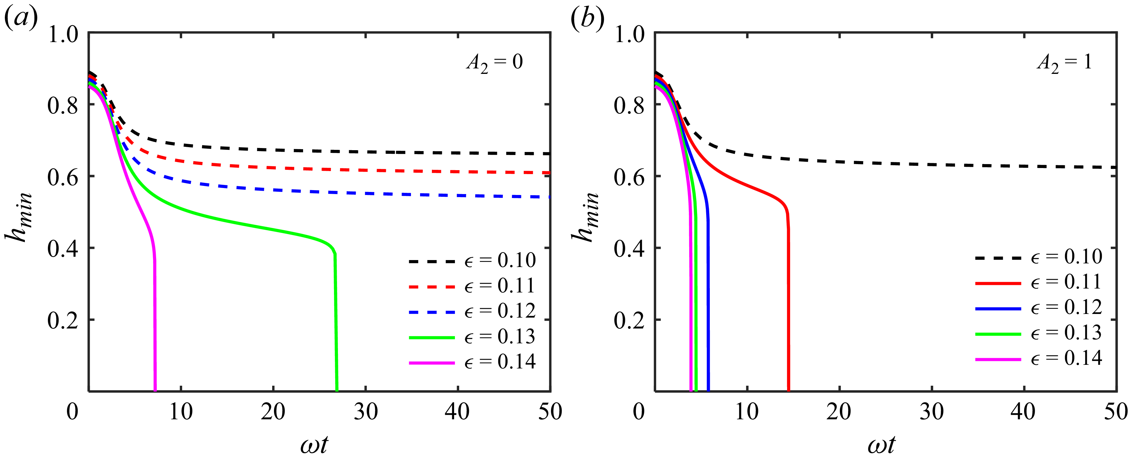
Evolution of the minimum radii of films
 $h_{ min}(t)$
for different
 $\epsilon$
while
 $A_1=0$
, for (
 $a$
)
 $A_2=0$
, (
 $b$
)
 $A_2=1$
. Dashed lines indicate the film remaining stable collars, and solid lines indicate the film forming a plug. Time scaling
 $\omega t$
follows (2.15).

It has been observed that thicker liquid films collapse through axial coalescence to form liquid plugs, while thinner films do not. This behaviour was previously reported by Everett & Haynes (Reference Everett and Haynes1972) and Gauglitz & Radke (Reference Gauglitz and Radke1988), who defined a critical thickness
 $\epsilon _c = 0.12$
to determine whether a film will collapse. To examine whether vdW forces affect this critical behaviour, we simulate liquid films within a single wavelength. The initial interface profile is defined as
 $h_0= \alpha -0.01\cos (kz)$
, with
 $z\in [-\pi /k,\pi /k]$
, where
 $k$
represents the dominant wavenumber obtained from the Stokes model (2.15). Figure 6 shows the temporal evolution of the minimum thickness
 $h_{{\textit{min}}}$
for various initial film thicknesses under two conditions:
 $A_2 = 0$
and
 $A_2 = 1$
. To enable comparison on a unified time scale and emphasise late-stage differences, the horizontal axis is normalised by the linear growth rate
 $\omega$
from (2.15). As shown in figure 6(
 $a$
), for films with
 $\epsilon \gt 0.12$
,
 $h_{\textit{min}}$
undergoes a rapid decrease starting from approximately
 $h_{\textit{min}} = 0.4$
, indicating collapse. In contrast, films with
 $\epsilon \leq 0.12$
transition to slow deformation and do not collapse within extended simulation times. The phenomenon occurs because the driving surface tension is dissipated by increasing viscous resistance near the wall, while the interfacial pressure gradient becomes insufficient to sustain further radial evolution. These findings align with earlier conclusions reported by Lister et al. (Reference Lister, Rallison, King, Cummings and Jensen2006) and Dietze & Ruyer-Quil (Reference Dietze and Ruyer-Quil2015). However, when vdW forces between liquid interfaces are present (
 $A_2 = 1$
), figure 6(
 $b$
) shows that films with
 $\epsilon = 0.11$
and
 $0.12$
shift from non-collapsing to collapsing behaviour, indicating a reduction in the critical collapse thickness
 $\epsilon _c$
.
To derive the theoretical solution for
 $\epsilon _c$
, we incorporate the vdW force term into the model developed by Gauglitz & Radke (Reference Gauglitz and Radke1988). This model assumes uniform interfacial pressure, derived as a quasi-static simplification of (2.8), expressed as
 \begin{equation} p=\frac {h''}{\bigl(1+h'^2\bigr)^{3/2}}-\frac {1}{h\sqrt {1+h'^2}} +\frac {A_1}{(1-h)^3} -\frac {A_2}{(2h)^3}=\textit{const}. \end{equation}
The resulting governing equation is an ordinary differential equation for
 $h$
, where the prime denotes differentiation with respect to
 $z$
. The left-hand side represents the total pressure. The first two terms on the right-hand side correspond to the Laplace pressure induced by interface curvature, and the last two terms describe the disjoining pressure arising from vdW forces. Assuming collar symmetry and zero film thickness at
 $z=0$
, the boundary conditions are specified as
 $h(0)=1$
and
 $h'(0)=0$
, with
 $h''(0)$
remaining an undetermined parameter. Unfortunately, non-zero
 $A_1$
leads to numerical divergence without appropriate initial guesses. Since collapse dynamics are primarily governed by interactions between opposing liquid–gas interfaces, particular emphasis is placed on the role of liquid–liquid vdW forces (
 $A_2$
) in determining the critical collapse regime. Solutions to (4.1) under varying initial conditions yield distinct equilibrium interface profiles and corresponding liquid film volumes. The result reveals the existence of a maximum film volume
 $V_{\textit{max}}$
for each vdW force. Detailed analysis of the film profile and volume are provided in Appendix C. Notably, increasing
 $A_2$
reduces
 $V_{\textit{max}}$
, indicating that a smaller liquid volume can be sustained in stable equilibrium under stronger liquid–liquid attractions.
The initial liquid film is treated as a hollow cylinder with cross-sectional area
 $\pi \bigl [1 - (1 - \epsilon )^2\bigr ]$
and dominant wavelength
 $\lambda _{\textit{max}}(\epsilon ,A_2)$
determined by (2.15). Due to volume conservation within a single wavelength, the liquid volume at the critical state equals
 $V_{\textit{max}}$
, which gives the theoretical critical thickness
 $\epsilon _c$
through the relation
 \begin{equation} V_{\textit{max}}=\pi \bigl[1-(1-\epsilon _{c})^2\bigr]\, \lambda _{\textit{max}}(\epsilon _{c},A_2). \end{equation}
The critical collapse thickness
 $\epsilon _c$
varies with the strength of liquid–liquid vdW forces
 $A_2$
when
 $A_1=0$
. The theoretical predictions from (4.1)–(4.2) are shown as a black curve, while simulation results indicating the upper and lower bounds of collar or plug are represented by symbols.

Using this theoretical framework, we construct a phase diagram that predicts the collapse behaviour of liquid films, as shown in figure 7. Collapse occurs in the orange region above the theoretical curve (black solid line), while non-collapsing films correspond to the blue region below the curve. The vdW forces between liquid–gas interfaces (
 $A_2$
) enhance interfacial attraction towards the centre axis, thereby reducing the critical thickness
 $\epsilon _c$
required for collapse. To validate the theoretical predictions, lower bounds for collapse and upper bounds for non-collapse, respectively, are determined through simulations conducted within finite time scales. The numerical results show good agreement with theory in figure 7. The slight overestimation in simulations arises from late-stage interface evolution. At this stage, the profile deviates from the idealised single-wave shape in (4.1), retaining volume in satellite lobes. Additionally, when multiple waves coexist axially, deviations from
 $\lambda _{\textit{max}}$
occur, and volume is exchanged between collars. These mechanisms may collectively reduce the effective critical thickness
 $\epsilon _c$
, a practical effect previously noted by Rykner et al. (Reference Rykner, Saikali, Bruneton, Mathieu and Nikolayev2024).
5. Interface evolution at the linear stage
After describing the overall evolution characteristics of the liquid film, we quantitatively investigate the dynamics at each regime. When perturbation amplitudes are small, the interface morphology is approximately sinusoidal, termed the linear stage. Building on linear instability analysis and numerical verification via simulations, this section examines how the liquid film evolves during the linear stage. The influence of vdW forces on the dominant wavelength is examined in § 5.1, and their effect on perturbation growth rate is discussed in § 5.2.
5.1. Dominant wavelength
Interface profiles at four time instants illustrated in different colours, with film thickness (
 $a$
,
 $b$
)
 $\epsilon =0.1$
under different
 $A_1$
, and (
 $c$
,
 $d$
)
 $\epsilon =0.5$
under different
 $A_2$
.

The root mean square
 $|H_{rms}|$
of non-dimensional perturbation amplitude versus wavenumber
 $k$
at corresponding time instants under the same conditions as in figure 8. The dash-dotted lines with circles are extracted from numerical simulations fitted by the Gaussian function (solid lines). The insets show the time histories of the dominant wavenumber converging to
 $k_{\textit{max}}$
(red dashed lines) extracted from the spectra.

To quantitatively validate the influence of vdW forces on the dominant wavelength
 $\lambda _{{\textit{max}}}$
, we simulate liquid films with various initial thicknesses under different values of
 $A_1$
and
 $A_2$
. The axial length of the computational domain is set to approximately 10 times
 $\lambda _{{\textit{max}}}$
to sufficiently resolve the wave distribution, maintaining consistency with the simulation configuration used in figure 5. Under the combined action of surface tension and vdW forces, the initially small random perturbations gradually develop into well-defined capillary waves. Figure 8 shows the evolution of the interface profile
 $h(z,t)$
under four distinct parameter conditions, with the same initial perturbation form
 $N(z)$
used across all cases to isolate parameter effects. Both
 $A_1$
(figures 8
 $a$
,
 $b$
) and
 $A_2$
(figures 8
 $c$
,
 $d$
) accelerate the evolution rate and reduce the capillary wavelength.
To compare numerical results with theoretical predictions from the Stokes model (2.15), we conduct multiple independent simulations (30 realisations per parameter) with different random initial conditions to statistically determine the dominant wavelength
 $\lambda _{{\textit{max}}}$
. For each realisation, we use the discrete Fourier transform of the interface profile
 $h(z,t)$
to obtain the power spectral density (PSD) of the perturbations. This statistical methodology, introduced by Zhao, Sprittles & Lockerby (Reference Zhao, Sprittles and Lockerby2019), has been successfully applied to characterise dominant instability modes in various liquid film systems (Zhao et al. Reference Zhao, Liu, Lockerby and Sprittles2022, Reference Zhao, Zhang and Si2023). Figure 9 displays the square root of the ensemble-averaged PSD, denoted as
 $H_{{rms}}$
, at each time step for the conditions corresponding to figure 8. A Gaussian function is fitted to the modal distribution spectrum, with the spectral peak identifying the wavenumber
 $k_{{rms}}$
. The insets illustrate the temporal evolutions of
 $k_{{rms}}$
extracted from simulations, showing rapid convergence to a stable value that we define as the dominant wavenumber
 $k_{{\textit{max}}}$
. Consistent with the observations in figure 8, the dominant wavenumbers in figures 9(
 $b$
,
 $d$
) with vdW forces are significantly larger than those in figures 9(
 $a$
,
 $c$
) without vdW forces, confirming the wavelength-reducing effect of the intermolecular interactions.
Based on the preceding analysis, we present the simulated values of
 $\lambda _{{\textit{max}}}$
for various parameter combinations in figure 10, as well as experimental data from Tomo et al. (Reference Tomo, Nag and Takamatsu2022). Both numerical results and experimental measurements demonstrate excellent agreement with our theoretical model, confirming that the proposed theoretical framework accurately captures the physical mechanism of instability across a wide parameter range. Furthermore, the results clearly show that vdW forces significantly reduce the dominant wavelength during the linear evolution stage of liquid films, with this effect being pronounced over a broad spectrum of conditions. In general, thinner films are more sensitive to solid–liquid vdW forces (
 $A_1$
), while thicker films show earlier and more substantial influence from liquid–liquid vdW forces (
 $A_2$
).
Effects of vdW forces (
 $a$
)
 $A_1$
and (
 $b$
)
 $A_2$
on the dominant wavelengths
 $\lambda _{ max}$
: a comparison between the theoretical predictions of (2.15) (solid lines) and results of numerical simulation (Sim.) from the spectra (hollow symbols) with different film thickness
 $\epsilon$
. The solid diamonds represent experimental results (Exp.) by Tomo et al. (Reference Tomo, Nag and Takamatsu2022).

5.2. Perturbation growth
During the linear stage of liquid film evolution, the interface profile under the small perturbation assumption follows
 $h(z,t) = \alpha + \hat {h}\textrm{e}^{\omega t+\textrm{i}kz}$
, where
 $\hat {h}$
represents the initial perturbation amplitude at
 $t=0$
. To validate the theoretical predictions, we simulated a perturbed liquid film within one dominant wavelength, initialising the interface as
 $h_0 = \alpha - 10^{-3} \cos({kz})$
. The early-stage evolution results, presented in figure 11, demonstrate excellent agreement with the Stokes model (2.15). Additionally, the simulations confirm that vdW forces accelerate perturbation growth during the linear instability development of liquid films.
Linear time evolution of the minimum radii of films
 $h_{ min}$
with various (
 $a$
)
 $A_1$
, where the maximum growth rate is
 $\omega =0.094,0.306,1.433,3.041$
, respectively; (
 $b$
)
 $A_2$
, for
 $\omega =0.094,0.367,1.823,3.879$
, respectively. The numerical solutions (circles) are compared with the predictions of the Stokes model (solid lines). Here,
 $\epsilon =0.5$
,
 $\hat {h}=10^{-3}$
.

Furthermore, predicting the time to reach singularity is valuable for both computational modelling and practical applications. These times are denoted as
 $t_r$
for rupture and
 $t_c$
for collapse in liquid films under vdW forces. We estimate the singularity time based on the linear stage, which is easily predicted and usually accounts for the vast majority. This method has been previously applied to film rupture on planar substrates and film collapse (Martínez-Calvo et al. Reference Martínez-Calvo, Moreno-Boza and Sevilla2021; Rykner et al. Reference Rykner, Saikali, Bruneton, Mathieu and Nikolayev2024). The specific formulas used are
 $t_r=[\ln (\epsilon /\hat {h})]/\omega ,\ t_c=[\ln (1-\epsilon )/\hat {h}]/\omega$
, where
 $\omega$
is the corresponding linear growth rate according to (2.15). In our simulations, the initial interface configuration is the same as the case used for growth rate validation. Figure 12 compares the simulated rupture and collapse times with theoretical predictions. Overall, the linear growth rate based theory captures both the trend and magnitude of the evolution duration. Regarding the role of vdW forces, solid–liquid interactions (
 $A_1$
) reduce the rupture time, as shown in figure 12(
 $a$
). For small
 $A_1$
, thinner films do not rupture more rapidly due to their weak curvature effects, which limit the growth rate. In contrast, large
 $A_1$
values significantly accelerate film evolution and promote earlier rupture. Meanwhile, liquid–liquid interfacial interactions (
 $A_2$
) consistently shorten the collapse time across all film thicknesses, as is intuitively expected and demonstrated in figure 12(
 $b$
). Theoretical predictions slightly overestimate the simulation results generally, as interface evolution accelerates in the nonlinear regime relative to the linear growth rate. However, near the critical collapse thickness (figure 12
 $b$
), simulations show significant deviations. This discrepancy stems from a viscous blocking phenomenon – identified by Dietze & Ruyer-Quil (Reference Dietze and Ruyer-Quil2015) – in which the thin liquid film between adjacent collars strongly inhibits further evolution. Consequently, the film remains in a prolonged quasi-stable state during the nonlinear stage before undergoing rapid collapse, as seen in the late-time evolution shown in figure 6.
Linear prediction of (
 $a$
) rupture time
 $t_r$
and (
 $b$
) collapse time
 $t_c$
. The numerical solutions (symbols) are compared with the predictions of the Stokes model (solid lines).

6. Dynamics at the nonlinear stage
As introduced in § 5, linear instability analysis is based on the assumption of small-amplitude perturbations, where the evolving interface morphology can be represented as a superposition of sinusoidal Fourier modes. However, as perturbations grow into the nonlinear regime, the interface profile progressively deviates from simple trigonometric forms. This section investigates the nonlinear stages of interface evolution under vdW forces, examining the morphology and structure immediately preceding rupture in § 6.1 and collapse in § 6.2, as well as the self-similar behaviour in § 6.3 during these processes.
6.1. Film rupture and satellite lobes
To examine the nonlinear rupture behaviour of liquid films in detail, we construct a computational domain spanning one wavelength. The initial mean thickness is set to
 $\epsilon =0.1$
, below the critical collapse thickness
 $\epsilon _c$
to ensure that rupture occurs. A sinusoidal initial profile with amplitude 0.001 is imposed. As shown in figure 13(
 $a$
), vdW forces significantly influence the late-stage morphology of the liquid film. In the absence of vdW forces, the film evolves into primary collars accompanied by satellite lobes. When vdW forces are present, large radial velocities develop at the thinnest region of the film, ultimately leading to rupture. To consistently identify satellite lobes, we define the thinnest point as satisfying
 $1-h_{{\textit{max}}} \lt 10^{-4}$
, minimising misidentification due to morphological changes from flow between primary and satellite structures. As
 $A_1$
increases, the relative length of satellite lobes gradually decreases until they fully disappear. Correspondingly, the volume ratio
 $V_{{sat}}/V$
also varies, as shown in figure 13(
 $b$
), where
 $V_{{sat}}$
is the satellite lobe volume, and
 $V$
is the total liquid volume per wavelength. As
 $A_1$
increases,
 $V_{{sat}}/V$
initially rises, peaks at approximately 0.09, then rapidly decreases to zero. Thicker films require a higher threshold of
 $A_1$
to completely suppress satellite lobe formation.
(
 $a$
) The film profile near rupture with different
 $A_1$
, for
 $\epsilon =0.1$
. (
 $b$
) Volume proportion of satellite lobes under the influence of
 $A_1$
.

Evolution of perturbation growth at the nonlinear stage with four
 $A_1$
values: (
 $a$
)
 $A_1=0$
, (
 $b$
)
 $A_1=10^{-7}$
, (
 $c$
)
 $A_1=10^{-5}$
, (
 $d$
)
 $A_1=10^{-3}$
. The contours represent the velocity magnitude
 $|{\boldsymbol{u}}|=\sqrt {u^2+w^2}$
, and the arrowed lines represent streamlines. Here,
 $\epsilon =0.1$
.

To further investigate the mechanism governing profile variation under vdW forces, we present velocity contours of
 $|{\boldsymbol{u}}| = \sqrt {u^2 + w^2}$
and corresponding streamlines at different evolution times in figure 14. In the absence of vdW forces as shown in figure 14(
 $a$
), instability is driven solely by surface tension. The film in the initially thinnest region experiences increasing adhesive effects near the wall, leading to flow deceleration. As a result, the film between developing collars bends inwards, forming secondary satellite lobe structures (Dietze & Ruyer-Quil Reference Dietze and Ruyer-Quil2015). A slow axial flow from the satellite lobe towards the primary collar persists, continually reducing the satellite lobe volume. However, vdW forces alter this evolution by introducing a molecular length scale
 $a = \sqrt {\tilde {A}/6\pi \gamma } = \sqrt {A}r_0$
(de Gennes Reference de Gennes1985). When the vdW forces are weak (
 $A_1 = 10^{-7}$
, figure 14
 $b$
), surface tension remains the dominant driving mechanism through most of the evolution, until the film thickness approaches
 $a$
. Subsequently, growing vdW attraction induces rapid rupture towards the wall at the thinnest point (figure 14
 $b$
iv), which suppresses axial flow towards the primary collars, and increases the relative volume of satellite lobes. For stronger vdW forces (figure 14
 $c$
), the region of maximum velocity (figure 14
 $c$
ii) shifts towards the symmetry axis, and the thinning neck contracts earlier. The resulting rupture produces a shorter satellite lobe (figure 14
 $c$
iv). When
 $A_1$
is further increased to
 $10^{-3}$
(figure 14
 $d$
), vdW forces dominate over surface tension, reducing the evolution time by three orders of magnitude. The film develops strong radial velocities (figure 14
 $d$
iv) before any distinct satellite structure can form, maintaining the thinnest point at the centre, and fully suppressing satellite lobe development.
Minimum film thickness
 $1-h_{ max}$
as a function of (
 $a$
) the time
 $t$
and (
 $b$
) the time remaining to rupture
 $t_r-t$
for different
 $A_1$
. The initial conditions
 $h_0= 0.9+10^{-3} \cos({kz})$
use the corresponding dominant wavenumbers.

The nonlinear dynamics is usually evaluated by temporal evolution of the minimum film thickness
 $1-h_{{\textit{max}}}$
, with particular focus on the scaling laws governing film rupture processes (Zhang & Lister Reference Zhang and Lister1999; Moreno-Boza et al. Reference Moreno-Boza, Martínez-Calvo and Sevilla2020; Calvo-Rivera et al. Reference Calvo-Rivera, Moreno-Boza and Sevilla2025). As shown in figure 15(
 $a$
), films without vdW forces thin continuously according to
 $1-h_{{\textit{max}}} \sim t^{-1/2}$
during the nonlinear stage without rupturing. Capillary and viscous forces maintain the film at a finite thickness over extended durations. This behaviour follows the scaling law reported by Lister et al. (Reference Lister, Rallison, King, Cummings and Jensen2006) for annular films in the specific configuration where a collar adjoins a lobe. When
 $A_1 \gt 0$
, the thinning behaviour deviates from the scaling law and leads to rapid rupture. The onset of this deviation occurs earlier as
 $A_1$
increases.
Based on the preceding analysis of scaling laws in liquid film rupture (Zhang & Lister Reference Zhang and Lister1999; Martínez-Calvo et al. Reference Martínez-Calvo, Moreno-Boza and Sevilla2021), we examine the evolution on the singularity time scale
 $\tau = t_r - t$
(figure 15
 $b$
). As
 $A_1$
increases, the thinning behaviour progressively approaches a
 $\tau ^{1/3}$
power law, indicating the growing dominance of vdW forces instead of surface tension. This behaviour can be explained through dimensional analysis, which constructs dimensionless relationships among the key physical quantities governing the process (Curtis, Logan & Parker Reference Curtis, Logan and Parker1982). The parametric dependence of the film thickness
 $\tilde {h}_f = r_0 - \tilde {h}$
can be expressed as
 \begin{equation} \tilde h_f =F\bigl(\tilde z, \tilde \tau , \mu , \tilde A_1\bigr), \end{equation}
where tildes denote the dimensional versions of the flow variables. Choosing
 $(\tilde \tau ,\mu , \tilde A_1)$
as the dimensional basis, the Buckingham
 $\varPi$
theorem provides the reduced functional form
 \begin{equation} \tilde h_f =\tilde {H}\left[\left(\mu /\tilde A_1 \tilde \tau \right)^{1/3} \tilde z\right]\left(\tilde A_1/\mu \right)^{1/3} \tilde \tau ^{1/3}. \end{equation}
This expression shows that as the rupture singularity is approached (
 $\tau \to 0$
), the interface evolution
 $\tilde {h}_f$
separates into two parts: a self-similar spatial profile
 $\tilde {H}$
, and a time-scaling law
 $\tilde {\tau }^{1/3}$
. Consequently, the thickness at the rupture point (
 $z=0$
) exhibits a
 $\tau$
-dependent scaling near the singularity, which leads to the dimensionless scaling relation
 \begin{equation} 1-h_{\textit{max}}\sim \tau ^{1/3}\quad\textrm{when}\ \tau \to 0. \end{equation}
The
 $\tau ^{1/3}$
scaling law for vdW-dominated rupture can be obtained by combining (6.2) and figure 15(
 $b$
), which is consistent with previous findings for thin films on planar substrates (Moreno-Boza et al. Reference Moreno-Boza, Martínez-Calvo and Sevilla2020).
6.2. Film collapse
Thin liquid films tend to rupture towards the tube wall, whereas thick films collapse towards the central axis. Collapse constitutes another type of singularity distinct from film rupture. This subsection examines how vdW forces affect the flow characteristics preceding liquid film collapse. The simulation set-up employed an initial sinusoidal interface profile within a single wavelength, with initial thickness
 $\epsilon = 0.5$
. Figure 16 shows contours of flow velocity magnitude and corresponding streamlines at different instants. The vdW forces from the liquid–liquid interaction accelerate all stages of the collapse process, and enhance internal flow velocities within the film. Moreover, as shown in figure 16(
 $c$
), vdW forces cause the flow to focus more strongly towards the tip region, and sharpen the interface profile gradient. Owing to the
 $\varPi \propto d^{-3}$
dependence of vdW forces, they drive radially dominated flow, where the tip velocity reaches approximately twice that without vdW forces.
Evolutions of perturbation growth streamlines near film collapse for
 $A_2=0$
(left) and
 $A_2=0.1$
(right). The contours represent the velocity magnitude
 $|{\boldsymbol{u}}|=\sqrt {u^2+w^2}$
, and the arrowed lines represent streamlines. Here,
 $\epsilon =0.5$
.

Minimum interface radius
 $h_{ min}$
as a function of time remaining to collapse
 $t_c-t$
for different
 $A_2$
. The initial conditions
 $h_0= 0.5-10^{-3} \cos({kz})$
use the corresponding dominant wavenumbers.

We further examine the nonlinear scaling behaviour near the collapse singularity, focusing on the evolution of the minimum point
 $h_{{\textit{min}}}$
with respect to the time to collapse
 $t_c - t$
, as shown in figure 17. In the absence of vdW forces, where viscous resistance and surface tension dominate, the film collapse initially follows
 $h_{{\textit{min}}} \sim (t_c - t)^{1/5}$
. During this early stage, the interface evolution could be described by the lubrication theory (2.17) and exhibits self-similar behaviour (Ding et al. Reference Ding, Liu, Liu and Yang2019), as the film maintains a small-amplitude morphology. This
 $1/5$
scaling law is also consistent with the initial stages of film collapse observed experimentally (Pahlavan et al. Reference Pahlavan, Stone, McKinley and Juanes2019). Subsequently, the evolution transitions to a linear scaling
 $h_{{\textit{min}}} \sim (t_c - t)$
, which aligns with the behaviour reported for bubble pinch-off in highly viscous liquids, both in capillary tubes (Pahlavan et al. Reference Pahlavan, Stone, McKinley and Juanes2019) and in large tanks (Burton, Waldrep & Taborek Reference Burton, Waldrep and Taborek2005), since these processes represent temporally localised singularities dominated by radial viscous effects. In contrast, when vdW forces are present, the collapse process converges to a
 $1/3$
power-law scaling, identical to the rupture scaling law. This indicates that vdW forces dominate the final stages of collapse, overriding the geometric constraints that govern collapse in their absence.
6.3. Self-similarity
For these singular behaviours governed by vdW forces, a unified description applicable to both rupture and collapse can be established. We rescale the system parameters using the characteristic vdW length
 $a=\sqrt {\tilde {A}/6\pi \gamma }$
(denoted by subscript
 $a$
), as
 \begin{equation} (r_a,z_a,h_a,t_a)=\frac {r_0}{a}(r,z,h,t),\quad (p_a,\boldsymbol{\sigma }_a)=\frac {a}{r_0}(p,\boldsymbol{\sigma }). \end{equation}
(
 $a$
) Extreme point of interface evolution
 $(1-h_{\textit{max}})_a$
or
 $(h_{\textit{min}})_a$
as a function of the time remaining to singular points
 $(t_r-t)_a$
or
 $(t_c-t)_a$
. The length and time are rescaled by the characteristic length
 $a=\sqrt {\tilde {A_i}/6\pi \gamma }$
, where
 $i=1,2$
for rupture and collapse, respectively. (
 $b,c$
) Self-similarity profiles at different instants
 $\tau _a$
for
 $A_1=0.1$
or
 $A_2=0.1$
, compared with theoretical solution of film on a flat substrate by Moreno-Boza et al. (Reference Moreno-Boza, Martínez-Calvo and Sevilla2020).

Figure 18(
 $a$
) shows the scaling behaviour near the singularity after this non-dimensionalisation, with rupture and collapse data corresponding to figures 15 and 17, respectively. All datasets ultimately collapse onto the universal curve
 $h_a \sim \tau _a^{1/3}$
, confirming the common scaling governing both types of singular evolution. We further hypothesise that the flow near the singularity exhibits local self-similarity, where the interface profile can be derived from (6.2), expressed as
 \begin{equation} h_a \xrightarrow {\tau _a\to 0} H\left(z_a/\tau _a^{1/3}\right)\tau _a^{1/3}. \end{equation}
Figures 18(
 $b$
,
 $c$
) present the self-similar profiles for rupture and collapse under selected parameters, with legend values indicating
 $\tau _a$
. As
 $\tau _a \to 0$
, the interface profiles converge towards a wedge-like shape with a constant opening angle. Comparison with the self-similar solution for planar film rupture reported by Moreno-Boza et al. (Reference Moreno-Boza, Martínez-Calvo and Sevilla2020) shows good agreement with our simulations in the cylindrical tube, supporting the universality of vdW-dominated singularities. However, this self-similar behaviour is only observed for a specific range of vdW forces. In other parameter regimes, the profiles do not exhibit clear self-similarity as predicted by the theoretical solution. This limitation primarily arises from the influence of cylindrical curvature, whose effect on nonlinear evolution dynamics requires more rigorous theoretical treatment in future works.
7. Conclusion
In this study, the influence of vdW forces on the instability of liquid films in cylindrical tubes is investigated systematically, encompassing both the linear stage of small perturbations and the nonlinear evolution preceding film rupture or collapse. The strengths of vdW forces from the solid–liquid and liquid–liquid interactions are characterised by the dimensionless Hamaker constants
 $A_1$
and
 $A_2$
, respectively. A theoretical model is developed based on linear stability analysis of the Stokes equations, extending beyond classical lubrication theory. Results show that the lubrication model overestimates both the dominant wavenumber
 $k_{{\textit{max}}}$
and the perturbation growth rate
 $\omega$
, whereas the proposed Stokes model provides more accurate predictions of film instability. These theoretical findings, along with further dynamic analysis, are validated through direct numerical simulation of the NS equations. When the initial film thickness
 $\epsilon$
exceeds a critical value
 $\epsilon _c$
, the film may collapse and form liquid plugs. By modelling the film under quasi-static pressure equilibrium, we derive the maximum sustainable film volume and the theoretical critical thickness
 $\epsilon _c$
. Simulation results confirm that the liquid–liquid vdW forces reduce
 $\epsilon _c$
, enabling the collapse of thinner films. During the linear stage of perturbation growth, both types of vdW forces increase
 $k_{{\textit{max}}}$
and
 $\omega$
, with ultra-thin films (
 $\epsilon \lt 0.1$
) exhibiting particularly strong wavelength reduction. The predicted trend in dominant wavelength is further supported by experimental data from Tomo et al. (Reference Tomo, Nag and Takamatsu2022). Additionally, the times to rupture (
 $t_r$
) and collapse (
 $t_c$
) can be qualitatively predicted from linear growth rates. In the nonlinear regime, vdW forces are shown to induce film rupture, motivating a comparative analysis of the morphology and scaling laws associated with rupture and collapse singularities. For rupture, increasing
 $A_1$
progressively suppresses the formation of satellite lobes by accelerating local thinning near the wall, with thicker films requiring stronger vdW forces to fully eliminate satellite lobes. Scaling analysis confirms that the minimum film thickness
 $1 - h_{{\textit{max}}}$
follows a
 $\tau ^{1/3}$
power law as
 $\tau = t_r - t \to 0$
, consistent with dimensional analysis under viscosity- and vdW-dominated regimes. Similarly, during collapse governed by
 $A_2$
, the minimum thickness
 $h_{{\textit{min}}}$
adheres to the
 $\tau ^{1/3}$
scaling with
 $\tau = t_c - t$
. Using the characteristic vdW length
 $a = \sqrt {\tilde {A} / 6\pi \gamma }$
to rescale the system, both rupture and collapse data collapse onto a unified
 $\tau ^{1/3}$
scaling curve.
In summary, a theoretical framework is established describing the evolution of liquid films under vdW forces across different stages in this work. We anticipate experimental validation of key predictions, particularly the relationships between the strength of vdW forces, dominant wavelength and satellite lobe, through controlled destabilisation of nanoscale films. The proposed framework offers promising extensions, such as incorporating thermal fluctuation effects (Fetzer et al. Reference Fetzer, Rauscher, Seemann, Jacobs and Mecke2007; Zhao et al. Reference Zhao, Sprittles and Lockerby2019) or substrate slip conditions (Liao et al. Reference Liao, Li and Wei2013; Zhao et al. Reference Zhao, Zhang and Si2023), both commonly encountered in nanoscale liquid film flows. We further expect that more detailed experimental observations of nanoscale liquid film dynamics will align with the theoretical predictions presented in this study.
Acknowledgements
Useful discussions with Dr Z. Ding are gratefully acknowledged.
Funding
This work has been supported by the National Natural Science Foundation of China (nos 12572310, 12202437, 12388101), the New Cornerstone Science Foundation through the XPLORER PRIZE, the Strategic Priority Research Programme of the Chinese Academy of Sciences (XDB0910100), the Fundamental Research Funds for the Central Universities (WK2090000086), and the Startup Programme of the University of Science and Technology of China (KY2090000156).
Declaration of interests
The authors report no conflict of interest.
Appendix A. Normal mode method of linear instability
In this appendix, the instability analysis is performed for the Stokes equations using the normal mode method. Substituting the perturbed quantities (2.14) into the mass and momentum equations (2.4)–(2.6) leads to
 \begin{align}&\qquad {\rm i}k \hat {w} + \frac {1}{r} \frac {{\rm d} (\hat {u} r)}{{\rm d} r} = 0 , \end{align}
 \begin{align}& {\rm i}k \hat {p} = -k^2 \hat {w} + \frac {1}{r}\frac {{\rm d}}{{\rm d} r} \left ( r \frac {{\rm d}\hat {w}}{{\rm d} r} \right ) , \end{align}
 \begin{align}& \frac {{\rm d} \hat p}{{\rm d} r} = -k^2 \hat {u} + \frac {{\rm d}}{{\rm d} r}\left [\frac {1}{r} \frac {{\rm d} (\hat {u} r)}{{\rm d} r}\right ] . \end{align}
With (A1)–(A3), we eliminate
 $\hat {w}$
and
 $\hat {p}$
to derive a fourth-order ordinary differential equation for
 $\hat {u}$
, as
 \begin{equation} \frac {{\rm d} }{{\rm d} r}\left \lbrace \frac {1}{r} \frac {{\rm d}}{{\rm d} r} \left [r \frac {{\rm d}}{{\rm d} r} \left (\frac {1}{r} \frac {{\rm d}(\hat {u}r)}{{\rm d}r} \right ) \right ] \right \rbrace - 2k^2 \frac {{\rm d}}{{\rm d}r}\left [\frac {1}{r} \frac {{\rm d}(\hat {u}r)}{{\rm d}r} \right ]+k^4\hat {u} = 0 . \end{equation}
The general solution to (A4) can be obtained in terms of Bessel functions:
 \begin{equation} \hat {u} = C_1 r\, K_0(kr) + C_2\, K_1(kr)+ C_3 r\, I_0(kr) + C_4\, I_1(kr) , \end{equation}
where
 $I_n$
and
 $K_n$
are modified Bessel functions of the first and second kind, respectively, with subscripts denoting their order. The constants
 $C_1{-}C_4$
are determined by boundary conditions, and
 $r\in [\alpha ,1]$
, where
 $\alpha =r_f/r_0$
is the dimensionless film position. Substituting (A5) into (A1) and (A2) gives
 \begin{align} \hat {w} = [C_1 \left ( krK_1-2K_0 \right )+ C_2& kK_0 - C_3\left (2 I_0 + kr I_1 \right ) - C_4 kI_0] / (ik) , \end{align}
 \begin{align} \hat {p} = 2& \left ( C_1 K_0 + C_3 I_0 \right ) . \end{align}
In a similar approach, the perturbed quantities for
 $\hat {u}, \hat {w}, \hat {p}$
, combined with
 $h(z,t) = \alpha + \hat {h}\,{\rm e}^{\omega t+{\rm i}kz}$
, are substituted into perturbed boundary equations (2.7)–(2.13). Linearising the boundary conditions at
 $r=\alpha$
yields
 \begin{align} &\quad\frac {{\rm d} \hat {w}}{{\rm d} r} + {\rm i}k \hat {u} = 0, \end{align}
 \begin{align} \hat {p} - 2 \frac {{\rm d} \hat {u}}{{\rm d}r} = \hat {h}&\left (-k^2+ \frac {1}{\alpha ^2}+\frac {3A_1}{ (1-\alpha )^4} + \frac {3A_2}{8 \alpha ^4} \right )\!, \end{align}
 \begin{align} &\qquad\omega \hat {h} = \hat {u} . \end{align}
And at the tube wall
 $r=1$
, the no-slip and no-penetration conditions linearise to
 \begin{align} \hat {u} = 0, \quad \hat {w} = 0 . \end{align}
According to (A10),
 $\hat {h}$
in (A9) can be eliminated, reducing the system to four boundary conditions: (A8), (A9) and (A11). Substituting the Bessel functions solutions (A5)–(A7) into these perturbed equations yields a homogeneous linear system for the coefficients
 $C_1{-}C_4$
. For non-trivial solutions to exist, the determinant of the coefficients must vanish:
 \begin{equation} \begin{array}{|cccc|} F_{11} & F_{12} & F_{13} & F_{14} \\[3pt] 2\,K_0(k)-k\,K_1(k) & -k\,K_0(k) & 2\, I_0(k)+k\, I_1(k) & k\,I_0(k) \\[3pt] K_0(k) & K_1(k) & I_0(k) & I_1(k) \\[3pt] k \alpha\, K_0(k \alpha ) - K_1(k\alpha ) & k\, K_1(k\alpha ) & k \alpha\, I_0(k \alpha ) + I_1(k \alpha ) & k\, I_1(k\alpha ) \\ \end{array} =0 , \end{equation}
where
 \begin{align} F_{11} & = \left[-k^2 + 1/\alpha ^2+3A_1/(1-\alpha )^4 +3A_2/8\alpha ^4 \right] \alpha\, K_0(k \alpha ) - 2 \omega k \alpha\, K_1(k \alpha ), \nonumber \\ F_{12} & = \left[-k^2 + 1/\alpha ^2+3A_1/(1-\alpha )^4 +3A_2/8\alpha ^4 \right] K_1(k \alpha ) - 2 \omega \left [ k\, K_0(k \alpha ) + K_1(k \alpha )/\alpha \right ], \nonumber \\ F_{13} & = \left[-k^2 + 1/\alpha ^2+3A_1/(1-\alpha )^4 +3A_2/8\alpha ^4 \right]\alpha\, I_0(k\alpha ) + 2 \omega k \alpha\, I_1(k\alpha ) , \nonumber \\ F_{14} & = \left[-k^2 + 1/\alpha ^2+3A_1/(1-\alpha )^4 +3A_2/8\alpha ^4 \right] I_1(k \alpha ) + 2 \omega \left [ k\,I_0(k \alpha ) - I_1(k \alpha )/\alpha \right ]\!. \end{align}
Because
 $\omega$
only appears linearly in the first line of the determinant, the dispersion relation between
 $\omega$
and
 $k$
can be expressed explicitly as
 \begin{align} &\omega = -\frac {1}{2}\left ( k^2- \frac {1}{\alpha ^2} - \frac {3A_1}{ (1-\alpha )^4} - \frac {3A_2}{8 \alpha ^4} \right ) \nonumber \\ &\times \frac {K_0(k \alpha ) \alpha \varDelta _1 - K_1(k \alpha ) \varDelta _2 + I_0(k \alpha ) \alpha \varDelta _3 -I_1(k \alpha ) \varDelta _4}{k \alpha K_1(k \alpha ) \varDelta _1\!- \left [ k K_0(k \alpha )\!+\!K_1(k \alpha )/\alpha \right ]\! \varDelta _2\! -k \alpha I_1(k \alpha ) \varDelta _3\! + \left [ k I_0(k \alpha ) -I_1(k \alpha )/\alpha \right ]\! \varDelta _4} , \end{align}
where
 \begin{align} \varDelta _1& = \begin{array}{|ccc|} -k\,K_0(k) & 2\, I_0(k)+k\, I_1(k) & k\,I_0(k) \\[3pt] K_1(k) & I_0(k) & I_1(k) \\[3pt] k\, K_1(k\alpha ) & k \alpha\, I_0(k \alpha ) + I_1(k \alpha ) & k\, I_1(k\alpha ) \\[3pt] \end{array}\,, \nonumber \\ \varDelta _2 &= \begin{array}{|ccc|} 2\,K_0(k)-k\,K_1(k) & 2 \,I_0(k)+k\, I_1(k) & k\,I_0(k) \\[3pt] K_0(k) & I_0(k) & I_1(k) \\[3pt] k \alpha\, K_0(k \alpha ) - K_1(k\alpha ) & k \alpha\, I_0(k \alpha ) + I_1(k \alpha ) & k\, I_1(k\alpha ) \\ \end{array}\,, \nonumber\\ \varDelta _3 &= \begin{array}{|ccc|} 2\,K_0(k)-k\,K_1(k) & -k\,K_0(k) & k\,I_0(k) \\[3pt] K_0(k) & K_1(k) & I_1(k) \\[3pt] k \alpha\, K_0(k \alpha ) - K_1(k\alpha ) & k\, K_1(k\alpha ) & k\, I_1(k\alpha ) \\ \end{array}\,, \nonumber\\ \varDelta _4 &= \begin{array}{|ccc|} 2\,K_0(k)-k\,K_1(k) & -k\,K_0(k) & 2\, I_0(k)+k\, I_1(k) \\[3pt] K_0(k) & K_1(k) & I_0(k) \\[3pt] k \alpha\, K_0(k \alpha ) - K_1(k\alpha ) & k\, K_1(k\alpha ) & k \alpha\, I_0(k \alpha ) + I_1(k \alpha ) \\ \end{array}\,. \end{align}
Appendix B. Lubrication model of linear instability
In this appendix, the governing equations and corresponding dispersion relations for the lubrication model in a cylindrical tube are performed. To get the lubrication equations from the axisymmetric NS equations, we need to establish the leading-order terms by their asymptotic expansion of
 $\varepsilon$
, where
 $\varepsilon \ll 1$
. The parameters are rescaled as
 \begin{equation} \tilde {r}=\varepsilon \tilde {\lambda }r,\quad\tilde {z}=\tilde {\lambda }z,\quad\tilde {u}=\frac {\varepsilon ^4\gamma }{\mu }u,\quad\tilde {w}=\frac {\varepsilon ^3\gamma }{\mu } w,\quad\tilde {t}=\frac {\tilde {\lambda }\mu }{\varepsilon ^3 \gamma }t,\quad\tilde {p}=\frac {\varepsilon \gamma }{\tilde {\lambda }}p. \end{equation}
Here,
 $\tilde {\lambda }=r_0/\varepsilon$
represents the radial characteristic length. The Stokes equations (2.2)–(2.3) yield
 \begin{align} \frac {\partial w}{\partial z}&+ \frac {1}{r} \frac {\partial (ur)}{\partial r} =0, \end{align}
 \begin{align} \frac {\partial p}{\partial z}= \varepsilon ^2&\frac {\partial ^2 w}{\partial z^2}+ \frac {1}{r}\frac {\partial }{\partial r}\biggl (r \frac {\partial w}{\partial r}\biggr ) , \end{align}
 \begin{align} \frac {\partial p}{\partial r}=\varepsilon ^4 & \frac {\partial ^2 u}{\partial z^2}+ \varepsilon ^2\frac {\partial }{\partial r}\biggl [\frac {1}{r} \frac {\partial (wr)}{\partial r}\biggr ]. \end{align}
At the liquid–gas interface
 $r=h$
, the boundary condition (2.7) and stress balance equations (2.8)–(2.9) yield
 \begin{align} &\qquad\qquad\qquad\qquad\qquad \frac {\partial h}{\partial t}+ w \frac {\partial h}{\partial z} =u, \end{align}
 \begin{align} &p-\frac {2\varepsilon ^2}{1+\varepsilon ^2(\partial _z h)^2} \left[ \frac {\partial u}{\partial r}- \frac {\partial h}{\partial z}\biggl (\frac {\partial w}{\partial r}+\varepsilon ^2\frac {\partial u}{\partial z} \biggr )+ \varepsilon ^2\biggl ( \frac {\partial h}{\partial z}\biggr )^2\frac {\partial w}{\partial z}\right]\nonumber \\ &=\frac {\partial _z^2 h}{[1+\varepsilon ^2(\partial _z h)^2]^{3/2}}-\frac {1}{\varepsilon ^2 h\sqrt {1+(\partial _z h)^2}} +\frac {A_1}{(1-h)^3} -\frac {A_2}{(2h)^3}, \end{align}
 \begin{align} &2 \varepsilon ^2\frac {\partial h}{\partial z}\biggl ( \frac {\partial u}{\partial r}- \frac {\partial w}{\partial z}\biggr ) +\left[1-\varepsilon ^2\biggl ( \frac {\partial h}{\partial z}\biggr )^2\right]\biggl ( \frac {\partial w}{\partial r}+\varepsilon ^2 \frac {\partial u}{\partial z}\biggr )=0. \end{align}
At the liquid–solid interface
 $r=1$
, the boundary condition remains
 \begin{equation} u=0,\quad w=0. \end{equation}
We filter out the higher-order terms of
 $\varepsilon$
from the governing equations above, leading to
 \begin{align}&\qquad\qquad\qquad\quad \frac {\partial w}{\partial z}+\frac {1}{r}\frac {\partial (wr)}{\partial r}=0, \end{align}
 \begin{align}&\qquad\qquad\qquad 0=-\frac {\partial p}{\partial z}+\frac {1}{r\,\partial r}\left(r\frac {\partial w}{\partial r}\right), \end{align}
 \begin{align}&\qquad\qquad\qquad\qquad\qquad 0=\frac {\partial p}{\partial r}, \end{align}
 \begin{align}&\qquad\qquad\qquad\quad \frac {\partial h}{\partial t}+w\frac {\partial h}{\partial z}-u=0, \end{align}
 \begin{align}& p=\frac {\partial ^2 h}{\partial z^2}-\frac {1}{h}+\frac {A_1}{(1-r)^3}-\frac {A_2}{(2r)^3},\ \frac {\partial w}{\partial r}=0\quad\textrm{when}\ r=h, \end{align}
 \begin{align}&\qquad\qquad\qquad u=0,\ w=0\quad\textrm {when}\ r=1. \end{align}
Integrating (B10) from
 $r = h$
to
 $r = r$
with the boundary condition (B13) gives
 \begin{equation} \frac {1}{2}\frac {\partial p}{\partial z}\bigl(r^2-h^2\bigr)=r\frac {\partial w}{\partial r}. \end{equation}
After integrating (B15) from
 $r = 1$
to
 $r = r$
with the slip boundary condition (B14), we have
 \begin{equation} \frac {1}{2}\frac {\partial p}{\partial z}\biggl [\frac {1}{2}\bigl(r^2-1\bigr)-h^2\ln r \biggr ]=w. \end{equation}
Using (B9), (B12) and (B14) with the Leibniz integral rule, one can obtain
 \begin{equation} h\frac {\partial h}{\partial t}=\frac {\partial }{\partial z}\int ^1_h ur\,{\textrm {d}}{{r}}. \end{equation}
Substituting (B16) into the integral results in
 \begin{equation} \frac {\partial h}{\partial t}=\frac {1}{h}\frac {\partial }{\partial z}\biggl [ M(h)\,\frac {\partial p}{\partial z} \biggr ], \end{equation}
where
 \begin{equation} M(h)=(-1+4h^2-3h^4+4h^4\ln h)/16\,. \end{equation}
To compare the Stokes model (2.15) with the lubrication theory, (B18) is linearised using
 $h(z,t) = \alpha + \hat {h}\,{\rm e}^{\omega t+{\rm i}kz}$
, providing the dispersion relation
 \begin{equation} \omega =k^2 \biggl ( k^2-\frac {1}{\alpha ^2}-\frac {3A_1}{(1-\alpha )^4}-\frac {3A_2}{8\alpha ^4} \biggr )M, \end{equation}
where
 $M=(-1+4\alpha ^2-3\alpha ^4+4\alpha ^4\ln \alpha )/16$
.
Appendix C. Equilibrium shape and critical volume of collars
In this appendix, we analyse the solution of the liquid–film interface equilibrium equation under different conditions, including the reason why
 $A_1 \gt 0$
is not applicable and the detailed effects of
 $A_2$
. The interface equation is given by
 \begin{equation} p=\frac {h''}{\bigl(1+h'^2\bigr)^{3/2}}-\frac {1}{h\sqrt {1+h'^2}} +\frac {A_1}{(1-h)^3} -\frac {A_2}{(2h)^3}=\textit{const}, \end{equation}
which is derived under quasi-static equilibrium assumptions, and constitutes a second-order ordinary differential equation for
 $h$
with respect to
 $z$
. Considering that adjacent liquid collars are connected by an ultra-thin film, we impose the following boundary conditions: at the edge of a collar (set at
 $z=0$
) we have
 $h = 1$
and
 $h' = 0$
, while the curvature-related term
 $h''$
is treated as a free parameter.
When
 $A_1 \gt 0$
, setting
 $h(0) = 1$
leads to a singularity (
 $p \to \infty$
), which is physically inconsistent for a stable collar. To approximate our case, we instead set
 $h(0) = 1 - 10^{-\beta }$
. The resulting profiles within a wavelength exhibit strong dependence on
 $\beta$
, diverging significantly from the actual physical behaviour under investigation. Moreover, since vdW forces intensify sharply as the film thins, our simulations confirm that liquid film rupture inevitably occurs at the thinnest point when
 $A_1 \gt 0$
, precluding any stable equilibrium state. Consequently, the theoretical framework above is unsuitable for analysing the influence of
 $A_1$
on the collapse thickness, and we set
 $A_1 = 0$
in the corresponding analysis.
(
 $a$
) Equilibrium shapes of a single collar for different boundary conditions (as well as interface pressures). Lines represent theoretical results, and symbols represent corresponding numerical profiles. (
 $b$
) Liquid volume
 $V$
in a collar as a function of boundary condition
 $h''(0)$
for different
 $A_2$
, where
 $V_{\textit{max}}$
indicates the maximum volume.

When considering the influence of
 $A_2$
, different values of
 $h''$
yield distinct equilibrium interface profiles
 $h(z)$
. As shown in figure 19(
 $a$
), when
 $A_2 = 0$
, the interface with
 $h''(0) = -0.4$
displays a sharper contour than that with
 $h''(0) = -0.2$
. In contrast, when
 $A_2 = 1$
, the profiles become noticeably flatter. This flattening effect arises from vdW forces between liquid interfaces, which induce a radial contraction force dependent on the distance from the interface to the
 $z$
-axis. To maintain pressure balance, the interface must adopt a more gradual curvature. Additionally, we compare the numerical profiles of stable collars obtained in the late stages of evolution under corresponding conditions. The results show good agreement with the theoretical predictions.
These morphological differences directly affect the film volume
 $V$
, as depicted in figure 19(
 $b$
). For each vdW force condition, there exists a maximum sustainable volume
 $V_{{\textit{max}}}$
. Only films with volume per wavelength
 $V \leq V_{{\textit{max}}}$
can maintain stable collar structures instead of collapsing. Furthermore, increasing
 $A_2$
reduces
 $V_{{\textit{max}}}$
, indicating that stronger intermolecular attractions enhance the film’s tendency to collapse.