


1. Introduction
Laminar–turbulent transition in supersonic boundary layers is an attractive issue of practical importance in recent decades, due to its relevance to the aerodynamic design of high-speed vehicles (Fedorov Reference Fedorov2011; Zhong & Wang Reference Zhong and Wang2012). Natural transition, usually occurring in real-flight or wind-tunnel conditions, is significantly influenced by external perturbations, greatly underpinned by an inherent linear instability mechanism (Reed, Saric & Arnal Reference Reed, Saric and Arnal1996; Saric, Reed & White Reference Saric, Reed and White2003), and to a large extent, dominated by the ensuing nonlinear dynamics (Kachanov Reference Kachanov1994). In a pioneering work on linear stability analysis in supersonic boundary layers, Mack (Reference Mack1987) reported that more than one discrete-mode solution exists, which are named the Mack first, second,  $\ldots$, modes according to the ascending order of their frequencies. The linear evolution of these modes was confirmed by a great number of subsequent numerical works (Fedorov Reference Fedorov2011; Zhong & Wang Reference Zhong and Wang2012). It was revealed by asymptotic analysis that only the Mack first mode with
 $\varTheta > \tan ^{-1} \sqrt {M^2-1}$ (where
 $\varTheta$ and
 $M$ denote the wave angle and Mach number, respectively) has a viscous nature (Smith Reference Smith1989; Liu, Dong & Wu Reference Liu, Dong and Wu2020), while the quasi-two-dimensional first and all the higher-order Mack modes are inviscid (Cowley & Hall Reference Cowley and Hall1990; Smith & Brown Reference Smith and Brown1990; Dong, Liu & Wu Reference Dong, Liu and Wu2020; Zhao, He & Dong Reference Zhao, He and Dong2023). When the unstable modes are accumulated to finite amplitudes, the nonlinear interaction among different Fourier components becomes the leading-order impact. A series of theories were established in order to probe the nonlinear-interaction mechanisms, such as the weakly nonlinear theory (Stuart Reference Stuart1958, Reference Stuart1960; Watson Reference Watson1960), triad resonance (Craik Reference Craik1971) and secondary instability (Maseev Reference Maseev1968; Herbert Reference Herbert1988). In recent decades, the nonlinear breakdown of supersonic/hypersonic boundary-layer flows has received more and more attention; see the series of numerical works by Mayer, Von Terzi & Fasel (Reference Mayer, Von Terzi and Fasel2011a); Franko & Lele (Reference Franko and Lele2013); Sivasubramanian & Fasel (Reference Sivasubramanian and Fasel2015); Chen, Zhu & Lee (Reference Chen, Zhu and Lee2017); Hader & Fasel (Reference Hader and Fasel2019); Hartman, Hader & Fasel (Reference Hartman, Hader and Fasel2021) and Song, Dong & Zhao (Reference Song, Dong and Zhao2022).
In general, there exist three typical types of nonlinear-interaction regimes in two-dimensional (2-D) (or axisymmetric) boundary-layer flows, namely the oblique-mode breakdown (OB) regime, the fundamental resonance regime and the subharmonic resonance regime.
The OB regime appears when the dominant perturbations in the early nonlinear phase are three-dimensional (3-D), referred to as oblique travelling waves. A schematic of the OB regime is shown in figure 1(a), where two dominant perturbations with the same frequency but different spanwise wavenumbers, marked by ( $1,1$) and (
 $1,-1$) (here
 $\mathcal {M}$ and
 $\mathcal {N}$ in
 $(\mathcal {M},\mathcal {N})$ represent the ratio of the frequency and spanwise wavenumber to their fundamental counterparts, respectively), are highlighted in yellow circles (in fact, the two dominant modes are not necessarily symmetric about the frequency axis; the plot is convenient for demonstration). For low-Mach-number supersonic boundary layers (roughly speaking,
 $1< M<4$), there only exists one branch of instability, the Mack first-mode instability, and the most unstable mode appears as an oblique travelling wave. Thus, in the early nonlinear phase, the most amplified linear modes are most likely to be 3-D, leading to the OB route to trigger transition to turbulence. Numerical calculations in Thumm (Reference Thumm1991), Fasel, Thumm & Bestek (Reference Fasel, Thumm and Bestek1993) and Chang & Malik (Reference Chang and Malik1994) showed that, when a pair of oblique modes as in figure 1(a) are introduced and evolve to the nonlinear phase, a stationary streak mode, (
 $0,2$), is generated and grows with a greater rate; the streak mode eventually overwhelms the introduced oblique modes and supports the amplification of the secondary instability (SI) travelling modes with a large unstable zone and high growth rates, leading to breakdown of the laminar flow and transition to turbulence. It is also observed that, in the early nonlinear phase, the growth rate of the streak mode is the same as that of the 2-D travelling mode (
 $2,0$) and the mean-flow distortion (MFD) (
 $0,0$), but its amplitude is much greater than those of the latter two. Such an extra amplification of the streak mode was recently explained using an asymptotic analysis by considering that the growth rate of the travelling Mack mode is much smaller than its wavenumber (Song et al. Reference Song, Dong and Zhao2022). It was found that the transverse and lateral perturbation velocities, showing a roll structure, are preliminarily amplified due to the nonlinear interaction of the oblique modes, but the streamwise perturbation velocity undergoes a further amplification due to the lift-up mechanism induced by the roll structure.
Parametric resonance in the frequency–spanwise-wavenumber space. (a) the OB regime; (b) the fundamental resonance regime; (c) the subharmonic resonance regime. Here,  $\omega _0$ and
 $\beta _0$ denote the fundamental frequency and spanwise wavenumber, respectively. A similar figure can be found in Hader & Fasel (Reference Hader and Fasel2019).

If the dominant perturbation in a 2-D (or axisymmetric) base flow is a 2-D travelling wave, ( $1,0$), then in the nonlinear phase, the 3-D oblique perturbations would undergo rapid amplifications due to the SI mechanism. For a hypersonic boundary layer where the Mack second mode is the most linearly amplified perturbation, the most unstable SI modes are the ones with the same frequency but non-zero spanwise wavenumbers (Sivasubramanian & Fasel Reference Sivasubramanian and Fasel2015; Chen et al. Reference Chen, Zhu and Lee2017; Hader & Fasel Reference Hader and Fasel2019). This scenario is referred to as the fundamental resonance. Based on the critical-layer theory (Wu Reference Wu2004; Zhang & Wu Reference Zhang and Wu2022), Wu, Luo & Yu (Reference Wu, Luo and Yu2016) deduced the evolution equations for the oblique modes and claimed that the 2-D mode acts as a catalyst to promote the growth of the oblique modes. The 2-D and the oblique modes are found to be phase locked. As reported by the experimental studies of Brad et al. (Reference Brad, Thomas, Dennis, Chou, Peter, Casper, Laura, Schneider and Johnson2009), Chou et al. (Reference Chou, Ward, Letterman, Schneider, Luersen and Borg2011) and Chynoweth et al. (Reference Chynoweth, Schneider, Hader, Fasel, Batista, Kuehl, Juliano and Wheaton2019), the streak component in this regime is always much greater than the other SI modes, forming longitudinal streak patterns. This phenomenon was later confirmed by the SI analysis based on a base flow including the saturated Mack second mode (Chen et al. Reference Chen, Zhu and Lee2017; Xu et al. Reference Xu, Liu, Mughal, Yu and Bai2020).
For a subsonic or incompressible boundary layer, the most unstable Tollmien–Schlichting mode is two-dimensional, proven by the Squire theorem, and its nonlinear saturation also leads to the rapid amplification of the SI oblique mode. Both numerical calculations (Herbert Reference Herbert1988) and experimental observations (Saric, Kozlov & Levchenko Reference Saric, Kozlov and Levchenko1984) suggested that the frequency of the most unstable SI modes in the low-speed boundary layers is half that of the dominant 2-D mode, rendering a subharmonic resonance nature. For supersonic boundary layers, Kosinov, Maslov & Shevelkov (Reference Kosinov, Maslov and Shevelkov1990), Kosinov et al. (Reference Kosinov, Semionov, Shevel'kov and Zinin1994) and Kosinov & Tumin (Reference Kosinov and Tumin1996) reported a generalised subharmonic regime, for which the dominant perturbation is a 3-D first mode, and the two most promoted SI modes are subharmonic in frequency. This scenario was later confirmed by the numerical simulations in Mayer, Wernz & Fasel (Reference Mayer, Wernz and Fasel2011b).
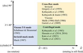
Boundary layers over a rotating disc or a rotating cone are representative 3-D boundary layers, whose linear instability for an incompressible configuration has been studied by a series of works (see Reed & Saric (Reference Reed and Saric1989), Kobayashi (Reference Kobayashi1994), Saric et al. (Reference Saric, Reed and White2003) and the references therein). For a rotating cone in a still fluid, the half-apex angle  $\theta$ is a key factor influencing the instability characteristics. As reported by Gregory et al. (Reference Gregory, Stuart, Walker and Bullard1955), Kobayashi, Kohama & Takamadate (Reference Kobayashi, Kohama and Takamadate1980), Kobayashi & Izumi (Reference Kobayashi and Izumi1983), Hussain, Garrett & Stephen (Reference Hussain, Garrett and Stephen2014) and Kato et al. (Reference Kato, Segalini, Alfredsson and Lingwood2021), the cross-flow and the centrifugal instability dominate the linear instability for a broad cone (
 $\theta > 40^{\circ }$) and a slender cone (
 $\theta < 40^{\circ }$), respectively. For a broad cone, the cross-flow instability at the upper-branch neutral point is driven by an inviscid regime, associated with the inflectional point of the base flow, whereas that at the lower-branch neutral point is driven by the balance of the viscosity, pressure gradient and Coriolis force in the near-wall region, which is a viscous mode (Hall Reference Hall1986; Malik Reference Malik1986; Garrett, Hussain & Stephen Reference Garrett, Hussain and Stephen2009). For a slender cone inserted into an axial flow, increase of the axial velocity leads to a suppression of the centrifugal instability (Kobayashi, Kohama & Kurosawa Reference Kobayashi, Kohama and Kurosawa1983; Hussain et al. Reference Hussain, Garrett, Stephen and Griffiths2016; Tambe et al. Reference Tambe, Schrijer, Gangoli and Veldhuis2021) but an enhancement of the travelling Tollmien–Schlichting wave (Schubauer & Skramstad Reference Schubauer and Skramstad1943). The compressible effect on the linear instability of rotating discs or cones was considered by Turkyilmazoglu, Cole & Gajjar (Reference Turkyilmazoglu, Cole and Gajjar2000), Turkyilmazoglu (Reference Turkyilmazoglu2005), Towers & Garrett (Reference Towers and Garrett2012, Reference Towers and Garrett2016) and Towers (Reference Towers2013). In the design of spinning projectiles in defence applications, a rotating slender cone with a supersonic axial flow is a more relevant model. The rotation-induced Magnus effect was studied by Sturek et al. (Reference Sturek, Dwyer, Kayser, Nietubicz, Reklis and Opalka1978) and Klatt, Hruschka & Leopold (Reference Klatt, Hruschka and Leopold2012), but the flow instability mechanism and transition to turbulence are not well understood. Very recently, Song & Dong (Reference Song and Dong2023) performed a systematic study on the linear instability of a Mach-3 boundary layer over a slender rotating cone with
 $7^{\circ }$ half-angle, which reported the appearance of the Mack mode (MM), the cross-flow mode (CFM) and the centrifugal mode (CM) as the rotation rate
 $\bar \varOmega$ (defined as the ratio of the rotation velocity to axial-flow velocity) increases. The aforementioned linear instability regimes for a rotating-cone configuration are summarised in figure 2, where the relevant references are also shown.
Sketch of the instability modes in the  $\theta$–
 $\bar \varOmega$ space.

As the instability modes accumulate to finite amplitudes, the nonlinear interaction among different Fourier perturbations and the MFD become dominant, which determines the nonlinear route to trigger transition. Based on the nonlinear critical-layer analysis, Gajjar (Reference Gajjar2007) studied the upper-branch cross-flow instability on an incompressible rotating-disc boundary layer, driven by inflectional base flow. The lower-branch nonlinear instability was studied by Turkyilmazoglu (Reference Turkyilmazoglu2007) based on the triple-deck theory, for which the leading-order balance appears among the convection, the viscosity and the Coriolis force. However, both of the aforementioned works are insufficient to reveal the nonlinear interaction of the instability modes in a supersonic rotating-cone boundary layer. First, as mentioned above, the instability regimes for incompressible and supersonic 3-D boundary layers are different, and so the asymptotic descriptions in Gajjar (Reference Gajjar2007) and Turkyilmazoglu (Reference Turkyilmazoglu2007) do not apply to supersonic regimes. Second, the nonlinear phase is usually reached upstream of the upper-branch neutral point, for which the linear growth rate is moderate, disagreeing with the assumptions in the critical-layer analysis. Therefore, in this paper, we will focus on the nonlinear evolution of supersonic rotating-cone modes by employing the nonlinear parabolised stability equation(NPSE), and the effect of the cone rotation on the nonlinear evolution of the travelling MMs will be particularly highlighted. In addition to the convective instability, the rotating-disc or rotating-cone boundary layers may support the absolute instability (Lingwood Reference Lingwood1995, Reference Lingwood1996). However, as reported by Garrett & Peake (Reference Garrett and Peake2007) and Garrett, Hussain & Stephen (Reference Garrett, Hussain and Stephen2010), the critical Reynolds number for the absolute instability increases remarkably as the axial-flow velocity increases, and/or the apex angle of the rotating cone decreases. Therefore, for a supersonic boundary layer over a rotating slender cone, the absolute instability is not likely to appear. Thus, in this paper, we only focus on the convective instability.
The rest of this paper is structured as follows. In § 2, we introduce the physical model, the mathematical description and the numerical treatment. The numerical results of the base flow and the linear instability analysis are provided in § 3. The nonlinear evolution of the boundary-layer instability modes is provided in § 4, in which three types of nonlinear regimes are studied in detail. The crucial role of the streak component is highlighted in § 5 and the effect of the rotation rate on transition is discussed in § 6. In § 8, we provide the concluding remarks.
2. Mathematical details
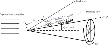
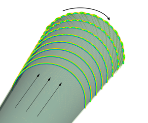
The physical model to be studied is a supersonic boundary layer over a sharp rotating cone inserted into a uniform supersonic stream with zero angle of attack, as sketched in figure 3. The half-apex angle of the cone  $\theta$ is small, which is taken to be
 $7^{\circ }$ in this paper because it is representative in wind-tunnel experiments (Schuele, Corke & Matlis Reference Schuele, Corke and Matlis2013; Craig & Saric Reference Craig and Saric2016). A viscous boundary layer forms in the vicinity of the wall. To describe the problem, the body-fitted coordinate system
 $(x^{*}, y^{*}, \varphi )$ is employed with its origin located at the cone tip, where
 $x^{*}$ and
 $y^{*}$ are along and perpendicular to the generatrix, respectively, and
 $\varphi$ is the circumferential angle. Throughout this paper, the superscript
 $*$ denotes the dimensional quantities. To study the effect of the cone rotation on the instability nonlinear evolution, we choose a number of case studies with different rotation rates. For each case study, the NPSE calculation is carried out from the same initial position with the same initial perturbations introduced. The initial position is an arbitrarily chosen position for convenience of comparison, but in § 7 we will show that the qualitative results are not affected if this initial position is changed.
Sketch of the physical model, where the NPSE calculation starts from  $x_0^*$, and marches downstream until its blowup, as marked in the blue dashed box.

The velocity field  ${\boldsymbol{u}}=(u,v,w)$, density
 $\rho$, temperature
 $T$, pressure
 $p$, dynamic viscosity
 $\mu$ are normalised by
 ${U^{*}_e}$,
 $\rho ^{*}_e$,
 $T^{*}_e$,
 $\rho ^{*}_e{U^{*2}_e}$ and
 $\mu ^*_e$, respectively, where
 ${U^{*}_e}$,
 $T^{*}_e$,
 $\rho ^{*}_e$ and
 $\mu ^*_e$ are the velocity, temperature, density and dynamic viscosity at the boundary-layer edge. The unit length is taken to be the characteristic length of the boundary layer,
 $\delta ^* = \sqrt {{{x_{0}^{*}{\mu _e ^{*} }}}/{{{\rho _e ^{*} }{U_e ^{*}}}}}$, where
 $x_{0}^{*}$ measures the distance from the leading edge to the initial position of the NPSE calculations. Thus, the coordinate system and time are normalised as
 $( {x,y} ) = {{( {{x^*},{y^*}} )} / {{\delta ^*}}}$ and
 $t = {{{t^*}{\delta ^*}} / {U_e ^*}}$, respectively. The flow is governed by three characteristic parameters, the Reynolds number, the Mach number and the dimensionless angular velocity, which are defined as
 \begin{equation} R = {{\rho _e ^*U_e ^*{\delta ^*}}}/{{\mu _e ^*}} = \sqrt{{{\rho _e ^*U_e ^*{x_0 ^*}}}/{{\mu _e ^*}}},\quad M = {{U_e ^*}}/{{a_e ^*}}, \quad \varOmega = {{{\varOmega ^*}{\delta^*} }}/{{U_e ^*}},\end{equation}
where  $a^{*}_{e}$ is the sound speed at the edge of the boundary layer. For convenience, we introduce
 $X=x/R$. Additionally, the dimensionless location of the initial position of the NPSE calculation is
 \begin{equation} x_0=x_0^*/\delta^*=R, \quad \text{or} \quad X_0=x_0/R=1, \end{equation}
and at this location the ratio of the rotating velocity to  $U_{e}^{*}$ is defined by
 \begin{equation} \bar \varOmega={\varOmega^* x_{0}^* \sin \theta }/{U^{*}_{e}}= \varOmega x_{0} \sin \theta. \end{equation}
We choose  $\bar \varOmega =O(1)$, and thus
 $\varOmega$ is only
 $O(R^{-1})$. The values of
 $\theta$,
 $M$ and
 $R$ in this paper will be introduced in table 1, and the values of
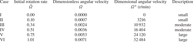
 $\varOmega$ for different case studies will be introduced in table 2.
Parameters characterising the flow condition.

Parameters of the rotation speed in this paper.

The dimensionless compressible Navier–Stokes (N-S) equations in the rotating frame  $(x,y,\varphi )$ are (Towers Reference Towers2013)
 \begin{align} \left.\begin{gathered}
\frac{{\partial \rho }}{{\partial t}} + \boldsymbol{\nabla}
\boldsymbol{\cdot} \left( {\rho {\boldsymbol{u}}} \right) =
0,\\ \rho \left[ {\frac{{{\rm D}{\boldsymbol{u}}}}{{{\rm D}
t}} + 2 \boldsymbol{\varOmega} \times {\boldsymbol{u}} +
\boldsymbol{\varOmega} \times \left(
{\boldsymbol{\varOmega} \times {\boldsymbol{r}}} \right)}
\right] ={-} \frac{\boldsymbol{\nabla} ({\rho }{T})}{\gamma
{M}^2} + \frac{1}{R}\left[ {2\boldsymbol{\nabla}
\boldsymbol{\cdot} \left( {\mu {\boldsymbol{S}}} \right) -
\frac{2}{3}\boldsymbol{\nabla} \left( {\mu
\boldsymbol{\nabla} \boldsymbol{\cdot} {\boldsymbol{u}}}
\right)} \right],\\ \frac{1}{\gamma }\rho \frac{{{\rm D}
T}}{{{\rm D} t}} - \frac{{\gamma - 1}}{\gamma }T\frac{{{\rm
D}\rho }}{{{\rm D} t}} = \frac{1}{PrR}\boldsymbol{\nabla}
\boldsymbol{\cdot} \left( {\mu \boldsymbol{\nabla} T}
\right) + \frac{{\left( {\gamma - 1} \right){M^2}}}{R}
\left[ {2\mu {\boldsymbol{S}}:{\boldsymbol{S}} -
\frac{2}{3}\mu {{\left( {\boldsymbol{\nabla}
\boldsymbol{\cdot} {\boldsymbol{u}}} \right)}^2}} \right],
\end{gathered}\right\} \end{align}
where  ${\boldsymbol {S}} = {{[ {\boldsymbol {\nabla } {\boldsymbol {u}} + {{( {\boldsymbol {\nabla } {\boldsymbol {u}}} )}^\textrm {T}}} ]} / 2}$ is the rate of the strain tensor,
 $Pr$ is the Prandtl number,
 $\boldsymbol {\varOmega }= {\varOmega } ( \cos \theta,- \sin \theta,0 )$ is the angular velocity vector,
 $\gamma$ is the ratio of the specific heats and
 ${\textrm {D}}/{\textrm {D} t} = {\partial }/{\partial t} + \boldsymbol {u} \boldsymbol {\cdot } \boldsymbol {\nabla }$ denotes the material derivative. The dimensionless equation of the state
 ${p} = {{\rho }{T}}/{\gamma {M}^2}$ has been used to eliminate the pressure
 $p$. The Sutherland viscosity law is assumed, namely,
 $\mu (T)=(1+ {C})T^{{3}/{2}}/(T+ { C})$ with
 ${ C}=110.4/{T^*_e}$ and we take
 $Pr=0.72$ and
 $\gamma =1.4$. Additionally,
 ${\boldsymbol {r}}=r(\sin \theta, \cos \theta, 0)$ is the position vector with
 $r$ being the distance to the cone axis
 \begin{equation} r=x \sin \theta + y \cos \theta. \end{equation}
The local radius of the wall is denoted by  $r_0=x \sin \theta$. The instantaneous flow field
 $\phi \equiv (\rho,u,v,w, T)$ can be decomposed into a steady base flow
 $\varPhi _B \equiv (\rho _B, U_B, R^{-1} V_B, W_B, T_B)$ and an unsteady perturbation
 $\tilde \phi$
 \begin{equation} \phi = \varPhi_B (x,y) + \tilde \phi (x,y,\varphi,t). \end{equation}
2.1. Base flow
The calculation of the base flow is the same as that in Song & Dong (Reference Song and Dong2023). Using the Mangler transformation and Dorodnitzyn–Howarth transformation
 \begin{equation} {\rm d}\bar X = {{\bar r}^2}\,{\rm d} X,\quad {\rm d}\eta = \frac{{\rho _B}\bar r\,{\rm d} y}{{\sqrt {\bar X} }}, \end{equation}
where  $\bar r=X \sin \theta$, we obtain the boundary-layer equations (BLEs)
 \begin{align} \left.\begin{gathered}
\bar X \frac{{\partial U_B}}{{\partial \bar X }} +
\frac{{\partial \bar V_B}}{{\partial \eta }} +
\frac{1}{2}U_B = 0,\\ \bar X U_B\frac{{\partial
U_B}}{{\partial \bar X }} + \bar V_B\frac{{\partial
U_B}}{{\partial \eta }} - \frac{1}{3}{\bar \varOmega
^2}{\left( {\bar W_B + 1} \right)^2}{\left( {\frac{{3\bar X
}}{{{{\sin }^2}\theta }}} \right)^{{2}/{3}}} =
\frac{\partial }{{\partial \eta }}\left( {\frac{\mu_B
}{T_B} \frac{{\partial U_B}}{{\partial \eta }}} \right),\\
\bar X U_B\frac{{\partial \bar W_B}}{{\partial \bar X }} +
\bar V_B \frac{{\partial \bar W_B}}{{\partial \eta }} +
\frac{2}{3}U_B \left( {\bar W_B + 1} \right) =
\frac{\partial }{{\partial \eta }}\left( {\frac{\mu_B
}{T_B}\frac{{\partial \bar W_B}}{{\partial \eta }}}
\right),\\ \bar X U_B\frac{{\partial T_B}}{{\partial \bar X
}} + \bar V_B\frac{{\partial T_B}}{{\partial \eta }} =
\left({\gamma - 1} \right){M^2}\frac{\mu_B }{T_B}\left[
{{{\left( {\frac{{\partial U_B}}{{\partial \eta }}}
\right)}^2} + {{\left( {\frac{{3\bar X }}{{{{\sin
}^2}\theta }}} \right)}^{{2}/{3}}}{\bar \varOmega
^2}{{\left( {\frac{{\partial \bar W_B}}{{\partial \eta }}}
\right)}^2}} \right] \\ +\, \frac{1}{{\Pr
}}\frac{\partial }{{\partial \eta }}\left( {\frac{\mu_B
}{T_B}\frac{{\partial T_B}}{{\partial \eta }}} \right),
\end{gathered}\right\} \end{align}
with  ${\bar V_B} = {{\bar r}}^{-1}{{\rho _B}\sqrt {\bar X}} ( {{V_B} + {X}^{-1}{y}{U_B}} ) + \bar X{U_B}{{ \eta }}_{{ \bar X}}$ and
 ${{\bar W}_B} = {{{W_B}}/{\bar \varOmega }}$. Note that, for a supersonic flow past a slender cone, a shock wave forms from the cone tip, after which the potential flow shows a conic-flow feature, where all the physical quantities stay almost unchanged along each ray from the cone tip. This was confirmed by performing full N-S calculations, as shown in appendix B of Song & Dong (Reference Song and Dong2023). Thus, the pressure gradient along the cone surface can be taken to be zero, which leads to
 $\rho _B T_B =1$. The boundary conditions read
 \begin{equation} \left.\begin{gathered} (U_B, \bar V_B, \bar W_B, T_B)=(0,0,0,T_w) \quad \text{at}\ \eta =0, \\ (\rho_B, U_B, \bar W_B, T_B)\rightarrow(1,1,-1,1) \quad \text{as}\ \eta \to \infty, \end{gathered}\right\} \end{equation}
where the wall is assumed to be isothermal.
The system (2.8) is parabolic with respect to  $\bar X$, which requires an initial condition at
 $\bar X=0$; this initial condition was illustrated in detail in Song & Dong (Reference Song and Dong2023). The third-order backward finite differential scheme is employed to march from
 $\bar X=0$; at each
 $\bar X$ location, the flow field is governed by a group of ordinary differential equations, which is solved by the Chebyshev collocation method.
2.2. Perturbations
Substituting the decomposition (2.6) into the N-S equations (2.4), and subtracting the base flow out, we obtain the nonlinear equations governing the disturbance
 \begin{align} & {\boldsymbol{ G }}\frac{{\partial \tilde \phi }}{{\partial t}} + {\boldsymbol{A}} \frac{{\partial \tilde \phi }}{{\partial x}} + {\boldsymbol{B}} \frac{{\partial \tilde \phi }}{{\partial y}} + {\boldsymbol{C}} \frac{{\partial \tilde \phi }}{{\partial \varphi }} + {\boldsymbol{D}}\tilde \phi + {{\boldsymbol{V}}_{xx}} \frac{{{\partial ^2}\tilde \phi }}{{\partial {x^2}}} + {{\boldsymbol{V}}_{yy}} \frac{{{\partial ^2}\tilde \phi }}{{\partial {y^2}}} \nonumber\\ &\quad +{{\boldsymbol{V}}_{\varphi \varphi }}\frac{{{\partial ^2}\tilde \phi }}{{\partial {\varphi ^2}}} + {{\boldsymbol{V}}_{xy}}\frac{{{\partial ^2}\tilde \phi }}{{\partial x\partial y}} + {{\boldsymbol{V}}_{x\varphi }}\frac{{{\partial ^2}\tilde \phi }}{{\partial x\partial \varphi }} + {{\boldsymbol{V}}_{y\varphi }}\frac{{{\partial ^2}\tilde \phi }}{{\partial y\partial \varphi }} = \boldsymbol{ F}, \end{align}
where the coefficient matrices  $\boldsymbol {G}$,
 $\boldsymbol {A}$,
 $\boldsymbol {B}$,
 $\boldsymbol {C}$,
 $\boldsymbol {D}$,
 ${\boldsymbol {V}}_{xx}$,
 ${\boldsymbol {V}}_{yy}$,
 ${\boldsymbol {V}}_{\varphi \varphi }$,
 ${\boldsymbol {V}}_{xy}$,
 ${\boldsymbol {V}}_{y \varphi }$,
 ${\boldsymbol {V}}_{x \varphi }$ and the nonlinear forcing
 $\boldsymbol {F}$ can be found in Appendix A.
2.2.1. Linear stability theory (LST)
Under the parallel-flow assumption, the perturbation  $\tilde \phi$ at each
 $x$ is expressed in terms of a travelling-wave form
 \begin{equation} \tilde \phi= {\varepsilon} \hat \phi \left( y \right){\exp[{{\rm i} \left( {\alpha x + n \varphi - \omega t} \right)}]}+ \text{c.c.}, \end{equation}
where  $\alpha$,
 $n$ and
 $\omega$ represent the streamwise wavenumber, circumferential wavenumber and frequency,
 $\textrm {c.c.}$ represents the complex conjugation,
 $\textrm {i}\equiv \sqrt {-1}$ and
 $\hat {\phi }$ denotes the normalised shape function. In what follows, the shape functions are normalised by the maximum of the streamwise velocity perturbation, such that
 ${\max }_{y} | {\hat u} | = 1$. Here,
 $\varepsilon \ll 1$ measures the amplitude of the perturbation. We are interested in the spatial mode for which only
 $\alpha = \alpha _ {r}+ \textrm {i}\alpha _ {i}$ is complex with
 $-\alpha _i$ representing its growth rate. Substituting (2.11) into (2.10) with the non-parallel terms and
 $O(\varepsilon ^2)$ terms neglected, we arrive at the compressible Orr–Sommerfeld (O-S) equation
 \begin{equation} {\boldsymbol{\tilde B}}\frac{{\partial \hat \phi }}{{\partial y}} + {{\boldsymbol{V}}_{yy}} \frac{{{\partial ^2}\hat \phi }}{{\partial {y^2}}} + {\boldsymbol{\tilde D}}\hat \phi = 0, \end{equation}
where
 \begin{equation} \left.\begin{gathered} {\boldsymbol{\tilde B}} = {\boldsymbol{B}} + {\rm{i}}\alpha {{\boldsymbol{V}}_{xy}} + {\rm{i}}n{{\boldsymbol{V}}_{y\varphi }},\\ {\boldsymbol{\tilde D}} ={-} {\rm{i}}\omega {\boldsymbol{G}} + {\rm{i}}\alpha {\boldsymbol{A}} + {\rm{i}}n{\boldsymbol{C}} + {\boldsymbol{D}} - {\alpha ^2}{{\boldsymbol{V}}_{xx}} - {n^2}{{\boldsymbol{V}}_{\varphi \varphi }} - \alpha n{{\boldsymbol{V}}_{x\varphi }} . \end{gathered}\right\} \end{equation}
The perturbation field is subject to the no-slip, isothermal boundary conditions  $\hat {u}(0)=\hat {v}(0)=\hat {w}(0)=\hat {T}(0)=0$ at the wall and the attenuation conditions
 $\hat {\phi } \to 0$ as
 $y \to \infty$. Malik's scheme (Malik Reference Malik1990) is employed to solve the linear system (2.12).
2.2.2. Parabolised stability equations (PSE)
The PSE approach (Bertolotti, Herbert & Spalart Reference Bertolotti, Herbert and Spalart1992; Chang & Malik Reference Chang and Malik1994) is considered as a more accurate means because it allows the streamwise variation of the perturbation profiles and takes into account the non-parallelism of the base flow. The only approximation is that the  $\partial _{xx}$ terms are neglected. Expressing
 $\tilde \phi$ and
 $\boldsymbol {F}$ in terms of the Fourier series with respect to
 $\varphi$ and
 $t$, we obtain
 \begin{equation} \left.\begin{gathered} \tilde \phi (x,y,\varphi,t) = \sum_{{\mathcal {M}} ={-}M_e}^{{M_e}} {\sum_{{\mathcal {N}} ={-} {N_e}}^{{N_e}} {\overset{\smile}{\phi}}_{{\mathcal {M}},{\mathcal {N}}}}(x,y) \exp [\text{i} \left({\mathcal {N}} {n_0} \varphi - {\mathcal {M}} {\omega_0} t\right)], \\ {\boldsymbol{F}} (x,y,\varphi,t) = \sum_{{\mathcal {M}} ={-}M_e}^{{M_e}} {\sum_{{\mathcal {N}} ={-} {N_e}}^{{N_e}} {{{{\boldsymbol{\tilde F}}}_{{\mathcal {M}},{\mathcal {N}}} (x,y) }{\exp [ {\text{i}\left( {{\mathcal {N}}{n_0}\varphi - {\mathcal {M}}{\omega _0}t} \right)} ] }} } , \end{gathered}\right\} \end{equation}
where  $M_e$ and
 $N_e$ denote the order of the Fourier-series truncation. In this paper, we choose
 $M_e =8$ and
 $N_e =16$, which has been confirmed to be sufficient via resolution studies (see Appendix C). Considering that the perturbations are propagating with two length scales, a fast one with an oscillatory manner and a slow one related to the non-parallelism, we express the perturbation profile
 ${\overset {\smile }{\phi }}$ as a Wentzel–Kramers–Brillouin form
 \begin{equation} {{\overset{\smile}{\phi}}_{{\mathcal {M}},{\mathcal {N}}}} (x,y) = {{\check \phi }_{{\mathcal {M}},{\mathcal {N}}}}\left( {x,y} \right) {\exp\left({{\rm i} \int_{{x_0}}^x {{\alpha _{{\mathcal {M}},{\mathcal {N}}}} (\bar x) \,{\rm d}\bar x} }\right)}, \end{equation}
where each Fourier component is denoted as  $({{\mathcal {M}},{\mathcal {N}}})$,
 $\omega _{0}$ and
 $n_{0}$ are the fundamental frequency and circumferential wavenumber, respectively, and
 $\alpha _{{\mathcal {M}},{\mathcal {N}}}$ represents the complex streamwise wavenumber of (
 ${{\mathcal {M}},{\mathcal {N}}}$). The shape function
 $\check {\phi }_{{{\mathcal {M}},{\mathcal {N}}}}$ varies slowly with
 $x$. Here,
 $x_0$ is a reference streamwise position as defined in (2.2).
Neglecting the  $\partial _{xx} \check {\phi }_{{\mathcal {M}},{\mathcal {N}}}$ terms, system (2.10) is parabolised to
 \begin{equation} {{{\boldsymbol{\tilde A}}}_{{\mathcal {M}},{\mathcal {N}}}} \frac{{\partial {{\check \phi }_{{\mathcal {M}},{\mathcal {N}}}}}}{{\partial x}} + {{{\boldsymbol{\tilde B}}}_{{\mathcal {M}},{\mathcal {N}}}} \frac{{\partial {{\check \phi }_{{\mathcal {M}},{\mathcal {N}}}}}}{{\partial y}} +{{\boldsymbol{V}}_{yy}} \frac{{{\partial ^2}{{\check \phi }_{{\mathcal {M}},{\mathcal {N}}}}}}{{\partial {y^2}}} + {{{\boldsymbol{\tilde D}}}_{{\mathcal {M}},{\mathcal {N}}}}{{\check \phi }_{{\mathcal {M}},{\mathcal {N}}}} = {{{{{\boldsymbol{\check F}}}_{{\mathcal {M}},{\mathcal {N}}}}}}, \end{equation}
where the matrices  ${{{\boldsymbol {\tilde A}}}_{{\mathcal {M}},{\mathcal {N}}}}$,
 ${{{\boldsymbol {\tilde B}}}_{{\mathcal {M}},{\mathcal {N}}}}$ and
 ${{{\boldsymbol {\tilde D}}}_{{\mathcal {M}},{\mathcal {N}}}}$ are given by
 \begin{equation} \left.\begin{gathered}
{{{\boldsymbol{\tilde A}}}_{{\mathcal {M}},{\mathcal {N}}}}
= {\boldsymbol{A}} + 2{\rm{i}}{\alpha _{{\mathcal
{M}},{\mathcal {N}}}}{{\boldsymbol{V}}_{xx}} +
{\rm{i}}{\mathcal {N}}{n_0}{{\boldsymbol{V}}_{x\varphi
}},\\ {{{\boldsymbol{\tilde B}}}_{{\mathcal {M}},{\mathcal
{N}}}} = {\boldsymbol{B}} + {\rm{i}}{\alpha _{{\mathcal
{M}},{\mathcal {N}}}}{{\boldsymbol{V}}_{xy}} +
{\rm{i}}{\mathcal {N}}{n_0}{{\boldsymbol{V}}_{y\varphi
}},\\ {{{\boldsymbol{\tilde D}}}_{{\mathcal {{\mathcal
{M}}}},{\mathcal {N}}}} ={-} {\rm{i}}M{\omega _0}
{\boldsymbol{G}} + {\rm{i}}{\alpha _{{\mathcal
{M}},{\mathcal {N}}}}{\boldsymbol{A}} + {\rm{i}}{\mathcal
{N}}{n_0}{\boldsymbol{C}} + {\boldsymbol{D}}- {{\mathcal
{N}}^2}n_0^2{{\boldsymbol{V}}_{\varphi \varphi }}\\ \quad\qquad -
\left( {\alpha _{{\mathcal {M}},{\mathcal {{\mathcal
{N}}}}}^2 - {\rm{i}}\frac{{d{\alpha _{{\mathcal
{M}},{\mathcal {N}}}}}}{{{\rm d}x}}}
\right){{\boldsymbol{V}}_{xx}} - {\mathcal {N}}{\alpha
_{{\mathcal {M}},{\mathcal
{N}}}}{n_0}{{\boldsymbol{V}}_{x\varphi }}, \\
{{{{{\boldsymbol{\check F}}}_{{\mathcal {M}},{\mathcal
{N}}}}}}= {{{{{\boldsymbol{\tilde F}}}_{{\mathcal
{M}},{\mathcal {N}}}}}}{{{\exp({-\text{i}\int_{{x_0}}^x
{{\alpha _{{\mathcal {M}},{\mathcal {N}}}}\,{\rm d}\bar x}
})}}}. \end{gathered}\right\}
\end{equation}
Such a system can be solved numerically using a marching scheme, for which the flow quantities only depend on their upstream information. Thus, as initial perturbations, a pair of oblique normal modes with the same frequency but the opposite circumferential wavenumbers is introduced at  $X=1$ (or
 $x=x_0=R$)
 \begin{equation} \tilde \phi (x_{0},y,\varphi ,t) = {\varepsilon_{1,1}} \hat\phi_{1,1}(y)E_{1,1}+ {\varepsilon_{1,-1}} \hat\phi_{1,-1}(y)E_{1,-1}+ \text{c.c.}, \end{equation}
where  $E_{{\mathcal {M}},{\mathcal {N}}}=\exp [\textrm {i} ({\mathcal {N}}n_0 \varphi -{\mathcal {M}}\omega _0 t)]$, and
 $\varepsilon _{{{\mathcal {M}},{\mathcal {N}}}}$ measures the amplitude of each mode. The shape functions of the unstable modes
 $\hat {\phi }_{{{\mathcal {M}},{\mathcal {N}}}}$ are obtained by solving numerically the compressible O-S equation (2.12). The nonlinear PSE calculation marches downstream until its blowup, indicating that the transition onset will not be far away (Dong, Zhang & Zhou Reference Dong, Zhang and Zhou2008; Mayer et al. Reference Mayer, Fasel, Choudhari and Chang2014). The wall-normal boundary conditions for the system (2.16) are
 \begin{equation} \left.\begin{gathered} ({{\check u}_{{{\mathcal {M}},{\mathcal {N}}}}},{{\check v}_{{{\mathcal {M}},{\mathcal {N}}}}}, {{\check w}_{{{\mathcal {M}},{\mathcal {N}}}}},{{\check T}_{{{\mathcal {M}},{\mathcal {N}}}}}) = (0,0,0,0) \quad \text{at}\ y = 0,\\ ({{\check \rho}_{{{\mathcal {M}},{\mathcal {N}}}}},{{\check u}_{{{\mathcal {M}},{\mathcal {N}}}}}, {{\check v}_{{{\mathcal {M}},{\mathcal {N}}}}},{{\check w}_{{{\mathcal {M}},{\mathcal {N}}}}}, {{\check T}_{{{\mathcal {M}},{\mathcal {N}}}}}) \to (0,0,0,0) \quad \text{as}\ y \to \infty. \end{gathered}\right\} \end{equation}
Because the complex streamwise wavenumber  $\alpha _{{{\mathcal {M}},{\mathcal {N}}}}$ and the nonlinear terms
 ${\boldsymbol {{\check F}}}_{{{\mathcal {M}},{\mathcal {N}}}}$ are unknown, an iterative procedure is used to solve the flow quantities at each streamwise position. More details about the iterative procedures, the discretisation scheme and code validation can be found in our previous works (Zhao et al. Reference Zhao, Zhang, Liu and Luo2016; Song et al. Reference Song, Dong and Zhao2022).
Additionally, if  $\check {\boldsymbol {F}}_{{{\mathcal {M}},{\mathcal {N}}}}$ is set to be zero, then (2.16) is recast to the linear PSE (LPSE), which can be used to track the evolution of each linear mode separately. To distinguish it, the PSE approach with
 $\check {\boldsymbol {F}}_{{{\mathcal {M}},{\mathcal {N}}}}$ retained is referred to as the nonlinear PSE (NPSE) in this paper.
2.3. Secondary instability analysis (SIA)
When the amplitude of the dominant perturbation has accumulated to a finite level, the SI may appear. In this subsection, two types of SIs are considered. The first one is based on a wavy profile driven by a saturated travelling mode, while the second one is based on a streaky profile driven by finite-amplitude longitudinal streaks.
2.3.1. The SIA for a wavy base flow
For simplicity, we assume that the perturbation field is dominated by only one travelling mode (whose frequency, streamwise wavenumber and circumferential wavenumber are denoted by  $\omega _0$,
 $\alpha _{1,1}$ and
 $n_0$, respectively) and its harmonics. When the dominant mode reaches the nonlinear saturation state, its growth rate becomes almost zero, and so
 $\alpha _{1,1}$ to leading order is almost real. The SIA is performed in the wave-propagating direction, whose oblique angle to the
 $x$ axis is
 $\varTheta =\tan ^{-1}[\beta _{1,1}/{{\alpha _{r,(1,1)}} }]$ with
 $\beta _{1,1}=n_0/r_0$. The composite wavenumber in the wave direction is given by
 $\breve \alpha = \sqrt { {\alpha ^{2}_{r,(1,1)}}+ \beta _{1,1}^{2} }$, which is also real. The base flow for the SIA is a superposition of the steady base flow and the saturated wavy travelling waves and is expressed in terms of a Fourier series. Thus, the base flow
 $\breve {\varPhi }_{B} \equiv [\breve \rho _B,\breve U_B,\breve V_B,\breve W_B,\breve T_B]$ in a moving frame reads
 \begin{equation} {\breve {\varPhi}} _{B} (\tilde x, y) = [ \rho_{B}, \tilde U-c, 0, \tilde W, T_{B}](y) + \sum_{ { m} ={-} M_{W}}^{M_{W}} {{{\overset{\smile}{\phi}} }_{m,m}}\left( y \right)\exp({\text{i} m \breve \alpha \tilde x}) +\cdots, \end{equation}
where  $c= \omega _{0}/{\breve \alpha }$,
 $\tilde x = x \cos \varTheta + z \sin \varTheta - ct$ is the Galilean transformed coordinate along the wave direction,
 $\tilde U= U_{B} \cos \varTheta +W_{B} \sin \varTheta$,
 $\tilde W=-U_{B} \sin \varTheta +W_{B} \cos \varTheta$ and
 $M_W$ denotes the order of the Fourier-series truncation. The laminar base flow
 $\varPhi _{B}$ develops with a length scale much greater than the wavelength of the fundamental mode
 $2 {\rm \pi}/ {\breve \alpha }$, and so the non-parallelism of
 $\varPhi _B$ in the local region is neglected in the present analysis. Thus,
 $\boldsymbol {\breve \varPhi }_B$ is periodic in
 $\tilde x$. We introduce the coordinate
 $\tilde z=-x \sin \varTheta + z \cos \varTheta$ to denote the direction perpendicular to the wave direction. Here,
 $\breve U_{B}$ and
 $\breve W_{B}$ are the velocities along the
 $\tilde x$- and
 $\tilde z$-directions, respectively.
According to Floquet theory, the periodic base flow supports the instability modes which can be expressed as
 \begin{equation} \left.\begin{gathered} {{\tilde \phi }(x,y,z,t)} = \varepsilon {\breve \phi _W}\left( {\tilde x,y} \right){\exp{[\text{i} \gamma_{W}( \tilde x+ct)+\text{i}\breve \beta \tilde z+{\text{i}{\sigma _d} \breve \alpha \tilde x}]}} +\text{c.c.}, \\ {\breve \phi _W}\left( {\tilde x,y} \right) = \sum_{k ={-} {N_W}}^{{N_W}} {{{\hat \phi }_{W,k}} \left( y \right)\exp \left( { \text{i} k \breve \alpha \tilde x} \right)}, \end{gathered}\right\} \end{equation}
where  $\gamma _W$ is the complex wavenumber in the
 $\tilde x$ direction with its imaginary part representing the opposite of the growth rate,
 $\breve \beta$ is the wavenumber in the
 $\tilde z$ direction,
 $\sigma _{d}$ is the detuning parameter and
 $N_W$ is the order of the Fourier-series truncation. For the fundamental resonance, we take
 $\sigma _d=0$. Here,
 $\hat {\phi }_{W,0}$ denotes the streak component, and
 $\hat {\phi }_{W,k}$ represents the travelling mode for a non-zero
 $k$ value. Substituting (2.20) and (2.21) into (2.10) with
 $O(\varepsilon ^{2})$ terms neglected forms an eigenvalue problem
 \begin{equation} [ {{{\boldsymbol{M}_0}} + \left( {\text{i}{\gamma _W}} \right) { {\boldsymbol{M}_1}} + {{\left( {\text{i}{\gamma _W}} \right)}^2} { {\boldsymbol{M}_2}} }]{ \breve \phi _W} \left( {\tilde x,y} \right) = 0,\end{equation}
where
 \begin{equation}
\left.\begin{gathered} {{\boldsymbol{M}_0}} = ( { {\boldsymbol{A}} + {\rm{i}}
\breve \beta { {{\boldsymbol{V}}_{\tilde x\tilde z}}}}) \frac{\partial }{{\partial \tilde x}} +
( {{\boldsymbol{B}} + {\rm{i}} \breve \beta { {\boldsymbol{V}_{y\tilde z}}}})\frac{\partial
}{{\partial y}} + [ { {\boldsymbol{D}} + {\rm{i}}
\breve \beta {\boldsymbol{\tilde C}} + {{( {{\rm{i}} \breve
\beta } )}^2}{ { {\boldsymbol{V}_{\tilde z\tilde z}}}}} ] \\ +\,{{\boldsymbol{V}_{xx}}}\frac{{{\partial
^2}}}{{\partial {{\tilde x}^2}}} + { {\boldsymbol{V}_{yy}}}
\frac{{{\partial ^2}}}{{\partial {y^2}}} + {
{\boldsymbol{V}_{xy}}} \frac{{{\partial ^2}}}{{\partial
x\partial y}}, \\ { {\boldsymbol{M}_1}} = ( {
{\boldsymbol{A}} + \text{i} \breve \beta {
{\boldsymbol{V}_{\tilde x\tilde z}}}} ) + 2 {
{\boldsymbol{V}_{xx}}} \frac{\partial }{{\partial \tilde
x}} + {{\boldsymbol{V}_{xy}}} \frac{\partial }{{\partial
y}} + c{\boldsymbol{G}} , \\ { {\boldsymbol{M}_2}} = {
{\boldsymbol{V}_{xx}}}, \end{gathered}\right\}
\end{equation}
with  ${\boldsymbol {\tilde C}} = {r}{\boldsymbol {C}}$,
 ${{ \boldsymbol {V}_{\tilde x \tilde z}}} = {r}{{ \boldsymbol {V}_{ x \varphi }}}$,
 ${{ \boldsymbol {V}_{y \tilde z}}}= {r}{{ \boldsymbol {V}_{ y \varphi }}}$ and
 ${{ \boldsymbol {V}_{\tilde z \tilde z}} }= {r}^{2} {\boldsymbol {V_{ \varphi \varphi }}}$. The wall-normal boundary conditions read
 \begin{equation} \left.\begin{gathered} {\breve u}_{W}= {\breve v}_{W}={\breve w}_{W}={\breve T}_{W}=0 \quad \text{at}\ y=0, \\ ({\breve \rho}_{W},{\breve u}_{W}, {\breve v}_{W},{\breve w}_{W},{\breve T}_{W}) \to 0 \quad \text{as}\ y \to \infty. \end{gathered}\right\} \end{equation}
In the  $\tilde x$-direction, the periodic boundary condition is employed. System (2.22) is discretised by using the fourth-order finite difference scheme with five points in the
 $y$-direction and the spectral method in the
 $\tilde x$-direction. A total of
 $J_W$ grid points are allocated in the wall-normal direction. The discretisation leads to a high-dimensional (the dimension of the coefficient matrix is
 $5{J_W}N_{W} \times 5{J_W}N_{W}$) eigenvalue problem with
 $\gamma _w$ being the eigenvalue, which is solved using the Rayleigh quotient iteration method (see the Appendix of Han et al. (Reference Han, Yuan, Dong and Fan2021)). In our calculations, we select
 $M_{W}=3$,
 $N_{W}=6$ and
 $J_W=581$. In general, only one unstable discrete mode exists for a given
 $\breve \beta$, and thus, we simply take the initial guess for the iteration to be
 $\gamma _w=(({(\bar \varOmega X \cos \varTheta + \sin \varTheta )}/{(-\bar \varOmega X \sin \varTheta + \cos \varTheta )}) \breve \beta,-0.01)$, which is based on the approximation that the streak direction is roughly along the potential-flow direction, and the convergence of the iteration is usually reached in 6 to 8 steps.
Such an analysis has also been used in the study of the SI of 2-D Mack second modes in a hypersonic boundary layer (Chen et al. Reference Chen, Zhu and Lee2017; Xu et al. Reference Xu, Liu, Mughal, Yu and Bai2020), and our code validation and resolution test are provided in Appendix D.
2.3.2. The SIA for a streaky base flow
Now we consider a base flow perturbed by longitudinal streaks, and the streak direction is not necessarily along the streamwise direction. We denote the angle between the streak direction and the streamwise direction by  $\theta _s$. For convenience, we introduce a coordinate transformation
 \begin{equation}
\left.\begin{array}{l@{}} {x_s} = x, \\ {z_s} = z - x\tan
{\theta _s} , \\ \end{array}\right\}
\end{equation}
which yields
 \begin{equation}
\left.\begin{array}{l@{}} \dfrac{\partial }{{\partial x}}
= \dfrac{\partial }{{\partial {x_s}}} - \tan \theta_s
\dfrac{\partial }{{\partial {z_s}}}, \\
\dfrac{\partial }{{\partial z}} = \dfrac{\partial
}{{\partial {z_s}}} . \\ \end{array}\right\}
\end{equation}
The streaky base flow obtained by NPSE can be expressed as
 \begin{equation} \breve \varPhi_{B}
(x,y,z) = \varPhi_{B} (y) +\sum_{m ={-} M_{S}}^{M_{S}}
{{{\overset{\smile}{\phi}}_{0,m}}\left( y
\right){\exp({\text{i} ( \alpha_{0,m} x +\beta_{0,m} z
)}}}) +\cdots , \end{equation}
where  $\beta _{0,m} =m n_{0}/r_{0}$ and
 $M_S$ is the Fourier-series truncation. The SIA is performed when the streak mode reaches a finite amplitude, for which the locally parallel assumption is also approximately valid. Therefore, the perturbation field
 $\tilde \phi$ can be expressed as
 \begin{equation} \left.\begin{gathered} \tilde \phi (x,y,z,t) = \varepsilon \breve{\phi}_{S}(y,z_s) \exp[{\text{ i} (\alpha_{s} x_{s}+ \sigma_{d} \beta_{0,1} z_s - \omega t)} ]+\text{c.c.}, \\ {\breve \phi _S}\left( {y,z_s} \right) = \sum_{k ={-} {N_S}}^{{N_S}} {{{\hat \phi }_{S,k}} \left( y \right)\exp \left( { \text{i} \beta_{0,k} z_s} \right)}, \end{gathered}\right\} \end{equation}
where  $\sigma _d=0$ is a detuning parameter and
 $N_S$ is the Fourier-series truncation. For the spatial mode, the frequency
 $\omega$ is real and
 $\alpha _s$ is complex, whose real and imaginary parts represent the wavenumber and the opposite of the growth rate, respectively.
Substituting (2.28), (2.27) and (2.26) into (2.10) and collecting the  $O(\varepsilon )$ terms, we obtain
 \begin{equation} [ {{ {{\boldsymbol{D}}_s}} + \text{i}{\alpha _s} {{ \boldsymbol{A}_s}} + {{\left( {\text{i}\alpha_s } \right)}^{2}} {\boldsymbol{V}_{xx}}} ] \breve \phi_S \left( {y,{z_s}} \right) = 0, \end{equation}
where
 \begin{equation} \left.\begin{gathered} {{{\boldsymbol{D}_s}}} = \boldsymbol{D} + \boldsymbol{B}\frac{\partial }{{\partial y}} + {{\boldsymbol{C}_s}}\frac{\partial }{{\partial {z_s}}} + \boldsymbol{D} \frac{{{\partial ^2}}}{{\partial {y^2}}} + {\boldsymbol{V}_{zz,s}} \frac{{{\partial ^2}}}{{\partial z_s^2}} + { \boldsymbol{V}_{yz,s}} \frac{{{\partial ^2}}}{{\partial y\partial {z_s}}} - \text{i} \omega {\boldsymbol{ G}}, \\ {\boldsymbol{A}_s} = \boldsymbol{A} + {\boldsymbol{V}_{xy}}\frac{{{\partial ^2}}}{{\partial y}} + {\boldsymbol{V}_{xz,s}}\frac{{{\partial ^2}}}{{\partial {z_s}}}, \\ \end{gathered}\right\} \end{equation}
with  ${\boldsymbol {C}_s} = {r}\boldsymbol {C} + h \boldsymbol {A}$,
 ${\boldsymbol {V}_{zz,s}} = r^2 {\boldsymbol {V}_{\varphi \varphi }}+ {r}h{\boldsymbol {V}_{x\varphi }} + {h^2}{\boldsymbol {V}_{xx}}$,
 ${\boldsymbol {V}_{yz,s}} = r {\boldsymbol {V}_{y\varphi }} + h{\boldsymbol {V}_{xy}}$,
 ${\boldsymbol {V}_{xz,s}} = r {\boldsymbol {V}_{x\varphi }} + 2h{\boldsymbol {V}_{xx}}$ and
 $h=-\tan \theta _s$. The periodic boundary condition is employed in the
 $z_s$ direction, and the same boundary conditions in the wall-normal direction as in (2.24) are employed. The numerical scheme is the same as that in § 2.3.1, and we choose
 $(M_S,N_S,J_S)=(8,16,581)$. The Arnoldi method is used to search the initial eigenvalues because a multiplicity of unstable discrete modes may exist, and the Rayleigh quotient iteration method is employed to confirm the accuracy of each eigenvalue solution. This method has been used to analyse the SI of the Görtler vortices over a concave wall in our previous work (Song, Zhao & Huang Reference Song, Zhao and Huang2020).
3. Numerical results of the base flow and its linear instability
3.1. Base flow
In the following calculations, the computational parameters are listed in table 1. Note that the values of the oncoming Mach number and temperature represent those at the outer reach of the boundary layer, and from conic-flow theory (Sims Reference Sims1964), we can estimate that the oncoming Mach number and temperature before the shock are  $M_\infty =3.214$ and
 $T_\infty =48.28$ K, respectively. A detailed verification can be seen in Song & Dong (Reference Song and Dong2023). The apex angle of the cone follows the models in the numerical studies (Zhong & Ma Reference Zhong and Ma2006; Balakumar Reference Balakumar2009; Hader & Fasel Reference Hader and Fasel2021) and the experimental studies (Schuele et al. Reference Schuele, Corke and Matlis2013; Craig & Saric Reference Craig and Saric2016), and the Mach number and the temperature of the oncoming flow are chosen from the studies of the Magnus effect in Sturek et al. (Reference Sturek, Dwyer, Kayser, Nietubicz, Reklis and Opalka1978) and Klatt et al. (Reference Klatt, Hruschka and Leopold2012). The base flow is obtained by solving numerically the BLEs (2.8) with boundary conditions (2.9) in a 2-D domain
 $\bar {X}\in [0,0.1]$ and
 $\eta \in [0,15]$, with
 $401$ and
 $121$ grid points allocated in the
 $\bar {X}$- and
 $\eta$-directions, respectively. The numerical method was also employed and confirmed to be sufficiently accurate in the study of the linear instability of a rotating-cone boundary layer in Song & Dong (Reference Song and Dong2023).
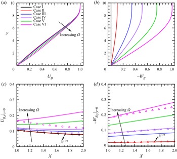
In this paper, we focus on a series of case studies with different  $\varOmega$ values, as shown in table 2, and the
 $U_B$- and
 $W_B$-profiles at
 $X=1$ are shown in figure 4(a,b), respectively. In the boundary layer, as
 $\varOmega$ increases, both
 $U_{B}$ and
 $|W_B|$ increase monotonically, leading to higher wall shears. The streamwise distributions of the wall shears of
 $U_{B}$ and
 $|W_{B}|$ are shown in figure 4(c,d), respectively. For
 $\varOmega =0$, the self-similar solution determines that the boundary-layer thickness grows like
 $X^{1/2}$, and hence the wall shear
 $U_{B}|_{y=0}$ decays like
 $X^{-1/2}$, as confirmed by the black circles. Such a scaling is not strictly satisfied as
 $\varOmega$ increases, and an appreciable discrepancy is observed when
 $\varOmega =0.0071$ for case VI. According to (b),
 $W_{B}$ is approximately proportional to
 $X$, and the boundary-layer thickness almost grows like
 $X^{1/2}$. Therefore, the wall shear of the spanwise velocity
 $-W_{B}|_{y=0}$ grows like
 $X^{1/2}$; such a scaling law is approximately correct even when
 $\varOmega =0.0071$ for case VI. The velocity profiles in the potential-flow direction
 $U_p$ and the cross-flow direction
 $U_c$ for different cases at
 $X=1$ are plotted in figure 5, where
 $U_p$ and
 $U_c$ are defined as
 \begin{align} U_p = U_B \cos \varPhi_e + W_B \sin \varPhi_e, \quad U_c ={-}U_B \sin \varPhi_e + W_B \cos \varPhi_e, \quad \varPhi_e \equiv \tan ^{{-}1} \bar \varOmega. \end{align}
As  $\varOmega$ increases,
 $U_p$ increases monotonically since
 $W_B$ induced by the rotation increases. The value of
 $U_c$ is zero at
 $y = 0$ and
 $y \to \infty$, and an inflectional point appears for
 $\varOmega \ne 0$, which is likely to support the inviscid cross-flow instability.
Base flow for different cases. (a,b) Are the profiles of  $U_B$ and
 $-W_B$ at
 $X=1.0$, respectively. (c,d) Are the streamwise distributions of the wall shears of the streamwise and spanwise velocities, respectively. The circles in (c) denote the scaling of
 $X^{-1/2}$, and the triangles in (d) denote the scaling of
 $X^{1/2}$.

Wall-normal profiles of (a)  $U_p$ and (b)
 $U_c$ at
 $X = 1$ for different cases.

3.2. Linear instability analysis
The linear instability analysis can be performed using either the LST, for which the local growth rate is predicted based on the base flow at each streamwise location, or the LPSE, for which the amplitude evolution is predicted by a marching scheme.
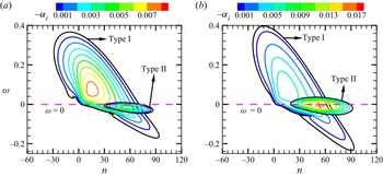
The LST analysis for a rotating cone at this Mach number in Song & Dong (Reference Song and Dong2023) reveals that, when the rotation speed is small, only one unstable zone exists, but for a sufficiently high rotation rate, an additional unstable zone near the zero-frequency band appears. To be distinguished, the unstable modes in the two zones are referred to as the type-I and type-II instabilities, respectively, following Song & Dong (Reference Song and Dong2023). Note that this notation is different from that in Garrett et al. (Reference Garrett, Hussain and Stephen2009), where the two instability types are referred to as the inviscid CFM and the viscous Coriolis mode. The type-I instability may be a MM or a quasi-stationary CFM, while the type-II instability may be a CM at a moderate  $R$ or a CFM at a large
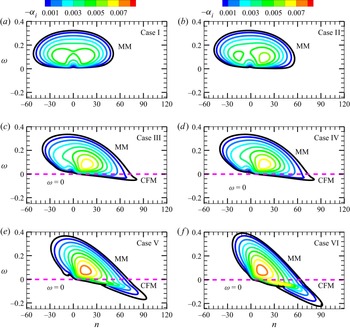
 $R$. For cases V and VI, both type-I CFM and type-II CM exist. As confirmed by figure 20 in Song & Dong (Reference Song and Dong2023), the CFM appears as a pair of co-rotating vortices near the critical line, while the CM appears as a pair of counter-rotating vortices in the near-wall region, agreeing with the experimental observations in Kobayashi et al. (Reference Kobayashi, Kohama and Kurosawa1983) and Kobayashi (Reference Kobayashi1994). The CM shows a much greater growth rate than that of the CFM. In figure 6, we show the contours of the growth rates for the type-I instability modes for different cases. For
 $\varOmega =0$, shown in (a), the unstable zone is symmetric about the
 $n=0$ line, and the most unstable mode appears as a pair of oblique waves. This mode is the Mack first mode, abbreviated as MM. When
 $\varOmega$ is slightly increased, as shown in (b), the unstable zone leans towards the positive-
 $n$ direction, also showing an MM-instability nature. For
 $\varOmega =0.0024$ and 0.0036 (cases III and IV), the right-branch unstable zone crosses the zero-frequency line, indicating the appearance of the stationary mode. Previous analysis (Song & Dong Reference Song and Dong2023) confirmed that the quasi-stationary mode is driven by the cross-flow effect, and so it is referred to as the type-I CFM, while the majority of the travelling mode is still the MM instability. As
 $\varOmega$ is further increased such that
 $\bar \varOmega$ reaches 0.75 and 1.01, the unstable zone of the type-I CFM enlarges. Simultaneously, as shown in figure 7, the type-II CM instability appears in the vicinity of the zero-frequency line, whose growth-rate peak (0.017) exceeds that of the MM instability (0.009) for case VI when
 $\bar \varOmega$ reaches 1.01.
Growth-rate contours of type-I instability in the  $\omega$–
 $n$ plane for different cases at
 $X=1$. The black contour in each panel represents the neutral curve where
 $\alpha _i=0$.

Growth-rate contours of the type-I and type-II instabilities in the  $\omega$–
 $n$ plane for cases V (a) and VI (b) at
 $X=1$.

A clearer observation by showing the dependence of the growth rate on  $\omega$ for different
 $n$ values for representative cases is shown in figure 8. For a moderate rotation rate (case IV), shown in (a), only the type-I instability appears. The curve for
 $n=25$ shows a single-peak feature, representing the MM instability, whereas for
 $n=55$, the growth rate shows two mild maxima near
 $\omega =0$, corresponding to an MM and a CFM, as marked in the plot. For a strong rotating case (case VI), shown in (b), the CFM already appears when
 $n=25$, and becomes the dominant mode for type-I instability when
 $n=55$. Additionally, the type-II CM instability appears in the low-frequency band when
 $n=55$ with a much greater growth rate.
Dependence on  $\omega$ of the growth rate
 $-\alpha _i$ for different
 $n$ values for cases IV (a) and VI (b) at
 $X=1$.

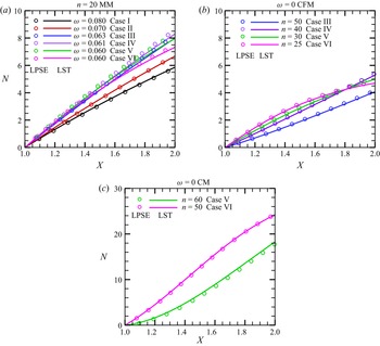
The accumulated amplitude of the instability mode at each frequency and circumferential wavenumber can be measured by an  $N$ factor, which can be predicted by the LST-predicted growth rate via
 \begin{equation} N(x) =\exp\left[\int_{{x_0}}^x { - {\alpha _i} (\tilde x) \,{\rm d}\tilde x}\right], \end{equation}
or by the LPSE-calculated amplitude via
 \begin{equation} N(x) = \ln [ {{{{A_u}\left( { x} \right)}/{{A_u}\left( {{x_0}} \right)}}} ], \end{equation}
where  $A_{u}(x)= {\max }_{y} | { {{\overset {\smile }{u}}} (x,y)} + \textrm {c.c.} |$ denotes the amplitude of the streamwise velocity disturbance. For the type-I instability, the travelling MM is always more unstable than the quasi-stationary CFM, and the most unstable MMs appear around
 $n=20$. However, the frequency of the most unstable mode varies with the angular rotation rate
 $\varOmega$. In figure 9(a), we compare the streamwise evolution of the
 $N$ factors of the type-I MM for different
 $\varOmega$ values. The greatest amplitude appears for case IV with
 $\varOmega =0.0036$, further increase or decrease of the rotation speed leads to a reduction of the accumulated amplitude. (b) Plots
 $N$-factor accumulation of the stationary type-I CFM for cases III to VI, because for smaller
 $\varOmega$ values the CFM are stable. The accumulated
 $N$ factor of the CFM is much smaller than that of the MM for each case, indicating that the CFM is not the dominant perturbation to trigger transition. Figure 9(c) shows the
 $N$-evolution for the type-II CM instability for cases V and VI. In the interval
 $X\in [1,2]$, the type-II CM instability can be amplified approximately twenty times, remarkably greater than that for the type-I instability. The CM instability is more unstable for a higher rotation speed. Additionally, for both the type-I and type-II instabilities, the LST predictions agree well with the LPSE predictions, indicating that the non-parallel effect is rather weak.
The comparison of the  $N$-factor obtained by LST (solid lines) and LPSE (symbols) for the most unstable type-I MM (a), the most unstable stationary type-I CFM (b) and the most unstable stationary type-II CM (c).

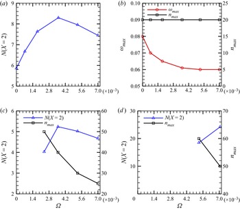
In figure 10(a), we summarise the dependence of the  $N$ factor at
 $X=2$ on
 $\varOmega$ for the travelling MM. It is clearly seen that the MM amplification reaches its peak at
 $\varOmega \approx 0.0036$, corresponding to case IV. As shown in (b), the frequency of the most amplified MM decreases with the increase of
 $\varOmega$, but approaches a constant 0.06 when
 $\varOmega$ is greater than 0.0036. The circumferential wavenumber stays unchanged for all rotation rates considered. Therefore, from the traditional
 $e^N$ transition prediction method, we may conclude that for the travelling-mode-induced transition, the earliest transition occurs when
 $\varOmega \approx 0.0036$. However, things are not that simple. In the following, we will show that the nonlinear effect will lead to a different dependence of the transition onset on
 $\varOmega$. In (c), we plot the dependence on
 $\varOmega$ of the
 $N$-factor accumulation and the circumferential wavenumber of the stationary CFM. Note that the CFM is stable for
 $\varOmega \le 0.0007$. Similar to the results in (a), the
 $N$ factor of the stationary CFM reaches its maximum at
 $\varOmega \approx 0.0036$, but its value is much smaller than that of the MM. The most unstable circumferential wavenumber decreases with
 $\varOmega$. In (d), we plot the dependence of the
 $N$ factor for the CM on
 $\varOmega$. Because the CM is unstable only for cases V and VI, the plot starts from
 $\varOmega =0.0053$. The accumulated
 $N$ factor increases with
 $\varOmega$, and its value is remarkably greater than that for the MM.
(a) Dependence on  $\varOmega$ of the
 $N$ factors at
 $X=2$,
 $N(X=2)$, for the type-I MMs; (b) dependence on
 $\varOmega$ of the most unstable frequency
 $\omega _{max}$ and circumferential wavenumber
 $n_{max}$ for the type-I MMs; (c,d) dependences of
 $N(X=2)$ and
 $n_{max}$ on
 $\varOmega$ for the stationary CFMs and CMs, respectively.

4. Nonlinear evolution of the boundary-layer perturbations
4.1. Parameters for the NPSE calculations
Based on the base flow obtained from § 3.1, we perform the NPSE calculations starting from a streamwise position  $X=1$, which march downstream until their blowup. The streamwise grid spacing is chosen to be
 $dX=0.0043$ (or
 ${\textrm {d}x}=5.07$). In the wall-normal direction, we choose
 $y \in [0,2500]$ (such a large
 $y$-domain is employed to ensure that the attenuation conditions are satisfied in the far field) and 581 non-uniform grid points that are clustered in the near-wall region are employed, for which the coordinate
 $y_j$ at the
 $j^{th}$ point is
 \begin{equation} y_j=\frac{ j /J}{1+(y_{J}/\delta_{99}-2)(1-j/J)} y_J, \quad j \in [0,J], \end{equation}
where  $\delta _{99}=8.7$ denotes the nominal boundary-layer thickness at
 $x=x_0$ and
 $J=580$. Such an allocation ensures that half of the total grid points are allocated to the boundary layer, which has also been used in our previous work (Zhao, Dong & Yang Reference Zhao, Dong and Yang2019; Song et al. Reference Song, Dong and Zhao2022).
From § 3, we know that, for cases I and II, there is only one linear instability mode, the travelling MM; for cases III and IV, the type-I MM and the type-I CFM coexist; for cases V and VI, there are three instability modes, namely, type-I MM, type-I CFM and type-II CM. The type-I CFM is always less unstable than the MM, but the type-II CM, if exists, is much more unstable. In this paper, the NPSE calculations start from a location where the linear instability modes have already been excited, and so a careful selection of the initial perturbations is required. First, we decide to exclude the type-I CFM as the initial perturbation because of its small growth rate. Second, the type-II CM shows a quasi-stationary nature, which is more likely to be excited by either surface imperfections, such as roughness, or the nonlinear interactions between travelling modes. In this paper, we assume the cone to be smooth without any surface imperfection, and so the CM instability is not introduced in the first place. However, for high rotation rates, the nonlinear interaction of the travelling modes can support its initial amplitude, and its high growth rate for strong rotation cases ensures its dominant role in the downstream locations.
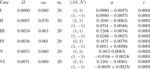
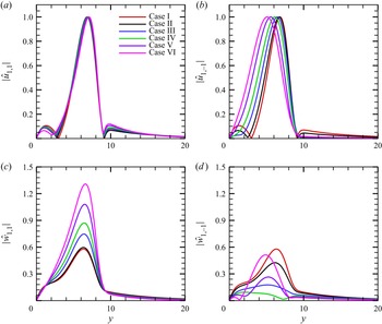
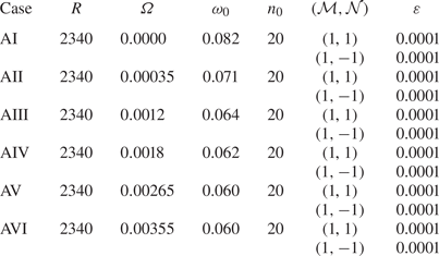
For each of the six rotation rates as studied in § 3.1, we choose the most linearly amplified type-I travelling MM as one of the two initial perturbations, whose frequency and circumference wavenumber can be found in figure 10(a,b), respectively. They are denoted by the fundamental frequency  $\omega _0$ and the fundamental wavenumber
 $n_0$, respectively. In the following, each Fourier component with a frequency
 ${\mathcal {M}} \omega _0$ and a circumference spanwise wavenumber
 ${\mathcal {N}} n_0$ is denoted by (
 ${\mathcal {M}},{\mathcal {N}}$) for convenience, and so the aforementioned introduced mode is denoted by (
 $1,1$). An MM with the same frequency but the opposite circumferential wavenumber, denoted by (
 $1,-1$), is also introduced. The detailed parameters for the two introduced modes are listed in table 3, and the shape functions of
 $\hat u_{1,\pm 1}$ and
 $\hat w_{1,\pm 1}$ are shown in figure 11. Note that the calculations are performed in a moving frame, and are not affected by the rotation. In the NPSE calculations, the nonlinear interaction between the introduced MMs leads to generation of the MFD (
 $0,0$), the streak mode (
 $0,2$), the high-order harmonics (
 $2,0$) and so on. Sketches of the wall pressure in the
 $t$–
 $\varphi$ plane for representative Fourier components,
 $(1,1), (1,-1), (2,0)$ and (
 $0,2$), are shown in figure 12. When the amplitudes of the perturbations have accumulated to sufficiently high levels, the mean flow would undergo such a rapid distortion due to the strong Reynolds stress that the parabolic assumption ceases to be valid. This leads to a blowup of the NPSE calculation. As confirmed by a number of previous direct numerical simulation (DNS) studies (Dong et al. Reference Dong, Zhang and Zhou2008; Zhang & Zhou Reference Zhang and Zhou2008; Mayer et al. Reference Mayer, Fasel, Choudhari and Chang2014), such a blowup phenomenon indicates the onset of laminar–turbulent transition, and the NPSE calculations upstream of the blowup point agree well with the DNS results.
Parameters of the introduced MMs for the NPSE calculations.

Eigenfunctions of the introduced MMs obtained by LST at  $X=1$: (a)
 $|\hat {u}_{1,1}|$; (b)
 $|\hat {u}_{1,-1}|$; (c)
 $|\hat {w}_{1,1}|$; (d)
 $|\hat {w}_{1,-1}|$.

Sketches of the wall pressure in the  $t$–
 $\varphi$ plane for representative Fourier components: (a) (1,1); (b) (
 $1,-1$); (c) (
 $2,0$); (d) (
 $0,2$).

4.2. Cases I and II: OB regime
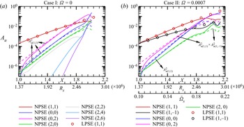
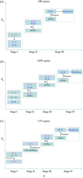
The OB regime usually appears in a quasi-2-D supersonic boundary layer, as for cases I and II in this paper. The solid curves in figure 13 show the evolution of the  $\tilde u$-amplitude of representative Fourier components obtained by NPSE for these two cases. Note that the local Reynolds number
 $R_x$ and the local rotation rate
 $\bar \varOmega _x$ vary with the streamwise location
 $X$, and so they are also marked in the horizontal axis in each panel, where
 \begin{equation} R_x=\frac{\rho^*_e U^*_e x^*}{\mu^*_e},\quad \bar \varOmega_x=\frac{ \varOmega^{*}x^{*} \sin \theta} {U_e^{*}}. \end{equation}
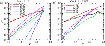
In case I, the amplitude evolution of the fundamental modes ( $1,1$) and (
 $1,-1$) are identical, and so only the former is plotted. We also show the LPSE predictions by the circles for comparison. For each case, the evolution of the fundamental modes
 $(1,\pm 1)$ agrees with the LPSE prediction until
 $X\approx 1.8$, indicating the linear feature of the fundamental modes for the majority of the laminar phase. The growth of the streak mode (
 $0,2$) is mainly attributed to the direct interaction of (
 $1,1$) and (
 $1,-1$). It shows a super-exponential growth in the close neighbourhood of
 $X=1$, followed by a growth rate that is the sum of the fundamental modes
 $(1, \pm 1)$, as confirmed by the pink dashed lines; although its amplitude is preliminarily smaller than those of the fundamental modes, its high growth rate ensures its dominant role in the downstream region. The 2-D travelling component (
 $2,0$), also driven by the direct interaction of
 $(1,\pm 1)$, shows the same growth rate as that of (
 $0,2$) (see the green dashed lines), but its amplitude is not as large as the streak component (
 $0,2$) because of its weaker amplification initially. The MFD is also much weaker than the streak mode in the early laminar phase. For
 $\varOmega =0$ (case I), the extra amplification of the streak mode (
 $0,2$) in the early laminar phase has been explained by an asymptotic theory based on the weakly nonlinear analysis (WNA) in Song et al. (Reference Song, Dong and Zhao2022); the explanation for a non-zero
 $\varOmega$ (case II) is in principle the same, and can be found in Appendix B.
The  $A_u$-evolution of the Fourier components obtained by NPSE for cases I (a) and II (b). The dashed lines denote the theoretical prediction of the growth rate by direct interaction of the introduced oblique modes.

For case I, in the late laminar phase,  $X>1.88$, the harmonics
 $(2,0), (2,2), (2,4)$ and (
 $2,6$) undergo drastic amplification with almost the same growth rate. Because the dominant perturbations in this region are the streak mode (
 $0,2$) and the MFD (
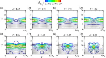
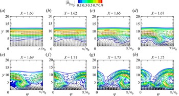
 $0,0$), this phenomenon is a reminiscent of the SI of a streaky profile. In order to confirm the occurrence of the SI of a streaky base flow, we compare the perturbation profiles
 $|{\tilde u}_{2 \omega _{0}}|$ in the
 $y$–
 $\varphi$ plane at different
 $X$ locations for case I in figure 14, where
 \begin{equation} {{\tilde u}_{2{\omega _0}}}\left( {x,y,\varphi } \right) = \int_0^{2{\rm \pi} /{\omega _0}} {\tilde u\left( {x,y,\varphi ,t} \right)\exp \left( { - 2i{\omega _0}} \right){\rm d} t}, \end{equation}
with  $\tilde u$ being obtained by NPSE. The dashed black lines denote the streaky base flow consisting of the laminar base flow, the MFD and the streak components including
 $(0,2), (0,4)$, etc. It can be seen that, as
 $X$ increases, the profile of the unsteady travelling perturbation becomes concentrated around the top of the streak ‘head’, and the perturbation is found to be symmetric about the centre of the streak, showing a varicose feature.
Contours of the perturbation profiles  $|{\tilde u}_{2 \omega _{0}}|$ in the
 $y$–
 $\varphi$ plane for case I. The dashed lines denote the contours of
 $\breve \varPhi _{B}(y,\varphi )$.

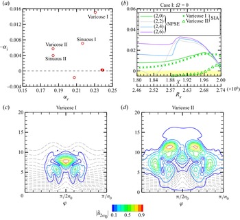
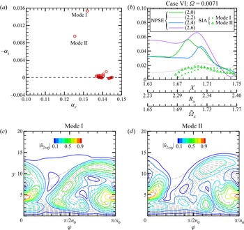
Then, we perform the SIA (introduced in § 2.3.2) based on the streaky base flow obtained by NPSE, and the eigenvalues of the growth rates at  $X=2$ for case I are plotted in figure 15(a). Four dominant unstable modes are found, including two sinuous modes (whose eigenfunctions are anti-symmetric about the centre line) and two varicose modes (whose eigenfunctions are symmetric about the centre line), and the varicose I mode is the most unstable one. The other eigen-solutions with quasi-neutral or stable features are not of our interest, and so are not labelled. Tracing the growth rates of the two varicose modes, as shown by the symbols in (b), we find that the growth rate of the varicose I agrees well with the NPSE results of (
 $2,0$) until
 $X=1.97$, confirming that the dominant mechanism of the growth of this component is the SI of the (
 $0,2$)-induced streaky base flow. However, the higher-order modes,
 $(2,2), (2,4)$ and (
 $2,6$) show greater growth rates than the SIA-predicted growth rate, because these modes are also affected by the nonlinear interaction of (
 $2,0$) with other components. The eigenfunctions of the two varicose modes are shown in figure 15(c,d), respectively, which can well predict the local peaks and the overall shape of the perturbation profile in figure 14(h).
(a) Eigenvalues obtained by SIA for  $\omega =2\omega _{0}$ at
 $X=2$; (b) comparison of the growth rates between SIA and NPSE. (c,d) Eigenfunctions of the varicose I and varicose II modes obtained by SIA, respectively.

For case II, shown in figure 13(b), the nonlinear evolution is quite similar, but the only difference is that the growth rate of the MFD, which is twice the growth rate of ( $1,1$), is not equal to that of the streak mode, which is the sum of the growth rates of (
 $1,1$) and (
 $1,-1$). Because for a rotating cone, where the growth rate of (
 $1,1$) is larger than that of (
 $1,-1$), the MFD grows with a faster rate than the streak mode (
 $0,2$) and the travelling mode (
 $2,0$). Thus, although the amplitude of the MFD is initially smaller than the streak mode, it overwhelms the latter in a downstream position,
 $X=1.96$. It is also predicted that, if
 $\varOmega$ is increased further, the streak-mode-dominated region would shrink and eventually disappear, and so the oblique breakdown regime would be replaced by another regime, as will be introduced in the next subsection.
4.3. Cases III and IV: generalised fundamental resonance (GFR) regime
When  $\varOmega$ is increased to 0.0024 and 0.0036, or
 $\bar \varOmega$ reaches 0.34 and 0.51 (cases III and IV), the growth rates of the two introduced oblique modes are remarkably different, namely, (
 $1,1$) becomes more unstable but (
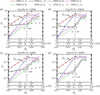
 $1,-1$) becomes almost neutral. This is because the base flow shows a strong asymmetric feature due to the rotation, for which the oblique-breakdown regime as in the quasi-symmetric cases, cases I and II, is not likely to occur. Figure 16(a,c) shows the amplitude evolution of the streamwise and spanwise velocity perturbations for each Fourier component for case III, respectively. The component (
 $1,1$) shows a linear amplification until around
 $X=1.80$, after which it saturates due to the nonlinear effect; the other introduced mode, (
 $1,-1$), shows a much weaker amplification due to its small growth rate before
 $X=1.80$, which is followed by a drastic amplification until reaching the same magnitude as that for (
 $1,1$). Additionally, the evolution of both (
 $1,1$) and (
 $1,-1$) before
 $X=1.8$ agrees well with the linear prediction (LPSE). Before
 $X=1.8$, the MFD grows with a doubled growth rate of that of (
 $1,1$), which ensures that the amplitude of the MFD reaches the same magnitude of (
 $1,1$) in a short distance, leading to the nonlinear saturation of (
 $1,1$). In this region, the growth rates of the streak mode (
 $0,2$) and the harmonic travelling mode (
 $2,0$) are the sum of the growth rates of (
 $1,1$) and (
 $1,-1$), and are smaller than that of the MFD. For case IV, as shown in (b,d), the scenario is the same, but the saturation position of the fundamental oblique mode
 $(1, 1)$ appears earlier. Comparing with cases I and II, we find that an increase of the angular rotation rate
 $\varOmega$ leads to a greater difference between the MFD and the streak mode. As a consequence, for a moderate
 $\varOmega$, the streak mode no longer becomes dominant before the MFD overwhelms (
 $1,1$), and so the OB regime does not appear in cases III and IV. After the saturation of the dominant component (
 $1,1$), the amplitude of the MFD ceases to grow, but the components
 $(0,2), (2,0)$ and (
 $1,-1$) undergo rapid amplifications with almost the same rate, which is attributed to the SI of the saturated (
 $1,1$) component, as will be proven in the following. Being different from the SI of the streaky profiles
 $\breve \varPhi _{B}(y,\varphi )$ discussed in § 4.2, the SI here is supported by a wavy base flow
 $\breve \varPhi _B(\tilde x,y)$.
The amplitude evolution of the Fourier components obtained by NPSE for cases III and IV. (a,c) Case III; (b,d) case IV. (a,b)  $A_u$; (b,d)
 $A_w$. The vertical dashed line in each panel represents the position where (
 $1,1$) saturates.

Actually, the amplification of the streak mode ( $0,2$) may be attributed to a few mechanisms, including (A) the nonlinear interaction of components (
 $1,1$) and (
 $1,-1$), (B) the linear growth of the type-I CFM, (C) the linear growth of the type-II CM and (D) the SI induced by the wavy base flow
 $\breve \varPhi _B(\tilde x,y)$. In order to prescribe the dominant mechanism leading to the streak amplification, we compare the theoretical predictions of the
 $A_u$ evolution of (
 $0,2$) based on these candidates with the NPSE calculations for case IV in figure 17. It is seen that neither of the mechanisms (B) and (C) can reproduce the streak amplification. In the region
 $X<1.78$, the NPSE result agrees with the WNA prediction as introduced in Appendix B, confirming that the growth of the streak mode in the early phase is driven by mechanism (A). This is also the reason why the streak mode (
 $0,2$) shows a greater amplitude than the MFD (
 $0,0$) in the close neighbourhood of
 $X=1$. Performing the SIA introduced in § 2.3.1 based on a wavy base flow consists of the laminar base flow, the MFD, the saturated fundamental mode (1,1) and its harmonics
 $(2,2), (3,3)$, etc., we calculate the amplitude growth of the SI mode for a skewed spanwise wavenumber
 $\breve \beta = -\sin \varTheta \alpha _{r,(0,2)} +\cos \varTheta 2 n_0 /r_0$, as shown by the crosses in figure 17, which is confirmed to agree well with the NPSE calculation for
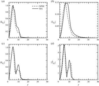
 $X>1.78$. As shown in figure 18, the agreement of the eigenfunctions obtained by SIA and NPSE is also satisfactory, confirming that the late-stage growth of the streak mode is attributed to the mechanism (D).
Comparison of the  $A_u$-evolution for (
 $0,2$) obtained by different approaches for case IV.

Comparison of the eigenfunction of ( $0,2$) obtained by the NPSE and SIA at
 $X=1.9$: (a)
 $|\hat {u}_{0,2}|$; (b)
 $|\hat {v}_{0,2}|$; (c)
 $|\hat {w}_{0,2}|$; (d)
 $|\hat {T}_{0,2}|$.

Such an SI is a reminiscent of the fundamental resonance regime in hypersonic boundary layers, as observed in Sivasubramanian & Fasel (Reference Sivasubramanian and Fasel2015), Chen et al. (Reference Chen, Zhu and Lee2017) and Hader & Fasel (Reference Hader and Fasel2019). In the present study, the introduced fundamental mode ( $1,1$) plays the same role as the 2-D Mack second mode in the 2-D boundary layers in the fundamental resonance regime. It dominates the perturbation field in the early laminar phase, and promotes the growth of the MFD due to its direct interaction with its complex conjugate. When the fundamental mode saturates, its SI encourages the rapid amplification of the streak mode, as well as other travelling waves. Therefore, this regime is referred to as the GFR regime. In the very late stage, as shown in figure 16(a,b), the streak mode becomes the dominant perturbation eventually, supporting the SI modes as for the OB regime. The blowup of the NPSE calculation appears when the mean flow undergoes sufficient distortion forced by the SI modes.
4.4. Cases V and VI: centrifugal-instability-induced transition (CIT) regime
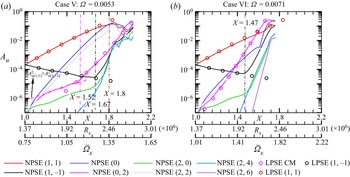
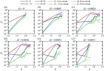
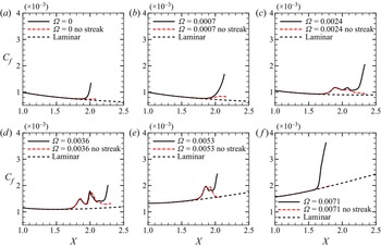
Now we consider the nonlinear evolution of the perturbations for strong rotation rates. The solid curves in figure 19(a) display the  $A_u$-evolution of the representative Fourier components obtained by NPSE for case V. It is seen that the introduced fundamental component (
 $1,1$) amplifies with its linear growth rate until
 $X \approx 1.8$, where it reaches the saturation state with an amplitude of approximately 0.1. The other introduced mode (
 $1,-1$) decays with its linear decay rate until
 $X\approx 1.67$, after which a sharp amplification appears. The streak component (
 $0,2$) also shows a growth rate that is the sum of (
 $1,1$) and (
 $1,-1$) before
 $X \approx 1.52$, confirmed by the pink dashed line in (a), after which a much greater growth rate is observed. Increasing
 $\varOmega$ to
 $0.0071$ or
 $\bar \varOmega$ reaches 1.01, as shown in figure 19(b), the linear growth regions of (
 $1,1$) and (
 $1,-1$) become shorter, and the steak component (
 $0,2$) shows a much greater growth rate than the sum of (
 $1,1$) and (
 $1,-1$) from a position rather close to
 $X=1$. This phenomenon is in contrast to the cases with smaller
 $\varOmega$ values.
The  $A_u$-evolution of the Fourier components obtained by NPSE for cases V (a) and VI (b).

In order to explain the greater growth rate of the ( $0,2$) component, we perform the linear stability analysis of the type-II CM instability by the LPSE approach for these two cases, and compare their accumulated amplitudes with the NPSE results, as shown by the pink circles in figure 19. For case V, the linear growth of the CM can well predict the evolution of (
 $0,2$) when
 $X>1.5$. For case VI, because the CM shows a much greater growth rate, the linear stability analysis yields a good prediction from almost
 $x=x_0$.
For case VI, in the late laminar phase,  $X > 1.7$, the harmonics
 $(2,0), (2,2), (2,4)$ and (
 $2,6$) undergo drastic amplification with almost the same growth rate as shown in figure 19(b). Similar to case I, the dominant perturbations in this region are the streak mode (
 $0,2$) and the MFD (
 $0,0$), and the rapid growths of the harmonics are attributed to the SI of the streaky base flow. However, the difference is that the streak mode (
 $0,2$) is driven by the rapid growth of the CM, instead of the nonlinear interaction between (
 $1,1$) and (
 $1,-1$). In figure 20, we plot the perturbation profiles of
 $|{\tilde u}_{2 \omega _{0}}|$ in the
 $y$–
 $\varphi$ plane at different
 $X$ locations for case VI. The perturbations become localised downstream of
 $X\approx 1.7$, where the streak mode becomes the dominant perturbation.
Contours of the perturbation profiles  $|{\tilde u}_{2 \omega _{0}}|$ in the
 $y$–
 $\varphi$ plane for case VI. The dashed lines denote the contours of
 $\breve \varPhi _{B}(y,\varphi )$.

Performing the SIA for a streaky base flow as introduced in § 2.3.2, we can obtain a set of unstable eigenvalue solutions for  $\omega =2\omega _0$ at
 $X=1.73$, as shown in figure 21(a), where the most unstable two modes are marked mode I and mode II. Tracing the growth rates of the two modes as shown by the symbols in (b), the growth rates of the travelling components
 $(2,0), (2,2), (2,4)$ and (
 $2,6$) obtained by NPSE are compared with the SIA predictions, and favourable agreement is observed in the late phase (
 $X>1.71$), confirming that the rapid amplifications of the travelling modes in this region are attributed to the SI of the streaky base flow. The eigenfunctions of the two modes obtained by SIA are shown in 21(c,d), respectively. Both eigenfunctions can predict the overall shape of the NPSE perturbation profile in figure 20(g).
(a) Eigenvalues obtained by SIA at  $X=1.73$ for
 $\omega =2\omega _{0}$; (b) comparison of the growth rates between SIA and NPSE. (c,d) Eigenfunctions of mode I and mode II obtained by SIA, respectively.

4.5. Summary
In summary, there exist three mechanisms leading to the rapid amplification of the streak component in a supersonic boundary layer over a rotating cone. For small  $\varOmega$ values including
 $\varOmega =0$, the growth of the streak mode is driven by the direct interaction between the introduced fundamental modes (
 $1,1$) and (
 $1,-1$), which can be well explained by the asymptotic analysis based on the WNA. Such a nonlinear process belongs to the OB regime. Increasing
 $\varOmega$ to a moderate level, say
 $\varOmega =0.0036$, the accumulated amplitude of (
 $1,1$) is much greater than that of (
 $1,-1$), and the rapid growth of the streak mode is due to the SI of the saturated travelling mode (
 $1,1$). In the late laminar phase, the streak mode would become the dominant perturbation. Such a nonlinear process belongs to the GFR regime. Further increasing
 $\varOmega$ to 0.0071 or
 $\bar \varOmega = O(1)$, the linear growth rate of the centrifugal instability becomes greater than the amplification due to the aforementioned two regimes, which ensures that the stationary CM (that also shows a stationary streak nature) becomes the dominant perturbation in a short distance. Such a process belongs to the CIT regime.
5. Role of the streak mode in triggering transition
Figure 22 shows the contours of the instantaneous velocity  $u$ in the
 $\varphi$–
 $X$ plane at
 $y/\sqrt {X}=2.25$ for the six cases. In each panel, the high- and low-speed streaks are observed in the late laminar phase, which is parallel to the cone generatrix for
 $\varOmega =0$ but tilts towards the opposite direction of the rotation speed for
 $\varOmega \ne 0$. The inclined angle increases with the increase of the rotation rate. The pink arrow in each panel shows the direction of the streamline at the boundary-layer edge, which agrees overall with the inclined direction of the streaks for each case.
Contours of the instantaneous velocity  $u$ in the
 $X$–
 $\varphi$ plane at
 $y/\sqrt {X}=2.25$. (a–f) Cases I to VI. The pink arrow displays the streamline direction at the boundary-layer edge.

The spiral angle of the streak mode ( $0,2$) for each case can be evaluated by
 \begin{equation} \varPhi = {\left( {{{\tan }^{ - 1}}\frac{{{\alpha _{r,(0,2)}}{r_0}}}{{2{n_0}}}} \right)_{X = {X_b}}}, \end{equation}
where  $\alpha _{r,(0,2)}$ represents its streamwise wavenumber, and
 $2n_0/r_0$ represents its spanwise wavenumber. The measurement is carried out at a location
 $X=X_b$ where the NPSE calculation blows up due to the strong nonlinearity. In figure 23(a), we show its variation on the local rotating rate
 $\bar \varOmega _x$, where the experimental results in Kobayashi et al. (Reference Kobayashi, Kohama, Arai and Ukaku1987) and Tambe et al. (Reference Tambe, Schrijer, Veldhuis and Gangoli2022) are also plotted for comparison. In Kobayashi et al. (Reference Kobayashi, Kohama, Arai and Ukaku1987), the flow is incompressible with the local Reynolds number
 $R_x \sim O(10^4\unicode{x2013} 10^5)$ and the half-apex angle
 $\theta$ ranges from
 $7.5^\circ$ to
 $30^\circ$, whereas in Tambe et al. (Reference Tambe, Schrijer, Veldhuis and Gangoli2022), the Mach number, the local Reynolds number
 $R_x$ and the half-apex angle
 $\theta$ are
 $M\in [0.4,0.6]$,
 $R_x \in [1 \times 10^6, 3\times 10^6]$ and
 $\theta \in [15^\circ,40^\circ ]$, respectively. All the results in (a) almost collapse with the dashed curve, representing the streamline direction of the potential flow,
 $\varPhi _e = \tan ^{-1} \bar \varOmega _x$. The implication is that the spiral angle of the nonlinear structure almost aligns with the direction of the potential flow, irrespective of the Mach number, the Reynolds number and the half-apex angle. Panel (b) shows the dependence on the local rotation rate of the transitional Reynolds number, defined by
 \begin{equation} R_t = \frac{\rho_e^* U_e^* x^*_{b}}{\mu_e^*}, \end{equation}
where  $x_b^*$ represents the dimensional transition location. The experimental results in Kobayashi et al. (Reference Kobayashi, Kohama, Arai and Ukaku1987) and Tambe et al. (Reference Tambe, Schrijer, Veldhuis and Gangoli2022) are also plotted for comparison. Overall, unless the rotation rate is low, the transitional Reynolds number
 $R_t$ decreases with the increase of
 $\bar \varOmega _x$, indicating the significant role of the CM in the CIT transition regime. It needs to be noted that our NPSE calculations do not reflect the exact physical situation because the receptivity process is excluded. Actually, two factors may contribute to the change of
 $R_t$: (i) the initial amplitudes of the introduced MMs should be different; (ii) the CM may also appear as the initial perturbation for strong rotation cases. Thus, it is expected that
 $R_t$ for a higher
 $\bar \varOmega _x$ should be reduced remarkably in reality.
Comparison of the spiral angle of the streaks (a) and the transitional Reynolds number (b) with the literature data.

Since the longitudinal streaks are never absent in the late laminar phase, we may postulate the crucial role of the streaks in triggering transition for all the three regimes. This can be verified by comparing the NPSE results with those obtained by removing artificially the streak component, as shown in figure 24. In the numerical process, the ‘no streak’ curves are calculated by setting the ( $0,2$) components to zero at each streamwise location. In each case, removing the streak component leads to a reduction of the other components in the late laminar phase, and so the blowup of the NPSE calculation disappears or is postponed significantly. Additionally, the streak-impact region is much greater for the GFR and the CIT regimes than that for the OB regime.
Comparison of the  $A_u$-evolution between the NPSE calculations and those by artificially removing the streak component: (a)
 $\varOmega =0.0000$; (b)
 $\varOmega =0.0007$; (c)
 $\varOmega =0.0024$; (d)
 $\varOmega =0.0036$; (e)
 $\varOmega =0.0053$; ( f)
 $\varOmega =0.0071$.

(i) For the OB regime appearing in the low- $\varOmega$ cases, the amplification of the MFD and the travelling mode (
 $2,0$) for the majority of the laminar phase is attributed to the nonlinear interaction of the introduced fundamental modes, while the streak impact only appears when the oblique modes become saturated and the streak mode reaches
 $O(0.1)$ magnitude. The streak-impact region is rather short because the SIA of the streaky profile determines a much higher growth rate of the travelling components, which ensures, in a short distance, their accumulated amplitude to be sufficiently large to distort the mean flow via the Reynolds stress. The latter eventually leads to the sharp rise of the surface friction curve, as will be shown in figure 25(a,b).
Comparison of the  ${C_f}$ curves between the NPSE calculations and those by artificially removing the streak component: (a)
 $\varOmega =0.0000$; (b)
 $\varOmega =0.0007$; (c)
 $\varOmega =0.0024$; (d)
 $\varOmega =0.0036$; (e)
 $\varOmega =0.0053$; ( f)
 $\varOmega =0.0071$.

(ii) For the GFR regime for a moderate  $\varOmega$, the streak impact appears when the fundamental mode (
 $1,1$) and the MFD (
 $0,0$) saturate. Through the SIA for a wavy base flow, it is indicated that the streak mode and a series of travelling modes would also grow. Removing the streak mode artificially would suppress the growth of other travelling modes. Thus, the streak-impact region starts from the saturation of the (
 $1,1$) component. This region is longer than that of the OB regime, because the initial amplitudes of the SI modes are much smaller.
(iii) For the CIT regime in large- $\varOmega$ cases for which
 $\bar \varOmega =O(1)$, the amplification of the streak mode is actually due to the CM instability of the rotating base flow. Since the inflow perturbations do not include the CM, the excitation of the CM instability requires a receptivity process, i.e. the nonlinear interaction of the introduced (
 $1,1$) and (
 $1,-1$) serves as a seed for its initial energy, and its profile adjusts to the CM eigenfunction as it propagates downstream. When the CM amplitude reaches a sufficiently high level, its SI ensures the high growth of the travelling modes, which eventually leads to a remarkable MFD to trigger transition. Such a high growth is not supported if the streak component (CM) is removed.
To demonstrate the impact of the streak mode on the MFD, we compare the streamwise evolution of the coefficients of the skin friction
 \begin{equation} C_f = \left(\frac{{2\bar \mu }}{R}\frac{{\partial \bar u}}{{\partial y}}\right)_{y=0}, \end{equation}
obtained by the original NPSE calculations and those by removing artificially the streak mode, as shown in figure 25, where the overbar represents the temporal and circumferential averaging. For the OB regime ((a) or (b)), the  $C_f$ curve undergoes a sharp increase when the MFD reaches a sufficiently strong level, leading to the blowup of the NPSE calculation. However, when the streak mode is removed, the sharp increase of the
 $C_f$ curve is replaced by a rather mild increase, leading to a postponement of the blowup position. For the GFR regime, shown in (c,d), the
 $C_f$ curves undergo sharp increases three times, and only the third one leads to the blowup of the NPSE calculation. The previous two are related to the saturation and oscillation of the fundamental mode (
 $1,1$), which is not affected by the streak mode. However, since the third increase is attributed to the SI of the streak, removing the streak mode again postpones the blowup position of the NPSE calculation. The multiple increases of the
 $C_f$ curve also exist in the fundamental resonance in hypersonic boundary layers (Sivasubramanian & Fasel Reference Sivasubramanian and Fasel2015; Chen et al. Reference Chen, Zhu and Lee2017; Hader & Fasel Reference Hader and Fasel2019). For the CIT regime, shown in (e, f), the streak mode is the key factor to support the SI. Therefore, the
 $C_f$ curve recover to the laminar state when the streak mode is removed.
6. Effect of the rotation rates on transition
To demonstrate the impact of the rotation rate on the transition location, we normalise the  $C_f$ curves by the laminar skin friction coefficient
 $C_{f0}$, namely,
 $\overline {C_f}=C_f/C_{f0}$, as shown in figure 26(a). For the OB and CIT regimes, the
 $\bar C_f$ curve only undergoes a sharp increase once. However, for the GFR regime, the
 $\bar C_f$ curve increases more than once, and so, different thresholds for the transition onset may lead to different outcomes. Thus, we introduce
 $X_i$ and
 $X_t$ such that
 \begin{equation} {\overline{C_f}}(X_i)=1.05, \quad {\overline{C_f}} (X_t)=1.5.\end{equation}
Admittedly, the choices of these thresholds are a bit artificial, but if we choose  ${\overline {C_f}}(X_i)=1.1$ and
 ${\overline {C_f}}(X_t)=1.6$, then the values of
 $X_i$ and
 $X_t$ vary only 1.63 % and 0.88 % , respectively. Both thresholds are displayed in (a). The dependence of the two locations on the rotation rate
 $\varOmega$ is summarised in figure 26(b). For the OB regime, the locations of
 $X_i$ and
 $X_t$ are quite close, and increase of
 $\varOmega$ does not lead to an apparent change of the transition onset. For the CIT regime, premature transition is observed for a higher rotation rate. For the GFR regime, the first increase of the
 $\overline {C_f}$ curve (
 $X_i$) is much earlier than that of the OB regime and the CIT regime with relatively low
 $\varOmega$, but the last increase (
 $X_t$) is remarkably postponed. Since the transition onset of the GFR regime is related to the last increase, it is readily asserted that, for a moderate
 $\varOmega$, the transition appears later.
(a) Normalised skin friction coefficients  $\bar C_{f}$, where the black dashed and dot-dashed lines denote
 $\bar C_{f}=1.05$ and
 $\bar C_{f}=1.5$, respectively. (b) Dependence on
 $\varOmega$ of
 $X_i$ (where
 $\bar C_{f}=1.05$) and
 $X_t$ (where
 $\bar C_{f}=1.5$).

To this end, two conclusions are drawn. First, for a low- $M$ supersonic boundary layer over a cone, increase of the rotation rate to a moderate level could postpone the transition onset, which is favourable for the reduction of the total drag for flying vehicles. Second, considering the different nonlinear transition regimes, the transition prediction based on the linear instability analysis, i.e. the
 $e^N$ method, should be carefully used. From the linear prediction as in figure 10, it is seen that the introduced fundamental mode undergoes the greatest amplification when the rotation rate is moderate. Therefore, from the traditional
 $e^N$ method we may conclude that the transition is promoted at this rotation rate. However, it is seen from the NPSE calculations that such a conclusion is completely wrong, which is attributed to the nonlinear regimes appearing for different
 $\varOmega$ values.
7. Effect of the initial position on NPSE calculations
Since the above NPSE calculations are all started from the same streamwise position  $x_0^*=137$ mm that is arbitrarily chosen, one may query the impact of the initial position on the nonlinear transition regimes. Therefore, in this section, we choose another
 $x_0^*$, namely,
 $x_0^*=548$ mm, to perform the NPSE calculations with the other conditions unchanged, and make comparison with the previously obtained nonlinear regimes.
From (2.1a), it is calculated that, for  $x_0^*=548$ mm, the Reynolds number
 $R=2340$, which is twice that in table 1. To fix the initial rotation rate
 $\bar \varOmega$ for the six case studies, the angular velocity
 $\varOmega$, according to (2.3), is half of that in table 2 for each case. From the linear instability analysis, the parameters of the introduced perturbations are shown in table 4. Here, the frequency of the introduced MM instabilities for each case changes slightly in comparison with that in table 2, but the fundamental circumferential wavenumber
 $n$ stays the same.
Parameters of the introduced MMs for the NPSE calculations.

Skipping the numerical details, we directly show the normalised skin friction coefficient  $\bar C_f$ in figure 27(a). Compared with figure 26(a), we find that the sharp increase of the
 $\bar C_f$ curve, representing the strong distortion of the mean flow, appears at a smaller
 $X$ value for each case, due to the more unstable nature for a greater Reynolds number. However, the transitional Reynolds number is greater in figure 27(a), which is because the initial position
 $x_0^*$ of the NPSE calculation is four times greater than that in figure 26(a). Nonetheless, the overall trend of
 $\bar C_f$ curves in the two figures are rather close, which can be clearly demonstrated by summarising the dependence of
 $X_i$ and
 $X_t$ shown in figure 27(b). The effect of the three nonlinear regimes agrees qualitatively with those in figure 26(b), indicating that an arbitrarily chosen initial position is adequate for the purpose of the present study.
(a) Normalised skin friction coefficients  $\bar C_{f}$, where the black dashed and dot-dashed lines denote
 $\bar C_{f}=1.05$ and
 $\bar C_{f}=1.5$, respectively. (b) Dependence on
 $\varOmega$ of
 $X_i$ (where
 $\bar C_{f}=1.05$) and
 $X_t$ (where
 $\bar C_{f}=1.5$).

8. Concluding remarks and discussion
In this paper, the effect of cone rotation on the nonlinear evolution of travelling MMs in a Mach-3 supersonic boundary layer over a  $7^{\circ }$-semi-apex-angle rotating cone is studied. The linear instability analysis shows that the most linearly amplified travelling MMs appear when the circumferential wavenumber
 $n\approx 20$, and their frequencies decay with the increase of
 $\varOmega$. These modes, marked by (1,1), together with their counterparts (
 $1,-1$), are introduced as the initial perturbations for the NPSE calculations, and three distinguished regimes, namely, the OB regime, the GFR regime and the CIT regime, appear sequentially from low to high
 $\varOmega$ values.
For a small  $\varOmega$ value, the boundary-layer transition is most likely to be triggered by the OB regime, as sketched in figure 28(a). In the early stage (stage I), the introduced two oblique modes amplify with their linear growth rates, and their interaction leads to the amplifications of the streak component (
 $0,2$) and the travelling-wave component (
 $2,0$) with a growth rate being the sum of those of (
 $1,1$) and (
 $1,-1$). The streak mode undergoes an extra amplification, showing a much greater amplitude than (
 $2,0$), as well as other components. This phenomenon can be explained by the asymptotic analysis in Song et al. (Reference Song, Dong and Zhao2022) or in Appendix B of this paper. In stage II, the streak mode becomes the dominant perturbation, which, together with the MFD, supports the rapid amplification of the harmonic travelling waves (HTWs) due to the SI regime. When the latter have accumulated to finite amplitudes (stage III), they can promote a rapid distortion of the mean flow by producing sufficient Reynolds stress, leading to a sharp increase of the surface friction coefficient and the transition onset.
Schematics of the OB (a), GFR (b) and CIT (c) regimes, where HTW stands for harmonic travelling wave.

For a moderate  $\varOmega$, the component (
 $1,1$) shows a greater linear growth rate, while the component (
 $1,-1$) is stabilised. When the dominant mode (
 $1,1$) saturates, the SI regime supports the rapid amplification of other Fourier components, including the streak mode (
 $0,2$) and the travelling waves such as (
 $1,-1$). In a skewed moving frame with the same direction of (
 $1,1$), such a regime is the same as the fundamental resonance in principle, i.e. the saturated oblique mode (
 $1,1$) plays the same role as the saturated 2-D travelling mode as marked by the yellow circle in figure 1(b), and the SI modes (
 $0,2$) and (
 $1,-1$) act as the fundamental resonance modes as marked by the grey circles in figure 1(b). Remarkably, the consequence of this SI would eventually ensure the dominant role of the streak mode (0, 2), which further encourages the SI of a streaky base flow. This repeats the stage III of the OB regime, and leads to the transition onset. The process is sketched in figure 28(b).
For a large  $\varOmega$ value such that
 $\bar \varOmega =O(1)$, shown in figure 28(c), the streak mode (
 $0,2$), originally generated by the direct interaction of (
 $1,1$) and (
 $1,-1$), undergoes a rapid amplification due to the centrifugal-induced instability. This amplification is indeed a linear regime, in contrast to the aforementioned two regimes. When the linear CM has accumulated to a finite amplitude, the mean flow would show a streaky feature, which supports the high growth rate of the SI modes (HTWs). Again, since these modes produce sufficient MFD via the Reynolds stress, the breakdown of the laminar flow would appear eventually.
Comparing the transition processes as sketched in figure 28, we find that the last two stages of each regime show the same scenario, namely, the rapidly amplified HTWs, supported by the SI of the streaky base flow, promote sufficient MFD to trigger transition. Remarkably, the streak mode plays a crucial role in the transition process, and if the streak mode is removed artificially, the transition location would be severely postponed or disappear, as shown in figure 25.
Remarkably, since different nonlinear transition regimes appear for the different rotation rates, the traditional transition-prediction approach by only considering the linear instability may be insufficient. For the present configuration, as shown in figure 10, the accumulated amplitude due to the linear instability reaches its maximum when  $\varOmega \approx 0.0036$. On the contrary, the NPSE calculations show that the transition induced by the OB regime (low
 $\varOmega$) and CIT regime (large
 $\varOmega$ such that
 $\bar \varOmega =O(1)$) could be much earlier. The main reason is that, for
 $\varOmega \approx 0.0036$, the GFR regime appears, for which the
 $C_f$ curve undergoes sharp increases more than once. The linear prediction usually predicts the first sharp increase of the
 $C_f$ curve, which, however, does not indicate the breakdown of the laminar flow. Therefore, the transition-prediction method based on the linear instability analysis should be carefully used if multiple nonlinear breakdown regimes may appear.
Funding
This work is supported by National Science Foundation of China (Grant Nos. 11988102, U20B2003, 12002235) and Strategic Priority Research Program, CAS (No. XDB22040104).
Declaration of interests
The authors report no conflict of interest.
Appendix A. Matrices and nonlinear terms in disturbance equation
In (2.10),  ${ \boldsymbol {G} }$,
 $\boldsymbol {A}$,
 $\boldsymbol {B}$,
 $\boldsymbol {C}$,
 $\boldsymbol {D}$,
 ${\boldsymbol {V}}_{xx}$,
 ${\boldsymbol {V}}_{yy}$,
 ${\boldsymbol {V}}_{\varphi \varphi }$,
 ${\boldsymbol {V}}_{xy}$,
 ${\boldsymbol {V}}_{y \varphi }$ and
 ${\boldsymbol {V}}_{x \varphi }$ are
 $5 \times 5$-order matrices. Most of the non-zero elements are the same as those in the appendix A of Song et al. (Reference Song, Dong and Zhao2022), and here we only present the ones with different expressions
 \begin{gather} \left.\begin{gathered}
{A_{45}} = \frac{{ - 2\tau {S_{B,13}}}}{R},\quad {A_{54}}
={-} \frac{{4\left( {\gamma - 1}\right){M^2}}}{R}{\mu
_B}{S_{B,13}},\quad {B_{45}} = \frac{{ - 2\tau
{S_{B,23}}}}{R},\\ {B_{54}} ={-} \frac{{4\left( {\gamma -
1} \right){M^2}}}{R}{\mu _B}{S_{B,23}},\quad {C_{11}} =
\frac{{{W_B}}}{r},\quad {C_{22}} = \frac{{{\rho
_B}{W_B}}}{r},\\ {C_{25}} = \frac{{ - 2\tau
{S_{B,31}}}}{rR},\quad {C_{33}} = \frac{{{\rho
_B}{W_B}}}{r},\quad {C_{35}} = \frac{{ - 2\tau
{S_{B,32}}}}{{r{{\rm R}}}},\quad {C_{44}} = \frac{{{\rho
_B}{W_B}}}{r},\\ {C_{51}} ={-} \frac{{\gamma - 1}}{{r\gamma
}}{T_B}{W_B},\quad {C_{52}} ={-} \frac{{4\left( {\gamma -
1} \right){M^2}}}{rR}{\mu _B}{S_{B,31}},\\ {C_{53}} ={-}
\frac{{4\left( {\gamma - 1} \right){M^2}}}{rR}{\mu
_B}{S_{B,32}},\quad {C_{55}} = \frac{{{\rho
_B}{W_B}}}{{r\gamma }},\\ {D_{21}} = ( {{U_B}{U_{B,x}}
+ {\tilde V_B}{U_{B,y}} - g\overset{\frown}{W} _B^2}) + \frac{{{T_{B,x}}}}{{\gamma {M^2}}},\quad {D_{24}} ={-} 2g{\rho _B}{{\overset{\frown}{W}}_B},\\
{D_{31}} = ({{U_B}{\tilde V_{B,x}} + {\tilde
V_B}{\tilde V_{B,y}} - h\overset{\frown}{W} _B^2}) +
\frac{{{T_{B,y}}}}{{\gamma {M^2}}},\quad {D_{34}} ={-}
2h{\rho _B}{{\overset{\frown}{W}}_B},\\ {D_{41}} =
{U_B}{{\overset{\frown}{W}}_{B,x}} + {\tilde V_B}
{{\overset{\frown}{W}}_{B,y}} +
g{U_B}{{\overset{\frown}{W}}_B} + h{\tilde
V_B}{{\overset{\frown}{W} }_B},\\ {D_{42}} = {\rho
_B}( {{{\overset{\frown}{W}}_{B,x}} +
g{{\overset{\frown}{W} }_B}}),\quad {D_{43}} = {\rho
_B}({{{\overset{\frown}{W}}_{B,y}} +
h{{\overset{\frown}{W}}_B}}),\\ {D_{45}} ={-}
\frac{1}{R}\left\{ \tau [(2{S_{B,13}})_{x} +
(2{S_{B,23}})_{y} + 4h{S_{B,23}} + 4g{S_{B,13}}]{ +
2{S_{B,13}}{\tau _x} + 2{S_{B,23}}{\tau _y}} \right\}, \\
{D_{54}} = \frac{{4\mu ( {\gamma - 1}){M^2}}}{R}( {g{S_{B,13}} + h{S_{B,23}}}). \end{gathered}\right\}
\end{gather}
In the above expressions, we have put  $\tilde V_B =R^{-1} V_B$,
 $\tau = {\textrm {d} \mu _B}/{\textrm {d} T_{B}}$,
 ${{\overset {\frown }{W} }_B} = {W_B} + \varOmega r$,
 $g= \sin \theta /r$,
 $h= \cos \theta /r$. Here,
 $\boldsymbol {S_B}$ denotes the rate of strain tensor of the base flow, whose components are
 \begin{equation} \left.\begin{gathered}
{S_{B,11}} = {U_{B,x}},\quad {S_{B,22}} = {\tilde
V_{B,y}},\quad {S_{B,33}} = g{U_B} + h{\tilde V_B},\\
{S_{B,12}} ={S_{B,21}} =( {{\tilde V_{B,x}} + {U_{B,y}}})/2,\\ {S_{B,13}}={S_{B,31}} =
( {{W_{B,x}} - g{W_B}} )/2,\quad {S_{B,23}}
={S_{B,32}}= ( {{W_{B,y}} - h{W_B}})/2.
\end{gathered}\right\} \end{equation}
The nonlinear forcing  ${\boldsymbol {F}}= [F^{(1)},F^{(2)},F^{(3)},F^{(4)},F^{(5)} ]^{\textrm {T}}$, with
 \begin{align} \left.\begin{aligned}
{F^{(1)}} &={-} \left( {\tilde \rho \boldsymbol{\nabla}
\boldsymbol{\cdot} {\boldsymbol{u}} + {\boldsymbol{u}}
\boldsymbol{\cdot} \boldsymbol{\nabla} \tilde \rho }
\right), \\ {F^{(2)}} &={-} \tilde \rho {{\tilde u}_t} -
\tilde \rho ( {{U_B}{{\tilde u}_x} + {\tilde
V_B}{{\tilde u}_y} + {{{W_B}{{\tilde u}_\varphi }}/ r} +
\tilde u{U_{B,x}} + \tilde v{U_{B,x}} -
2g{{\overset{\frown}{W} }_B}\tilde w}) \\ &\quad
-( {\tilde \rho + {\rho _B}} ) ( {\tilde
u{{\tilde u}_x} + \tilde v{{\tilde u}_y} + {{\tilde
w{{\tilde u}_\varphi }}/{r - g{{\tilde w}^2}}}}) -
\frac{{{{( {\tilde \rho \tilde T} )}_x}}}{{\gamma {M^2}}} -
\frac{2}{{3R}}{( {\tilde \mu \boldsymbol{\nabla}
\boldsymbol{\cdot} {\boldsymbol{u}}})_x} \\ &\quad +
\frac{2}{R} [ {{{( {\tilde \mu {{\tilde S}_{11}}})}_x} + {{( {\tilde \mu {{\tilde S}_{21}}}
)}_y} + {{{{( {\tilde \mu {{\tilde S}_{31}}})}_\varphi }}/r} + \tilde \mu ( {g{{\tilde
S}_{11}} + h{{\tilde S}_{21}} - g{{\tilde S}_{33}}}
)}], \\ {F^{(3)}} &={-} \tilde \rho {{\tilde
v}_t} - \tilde \rho ( {{U_B}{{\tilde v}_x} + {\tilde
V_B}{{\tilde v}_y} + {W_B}{{{{\tilde v}_\varphi }}/r} +
\tilde u{\tilde V_{B,x}} + \tilde v{\tilde V_{B,y}} -
2h\overset{\frown}{W} \tilde w})\\ &\quad - \left(
{\tilde \rho + {\rho _B}} \right)( {\tilde u{{\tilde
v}_x} + \tilde v{{\tilde v}_y} + {{\tilde w{{\tilde
v}_\varphi }}/r} - h{{\tilde w}^2}_3}) - \frac{{{{(
{\tilde \rho \tilde T} )}_y}}}{{\gamma {M^2}}} -
\frac{2}{3R}{({\tilde \mu \boldsymbol{\nabla}
\boldsymbol{\cdot} {\boldsymbol{u}}} )_y}\\ &\quad +
\frac{2}{R}[ {{{( {\tilde \mu {{\tilde S}_{12}}})}_x} + {{( {\tilde \mu {{\tilde S}_{22}}} )}_y}
+ {{{{( {\tilde \mu {{\tilde S}_{32}}}
)}_\varphi }} / r} + \tilde \mu ( {g{{\tilde
S}_{12}} + h{{\tilde S}_{22}} - h{{\tilde S}_{32}}}
)} ] ,\\ {F^{(4)}} &={-} \tilde \rho {{\tilde
w}_t} - \tilde \rho [ {{U_B}{{\tilde w}_x} + {\tilde
V_B}{{\tilde w}_y} + \tilde u{{\overset{\frown}{W} }_{B,x}}
+\tilde v{{\overset{\frown}{W} }_{B,y}} + g(
{{{\overset{\frown}{W} }_B}\tilde u + \tilde w{U_B}}
)}\\ &\quad { + {{{W_B}{{\tilde w}_\varphi }} / r}+ h( {{{\overset{\frown}{W}
}_B}\tilde v + \tilde w{V_B}})}] - \frac{{{{(
{\tilde \rho \tilde T} )}_\varphi }}}{{\gamma r{M^2}}}-
\frac{2}{{3rR}}{\left( {\tilde \mu \boldsymbol{\nabla}
\boldsymbol{\cdot} {\boldsymbol{u}}} \right)_\varphi }\\
&\quad - \left( {\tilde \rho + {\rho _B}} \right)\left(
{\tilde u{{\tilde w}_x} + \tilde v{{\tilde w}_y} + {{\tilde
w{{\tilde w}_\varphi }} / r} + g\tilde u\tilde w + h\tilde
v\tilde w} \right) \\ &\quad + \frac{2}{R}[ {{{(
{\tilde \mu {{\tilde S}_{13}}} )}_x} + {{(
{\tilde \mu {{\tilde S}_{23}}} )}_y} + {{{{(
{\tilde \mu {{\tilde S}_{33}}} )}_\varphi }} / r} +
2\tilde \mu ( {g{{\tilde S}_{13}} + h{{\tilde
S}_{23}}} )} ], \\ {F^{(5)}} &={-} \frac{{\tilde
\rho }}{\gamma }( {{{\tilde T}_t} + {\boldsymbol{u}}
\boldsymbol{\cdot} \boldsymbol{\nabla} {T_B} +
{\boldsymbol{U}} \boldsymbol{\cdot} \boldsymbol{\nabla}
\tilde T + {\boldsymbol{u}} \boldsymbol{\cdot}
\boldsymbol{\nabla} \tilde T} ) - \frac{{{\rho
_B}}}{\gamma }( {{\boldsymbol{u}} \boldsymbol{\cdot}
\boldsymbol{\nabla} \tilde T} )+ \boldsymbol{\nabla}
\boldsymbol{\cdot} ( {\tilde \mu \boldsymbol{\nabla}
\tilde T} )\\ &\quad +\frac{{\gamma - 1}}{\gamma
}\tilde T\left( {{{\tilde \rho }_t} + {\boldsymbol{u}}
\boldsymbol{\cdot} \boldsymbol{\nabla} {\rho _B} +
{\boldsymbol{U}} \boldsymbol{\cdot} \boldsymbol{\nabla}
\tilde \rho + {\boldsymbol{u}} \boldsymbol{\cdot}
\boldsymbol{\nabla} \tilde \rho } \right) + \frac{{\gamma -
1}}{\gamma }{T_B}\left( {{\boldsymbol{u}}
\boldsymbol{\cdot} \boldsymbol{\nabla} \tilde \rho }
\right) \\ &\quad + \left( {\gamma - 1} \right){M^2}\left[
{2{\mu _B}{\boldsymbol{\tilde S}}:{\boldsymbol{\tilde S}} -
\frac{2}{3}{\mu _B}{{\left( {\boldsymbol{\nabla}
\boldsymbol{\cdot} {\boldsymbol{u}}} \right)}^2} + 4\tilde
\mu {\boldsymbol{ S_B}}:{\boldsymbol{\tilde S}} -
\frac{4}{3}\tilde \mu \left( {\boldsymbol{\nabla}
\boldsymbol{\cdot} {\boldsymbol{U}}} \right) \left(
{\boldsymbol{\nabla} \boldsymbol{\cdot} {\boldsymbol{u}}}
\right)} \right] \\ &\quad + \left( {\gamma - 1}
\right){M^2}\left\{ {2\tilde\mu {\boldsymbol{\tilde
S}}:{\boldsymbol{\tilde S}} - \frac{2}{3} \tilde \mu
{{\left( {\boldsymbol{\nabla} \boldsymbol{\cdot}
{\boldsymbol{u}}} \right)}^2}} \right\}.
\end{aligned}\right\} \end{align}
In the above expressions,  ${\boldsymbol {U}} = {[ {{U_B},\ {\tilde V_B},\ {W_B}} ]^\textrm {T}}$,
 ${\boldsymbol {u}} = {[ {\tilde u,\tilde v,\tilde w} ]^\textrm {T}}$,
 $\boldsymbol {\nabla } \boldsymbol {\cdot } {\boldsymbol {U}} = {U_{B,x}} + {\tilde V_{B,y}} + g{U_B} + h{\tilde V_B}$,
 $\boldsymbol {\nabla } \boldsymbol {\cdot } {\boldsymbol {u}} = ( {{{\tilde u}_x} + {{\tilde v}_y} + {{{{\tilde w}_\varphi }} / {r + g\tilde u + h\tilde v}}} )$ and
 $\tilde {\boldsymbol {S}}$ denotes the rate of strain tensor of disturbance, whose six independent components are
 \begin{equation} \left.\begin{gathered}
{\tilde S_{11}} = {\tilde u_{x}},\quad {\tilde S_{22}} =
{\tilde v_{y}},\quad {\tilde S_{33}} = {{{{\tilde
w}_\varphi }} / r} + g{\tilde u} + h{\tilde v},\quad
{\tilde S_{12}} ={\tilde S_{21}} = ({{\tilde v_{x}} +
{\tilde u_{y}}})/2,\\ {\tilde S_{13}}={\tilde
S_{31}} = ( {{\tilde w_{x}} + {{{{\tilde u}_\varphi }}
/ r} - g{\tilde w}} )/2, {\tilde S_{23}} ={\tilde
S_{32}}= ({{\tilde w_{y}}+{{{{\tilde v}_\varphi }} /
r} - h{\tilde w}})/2. \end{gathered}\right\}
\end{equation}
Appendix B. Explanation of the extra amplification of the streak mode for a small rotation rate
To explain the extra amplification of the streak mode, we perform the WNA to probe the evolution of the streak mode ( $0,2$) driven by the direct interaction between (
 $1,1$) and (
 $1,-1$)
 \begin{equation} {\varepsilon_{1,1}\varepsilon_{1,-1}}\breve \phi_3(y; X)\exp \left[\text{i} \int \alpha_3 (x) \,{{\rm d}x}+ \text{i} 2n_0 \varphi \right]+O(\varepsilon_{1,1}^2, \varepsilon_{1,-1}^2,\varepsilon_{1,1}\varepsilon_{1,-1}) +\text{c.c.}, \end{equation}
where  $\breve {\phi }_3$ represents the shape function of the streak mode and
 $\alpha _3 \equiv \alpha _{3r}+ \textrm {i} \alpha _{3i} = (\alpha _{1,1}-\alpha _{1,-1})_{r} + \textrm {i} (\alpha _{1,1}+\alpha _{1,-1})_{i}$. Note that, for an unstable MM, we have
 $-\alpha _{1i}\ll \alpha _{1r}=O(1)$, and thus
 $\sigma =- \alpha _{3i} \ll 1$ is introduced. In the high-
 $R$ approximation, the inviscid MMs show a double-deck structure, namely, a main layer where
 $y=O(1)$ and a viscous Stokes layer where
 $y=O(R^{-1/2})$ (Dong et al. Reference Dong, Liu and Wu2020; Dong & Zhao Reference Dong and Zhao2021). For the present configuration, the stokes layer is passive, and so we only focus on the evolution in the main layer. Substituting (2.18) and (B1) into the system (2.10) and collecting the
 $O(\varepsilon _{1,1}\varepsilon _{1,-1})$ terms, we obtain
 $$\begin{gather} (\sigma U_B + \text{i} \tilde \alpha \tilde U) M^{2} \breve p_3+ (\text{i} \alpha_{3r} + \sigma) \breve u_3+\breve v_{3,y}+\text{i}\beta_3 \breve w_3 ={{\hat F}_{3}^{(1)}}, \end{gather}$$
 $$\begin{gather}\rho_B[(\sigma U_B + \text{i} \tilde \alpha \tilde U )\breve u_3+U_B'\breve v_3]+ (\text{i} \alpha_{3r} + \sigma) \breve p_3 = {{\hat F}_{3}^{(2)}}, \end{gather}$$
 $$\begin{gather}\rho_B(\sigma U_B + \text{i} \tilde \alpha \tilde U)\breve v_3+ \breve p_{3,y} = {{\hat F}_{3}^{(3)}}, \end{gather}$$
 $$\begin{gather}\rho_B[(\sigma U_B + \text{i} \tilde \alpha \tilde U )\breve w_3+W_B'\breve v_3 ]+\text{i} \beta_3 \breve p_3 ={{\hat F}_{3}^{(4)}}, \end{gather}$$
where  $\beta _3=2n_0/r_0$,
 $\tilde \alpha = \sqrt {\alpha _{3r}^{2}+\beta _{3}^{2}}$,
 $\tilde U = U_{B} \cos \varPhi + W_{B} \sin \varPhi$ (with
 $\varPhi =\tan ^{-1}(\beta _{3}/\alpha _{3r})$ denoting the wave angle). Here,
 $\hat F_3^{(1)}$,
 $\hat F_3^{(2)}$,
 $\hat F_3^{(3)}$ and
 $\hat F_3^{(4)}$ are
 $O(1)$, and can be easily deduced from (A3).
For convenience, we introduce  $\tilde w_3 = \breve u_3 \cos \varPhi + \breve w_3 \sin \varPhi$ and
 $\tilde u_3 = \breve u_3 \sin \varPhi - \breve w_3 \cos \varPhi$. Actually,
 $\tilde U$ represents the base-flow velocity along the wave angle, which is numerically small for inviscid modes, as confirmed by Song & Dong (Reference Song and Dong2023). We assume
 $\tilde U \sim \sigma$, and introduce
 $\tilde U_{1}= \tilde U / \sigma =O(1)$. Then, from a scaling estimate, we obtain
 $\tilde u_3 \sim 1/\sigma ^{2}$,
 $\breve v_{3} \sim \tilde w_{3} \sim 1/\sigma$ and
 $\breve p_{3} \sim 1$. Thus, we introduce
 \begin{equation} \bar u_{3}=\sigma^{2} \tilde u_{3}, \quad ({\bar v}_3, \bar w_{3})=\sigma (\breve v_{3},\tilde w_{3}), \end{equation}
and the system (B2), neglecting the  $O(\sigma )$ terms, can be rewritten as
 $$\begin{gather} \sin \varPhi \bar u_3+\bar v_{3,y}+\text{i} \tilde \alpha \bar w_3 =0, \end{gather}$$
 $$\begin{gather}(\text{i} \tilde \alpha \tilde U_1+ U_B) \bar u_3 + \tilde W_{y} \bar v_3 = 0, \end{gather}$$
 $$\begin{gather}\rho_B(\text{i} \tilde \alpha \tilde U_1 + U_B )\bar v_3+ \breve p_{3,y} = {{\hat F}_{3}^{(3)}}, \end{gather}$$
 $$\begin{gather}\rho_B[(\text{i} \tilde \alpha \tilde U_1 + U_B)\bar w_3 + \tilde U_{1,y} \bar v_3]+ \text{i} \tilde \alpha \breve p_3 = {{\hat F}_{3}^{(2)}} \cos \varPhi + {{\hat F}_{3}^{(4)}} \sin \varPhi, \end{gather}$$
with  $\tilde W = U_B \sin \varPhi - W_B \cos \varPhi$ denoting the velocity perpendicular to the wave-vector direction. Eliminating
 $\bar u_{3}$ and
 $\bar w_3$ from (B4), we arrive at a second-order differential equation system
 $$\begin{gather} \bar v_{3,y}=\frac{\sin \varPhi\tilde W_{y} + \text{i} \tilde \alpha \tilde U_{1,y}}{\text{i} \tilde \alpha \tilde U_1 + U_B }\bar v_3 + \frac{(\text{i} \tilde \alpha)^{2}}{\rho_{B} (\text{i} \tilde \alpha \tilde U_1 + U_B )} \breve p_3 -\text{i} \tilde \alpha \frac{ {{\hat F}_{3}^{(2)}} \cos \varPhi + {{\hat F}_{3}^{(4)}} \sin \varPhi}{\rho_{B} (\text{i} \tilde \alpha \tilde U_1 + U_B ) }, \end{gather}$$
 $$\begin{gather}\breve p_{3,y} ={-}\rho_{B} (\text{i} \tilde \alpha \tilde U_1 + U_B )\bar v_3+{{\hat F}_{3}^{(3)}}, \end{gather}$$
and the boundary conditions read
 \begin{equation} \bar{v}_{3} = 0 \quad \text{at}\ y=0;\quad \breve{p}_{3} \to 0 \quad \text{as}\ y \to \infty. \end{equation}
It is indicated from the above analysis that the key factor causing the extra amplification of the streak mode is the small growth rate of the fundamental mode (of  $O(\sigma )$). The
 $O(\sigma ^{-1})$
 $\breve v_3$ and
 $\breve w_3$ velocities behave like a roll, which are driven by the nonlinear interaction of
 $(1,1)$ and
 $(1,-1)$, whereas the streak component
 $\breve u_3$ is driven by the linear lift-up mechanism, as indicated by (B4b). Thus, the extra amplification of
 $\breve u_3$ leads to the appearance of the longitudinal streaks.
In figure 29(a,b), we compare the perturbation evolution of the ( $0,2$) component between NPSE and WNA for cases I and II, respectively. Good agreement is observed for all the velocity components before the streak mode saturates.
Comparison of the amplitudes of ( $0,2$) components between NPSE and WNA. (a) Case I; (b) case II.

Appendix C. Resolution study for NPSE
In order to confirm the sufficiency of the Fourier-series truncation for the NPSE calculations, we choose cases I and II, and compare the numerical results for  $(M_e, N_e)=(16,32)$ and (
 $8,16$), as shown in figure 30. The two families of curves overlap precisely, confirming the accuracy of our NPSE calculations.
Comparison of NPSE results by different orders of the Fourier-series truncation. Solid lines:  $(M_e, N_e)=(8,16)$; circles:
 $(M_e, N_e)=(16,32)$.

Appendix D. Validation of the SIA for a wavy base flow
In order to verify our SIA code, we repeat the cases of Ng & Erlebacher (Reference Ng and Erlebacher1992) for the subharmonic resonance regime and Xu et al. (Reference Xu, Liu, Mughal, Yu and Bai2020) for the fundamental resonance regime. In each case, the physical model is an adiabatic flat-plate boundary layer with  $M=4.5$ and
 $R_{d}=10\,000$ and
 $T_{e} =61.11K$, where
 $R_d$ is the Reynolds number based on the displacement thickness of the local boundary layer. The base flow is a superposition of the Blasius similarity solution and a saturated 2-D Mack second mode (
 $\alpha _r = 2.52$) with different amplitude
 $\varepsilon$. In each calculation, we choose
 $(M_w,N_w)=(3,6)$, which is confirmed to be sufficiently accurate as compared with the refined curves in figure 31(a), for which
 $(M_w,N_w)=(6,12)$. Our numerical results agree perfectly with those in Ng & Erlebacher (Reference Ng and Erlebacher1992) and Xu et al. (Reference Xu, Liu, Mughal, Yu and Bai2020).
Temporal growth rates of the SIA for the subharmonic (a) and fundamental (b) resonance regimes, where the reference data are plotted by the open circles.