1. Introduction
1.1. Mean velocity and temperature scalings
Understanding compressible wall-bounded turbulent flows is of great importance for high-speed vehicle design, as these flows significantly affect surface drag and heat transfer (Duan & Martín Reference Duan and Martín2011; Zhang et al. Reference Zhang, Duan and Choudhari2018, Reference Zhang, Wan, Liu, Sun and Lu2022; Yu et al. Reference Yu, Dong, Guo, Tang, Yuan and Xu2024; Zhao & Fu Reference Zhao and Fu2025; Zhu et al. Reference Zhu, Zhang, Yang, Ji and Xia2025b ). One of the key issues is the accurate modelling of the compressible mean velocity and temperature profiles, which can improve the prediction of wall-shear stress and heat transfer and enable the development of near-wall models that reduce computational cost. However, the enhanced compressibility and heat transfer result in a great dependence of the compressible mean velocity and temperature on the Mach number and wall thermal boundary constraints, which makes it difficult to model the compressible mean velocity and temperature profiles with a general law (Cheng et al. Reference Cheng, Chen, Zhu, Shyy and Fu2024).
It is well known that incompressible wall-bounded turbulent flows follow the logarithmic scaling in the logarithmic region (von Kármán Reference von Kármán1930; Prandtl Reference Prandtl1932; Bradshaw & Huang Reference Bradshaw and Huang1995; Marusic et al. Reference Marusic, Monty, Hultmark and Smits2013)
 \begin{align} \dfrac {\overline {U}}{u_{\tau }}=\dfrac {1}{\kappa }{\textrm{log}}\left (Y^+\right )+C, \end{align}
where
 $\overline {\boldsymbol{\cdot }}$
represents the Reynolds average;
 $U$
and
 $Y$
denote the streamwise velocity and wall-normal coordinate for incompressible flows, respectively. The superscript
 $+$
indicates normalisation by wall units:
 $Y^+ = \rho u_{\tau } Y / \mu$
, with
 $u_{\tau } = \sqrt {\overline {\tau }_w / \rho }$
as the friction velocity,
 $\tau _w$
the wall-shear stress and
 $\rho$
and
 $\mu$
the fluid density and dynamic viscosity. Here
 $\kappa$
and
 $C$
are constants. However, the mean velocity profile of compressible flow increasingly deviates from the incompressible law of the wall as the Mach number increases. To describe these deviations, Morkovin (Reference Morkovin1962) hypothesised that compressible wall-bounded flows can be transformed to their incompressible counterparts by considering mean property variations as the turbulent Mach number remains sufficiently small. This approach can extend incompressible turbulence models to compressible flows.
Numerous velocity transformations have been developed in accordance with Morkovin’s hypothesis. Van Driest (Reference Van Driest1951) pioneered the Van Driest (VD) transformation, a density-weighted formulation grounded in Prandtl’s incompressible mixing-length assumption. While the VD transformation is effective for adiabatic boundary layers, it underperforms in diabatic ones and channel flows. Furthermore, Brun et al. (Reference Brun, Boiarciuc, Haberkorn and Comte2008) refined the VD transformation by modifying the wall distance function to yield better collapse. Zhang et al. (Reference Zhang, Bi, Hussain, Li and She2012) proposed an alternative based on the quasi-equilibrium of turbulence generation and dissipation, which yields robust results in adiabatic boundary layers. Trettel & Larsson (Reference Trettel and Larsson2016) devised the Trettel–Larsson (TL) transformation by accounting for the total stress balance and semi-local viscous length variations, while Patel, Boersma & Pecnik (Reference Patel, Boersma and Pecnik2016) derived a mathematically equivalent form by considering the gradient of the semi-local Reynolds number. The TL transformation is successful in channel flows with cooled walls, particularly in the viscous sublayer. These advancements address the mean fluid property variations through different physical perspectives.
The multi-layered structure of compressible wall-bounded turbulence requires transformations to account for compressibility effects across its distinct layers. Based on physical arguments for the sub- and logarithmic layers from the TL and quasi-equilibrium transformations, Griffin, Fu & Moin (Reference Griffin, Fu and Moin2021) proposed a transformation that treats the effects of viscous stress and Reynolds shear stress separately. This approach has proven effective for a large variety of flows regardless of the wall thermal conditions. Younes & Hickey (Reference Younes and Hickey2023) subsequently revisited the physical arguments for the buffer and logarithmic layers, and developed a transformation rooted in a modified total stress balance and vorticity transport mechanism; it yields particularly robust profile collapse in supercritical boundary layers. Hasan et al. (Reference Hasan, Larsson, Pirozzoli and Pecnik2023) refined the TL transformation via a modified VD damping function based on the friction Mach number
 $M_{\tau }$
, which quantifies the intrinsic compressibility (IC) effects that induce the non-universality of the Reynolds shear stress as the Mach number increases. Zhu et al. (Reference Zhu, Song, Yang and Xia2024) developed a novel velocity transformation for diverse flow scenarios based on mixing-length models, in which IC effects are accounted for as a thickening of the buffer layer. Recent investigations have also evaluated the fundamental assumptions of these transformations. Lee et al. (Reference Lee, Helm, Martín and Williams2023) emphasised the importance of viscosity and density fluctuations in transformations for enhancing their efficacy, while Danis & Durbin (Reference Danis and Durbin2024) highlighted the critical role of the eddy viscosity equivalence beneath the logarithmic layer. Additionally, Volpiani et al. (Reference Volpiani, Iyer, Pirozzoli and Larsson2020b
) developed a transformation based on power-law mapping functions for wall distance and mean velocity, with the exponent determined by the data-driven method. These contributions deepen the understanding of the physical arguments in the velocity transformations, and inspire the present study to further develop an effective transformation across the entire inner layer of the boundary layer.
Besides the velocity field, temperature is another key quantity in compressible turbulent flows because of the inherent importance of the thermal transport process. According to the Reynolds analogy, the mean temperature profile exhibits similarities to the mean velocity profile in a low-speed boundary layer with a non-adiabatic wall, following an intriguing logarithmic scaling (Kays & Crawford Reference Kays and Crawford1980; Kader Reference Kader1981; Bradshaw & Huang Reference Bradshaw and Huang1995):
 \begin{align} \dfrac {T_w-\overline {T}}{T_{\tau }}=\dfrac {\textit{Pr}_t}{\kappa }{\textrm{log}}\left (Y^+\right )+C_T\left (\textit{Pr}\right ). \end{align}
Here
 $T$
represents temperature (with subscript
 $w$
denoting the wall value) and
 $T_{\tau } = \overline {q}_w / (\rho _w c_p u_{\tau } )$
is the friction temperature, incorporating the wall heat flux
 $q_w$
and specific heat at constant pressure
 $c_p$
;
 $\textit{Pr}_t$
is the turbulent Prandtl number and
 $C_T$
is a coefficient dependent on the Prandtl number
 $\textit{Pr}$
.
The mean temperature scaling (1.2) has been extensively validated for incompressible flows with friction Reynolds numbers up to 4000 (Kim & Moin Reference Kim and Moin1989; Pirozzoli, Bernardini & Orlandi Reference Pirozzoli, Bernardini and Orlandi2016). However, it breaks down in compressible wall-bounded flows at elevated Mach numbers due to significant viscous heating. To establish the scaling of the mean temperature for high-speed flows, the strong Reynolds analogy remains the most prevalent approach. Inspired by the similarity between the mean momentum and energy equations, an algebraic quadratic relation between mean temperature and mean velocity was formulated for compressible flows (Busemann Reference Busemann1931; Crocco Reference Crocco1932; Van Driest Reference Van Driest1951), later refined by incorporating a recovery factor (Walz Reference Walz1966). This algebraic quadratic relation has since been extended to accommodate diabatic walls, effective Prandtl number and non-negligible residual velocity fluctuations (Duan & Martín Reference Duan and Martín2011; Zhang et al. Reference Zhang, Bi, Hussain and She2014; Cheng & Fu Reference Cheng and Fu2024a
). Nonetheless, it requires boundary-layer edge values of velocity and temperature, which are challenging to ascertain in practical and complex flows (Cheng & Fu Reference Cheng and Fu2024b
). More recently, researchers have leveraged temperature transformations, building on the established framework for velocity scalings, to explore mean temperature profiles. Patel, Boersma & Pecnik (Reference Patel, Boersma and Pecnik2017) validated a TL-type temperature transformation with a low-Mach-number channel direct numerical simulation (DNS) database, demonstrating its efficacy across varying semi-local Reynolds numbers. Chen et al. (Reference Chen, Huang, Shi, Yang and Lv2022a
) accounted for diffusive flux effects and extended the temperature transformations to adiabatic walls where
 $T_{\tau }$
is zero. Furthermore, Huang et al. (Reference Huang, Coleman, Spalart and Yang2023) simplified the mean momentum and energy equations of the compressible flows to model diffusive flux effects and derive closed temperature transformations. Meanwhile, based on the density variation and semi-local scaling, Cheng & Fu (Reference Cheng and Fu2024b
) proposed a temperature transformation through a Mach-invariant function, evaluating its robustness in channel flows and turbulent boundary layers (TBLs) under diverse wall thermal boundary conditions. However, due to the non-monotonic temperature profiles at cold walls, the transformed temperature exhibits sharp variations around the extreme points of mean temperature profiles (Cheng & Fu Reference Cheng and Fu2024b
). Overall, modelling compressible mean velocity and temperature remains challenging; to address this, we introduce machine learning techniques to provide a new perspective.
1.2. Machine learning for discovering equations
Decades of turbulence research have yielded a wealth of data and physical insights from perspectives of experiments and numerical simulations. Significant successes have been achieved in integrating machine learning with fluid mechanics (Ling, Kurzawski & Templeton Reference Ling, Kurzawski and Templeton2016; Duraisamy, Iaccarino & Xiao Reference Duraisamy, Iaccarino and Xiao2019; Brunton, Noack & Koumoutsakos Reference Brunton, Noack and Koumoutsakos2020; Xie, Wang & W.N. Reference Xie, Wang and E2020; Brunton & Kutz Reference Brunton and Kutz2024; Zhang, Chen & Chen Reference Zhang, Chen and Chen2024a ; Li et al. Reference Li, Biferale, Bonaccorso, Scarpolini and Buzzicotti2024; Zhang et al. Reference Zhang, Zhou, Yang and He2025), including flow optimisation and control (Park & Choi Reference Park and Choi2020), reconstruction (Liu et al. Reference Liu, Tang, Huang and Lu2020; Fukami & Taira Reference Fukami and Taira2024), turbulence modelling (Ling et al. Reference Ling, Kurzawski and Templeton2016; Duraisamy et al. Reference Duraisamy, Iaccarino and Xiao2019) and reduced-order modelling (Racca, Doan & Magri Reference Racca, Doan and Magri2023). The mean velocity and temperature transformations addressed in this study pertain to distilling mapping functions from nonlinear dynamical systems, where equation discovery represents a cornerstone of machine learning applications. Sparse regression, for instance, constructs a library of candidate terms, comprising linear and nonlinear combinations of the state of the systems and their partial derivatives, before identifying the optimal sparse linear combination in the library. The sparse identification of nonlinear dynamics (SINDy) algorithm is used to discover governing equations from noisy measurement data (Brunton, Proctor & Kutz Reference Brunton, Proctor and Kutz2016), which is extended to partial differential equations (PDEs) via PDE-FIND for complex and high-dimensional dynamical systems (Rudy et al. Reference Rudy, Brunton, Proctor and Kutz2017). The PDE-FIND has been further refined and applied across a wide range of fields (Zanna & Bolton Reference Zanna and Bolton2020; Kaheman, Kutz & Brunton Reference Kaheman, Kutz and Brunton2020; Shea, Brunton & Kutz Reference Shea, Brunton and Kutz2021; Chen, Liu & Sun Reference Chen, Liu and Sun2021). To improve the noise robustness of the algorithm, Messenger & Bortz (Reference Messenger and Bortz2021) incorporated a weak-form approach into PDE-FIND, while Fasel et al. (Reference Fasel, Kutz, Brunton and Brunton2022) enhanced SINDy through ensemble methods. Supekar et al. (Reference Supekar, Song, Hastewell, Choi, Mietke and Dunkel2023) applied an autonomous learning framework with the sparse regression algorithm to infer hydrodynamic equations for active matter. However, sparse regression is ill-suited for discovering mapping functions due to the limited prior structural information of mean velocity and temperature transformations and the lack of a complete candidate library.
To discover transformations with limited prior structure knowledge, symbolic regression (SR) proves invaluable owing to its inherent flexibility and scalability in equation discovery. Unlike sparse methods, it eschews predefined candidate libraries and instead flexibly assembles possible function terms through symbolic mathematics. Chen et al. (Reference Chen, Luo, Liu, Xu and Zhang2022b ) combined symbolic mathematics to represent each PDE as a unique symbolic binary tree, significantly expanding the optimisation space for PDEs. Du, Chen & Zhang (Reference Du, Chen and Zhang2024) proposed an enhanced deep reinforcement learning framework to discover symbolically open-form PDEs with little prior knowledge. Meanwhile, the famous open-source library for practical SR, PySR, has also been developed with some powerful techniques, such as a unique evolve-simplify-optimise loop and a new evaluation benchmark called EmpiricalBench (Cranmer Reference Cranmer2023). Moreover, various machine learning algorithms have also been integrated into the equation mining, including neural networks, graph networks and genetic algorithms (Long, Lu & Dong Reference Long, Lu and Dong2019; Cranmer et al. Reference Cranmer, Xu, Battaglia and Ho2019; Xu, Chang & Zhang Reference Xu, Chang and Zhang2020; Kim et al. Reference Kim, Lu, Mukherjee, Gilbert, Jing, Čeperić and Soljačić2021). These advancements demonstrate the potential of machine learning in extracting governing equations of complex fluid systems.
1.3. Structure of present work
Accurate modelling of compressible mean velocity and temperature profiles is important for advancing high-speed flow predictions. In this study we introduce a hybrid transformation framework that robustly collapses these profiles onto incompressible forms, with the requisite mapping functions discovered via the physics-informed SR (PISR) method. Notably, the inverse hybrid transformations enable precise reconstruction of compressible mean velocity and temperature profiles using solely wall conditions. We assess the efficacy of these transformations across compressible TBLs with free-stream Mach numbers in the range 0.5–8 and wall-to-recovery-temperature ratios in the range 0.25–1.
The rest of the paper is organised as follows. Section 2 details the derivation of the proposed hybrid velocity and temperature transformations. In § 3 we outline the PISR methodology for discovering the undetermined mapping functions. Section 4 evaluates the performance of these transformations. Finally, § 5 offers the conclusion.
2. The velocity and temperature transformations
A schematic diagram of a compressible wall-bounded turbulent flow is shown in figure 1. The instantaneous temperature field (grey contour) is chaotic with a discernible multi-layer structure. The mean velocity profile (red solid line) exhibits intense shear near the wall, while the mean temperature profile (blue solid line) peaks around
 $y^+=6$
. The incompressible scalings for mean velocity and temperature ((1.1) and (1.2)) break down in the compressible flows, prompting the introduction of transformations that map compressible mean profiles onto their incompressible counterparts (Van Driest Reference Van Driest1951). This section first outlines the incompressible mean velocity and temperature scalings employed herein, followed by the derivation of the proposed hybrid velocity and temperature transformations.
Fully developed compressible TBL at
 $ \textit{Ma}=8,T_w/T_r=0.5$
from Zhang et al. (Reference Zhang, Wan, Liu, Sun and Lu2022). The grey contour represents an instantaneous temperature slice (x–y plane, where x and y denote the streamwise and wall-normal directions, respectively). The solid red (blue) line indicates the mean velocity (temperature) profile, with dashed lines indicating zero. The subfigure on the right shows the mean profiles as a function of
 $y^+$
.

2.1. The velocity transformation
To derive the velocity transformations, the mean momentum balance is simplified and non-dimensionalised as (see Appendix A)
 \begin{align} \left (\dfrac {\overline {\mu }}{\mu _w}+\dfrac {\mu _t^{com}}{\mu _w}\right )\dfrac {{\textrm{d}}u^+}{{\textrm{d}}y^+}=1, \end{align}
where
 $u^+=\widetilde {u}/u_{\tau }$
(
 $\widetilde {\boldsymbol{\cdot }}$
represents the Favre average),
 $u$
and
 $y$
represent the streamwise velocity and wall-normal coordinate for compressible flows, respectively, and
 $\mu _t$
denotes the eddy viscosity. The superscript ‘com’ denotes compressible state. For incompressible flows, the law of the wall can be derived from (2.1) with constant dynamic viscosity
 $\overline {\mu }=\mu _w$
as
 \begin{align} \dfrac {{\textrm{d}}U^+}{{\textrm{d}}Y^+}=\dfrac {1}{1+\mu _{\textit{t,in}}^+}, \end{align}
with
 $\mu _{\textit{t,in}}^+ = \mu _t^{in}/\mu _w$
. The notation ‘in’ (in superscript or subscript) denotes ‘incompressible’ state. Thus, the incompressible mean velocity profile can be recovered with a given
 $\mu _{\textit{t,in}}^+$
. Herein, the Johnson-King (JK) model is used to prescribe
 $\mu _t^{in}$
(Johnson & King Reference Johnson and King1985):
 $\mu _t^{in}=\sqrt {\overline {\tau }_w\ \rho _w}\kappa YD$
, where
 $D = (1-\exp (-Y^+/A^+ ) )^2$
is the damping function with
 $\kappa =0.41$
and
 $A^+ = 17$
. Substituting the JK model into (2.2) reproduces the wall law (1.1) in the logarithmic layer.
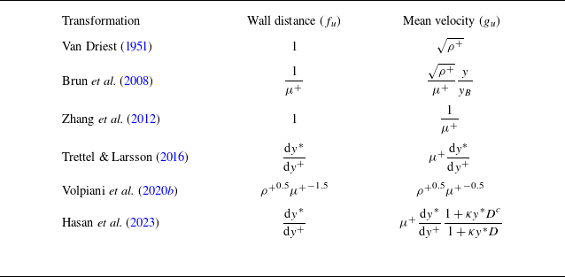
For compressible flows, however, (2.1) cannot be simplified to (2.2) owing to the enhanced compressibility and heat transfer. To map compressible flows onto their incompressible counterparts, velocity transformations are introduced as (Volpiani et al. Reference Volpiani, Iyer, Pirozzoli and Larsson2020b )
 \begin{align} {\textrm{d}}Y^+ = f_u {\textrm{d}}y^+,\qquad {\textrm{d}}U^+ = g_u {\textrm{d}}u^+, \end{align}
where
 $f_u$
and
 $g_u$
are the mapping functions for the wall distance and mean velocity, respectively, and the subscript
 $u$
represents the velocity. According to (2.3), the mean shear
 ${\textrm{d}}U^+/{\textrm{d}}Y^+$
can be expressed as
 \begin{align} \dfrac {{\textrm{d}}U^+}{{\textrm{d}}Y^+} = \dfrac {g_u}{f_u}\dfrac {{\textrm{d}}u^+}{{\textrm{d}}y^+}. \end{align}
Various velocity transformations (Van Driest Reference Van Driest1951; Brun et al. Reference Brun, Boiarciuc, Haberkorn and Comte2008; Zhang et al. Reference Zhang, Bi, Hussain, Li and She2012; Trettel & Larsson Reference Trettel and Larsson2016; Volpiani et al. Reference Volpiani, Iyer, Pirozzoli and Larsson2020b
; Hasan et al. Reference Hasan, Larsson, Pirozzoli and Pecnik2023) have been developed as detailed in Appendix B. Nevertheless, (2.4) is ill-suited to the multi-layered turbulence structure. To address this, Griffin et al. (Reference Griffin, Fu and Moin2021) proposed a hybrid transformation (the Griffin–Fu–Moin (GFM) transformation) to treat compressibility across different layers. Under the constant-stress-layer assumption (
 $\tau ^+ \approx 1$
), the total stress is expressed as
 \begin{align} \tau ^+ = \tau _\nu ^+ + \tau _R^+ =\dfrac {{\textrm{d}}U^+}{{\textrm{d}}Y^+}\left ( \dfrac {\tau _\nu ^+}{\mu ^+\dfrac {{\textrm{d}}u^+}{{\textrm{d}}y^+}} + \dfrac {\tau _R^+}{\dfrac {1}{\mu ^+}\dfrac {{\textrm{d}}u^+}{{\textrm{d}}y^*}} \right ), \end{align}
where
 $\tau _\nu ^+$
(
 $\tau _R^+$
) denotes the viscous (Reynolds) shear stress and
 $y^*=y^+\sqrt {\rho ^+}/\mu ^+$
represents the semi-local coordinate. From (2.5),
 ${\textrm{d}}U^+/{\textrm{d}}Y^+$
can achieve different approximations:
 ${\textrm{d}}U^+/{\textrm{d}}Y^+ \approx \mu ^+{\textrm{d}}u^+/{\textrm{d}}y^+$
when
 $\tau _\nu ^+ \gg \tau _R^+$
(viscous sublayer) and
 ${\textrm{d}}U^+/{\textrm{d}}Y^+ \approx (1/\mu ^+ ){\textrm{d}}u^+/{\textrm{d}}y^*$
when
 $\tau _\nu ^+ \ll \tau _R^+$
(logarithmic layer). The GFM transformation, derived from (2.5) (see Appendix B), has been validated across various compressible flows with adiabatic and isothermal walls (Griffin et al. Reference Griffin, Fu and Moin2021; Zhang et al. Reference Zhang, Wan, Liu, Sun and Lu2022; Cogo et al. Reference Cogo, Baù, Chinappi, Bernardini and Picano2023).
However, as the friction Mach number
 $M_\tau = u_\tau / (\gamma R T_w )^{1/2}$
rises, the IC effects increasingly impair the efficacy of
 ${\textrm{d}}U^+/{\textrm{d}}Y^+$
in compressible flows. The enhanced wall-normal pseudo-sound dilatational velocity suppresses quasi-streamwise vortices, thereby elevating
 $\tau _{\nu }^+$
in the buffer layer (Hasan et al. Reference Hasan, Costa, Larsson, Pirozzoli and Pecnik2025). According to (2.5), the increase in
 $\tau _{\nu }^+$
drives
 ${\textrm{d}}U^+/{\textrm{d}}Y^+$
toward
 $\mu ^+{\textrm{d}}u^+/{\textrm{d}}y^+$
, inducing an upward shift relative to the incompressible profile under
 $Y^+ = y^*$
(Hasan et al. Reference Hasan, Larsson, Pirozzoli and Pecnik2023).
Besides, the term
 $ (1/\mu ^+ ){\textrm{d}}u^+/{\textrm{d}}y^*$
in (2.5), which is generalised from the approximate balance of turbulence production and dissipation in the logarithmic region, proves insufficiently robust (Lee et al. Reference Lee, Helm, Martín and Williams2023; Younes & Hickey Reference Younes and Hickey2023). Notably, Cogo et al. (Reference Cogo, Salvadore, Picano and Bernardini2022) found that dissipation, along with the sum of turbulent production and transport, remains Mach independent for
 $y^+\gt 20$
. Therefore, (2.5) warrants refinement in the buffer and logarithmic layers (Younes & Hickey Reference Younes and Hickey2023).
To enhance the universality of
 $\tau _{\nu }^+$
in the buffer layer, the total stress balance between compressible flows and their incompressible counterparts is considered as follows (Hasan et al. Reference Hasan, Larsson, Pirozzoli and Pecnik2023):
 \begin{align} \left (\dfrac {\overline {\mu }}{\mu _w}+\dfrac {\mu _t^{com}}{\mu _w}\right )\dfrac {{\textrm{d}}u^+}{{\textrm{d}}y^+} \approx \left ( 1 +\dfrac {\mu _t^{in}}{\mu _w}\right )\dfrac {{\textrm{d}}U^+}{{\textrm{d}}Y^+}. \end{align}
Here
 $\mu _t^{com}$
can be prescribed via
 $\sqrt {\overline {\tau }_w\, \overline {\rho }} \kappa y D^c$
with
 $D^c = (1 - \exp (-y^*/ (A^+ + 19.3M_{\tau } ) ) )^2$
. From (2.6),
 ${\textrm{d}}U^+/{\textrm{d}}Y^+ \approx \phi _{\textit{ic}} \mu ^+{\textrm{d}}u^+/{\textrm{d}}y^+ = \tau _{c}^+$
follows, where
 $\phi _{\textit{ic}}= (1+\kappa y^*D^c )/ (1+\kappa y^*D )$
serves as the IC correction term. The modified shear stress
 $\tau _{c}^+$
exhibits superior universality across Mach numbers relative to
 $\tau _{\nu }^+$
(Hasan et al. Reference Hasan, Larsson, Pirozzoli and Pecnik2023). Accordingly, (2.5) is revised to
 \begin{align} 1=\dfrac {{\textrm{d}}U^+}{{\textrm{d}}Y^+}\left (\dfrac {\tau _{c}^+}{\dfrac {g_u^2}{f_u^2}\dfrac {{\textrm{d}}u^+}{{\textrm{d}}y^+}} + \dfrac { 1 - \tau _{c}^+ }{\dfrac {g_u^1}{f_u^1}\dfrac {{\textrm{d}}u^+}{{\textrm{d}}y^+}}\right )\!. \end{align}
Here,
 $g_u^1$
(
 $g_u^2$
) and
 $f_u^1$
(
 $f_u^2$
) are mapping functions for the mean velocity and wall-normal coordinate based on (2.3), respectively. Superscripts 1 and 2 denote distinct layers:
 $g_u^1$
and
 $f_u^1$
are adopted in the logarithmic layer (
 $\tau _c^+ \rightarrow 0$
), while
 $g_u^2$
and
 $f_u^2$
are employed below the buffer layer (
 $\tau _c^+ \rightarrow 1$
). Considering the efficacy of
 $\tau _{c}^+$
in the sub- and buffer layers, assuming that
 $ (g_u^2/f_u^2 ){\textrm{d}}u^+/{\textrm{d}}y^+ = \tau _{c}^+$
in (2.7), the proposed hybrid velocity transformation can be derived as
 \begin{align} \dfrac {{\textrm{d}}U^+}{{\textrm{d}}Y^+} = \dfrac {\dfrac {g_u^1}{f_u^1}\dfrac {{\textrm{d}}u^+}{{\textrm{d}}y^+}}{1- \phi _{\textit{ic}} \mu ^+ \dfrac {{\textrm{d}}u^+}{{\textrm{d}}y^+} + \dfrac {g_u^1}{f_u^1}\dfrac {{\textrm{d}}u^+}{{\textrm{d}}y^+}}. \end{align}
In contrast to the GFM transformation, (2.8) accounts for the IC effects through
 $\phi _{\textit{ic}}$
. To ensure consistency with the employed Mach-independent scaling below the buffer layer, the proposed hybrid transformation is integrated using the semi-local coordinate (
 $Y^+=y^*$
), which has proven effective for collapsing compressible profiles (Trettel & Larsson Reference Trettel and Larsson2016; Cogo et al. Reference Cogo, Baù, Chinappi, Bernardini and Picano2023; Cheng & Fu Reference Cheng and Fu2024b
). In the logarithmic layer,
 ${\textrm{d}}U^+/{\textrm{d}}Y^+$
approximates
 $ (g_u^1/f_u^1 ){\textrm{d}}u^+/{\textrm{d}}y^+$
according to (2.7). By fixing
 $f_u^1 = {\textrm{d}}y^*/{\textrm{d}}y^+$
,
 $g_u^1$
can be mined with the SR method detailed in § 3.
2.2. The temperature transformation
The temperature transformation can be derived from the mean energy balance, which is recast and non-dimensionalised as (see Appendix A)
 \begin{align} \left (\dfrac {\overline {\mu }/\mu _w}{\textit{Pr}}+\dfrac {\mu _t^{com}/\mu _w}{\textit{Pr}_t}\right )\dfrac {{\textrm{d}}\theta ^+}{{\textrm{d}}y^+}=B_q+\left (\gamma -1\right )M_{\tau }^2u^+, \end{align}
where
 $\theta ^+ = (T_w - \overline {T} )/T_w$
is the dimensionless temperature,
 $B_q=\overline {q}_w/ (\rho _w u_{\tau } c_p T_w )$
denotes the dimensionless wall heat flux and
 $\gamma$
is the specific heat ratio. The term
 $ (\gamma -1 )M_{\tau }^2u^+$
represents non-negligible viscous heating in compressible flows (Chen et al. Reference Chen, Huang, Shi, Yang and Lv2022a
). To preserve the structural similarity with the velocity equation (2.1), (2.9) can be rewritten as
 \begin{align} \left (\dfrac {\overline {\mu }/\mu _w}{\textit{Pr}}+\dfrac {\mu _t^{com}/\mu _w}{\textit{Pr}_t}\right )\dfrac {{\textrm{d}}\theta _s^+}{{\textrm{d}}y^+}=1, \end{align}
where
 $\theta _s^+$
is obtained by integrating
 ${\textrm{d}}\theta _s^+= {\textrm{d}}\theta ^+/ (B_q+ (\gamma -1 )M_{\tau }^2u^+ )$
with a zero wall value. For low-speed flows with
 $\overline {\mu } \approx \mu _w$
, (2.10) can be simplified to
 \begin{align} \dfrac {{\textrm{d}}\varTheta ^+}{{\textrm{d}}Y^+}=\dfrac {1}{\dfrac {1}{\textit{Pr}}+\dfrac {\mu _{\textit{t,in}}^+}{\textit{Pr}_t}}, \end{align}
with
 $\varTheta$
denoting the incompressible temperature. In (2.11),
 $\mu _{\textit{t,in}}^+$
is prescribed using the JK model (Johnson & King Reference Johnson and King1985), while
 $\textit{Pr}_t$
is parameterised as (Huang et al. Reference Huang, Coleman, Spalart and Yang2023)
 $\textit{Pr}_t = 1.05-0.2{\textrm{tanh}}^3 (Y^+/A_{\textit{Pr}}^+ )$
, where
 $A_{\textit{Pr}}^+ = 70$
. Consequently, the mean temperature profile for low-speed flows in the logarithmic layer (1.2) can be recovered.
As the Mach number increases, (2.10) cannot be simplified to (2.11) because of the significant viscous heating, and the diabatic wall boundary condition leads to the non-monotonic mean temperature profiles, thereby rendering the compressible mean temperature scaling more intricate. To address this, temperature transformations, which map compressible mean temperature profiles to the incompressible reference, have been explored. Analogous to
 $f_u$
and
 $g_u$
in (2.3), the temperature mapping functions are given by
 \begin{align} {\textrm{d}}Y^+ = f_T{\textrm{d}}y^+,\qquad {\textrm{d}}\varTheta ^+ = g_T{\textrm{d}}\theta _s^+, \end{align}
where the subscript
 $T$
represents the temperature. According to (2.12), the mean temperature gradient
 ${\textrm{d}}\varTheta ^+/{\textrm{d}}Y^+$
can be expressed as
 \begin{align} \dfrac {{\textrm{d}}\varTheta ^+}{{\textrm{d}}Y^+} = \dfrac {g_T}{f_T}\dfrac {{\textrm{d}}\theta _s^+}{{\textrm{d}}y^+}. \end{align}
Existing temperature transformations (Patel et al. Reference Patel, Boersma and Pecnik2017; Chen et al. Reference Chen, Huang, Shi, Yang and Lv2022a ; Huang et al. Reference Huang, Coleman, Spalart and Yang2023; Cheng & Fu Reference Cheng and Fu2024b ) can be expressed in the form of (2.13), as detailed in Appendix B. However, these temperature transformations demonstrate lower accuracy relative to the velocity counterparts (Chen, Gan & Fu Reference Chen, Gan and Fu2025). Analogous to the velocity fields, the multi-layered structure of turbulence should also be considered for the mean temperature profiles, thereby motivating the adoption of a hybrid form for the temperature transformation.
To bridge the Mach-invariant scalings across the different layers, the hybrid velocity transformation (2.8) is developed based on the modified shear stress
 $\tau ^+_c$
following Griffin et al. (Reference Griffin, Fu and Moin2021). For the mean temperature, similarly, a recently proposed Mach-invariant function
 $\phi _{\textit{ST}}$
is employed (Cheng & Fu Reference Cheng and Fu2024b
), and the following equation is formulated:
 \begin{align} 1 = \dfrac { {\textrm{d}}\varTheta ^+ }{ {\textrm{d}}Y^+ } \left ( \dfrac {\phi _{\textit{ST}}/\textit{Pr}}{ \dfrac {g_{T}^2}{f_{T}^2} \dfrac {{\textrm{d}}\theta _s^+}{{\textrm{d}}y^+} } + \dfrac { 1 - \phi _{\textit{ST}}/\textit{Pr} }{ \dfrac {g_{T}^1}{f_{T}^1} \dfrac {{\textrm{d}}\theta _s^+}{{\textrm{d}}y^+}} \right )\!. \end{align}
Here
 $g_T^1$
(
 $g_T^2$
) and
 $f_T^1$
(
 $f_T^2$
) are mapping functions for the mean temperature and wall-normal coordinate based on (2.12):
 $g_T^1$
and
 $f_T^1$
are adopted in the logarithmic layer, while
 $g_T^2$
and
 $f_T^2$
are employed in the viscous sublayer. The Mach-invariant function
 $\phi _{\textit{ST}}=\sqrt {\rho ^+}{\textrm{d}}\theta _s^+/{\textrm{d}}y^*$
can also transfer the compressible temperature gradient to the ‘incompressible’ state in principle (Cheng & Fu Reference Cheng and Fu2024b
). The ‘incompressible’ temperature gradient
 ${\textrm{d}}\varTheta ^+/{\textrm{d}}Y^+$
(2.11) approaches
 $\textit{Pr}$
in the viscous sublayer (where
 $\mu _{\textit{t,in}}^+ \rightarrow 0$
) and approaches 0 in the logarithmic region (where
 $\mu _{\textit{t,in}}^+ \propto y^+$
). Consequently,
 $\phi _{\textit{ST}}$
/
 $ \textit{Pr} \rightarrow 1$
in the viscous sublayer and
 $\phi _{\textit{ST}}$
/
 $ \textit{Pr} \rightarrow 0$
in the logarithmic region. In (2.14),
 $\phi _{\textit{ST}}/ \textit{Pr}$
performs analogously to
 $\tau _{c}^+$
in (2.7). Furthermore, (2.14) coupled with other Mach-invariant functions (Patel et al. Reference Patel, Boersma and Pecnik2017; Hasan et al. Reference Hasan, Larsson, Pirozzoli and Pecnik2023; Zhu et al. Reference Zhu, Zhang, Yang, Ji and Xia2025a
), such as
 $\phi _{{\textit{TL}}\mbox{-}{T}}=\mu ^+{\textrm{d}}\theta _s^+/{\textrm{d}}y^+$
and
 $\phi _{\textit{HLPP}}$
=
 $\phi _{\textit{ic}}\phi _{{\textit{TL}}\mbox{-}{\textit{T}}}$
, is discussed in Appendix C.
In (2.14) the mapping functions (
 $f_{T}^1$
,
 $f_{T}^2$
,
 $g_{T}^1$
and
 $g_{T}^2$
) must be determined. For simplification, assuming that
 $ (g_{T}^2/f_{T}^2 ){\textrm{d}}\theta _s^+/{\textrm{d}}y^+ = \sqrt {\rho ^+} {\textrm{d}}\theta _s^+/{\textrm{d}}y^*$
, the proposed hybrid temperature transformation is
 \begin{align} \dfrac {{\textrm{d}}\varTheta ^+}{{\textrm{d}}Y^+} = \dfrac { \textit{Pr}* \dfrac {g_{T}^1}{f_{T}^1} \dfrac {{\textrm{d}}\theta _s^+}{{\textrm{d}}y^+}}{ \textit{Pr} -\sqrt {\rho ^+} \dfrac {{\textrm{d}}\theta _s^+}{{\textrm{d}}y^*} + \dfrac {g_{T}^1}{f_{T}^1} \dfrac {{\textrm{d}}\theta _s^+}{{\textrm{d}}y^+}}. \end{align}
Equation (2.15) can be integrated using the semi-local coordinate (
 $Y^+=y^*$
), which is consistent with the work of Cheng & Fu (Reference Cheng and Fu2024b
). Similar to the hybrid velocity transformation (2.8), in the logarithmic layer (where
 $\phi _{\textit{ST}}/\textit{Pr}$
approaches 0),
 $f_{T}^1={\textrm{d}}y^*/{\textrm{d}}y^+$
is fixed and
 $g_{T}^1$
can be discovered with the SR method outlined in § 3.
Finally, the efficacy of the aforementioned transformations can be evaluated using the following metrics. The integrated percent errors (
 $\epsilon$
) for mean velocity and temperature profiles are defined as (Griffin et al. Reference Griffin, Fu and Moin2021)
 \begin{align} \epsilon _{u} = \dfrac {\int _{0}^{0.3Re_{T}}\left |U_a^+-U^+\right |{\textrm{d}}Y^+}{\int _{0}^{0.3Re_{T}}U^+{\textrm{d}}Y^+}, \quad \epsilon _{T} = \dfrac {\int _{0}^{y^+ \mid _{Y^+=0.3Re_{T}}}\left |T_m^+-T^+\right |{\textrm{d}}y^+}{\int _{0}^{y^+ \mid _{Y^+=0.3Re_{T}}}T^+{\textrm{d}}y^+}, \end{align}
where
 $Re_{T}=Y^+\mid _{y=\delta _{99}}$
and
 $\delta _{99}$
is determined at
 $\widetilde {u}=0.99\widetilde {u}_e$
(subscript
 $e$
denoting free-stream quantities). Here
 $U_a^+$
represents the transformed mean velocity,
 $T^+=\overline {T}/T_w$
and
 $T_m^+$
denotes the predicted mean temperature. We adopt an upper integration bound at 0.3
 $Re_{T}$
, which encompasses both sub- to logarithmic layers across varying Mach numbers and wall thermal conditions (Griffin, Fu & Moin Reference Griffin, Fu and Moin2023). To avoid discontinuities in
 $\theta _s^+$
arising from
 $B_q+(\gamma -1)M_{\tau }^2u^+=0$
,
 $T_m^+$
is adopted for evaluating the temperature transformations. Based on (2.13),
 $T_m^+$
can be derived from
 $\varTheta ^+$
(2.11) as follows:
 \begin{align} \dfrac {{\textrm{d}}T_m^+}{{\textrm{d}}y^+} = -\left (B_q+(\gamma -1)M_{\tau }^2u^+\right ) \dfrac {f_T}{g_T} \dfrac {{\textrm{d}}\varTheta ^+}{{\textrm{d}}Y^+}. \end{align}
For the hybrid temperature transformations, the inversion equation is
 \begin{align} \dfrac {{\textrm{d}}T_m^+}{{\textrm{d}}y^+} = \left (\dfrac {-(B_q+(\gamma -1)M_{\tau }^2u^+)}{ \dfrac {g_{T}^1}{f_{T}^1}\left (1-\dfrac {1}{\textit{Pr}}\dfrac {{\textrm{d}}\varTheta ^+}{{\textrm{d}}Y^+} \right ) + \sqrt {\rho ^+}\dfrac {{\textrm{d}}y^+}{{\textrm{d}}y^*}\dfrac {1}{\textit{Pr}} \dfrac {{\textrm{d}}\varTheta ^+}{{\textrm{d}}Y^+}}\right ) \dfrac {{\textrm{d}}\varTheta ^+}{{\textrm{d}}Y^+}. \end{align}
Overall, this section derives the proposed hybrid velocity and temperature transformations ((2.8) and (2.15)). However, the mapping functions
 $g_u^1$
and
 $g_T^1$
remain undetermined. In § 3 we introduce the PISR method to discover these specific mapping functions.
3. Methods
3.1. Dataset
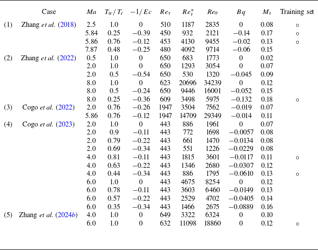
To establish and evaluate the velocity and temperature transformations, 25 published DNS cases of compressible TBLs are employed, with free-stream Mach numbers in the range 0.5–8 and the friction Reynolds numbers in the range 443–1947, as listed in table 1 (Zhang et al. Reference Zhang, Duan and Choudhari2018, Reference Zhang, Wan, Liu, Sun and Lu2022; Cogo et al. Reference Cogo, Salvadore, Picano and Bernardini2022, Reference Cogo, Baù, Chinappi, Bernardini and Picano2023; Zhang et al. Reference Zhang, Wan, Sun and Lu2024b
). Figure 2 presents the phase diagrams of the Mach number versus the wall-to-recovery-temperature ratio and the negative reciprocal of the Eckert number (
 $-1/Ec$
), where
 $Ec$
is defined as (Gibis et al. Reference Gibis, Sciacovelli, Kloker and Wenzel2024)
 \begin{align} Ec = \dfrac { (\gamma -1) Ma^2T_e}{T_r - T_w}. \end{align}
Here,
 $T_r=T_e(1+r(\gamma -1)/2Ma^2)$
denotes the recovery temperature, with recovery factor
 $r = 0.89$
. As illustrated in figure 2(b),
 $-1/Ec$
varies from –0.54 to 0, covering adiabatic, weak cooling, moderate cooling and strong cooling conditions (Gibis et al. Reference Gibis, Sciacovelli, Kloker and Wenzel2024). To discover the undetermined mapping functions using the dataset, the PISR method is introduced and elaborated in the following subsection.
Summary of parameters from the compressible TBL dataset used in this study. The friction Reynolds number is defined as
 $Re_{\tau } = \rho _w u_{\tau }\delta _{99}/\mu _w$
, the semi-local friction Reynolds number as
 $Re_{\tau }^* = \sqrt {\rho _e \overline {\tau }_w} \delta _{99}/\mu _e$
and the Reynolds number based on momentum thickness as
 $Re_{\theta } = \rho _e u_e \theta / \mu _e$
. Circles (
 $\circ$
) represent the training set.

Collection of compressible DNS at different Mach numbers plotted over (a) the wall-to-recovery-temperature ratio
 $T_w/T_r$
, and (b) the negative reciprocal of the Eckert number
 $-1/Ec$
. Dashed lines in (b) distinguish regions of different heat-transfer effects.

3.2. Physics-informed SR method
In SR, purely data-driven approaches typically require extensive datasets to reliably identify underlying functional relations, owing to the inherently large optimisation search space. However, this poses significant challenges in experimental or computational set-ups characterised by high costs or scarce data, such as compressible TBLs investigated in this work. To mitigate these constraints, the proposed hybrid transformations ((2.8) and (2.15)) confine the scaling of undetermined mapping functions
 $g_u$
(
 $g_T$
) to the logarithmic layer, rather than the entire inner layer. Accordingly, by embedding this prior physical knowledge into the SR framework, a novel approach named PISR is proposed. The PISR method effectively constrains the optimisation search space, transforming a traditionally broad data-driven problem into a more targeted and physically coherent equation closure challenge. Algorithmically, the PISR integrates symbolic mathematics with reinforcement learning methods, which are effective in discovering implicit governing equations (Du et al. Reference Du, Chen and Zhang2024) and mapping functions.
3.2.1. Generating the optimal mapping functions with PISR
In PISR a potential mapping function can be represented as a unique symbolic traversal with a binary tree serving as the bridge between the function and the symbolic traversal. The following discussion addresses two key aspects: (i) conversion from the symbolic traversal to a binary tree, (ii) transformation of the binary tree into a function. As illustrated in figure 3(a), each symbol in the traversal corresponds to a distinct node in the binary tree. The symbols are categorised as operators (
 $\times ,\, \div , \, +, \, \sqrt {\hphantom {x}}$
) or operands (
 $a_1,\, a_2,\, a_3,\, a_4$
), with interior nodes corresponding to operators and leaf nodes to operands. The red arrows in figure 3(a) delineate the conversion path: starting from the root node (
 $\sqrt {\hphantom {x}}$
), it processes the left child node first until reaching the leaf node (e.g.
 $\sqrt {\hphantom {x}},\,\div , \,+ ,\, a_1$
), then returns to the nearest operator node whose child nodes are not full and enters the other branch (e.g.
 $a_2$
). The conversion ceases once all operator nodes attain full child nodes. Subsequently, the binary tree can be transformed into a function. The operator nodes with their child nodes can be seen as calculation units (highlighted by blue and yellow boxes in figure 3
a). Therefore, the depicted tree represents the division of
 $a_1 + a_2$
by
 $a_3 \times a_4$
followed by a square root.
(a) Schematic diagram of a binary tree, which bridges the function and symbolic traversal in the PISR framework. (b) Flow chart to mine the undetermined mapping functions
 $g_u^1$
and
 $g_T^1$
in hybrid transformations (2.8) and (2.15) through the PISR method (purple box). The generation process (green arrow) in the PISR is detailed in the green dashed box.

Figure 3(b) illustrates the workflow of the PISR. Initially, a comprehensive symbol library must be predefined. For the velocity transformation, the key symbols employed are
 \begin{align} \rho ^+, \,T^+, \,\mu ^+, \,y^+, \,y^*, \,\dfrac {{\textrm{d}}y^*}{{\textrm{d}}y^+}, \,\dfrac {{\textrm{d}}T^+}{{\textrm{d}}y^+}, \,\dfrac {{\textrm{d}}T^+}{{\textrm{d}}y^*}, \,\times , \,\div , \, \sqrt {\hphantom {x}} , \, \partial , \,+. \end{align}
Here,
 $\rho ^+$
and
 $T^+$
directly reflect the compressibility effects;
 $\mu ^+$
is a function of temperature with Sutherland’s law;
 $y^+,\,y^*$
and
 ${\rm d}y^*/{\rm d}y^+$
are associated with the semi-local coordinates. Additionally, the mean temperature gradients (
 ${\textrm{d}}T^+/{\textrm{d}}y^+$
and
 ${\textrm{d}}T^+/{\textrm{d}}y^*$
) are derived from the mean enthalpy gradient, which was adopted as a dimensionless parameter for compressible TBLs by Vigdorovich (Reference Vigdorovich2023). Meanwhile, operators (
 $\times , \div$
,
 $\sqrt {\hphantom {x}}$
and
 $\partial$
) are drawn from established transformations (as detailed in Appendix B) and
 $+$
is also introduced for more choices. For mining the temperature transformation, the temperature
 $T^+$
in (3.2) is substituted by the velocity
 $u^+$
.
Then, the PISR reads the symbol library and identifies the optimal mapping function, which is composed of predefined symbols. As indicated by the green arrow in figure 3(b), a long–short-term memory (LSTM) agent generates candidate functions for
 $g_u^1$
(
 $g_T^1$
) by sampling from the symbol library. The green dashed box in figure 3(b) exemplifies this generation process. The LSTM agent incorporates both global and local inputs to produce a probability distribution over the symbols, incorporating constraints on traversal length, symbol occurrence frequencies and other relevant factors (Du et al. Reference Du, Chen and Zhang2024). The final distribution is normalised, from which the symbol with the maximum probability is selected.
Following the generation process, the 500 candidate mapping functions are substituted into the proposed hybrid transformation to compute the transformed mean velocity
 $U_a^+$
(and predicted mean temperature
 $T_m^+$
) with the training set outlined in table 1. The training set consists of seven cases selected to cover the parameter space of the full dataset. The mean integrated percent errors in the established profiles (2.16) across the training set are imported into the reward functions as
 \begin{align} r_u = \dfrac {1}{1+\overline {\epsilon }_u}, \quad r_T = \dfrac {1}{1+\overline {\epsilon }_T}. \end{align}
To maintain balance between the viscous sub- and logarithmic layers during the training process, a narrower upper limit
 $y=0.3\delta _{99}$
is employed in (3.3) for
 $\overline {\epsilon }_u$
and
 $\overline {\epsilon }_T$
. These rewards
 $r_u$
and
 $r_T$
quantify the efficacy of the candidate mapping functions. At the first training epoch, the highest-reward candidate is recorded as the best mapping function. In subsequent training epochs, this incumbent is compared against the top candidate from the new collection, with iterative updates to retain the superior performer. After
 $100$
training epochs, the optimal mapping function is generated, along with nine suboptimal alternatives for further selection.
To iteratively optimise the LSTM agent, the rewards of the candidate functions are employed in the optimisation process with the risk-seeking policy gradient approach (Du et al. Reference Du, Chen and Zhang2024). Specifically, the
 $\varepsilon =0.02$
quantile of the candidate functions is selected for training based on their rewards. The optimisation objective of the risk-seeking policy is formulated as
 \begin{align} J_{\textit{risk}}(\theta ;\varepsilon ) \doteq \mathbb{E}_{\tau \sim p(\tau \mid \theta )} [ r(\tau ) \mid r(\tau ) \geqslant \widetilde {q}_{\varepsilon }(r) ], \end{align}
where
 $\theta$
refers to the parameters of the LSTM agent,
 $\tau$
represents a candidate mapping function and
 $r(\tau )$
is its corresponding rewards;
 $p(\tau \mid \theta )$
denotes the probability distribution of generating
 $\tau$
under the current
 $\theta$
and
 $\widetilde {q}_{\varepsilon }(r)$
represents the threshold for selecting candidate mapping functions for training. The gradient of (3.4) can be approximated as (see Appendix D)
 \begin{align} \boldsymbol{\nabla} _{\theta }J_{ {risk}}(\theta ;\varepsilon ) \approx \dfrac {\lambda _{pg}}{\varepsilon N} \sum _{i=1}^{N} [ r(\tau ^{(i)}) - \widetilde {q}_{\varepsilon }(r) ] \boldsymbol{\cdot }\boldsymbol{\nabla} _{\theta } {\textrm{log}} \,p(\tau ^{(i)} \mid \theta ), \end{align}
with
 $N$
denoting the total number of selected candidate mapping functions and
 $\lambda _{pg}$
measuring the importance of rewards. Additionally, the maximum entropy reinforcement learning (see Appendix D) is also combined to prevent generating a certain action continuously (Haarnoja et al. Reference Haarnoja, Zhou, Abbeel and Levine2018; Du et al. Reference Du, Chen and Zhang2024). Therefore, iterative optimisation of the agent enables improvement of the best result.
3.2.2. Transformations discovered by PISR
Building upon (2.8) and (2.15), the undetermined mapping functions
 $g_u^1$
and
 $g_{T}^1$
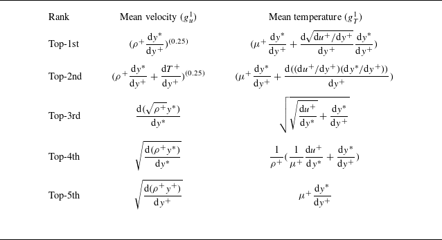
are discovered using the PISR method. Employing the training set in table 1, PISR yields
 $g_u^1 = (\rho ^+ {\textrm{d}}y^*/{\textrm{d}}y^+ )^{ (0.25 )}$
and
 $g_{T}^1 = \mu ^+ {\textrm{d}}y^*/{\textrm{d}}y^+ + ( {\textrm{d}} \sqrt {{\textrm{d}}u^+/{\textrm{d}}y^+} / {\textrm{d}}y^+ ) {\textrm{d}}y^*/{\textrm{d}}y^+$
. Accordingly, the proposed hybrid velocity and temperature transformations (HT-u and HT-T) are, respectively,
 \begin{align} \dfrac {{\textrm{d}}U^+}{{\textrm{d}}Y^+} &= \dfrac {\left (\rho ^+ \dfrac {{\textrm{d}}y^*}{{\textrm{d}}y^+} \right )^{\left (0.25\right )}\dfrac {{\textrm{d}}u^+}{{\textrm{d}}y^*}}{1- \phi _{\textit{ic}} \mu ^+ \dfrac {{\textrm{d}}u^+}{{\textrm{d}}y^+}+ \left (\rho ^+ \dfrac {{\textrm{d}}y^*}{{\textrm{d}}y^+} \right )^{(0.25)}\dfrac {{\textrm{d}}u^+}{{\textrm{d}}y^*}}, \\[-12pt] \nonumber \end{align}
 \begin{align} \dfrac {{\textrm{d}}\varTheta ^+}{{\textrm{d}}Y^+} &= \dfrac {\textit{Pr} \left ( \mu ^+ \dfrac {{\textrm{d}}y^*}{{\textrm{d}}y^+} + \dfrac {{\textrm{d}} \sqrt {{\textrm{d}}u^+/{\textrm{d}}y^+}}{{\textrm{d}}y^+} \dfrac {{\textrm{d}}y^*}{{\textrm{d}}y^+} \right ) \dfrac {{\textrm{d}}\theta _s^+}{{\textrm{d}}y^*}}{ \textit{Pr} -\sqrt {\rho ^+} \dfrac {{\textrm{d}}\theta _s^+}{{\textrm{d}}y^*} + \left ( \mu ^+ \dfrac {{\textrm{d}}y^*}{{\textrm{d}}y^+} + \dfrac {{\textrm{d}} \sqrt {{\textrm{d}}u^+/{\textrm{d}}y^+}}{{\textrm{d}}y^+} \dfrac {{\textrm{d}}y^*}{{\textrm{d}}y^+} \right ) \dfrac {{\textrm{d}}\theta _s^+}{{\textrm{d}}y^*}}. \end{align}
Overall, the PISR yields novel mapping functions that align closely with established physical insights. For the velocity field, we note that Younes & Hickey (Reference Younes and Hickey2023) proposed
 $\sqrt {\rho ^+}{\textrm{d}}u^+/{\textrm{d}}y^*$
(with
 $g_u=\sqrt {\rho ^+}$
and
 $f_u={\textrm{d}}y^*/{\textrm{d}}y^+$
) for the scaling in the logarithmic layer, which represents a semi-local normalised mean spanwise vorticity. Likewise, the GFM transformation’s
 $g_u=1/\mu ^+$
(from
 $(1/\mu ^+){\textrm{d}}u^+/{\textrm{d}}y^*$
) can be approximated to
 $(\rho ^+)^{0.7}$
(
 $\mu ^+ \approx (T^+)^{0.7} \approx (\rho ^+)^{-0.7}$
). The PISR form
 $ (\rho ^+{\textrm{d}}y^*/{\textrm{d}}y^+ )^{0.25}$
can be approximated to
 $(\rho ^+)^{0.55}$
with
 ${\textrm{d}}y^*/{\textrm{d}}y^+ \approx (\rho ^+)^{1.2}$
(neglecting the gradients of mean properties). Therefore,
 $ (\rho ^+{\textrm{d}}y^*/{\textrm{d}}y^+ )^{0.25}$
is similar to the scalings employed in the GFM transformation and proposed by Younes & Hickey (Reference Younes and Hickey2023). For the temperature field, the PISR-derived
 $g_{T}^{\textit{PISR}}=\mu ^+ {\textrm{d}}y^*/{\textrm{d}}y^+ + ( {\textrm{d}} \sqrt {{\textrm{d}}u^+/{\textrm{d}}y^+} / {\textrm{d}}y^+ ) {\textrm{d}}y^*/{\textrm{d}}y^+$
closely resembles the TL-type transformation
 $g_{T}^{\textit{TL}} = \mu ^+ {\textrm{d}}y^*/{\textrm{d}}y^+$
, augmented by an additional small term. Their performance is systematically evaluated in § 4. Besides, the suboptimal mapping functions obtained from the PISR are presented in Appendix E.
4. Results
In this section the proposed hybrid velocity and temperature transformations (HT-u and HT-T) are compared with GFM and the transformations proposed by Hasan et al. (Reference Huang, Coleman, Spalart and Yang2023) (denoted as HLPP), Huang et al. (Reference Huang, Coleman, Spalart and Yang2023) (denoted as TL-T) and Cheng & Fu (Reference Cheng and Fu2024b ) (denoted as ST) detailed in Appendix B. The transformed velocity profiles obtained from the HT-u model, alongside the predicted mean temperature profiles from the HT-T model are assessed. Moreover, the inverse HT-u and HT-T formulations are utilised to forecast compressible mean velocity and temperature profiles based solely on wall conditions.
4.1. The transformed velocity profiles
Existing studies have developed transformations to map the compressible mean velocity profiles to their incompressible counterparts. For instance, the transformed velocity profiles from the HLPP and GFM transformations are presented in figure 4(a). The HLPP-transformed velocity profiles (grey lines) deviate more substantially from the incompressible law of the wall (2.2) than those of the GFM transformation for
 $y^*\gt 30$
, underscoring the need for compressibility adjustments in the logarithmic layer. For the GFM transformation, the transformed velocity profiles exhibit upward shifts relative to the incompressible profile near
 $y^*=30$
, attributable to the limited universality of
 $\tau _\nu ^+$
across most cases in (2.5). Additionally, the mean profiles diverge downward from the incompressible reference in the logarithmic layer for the cases at
 $ \textit{Ma}=5.84,\, T_w/T_r=0.25$
and
 $ \textit{Ma}=8,\, T_w/T_r=0.25$
. In contrast, figure 4(b) illustrates that the transformed mean velocity profiles predicted by the HT-u transformation collapse robustly to the incompressible reference. In the buffer layer, the
 $\tau _c^+$
term employed in (2.7) demonstrates greater universality than
 $\tau _\nu ^+$
(Hasan et al. Reference Hasan, Larsson, Pirozzoli and Pecnik2023). For example, the root-mean-square error relative to the incompressible reference (
 $U_{a,rms}^+/U^+$
) is 2.93 % for GFM and 1.82 % for HT-u at
 $y^*=30$
across the dataset, respectively. Furthermore, the downward deviations in the GFM model for the aforementioned high-Mach, cold wall cases (
 $ \textit{Ma}=5.84, T_w/T_r=0.25$
and
 $ \textit{Ma}=8,\, T_w/T_r=0.25$
) are improved by the HT-u transformation, highlighting the efficacy of the PISR-mined
 $g_u^1$
in the logarithmic layer.
Comparison of transformed velocity profiles predicted by the (a) GFM and (b) HT-u transformations. The integrated percent error
 $\epsilon _u$
in the transformed velocity profiles are plotted versus (c) the Mach number and (d) the negative reciprocal of the Eckert number
 $-1/Ec$
, respectively.

Figure 4(c) presents the integrated percent error
 $\epsilon _u$
as a function of Mach number (
 $ \textit{Ma}$
). The data-driven velocity transformation from Volpiani et al. (Reference Volpiani, Iyer, Pirozzoli and Larsson2020b
) – referred to as the VIPL transformation – is also included. For
 $ \textit{Ma}\lt 3$
, most
 $\epsilon _u$
remains below 2 % across all models. However, with increasing
 $ \textit{Ma}$
, the HLPP transformation exhibits poor performance, consistent with the grey lines in figure 4(a,b). For instance,
 $\epsilon _u$
from the HLPP transformation reaches 9.04 % at
 $ \textit{Ma}=6, T_w/T_r=1$
, whereas those from the VIPL, GFM and HT-u transformations are 2.02 %, 2.19 % and 1.39 %, respectively. Figure 4(d) illustrates
 $\epsilon _u$
vs
 $-1/Ec$
. The performance of the HLPP transformations shows limited dependence on
 $Ec$
. However,
 $\epsilon _u$
for the GFM transformation rises as
 $-1/Ec$
decreases. At
 $ \textit{Ma} \geqslant 4$
,
 $M_{\tau }$
apparently increases with intensified wall cooling, leading to the upward shifts in the buffer layer. For example,
 $\epsilon _u$
from the GFM transformation increases from 0.87 % at
 $ \textit{Ma}=8,\, T_w/T_r=1$
(
 $-1/Ec=0$
) to 0.98 % at
 $ \textit{Ma}=8,\, T_w/T_r=0.5$
(
 $-1/Ec=-0.25$
) and 4.41 % at
 $ \textit{Ma}=8,\, T_w/T_r=0.25$
(
 $-1/Ec=-0.37$
), respectively. Ultimately, the HT-u transformation demonstrates superior accuracy relative to both the HLPP and GFM transformations, and does not significantly vary with
 $ \textit{Ma}$
and
 $Ec$
. The shortcomings of the GFM transformation are improved through the incorporation of the IC correction term
 $\phi _{\textit{ic}}$
and PISR-derived
 $g_u^1$
in (3.6). Across the dataset, the mean
 $\epsilon _u$
declines from 4.98 % (HLPP), 1.91 % (VIPL) and 1.67 % (GFM) to 0.96 % (HT-u). The ‘incompressible’ indicator functions (
 $Y^+{\textrm{d}}U^+/{\textrm{d}}Y^+$
) are also presented in figure 5. The profiles predicted by the HT-u transformation are consistent with the incompressible profile. For example, the root-mean-square errors of
 $Y^+{\textrm{d}}U^+/{\textrm{d}}Y^+$
relative to the incompressible reference at
 $Y^+=10$
are 3.42 % (HLPP), 7.4 % (VIPL), 5.19 % (GFM) and 2.74 % (HT-u), respectively.
Comparison of the ‘incompressible’ indicator functions (
 $Y^+{\textrm{d}}U^+/{\textrm{d}}Y^+$
), which are predicted by the (a) HLPP, (b) VIPL, (c) GFM and (d) HT-u transformations. The dashed lines denote the incompressible reference obtained from (2.2).

To further delineate the contributions of
 $\phi _{\textit{ic}}$
and
 $g_u^1$
in (2.8), the performance of transformations at
 $ \textit{Ma}=4,\, T_w/T_r=0.44$
is illustrated in figure 6(a). Relative to the GFM transformation, the HLPP-transformed velocity profile aligns more closely with the incompressible reference in the buffer layer, highlighting the importance of IC effects. The integrated percent error decreases from 3.57 % (GFM) to 1.10 % (HLPP) within
 $10\lt y^*\lt 50$
. To isolate the role of
 $\phi _{\textit{ic}}$
, a modified GFM transformation (M-GFM) is introduced by substituting
 $g_u^1 = 1/\mu ^+$
in (2.8). The M-GFM transformation achieves excellent agreement with the incompressible law of the wall for
 $y^*\lt 0.3Re_T$
, confirming that the incorporation of
 $\phi _{\textit{ic}}$
in (2.8) effectively eliminates the upward shifts seen in the GFM transformation. Nevertheless, as presented in figure 6(b), the M-GFM transformation deviates more from the incompressible reference than the GFM transformation at
 $ \textit{Ma}=5.84, T_w/T_r=0.25$
, indicating that the downshift behaviour at
 $y^*\gt 30$
(where
 $\tau _\nu ^+ \ll \tau _R^+$
) comes from
 $(1/\mu ^+){\textrm{d}}u^+/{\textrm{d}}y^*$
in (2.5). The HT-u transformation yields the greatest improvement over other models, owing to the PISR-derived
 $g_u^1$
in (2.8). The integrated percent error
 $\epsilon _u$
reduces from 4.64 % (HLPP) and 4.15 % (GFM) to 0.30 % (HT-u) in this case.
Comparison of transformed velocity profiles for (a)
 $ \textit{Ma}=4,T_w/T_r=0.44$
and (b)
 $ \textit{Ma}=5.84,T_w/T_r=0.25$
. The shaded region denotes the upper limit (
 $y^*=0.3Re_{T}$
).

4.2. The predicted mean temperature profiles
The mean temperature scaling can be derived through temperature transformations. To demonstrate the enhancements of the proposed HT-T transformation over the ST and TL-T transformations, the transformed temperature gradients are shown in figure 7. For
 $y^*\lt 5$
,
 $y^*\phi _{\textit{ST}}$
closely aligns with the ideal profile
 $y^*\phi _{ideal}$
(
 $Y^+{\textrm{d}}\varTheta ^+/{\textrm{d}}Y^+$
) derived from (2.11). However, it deviates downward from
 $y^*\phi _{ideal}$
for
 $y^*\gt 20$
. As illustrated in figure 7(b),
 $y^*\phi _{{\textit{TL}}\mbox{-}{T}}$
matches
 $y^*\phi _{ideal}$
well in the adiabatic cases (solid lines). For diabatic cases (dotted lines),
 $y^*\phi _{{\textit{TL}}\mbox{-}{T}}$
outperforms
 $y^*\phi _{\textit{ST}}$
at
 $y^*\gt 20$
but falls below
 $y^*\phi _{ideal}$
for
 $y^*\lt 5$
. Given the analogies between the velocity and temperature fields, it is unsurprising that the ST and TL-T transformations, which are generalised from the velocity transformations, exhibit regime-specific limitations. For instance, at
 $y^*=3$
,
 $y^*\phi _{\textit{ST}}$
achieves a lower root-mean-square error (
 $\epsilon _{ {rms}}$
) relative to
 $y^*\phi _{\textit{ideal}}$
of 7.78 %, versus 11.39 % for
 $y^*\phi _{{\textit{TL}}\mbox{-}{T}}$
. Conversely, at
 $y^*=50$
,
 $\epsilon _{ {rms}}$
values are 21.9 % for
 $y^*\phi _{\textit{ST}}$
and 11.67 % for
 $y^*\phi _{{\textit{TL}}\mbox{-}{T}}$
. As shown in figure 7(c),
 $\phi _{\textit{HT}\mbox{-}{T}}$
performs well for both regimes (
 $y^*\lt 5$
and
 $y^*\gt 20$
), achieving
 $\epsilon _{ {rms}}$
of 8.43 % at
 $y^*=3$
and 11.57 % at
 $y^*=50$
. According to (2.14),
 $\phi _{\textit{HT-T}} \approx \phi _{\textit{ST}}$
at
 $y^*\lt 5$
. Therefore, the HT-T transformation inherits the strengths of the ST transformation in the viscous sublayer. For
 $y^*\gt 20$
, the results show that the mapping function
 $g_{T}^1$
in (2.14) can be mined from the PISR method, collapsing both the adiabatic and cold wall data effectively.
The gradient of transformed temperature profiles multiplied by the semi-local coordinate (
 $y^*\phi$
) for the (a) ST, (b) TL-T and (c) HT-T transformations. The insets magnify the profiles in the viscous sublayer.

Due to the transformed temperature profiles exhibiting discontinuities at cold walls where
 $B_q+(\gamma -1)M_{\tau }^2u^+=0$
, the compressible mean temperature profiles predicted from the transformations are evaluated in figure 8(a). The ST transformation performs well in the viscous sublayer but falls below the DNS data as
 $y^+$
increases. For example, the relative error of mean temperature
 $e_T=|T^+ -T_{m}^+|/T^+$
from the ST transformation reaches 3.21 %, 19.59 % and 29.51 % at
 $y^+=10,50$
and 100 for
 $ \textit{Ma}=8,\,T_w/T_r=1$
, respectively. In contrast, the TL-T transformation outperforms in the logarithmic layer, with
 $e_T = 10.83\,\%$
at
 $y^+=100$
for the same case. However, as
 $-1/Ec$
decreases, the peaks of the profiles predicted by the TL-T model exceed the DNS profiles, with
 $e_T$
at the peak rising from 0.53 % (
 $ \textit{Ma}=4,\,T_w/T_r=0.63$
) to 2.42 % (
 $ \textit{Ma}=6,\,T_w/T_r=0.35$
) and 3.74 % (
 $ \textit{Ma}=8,\,T_w/T_r=0.25$
). For further comparison, a hybrid temperature transformation (HT-TL) is introduced using
 $g_T^1 = \mu ^+{\textrm{d}}y^*/{\textrm{d}}y^+$
in (2.15). Both the HT-TL and HT-T models achieve excellent performance in sub- and logarithmic layers while accurately capturing profile peaks. Compared with the ST model,
 $e_T$
at
 $y^+=100$
decreases from 29.51 % (ST) and 10.83 % (TL-T) to 1.33 % (HT-TL) and 1.17 % (HT-T) for
 $ \textit{Ma}=8,\,T_w/T_r=1$
. At the peaks of DNS profiles, the HT-TL transformation yields
 $e_T = 0.65\,\%$
for
 $ \textit{Ma}=6,\,T_w/T_r=0.35$
and 1.22 % for
 $ \textit{Ma}=8,\,T_w/T_r=0.25$
, while the HT-T transformation attains 0.66 % and 1.21 %, respectively. These results demonstrate the efficacy of layer-specific effective scalings for the mean temperature field.
(a) Comparison of mean temperature profiles predicted by the ST, TL-T, HT-TL and HT-T transformations against the DNS data. (b) The integrated percent error in mean temperature profiles
 $\epsilon _T$
, with the inset showing the mean integrated percent error
 $\overline {\epsilon }_T$
for each model across Mach number groups:
 $ \textit{Ma}$
= 2–2.5,
 $ \textit{Ma}=4$
,
 $ \textit{Ma} \approx 6$
and
 $ \textit{Ma} \approx 8$
.

Figure 8(b) presents the integrated percent error
 $\epsilon _T$
. The ST transformation demonstrates a poor performance, with
 $\overline {\epsilon }_T$
, defined as the mean
 $\epsilon _T$
across the dataset, of 11.02 %, and
 $\epsilon _T^m$
, which denotes the maximum error across the dataset, reaching 40.01 % at
 $ \textit{Ma}=8,\,T_w/T_r=1$
. The TL-T transformation achieves superior accuracy, with
 $\overline {\epsilon }_T = 5.76\,\%$
and
 $\epsilon _T^m = 19.86\,\%$
at
 $ \textit{Ma}=8,\,T_w/T_r=1$
. It is because the dominant contribution to
 $\epsilon _T$
originates from the scatter within the logarithmic layer, where the TL-T transformation outperforms the ST transformation. As depicted in the inset,
 $\epsilon _T$
for the ST and TL-T transformations increases more with the Mach number than the hybrid transformations, attributable to the pronounced viscous heating term
 $(\gamma -1)M_{\tau }^2u^+$
considered in (2.9). Furthermore, the HT-TL and HT-T transformations achieve lower
 $\overline {\epsilon }_T$
values of 3.27 % and 2.97 %, respectively, surpassing the ST and TL-T transformations. Notably, the HT-T transformation outperforms the HT-TL transformation in hypersonic regimes, thanks to the additional small term identified by PISR. Furthermore, the performance of the proposed hybrid transformations for TBL cases with
 $T_w/T_r \gt 1$
is also demonstrated in Appendix F.
4.3. Predicting compressible mean velocity and temperature profiles
The velocity transformations can be integrated with the algebraic temperature–velocity relation to predict compressible mean velocity and temperature profiles for high-speed wall-bounded turbulent flows (Kumar & Larsson Reference Kumar and Larsson2022; Song, Zhang & Xia Reference Song, Zhang and Xia2023; Griffin et al. Reference Griffin, Fu and Moin2023; Ying, Li & Fu Reference Ying, Li and Fu2025). For instance, the inverse GFM transformation for the mean velocity prediction, coupled with the generalised Reynolds analogy (GRA) model for the mean temperature prediction (I-GFM/GRA), is given by (Griffin et al. Reference Griffin, Fu and Moin2023)
 \begin{align} \dfrac {{\textrm{d}}u^+}{{\textrm{d}}y^+} = \left ( \dfrac {1}{\mu ^+} \dfrac {{\textrm{d}}y^+}{{\textrm{d}}y^*} \left ( \dfrac {1}{ \dfrac {{\textrm{d}}U^+}{{\textrm{d}}Y^+} } - 1 \right ) + \mu ^+ \right )^{-1}, \\[-28pt] \nonumber \end{align}
 \begin{align} T^+ = 1 + \textit{sPr}\left ( \dfrac { T_e }{ T_w } \left ( 1 + r\dfrac {\gamma - 1}{2} Ma^2 \right ) -1 \right ) \dfrac {u^+}{U_e^+}\left (1-\dfrac {u^+}{U_e^+}\right ) + \left ( \dfrac {u^+}{U_e^+} \right )^2 \left ( \dfrac {T_e}{T_w} - 1 \right ), \end{align}
where
 $s=1.14$
represents the Reynolds analogy factor. The GRA model describes an algebraic quadratic relation and has been validated across channel flows, pipe flows, and both adiabatic and diabatic boundary layers (Zhang et al. Reference Zhang, Bi, Hussain and She2014, Reference Zhang, Duan and Choudhari2018; Huang, Duan & Choudhari Reference Huang, Duan and Choudhari2022; Zhang et al. Reference Zhang, Wan, Liu, Sun and Lu2022; Cogo et al. Reference Cogo, Baù, Chinappi, Bernardini and Picano2023). Nevertheless, the I-GFM/GRA model requires both wall conditions (
 $T_w,\overline {\tau }_w, \rho _w$
) and outflow conditions (
 $U_e, T_e$
at
 $\delta _{99}$
). Leveraging the well-established HT-T model proposed in this study, the inverse HT-u and HT-T models enable direct prediction of mean profiles using solely wall conditions (I-HT-u/T):
 \begin{align} \dfrac {{\textrm{d}}u^+}{{\textrm{d}}y^+} & = \left ( \dfrac {1}{ \left (\rho ^+ \dfrac {{\textrm{d}}y^*}{{\textrm{d}}y^+} \right )^{(0.25)}\left (1-\dfrac {{\textrm{d}}U^+}{{\textrm{d}}Y^+}\right ) + \phi _{\textit{ic}}\mu ^+\dfrac {{\textrm{d}}y^*}{{\textrm{d}}y^+}\dfrac {{\textrm{d}}U^+}{{\textrm{d}}Y^+} }\right )\dfrac {{\textrm{d}}y^*}{{\textrm{d}}y^+}\dfrac {{\textrm{d}}U^+}{{\textrm{d}}Y^+}, \end{align}
 \begin{align} \dfrac {{\textrm{d}}T^+}{{\textrm{d}}y^+} & = \left ( \dfrac {-(B_q+(\gamma -1)M_{\tau }^2u^+)} { \left ( \mu ^+ \dfrac {{\textrm{d}}y^*}{{\textrm{d}}y^+} + \dfrac {{\textrm{d}} \sqrt {{\textrm{d}}u^+/{\textrm{d}}y^+}}{{\textrm{d}}y^+} \dfrac {{\textrm{d}}y^*}{{\textrm{d}}y^+} \right ) \left (1- \dfrac {1}{\textit{Pr}} \dfrac {{\textrm{d}}\varTheta ^+}{{\textrm{d}}Y^+}\right ) + \dfrac {\sqrt {\rho ^+}}{\textit{Pr}}\dfrac {{\textrm{d}}\varTheta ^+}{{\textrm{d}}Y^+} }\right )\dfrac {{\textrm{d}}y^*}{{\textrm{d}}y^+}\dfrac {{\textrm{d}}\varTheta ^+}{{\textrm{d}}Y^+}. \end{align}
The I-HT-u/T formulation depends exclusively on wall conditions (
 $\overline {\tau }_w,\overline {q}_w,T_w,\rho _w$
), rendering it particularly advantageous for laboratory experiments and engineering applications.
As shown in figure 9, (4.1)–(4.4) are solved numerically through the subiterations to ensure consistency in velocity, temperature, density and dynamic viscosity at each grid point, employing a uniform grid spacing of
 $y^+=0.2$
(Griffin et al. Reference Griffin, Fu and Moin2023). The dimensional inputs (
 $\overline {\tau }_w,\overline {q}_w,T_w,\rho _w$
) are converted to dimensionless parameters (
 $M_{\tau }$
,
 $B_q$
), which serve as direct inputs to the inverse velocity and temperature transformations. During subiterations (detailed in the blue box), the
 $\mu -T$
relation is solved with Sutherland’s law (noting that the case with
 $ \textit{Ma}=7.87$
,
 $T_w/T_r=0.48$
employs Keyes law for viscosity), and the
 $\rho -T$
relation is determined with the ideal gas equation of state (
 $\rho ^+=1/T^+, p=\textrm {constant}$
). The subiterations are stopped when
 $|T_{i+1}^{+(n+1)} - T_{i+1}^{+(n)}| / T_{i+1}^{+(n)} \lt \epsilon$
, where
 $\epsilon =10^{-6}$
,
 $i$
denotes
 $i$
th grid and
 $n$
represents
 $n$
th iteration step. The density–temperature relation
 $\rho ^+=1/T^+$
has been validated against the DNS data for the current Mach number range (
 $0.5\leqslant Ma \leqslant 8$
) and is effective for the proposed model within this range. However, its applicability at higher Mach numbers will be examined in future investigations of compressible turbulence.
Schematic diagram for predicting compressible mean velocity and temperature profiles. The subiterations for each grid are detailed in the blue box.

To solve the I-GFM/GRA model, the inverse temperature transformation is replaced by the GRA model, and the mean flow state at the boundary-layer edge (
 $\delta _{99}$
) is initially sourced from DNS values. To gauge sensitivity to outflow conditions, which are often difficult to obtain in complex flows, a perturbed variant is examined by introducing noise in the mean flow state at
 $\delta _{99}$
(
 $U_e=0.9U_e^{\textit{DNS}}, T_e=0.9T_e^{\textit{DNS}}$
), hereafter termed the I-GFM/GRA-0.9 model. Meanwhile, the wall values
 $\overline {\tau }_w,\overline {q}_w,T_w$
and
 $\rho _w$
employed in the I-HT-u/T model are directly extracted from the DNS data.
As shown in figure 10(a,b), the compressible mean velocity and temperature profiles predicted by the I-GFM/GRA and I-HT-u/T models exhibit excellent agreement with DNS data at
 $ \textit{Ma}=2$
, consistent with results in §§ 4.1 and 4.2. However, the I-GFM/GRA-0.9 model’s profiles fall below those of the I-GFM/GRA model, attributable to the GRA model’s sensitivity to the accuracy of
 $U_e$
and
 $T_e$
in (4.2). For
 $ \textit{Ma}=2,\,T_w/T_r=1$
, the relative error for the predicted velocity profile
 $e_u$
from the I-GFM/GRA-0.9 model reaches 2.88 % at
 $y^+=100$
, declining to 0.1 % (I-GFM/GRA) and 1.15 % (I-HT-u/T). For the temperature profiles, the relative error
 $e_T$
is 12.21 % (I-GFM/GRA-0.9), 0.2 % (I-GFM/GRA) and 1.36 % (I-HT-u/T).
Comparison of (a,c,e) predicted mean velocity profiles and (b,d,f) predicted mean temperature profiles against the DNS data. The shaded region denotes the upper limit (
 $Y^+=0.3Re_{T}$
) for (a,b)
 $ \textit{Ma}=2,\,T_w/T_r=0.69$
, (c,d)
 $ \textit{Ma}=6,\,T_w/T_r=0.57$
and (a,b)
 $ \textit{Ma}=8,\,T_w/T_r=0.25$
, respectively.

Furthermore, the performance of the models is evaluated with hypersonic flows at
 $ \textit{Ma}\approx 6$
and
 $ \textit{Ma}=8$
under varying
 $T_w/T_r$
conditions in figures 10(c,d) and 10(e,f), respectively. The profiles predicted by the I-GFM/GRA and I-HT-u/T models align closely with the DNS data under adiabatic and weak cooling conditions. However, under strong wall heat transfer (
 $ \textit{Ma}=5.84,\,T_w/T_r=0.25$
and
 $ \textit{Ma}=8,\,T_w/T_r=0.25$
), the I-GFM/GRA model exhibits deviations from the DNS data in the velocity profiles. This arises because the GFM-transformed velocity profiles in these cases deviate downward from the incompressible reference in the logarithmic layer (as shown in figure 4), causing the inverse GFM equation to produce upward deviations relative to DNS values. For the temperature profiles, the I-GFM/GRA and I-HT-u/T models perform comparably. At
 $ \textit{Ma}=5.84,\,T_w/T_r=0.25$
, the mean profiles predicted by the I-GFM/GRA model have
 $e_u = 3.75\,\%$
and
 $e_T = 8.81\,\%$
at
 $y^+=100$
, whereas those from the I-HT-u/T model achieve
 $e_u = 0.31\,\%$
and
 $e_T = 1.1\,\%$
. Moreover, the deviations between the I-GFM/GRA-0.9 and I-GFM/GRA models are evident in both the velocity and temperature profiles. According to (4.2), the reduced
 $U_e^+$
drives
 $u^+/U_e^+$
toward unity in the logarithmic layer, thereby shifting the temperature to approach
 $T_e^+$
. The introduced noise (
 $U_e=0.9U_e^{\textit{DNS}}, T_e=0.9T_e^{\textit{DNS}}$
) in the I-GFM/GRA-0.9 model causes downward shifts relative to the I-GFM/GRA model. For example, at
 $ \textit{Ma}=8,\,T_w/T_r=1$
,
 $e_u$
and
 $e_T$
at
 $y^+=100$
are 3.11 % and 31.42 % (I-GFM/GRA-0.9), 0.23 % and 5.44 % (I-GFM/GRA), and 0.93 % and 1.19 % (I-HT-u/T), respectively. Overall, for
 $0 \lt Ma \leqslant 8$
and
 $ -0.4 \lt -1/Ec \leqslant 0$
, the I-HT-u/T model maintains robust performance.
The integrated percent errors for (a)
 $\epsilon _u$
in the predicted mean velocity profiles and (b)
 $\epsilon _T$
in the predicted mean temperature profiles. The inset in panel (b) illustrates the mean integrated percent error
 $\overline {\epsilon }_T$
from each model across Mach number groups:
 $\textit{Ma}$
= 2–2.5,
 $ \textit{Ma}=4$
,
 $ \textit{Ma} \approx 6$
and
 $ \textit{Ma} \approx 8$
.

Figure 11 shows the integrated percent errors for the predicted mean velocity and temperature profiles, defined as
 \begin{align} \epsilon _{u} = \dfrac {\int _{0}^{y^+ \mid _{Y^+=0.3Re_{T}}}\left |u_m^+-u^+\right |{\textrm{d}}y^+}{\int _{0}^{y^+ \mid _{Y^+=0.3Re_{T}}}u^+{\textrm{d}}y^+}, \epsilon _{T} = \dfrac {\int _{0}^{y^+ \mid _{Y^+=0.3Re_{T}}}\left |T_m^+-T^+\right |{\textrm{d}}y^+}{\int _{0}^{y^+ \mid _{Y^+=0.3Re_{T}}}T^+{\textrm{d}}y^+}. \end{align}
The I-GFM/GRA and I-HT-u/T models exhibit comparable performance for the mean velocity at
 $ \textit{Ma}\lt 3$
. At higher Mach numbers, however, the I-HT-u/T model outperforms the I-GFM/GRA model. For instance, at
 $ \textit{Ma}=5.84,\,T_w/T_r=0.25$
,
 $\epsilon _u$
is 3.36 % for the I-GFM/GRA model and 0.35 % for the I-HT-u/T model. Overall, the mean
 $\epsilon _u$
decreases from 1.35 % (I-GFM/GRA) to 0.70 % (I-HT-u/T). The I-GFM/GRA-0.9 model yields the largest errors, with
 ${\epsilon }^m_u = 6.40\,\%$
and
 $\overline {\epsilon }_u = 3.64\,\%$
. Figure 11(b) illustrates
 $\epsilon _T$
. Both the I-GFM/GRA and I-HT-u/T models demonstrate robust performance, with
 $\overline {\epsilon }_T = 2.300\,\%$
(I-GFM/GRA) and 2.297 % (I-HT-u/T). In contrast,
 $\epsilon _T$
from the I-GFM/GRA-0.9 model grows significantly with the Mach number (as shown in the inset), with
 $\overline {\epsilon }_T = 18.37\,\%$
. For example,
 $\epsilon _T$
is 37.47 % (I-GFM/GRA-0.9), 16.24 % (I-GFM/GRA) and 7.95 % (I-HT-u/T) at
 $ \textit{Ma}=8,\,T_w/T_r=0.25$
. The model of Ying et al. (Reference Ying, Li and Fu2025), coupled with the GFM transformation, has been included in figure 11 for further comparison. The model of Ying has a good performance in both the compressible mean velocity and temperature profiles, with the mean
 $\epsilon _u$
and
 $\epsilon _T$
across the dataset of 1.15 % and 2.61 %, respectively. The wake region is explicitly considered in the model of Ying et al. (Reference Ying, Li and Fu2025), which offers valuable insights for extending our prediction model (see Appendix G).
The results from various velocity transformations coupled with temperature models are also summarised in figure 12. For the mean velocity, the coupling of the HT-u transformation with various temperature models all yields excellent performance. The GFM transformation also demonstrates good results. For the HLPP transformation, however,
 $\epsilon _u$
increases with the Mach number. For example, when coupled with the HT-T transformation,
 $\epsilon _u$
is 0.70 % (HT-u), 1.28 % (GFM) and 6.05 % (HLPP) at
 $ \textit{Ma}=8, T_w/T_r=1$
. For the mean temperature, all configurations exhibit comparable results. For instance, when coupled with the GFM transformation, the mean
 $\overline {\epsilon }_T$
is 2.61 % (HT-T), 4.34 % (TL-T) and 2.30 % (GRA). Besides, the results of configurations employing the GRA model with introduced noise are also presented. Significant errors are observed in both the mean velocity and temperature profiles when coupled with all the velocity transformations. These results indicate that the performance of models based on the GRA model is sensitive to the accuracy of
 $U_e$
and
 $T_e$
, which is challenging to achieve in complex flows. However, the proposed I-HT-u/T model (4.3), (4.4) maintains reliable predictions of the mean velocity and temperature profiles using only wall conditions.
The integrated percent errors in (a) mean velocity and (b) mean temperature profiles. The purple triangles represent the mean integrated percent errors, while the green triangles denote those from configurations employing the GRA model with introduced noise (
 $U_e=0.9U_e^{\textit{DNS}}, T_e=0.9T_e^{\textit{DNS}}$
).

5. Conclusion
In this study we introduce a hybrid transformation framework for mean velocity and temperature profiles in compressible TBLs, refined through the PISR method. For the hybrid velocity transformation (2.8), the IC effects are incorporated to enhance the performance of the velocity transformation in the buffer layer, while the undetermined mapping function
 $g_u^1$
is discovered by the PISR method. The proposed hybrid temperature transformation (3.7) outperforms the Mach-invariant-type and TL-type transformations, owing to the efficacy of its layer-specific effective scalings. The performance of these transformations is evaluated across a comprehensive suite of DNS cases, spanning free-stream Mach number
 $ \textit{Ma}$
from 0.5 to 8 and negative reciprocal of the Eckert number
 $-1/Ec$
from -0.54 to 0. The mean integrated percent error
 $\overline {\epsilon }_u$
decreases from 4.98 % (HLPP) and 1.67 % (GFM) to 0.96 % (HT-u), while
 $\overline {\epsilon }_T$
falls from 11.02 % (ST) and 5.76 % (TL-T) to 2.97 % (HT-T). Moreover, unlike the algebraic temperature–velocity relation, which is sensitive to the accuracy of the mean flow state at the boundary-layer edge
 $\delta _{99}$
(
 $U_{e},\,T_{e}$
), the inverse hybrid velocity and temperature transformations (4.3) and (4.4) can effectively predict compressible mean velocity and temperature profiles using only wall conditions.
With increasing Mach number and heat-transfer effects, there remain challenges for both velocity and temperature transformations. Further refinements are needed for the simplification of the mean momentum and energy balances. Meanwhile, investigations into intrinsic scalings for the fluctuating fields, particularly temperature fluctuations, are warranted. Relative to the velocity field, mean temperature profiles exhibit more pronounced topological differences. With increasing cooling strength, the enhanced interaction between regions of positive temperature gradients and boundary-layer turbulence needs further study. Additionally, more robust methods for dealing with discontinuities in the mean temperature profiles deserve exploration. Although the proposed HT-u and HT-T transformations have been validated for compressible TBLs, their extension to other configurations, such as channel flows, pipe flows, boundary layers with pressure gradients and flows over complex geometries, remains essential. Specifically, the performance of the Mach-invariant scalings employed in the proposed hybrid transformations needs to be further evaluated in channel and pipe flows (Zhu et al. Reference Zhu, Song, Yang, Ji and Xia2025a ). The proposed models are expected to offer valuable insights into turbulence modelling, including the Reynolds-averaged Navier–Stokes equations and the large-eddy simulations. Finally, we anticipate more advanced theories and machine learning techniques to address challenges in the velocity and temperature transformations in the future. For example, the mean velocity and temperature can be related through the integral mean temperature–velocity relation (Zhu et al. Reference Zhu, Song, Yang, Ji and Xia2025a , Reference Zhu, Zhang, Yang, Ji and Xiab ). Meanwhile, the method for connecting Mach-invariant scalings between different layers in hybrid transformations is not unique (Lee et al. Reference Lee, Helm, Martín and Williams2023; Younes & Hickey Reference Younes and Hickey2023). For instance, the approach of Younes & Hickey (Reference Younes and Hickey2023) explicitly incorporates viscous sublayer, buffer layer and logarithmic layer scalings, which can provide insights to further improve the transformation.
Acknowledgements
We thank Dr P.J.Y. Zhang from the University of Science and Technology of China for helpful discussions and for kindly providing the data. We thank Dr A. J. Ying from the Hong Kong University of Science and Technology for providing the code for profile prediction. We thank the USTC supercomputing center for providing computational resources for this project.
Funding
The work is supported by the National Natural Science Foundation of China (Grant Nos. 12388101) and Science Challenge Project (No. TZ2025016).
Declaration of interests
The authors declare none.
Data availability statement
The data that support the findings of this study are available from the corresponding author upon reasonable request.
Appendix A. Simplifications of the mean momentum and energy balances
The governing equations of the mean momentum and energy balances in the high-speed flows can be expressed as (Huang et al. Reference Huang, Coleman, Spalart and Yang2023)
 \begin{align} \overline {\tau _{xy}}-\overline {\rho u^{\prime \prime }v^{\prime \prime }}=\overline {\tau }_w \end{align}
and
 \begin{align} -\overline {q_y}-c_p\overline {\rho v^{\prime \prime }T^{\prime \prime }}+\overline {u_i}\,\overline {\tau _{iy}}-\overline {\rho v^{\prime \prime }K^{\prime \prime }}+\overline {u_i^{\prime } \tau _{iy}^{\prime }}-\overline {\rho v^{\prime \prime }k^{\prime \prime }}=-\overline {q}_w. \end{align}
Here
 $\tau _{ij}$
is the viscous stress tensor,
 $v$
denotes the wall-normal velocity and
 $q_y$
represents the wall-normal heat flux. The Reynolds fluctuation is
 $f'=f-\overline {f}$
and the Favre fluctuation is
 $f^{\prime \prime }=f-\widetilde {f}$
, where
 $f$
represents the general variable. The terms
 $K^{\prime \prime }=\widetilde {u_i}u^{\prime \prime }_i$
,
 $k^{\prime \prime }=u_i^{\prime \prime }u_i^{\prime \prime }/2 - \widetilde {k}$
and
 $\widetilde {k} = \widetilde {u_i^{\prime \prime }u_i^{\prime \prime }}/2$
follow the decomposition of the kinetic energy (Huang, Coleman & Bradshaw Reference Huang, Coleman and Bradshaw1995).
To simplify the mean momentum balance (A1), the viscous shear stress (
 $\overline {\tau _{xy}}$
) is approximated by neglecting the small terms
 $\overline {\mu }({ \partial \overline { u^{\prime \prime }}}/{\partial y})$
and
 $\overline {\mu ' ({\partial u^{\prime \prime }}/{\partial y})}$
. Meanwhile, Boussinesq’s viscosity hypothesis is invoked in the turbulent shear stresses (
 $-\overline {\rho u^{\prime \prime }v^{\prime \prime }}$
):
 \begin{align} \overline {\tau _{xy}} = \overline {\mu \dfrac {\partial u}{\partial y}} \approx \overline {\mu }\dfrac {{\textrm{d}}\widetilde {u}}{{\textrm{d}}y},\quad -\overline {\rho u^{\prime \prime }v^{\prime \prime }} \approx \mu _t^{com}\dfrac {{\textrm{d}}\widetilde {u}}{{\textrm{d}}y}. \end{align}
Substituting (A3) into the mean momentum balance equation (A1) gives
 \begin{align} \left (\overline {\mu } + \mu _t^{com}\right )\dfrac {{\textrm{d}}\widetilde {u}}{{\textrm{d}}y} = \overline {\tau }_w. \end{align}
Furthermore, (A4) can be non-dimensionalised to (2.1) using
 $u^+=\widetilde {u}/u_{\tau }$
. Equation (2.1) has been examined in TBLs for various Mach numbers with both adiabatic and isothermal wall conditions (Lee et al. Reference Lee, Helm, Martín and Williams2023; Cheng & Fu Reference Cheng and Fu2024b
).
For the mean energy balance (A2), the molecular diffusion fluxes (
 $-\overline {q_y}$
,
 $\overline {u_i}\, \overline {\tau _{iy}}$
and
 $\overline {u_i^{\prime } \tau _{iy}^{\prime }}$
) are approximated as
 \begin{align} -\overline {q_y} \approx \dfrac {\overline {\mu }}{\textit{Pr}}c_p\dfrac {{\textrm{d}}\overline {T}}{{\textrm{d}}y}, \qquad \overline {u_i}\, \overline {\tau _{iy}} \approx \widetilde {u}\,\overline {\mu }\dfrac {{\textrm{d}}\widetilde {u}}{{\textrm{d}}y} , \qquad \overline {u_i^{\prime } \tau _{iy}^{\prime }} \approx \overline {\mu }\dfrac {{\textrm{d}}\widetilde {k}}{{\textrm{d}}y}. \end{align}
(a) Comparison of the test functions
 $\varPi _q$
and
 $\varPi _{q,m}$
. (b) Comparison of the mean temperature profiles predicted by the HT-T transformation and (A11). The shaded region in (a) denotes
 $0.88\leqslant \varPi \leqslant 1.25$
.

With Boussinesq’s hypothesis, the turbulent fluxes (
 $-c_p\overline {\rho v^{\prime \prime }T^{\prime \prime }}$
,
 $-\overline {\rho v^{\prime \prime }K^{\prime \prime }}$
and
 $-\overline {\rho v^{\prime \prime }k^{\prime \prime }}$
) can be expressed as
 \begin{align} -c_p\overline {\rho v^{\prime \prime }T^{\prime \prime }} \approx \dfrac {\mu _t^{com}}{\textit{Pr}_t}c_p\dfrac {{\textrm{d}}\overline {T}}{{\textrm{d}}y}, \qquad -\overline {\rho v^{\prime \prime }K^{\prime \prime }} \approx \widetilde {u}\mu _t^{com}\dfrac {{\textrm{d}}\widetilde {u}}{{\textrm{d}}y}, \qquad -\overline {\rho v^{\prime \prime }k^{\prime \prime }} \approx \dfrac {\mu _t^{com}}{\textit{Pr}_k} \dfrac {{\textrm{d}}\widetilde {k}}{{\textrm{d}}y}, \end{align}
where
 $ \textit{Pr}_k$
is the turbulent Prandtl number for turbulent kinetic energy. The sum of
 $\overline {u_i}\, \overline {\tau _{iy}}$
and
 $-\overline {\rho v^{\prime \prime }K^{\prime \prime }}$
significantly exceeds the sum of
 $\overline {u_i^{\prime } \tau _{iy}^{\prime }}$
and
 $-\overline {\rho v^{\prime \prime }k^{\prime \prime }}$
(Huang et al. Reference Huang, Coleman, Spalart and Yang2023). Therefore, by incorporating (A5) and (A6) into the mean energy balance (A2) and neglecting
 $\overline {u_i^{\prime } \tau _{iy}^{\prime }}$
and
 $-\overline {\rho v^{\prime \prime }k^{\prime \prime }}$
, the following equation is derived:
 \begin{align} \left (\dfrac {\overline {\mu }}{\textit{Pr}} + \dfrac {\mu _t^{com}}{\textit{Pr}_t}\right )c_p\dfrac {{\textrm{d}}\overline {T}}{{\textrm{d}}y} = -\overline {q}_w-\widetilde {u}\overline {\tau }_w. \end{align}
With the dimensionless temperature
 $\theta ^+$
, the dimensionless wall heat flux
 $B_q$
and the friction Mach number
 $M_\tau$
, (A7) can be non-dimensionalised to (2.9). Equation (A7) has been evaluated in turbulent channel flows and supersonic/hypersonic TBLs (Cheng & Fu Reference Cheng and Fu2024b
). Following the work of Cheng & Fu (Reference Cheng and Fu2024b
), the test function
 $\varPi _q$
is obtained by dividing (
 $-\overline {q}_w-\widetilde {u}\overline {\tau }_w$
) by (
 $-\overline {q}_y-c_p\overline {\rho v^{\prime \prime }T^{\prime \prime }}$
):
 \begin{align} \varPi _q = \dfrac {-\overline {q}_w-\widetilde {u}\overline {\tau }_w}{-\overline {q}_y-c_p\overline {\rho v^{\prime \prime }T^{\prime \prime }}}. \end{align}
As shown in figure 13(a),
 $\varPi _q$
for the case of
 $ \textit{Ma}=8,\,T_w/T_r=1$
ranges from 0.88 (minimum at
 $y^+=2.3$
) to 1.25 below
 $y^+=200$
. Furthermore, the high-order terms are considered in the total heat flux approximation (Cheng & Fu Reference Cheng and Fu2024b
). By introducing
 $\psi =\overline {u\tau _{xy}}-\overline {\rho ({1}/{2})u^{\prime \prime 2}v^{\prime \prime }}-\overline {\rho \widetilde {u}u^{\prime \prime }v^{\prime \prime }}$
, the modified test function
 $\varPi _{q,m}$
is defined as
 \begin{align} \varPi _{q,m} = \dfrac {-\overline {q}_w-\psi }{-\overline {q}_y-c_p\overline {\rho v^{\prime \prime }T^{\prime \prime }}}. \end{align}
As presented in figure 13(a), the modified test function
 $\varPi _{q,m}$
remains close to 1.
Then,
 $\psi$
is considered to derive the temperature transformation. Equation (A7) is modified to
 \begin{align} \left (\dfrac {\overline {\mu }}{\textit{Pr}} + \dfrac {\mu _t^{com}}{\textit{Pr}_t}\right )c_p\dfrac {{\textrm{d}}\overline {T}}{{\textrm{d}}y} = -\overline {q}_w-\psi . \end{align}
Defining
 $Q_m=\psi / ( c_p u_{\tau } \rho _w T_w )$
, (2.18) can be rewritten as
 \begin{align} \dfrac {{\textrm{d}}T_m^+}{{\textrm{d}}y^+} = \left (\dfrac {-(B_q+Q_m)}{ \dfrac {g_{T}^1}{f_{T}^1}\left (1-\dfrac {1}{\textit{Pr}}\dfrac {{\textrm{d}}\varTheta ^+}{{\textrm{d}}Y^+} \right ) + \sqrt {\rho ^+}\dfrac {{\textrm{d}}y^+}{{\textrm{d}}y^*}\dfrac {1}{\textit{Pr}} \dfrac {{\textrm{d}}\varTheta ^+}{{\textrm{d}}Y^+}}\right ) \dfrac {{\textrm{d}}\varTheta ^+}{{\textrm{d}}Y^+}. \end{align}
Figure 13(b) compares the mean temperature profiles predicted by (A11) with those from the HT-T transformation. The two sets of profiles exhibit close agreement. Although higher-order terms are neglected in the total heat flux approximation (A7), the hybrid temperature transformation maintains a high accuracy, which indicates that (A7) is available within the range of the Mach numbers and wall-to-recover-temperature ratios considered in this work.
Appendix B. Existing velocity and temperature transformations
Table 2 presents the existing velocity transformations (Van Driest Reference Van Driest1951; Brun et al. Reference Brun, Boiarciuc, Haberkorn and Comte2008; Zhang et al. Reference Zhang, Bi, Hussain, Li and She2012; Trettel & Larsson Reference Trettel and Larsson2016; Volpiani et al. Reference Volpiani, Iyer, Pirozzoli and Larsson2020b
; Hasan et al. Reference Hasan, Larsson, Pirozzoli and Pecnik2023), which can be expressed in the form of (2.4). The VD transformation considers the density-weighted mean velocity, and Brun et al. (Reference Brun, Boiarciuc, Haberkorn and Comte2008) accounts for the dynamic viscosity in the wall distance. Zhang et al. (Reference Zhang, Bi, Hussain, Li and She2012) considers the near balance of turbulence production and dissipation, and the TL transformation indicates the efficacy of the semi-local coordinate. Volpiani et al. (2020b) proposed the power-law mapping functions based on the viscous stress equivalence. Hasan et al. (Reference Hasan, Larsson, Pirozzoli and Pecnik2023) (the HLPP transformation) incorporates the IC effects with a modification of the VD damping function. Besides, the GFM transformation can be derived by assuming that
 $ \tau _\nu ^+ = \mu ^+{\textrm{d}}u^+/{\textrm{d}}y^+$
in (2.5):
 \begin{align} \dfrac {{\textrm{d}}U^+}{{\textrm{d}}Y^+} = \dfrac {\dfrac {1}{\mu ^+}\dfrac {{\textrm{d}}u^+}{{\textrm{d}}y^*}}{ 1- \mu ^+ \dfrac {{\textrm{d}}u^+}{{\textrm{d}}y^+} + \dfrac {1}{\mu ^+}\dfrac {{\textrm{d}}u^+}{{\textrm{d}}y^*}}. \end{align}
Here
 $Y^+ = y^*$
.
A review of mapping functions for wall distance and mean velocity according to (2.3). Here
 $y_B$
denotes the transformed coordinate from Brun et al. (Reference Brun, Boiarciuc, Haberkorn and Comte2008).

For the temperature profiles, the mapping functions of the TL-type (TL-T) transformation can be derived as (Patel et al. Reference Patel, Boersma and Pecnik2017; Chen et al. Reference Chen, Huang, Shi, Yang and Lv2022a ; Huang et al. Reference Huang, Coleman, Spalart and Yang2023)
 \begin{align} g_{T}^{\textit{TL}} = \mu ^+\dfrac {{\textrm{d}}y^*}{{\textrm{d}}y^+},\quad f_T^{\textit{TL}} = \dfrac {{\textrm{d}}y^*}{{\textrm{d}}y^+} . \end{align}
The TL-T transformation is effective for channel flows under isothermal wall conditions (Huang et al. Reference Huang, Coleman, Spalart and Yang2023). Besides, for channel flows with adiabatic walls and TBLs with cold walls, Cheng & Fu (Reference Cheng and Fu2024b ) proposed the Mach-invariant-type transformation (the ST transformation) as
 \begin{align} g_{T}^{\textit{ST}} = \sqrt {\rho ^+},\quad f_T^{\textit{ST}} = \dfrac {{\textrm{d}}y^*}{{\textrm{d}}y^+}. \end{align}
By substituting (B3) into (2.13), the ST transformation can also define a Mach-invariant function
 $\phi _{\textit{ST}}$
(
 $\sqrt {\rho ^+}{\textrm{d}}\theta _s^+/{\textrm{d}}y^*$
), which is adopted in (2.14). From these transformations, we can extract important mean properties (
 $\rho ^+, \,\mu ^+, \,y^+, \,y^*, \,{\rm d}y^*/{\rm d}y^+$
) and operators (
 $\times , \div$
,
 $\sqrt {\hphantom {x}}$
and
 $\partial$
) for the symbol regression in § 3.
Appendix C. Hybrid temperature transformations based on
 $\phi _{{\textit{TL}}\mbox{-}{\textit{T}}}$
and
$\phi _{\textit{HLPP}}$


Considering the dominance of molecular diffusion over turbulent diffusion in the viscous sublayer, the Mach-invariant functions
 $\phi _{{\textit{TL}}\mbox{-}{\textit{T}}}$
and
 $\phi _{\textit{HLPP}}$
can be incorporated into (2.14). For the Mach-invariant function
 $\phi _{{\textit{TL}}\mbox{-}{\textit{T}}}$
, (2.14) becomes
 \begin{align} 1 = \dfrac { {\textrm{d}}\varTheta ^+ }{ {\textrm{d}}Y^+ } \left ( \dfrac {\phi _{{\textit{TL}}\mbox{-}{\textit{T}}}/\textit{Pr}}{ \dfrac {g_{T}^2}{f_{T}^2} \dfrac {{\textrm{d}}\theta _s^+}{{\textrm{d}}y^+} } + \dfrac { 1 - \phi _{{\textit{TL}}\mbox{-}{\textit{T}}}/\textit{Pr} }{ \dfrac {g_{T}^1}{f_{T}^1} \dfrac {{\textrm{d}}\theta _s^+}{{\textrm{d}}y^+}} \right ). \end{align}
Adopting
 $(g_{T}^2/f_{T}^2 ){\textrm{d}}\theta _s^+/{\textrm{d}}y^+ = \phi _{{\textit{TL}}\mbox{-}{\textit{T}}}$
, the mapping function
 $g_T^1$
obtained from the PISR is
 $\sqrt { ({{\textrm{d}}y^* / {\textrm{d}}y^+}/{\sqrt {{\textrm{d}} (y^*/\rho ^+ )/{\textrm{d}}y^+}}) }$
and the hybrid temperature transformation based on
 $\phi _{{\textit{TL}}\mbox{-}{\textit{T}}}$
is as follows:
 \begin{align} \dfrac {{\textrm{d}}\varTheta ^+}{{\textrm{d}}Y^+} = \dfrac {\textit{Pr} \left ( \sqrt { \dfrac {{\textrm{d}}y^* / {\textrm{d}}y^+}{\sqrt {{\textrm{d}}\left (y^*/\rho ^+\right )/{\textrm{d}}y^+}} } \right ) \dfrac {{\textrm{d}}\theta _s^+}{{\textrm{d}}y^*}}{ \textit{Pr} - \mu ^+ \dfrac {{\textrm{d}}\theta _s^+}{{\textrm{d}}y^+} + \left ( \sqrt { \dfrac {{\textrm{d}}y^* / {\textrm{d}}y^+}{\sqrt {{\textrm{d}}\left (y^*/\rho ^+\right )/{\textrm{d}}y^+}} } \right ) \dfrac {{\textrm{d}}\theta _s^+}{{\textrm{d}}y^*}}. \end{align}
Similarly, for the hybrid temperature transformation based on
 $\phi _{\textit{HLPP}}$
, the mapping function
 $g_T^1$
discovered from the PISR is
 $ ( \rho ^+ ( ({{\textrm{d}}y^*}/{{\textrm{d}}y^+}) +1 ) )^{ ( 0.25 ) }$
and the transformation is
 \begin{align} \dfrac {{\textrm{d}}\varTheta ^+}{{\textrm{d}}Y^+} = \dfrac {\textit{Pr} \left ( \rho ^+\left ( \dfrac {{\textrm{d}}y^*}{{\textrm{d}}y^+} +1 \right ) \right )^{\left ( 0.25 \right ) } \dfrac {{\textrm{d}}\theta _s^+}{{\textrm{d}}y^*}}{ \textit{Pr} - \phi _{\textit{ic}}\mu ^+ \dfrac {{\textrm{d}}\theta _s^+}{{\textrm{d}}y^+} + \left ( \rho ^+\left ( \dfrac {{\textrm{d}}y^*}{{\textrm{d}}y^+} +1 \right ) \right )^{\left ( 0.25 \right ) } \dfrac {{\textrm{d}}\theta _s^+}{{\textrm{d}}y^*}}. \end{align}
Figure 14 compares the performance of the hybrid temperature transformations given by (C2) and (C3) with that of the HT-T transformation based on
 $\phi _{\textit{ST}}$
. The results show close agreement across the compressible TBLs considered. This appendix offers additional hybrid temperature transformations as viable alternatives.
(a) Comparison of mean temperature profiles predicted by the HT-T model and (C2) and (C3). (b) The integrated percent errors
 $\epsilon _T$
from the temperature transformations are plotted versus the Mach number. The inset in panel (b) illustrates the mean integrated percent error
 $\overline {\epsilon }_T$
from each model across Mach number groups:
 $\textit{Ma}$
= 2–2.5,
 $ \textit{Ma}=4$
,
 $ \textit{Ma} \approx 6$
and
 $ \textit{Ma} \approx 8$
.

Appendix D. Details of the PISR method
This appendix introduces the derivation of the risk-seeking policy and the maximum entropy reinforcement learning (Tamar, Glassner & Mannor Reference Tamar, Glassner and Mannor2014; Haarnoja et al. Reference Haarnoja, Zhou, Abbeel and Levine2018; Du et al. Reference Du, Chen and Zhang2024). First, analogous to (3.4), the risk-seeking objective for the bounded random variable
 $Z\in [-b,\,b]$
, which is generated from a parameterised distribution
 $p(Z|\theta )$
, is defined as follows:
 \begin{align} J_{ {risk}}(\theta ;\varepsilon ) \doteq \mathbb{E}_{Z \sim p(Z|\theta )} \left [ Z \mid Z \geqslant Q_{1-\varepsilon }(Z;\theta ) \right ].\end{align}
Here
 $ Q_{1-\varepsilon }(Z;\theta ) = \inf \left \{ z : \text{CDF}(z) \geqslant 1-\varepsilon \right \}$
denotes the
 $ (1-\varepsilon )$
quantile of
 $ Z$
and
 $ \text{CDF}(z)$
is the cumulative distribution function corresponding to
 $ p(Z|\theta )$
. Defining the set
 $ D_\theta = \left \{ z \in [-b, b] : z \geqslant Q_{1-\varepsilon }(Z;\theta ) \right \}$
, (D1) can be rewritten as
 \begin{align} \begin{aligned} J_{\textit{risk}}(\theta ;\varepsilon ) &= \frac {1}{\int _{z \in D_\theta } p(z|\theta ){\rm d}z} \int _{z \in D_\theta } p(z|\theta )z{\rm d}z \\ &= \frac {1}{\varepsilon } \int _{z \in D_\theta } p(z|\theta )z{\rm d}z = \frac {1}{\varepsilon } \int _{Q_{1-\varepsilon }(Z;\theta )}^b p(z|\theta )z{\rm d}z. \end{aligned} \end{align}
Applying the gradient
 $\boldsymbol{\nabla} _{\theta }$
to (D2) with the Leibniz rule yields
 \begin{align} \begin{aligned} \boldsymbol{\nabla} _\theta J_{\textit{risk}}(\theta ;\varepsilon ) &= \boldsymbol{\nabla} _\theta \frac {1}{\varepsilon } \int _{Q_{1-\varepsilon }(Z;\theta )}^b p(z|\theta )z{\rm d}z \\ &= \frac {1}{\varepsilon } \int _{Q_{1-\varepsilon }(Z;\theta )}^b \boldsymbol{\nabla} _\theta p(z|\theta )z{\rm d}z \\ &- \frac {1}{\varepsilon } p\left (Q_{1-\varepsilon }(Z;\theta )|\theta \right ) Q_{1-\varepsilon }(Z;\theta ) \boldsymbol{\nabla} _\theta Q_{1-\varepsilon }(Z;\theta ). \end{aligned} \end{align}
Noting that
 $\varepsilon =\int _{z \in D_\theta } p(z|\theta ){\rm d}z$
, we can derive the following equation:
 \begin{align} \begin{aligned} 0 &= \boldsymbol{\nabla} _\theta \int _{z \in D_\theta } p(z|\theta ){\rm d}z = \boldsymbol{\nabla} _\theta \int _{Q_{1-\varepsilon }(Z;\theta )}^b p(z|\theta ){\rm d}z \\ &= \int _{Q_{1-\varepsilon }(Z;\theta )}^b \boldsymbol{\nabla} _\theta p(z|\theta ){\rm d}z - p\left (Q_{1-\varepsilon }(Z;\theta )|\theta \right ) \boldsymbol{\nabla} _\theta Q_{1-\varepsilon }(Z;\theta ). \end{aligned} \end{align}
Substituting (D4) into (D3) yields
 \begin{align} \begin{aligned} \boldsymbol{\nabla} _\theta J_{\textit{risk}}(\theta ;\varepsilon ) = \frac {1}{\varepsilon } \int _{Q_{1-\varepsilon }(Z;\theta )}^b \boldsymbol{\nabla} _\theta p(z|\theta ) \left (z - Q_{1-\varepsilon }(Z;\theta )\right ) {\rm d}z. \end{aligned} \end{align}
Using the equation
 $\boldsymbol{\nabla} _\theta p(Z|\theta ) = p(Z|\theta ) \boldsymbol{\cdot }\boldsymbol{\nabla} _\theta \log p(Z|\theta )$
, the final gradient of the risk-seeking objective can be expressed as the conditional expectation:
 \begin{align} \begin{aligned} \begin{aligned} \boldsymbol{\nabla} _\theta J_{\textit{risk}}(\theta ;\varepsilon ) &= \frac {1}{\varepsilon } \int _{Q_{1-\varepsilon }(Z;\theta )}^b \left (z - Q_{1-\varepsilon }(Z;\theta )\right ) p(z|\theta ) \boldsymbol{\nabla} _\theta \log p(z|\theta ) {\rm d}z \\ &= \mathbb{E}_{Z \sim p(Z|\theta )} \left [ \left (Z - Q_{1-\varepsilon }(Z;\theta )\right ) \boldsymbol{\nabla} _\theta \log p(Z|\theta ) \mid Z \geqslant Q_{1-\varepsilon }(Z;\theta ) \right ]. \end{aligned} \end{aligned} \end{align}
The above deviation extends directly to (3.5) from (3.4) without further modification, by replacing
 $Z$
with
 $r(\tau )$
(Tamar et al. Reference Tamar, Glassner and Mannor2014). The hyperparameters of the PISR method, such as the threshold
 $\varepsilon$
and learning rate, are chosen following the recommendations of Du et al. (Reference Du, Chen and Zhang2024), who validated the algorithm using appropriate hyperparameters to discover canonical PDEs.
Second, the maximum entropy reinforcement learning has been employed to avoid generating a certain action continuously. The gradient of the entropy can be written as
 \begin{align} \boldsymbol{\nabla} _{\theta }J_{\textit{entropy}}(\theta ;\varepsilon ) \approx \frac {1}{\varepsilon N} \sum _{i=1}^{N} \left ( \lambda _{\mathcal{H}} \mathcal{H}(\tau ^{(i)} \mid \theta ) \right ), \end{align}
where
 $\lambda _{\mathcal{H}}$
is the temperature parameter that determines the relative importance of the entropy term against the reward (Haarnoja et al. Reference Haarnoja, Zhou, Abbeel and Levine2018).
In this study, the baseline PISR hyperparameters are a learning rate of
 $2.5 \times 10^{-3} $
, a threshold of reserved mapping function of 0.020, a coefficient of the entropy loss of 0.030 and a coefficient of the entropy decay of 0.70 (Du et al. Reference Du, Chen and Zhang2024). To evaluate the impact of initial conditions, we tested the following hyperparameters: learning rates (
 $2.0 \times 10^{-3} $
,
 $2.2 \times 10^{-3} $
,
 $2.5 \times 10^{-3}$
), thresholds of reserved mapping function (0.018, 0.020), coefficients of the entropy loss (0.030, 0.035, 0.040) and coefficients of the entropy decay (0.65, 0.70, 0.75). Across these hyperparameters, the PISR method consistently converges to the same optimal mapping functions
 $g_u^1$
and
 $g_T^1$
. Then, to assess the impact of the training set on the PISR method, the training set is expanded by individually or simultaneously including additional cases (
 $ \textit{Ma}=2,\,T_W/T_r=1$
;
 $ \textit{Ma}=2,\,T_W/T_r=0.9$
;
 $ \textit{Ma}=2,\,T_W/T_r=0.5$
). Across all configurations, the PISR method consistently recovers the same optimal mapping functions
 $g_u^1$
and
 $g_T^1$
. More universal mapping functions are expected with broader datasets and refined hyperparameters in future studies.
Appendix E. Suboptimal results obtained from the PISR method
This appendix provides a detailed discussion of the outcomes from the PISR method. Table 3 lists the top five mapping functions for the mean velocity and temperature. Notably, the suboptimal mapping functions (
 $g_u^1$
: top-3rd to 5th) are similar to the scaling
 $g_u^1 = \sqrt {\rho ^+}$
(Younes & Hickey Reference Younes and Hickey2023). Regarding the mean temperature, the suboptimal mapping functions (
 $g_T^1$
: top-2nd, 4th and 5th) are highly relevant to the TL-T mapping function
 $g_T^1=\mu ^+{\textrm{d}}y^*/{\textrm{d}}y^+$
(Chen et al. Reference Chen, Huang, Shi, Yang and Lv2022a
; Huang et al. Reference Huang, Coleman, Spalart and Yang2023). The consistency between the existing models (Younes & Hickey Reference Younes and Hickey2023; Chen et al. Reference Chen, Huang, Shi, Yang and Lv2022a
; Huang et al. Reference Huang, Coleman, Spalart and Yang2023) and the results given by the PISR method demonstrates that the PISR method can discover underlying mechanisms of the compressible TBL, yielding viable candidates for hybrid transformations.
The optimal and four suboptimal mapping functions identified by the PISR method for the mean velocity
 $g_u^{1}$
and temperature
 $g_T^{1}$
.

The performance of the hybrid velocity and temperature transformations coupled with the top-3rd mapping functions (
 $g_u^{1,(3)}$
and
 $g_{T}^{1,(3)}$
) is shown in figure 15(a,b). The velocity profiles predicted by the hybrid velocity transformation coupled with
 $g_u^{1,(3)}$
collapse well onto the incompressible profile, while the mean temperature profiles predicted by the hybrid temperature transformation coupled with
 $g_{T}^{1,(3)}$
align closely with the DNS data. As presented in figure 15(c,d), the hybrid transformations coupled with the suboptimal mapping functions yield integrated percent errors
 $\epsilon _u$
and
 $\epsilon _T$
comparable to those obtained with the optimal mapping function. Across the dataset, the mean
 $\epsilon _u$
values for the hybrid velocity transformations coupled with
 $g_u^1$
, listed in table 3, are close to 1 %: 0.96 % (top-1st), 0.96 % (top-2nd), 1.23 % (top-3rd), 1.22 % (top-4th) and 1.50 % (top-5th). The mean
 $\epsilon _T$
values of the hybrid temperature transformations coupled with
 $g_T^1$
, listed in table 3, are close to 3 %: 2.97 % (top-1st), 3.04 % (top-2nd), 2.48 % (top-3rd), 3.40 % (top-4th) and 3.27 % (top-5th).
As shown in table 3, the optimal temperature mapping function
 $g_T^1$
(top-1st) includes a second-order velocity derivative, resulting from the inclusion of the partial derivative operator (
 $\partial$
) in the PISR symbolic library. The optimal mapping function is mined by the PISR method with the operator
 $\partial$
through the reinforcement learning process. Nevertheless, the PISR method can also discover the top-3rd mapping function
 $g_T^1$
using only the first-order derivative of velocity. The performance of the hybrid temperature transformation coupled with the
 $g_T^1$
(top-3rd) is similar to that coupled with the optimal mapping function (figure 15).
(a) Comparison of transformed velocity profiles predicted by the hybrid velocity transformation coupled with
 $g_u^{1}$
(Top-3rd) and HLPP transformation. (b) Comparison of mean temperature profiles predicted by the hybrid temperature transformation coupled with
 $g_T^{1}$
(Top-3rd) against the DNS data. The integrated percent errors (c)
 $\epsilon _u$
and (d)
 $\epsilon _T$
are plotted versus the Mach number for optimal and suboptimal mapping functions, respectively.

Appendix F. Generalisation of the proposed hybrid transformations
We applied the hybrid velocity and temperature transformations to the special compressible turbulence boundary layers with heated walls (
 $T_w/T_r \gt 1$
), using cases at
 $ \textit{Ma}=2.28,\,T_w/T_r=1.9$
and
 $ \textit{Ma}=5,\,T_w/T_r=1.9$
from Volpiani, Bernardini & Larsson (Reference Volpiani, Bernardini and Larsson2018, Reference Volpiani, Bernardini and Larsson2020a
). The transformed velocity profiles and mean temperature profiles predicted by the proposed transformations are presented in figure 16. For the mean velocity, the GFM and HT-u transformations outperform the HLPP transformation, with integrated percent errors of 10.53 % (HLPP), 1.28 % (GFM) and 2.61 % (HT-u) at
 $ \textit{Ma}=5,\,T_w/T_r=1.9$
. For the mean temperature profiles, the integrated percent errors are 49.28 % (ST), 22.85 % (TL-T), 3.76 % (HT-TL) and 6.67 % (HT-T) for the same case. These results demonstrate that the hybrid transformations remain applicable to the boundary layers with heated walls (
 $ \textit{Ma}=2.28,\,T_w/T_r=1.9$
and
 $ \textit{Ma}=5,\,T_w/T_r=1.9$
). Future work will expand the training set to include a broader range of heated-wall cases (
 $T_w/T_r \gt 1$
), thereby further improving the model’s performance under these conditions. For cases with Mach and Eckert numbers beyond the range considered in this study, comprehensive training and evaluation on a larger dataset are anticipated to improve the performance of the proposed hybrid transformations in more extreme conditions in future work.
(a) Comparison of transformed velocity profiles predicted by the HLPP, GFM and HT-u transformations for heated-wall cases with
 $ \textit{Ma}=2.28,\,T_w/T_r=1.9$
and
 $ \textit{Ma}=5,\,T_w/T_r=1.9$
. (b) Comparison of mean temperature profiles predicted by the ST, TL-T, HT-TL and HT-T transformations against the DNS data for the same cases. The shaded region denotes the upper limit (
 $Y^+=0.3Re_{T}$
) for
 $ \textit{Ma}=5,\,T_w/T_r=1.9$
.

Appendix G. Extension of the proposed prediction model
The proposed prediction model can be extended to incorporate the wake region, following the work of Ying et al. (Reference Ying, Li and Fu2025). The employed mean velocity scaling (4.3) is augmented as
 \begin{align} u=u_{\textit{inner}}\left ( \dfrac {y}{\delta _\nu } \right )+ \varPi u_{w\textit{ake}}\left ( \dfrac {y}{\delta _{99}} \right )\!, \end{align}
where
 $\delta _\nu =\mu _w/\sqrt {\overline {\tau _w}\rho _w}$
is the viscous length and
 $\varPi$
is the wake scaling factor, which is determined with the general scaling law of the skin-friction coefficient
 $c_{\kern-1pt f}$
(Zhao & Fu Reference Zhao and Fu2025; Ying et al. Reference Ying, Li and Fu2025). In (G1),
 $u_{\textit{inner}}$
can be modelled by the inverse hybrid velocity transformation (4.3):
 \begin{align} \dfrac {{\textrm{d}}u_{\textit{inner}}^+}{{\textrm{d}}y^+} = \left ( \dfrac {1}{ \left (\rho ^+ \dfrac {{\textrm{d}}y^*}{{\textrm{d}}y^+} \right )^{(0.25)}\left (1-\dfrac {{\textrm{d}}U^+}{{\textrm{d}}Y^+}\right ) + \phi _{\textit{ic}} \mu ^+\dfrac {{\textrm{d}}y^*}{{\textrm{d}}y^+}\dfrac {{\textrm{d}}U^+}{{\textrm{d}}Y^+} }\right )\dfrac {{\textrm{d}}y^*}{{\textrm{d}}y^+}\dfrac {{\textrm{d}}U^+}{{\textrm{d}}Y^+}. \end{align}
The incompressible wake velocity profile (
 $U_{w\textit{ake}}$
) can be obtained by Coles’ law of the wake (Coles Reference Coles1956):
 \begin{align} \dfrac {{\textrm{d}} U_{w\textit{ake}}}{{\textrm{d}}Y}=\dfrac {u_{\tau }}{\delta _{99}} \dfrac {\pi }{\kappa } {\textrm{sin}} \left ( \pi \dfrac {Y}{\delta _{99}} \right )\!. \end{align}
Then, the compressible wake velocity is recovered using the inverse VD transformation (Ying et al. Reference Ying, Li and Fu2025):
 \begin{align} \dfrac {{\textrm{d}} u_{w\textit{ake}}^+}{{\textrm{d}}y^*}=\dfrac {1}{\sqrt {\rho ^+}} \dfrac {{\textrm{d}} U_{w\textit{ake}}^+}{{\textrm{d}}Y^+}. \end{align}
Therefore, the wake-region contribution to the mean velocity can be incorporated into the proposed prediction model. Furthermore, the compressible mean velocity and temperature profiles predicted by (G1) coupled with the GRA model are shown in figure 17. The wake region is well captured in the predicted mean velocity profiles, while the modelled mean temperature profiles show good agreement with the DNS data.
Predicted and DNS results for compressible mean (a) velocity and (b) temperature profiles. The presented results include, from left to right:
 $ \textit{Ma}=5.84,\,T_w/Tr=0.25$
;
 $ \textit{Ma}=7.87,\,T_w/Tr=0.48$
;
 $ \textit{Ma}=2,\,T_w/Tr=0.76$
;
 $ \textit{Ma}=4,\,T_w/Tr=0.44$
;
 $ \textit{Ma}=6,\,T_w/Tr=0.35$
;
 $ \textit{Ma}=2,\,T_w/Tr=0.5$
;
 $ \textit{Ma}=8,\,T_w/Tr=0.5$
.

Building on established scaling laws for
 $M_{\tau }$
and
 $Bq$
, the present model (4.3) and (4.4) can be reformulated to rely on (
 $ \textit{Ma}$
,
 $T_w/T_r$
). For example,
 $M_{\tau }$
can be related to
 $ \textit{Ma}$
as
 \begin{align} M_{\tau }=\sqrt {\dfrac {\overline {\tau }_w/\rho _w}{\gamma RT_w}}=Ma\sqrt {\dfrac {c_{\kern-1pt f}\rho _e T_e}{2\rho _w T_w}}, \end{align}
where
 $c_{\kern-1pt f}$
is the skin-friction coefficient. Substituting the ideal gas equation of state into (G5), we can get
 $M_{\tau }=Ma\sqrt {c_{\kern-1pt f}/2}$
. The dimensionless wall heat flux
 $B_q$
can be derived from the Stanton number
 $c_h=\overline {q}_w / ( c_p \rho _e u_e (T_w-T_r) )$
, from which we obtain
 \begin{align} B_q = c_h \boldsymbol{\cdot }\frac {\rho _e^+ u_e^+ \left ( T_w/T_r - 1 \right )}{T_w/T_r}, \end{align}
where
 $c_h$
can be obtained using the Reynolds analogy factor
 $s=2c_h/c_{\kern-1pt f}$
. It is worth noting that Zhao & Fu (Reference Zhao and Fu2025) established a general scaling law for the skin-friction coefficient (
 $c_{\kern-1pt f}$
) in high-speed TBLs:
 \begin{align} \left ( \dfrac {2}{c_{f,i}} \right )^{1/2} = \dfrac {1}{0.344} {\textrm{ln}} Re_{\theta ,i} + 1.770. \end{align}
Here,
 $c_{f,i}=F_{c^*}c_{\kern-1pt f}$
and
 $Re_{\theta ,i}=F_{\theta ^*}Re_{\theta ^*}$
, where the factors
 $F_{c^*}$
and
 $F_{\theta ^*}$
can be calculated from the mean variables within the boundary layer. This makes it possible to iteratively determine
 $M_\tau$
and
 $B_q$
using the mean variables and input parameters (
 $ \textit{Ma},T_w/T_r$
).
Overall, the present model ((4.3) and (4.4)) has the potential to be applied to turbulence modelling, such as large-eddy simulations. By using accessible parameters (
 $ \textit{Ma}$
,
 $T_w/T_r$
) and the outer flow fields as inputs, the model can predict near-wall mean velocity and temperature profiles. Moreover, the current model offers a new perspective for developing wall models in complex flows, where boundary-layer edge conditions are difficult to determine (Chen et al. Reference Chen, Gan and Fu2025).