2 Formulation of the unsteady problem with a free boundary

Let us consider the equations for a plane potential flow of an ideal incompressible fluid with a unit density. Let us assume that the fluid occupies a varying domain $\unicode[STIX]{x1D6FA}_{t}$ whose boundary $\unicode[STIX]{x2202}\unicode[STIX]{x1D6FA}_{t}$ is completely free. The following equations are valid at each time instant $t$:

(2.1a,b)$$\begin{eqnarray}u_{t}+uu_{x}+vu_{y}+p_{x}=0,\quad v_{t}+uv_{x}+vv_{y}+p_{y}=0\quad \text{in}~\unicode[STIX]{x1D6FA}_{t},\end{eqnarray}$$

(2.2a,b)$$\begin{eqnarray}u_{x}+v_{y}=0,\quad u_{y}-v_{x}=0\quad \text{in}~\unicode[STIX]{x1D6FA}_{t},\end{eqnarray}$$

(2.3a,b)$$\begin{eqnarray}p=0,\quad \frac{\text{d}p}{\text{d}t}=p_{t}+up_{x}+vp_{y}=0\quad \text{on}~\unicode[STIX]{x2202}\unicode[STIX]{x1D6FA}_{t}.\end{eqnarray}$$

Here $x,y$ are the Cartesian coordinates, and the unknown functions $u(x,y,t)$, $v(x,y,t)$ and $p(x,y,t)$ are the velocity vector components and the pressure. The domain $\unicode[STIX]{x1D6FA}_{t}$ is also unknown. Equations (2.1), (2.2) and (2.3) are:

1. (i) the Euler equations of motion;

2. (ii) the continuity equation and potential flow condition; and

3. (iii) boundary conditions, respectively.

The first boundary condition in (2.3) is called the dynamic boundary condition. It is the condition of constant pressure on the free boundary. The second condition of (2.3) is called the kinematic boundary condition. It means that the free boundary during its motion consists of the same fluid particles. In other words, the free boundary is understood as a moving line in the plane $x,y$, which deforms with time, but remains simultaneously an isobar and a material line.

The posed problem (2.1), (2.2), (2.3) should be supplemented with initial conditions. At the initial time, we have to define the domain $\unicode[STIX]{x1D6FA}_{0}$ occupied by the fluid and the initial velocity field. At later times, we have to find $\unicode[STIX]{x1D6FA}_{t}$, velocity and pressure. Fluid motion has a purely inertial character, i.e. it is induced by the prescribed initial velocity field.

For the function

(2.4)$$\begin{eqnarray}U(z,t)=u(x,y,t)-\text{i}v(x,y,t),\end{eqnarray}$$

which is called the complex velocity, equations (2.2) are the Cauchy–Riemann conditions. This means that $U(z,t)$ is an analytical function of the complex variable $z=x+\text{i}y$.

Taking an arbitrary complex velocity $U(z,t)$, we always obtain some fluid flow, though possibly in a multi-sheet domain. Indeed, the Cauchy–Riemann relations (2.2) are satisfied automatically. Then, by substituting $U(z,t)$ into (2.1), these equations can be satisfied by choosing an appropriate pressure field $p(x,y,t)$. As a result, we find the family of isobars. Integrating the equation of trajectories $\overline{\text{d}z/\text{d}t}=U(z,t)$, we can also find the material lines. However, it cannot be guaranteed that there exists a material line that is simultaneously an isobar. It is not clear how the complex velocity $U(z,t)$ should be chosen so as to ensure the existence of free boundaries of the resultant flow.

3 Extension of the hodograph method to unsteady flows with a free boundary

The main idea of this work is choosing the complex velocity in such a way that it satisfies a certain complex partial differential equation rather than arbitrarily. In particular, let us consider a complex transport equation of the form

(3.1)$$\begin{eqnarray}U_{t}+C(U)U_{z}=0.\end{eqnarray}$$

We try to choose the function $C(U)$ so that the overdetermined problem (2.1), (2.2), (2.3) and (3.1) should have non-trivial solutions corresponding to unsteady flows with a free boundary.

For plane steady flows of an ideal incompressible fluid with a free boundary in the absence of external forces, one can use the Kirchhoff method, which allows a considerable number of jet flows to be found (Gurevich Reference Gurevich1965). The method is largely based on using the hodograph plane $u,v$ (or the plane of the complex velocity $U$). Owing to the Bernoulli integral, the domain corresponding to the fluid in the plane $U$ is known. The pressure at each point of this domain is fixed due to flow steadiness.

In the present paper, we actually propose to extend the hodograph method to the unsteady situation. Let us demonstrate that the function $C(U)$ in (3.1) can be chosen in such a way that the domain occupied by the fluid in the plane $U$ is fixed despite flow unsteadiness. The pressure at each point of this domain is independent of time. In other words, there exists a function $P(u,v)$ such that the pressure in the fluid at the point with coordinates $x,y$ at time $t$ is determined by the formula

(3.2)$$\begin{eqnarray}p(x,y,t)=P(u(x,y,t),v(x,y,t)).\end{eqnarray}$$

Let us consider the compatibility of (2.1), (2.2) and (2.3) with the assumptions that the complex velocity $U(z,t)$ satisfies the transport equation (3.1) and the pressure depends only on the velocity components (3.2). Dividing the function $C(U)$ into the real and imaginary parts

(3.3)$$\begin{eqnarray}C(U)=a(u,v)+\text{i}b(u,v),\end{eqnarray}$$

we obtain the Cauchy–Riemann relations, which should be satisfied by the real functions $a(u,v)$ and $b(u,v)$:

(3.4a,b)$$\begin{eqnarray}a_{u}=-b_{v},\quad a_{v}=b_{u}.\end{eqnarray}$$

After separation of the real and imaginary parts, equation (3.1) yields

(3.5a,b)$$\begin{eqnarray}u_{t}=-au_{x}-bv_{x},\quad v_{t}=bu_{x}-av_{x}.\end{eqnarray}$$

Eliminating the derivatives with respect to time from the Euler equations (2.1) with the use of (3.5), using (3.2) for pressure, and eliminating the derivatives with respect to $y$ using the Cauchy–Riemann relations (2.2), we obtain

(3.6a,b)$$\begin{eqnarray}-au_{x}-bv_{x}+uu_{x}+vv_{x}=-P_{u}u_{x}-P_{v}v_{x},\quad bu_{x}-av_{x}+uv_{x}-vu_{x}=-P_{u}v_{x}+P_{v}u_{x}.\end{eqnarray}$$

If now we group terms at the derivatives of $u_{x}$ and $v_{x}$, we obtain a linear homogeneous system of algebraic relations:

(3.7a,b)$$\begin{eqnarray}u_{x}(-a+u+P_{u})+v_{x}(-b+v+P_{v})=0,\quad u_{x}(b-v-P_{v})+v_{x}(-a+u+P_{u})=0.\end{eqnarray}$$

For non-trivial solvability of this system, the determinant of system (3.7) should be set to zero. As a result, we obtain

(3.8a,b)$$\begin{eqnarray}a(u,v)=P_{u}+u,\quad b(u,v)=P_{v}+v.\end{eqnarray}$$

Substituting (3.8) into the Cauchy–Riemann conditions (3.4), we find that the pressure $P(u,v)$ satisfies the Poisson equation

(3.9)$$\begin{eqnarray}\unicode[STIX]{x0394}P=-2,\quad \unicode[STIX]{x0394}=\unicode[STIX]{x2202}^{2}/\unicode[STIX]{x2202}u^{2}+\unicode[STIX]{x2202}^{2}/\unicode[STIX]{x2202}v^{2}.\end{eqnarray}$$

Its particular solution allows one to find the functions $a(u,v)$ and $b(u,v)$ using (3.8) and then apply (3.3) to obtain

(3.10)$$\begin{eqnarray}C(U)=P_{u}+\text{i}P_{v}+u+\text{i}v.\end{eqnarray}$$

Let us consider three methods of finding the complex transport equation (3.1). In fact, these are three one-dimensional cases of solving the Poisson equation (3.9).

Method 1. Let $P=P(v)$. Then (3.9) takes the form $P_{vv}=-2$; integrating this equation, we obtain the solution

(3.11)$$\begin{eqnarray}P=-v^{2}+Av+B,\end{eqnarray}$$

containing two real constants $A$ and $B$. Let us check the dynamic and kinematic conditions:

(3.12a,b)$$\begin{eqnarray}P=-v^{2}+Av+B=0,\quad \frac{\text{d}P}{\text{d}t}=(-2v+A)\frac{\text{d}v}{\text{d}t}=0.\end{eqnarray}$$

From the second equation, we find that the kinematic condition is satisfied in the hodograph plane along the straight line

(3.13a,b)$$\begin{eqnarray}v=A/2,\quad u\in (-\infty ,+\infty ).\end{eqnarray}$$

We require the dynamic condition to be also satisfied on the straight line (3.13). Substituting (3.13) into the first equation of (3.12), we obtain $B=-A^{2}/4$. Therefore, the quadratic trinomial (3.11) is the full square: $P=-(v-A/2)^{2}$.

As is seen from here, performing the replacement

$$\begin{eqnarray}(v-A/2)\rightarrow v\end{eqnarray}$$

or, which is the same, passing to the coordinate system moving with respect to the initial coordinate system with velocity $A/2$, we obtain

(3.14)$$\begin{eqnarray}P=-v^{2}.\end{eqnarray}$$

Thus, without loss of generality, we assume that the pressure is described by (3.14) and the free boundary in the complex velocity plane corresponds to the straight line

(3.15a,b)$$\begin{eqnarray}v=0,\quad u\in (-\infty ,+\infty ).\end{eqnarray}$$

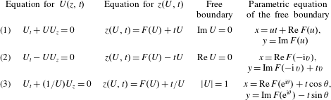
Substituting (3.14) into (3.10), we obtain $C(U)=U$. Thus, to find the complex velocity, we have to solve the Hopf equation

(3.16)$$\begin{eqnarray}U_{t}+UU_{z}=0.\end{eqnarray}$$

It should be noted that the free boundaries (3.15) are simultaneously lines of zero acceleration. Such lines, which move and become deformed with time, are found by solving the system

$$\begin{eqnarray}\frac{\text{d}u}{\text{d}t}=0,\quad \frac{\text{d}v}{\text{d}t}=0,\end{eqnarray}$$

which is rewritten in the complex form with allowance for the Cauchy–Riemann conditions (2.2) as

$$\begin{eqnarray}\displaystyle 0 & = & \displaystyle \frac{\text{d}U}{\text{d}t}=u_{t}+uu_{x}+vu_{y}-\text{i}(v_{t}+uv_{x}+vv_{y})\nonumber\\ \displaystyle & = & \displaystyle (u_{t}-\text{i}v_{t})+(u+\text{i}v)(u_{x}-\text{i}v_{x})=U_{t}+\overline{U}U_{z}=0.\nonumber\end{eqnarray}$$

Thus, to find the lines of zero acceleration on solutions of the Hopf equation, we have to solve the system

$$\begin{eqnarray}U_{t}+UU_{z}=0,\quad U_{t}+\overline{U}U_{z}=0.\end{eqnarray}$$

Subtracting the second equation from the first one, we obtain the equality $v\cdot U_{z}=0$. The second term here is equal to zero only for degenerate cases, where the velocity is independent of coordinates. Eliminating these cases, we can put forward the following statement: if the complex velocity $U(z,t)$ satisfies the Hopf equation (3.16), then $v(x,y,t)=0$ yields the free boundary with zero acceleration.

Method 2. The case with $P=-u^{2}$ is studied in a similar manner. The following statement is put forward here: if the complex velocity $U(z,t)$ satisfies the equation

$$\begin{eqnarray}U_{t}-UU_{z}=0,\end{eqnarray}$$

then the equation $u(x,y,t)=0$ yields the free boundary with zero acceleration.

Method 3. Let us apply the formulas $u=q\cos \unicode[STIX]{x1D703}$, $v=q\sin \unicode[STIX]{x1D703}$ to pass from the rectangular coordinates $u,v$ to the polar coordinates $q,\unicode[STIX]{x1D703}$. Here $q=\sqrt{u^{2}+v^{2}}$ is the absolute value of velocity. Let us consider the one-dimensional case $P=P(q)$. For this case, the Poisson equation (3.9) is written in the form

(3.17)$$\begin{eqnarray}\frac{1}{q}\frac{\unicode[STIX]{x2202}}{\unicode[STIX]{x2202}q}\left(q\frac{\unicode[STIX]{x2202}P}{\unicode[STIX]{x2202}q}\right)=-2.\end{eqnarray}$$

Integrating (3.17), we obtain

(3.18)$$\begin{eqnarray}q\frac{\unicode[STIX]{x2202}P}{\unicode[STIX]{x2202}q}=-q^{2}+A.\end{eqnarray}$$

There arises an arbitrary constant $A$ here. One more constant $q_{0}$ arises after repeated integration of (3.18). Thus, we have

(3.19)$$\begin{eqnarray}P=\frac{1}{2}\left[A\ln \frac{q^{2}}{q_{0}^{2}}-(q^{2}-q_{0}^{2})\right].\end{eqnarray}$$

It is seen that the condition of constant pressure is satisfied in the hodograph plane on the circumference $q=q_{0}$. Let us choose the constant $A$ so that the kinematic condition is also satisfied on this circumference. Taking the derivative of (3.19) with respect to time, we obtain

$$\begin{eqnarray}\frac{\text{d}P}{\text{d}t}=\left(\frac{A}{q}-q\right)\frac{\text{d}q}{\text{d}t}.\end{eqnarray}$$

This quantity should be equal to zero at $q=q_{0}$. Therefore, we have $A=q_{0}^{2}$. Thus, the pressure is determined by the formula

(3.20)$$\begin{eqnarray}P(u,v)=\frac{1}{2}\left[q_{0}^{2}\ln \frac{u^{2}+v^{2}}{q_{0}^{2}}-(u^{2}+v^{2}-q_{0}^{2})\right].\end{eqnarray}$$

The circumference

(3.21)$$\begin{eqnarray}u^{2}+v^{2}=q_{0}^{2}\end{eqnarray}$$

in the complex velocity plane corresponds to the free boundary.

Substituting (3.20) into (3.10), we obtain $C(U)=q_{0}^{2}/U$. Thus, to find the complex velocity $U(z,t)$, we have to solve the equation

(3.22)$$\begin{eqnarray}U_{t}+\frac{q_{0}^{2}}{U}U_{z}=0.\end{eqnarray}$$

It is seen from this equation that the value of $q_{0}$ can be set to unity without loss of generality by re-denoting the time $q_{0}^{2}\,t\rightarrow t$.

In this case, the zero acceleration lines can be found by solving the system

$$\begin{eqnarray}U_{t}+\frac{1}{U}U_{z}=0,\quad U_{t}+\overline{U}U_{z}=0.\end{eqnarray}$$

Subtracting one equation from the other, we obtain the equality $(1/U-\overline{U})U_{z}=0$, which yields the corollary $|U|=1$ coinciding with (3.21) (at $q_{0}=1$). Thus, we can put forward the following statement: if the complex velocity $U(z,t)$ satisfies the equation $U_{t}+(1/U)U_{z}=0$, then the equation $u(x,y,t)^{2}+v(x,y,t)^{2}=1$ describes the free boundary with zero acceleration.

The zero value of acceleration means that each fluid particle on the free boundary moves with a constant velocity. This actually means that the fluid occupies a fixed domain in the plane $U$. Therefore, it seems natural to exchange the places of dependent and independent variables. Instead of the function $U(z,t)$, we use a new unknown function $z(U,t)$. Using the formulas relating the derivatives

(3.23a,b)$$\begin{eqnarray}\frac{\unicode[STIX]{x2202}U}{\unicode[STIX]{x2202}z}=\left(\frac{\unicode[STIX]{x2202}z}{\unicode[STIX]{x2202}U}\right)^{-1},\quad \frac{\unicode[STIX]{x2202}U}{\unicode[STIX]{x2202}t}=-\frac{\unicode[STIX]{x2202}z}{\unicode[STIX]{x2202}t}\cdot \left(\frac{\unicode[STIX]{x2202}z}{\unicode[STIX]{x2202}U}\right)^{-1},\end{eqnarray}$$

and substituting them into the Hopf equation (3.16), we obtain a new equation $\unicode[STIX]{x2202}z/\unicode[STIX]{x2202}t=U$, which is easily integrable:

(3.24)$$\begin{eqnarray}z(U,t)=F(U)+tU.\end{eqnarray}$$

There arises an arbitrary analytical function $F(U)$, which defines the initial conditions at $t=0$. As condition (3.15) is satisfied on the free boundary, we can obtain the free boundary equation by substituting the equality $U=u$ into (3.24); the resultant equation parametrically depends on the real parameter $u$.

Equations and their solutions for other situations considered in the paper were obtained in a similar manner. They are presented in table 1.

Table 1.

Three methods of free boundary construction.

After finding the free boundary, we have to decide on which side of this boundary the fluid is located. The function $U(z,t)$ should be a holomorphic function in the domain occupied by the fluid; therefore, the singularities found from the equation

(3.25)$$\begin{eqnarray}\unicode[STIX]{x2202}z/\unicode[STIX]{x2202}U=0\end{eqnarray}$$

should be outside the fluid, though sources, sinks, dipoles and point vortices located inside the fluid may have certain physical meaning in some cases.

It is also desirable to draw the Riemann surface for the function $U(z,t)$. This will help us to avoid errors associated with false free surfaces or false singularities in situations where the fluid is located on one sheet of the Riemann surface, whereas the free boundaries or singularities are located on the other sheet of this surface.

4 Flows with formation of a cuspidal point on the free boundary

Let us consider an example of the flow with the use of the Hopf equation (3.16). In this case, we have to look at the first row of table 1. Let

(4.1)$$\begin{eqnarray}F(U)=1/(U+\text{i}).\end{eqnarray}$$

In this case, equation (3.24) takes the form

(4.2)$$\begin{eqnarray}tU^{2}+U(\text{i}t-z)+(1-\text{i}z)=0.\end{eqnarray}$$

Solving this quadratic equation, we find the complex velocity

(4.3)$$\begin{eqnarray}U(z,t)=\frac{z-\text{i}t\pm \sqrt{z^{2}+2\text{i}tz-(4t+t^{2})}}{2t}.\end{eqnarray}$$

Equating the radicand to zero, we find two singular points of branching

(4.4a,b)$$\begin{eqnarray}z_{0}(t)=-\text{i}(t+2\sqrt{-t}),\quad z_{1}(t)=-\text{i}(t-2\sqrt{-t}).\end{eqnarray}$$

We consider only the negative time $t<0$. Then singularities (4.4) are purely imaginary. With a change in $t$, they will move along the imaginary axis $y$.

On the free boundary, we have $U=u$; therefore, taking the real and imaginary parts of (4.2), we obtain

$$\begin{eqnarray}x=ut+\frac{u}{1+u^{2}},\quad y=-\frac{1}{1+u^{2}}.\end{eqnarray}$$

Eliminating $u$, we find the free boundary equation in the explicit form

(4.5)$$\begin{eqnarray}x^{2}=-(1+y)(y-t)^{2}/y.\end{eqnarray}$$

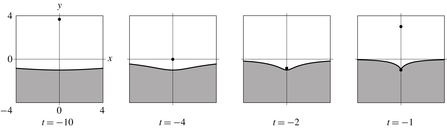
Figure 1 shows the free boundary (4.5) and the positions of the singularities for four time instants. At $t=-1$, one of the singularities reaches the free surface. At this time, the singularities are located at the points $z_{0}(-1)=-\text{i}$, $z_{1}(-1)=3\text{i}$, and the free boundary equation takes the form $x^{2}=-(1+y)^{3}/y$.

Figure 1.

Flow pattern for the first method of solution construction corresponding to formula (4.1). At large negative times $t$, two singularities $z_{0}(t)$ and $z_{1}(t)$ (see formulas (4.4)) are located at infinity outside the fluid, and the fluid occupies the lower half-plane $y\leqslant -1$. As the time progresses, the marked singularities move along the imaginary axis and approach the fluid. At $t=-1$, one of the singular points $z_{0}(t)$ reaches the free boundary. It is not clear whether the solution can be continued at $t>-1$ and how this can be done.

5 Behaviour of the free boundary approached by the singularity

To understand the mechanism of singularity formation on the fluid surface, it is important to study the motion of singular points where the analyticity of the complex velocity $U(z,t)$ is violated in the plane $z$. It should be noted that there is a certain universal law of the free boundary behaviour when the singularity closely approaches the free boundary for flows determined by the Hopf equation. Let us check this asymptotic law by an example of the exact solution considered above. Let us compare the exact formula for the free boundary (4.5) with the approximate formula (Zubarev & Karabut Reference Zubarev and Karabut2018). Let $z_{0}(t)$ be the coordinate of the singular point and $U_{0}(t)$ be the complex velocity at this point. In other words, $U_{0}(t)=U(z_{0}(t),t)$. It was shown (Zubarev & Karabut Reference Zubarev and Karabut2018) that the following equality is satisfied if the complex velocity satisfies the Hopf equation:

(5.1)$$\begin{eqnarray}U_{0}=\dot{z_{0}}.\end{eqnarray}$$

It should be noted that equality (5.1), generally speaking, does not mean that the velocity of the singular point coincides with the fluid velocity at this point. Indeed, separating the real and imaginary parts in (5.1), we obtain two equalities:

(5.2a,b)$$\begin{eqnarray}\dot{x_{0}}=u_{0},\quad \dot{y_{0}}=-v_{0}.\end{eqnarray}$$

The first equality in (5.2) shows that the singular point velocity coincides with the fluid velocity in the $x$ direction. The second equality means that these velocities have different signs in the $y$ direction. Nevertheless, by virtue of (3.15), the velocities in the $y$ direction are close to zero near the free boundary; therefore, the fluid velocity and the singular point velocity are close to each other. Thus, the following statement can be formulated: if the singularity is located close to the free boundary, it moves with a velocity close to the fluid velocity. Therefore, the following formula is valid:

(5.3)$$\begin{eqnarray}U(z,t)\approx {\dot{z}}_{0}.\end{eqnarray}$$

A more exact formula than (5.3) was derived by Zubarev & Karabut (Reference Zubarev and Karabut2018). If degenerate cases are omitted, the vicinity of the singularity contains the following root singularity:

(5.4)$$\begin{eqnarray}U(z,t)\approx {\dot{z}}_{0}+\sqrt{2\ddot{z}_{0}(z_{0}-z)}.\end{eqnarray}$$

Thus, in view of (3.15), equation (5.4) leads to the following statement: if the singularity coordinate $z_{0}$, the singularity velocity ${\dot{z}}_{0}$ and singularity acceleration $\ddot{z}_{0}$ are known, if the singular point is close to the boundary and there are no other singularities nearby, then the equation for the free boundary in the vicinity of the singular point has the form

(5.5)$$\begin{eqnarray}\text{Im}\,[{\dot{z}}_{0}+\sqrt{2\ddot{z}_{0}(z_{0}-z)}]\approx 0.\end{eqnarray}$$

Let us graphically compare the approximate asymptotic formula for the free boundary (5.5) with the exact formula (4.5). By virtue of (5.5), we have

(5.6)$$\begin{eqnarray}\sqrt{2\ddot{z}_{0}(z_{0}-z)}+{\dot{z}}_{0}=a,\end{eqnarray}$$

where $a$ is a certain real parameter. Solving (5.6) with respect to $z$, we obtain

(5.7)$$\begin{eqnarray}z=z_{0}-\frac{(a-{\dot{z}}_{0})^{2}}{2\ddot{z}_{0}}.\end{eqnarray}$$

Using (4.4), we find the singularity coordinate, velocity and acceleration:

$$\begin{eqnarray}z_{0}=-\text{i}(t+2\sqrt{-t}),\quad {\dot{z}}_{0}=-\text{i}(1-1/\sqrt{-t}),\quad \ddot{z}_{0}=\frac{\text{i}}{2(-t)^{3/2}}.\end{eqnarray}$$

Substituting all these functions into (5.7) and taking the real and imaginary parts, we obtain

$$\begin{eqnarray}x=-2at(1-\sqrt{-t}),\quad y=-3\sqrt{-t}-3t+t\sqrt{-t}-a^{2}t\sqrt{-t}.\end{eqnarray}$$

Eliminating the parameter $a$, we obtain the parabola equation

(5.8)$$\begin{eqnarray}y=-3\sqrt{-t}-3t+t\sqrt{-t}-x^{2}\frac{\sqrt{-t}}{4t(1-\sqrt{-t})^{2}}.\end{eqnarray}$$

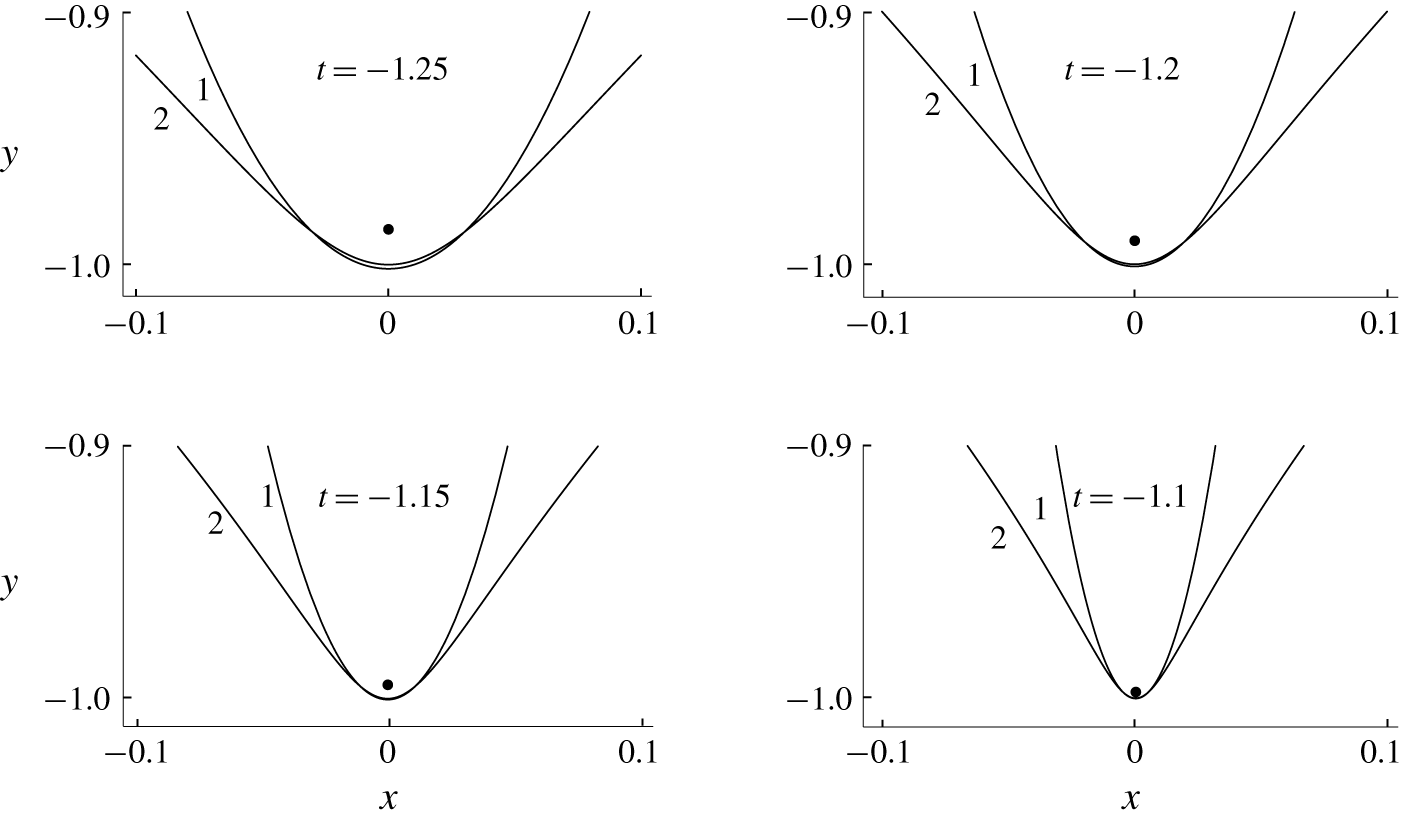
This parabola approximately describes the free boundary in the case where the singularity is located close to the boundary. Figure 2 shows a comparison between the approximate (5.8) and exact (4.5) formulas. The closer the singular point to the free boundary, the more exact the approximate formula (5.8) becomes. However, the region of closeness of (4.5) and (5.8) may be reduced as the singularity approaches the free boundary.

Figure 2.

Comparison of two equations of the free boundary for the flow described by (4.3). The evolution of this flow is shown in figure 1. Curves 2 correspond to the exact formula for the free boundary (4.5). Curves 1 are constructed with the use of the approximate formula (5.8). The marker is used to indicate the singularity reaching the free surface at $t=-1$. The figure demonstrates the change in the free boundary shape as the singularity approaches the free boundary.

6 Penetrating singularities

Let us now describe a fairly exotic scenario of the singularity behaviour near the free boundary. The hypothesis on the existence of this scenario follows from (5.3). As was noted above, the analysis of this formula shows that the fluid and singularity velocities are approximately identical if the singularity is located close to the free boundary. Therefore, there arises an idea that the region of the free boundary closely located to the approaching singularity may start to move with the velocity of the singularity itself. As a result, a long and extremely narrow channel may start to form in the fluid (we called it the penetrating singularities). Inside this channel the singularity moves without touching the channel walls.

Let us consider an example of the flow, which proves that such a scenario does exist. We search for the solution of the Hopf equation for which

$$\begin{eqnarray}F(U)=\sqrt{U-\text{i}}.\end{eqnarray}$$

Using the first row in table 1, we obtain the equation

(6.1)$$\begin{eqnarray}z-tU=\sqrt{U-\text{i}}.\end{eqnarray}$$

After squaring (6.1), we obtain the quadratic equation for finding the complex velocity

(6.2)$$\begin{eqnarray}U^{2}t^{2}-U(1+2tz)+(\text{i}+z^{2})=0.\end{eqnarray}$$

Solving (6.2), we obtain

(6.3)$$\begin{eqnarray}U(z,t)=\frac{1+2tz\pm \sqrt{1-4\text{i}t^{2}+4tz}}{2t^{2}}.\end{eqnarray}$$

Equating the radicand in (6.3) to zero, we find the only singular point

(6.4)$$\begin{eqnarray}z_{0}(t)=\text{i}t-\frac{1}{4t}.\end{eqnarray}$$

Taking the real and imaginary parts in (6.4), we see that this singular point moves along the hyperbola $y=-1/(4x)$. Substituting $U=u$ and $z=x+\text{i}y$ into (6.2) and taking the real and imaginary parts, we obtain a system of two equations. Eliminating the real parameter $u$ from this system, we obtain the free boundary equation

(6.5)$$\begin{eqnarray}x=t\left(\frac{1}{4y^{2}}-y^{2}\right)-\frac{1}{2y}.\end{eqnarray}$$

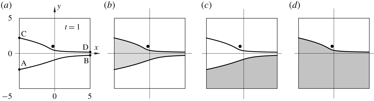
Equation (6.5) has two branches. At $t=1$, these branches are shown in figure 3(a). It should be noted that the lower branch AB is located at smaller values of $y$ than the upper branch CD. The singularity of the solution is marked in the figure. Now the following question arises: on which side of the free boundary should the fluid be placed?

Figure 3.

Two variants of fluid location. Case (c) with the fluid located below the free boundary AB is possible. Another possible case (d) is the fluid location below the free boundary CD.

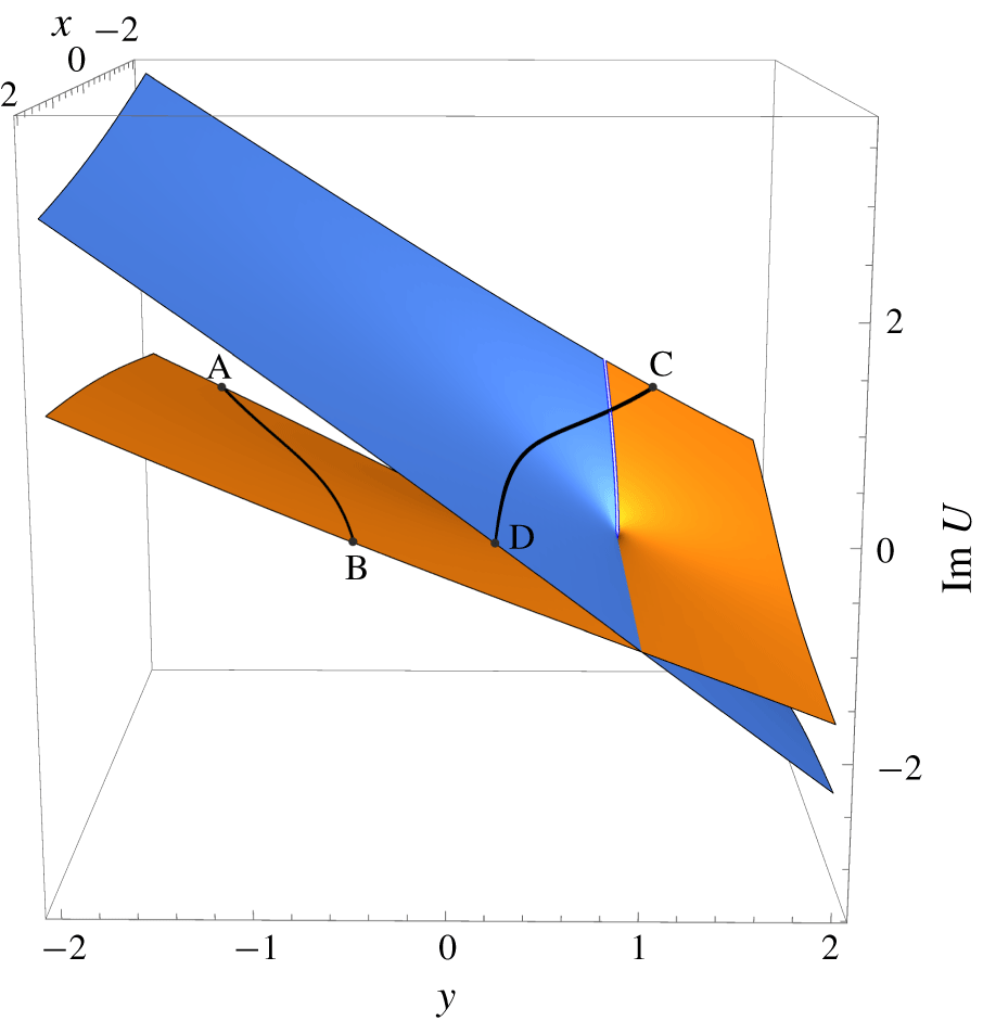
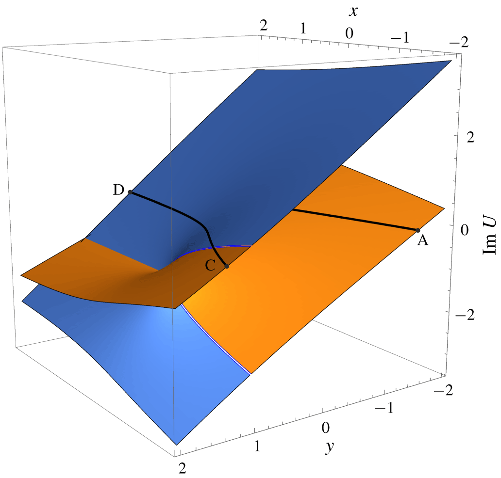
The answer to this question can be obtained using the two-sheet Riemann surface for the complex velocity $U(z,t)$, which is shown in figures 4 and 5 at two different viewing angles at a fixed time instant $t$. This Riemann surface is obtained using formula (6.3). Two horizontal axes show the real and imaginary parts of $z$, and the vertical axis presents the imaginary part of the complex velocity $\text{Im}\,U$. As the free boundary is described by the equation $\text{Im}\,U=0$, the two branches of the free boundary AB and CD shown in figure 3 rise again in figures 4 and 5 on two sheets of the Riemann surface at the places of their intersection with the horizontal plane $\text{Im}\,U=0$.

Figure 4.

Riemann surface for the complex velocity (6.3) at a certain time instant $t$. The horizontal axes show the $x$ and $y$ coordinates; the vertical axis is $\text{Im}\,U$. The curves AB and CD correspond to the free boundaries. They are obtained by intersecting the Riemann surfaces by the horizontal planes $\text{Im}\,U=0$.

Figure 5.

Riemann surface for the complex velocity. It is identical to that in figure 4, but is viewed at a different angle.

It is impossible to place the fluid above the curve CD in figure 3. Indeed, it is seen on the Riemann surface that starting from the curve CD and moving towards increasing $y$ yields a path that leads to the singular point. Therefore, the condition of holomorphicity of the complex velocity in the domain occupied by the fluid is violated.

Therefore, we have to check the possibility of fluid location only in three domains: those shown in figure 3(b–d). The case in figure 3(b) where the fluid is located between two free boundaries AB and CD is impossible. Indeed, the analysis of the Riemann surface shows that the flow simultaneously having two free boundaries AB and CD cannot exist because these boundaries are located on different sheets of the Riemann surface. More exactly, if we move over the Riemann surface starting from the line CD and moving towards negative values of $y$, we will never reach the boundary AB.

However, in such motion, it is possible to reach arbitrarily large values of $y$. This means that the fluid can be placed below the free boundary CD (figure 3d); in this case, the boundary AB will not be reached because it is located on the other sheet of the Riemann surface. This means that the case in figure 3(d) is feasible.

Similarly, starting from AB and moving towards negative values of $y$, we do not meet any obstacles, and the fluid can spread to arbitrarily large negative values of $y$. Thus, the fluid can be placed below the line AB (figure 3): the case in figure 3(c) can be realized.

Figure 6.

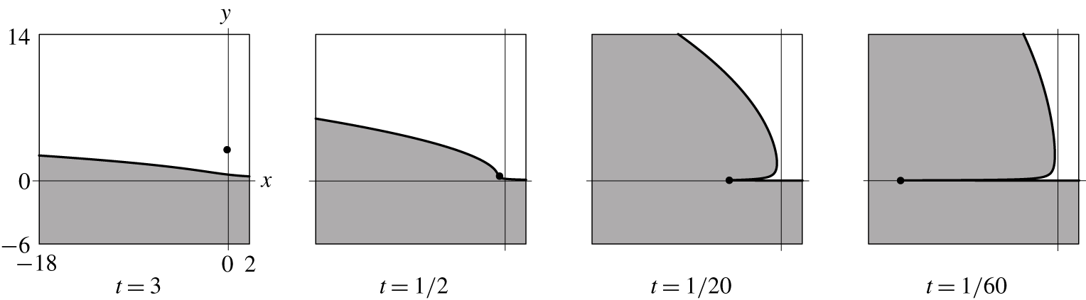
Dynamics of penetrating singularities formation. The fluid initially occupies the lower half-plane $y<0$, and the singularity moves along the $y$ axis and approaches the fluid. Then the singularity starts to penetrate into the fluid, but does not touch it anywhere. The singularity gradually changes the direction of its motion: it starts to move along the $x$ axis. As a result of singularity motion in the fluid, a penetrating singularity is formed: a long narrow channel aligned along the $x$ axis with the singularity moving inside this channel.

The time evolution of the penetrating singularity for the case in figure 3(d) is shown in figure 6. The minimum time is indicated for the rightmost panel; therefore, the flow evolution should be traced in the direction of increasing time, i.e. the panels should be viewed from right to left beginning from the rightmost panel. However, if the flow velocity vector is changed to the opposite one and time reversing is applied, i.e. $t\rightarrow -t$, then the viewing direction is also changed: now one has to consider panels from left to right.

7 Examples of flows with cavity implosion

Let us now consider another equation derived above (table 1, row 3) instead of the Hopf equation:

(7.1)$$\begin{eqnarray}U_{t}+\frac{1}{U}U_{z}=0.\end{eqnarray}$$

Changing the dependent and independent variables in (7.1) with the use of (3.23), we obtain the equation $\unicode[STIX]{x2202}z/\unicode[STIX]{x2202}t=1/U$, which is easily integrated:

(7.2)$$\begin{eqnarray}z(U,t)=F(U)+\frac{t}{U}.\end{eqnarray}$$

Figure 7.

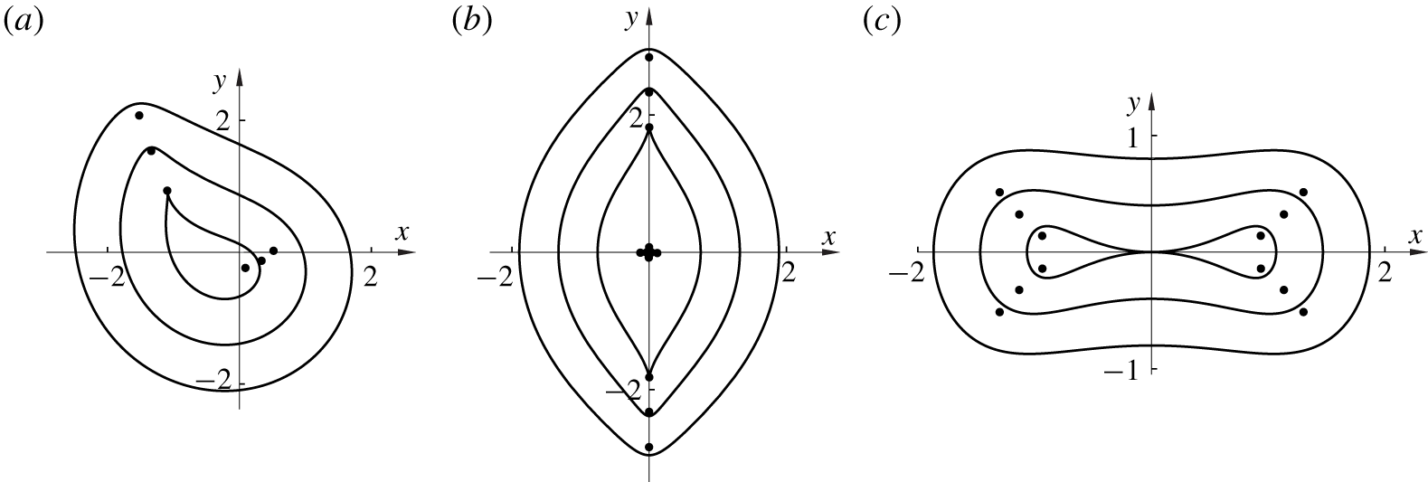
Various variants of cavity implosion. Locations of singularities (markers) and free boundary shapes for three time instants (curves). (a) Two singularities. One of them reaches the free boundary, where a cuspidal point is formed. (b) Four singularities. Two of them reach the free surface, and two cuspidal points are formed. (c) Four singularities, all outside the fluid. A collision of the free boundaries occurs, and the cavity is divided into two parts.

Prescribing the function $F(U)$, it is possible to construct multiple examples with cavity implosion. Figure 7 shows the free boundaries and locations of singularities for three variants of (7.2). Each variant is given for three time instants:

$$\begin{eqnarray}\displaystyle & \displaystyle (a)\quad z=\frac{\text{i}}{U-2\text{i}}+\frac{t}{U},\quad (t_{1}=-2.1,t_{2}=-1.4,t_{3}=-0.7). & \displaystyle \nonumber\\ \displaystyle & \displaystyle (b)\quad z=\frac{1}{U+2\text{i}}+\frac{1}{U-2\text{i}}+\frac{t}{U},\quad (t_{1}=-2.29,t_{2}=-1.72,t_{3}=-1.15). & \displaystyle \nonumber\\ \displaystyle & \displaystyle (c)\quad z=-\frac{1}{U+2\text{i}}-\frac{1}{U-2\text{i}}+\frac{t}{U},\quad (t_{1}=-1.467,t_{2}=-1.067,t_{3}=-0.667). & \displaystyle \nonumber\end{eqnarray}$$

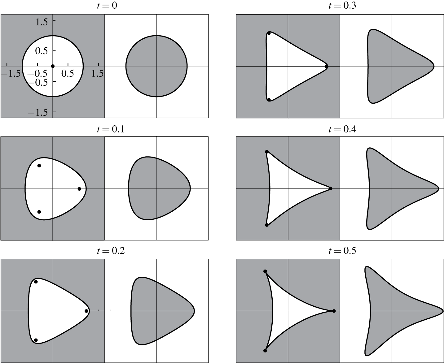
8 Two flows with a quadratic initial velocity field

Let $F(U)=\sqrt{U}$. In this case, equation (7.2) takes the form

(8.1)$$\begin{eqnarray}z=\sqrt{U}+\frac{t}{U}.\end{eqnarray}$$

It follows from here that the velocity field is initially quadratic:

(8.2)$$\begin{eqnarray}U(z,0)=z^{2}.\end{eqnarray}$$

It is also seen that the free boundary at the initial time $t=0$ is a circumference $|z|=1$. Where should be the fluid placed: inside or outside this unit circle? To answer this question, we have to know where the singularities are located.

After squaring (8.1), we see that the following cubic equation should be solved to find the complex velocity $U(z,t)$:

(8.3)$$\begin{eqnarray}U^{3}-U^{2}z^{2}+2Utz-t^{2}=0.\end{eqnarray}$$

To find the singularities of the solution, we differentiate (8.3) with respect to $U$. In view of (3.25), we obtain

(8.4)$$\begin{eqnarray}3U^{2}-2Uz^{2}+2tz=0.\end{eqnarray}$$

Eliminating the variable $U$ from the system of two equations (8.3) and (8.4), we obtain the equation for finding the coordinates of the singular points:

(8.5)$$\begin{eqnarray}27t-4z^{3}=0.\end{eqnarray}$$

There are three singularities. As follows from (8.5), one of them moves along the real axis:

(8.6)$$\begin{eqnarray}z_{0}(t)=3(t/4)^{1/3}.\end{eqnarray}$$

Two other singularities move along the rays

(8.7)$$\begin{eqnarray}z_{1,2}(t)=|z_{0}(t)|\text{e}^{\pm \text{i}2\unicode[STIX]{x03C0}/3}.\end{eqnarray}$$

At $t=0$, all three singularities are located at the origin $z=0$. As the singularities cannot be located in the fluid, the fluid should be placed outside the unit circle at the initial time.

It should be noted that the flow with a quadratic initial velocity field (8.2) and with the initial free boundary $|z|=1$ was considered in Karabut & Kuzhuget (Reference Karabut and Kuzhuget2014). In that paper, however, the fluid at the initial time occupied the interior rather than the exterior of the unit circle $|z|\leqslant 1$. Moreover, a semi-analytical rather than exact solution of the problem was obtained: power series with respect to time were used; summation of these power series was performed with the use of special-type change of variables and Pade approximants.

Figure 8.

Comparison of two flows with an identical velocity field (8.2). The study is performed for two different regions occupied by the fluid at $t=0$: either exterior or interior of the unit circle $|z|=1$. The fluid regions are marked by the grey shading. For the exterior of the circle, an exact solution is found: equation (8.1). The markers indicate three moving singularities, which migrate and reach the free boundary within a finite time. For the interior of the circle, a numerical solution is found (Karabut & Kuzhuget Reference Karabut and Kuzhuget2014). Here there are three singularities, which are always located outside the fluid.

Thus, we have two flows with similar initial data (see figure 8). Therefore, these flows have initially similar free boundaries. At later times, however, the differences in these flows become significant. The main difference is in the behaviours of singular points. For the first flow, where the fluid occupies the exterior of the cavity, it can be easily demonstrated using (8.1) that three singularities of the solution reach the free boundary at $t=1/2$. For the second (semi-analytical) solution, singular points were also investigated. In that case, three singularities were found, which were located at $t=0$ at an infinitely distant point $z=\infty$. At $t>0$, these singularities approached the free boundary, but never reached it.