1 Introduction
A major type of machine learning (or data mining) task is classification, where the algorithm learns a model for predicting the class of an object (called an instance), based on values of features describing that object. Classification algorithms are widely used in many real-world applications, for example, to determine whether or not a credit card transaction is fraudulent or to predict whether or not a patient will develop a certain disease in the future.
Many classification algorithms are available, and many new algorithms continue to be proposed, aiming at improving predictive performance. Hence, it is crucial that researchers use appropriate statistical approaches to carefully compare the predictive performance of different classification algorithms (Japkowicz & Shah Reference Japkowicz and Shah2011). Actually, in the machine learning literature, statistical significance analysis is the most used approach for determining whether or not a classification algorithm is significantly better than another (or several others), which is essential to evaluate progress in the area.
To perform such statistical analysis, a hypothesis test is used to determine if there is enough evidence to reject a certain ‘null’ hypothesis (Bussab & Morettin Reference Bussab and Morettin2010), for example, that two classifiers have the same predictive performance. However, as highlighted in Wasserstein and Lazar (Reference Wasserstein and Lazar2016), statistical significance results need to be well understood, and they should not be responsible for validating or ruling out scientific research.
Unfortunately, the p-value output by a hypothesis test is very often wrongly interpreted as the only statistical measure that should be used to evaluate the significance of a result—typically simply checking whether a condition like p-value < 0.05 is satisfied. In reality, a p-value should be just a part of a broader statistical analysis, and just comparing a p-value against a significance threshold is an over-simplified statistical approach, which may lead to discarding interesting results or to wrongly evaluate as significant a result that is not relevant in practice, as discussed below.
This problem is so worrying that the American Statistical Association (ASA) has taken a strong stand on the subject (Wasserstein & Lazer, Reference Wasserstein and Lazar2016), noting that although the p-value is a useful statistical measure, it has been abusively used and misinterpreted. Importantly, in that article, the authors advise researchers to avoid drawing scientific conclusions or making decisions based on p-values alone. According to ASA’s Executive Director Ron Wasserstein, this is the first time in 177 years, since its foundation, that ASA has made explicit recommendations on such a fundamental subject in Statistics. Wasserstein adds that ASA members are concerned that the misuse of p-values casts doubt on statistical techniques in general.
Other very important concepts, which have been most often ignored by researchers, are the power of the test and the size of the effect. The power of the test is the probability of correctly rejecting the null hypothesis when it should be rejected (Hair et al. Reference Hair, Black, Babin, Anderson and Tatham2009). Disregarding this probability can create a serious problem, especially when no statistically significant differences are obtained and the investigation is terminated. The size of the effect, on the other hand, measures the strength of the result, and ignoring this measure risks highly rating an unimportant result or disregarding a result that could be relevant.
It is worth noting that concerns with these issues are present in several areas. For example, in Medicine, in Sullivan and Feinn (Reference Sullivan and Feinn2012), it is noted that the p-value is dependent on the size of the sample. With a sufficiently large sample, a statistical test will almost always demonstrate a significant difference unless there is no effect, that is, when the effect size is exactly zero. It is also argued that very small differences are often unimportant, even if significant. Thus, for a better understanding of the results, one should report not only p-values but also effect sizes.
A particularly interesting example of the sample size problem is presented in Sullivan and Feinn (Reference Sullivan and Feinn2012): a study of the use of aspirin to prevent myocardial infarction, done in more than 22 000 individuals over a period of approximately 5 years, showed that aspirin was associated with a highly significant reduction in the number of cases in myocardial infarction based on a very small p-value (p-value < 0.00001). The study was terminated early because of the supposedly conclusive evidence and aspirin was recommended for this prevention. However, at a later time, it was found that the effect size was extremely small. Thus, many people who were advised to take aspirin experienced no benefit at all and were still at risk of adverse effects. Other studies have found even smaller effects and the recommendation to use aspirin has since been modified.
As further examples, both authors in Biology (Nakagawa & Cuthill Reference Nakagawa and Cuthill2007) and authors in Sport Sciences (Tomczak & Tomczak Reference Tomczak and Tomczak2014) have noted that, although the use of significance tests is by far the predominant approach for statistical analysis of experimental results in their disciplines, such tests have the serious limitation of not providing important information about the size of an effect, and both authors recommend the use of statistical measures of effect size.
In addition, in Psychology, it is reported in Kline (Reference Kline2004) that data analysis practices are changing, as shown by the increasing number of journals that require information about the size of the effect. In this work, a statement by Gene Glass, a statistician who works in Educational Psychology and Social Sciences, is highlighted: ‘Statistical significance is least relevant to results. It is important that the results in terms of magnitude are presented because one should not only inform that a treatment affects people, but how much it affects them’.
As seen above, studies from various fields are recommending that authors report some measure of effect size and, increasingly, this approach has been encouraged, in some cases even required, by the editors of scientific journals.
In this work, we surveyed all 69 articles published in the Machine Learning journal in 2017 (ML Journal Reference Journal2017). Out of these, 17 articles used a classification method, but 8 of them did not use any statistical hypothesis test (Cousins & Taylor Reference Cousins and Taylor2017; Huang & Lin Reference Huang and Lin2017; Kotłowski & Dembczyński Reference Kotłowski and Dembczyński2017; Mena et al. Reference Mena, Montañés, Quevedo and Del Coz2017; Kim & Oh, Reference Kim and Oh2017; du Plessis et al. Reference du Plessis, Niu and Sugiyama2017; Suzumura et al. Reference Suzumura, Ogawa, Sugiyama, Karasuyama and Takeuchi2017; Xuan et al. Reference Xuan, Lu, Zhang, Da Xu and Luo2017). In the other nine articles that used at least one hypothesis test (Bertsimas & Dunn Reference Bertsimas and Dunn2017; Cardoso et al. Reference Cardoso, Gama and França2017; Gomes et al. Reference Gomes, Bifet, Read, Barddal, Enembreck, Pfharinger, Holmes and Abdessalem2017; Júnior et al. Reference Júnior, de Souza, Werneck, Stein, Pazinato, de Almeida, Penatti, Torres and Rocha2017; Osojnik et al. Reference Osojnik, Panov and Džeroski2017; Wu & Lin Reference Wu and Lin2017; Yu & Zhang Reference Yu and Zhang2017; Krijthe & Loog Reference Krijthe and Loog2017; Zaidi et al. Reference Zaidi, Webb, Carman, Petitjean, Buntine, Hynes and De Sterck2017), we noted the statistical analysis focused on simply checking the condition p-value < 0.05, that is, no article reported a measure of the effect size or the power of the test.
Out of these nine articles, three of them (Júnior et al. Reference Júnior, de Souza, Werneck, Stein, Pazinato, de Almeida, Penatti, Torres and Rocha2017; Krijthe & Loog Reference Krijthe and Loog2017; Cardoso et al. Reference Cardoso, Gama and França2017) used the Wilcoxon test and three others (Osojnik et al. Reference Osojnik, Panov and Džeroski2017; Gomes et al. Reference Gomes, Bifet, Read, Barddal, Enembreck, Pfharinger, Holmes and Abdessalem2017; Zaidi et al. Reference Zaidi, Webb, Carman, Petitjean, Buntine, Hynes and De Sterck2017) used the Friedman test with the Nemenyi test. One article (Yu & Zhang Reference Yu and Zhang2017) used the Student’s t-test and another (Wu & Lin Reference Wu and Lin2017) used the Student’s t-test with the Friedman test. Another article (Bertsimas & Dunn Reference Bertsimas and Dunn2017) reports an ‘orphan’ p-value, since the hypothesis test carried out was not reported.
This survey also identified other problems. Four articles (Júnior et al. Reference Júnior, de Souza, Werneck, Stein, Pazinato, de Almeida, Penatti, Torres and Rocha2017; Krijthe & Loog Reference Krijthe and Loog2017; Gomes et al. Reference Gomes, Bifet, Read, Barddal, Enembreck, Pfharinger, Holmes and Abdessalem2017; Cardoso et al. Reference Cardoso, Gama and França2017) did not report the computed p-values, reporting only the performed test, the significance level and whether or not the p-value was significant. Two articles (Yu & Zhang Reference Yu and Zhang2017; Osojnik et al. Reference Osojnik, Panov and Džeroski2017) reported the critical values rather than the p-values. Finally, only two articles (Wu & Lin Reference Wu and Lin2017; Zaidi et al. Reference Zaidi, Webb, Carman, Petitjean, Buntine, Hynes and De Sterck2017) reported the computed p-values together with the performed test and the significance level used.
In view of this scenario, this work discusses in detail why the p-value, alone, is not sufficient to perform well the comparison of classifiers. We also discuss measures that add valuable information to statistical analyses, namely the effect size and the power of the test. In order to highlight the importance of these measures, we have carried out experiments with four very popular classifiers: Random Forest (Breiman Reference Breiman2001), Support Vector Machine (SVM) (Hearst et al. Reference Hearst, Dumais, Osuna, Platt and Scholkopf1998), k-Nearest Neighbor (NN) (Cover & Hart Reference Cover and Hart1967) and Naive Bayes (NB) (Langley et al. Reference Langley, Iba and Thompson1992), using 50 datasets freely available from the well-known UCI repository (Dheeru & Taniskidou Reference Dheeru and Taniskidou2017). The statistical significance of the difference between the accuracies of the classifiers was verified by means of the Student’s t-test and the Wilcoxon test, together with the calculation of the effect size and the power of the test. We chose those two tests because they are reasonably popular representatives of two different approaches for statistical significance testing, namely the parametric approach (for the Student’s t-test) and the non-parametric approach (for the Wilcoxon test).
In the conducted studies, we observed, as expected, that in many cases the three measures (p-value, effect size and power of the test) are concordant. For example, a p-value evidencing statistical significance with a high effect size and also a high power of the test. However, we have also found several cases where these measures are discordant, called here ‘special cases’, which will be highlighted in this article.
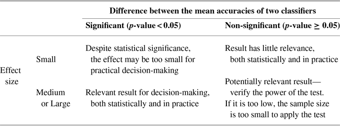
More precisely, cases where the accuracy difference is statistically significant, but with a low effect size, require caution when drawing conclusions, since there is a risk of valuing a result that is not of real importance (like the above example of aspirin’s extremely small effect on myocardial infarction prevention). However, the opposite cases, with a relevant effect size but no statistical significance on the accuracy differences, could lead to miss interesting results if the conclusion was drawn based only on the p-value. In some cases, the power of the test may help to justify why the p-value and effect size are disagreeing, in which case the use of the test may be sub-optimal. As, for example, when the sample is too small and not sufficient to detect a significant result.
It should be noted that recently Benavoli et al. (Reference Benavoli, Corani, Demšar and Zaffalon2017) have also made a strong criticism about the traditional use of p-values for statistical significance analysis. However, their work has a different focus than this current work: their article argues that the null hypothesis significance test framework should be abandoned, replaced by a Bayesian framework, whilst in this work we keep that framework and focus on extending (complementing) the traditional use of p-values with measures of effect size and the power of the test.
Before proceeding, it is important to clarify the terminology used in this work. When we refer to the three measures (p-value, effect size and test power) as concordant or discordant, we do not mean agreement in the mathematical sense, since these measures are obviously non-commensurate—that is, they measure different aspects of the result or the use of a statistical significance test, and therefore they are not directly mathematically comparable. We refer instead to the agreement or disagreement between the practical conclusions that could be drawn by the user by observing the values of the p-value, effect size and test power.
This article is organized as follows. In Section 2, the theoretical background on statistical hypothesis tests and effect size measures is reviewed. We focus on the Student’s t-test and the Wilcoxon test for matched data and their respective effect size measures. In Section 3, which is based on the preliminary results reported in Neumann et al. (Reference Neumann, Plastino, Junior and Freitas2018), two case studies are presented, one for Student’s t-test and one for the Wilcoxon test, where the p-value and the effect size disagree, called special cases. In Section 4, a larger study is carried out, considering 4 classifiers and 50 datasets, comparing the results by each of the above two tests. It will be noted that special cases occur frequently in those experiments. Finally, in Section 5, the conclusions and possible directions for future work are presented.
2 Background on statistical significance analysis
2.1 Hypothesis tests
Usually, we use inferential statistics because it allows us to measure behavior in samples to learn more about the behavior in populations that are often too large or inaccessible. The most used approach where we select samples to learn more about characteristics in a given population is called hypothesis tests.
A hypothesis test is a very efficient method for testing a claim or hypothesis about an unknown parameter in a population, using data measured in a sample. The procedure involves two hypotheses, called the null (conservative) and the alternative (innovative) hypotheses. For instance, consider two classification algorithms A and B, and the variables X and Y representing, respectively, the accuracy of A and the accuracy of B obtained using specific training and test datasets. The accuracy of a classification algorithm, built on a training dataset, is defined as the ratio of the number of correctly classified instances in the test set over the total number of instances in that test dataset (i.e., all classified instances). Consider then the statement that the population means of the accuracies of two classification algorithms A and B are equal, and another statement that their population means are different. In this scenario, the first one is the null hypothesis and the second one is the alternative hypothesis, mathematically defined by:
 \begin{eqnarray} \left\{\begin{array}{rr}H_0: & \mu_X = \mu_Y\\H_1: & \mu_X \neq \mu_Y\end{array}\right .{ \quad and\quad }\left\{\begin{array}{rr}H_0: & \mu_D=0\\H_1: & \mu_D \neq 0\end{array}\right .\end{eqnarray}
where
 $\mu_X$
and
 $\mu_Y$
are the population means of the accuracies of classification algorithms A and B, respectively. In this scenario, the samples are dependent (paired) and we could define
 $D=X-Y$
, that is, D represents the difference between the accuracies of the two classification algorithms,
 $\mu_D$
is the difference between the population means of the classifiers A’s and B’s accuracies and
 $\overline{D}$
is the estimator of this parameter.
At the end of the procedure, we decide whether or not to reject the null hypothesis, and this decision can be correct or incorrect. There are two types of errors in hypothesis tests: Type I and Type II errors. A Type I error consists in rejecting a null hypothesis that is actually true. It is important to emphasize that the probability of this type of error (
 $\alpha$
) is determined by the researcher and stated as the level of significance for a hypothesis test. A Type II error consists in not rejecting a null hypothesis that is actually false, with an associated probability (
 $\beta$
). That is, these probabilities are defined as follows:
 \begin{equation}\alpha = P(\text{Type I error}) = P(\text{reject }H_0 | H_0\text{ is true}), \qquad\quad\ \end{equation}
 \begin{equation}\beta = P(\text{Type II error}) = P(\text{do not reject }H_0 | H_0\text{ is false}). \end{equation}
If
 $H_0$
is rejected, we are assuming
 $\mu_D \neq 0$
. Thus, there are several different values for
 $\mu_D$
, and Equation (3) can be rewritten as a function of
 $\mu_D$
:
 \begin{equation}\beta(\mu_D) = P(\text{do not reject }H_0 | \mu_D). \end{equation}
The decision could be made based on a rejection region or p-value (the most used approach). The p-value is defined as the probability of observing values of the test statistic (T) greater than the observed value (t), under the null hypothesis (Fisher Reference Fisher1925). For a one-tailed test, we can define the p-value as follows:
 \begin{eqnarray}\text{{p}-value}=P(T\geq |t| \vert H_0). \end{eqnarray}
For a two-tailed test, the p-value is given by
 $P(T \geq |t| \vert H_0)+P(T \leq -|t| \vert H_0)$
.
2.1.1 Paired Student’s t-test
The paired sample t-test, sometimes called the dependent sample t-test, is a statistical procedure used to determine whether the mean difference between two sets (
 $\mu_D$
) of observations is zero. In a paired sample t-test, each subject or entity is measured twice, resulting in pairs of observations.
As a parametric procedure, the paired sample t-test makes several assumptions. Although t-tests are quite robust, it is good practice to evaluate the degree of deviation from these assumptions in order to assess the quality of the results. These assumptions include that the dependent variable should be approximately normally distributed. To test this assumption, a variety of methods are available, including graphic inspections (histogram and qqplot) or hypothesis tests such as Kolmogorov–Smirnov and Shapiro–Wilk.
In our work, to compare the accuracies of two classifiers we will use a two-tailed test and the hypotheses are defined as follows:
 \begin{eqnarray} \left\{\begin{array}{cc}H_0: & \mu_D = 0\\H_1: & \mu_D \neq 0\end{array}\right .\end{eqnarray}
The test statistic is calculated as:
 \begin{eqnarray} T=\frac{\overline{D}-\mu_D}{\sqrt{\frac{s_d^2}{n}}},\end{eqnarray}
where n is the sample size and
 $s_d^2$
is the variance of the sample differences.
Under null hypothesis, the test statistic
 \begin{equation}T \sim t_{(n-1)},\end{equation}
and the p-value will be obtained by
 \begin{eqnarray}\text{{p}-value} = P(T \geq |t||H_0) + P(T \leq -|t| |H_0) = 2 \times P(T \geq |t||H_0). \end{eqnarray}
2.1.2 Wilcoxon signed rank test
The Wilcoxon signed rank test is a non-parametric hypothesis test used to compare two related samples. It can be used as an alternative to the paired Student’s t-test when the population is not normally distributed.
The hypotheses can be written in terms of the median (
 $\delta_D$
) as follows:
 \begin{eqnarray} \left\{\begin{array}{cc}H_0: & \delta_D = 0\\H_1: & \delta_D \neq 0\end{array}\right .\end{eqnarray}
To compute the test statistic W, first we assign a rank to each absolute value of the difference between the classifiers’ accuracies, where the smallest difference gets rank 1, the second smallest gets rank 2, etc. Each rank is assigned the sign of its corresponding difference, to identify positive and negative ranks. Then, the test statistic for the Wilcoxon signed rank test is given by
 \begin{equation*}W = \min\{W^+,W^-\},\end{equation*}
where
 $W^+$
is the sum of the positive ranks and
 $W^-$
is the sum of the negative ranks. If the null hypothesis
 $H_0$
is true, each rank has the same probability of being a positive or negative one, that is,
 $W^+$
and
 $W^-$
would be similar. Hence, small values of W would lead to the rejection of
 $H_0$
. The decision can also be made based on the p-value:
 \begin{equation}p-value=P(W\leq w \mid H_0).\end{equation}
The p-value in Equation (11) could be obtained from tables for small samples and W could be approximated by a normal distribution for large samples.
2.2 The power of a hypothesis test
An important concept in the context of hypothesis tests is the power of the test, which is the probability of rejecting the null hypothesis when it is really false. Some authors state that the power of a test should be higher than 80% to be acceptable (Cohen Reference Cohen1988). By definition, as shown in Equation (4), the power is related to the probability of a Type II error by complementarity, and thus the power is a function of
 $\mu_D$
that could be written as:
 \begin{eqnarray}\pi(\mu_D)= 1- \beta (\mu_D) = P({reject }H_0 \mid \mu_D). \end{eqnarray}
Considering the two-tailed t-test, the power function will be defined by
 \begin{eqnarray}\pi(\mu_D) = P \left( T > \left( \frac{v_1-\mu_D}{\frac{s_d}{\sqrt{n}}} \right) \mid T \sim t_{(n-1)} \right) + P \left( T
< \left( \frac{v_2-\mu_D}{\frac{s_d}{\sqrt{n}}} \right) \mid T \sim t_{(n-1)} \right)\end{eqnarray}
where
 $v_1$
and
 $v_2$
are the limits from the rejection region. Under the null hypothesis defined by Equation (6), Equation (13) can be simplified to
 \begin{eqnarray}\pi(\mu_D) = 2 \times P \left( T > \left( \frac{v_1-\mu_D}{\frac{s_d}{\sqrt{n}}} \right) \mid T \sim t_{(n-1)} \right)\end{eqnarray}
In this work, the power of the Wilcoxon signed rank test will be computed via simulations based on samples of normal distributions, following Barros and Mazucheli (Reference Barros and Mazucheli2005). The parameters of these distributions used in the simulations are the means and variances obtained from the samples used in the hypothesis test. To compute the power, we generate 1000 paired samples with the same size of the sample size used in the test. The power function of the Wilcoxon signed rank test, considering the difference observed between the samples, will be the proportion of times that the Wilcoxon signed rank test rejects the null hypothesis.
2.3 Effect sizes
An inferential test may be statistically significant, but this does not necessarily indicate how large the effect is. The effect size is a simple way of quantifying the effective difference between two groups, which has many advantages over the use of tests of statistical significance alone (Cohen Reference Cohen1988). In particular, the effect size emphasizes the size of the difference rather than confounding this with the sample size.
Cohen’s d measures the effect size for the paired t-test (Cohen Reference Cohen1988):
 \begin{eqnarray}d'cohen = \left| \frac{\overline{D}}{s_D} \right| = \left| \frac{\frac{\overline{D}}{\sqrt{n}}}{\frac{s_D}{\sqrt{n}}}\right| = \left| \frac{t}{\sqrt{n}} \right| ,\end{eqnarray}
where t is the value observed for the test statistic and n is the sample size (number of pairs). Cohen (Reference Cohen1988) established cutoffs for interpreting the values of Cohen’s d measure, as shown in Table 1.
Values for the interpretation of Cohen’s d measure of effect size

For the Wilcoxon signed rank test, the effect size r will calculated as:
 \begin{eqnarray}r= \frac{z}{\sqrt{N}},\end{eqnarray}
where N is the sum of the sample size (i.e., twice the number of pairs) and z is the value observed for the patronized test statistic W. Cohen (Reference Cohen1988) also established cutoffs for r, as shown in Table 2.
Values for the interpretation of the measure r of effect size

3 Is p-value < 0.05 enough?: Two case studies
This section shows, using real-world case studies, that just checking the condition p-value < 0.05 is not enough for a sound statistical analysis and can mislead researchers to ignore relevant results or to value a non-relevant result. In these case studies, the p-value and effect size measures led to discordant conclusions, and it is shown how the calculation of the power of the test can help explain such discordance. This section is based on preliminary results reported in Neumann et al. (Reference Neumann, Plastino, Junior and Freitas2018).
3.1 Case study with the Student’s t-test
We explore a case study where the result of the Student’s t-test with matched pairs indicates no statistical significance, but the effect has a medium size. The goal is to determine whether or not the predictive accuracies of the 1-NN and 3-NN classifiers are significantly different on the dataset Mammographic Mass, obtained from the well-known UCI repository. A classifier’s predictive accuracy was computed using the simple accuracy measure, which is the proportion of correctly classified testing instances (unseen during training) over the number of classified testing instances.
The experiments were performed using the popular WEKA tool (Witten et al. Reference Witten, Frank, Hall and Pal2016), using 10-fold cross-validation. Hence, there are 10 pairs of accuracies for 1-NN and 3-NN, justifying the use of a matched-pairs hypothesis test. The paired accuracies for each cross-validation fold (f1,…,f10) are shown in Table 3.
Accuracy (%) obtained in each cross-validation fold for each classifier

3.1.1 Conclusion drawn from the p-value only
Let X and Y be the samples of accuracies obtained by 1-NN and 3-NN, respectively, and let (
 $x_i$
,
 $y_i$
),
 $1\leq i\leq 10$
, be the 10 pairs of accuracies obtained by 1-NN and 3-NN in the 10-fold cross-validation. In addition, let
 $d_i=x_i-y_i$
,
 $1\leq i\leq 10$
, be the corresponding differences between the paired accuracies. First, we need to verify the assumption of normality of the distributions of X and Y required for applying the matched pairs t-test. This assumption is checked by using the Kolmogorov–Smirnov test for each distribution, with the following null (
 $H_0$
) and alternative (
 $H_1$
) hypothesis for each classifier.
 \begin{eqnarray} \left\{\begin{array}{cl}H_0: & {The accuracies have normal distribution}\\H_1: & {The accuracies do not have normal distribution}\end{array}\right .\end{eqnarray}
Clearly, accuracy values are limited to be between 0 and 1, so they are not strictly normally distributed. Despite this, the normality test is performed, because the distribution of X or Y can be close to the normal one (it can be symmetric with the same mean and median), in which case the use of the t-test would be acceptable.
The results of the Kolmogorov–Smirnov test at the 5% significance level are that the null hypothesis (representing a normal distribution) cannot be rejected, with p-values of
 $0.68$
and
 $0.83$
for the accuracy distributions of 1-NN and 3-NN, respectively. Hence, we proceed by applying the t-test (also at the 5% significance level) for the matched pairs with unknown variances.
We use a two-sided t-test, since our goal is to detect whether or not a classifier is more accurate than another, regardless of which classifier is better. Hence, the null hypothesis is that the population mean of the 1-NN’s accuracies is equal to the population mean of the 3-NN’s accuracies. The alternative hypothesis is that these two population means are different. That is:
 \begin{eqnarray} \left\{\begin{array}{cc}H_0: & \mu_D = 0, \\H_1: & \mu_D \neq 0,\end{array}\right .\end{eqnarray}
where
 $\mu_D$
is the difference between the population means of the 1-NN’s and 3-NN’s accuracies.
The t-test statistic is calculated as defined in Equation (7), so in our case this statistic is calculated as follows, where
 $\overline{d}=-2.08$
is the observed difference in the sample accuracies:
 \begin{equation}t=\frac{\overline{d}-0}{\frac{s_d}{\sqrt{n}}} = \frac{-2.08}{\frac{2.95}{\sqrt{10}}} = -2.24,\end{equation}
since
 \begin{equation}s_d=\sqrt{\frac{\sum_{i=1}^n(d_{i}-\overline{d})^2}{n-1}} = \sqrt{\frac{78.12}{10-1}} = 2.95.\end{equation}
Using Equation (9) to calculate the p-value, we obtain
 $2 \times P(t \geq |t||H_0) = 2 \times 0.0261=0.0522$
. Since the p-value is the probability of obtaining values more extreme than the observed one when
 $H_0$
is true, we need to add up the probabilities of values more extreme than the calculated one for a t-distribution with nine degrees of freedom.
Hence, since the p-value
 $\,=0.052$
is greater than the significance level
 $\alpha=0.05$
, the result of the matched-pairs t-test does not provide evidence for rejecting the null hypothesis that the population means of the 1-NN’s and 3-NN’s accuracies are equal.
3.1.2 Interpreting effect sizes
The value of an effect size measure can complement the p-value in a significance analysis. In our above case study, the Cohen measure of effect size, defined in Section 2.3, is calculated as
 $d'cohen=\frac{|t|}{\sqrt{n}}=\frac{2.24}{\sqrt{10}}=0.71$
, where t is the t-test statistic and n is the number of matched pairs (sample size).
Table 1 shows that
 $d'cohen=0.71$
represents an effect of medium size. That is, although the t-test’s result does not indicate a significant difference between the mean accuracies of 1-NN and 3-NN, the difference between these means has medium size, indicating that the magnitude of the difference may be relevant. Hence, the p-value and the d’cohen value indicate different results. In this case, the calculation of the power of the test, discussed in the next subsection, provides additional information required for making a more principled decision.
3.1.3 Calculating the power of the test
As discussed in Section 2.2, the power of the test represents the probability of correctly rejecting
 $H_0$
, that is, the probability of concluding that a pair of classifiers have different mean accuracies, when they actually do. The power of the test is actually a function because, when
 $H_0: \mu_D = 0$
is false, we do not know the actual value of
 $\mu_D$
, we only know it is different from zero and so the power of the test is calculated for all possible values of
 $\mu_D$
.
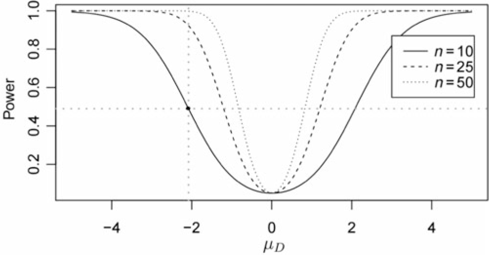
In Figure 1, the curve for
 $n=10$
represents the test power function for the possible values of the difference between the population means of the accuracies of the pair of classifiers being compared, that is, for all possible values of
 $\mu_D$
. In addition to the curve for
 $n=10$
(sample size in our case study), the figure also shows the curves representing the test power functions for two hypothetical larger sample sizes (numbers of paired accuracies),
 $n=25$
and
 $n=50$
. In the figure, the point marked in the curve for
 $n=10$
refers to the power of the test if the actual difference between the population mean accuracies was
 $-2.08$
(the observed sample difference). In this case, the power of the test (calculated via Equation (12)) is
 $0.49$
, which is the value for the point marked in the figure.
Curves for the power of the test with several n (sample size) values

That is, if the actual difference of population mean accuracies between the two classifiers is
 $-2.08$
, the probability of the test indicating that the classifiers’ mean accuracies are different (correctly rejecting
 $H_0: \mu_D = 0$
) is only 49%.
In addition, Figure 1 shows that, for a fixed
 $\mu_D$
value, the power of the test increases with the sample size (n). For instance, for
 $\mu_D=-2.08$
, when n = 10, 25, 50, the power of the test is 49%, 92% and 98%, respectively.
As discussed earlier, the t-test’s result (p-value =
 $0.052$
) did not allow us to reject the null hypothesis, so we could not conclude the population means of the 1-NN’s and 3-NN’s accuracies are different at the significance level of 5%. However, the calculated medium effect size (
 $d'cohen=0.71$
) indicates that the magnitude of that difference can be important. That is, the two measures can lead to different conclusions about the difference in the classifiers’ accuracies.
In the above case study, the power of the test (only 49%) allow us to understand why the p-value and the d’cohen measures led to different results. That is, the t-test was used despite having relatively little power for the available sample size (10 accuracy pairs). Hence, this case study shows not only the importance of considering the three measures as a whole but also the risk of making a wrong decision based on the p-value only. It also shows the drawback of using a hypothesis test without knowing its power for the available samples.
In such cases, when the effect size is potentially relevant, the researcher should not abandon the study because the result of a test with little power did not indicate statistical significance, which could lead to missing an important result.
3.2 Case study with the Wilcoxon test
In this section, we explore a case where the hypothesis test indicates statistical significance, but with a small effect size. This case study will use the matched-pairs Wilcoxon test in order to analyze the differences in the mean accuracies of 1-NN and 3-NN in another dataset from the UCI repository, viz. Wholesale3. Unlike the previous section, where 10-fold cross-validation was used, here we use 30 folds, that is, the sample size is 30.
3.2.1 Conclusion based on the p-value
Let X and Y be the samples of accuracies obtained by 1-NN and 3-NN, respectively. Consider
 $(x_1,y_1)$
,
 $(x_2,y_2)$
, …,
 $(x_{n},y_{n})$
, where
 $n=30$
, the 30 observed accuracy pairs, with corresponding differences
 $d_i=x_i-y_i$
, where
 $1\leq i\leq n$
. We will apply the two-sided, matched-pairs Wilcoxon test with the significance level of 5%, whose hypotheses are shown in Equation (21), where
 $\delta_D$
is the median of the differences between the population mean accuracies of the 1-NN and 3-NN classifiers in the Wholesale3 dataset.
 \begin{eqnarray} \left\{\begin{array}{cc}H_0: & \delta_D = 0\\H_1: & \delta_D \neq 0\end{array}\right .\end{eqnarray}
Hence, the null hypothesis is that there is no difference between the medians of the population accuracies of 1-NN and 3-NN, whilst the alternative hypothesis is that there is a difference between those medians.
First, we calculate the ranks for the absolute values of the observed accuracy differences, sorted in increasing order. The value of n is recalculated, since 13 accuracy pairs are ignored due to having a null difference, so that
 $n=17$
. The W statistic is the minimum between the sum of positive ranks and the sum of negative ranks, which in our case is the former sum, viz.:
 $W=3.5+11+15=29.5$
.
In this case, the p-value obtained with the Wilcoxon test is
 $0.025$
, which is smaller than the significance level
 $\alpha=0.05$
, so there is evidence to reject the null hypothesis. Hence, we can claim, at this significance level, that the medians of the population accuracies of 1-NN and 3-NN are significantly different.
3.2.2 Interpreting effect sizes
As noted earlier, the value of an effect size measure can complement a p-value in a significance analysis. In our case study, the effect size measure r, defined in Section 2.3, is calculated as:
 $r=\frac{|z|}{\sqrt{N}}=\frac{2.24}{\sqrt{60}}=0.28$
, where z is the Wilcoxon test statistic approximated by the normal distribution and N is the sum of the sample sizes, that is, twice the number of matched accuracy pairs (
 $N=2\times n$
).
As shown in Table 2,
 $r=0.28$
is a small effect size. Hence, the hypothesis test’s result suggests that the difference between the medians of the population accuracies of 1-NN and 3-NN is significant, but the small effect size suggests that the magnitude of this difference may not be relevant for the researcher. In this case, the p-value and the effect size measure suggest different conclusions. Again, the calculation of the power of the test, discussed in the next subsection, provides additional information required for making a more principled decision.
3.2.3 Calculating the power of the test
To use the Wilcoxon test, it is not necessary to make any assumption about the distribution of the population, since it is a non-parametric test. However, the calculation of the power of the test requires that the distribution of the accuracy differences be known, which will be obtained via simulation.
We simulated 1000 pairs of samples, each with sample size 30, randomly drawn from a normal distribution with the mean and standard deviation of the corresponding samples X and Y. For each sample pair, we applied a Wilcoxon test and then measured the proportion of significant results (where p-value < 0.05), which was
 $43.3\%$
(433 out of 1000). Hence, the power of the test (for
 $n=30$
) is
 $43.3\%$
. That is, when 1-NN and 3-NN have a median population accuracy difference of
 $-3.36$
(observed sample difference), the probability of the test indicating that the classifiers have different accuracies is about 43%.
As noted earlier, the Wilcoxon test provided evidence to reject the null hypothesis (p-value = 0.025), indicating a significant difference between the classifiers’ accuracies. However, the
 $r=0.28$
measure indicates that the effect size for that accuracy difference is small and can be a non-relevant result. Hence, the p-value and the effect size measure can lead to different conclusions.
Again, the calculation of the power of the test allows us to understand why the two measures led to different conclusions. The relatively small power of the test, 43%, when the population accuracy difference is equal to the samples accuracy difference, shows that the test has a relatively small probability of indicating that the classifiers have different accuracies when that different actually exists. That is, in this case, the Wilcoxon test was used despite its small power for this sample size. Therefore, like in the case study with the t-test, this case study shows not only the importance of calculating the three measures but also the risk of making a wrong decision based on the p-value only, and the misleading conclusion that can be drawn if the power of the test is unknown for the current sample.
4 Expanded analysis
In Section 3, we explored two cases of classifier comparison, showing that the decisions based only on the p-value could lead to misleading conclusions. We also discussed how the analysis of both effect size and power of the test can collaborate for better decisions. Such cases, where there is a disagreement between the p-value and the effect size, will henceforth be called special cases.
In this section, the previous analyses are expanded by performing an empirical study to investigate the behavior of the three measures (p-value, effect size and power of the test) in several classifier–comparison scenarios. This will show that special cases occur with a substantial frequency.
For this empirical study, we selected 50 datasets from the UCI repository. Since we use cross-validation with up to 30 folds, each selected dataset had a minimum of 300 instances, to avoid the use of very small test sets. The used datasets have from 306 to 14 980 instances, from 3 to 857 attributes and between 2 and 37 classes.
For each dataset, the following classification algorithms were applied: Random Forest with 100 trees (RF100) and 300 trees (RF300), SVM, k-NN with k=1 (1-NN) and k=3 (3-NN) and NB, in total six classifiers.
We have evaluated the following 15 pairs of classifiers: (1) RF100 and RF300; (2) RF100 and SVM; (3) RF100 and 1-NN; (4) RF100 and 3-NN; (5) RF100 and NB; (6) RF300 and SVM; (7) RF300 and 1-NN; (8) RF300 and 3-NN; (9) RF300 and NB; (10) SVM and 1-NN; (11) SVM and 3-NN; (12) SVM and NB; (13) 1-NN and 3-NN; (14) 1-NN and NB; (15) 3-NN and NB.
To expand the scope of the experiment, for each dataset, each classifier was evaluated with 10, 20 and 30 folds in the cross-validation procedure. The experiments were carried out with the Weka Tool.
Using the obtained accuracies, the Student’s t-test and the Wilcoxon test were then applied, both for paired samples. Each test was applied to every possible combination of a pair of classifiers, a dataset and a sample size. Hence, each test was executed a total of
 $15\times50\times3=2250$
times. In the conducted evaluation, apart from the p-values, the effect size and the power of the test were also calculated. These evaluations were done using the software R.
Next, Subsections 4.1 and 4.2 show the results obtained for the Student’s t-test and the Wilcoxon test, respectively.
4.1 Analysis with the Student’s t-test
In this section, we present the results obtained with the measures p-value, effect size and power of the test in the comparison of the 15 pairs of classifiers, considering 50 datasets and using the Student’s t-test.
As the t-test for paired samples is a parametric test, the accuracy samples should come from normal distribution populations. So, a Kolmogorov–Smirnov test has to be run to verify the hypothesis of normality for each sample.
Apart from verifying the normality assumption, we also consider two other requirements for comparing a pair of classifiers in a given dataset. It is therefore necessary that three criteria be satisfied, regarding the samples to be analyzed:
-
• The normality assumption has to be verified for the two samples;
-
• The variance of the difference between the samples should be other than zero (otherwise, there is no need to carry out the hypothesis test);
-
• The previous two criteria should be satisfied for each sample size (10, 20 and 30), that is, the test will be applied to the three sample sizes or to none at all. This criterion is necessary as an analysis will be made to compare the results obtained with the different sample sizes.
The potential number of tests is
 $15\times50\times3=2250$
. However, only 1509 tests were performed, since many samples did not meet the above three criteria.
When using the two-sided Student’s t-test for paired samples, the null hypothesis is that the difference between the means of accuracies (
 $\mu_D$
) for the pair of classifiers is equal to zero. So, the alternative hypothesis is that this difference is not equal to zero. That is, the hypotheses of the test are defined as in Equation (18) (Section 2).
The results regarding the t-test are presented in three subsections. The first one has an analysis on how the p-value behaves with the change in sample size. The second one compares the behavior of the p-value and the effect size. In the third one, the analysis considers the power of the test.
4.1.1 Analysis of the behavior of p-values
One of the criticisms made to the p-value is that it is influenced by many features of the study, including the sample size (Snyder & Lawson Reference Snyder and Lawson1993). Hence, we now study the sensitivity of p-values to sample size variations when comparing classifiers.
The results from the comparison of the accuracies obtained by SVM and 1-NN in the dataset ‘Contraceptive Method Choice’, for example, show this sensitivity. In this scenario, varying the sample size (number of cross-validation folds) from 10 to 20 and 30, the obtained p-values were
 $0.10$
,
 $0.004$
and
 $0.002$
, respectively. That is, with 10 folds, we could not conclude that the classifiers had different accuracies, but as the sample size was increased to 20 and 30, we can conclude that the difference of accuracies between the two classifiers was statistically significant (at the 5% level).
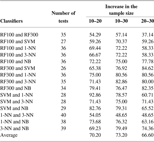
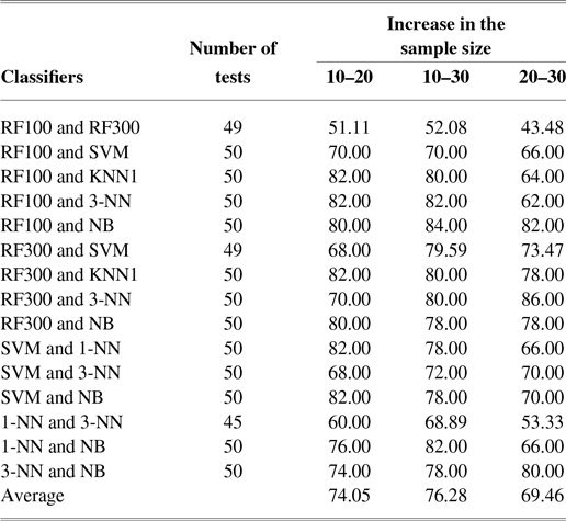
Table 4 shows that, as expected, this sensitivity (p-value reduction with sample size increase) was quite frequent in the analyzed cases. For each pair of classifiers, this table presents the number of tests executed, according to the requirements established in Section 4.1, and the percentage of these tests where the p-value fell as the sample size increased (from 10 to 20, from 10 to 30 and from 20 to 30). This percentage represents the sensitivity in question. For example,
 $92.86\%$
of the 28 comparisons conducted using SVM and 1-NN presented a reduction of the p-value with the increase of the sample size from 10 to 20. It is worth remembering that only the comparisons that satisfied the requirements presented in Section 4.1 were considered in this analysis.
Percentage of applied t-tests in which the p-value fell with the increase in sample size (from 10 to 20, from 10 to 30 and from 20 to 30)

Table 4 shows that, for some pairs of classifiers, the p-value decreased with a frequency higher than for other pairs. However, on average (see the last row of the table), the p-value does tend to decrease as the sample size goes up. This reduction is not a strict rule; there are many exceptions. Probably because, in the larger samples, the new estimates of statistics such as the sample mean and the variance can be different from the estimates of the smaller sample, which can influence the new observed p-values.
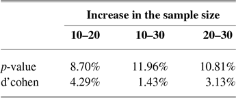
Now, we analyze the percentage of cases where the decrease of the p-value—as a consequence of the sample size increase—changed the conclusion drawn from the hypothesis test, that is, when the result changed from non-significant (p-value
 $\geq$
0.05) to significant (p-value < 0.05). When the sample size increased from 10 to 20, from 10 to 30 and from 20 to 30, the percentages of tests with this conclusion change were
 $8.7\%$
,
 $11.96\%$
and
 $10.81\%$
, respectively. These values are reported in Table 5 and show that a hypothesis test’s sensitivity to sample sizes can affect a substantial number of research results.
Percentages of results where the conclusion changed as the sample size increased, when using the t-test

These results confirm that the sensitivity of the p-value to the sample size is indeed a reason for criticism. Another criticism is that the p-value does not measure the importance (strength) of the result; it only indicates if the result has statistical significance. According to Berben et al. (Reference Berben, Sereika and Engberg2012), the use of the p-value as sole measure can lead researchers to confuse statistical significance with practical or scientific relevance. A statistically significance result does not ensure that the difference is large or relevant in practice, and this should be clear when interpreting the result of the test.
One way to complement the analysis is to use a measure of the effect size, since making decisions based on isolated p-values can lead to misleading conclusions, as will be shown in the next subsection.
4.1.2 Interpreting effect sizes
We now add to the study the effect size measure d’cohen, which is calculated as shown in Equation (15), in Section 2. This measure will be used to evaluate the relevance of the difference between the mean accuracies of the classifiers.
A major reason to measure the effect size along with a test’s p-value is that, unlike the p-value, the effect size is not very sensitive to the sample size. This issue has also been discussed in other areas, for example, in Fern and Monroe (Reference Fern and Monroe1996), Fritz et al. (Reference Fritz, Morris and Richler2012) and Sullivan and Feinn (Reference Sullivan and Feinn2012).
While the p-value indicates whether there is evidence that the difference is really observed in the populations, the effect size indicates the relevance of this difference in the population. Thus, the p-value and the effect size evaluate different aspects of a result and, as noted earlier, may point to opposite paths: p-value indicating statistical significance and effect size small or insignificant, or p-value not indicating statistical significance and effect size medium or large. These are the so-called special cases, discussed in Section 3.
Two analyses are conducted next: the first one studies the behavior of the effect size with an increase in sample size, to compare it with the behavior of the p-value for the same increase, and the second one studies the frequency of the so-called special cases (where there is a disagreement between the p-value and the effect size) in the observed results.
In the first analysis, Table 5 shows the percentages of tests where a change in the p-value and effect size results led to a change in the conclusion, as the sample size increased. The first row shows the percentages of tests whose results were not significant but, with the increase of the sample size, became significant. The second row shows the percentages of tests that indicated small or insignificant effect size and whose results changed to medium or large as the sample size increased, from 10 to 20, from 10 to 30 and from 20 to 30. For example, with the increase of the sample size from 10 to 20, 8.70% of the non-significant cases became significant and 4.29% of the cases with small or insignificant effect size became cases with medium or large effect size.
As shown in Table 5, the percentage of tests where the effect size changed from small or insignificant to medium or large was considerably smaller than the percentage of tests where the p-value result changed from non-significant to significant, for the three cases of an increase in sample size. Note that, despite not being directly sensitive to the sample size, the effect size values have increased or decreased with the increases in sample size. This is due to the estimates (mean and variance) for larger samples being different from the ones for smaller samples—and not due to the use of larger sample sizes.
To illustrate the difference between the behavior of the p-value and the effect size when increasing the sample size, a specific case is presented: the previous comparison between the accuracies obtained by the SVM and 1-NN classifiers using the dataset ‘Contraceptive Method Choice’. With sample size 10, the p-value was higher than 0.05 and, with sizes 20 and 30, it was smaller than 0.05. However, the effect size did not change with the increase of the sample size. The effect size was
 $0.59$
,
 $0.72$
and
 $0.60$
for sample sizes 10, 20 and 30, respectively—all of these rated as a medium effect size.
The second and main analysis focuses on the special cases (where there is disagreement between the p-value and the effect size). In this study, cases were found where the difference between the means of the population accuracies is statistically significant, although the effect size of this difference is small. Cases were also found where there is no statistical significance for this difference and the effect size is medium. And, of course, there were also cases where these two measures agree: cases with statistical significance and a medium or large effect size, and cases with no statistical significance and with a small or insignificant effect size.
Still regarding the comparison of SVM and 1-NN using the dataset ‘Contraceptive Method Choice’, for the sample sizes 20 and 30, the conclusions for the p-value and effect size agree: the difference between the population accuracy means is statistically significant and the effect size is medium. For the sample size 10, the difference between the population accuracy means is not significant, but the effect size is medium—characterizing a special case.
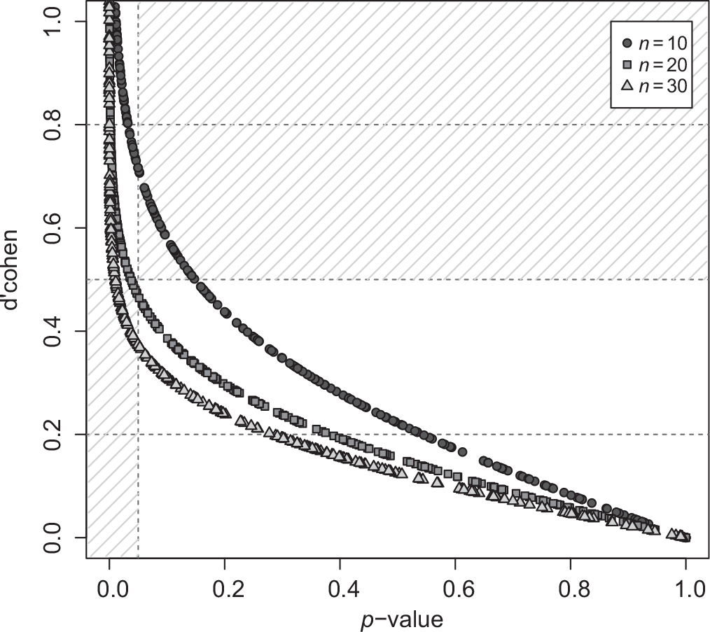
Figure 2 shows the behavior of the p-value and the effect size for each sample size. The shadowed areas set the boundaries for the special cases and each point in the curves represents a performed test. All of the 1509 test runs are depicted. Each curve represents a different sample size. For example, each point in the curve made of circles represents a test conducted with sample size 10 and the points in the shadowed area represent cases with no statistical significance and medium effect size.
Representation of the p-values for t-tests applied to samples sized 10, 20 and 30, and the respective values of effect size—the cases in the shadowed areas represent the special cases

As shown in Figure 2, in most cases the p-value and the effect size agree: the p-value is significant (p-value < 0.05) and the effect size is medium or large (d’cohen
 $\geq$
0.5), or the p-value is not significant (p-value
 $\geq$
0.05) and the effect size is small or insignificant (d’cohen < 0.5). However, for the three sample sizes, special cases were also found where these measures do not agree. The percentage of special cases, and consequently the percentage of agreement cases, is shown in Table 6 (discussed later).
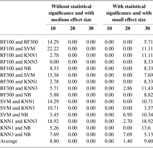
Percentage of datasets with no statistical significance in the t-test and with a medium effect size, and percentage of datasets with statistical significance and small effect size, for each pair of classifiers, per sample size

These special cases are in the shadowed area of Figure 2. Note that the tests with sample size 10 had a specific type of disagreement, whilst tests with sizes 20 and 30 had another kind of disagreement. With sample size 10, in some cases the t-test’s p-value did not allow us to conclude that the classifiers have different accuracies, but the d’cohen value suggested that the effect size is medium. With sample sizes 20 and 30, in some cases the t-test’s result gave us evidence to reject the null hypothesis (p-value < 0.05), concluding that the classifiers have different accuracies, but the effect size was small.
Table 6 shows, for each pair of classifiers and each sample size, the percentage of datasets (out of the 50 datasets used in our experiments) where each of the following types of special cases occurred: (i) cases with no statistical significance in the t-test and a medium effect size, and (ii) cases with statistical significance in the t-test and a small effect size.
The results clearly show that cases with no statistical significance (p-value
 $\geq$
0.05) and a medium effect size (indicating a potentially relevant difference in accuracies) were found only when the cross-validation used 10 folds. The percentage of datasets with this type of special case was over 10% for 6 of the 15 classifier pairs, and it was on average (over all classifier pairs)
 $8.8\%$
.
In Table 6, we only find cases with a statistical significance in the t-test and a small effect size for tests with sample sizes 20 and 30. Besides, this type of special case was observed in all pairs of classifiers for sample size 30. As for the sample size 20, this type of special case was found for only four pairs of classifiers and with low frequencies. On average, the percentages of datasets where the special case of statistical significance and a small effect size was found, for sample sizes 20 and 30, were
 $1.4\%$
and
 $9.6\%$
, respectively.
It should be noted that the special cases do not necessarily indicate an error, since the p-value and the effect size measure different properties. However, this disagreement is evidence that the data deserve more attention. Had we used only the p-value, this might have led to a wrong conclusion. The power of the test is another measure that should be calculated in any study that relies on statistical significance testing, to evaluate the adequacy of the test in the context it is being applied.
4.1.3 Evaluating the power of the test
Now, we add to the analysis the power of the Student’s t-test. As shown in Equation (12) (Section 2), the power of the test is the probability of rejecting the null hypothesis for a given
 $\mu_D$
. In this work, the power of the test is the probability of the test to indicate that classifiers A and B have different accuracies, given the actual difference (estimated by the observed samples difference).
The application of a hypotheses test should always be accompanied by the calculation of the power of the test, to measure its efficiency in the available sample.
Hence, the behavior of the power of the test will be evaluated along with the p-value and the effect size. To that end, we will consider cases where the p-value and the effect size agree, and also the special cases.
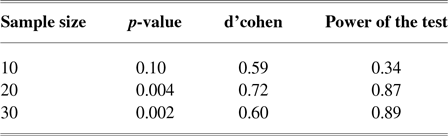
At first, we will verify the power of the t-test for the scenario discussed earlier (comparing SVM’s and 1-NN’s accuracies in the ‘Contraceptive Method Choice’ dataset). As reported in Table 7, the p-values were
 $0.10$
,
 $0.004$
and
 $0.002$
, and the d’cohen values were
 $0.59$
,
 $0.72$
and
 $0.60$
for sample sizes 10, 20 and 30, respectively. For sample size 10, the difference between the classifiers’ accuracies was not statistically significant, but the effect size was medium. The power of the test in this case was
 $0.34$
, a low power (the recommended value is over
 $0.8$
), suggesting that the test was not applied in a ideal scenario, that is, the sample is small. For sample sizes 20 and 30, the t-test indicated a significant difference between the classifiers’ accuracies, whilst the d’cohen value suggests that this difference has a medium effect size. To reinforce these conclusions, the power of the test was
 $0.87$
and
 $0.89$
for sample sizes 20 and 30, respectively, that is, the test has a high probability of rejecting the null hypothesis when it is actually false.
Power of the t-test, p-value and effect size, when comparing SVM’s and 1-NN’s accuracies in the ‘Contraceptive Method Choice’ dataset

Next, in order to facilitate the analysis, we study how the power of the test behaves in each of the following four groups of results:
-
• Group 1: With statistical significance and medium or large effect size
-
• Group 2: Without statistical significance and small or insignificant effect size
-
• Group 3: Without statistical significance and medium or large effect size
-
• Group 4: With statistical significance and small or insignificant effect size
In Groups 1 and 2, the t-test’s p-value and the effect size are in agreement, whilst in Groups 3 and 4, these two measures point to opposite conclusions, that is, they are special cases.
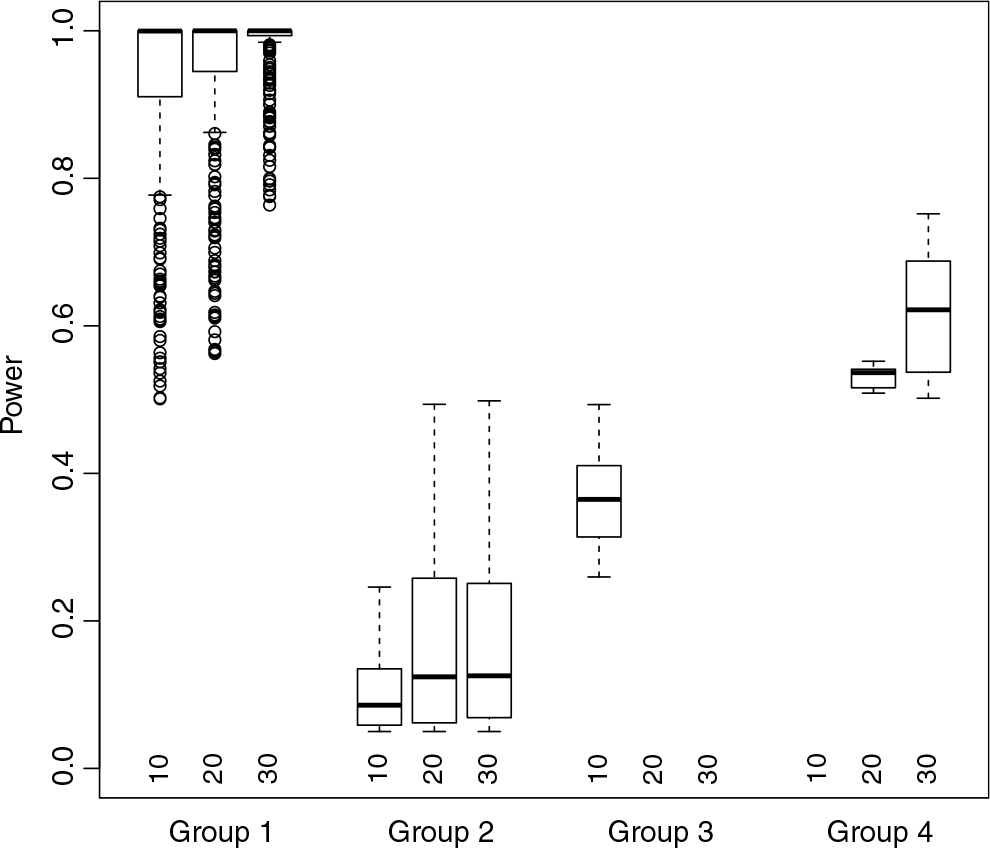
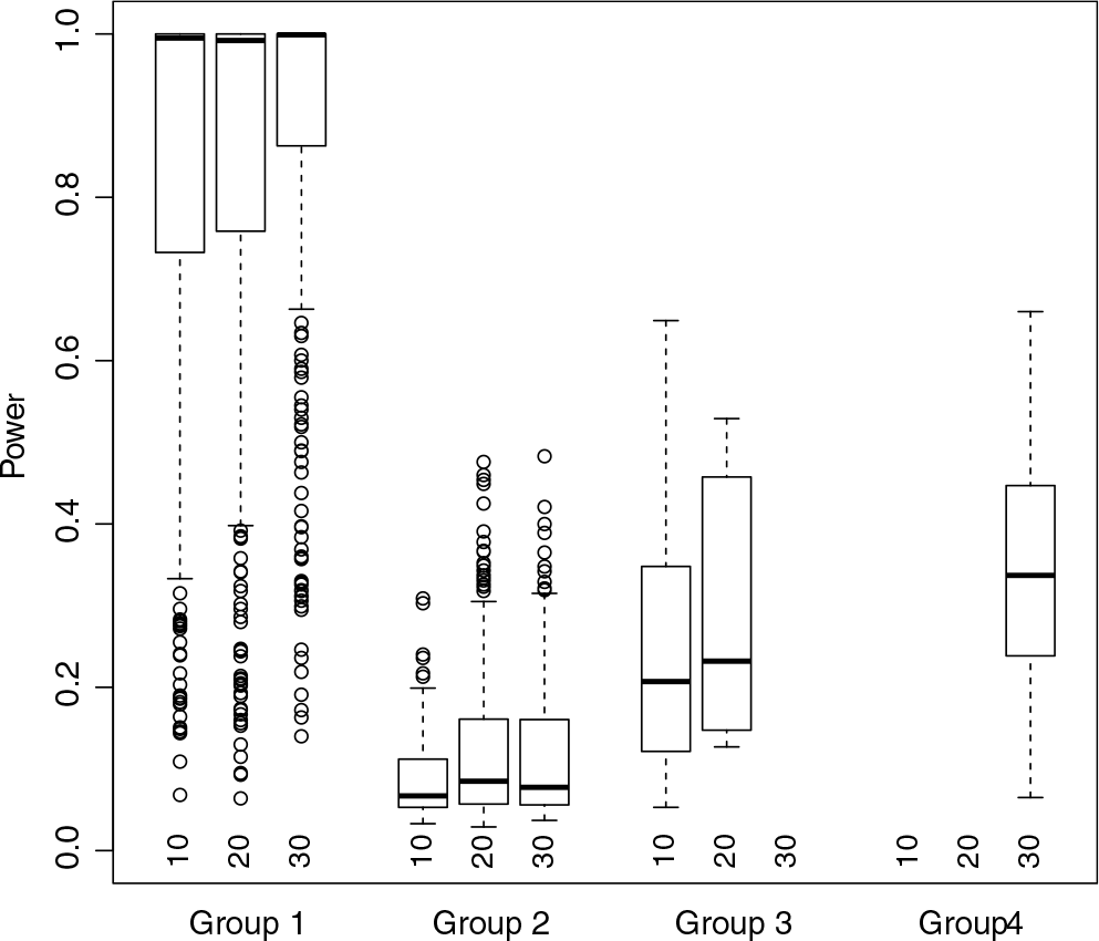
Figure 3 shows the boxplots for the values of the power of the test for these groups, for each sample size (10, 20 and 30). The boxplot is a graphical representation used to evaluate the empirical distribution of a set of values, where the centre box is made by the first, second (median) and third quartiles,
 $Q_1$
,
 $Q_2$
and
 $Q_3$
, respectively. The lower and upper bars extend, respectively, from the lower quartile until the smallest value not exceeding the lower limit
 $(Q_{1}-1.5(Q_{3}-Q_{1}))$
and from the upper quartile to the highest value not exceeding the upper limit
 $(Q_{3}+1.5(Q_{3}-Q_{1}))$
. The points outside these boundaries are considered outliers, represented by circles.
Boxplots for the power of the t-test, per group and sample size

Figure 3 shows that, in Group 1, with statistical significance and a medium or large effect size, in general the power of the t-test was high, with only a few outliers scoring below 80% for the three sample sizes. In this scenario, the three measures reinforce each other: the t-test’s high power gives credibility to its result (a significant difference between the classifiers’ accuracies), and the effect size indicates that this difference is large or relevant.
In Group 2, opposite results were found. The t-test did not reject the null hypothesis and the effect size is small, agreeing with the test’s result. However, the power of the test is small, indicating a low probability of the test rejecting the null hypothesis when it is really false.
Figure 3 also shows that, for the Group 3, containing only cases with sample size 10, the power of the test was low, suggesting that the sample size is too small for applying the t-test. Regarding Group 4, containing only cases with sample sizes 20 and 30, the power of the test (between 50% and 60% for sample size 20 and between 50% and 70% for size 30, approximately) indicates that the probability of the test rejecting the null hypothesis when it is false is only around 60% for these cases. As the effect size is low, we can make an analogy with the example of the aspirin study given in the Introduction: the difference is statistically significant but may not have practical significance.
Note that all the cases with a high power of the test (
 $>0.8$
) belong to Group 1, that is, cases with statistical significance in the t-test and a medium or large effect size, as shown in Figure 3. To better understand this result, recall that, as shown in Subsection 2.2, the parameter
 $\mu_D$
(the difference between population means) is one of the factors that influence the power of the test function, and we used the estimate
 $\mu_d$
(difference between sample means) to calculate this function.
The highest values of sample differences belong to Group 1. For these higher values, it is more likely that the test will obtain a statistical significance and have a medium or higher effect size, as well as a high power of the test. Indeed, these types of results were observed for the three measures. On the other hand, for small sample differences, it is less likely that these three measures could produce these results, although that is not entirely impossible.
In Group 3, even with the small sample differences, the effect size was medium or large. This result can be explained by the small standard deviation for the differences between the sample accuracies. As for Group 4, even with the small sample differences, the t-test showed statistical significance, indicating that there was a difference between the classifiers’ accuracies.
4.2 Analysis with the Wilcoxon test
In this section, we analyze the results for the p-value, effect size and power of the Wilcoxon test, when comparing the same 15 pairs of classifiers in the same 50 datasets as used earlier for the t-test.
As the Wilcoxon test is a non-parametric test, it is not necessary to run a normality test. The only requirement is that the samples with 10, 20 and 30 folds do not have a variance equal to zero.
In the two-sided Wilcoxon test for paired samples, the null hypothesis is that the median of the differences of the classifiers’ accuracies is equal to zero. The alternative hypothesis is that the median of the differences is not zero. These hypotheses are also given in Equation (10), in Section 2.
The following results are organized into three subsections. The first one analyzes how the p-value behaves with the change in sample size. The second one compares the behavior of the p-value and the effect size, whilst the third one also considers the power of the test.
4.2.1 Analysis of the behavior of the p-value
In this subsection, we analyze the impact on the p-values obtained with the Wilcoxon test for different sample sizes when evaluating classifiers, as done in Subsection 4.1.1 for the p-values obtained with the t-test.
The same scenario used in Section 4.1 (to discuss the results for the t-test) will be used here for discussing the results for the Wilcoxon test: the comparison of the accuracies obtained by SVM and 1-NN in the ‘Contraceptive Method Choice’ dataset. We first analyze the sensitivity of the p-value to the sample size. With sample sizes 10, 20 and 30 (cross-validation with 10, 20 and 30 folds) the p-value was
 $0.08$
,
 $0.003$
and
 $0.004$
, respectively. That is, the difference between the classifiers’ accuracies was not significant with sample size 10, but the difference was significant with sample sizes 20 and 30.
Table 8 shows that, as expected, this p-value reduction with sample size increase was quite frequent across the conducted tests. For each pair of classifiers, the table shows the number of tests executed, according to the requirements established in Section 4.2, and the percentage of the conducted tests in which the p-value fell with the increase of the sample size, from 10 to 20, from 10 to 30 and from 20 to 30. For example, in about 82% of the 50 tests executed in the comparison between SVM and 1-NN, the p-value was reduced when the sample size increased from 10 to 20. Opposite from the analysis with the Student’s t-test conducted in Section 4.1.1, in the current analysis, almost all datasets, that is, almost all comparisons, were considered, since the Wilcoxon test is non-parametric and the only requirement is that the samples do not have a variance equal to zero.
Percentage of applied Wilcoxon tests in which the p-value fell with the increase in sample size (from 10 to 20, from 10 to 30 and from 20 to 30)

Table 8 shows that, for some pairs of classifiers, the p-value decreased more often than for other pairs. However, on average (see the last row of the table), the p-value does tend to decrease as the sample size goes up. However, this reduction is not a strict rule; there are many exceptions. As discussed earlier, this is likely because, in larger samples, the estimates of the sample mean and variance tend to be different from the estimates for smaller samples.
As in the earlier t-test analyses, the results reported here show that the p-value obtained with the Wilcoxon test is indeed sensitive to the sample size.
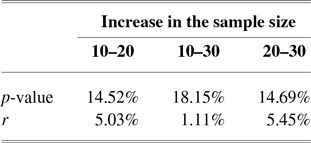
Next, we evaluate in how many cases the reduction of the p-value changed the Wilcoxon test’s conclusion from non-significant to significant. The percentage of cases with such conclusion change, as the sample size increased from 10 to 20, from 10 to 30 and from 20 to 30, was
 $14.52\%$
,
 $18.15\%$
and
 $14.69\%$
, respectively. These values are reported in Table 9. Although they seem low if compared to the observed percentages of p-value reductions, they show that such sensitivity to the sample size can affect a substantial number of research results.
Percentages of results where the conclusion changed as the sample size increased, using Wilcoxon test

4.2.2 Interpreting effect sizes
In this subsection, the measure r for the effect size is added to the study, as defined in Equation (16), in Section 2. The effect size will be calculated for all tests done in order to measure the relevance of the difference between the classifiers’ accuracies, for each dataset. The higher the effect size, the greater the manifestation of the phenomenon (difference) in the population.
Two analyses will be conducted. The first one investigates the behavior of the effect size with an increase in sample size, to compare it with the behavior of the p-value for the same increase. The second one investigates the frequency of the so-called special cases (where there is a disagreement between the p-value and the effect size) in the results for the Wilcoxon test.
The first analysis refers to Table 9, where the first row shows the percentages of results that changed from non-significant to significant as the sample size increased. The second row shows the percentage of results where a small or insignificant effect size (r) changed to a medium or large one as the sample size increased. For example, with the increase of the sample size from 10 to 20, 14.52% of the non-significant cases became significant and 5.03% of the cases with small or insignificant effect size became cases with medium or large effect size.
As shown in Table 9, the percentage of tests where the effect size was upgraded to medium or large was considerably smaller than the percentage of results where the p-value was upgraded to significant, for all three types of sample size increase. Note that, despite not being directly sensitive to the sample size, the effect size has increased or decreased with larger sample sizes, since the estimates of sample mean and variance for larger samples were different from the estimates for smaller samples.
To illustrate this difference between the behaviors of the p-value and the effect size as the sample size increased, we refer again to the comparison between SVM and 1-NN in the ‘Contraceptive Method Choice’ dataset. With sample size 10, the p-value was higher than 0.05, but with sample sizes 20 and 30, it was smaller than 0.05. However, the effect size did not qualitatively change as the sample size increased. The r value was
 $0.39$
,
 $0.45$
and
 $0.3660$
for sample sizes 10, 20 and 30, respectively—all of them a medium effect size.
The second analysis evaluates the frequencies of the special cases, where there is a disagreement between the p-value and the effect size. In the experiments with the Wilcoxon test, similarly to the t-test, cases were found where the difference between the classifiers’ accuracies is statistically significant, although the effect size is small. Cases were also found where the difference is not significant but the effect size is medium. There are also (as expected) cases where these two measures agree: with statistical significance and medium or large effect size, or with no statistical significance and with small or insignificant effect size.
Turning again to our example scenario (comparing SVM and 1-NN in the ‘Contraceptive Method Choice’ dataset), for the sample sizes 20 and 30, the p-value and r measures agree: there is statistical significance and the effect size is medium. For the sample size 10, the difference between the classifiers’ accuracies is not statistically significant, but the effect size is medium, which is considered as a special case.
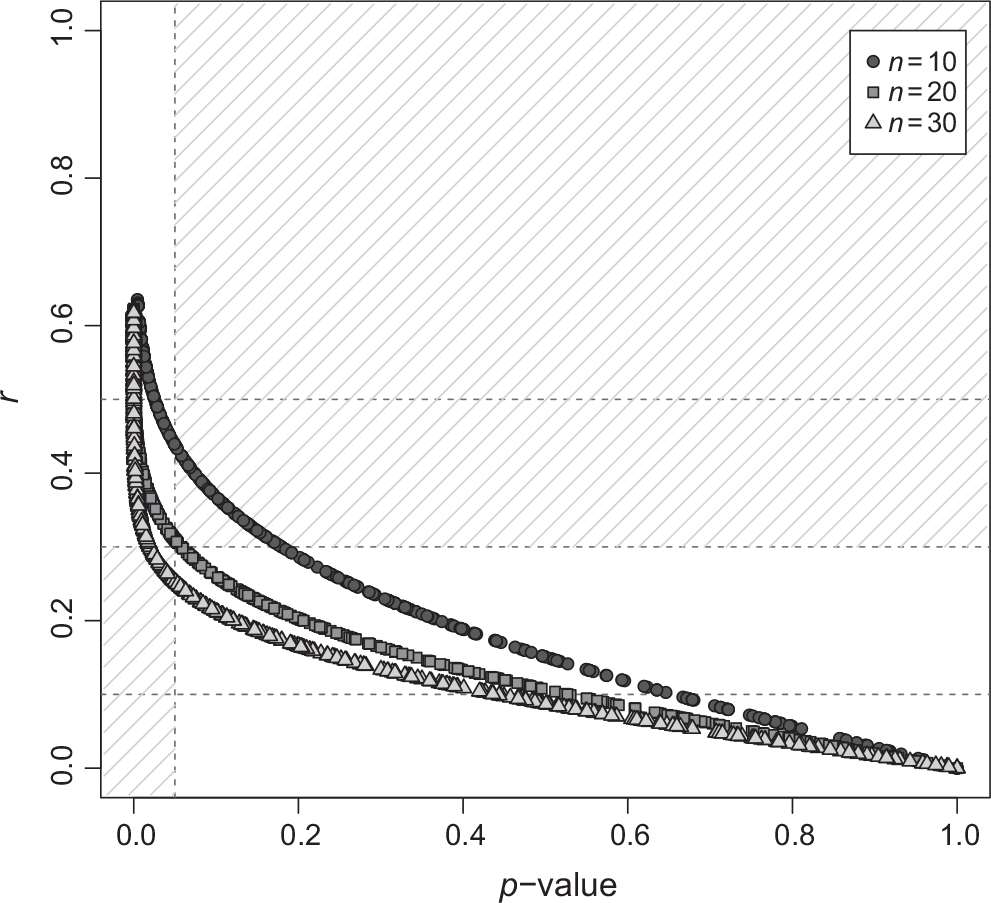
Figure 4 shows the behavior of the p-value and effect size for each sample size. The shadowed areas represent special cases, and each point represents a test result. Each curve refers to a different sample size. For example, each point in the curve made of circles represents a test conducted with sample size 10 and the points in the shadowed area represent cases with no statistical significance and medium effect size.
Representation of the p-values for Wilcoxon tests applied to samples sized 10, 20 and 30, and the respective values of effect size—the cases in the shadowed areas represent the special cases

Note that, for the three sample sizes, in most cases the p-value and the effect size agree. These are cases where: the p-value is statistically significant (p-value < 0.05) and the r measure indicates a medium or larger effect size (
 $r \geq 0.3$
), or the p-value is not significant (p-value
 $\geq$
0.05) and the r measure indicates a small or insignificant effect size (
 $r<0.3$
). However, for the three sample sizes, special cases were also found, where these measures do not agree. These special cases are in the shadowed area of Figure 4. For sample sizes 10 and 20, in some cases the Wilcoxon test’s p-value was not significant, although the r measure for such cases indicated a medium effect size. For sample size 30, some cases were found where the test’s result gave evidence to reject the null hypothesis (p-value < 0.05), although the effect size was small.
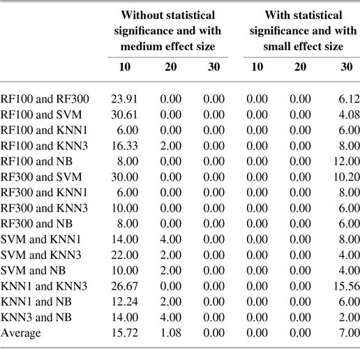
Table 10 shows, for each pair of classifiers and each sample size, the percentages of Wilcoxon test results for each of two types of special cases: (a) with no statistical significance and a medium effect size and (b) with statistical significance and a small effect size. Note that cases without statistical significance and medium effect size were found only for sample sizes 10 and 20. On average over the 15 pairs of classifiers, this type of special case was found in
 $15.72\%$
and
 $1.08\%$
of the results for sample sizes 10 and 20, respectively. For sample size 10, the percentage was over 20% for 5 pairs of classifiers.
Percentage of datasets with no statistical significance in the Wilcoxon test and with a medium effect size, and percentage of datasets with statistical significance and small effect size, for each pair of classifiers, per sample size

Table 10 also shows that cases with a statistically significant p-value and small effect size were found only for samples with size 30. With this sample size, this type of special case was observed for all pairs of classifiers and observed on average for
 $7.0\%$
of the Wilcoxon test results.
It should be noted that, similarly to the t-test results, the sample size 20 led to the smallest percentage of special cases for the Wilcoxon test results.
4.2.3 Evaluating the power of the test
Now, we evaluate the power of the Wilcoxon test, which is calculated based on sample simulation and considering that the actual value of the difference between the classifiers’ accuracies is equal to the observed difference.
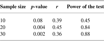
First, we will analyze the power of the test for our example scenario of comparing SVM and 1-NN in the ‘Contraceptive Method Choice’ dataset. As reported in Table 11, the p-value was at
 $0.08$
,
 $0.004$
and
 $0.004$
, and the r effect size was of
 $0.39$
,
 $0.45$
and
 $0.36$
, for sample sizes 10, 20 and 30, respectively. For sample size 10, the difference between the classifiers’ accuracies was not significant, although it had a medium effect size. The power of the test was
 $0.45$
, that is, a low power (the recommended value should be over
 $0.8$
), suggesting that the test was not applied in the ideal scenario. That is, the sample is too small. For sample sizes 20 and 30, the Wilcoxon test’s p-value is statistically significant, whilst the r measure indicated a medium effect size. To reinforce these conclusions, the power of the test was high for both sample size 20 (power
 $0.84$
) and size 30 (
 $0.88$
). This indicates that the test has a high probability of rejecting the null hypothesis when it is actually false.
Power of the Wilcoxon test, p-value and effect size, when comparing SVM’s and 1-NN’s accuracies in the ‘Contraceptive Method Choice’ dataset

The following analyses use the same four groups of results defined in Subsection 4.1.3. Recall that Groups 1 and 2 have agreeing results between the Wilcoxon’s test p-value and the effect size measure r, whilst Groups 3 and 4 are special cases. Figure 5 shows, for each group, the boxplots for values of the power of the Wilcoxon test, for each sample size (10, 20 and 30).
Boxplots for the power of the Wilcoxon test, per group and sample size

Figure 5 shows that in Group 1, with statistical significance and medium or large effect size, in most cases the test had a high power. In this scenario, the three measures reinforce each other: the high power of the test gives credibility to the test’s result, indicating a statistically significant difference between the classifiers’ accuracies, and the effect size indicates that the magnitude of this difference is relevant. However, for this same group, we observe some cases with a low power, with a higher frequency for sample size 10 than for size 30. This is expected, since the power of the test tends to increase as the sample size increases. In this scenario, although the p-value and the effect size agree, a low power indicates that the Wilcoxon test is not reliable.
Group 2 presents an opposite situation. The Wilcoxon test did not reject the null hypothesis and the effect size is small, agreeing with the test’s result. However, the power of the test is low, indicating a low probability of the test rejecting the null hypothesis when it is false.
For Group 3, where the test did not reveal statistical significance but the effect size was medium or large, the power of the test was low. This suggests that the test is unreliable since it has a low probability of rejecting the null hypothesis when the real difference between the classifiers’ accuracy is equal to the sample difference. In these cases, a large effect size and low power of the test point to the fact that the sample size was too small, failing to provide evidence to reject the null hypothesis.
The power of the test was also low in Group 4, where the Wilcoxon test revealed a statistically significant difference between the classifiers’ accuracies, but the effect size was small or insignificant. In such cases, the result of the test is questionable, since it had a low power and small effect size.
As previously observed in the analysis of the Student t-test, the results for the Wilcoxon test also show that all the cases with a high power (
 ${>}0.8$
) belong to Group 1, as seen in Figure 5. That is, the cases with a high power had statistical significance and a medium or large effect size.
It should be pointed out that the largest differences in the sample accuracies belong to Group 1. As expected, for the cases with large observed differences, the test had statistical significance, the effect size was medium or higher and the power of the test was high. However, it is not only in cases with large sample differences that these results are observed. In Group 3, for example, even with the small sample differences, the effect size was medium or large. As for Group 4, even with small sample differences, the Wilcoxon test revealed statistical significance, indicating a difference between the classifiers’ accuracies.
Group 4 has a sample standard deviation slightly larger than the one for Group 3. Despite this and both groups having too small medians and similar distributions, the Wilcoxon test found evidence to reject the null hypothesis in Group 4, but was not able to reject it in Group 3. The difference in these results may be explained by the sample sizes. Although the standard deviation is slightly higher in Group 4, the sample size is also higher in Group 3, which led to these results.
5 Discussion and conclusions
Classifier evaluation based on statistical significance analysis is very important in machine learning and data mining areas, in order to check whether a classifier really outperforms another. Such statistical significance is typically verified by checking whether some hypothesis test’s result allows us to reject the null hypothesis that two (or more) classifiers have the same predictive accuracy.
Despite the usefulness of hypothesis tests, they can lead to wrong conclusions if not properly used. The isolated analysis of a p-value is a problem discussed in several areas (Kline Reference Kline2004; Nakagawa & Cuthill Reference Nakagawa and Cuthill2007; Sullivan & Feinn, Reference Sullivan and Feinn2012; Tomczak & Tomczak Reference Tomczak and Tomczak2014), since it is very common to blindly search for a p-value < 0.05, ignoring the effect size. In a survey of all articles published in the Machine Learning journal in 2017 (ML Journal Reference Journal2017), nine articles used some hypothesis test to compare classifiers, and in all those articles the conclusion about statistical significance was drawn based only on p-values.
Given the limitations of an isolated analysis of p-values as discussed in this work, it is possible that a number of studies are valuing unimportant results, or not recognizing potentially relevant results. In order to investigate these problems, as well as their solutions based on measuring the effect size and the power of the hypothesis test used, we performed experiments with 50 real-world datasets.
Our results reinforce the occurrence of the above problems and support the approach of performing an analysis using not only p-values but also the effect size. In experiments with the Student’s t-test and the Wilcoxon test, applied to datasets with different sample sizes (
 $n = 10, 20, 30$
)—implementing cross-validation with 10, 20 and 30 folds—the p-value was sensitive to the sample size, whilst the effect size did not exhibit a tendency to be sensitive to the sample size.
In addition, it is worth emphasizing that the term statistical significance does not mean significance in practice (for decision-making in the real-world). Actually, we have observed cases where the p-value indicates a statistically significant difference between two classifiers’ accuracies, but the effect size for that difference is small. We have also observed the opposite results, without a statistically significant difference, but with a medium effect size—potentially relevant in practice. Such cases, where the p-value and the effect size suggest different conclusions, were called special cases in this work.
The special cases should not be considered errors, and they deserve special attention, since they are cases where the usual approach of considering only the p-value would lead to ignore the important information about effect size, which could lead to a different conclusion. Note that, in our experiments, the relative frequency of special cases was substantial in some scenarios. To be precise, in the experiments with the t-test applied to the sample sizes of 10, 20 and 30, the special cases represented
 $8.8\%$
,
 $1.4\%$
and
 $9.6\%$
of all test results, respectively. In the experiments with the Wilcoxon test, the relative frequencies of special cases were
 $15.7\%$
,
 $1.1\%$
and
 $7.0\%$
, respectively.
In addition to highlighting the importance of the effect size, these results show that the special cases occurred less frequently in samples of size 20. Hence, when performing a single run of cross-validation, in order to increase the chances of obtaining an agreement between the statistical (p-value) and practical (effect size) measures of significance, researchers and practitioners could choose to use 20 folds, instead of 30 folds or the more commonly used 10 folds. Note, however, that this choice does not deny the importance of calculating the effect size, which remains important in any study aiming at decision-making in practice.
Another problem of considering only p-values is to ignore the power of the test, which is the probability of rejecting the null hypothesis (concluding that the classifiers have different accuracies) given the actual value of that difference. Hence, when the test has a low power, the test’s result is not reliable.
The results reported in this work show the importance of calculating the power of the test. Note that, in the context of comparing classifiers, the sample size for the hypothesis test is typically small. Hence, in many cases the test can have a low power, as observed in our experiments. This shows that ignoring the power of the test can lead to unreliable results in many cases.
The calculation of the power of the test also provides valuable information for analyzing the special cases. Researchers should not abandon the study just because there was no statistical significance when using a test with low power. The medium or large effect size would justify further investigation.
Note that it is also possible to have cases where the test has a high power and the result is statistically significant, but the effect size is small. In such cases, one can conclude that the statistical significance was likely due mainly to the use of a large sample size, since there were enough data to reject the null hypothesis despite the small difference in the classifiers’ accuracies. It is worth recalling the real-world case of the wrong conclusion based on the statistical significance of results for aspirin (Sullivan & Feinn, Reference Sullivan and Feinn2012), as briefly discussed in the Introduction. Such cases reinforce the principle that statistical significance tests should not be responsible for validating or discarding the results of scientific research (Wasserstein & Lazer, Reference Wasserstein and Lazar2016). The result of a statistical significance test indicates a path for the analysis, but researchers should also consider other measures, like the effect size and the power of the test, in order to avoid drawing wrong conclusions.
To summarize the main findings of the article, Table 12 shows a 2 × 2 matrix, considering the four possible types of results involving combinations of two types of effect size (small vs. medium or large) and two types of statistical significance result (p-value < 0.05 vs. p-value
 $\geq$
0.05) for the difference between the mean accuracies of two classifiers. The special cases discussed in this paper correspond to the two cells in the main diagonal of the matrix (i.e., top-left and bottom-right quadrants).
A 2 × 2 matrix summarizing the main findings of the paper

As future work, several research directions can be mentioned: (i) to extend the current study to include other hypothesis tests, for example, Friedman and ANOVA, in order to compare the accuracies of more than two classifiers in a set of datasets; (ii) to use other approaches to get samples of classifier accuracies, for example, multiple cross-validation runs; (iii) to perform a theoretical study to try to explain why in our cross-validation experiments the sample size of 20 folds led to a substantially smaller number of special cases, which would reinforce the recommendation of using this sample size when an agreement between the statistical and practical significances is an important aspect of the data analysis and (iv) to compare the use of p-values, properly complemented with the measures of effect size and power of the test, with the Bayesian approach, proposed by Benavoli et al. (Reference Benavoli, Corani, Demšar and Zaffalon2017) as an appropriate alternative to evaluate the statistical significance of classifiers’ results.
In summary, considering the empirical evidence and the arguments discussed along this article, it is recommended that the analyses of statistical significance in the areas of machine learning and data mining be extended to consider a measure of effect size and the power of the hypothesis test, in order to draw more statistically principled conclusions.