1. Introduction
The falling or rising of Newtonian and non-Newtonian drops in another liquid has a wide range of industrial applications. During the flocculation process, the sedimentation rate and, therefore, the drag coefficient depend on various parameters such as droplet size and the rheological properties of the viscoelastic material. Furthermore, such fundamental studies play crucial roles in processes such as coating (Deng et al. Reference Deng, Schellenberger, Papadopoulos, Vollmer and Butt2013), spray painting (Herczyński et al. Reference Herczyński, Cernuschi and Mahadevan2011), spray cooling (Grissom & Wierum Reference Grissom and Wierum1981), blending molten polymers (Graebling, Muller & Palierne Reference Graebling, Muller and Palierne1993; Lacroix, Aressy & Carreau Reference Lacroix, Aressy and Carreau1997), ink-jet printers (Martin, Hoath & Hutchings Reference Martin, Hoath and Hutchings2008; Saunders, Gough & Derby Reference Saunders, Gough and Derby2008), as well as the use of immiscible drops in direct-contact heat exchangers (Sideman & Taitel Reference Sideman and Taitel1964; Sideman, Hirsch & Gat Reference Sideman, Hirsch and Gat1965) and nearly miscible drops in liquid – liquid extraction processes (Handlos & Baron Reference Handlos and Baron1957). Viscoelastic materials are used in a wide range of technological applications, spanning biotechnology, mechanical, civil and chemical engineering, as well as food and cosmetic production, and in the development of sophisticated injectable and transdermal drugs. To achieve an appropriate design in such processes, a comprehensive understanding of the drop’s size, shape, deformation and terminal velocity during motion is essential.
Over recent decades, numerous analytical, numerical and experimental studies have investigated the behaviour of drops and bubbles rising or falling through Newtonian and non-Newtonian fluids. In Newtonian creeping flow, the foundational works of Hadamard (Reference Hadamard1911) and Rybczyński (Reference Rybczyński1911) analytically demonstrated that in the absence of inertial forces, the shape of a drop remains spherical. This is due to the linearity of the governing equations, which yields uniform stress distributions and allows the interfacial tension to maintain a spherical interface. Taylor & Acrivos (Reference Taylor and Acrivos1964) extended this framework by including weak inertia using perturbation theory, revealing that at higher Reynolds numbers, drops assume an oblate shape due to the non-uniformity of normal stresses across the interface. The interfacial tension’s inability to resist the stress imbalance leads to interface deformation.
Beyond Newtonian regimes, Smolianski et al. (Reference Smolianski, Haario and Luukka2003) and Clift, Grace & Weber (Reference Clift, Grace and Weber2005) reported significant shape changes in bubbles and drops in Newtonian fluids depending on surface tension, inertial and gravitational forces. For non-Newtonian systems, Gürkan (Reference Gürkan1989) analysed power-law drops in Newtonian media, while Marrucci, Apuzzo & Astarita (Reference Marrucci, Apuzzo and Astarita1970) focused on their terminal velocity under creeping conditions. Sostarecz & Belmonte (Reference Sostarecz and Belmonte2003) experimentally demonstrated that creeping viscoelastic drops become oblate and eventually form a rear dimple as the drop volume increases. Davoodi & Norouzi (Reference Davoodi and Norouzi2016), Vamerzani, Norouzi & Firoozabadi (Reference Vamerzani, Norouzi and Firoozabadi2016) and Mukherjee & Sarkar (Reference Mukherjee and Sarkar2011) further explored the dynamics of viscoelastic drops using analytical and numerical approaches, demonstrating that increased elasticity intensifies flow velocities inside and outside the drop, and reduces its terminal speed. In addition, for viscoelasticity located inside the drop, Wu, Haj-Hariri & Borhan (Reference Wu, Haj-Hariri and Borhan2012) performed a stability analysis of a translating viscoelastic drop in a Newtonian ambient (FENE–CR in the drop phase), delineating how internal elasticity affects the stability of initially oblate versus prolate shapes at low Reynolds number.
Bubble dynamics has also been widely investigated in relation to the velocity jump phenomenon, where a sudden increase in rise velocity is observed beyond a critical bubble size. Funfschilling & Li (Reference Funfschilling and Li2006) tested bubble motion in glycerol, carboxymethyl cellulose and polyacrylamide (PAAm) solutions, finding that in viscoelastic fluids, the velocity increases with a non-trivial dependence on bubble volume. Herrera-Velarde et al. (Reference Herrera-Velarde, Zenit, Chehata and Mena2003) employed particle image velocimetry techniques to visualise wake structures around rising bubbles in PAAm solutions, identifying negative wake formations and vortex asymmetries associated with the velocity jump. Acharya, Mashelkar & Ulbrecht (Reference Acharya, Mashelkar and Ulbrecht1977) proposed that polymer molecules behave like surfactants, modifying the surface mobility and leading to velocity discontinuities. Complementing these experiments, Pillapakkam et al. (Reference Pillapakkam, Singh, Blackmore and Aubry2007) conducted direct numerical simulations of rising bubbles in viscoelastic fluids and characterised the transient approach to steady regimes across parameter ranges. The onset of sharp geometric features has been addressed via linear stability analyses; You et al. (Reference You, Borhan and Haj-Hariri2009a ) examined the stability of cusped bubble shapes in viscoelastic flows and identified conditions for their persistence. More recently, Moschopoulos et al. (Reference Moschopoulos, Spyridakis, Dimakopoulos and Tsamopoulos2024) unravelled asymmetric bubble states in viscoelastic fluids, mapping parameter regimes where symmetry breaking occurs.
Pilz & Brenn (Reference Pilz and Brenn2007) examined bubble motion in dilute polymer solutions and reported that velocity jumps were suppressed at low concentrations. Liu, Liao & Joseph (Reference Liu, Liao and Joseph1995) highlighted cusp formation at the trailing edge of bubbles in elastic fluids, linking it to capillary number thresholds but showing that cusp presence alone is insufficient for a velocity jump. Soto et al. (Reference Soto, Goujon, Zenit and Manero2006) used hydrophobically modified akali soluble emulsion polymer solutions and correlated the rise velocity jump to normal stress contributions via the elastic number
 $\varPi$
. They concluded that above a critical value,
 $\varPi _{{cr}} \approx 0.25$
, a velocity jump is initiated.
Niethammer et al. (Reference Niethammer, Brenn, Marschall and Bothe2019) and Bothe et al. (Reference Bothe, Niethammer, Pilz and Brenn2022) performed direct numerical simulations of rising bubbles in viscoelastic media, capturing velocity jumps and investigating the underlying molecular mechanisms. They demonstrated that the spatial location of elastic energy release, either near the bubble’s top or bottom, has an impact on whether the bubble accelerates or decelerates. These computations also provide mechanistic context for experimental observations by linking localised elastic-stress relaxation to abrupt changes in bubble kinematics.
Beyond bubbles, other studies have focused on drops moving in a viscoelastic external medium. Wagner & Slattery (Reference Wagner and Slattery1971) examined the settling of viscoelastic drops in viscoelastic environments using third-order fluid models and concluded that strong elastic forces may lead to prolate drop shapes. Similarly, Mohan, Nagarajan & Venkateswarlu (Reference Mohan, Nagarajan and Venkateswarlu1972), Lavrenteva, Holenberg & Nir (Reference Lavrenteva, Holenberg and Nir2009) and Wanchoo, Sharma & Gupta (Reference Wanchoo, Sharma and Gupta2003) investigated shape evolution under elastic environments, demonstrating that drops can deform differently depending on their internal and external fluid properties. On the numerical side, You et al. (Reference You, Haj-Hariri and Borhan2009b ) quantified how geometric confinement modifies the velocity and morphology of a Newtonian/viscoelastic two-phase drop system. To enable such simulations, You, Borhan & Haj-Hariri (Reference You, Borhan and Haj-Hariri2008) developed a finite-volume formulation for viscoelastic two-phase flows capable of capturing interfacial motion and stress evolution. Most recently, Esposito, Dimakopoulos & Tsamopoulos (Reference Esposito, Dimakopoulos and Tsamopoulos2023) investigated buoyancy-driven motion of a viscous (Newtonian) drop in viscoelastic materials, validating computations against experiments and mapping terminal states and tail-breakup behaviour.
Despite these advances, existing studies have primarily focused on bubble motion, often overlooking the complex behaviour of rising drops, particularly in scenarios involving low Reynolds numbers, nonlinear viscoelasticity and sharp interfacial deformations. Many previous works rely on creeping flow assumptions, neglect convective effects or apply linear viscoelastic models that fail to capture nonlinear stress interactions.
The present study investigates the dynamics of Newtonian drops rising in viscoelastic fluids – a domain that, despite its practical relevance, remains far less explored than the extensively studied case of gas bubbles. While many studies have documented velocity jumps and wake instabilities for bubbles in viscoelastic media, this work is the first systematic investigation of the phenomenon in Newtonian droplets. This distinction is crucial because the presence of a viscous interior alters the interfacial stress balance and internal flow, introducing additional complexity compared with bubbles. Moreover, existing studies on drop dynamics have typically focused on gradual deformation, drag modification or elongation, but have not reported sharp transitions in rise velocity for Newtonian drops in the absence of interfacial viscoelasticity or surfactants. This lack of evidence has left open the question of whether elasticity in the surrounding medium alone can induce abrupt transitions in drop dynamics. To address this critical gap, we present a combined analytical and experimental investigation. On the theoretical side, a full set of governing equations is solved using a triple perturbation approach, with Reynolds, Deborah and capillary numbers serving as expansion parameters. Unlike earlier analytical models that neglect nonlinear inertia, our framework retains the convective terms, allowing the capture of essential flow features even at finite Reynolds numbers. The Giesekus constitutive model is employed for the viscoelastic medium, providing a realistic representation of polymeric fluids with shear thinning and elastic effects (Soto et al. Reference Soto, Goujon, Zenit and Manero2006; Bothe et al. Reference Bothe, Niethammer, Pilz and Brenn2022). The analytical solution yields closed-form expressions for drop deformation and terminal velocity, establishing a mechanistic link between elasticity-induced normal stresses and flow asymmetry.
One of the main conceptual contributions of this work lies in the theoretical demonstration that elastic normal stress differences in the surrounding fluid can generate asymmetric stress fields around a Newtonian drop, even in the absence of interfacial viscoelasticity. Complementing the analytical work, the experimental component employs high-resolution visualisation techniques to observe drop behaviour under carefully controlled rheological conditions. PAAm solutions of varying concentrations are used as the continuous phase, allowing independent control over elasticity and shear viscosity. The internal (drop) phase remains Newtonian, with systematic variation of the viscosity ratio between the two phases. The set-up is designed to isolate the effects of elasticity and viscosity ratio from other confounding factors such as inertial or surfactant-driven phenomena.
The central novelty of this study lies in its identification and characterisation of a velocity-jump phenomenon in Newtonian drops. This work establishes that abrupt transitions in drop motion are not limited to bubbles or to systems with interfacial elasticity, but can also occur when purely Newtonian drops interact with appropriately structured viscoelastic environments. By unifying a predictive analytical framework with rigorous experimental validation, the study offers a new perspective on how external rheology alone can induce sharp transitions in drop dynamics. This work extends the current understanding of multiphase flow in non-Newtonian fluids by highlighting a novel mechanism, external elastic destabilisation, which drives discontinuities in the motion of Newtonian drops. The findings provide a foundation for future control strategies in applications such as emulsion transport, biomedical devices and industrial fluid systems.
2. Mathematical approach
2.1. Governing and constitutive equations
The governing equations are presented as follows:
 \begin{equation} \boldsymbol{\nabla }\boldsymbol{\cdot }\tilde {\boldsymbol{v}}_{\!j} = 0, \end{equation}
 \begin{equation} \tilde {\rho }_{\!j} \frac {{\rm D}\tilde {\boldsymbol{v}}_{\!j}}{{\rm D}\tilde {t}} = -\boldsymbol{\nabla }\!\tilde {p}_{\!j} + \tilde {\rho }_{\!j} {\tilde {\boldsymbol{g}}} + \boldsymbol{\nabla }\boldsymbol{\cdot }\tilde {\boldsymbol{\tau }}_{\!j}, \end{equation}
where
 $ j = i, e$
,
 $\tilde {\boldsymbol{v}}$
represents the velocity vector,
 $\tilde {\rho }$
denotes the density,
 $\tilde {p}$
signifies the pressure,
 $\tilde {\boldsymbol{\tau }}$
corresponds to the extra stress tensor and
 $\tilde {\boldsymbol{g}}$
denotes the uniform gravitational acceleration vector, identical in both phases; buoyancy enters solely through the phase densities
 $\tilde {\rho }_{\!j}$
. For definiteness, we take
 $\tilde {\boldsymbol{g}}=-\,\tilde {g}\,\boldsymbol{e}_z$
. The indices
 $i$
and
 $e$
indicate the interior and exterior fluids, respectively, referring to the rising Newtonian drop and the surrounding non-Newtonian fluid. In the present study, the droplet density is lower than that of the host liquid, so droplets rise under buoyancy. The same analysis applies for
 $\rho _{\textit{drop}}\gt \rho _{\textit{host}}$
, in which case, the motion would be downward with the sign of the terminal velocity reversed. All dimensional parameters are consistently marked with a tilde. In the rest of the paper, the effect of gravitational acceleration is implemented in the modified pressure. The geometry of the study is shown in figure 1. The present analytical formulation is based on an axisymmetric representation of the velocity field around the vertical axis. While full axisymmetry cannot be strictly guaranteed in the supercritical regime, where elastic effects may lead to localised stress concentration and asymmetric deformation, the axisymmetric approach remains valuable for elucidating the fundamental mechanisms governing the flow. This framework enables a clear interpretation of how viscoelastic normal stresses evolve, intensify and redistribute around the droplet interface as elasticity increases.
Schematic representation of the geometry under investigation.

In this study, the Giesekus model is employed as the constitutive framework for analysing viscoelastic media. Recognised as a nonlinear constitutive equation, the Giesekus model has demonstrated reliability in accurately representing a wide range of viscoelastic flow behaviours. The mathematical formulation of the Giesekus model is given by Bird, Armstrong & Hassager (Reference Bird, Armstrong and Hassager1987):
 \begin{equation} \tilde {\boldsymbol{\tau }}=\tilde {\boldsymbol{\tau }}_p+\tilde {\boldsymbol{\tau }}_s, \end{equation}
 \begin{equation} \tilde {\boldsymbol{\tau }}_p+ \tilde {\lambda } {\overset {\boldsymbol{\nabla }}{\tilde {\boldsymbol{\tau }}_p}} +\frac {\alpha \tilde {\lambda }}{\tilde {\eta }_{p,0}} \left ( \tilde {\boldsymbol{\tau }}_p \boldsymbol{\cdot }\tilde {\boldsymbol{\tau }}_p \right )=2\tilde {\eta }_{p,0}\tilde {\unicode{x1D63F}}, \end{equation}
 \begin{equation} \tilde {\boldsymbol{\tau }}_s=2\tilde {\eta }_{s}\tilde {\unicode{x1D63F}}. \end{equation}
The extra stress is formulated as the sum of the stresses contributed by the Newtonian solvent,
 $\tilde {\boldsymbol{\tau }}_s$
, and the polymeric additive,
 $\tilde {\boldsymbol{\tau }}_p$
. In this context,
 $\tilde {\eta }_s$
denotes the viscosity of the Newtonian solvent, while
 $\tilde {\eta }_{p,0}$
represents the polymeric contribution to the viscosity at zero shear rate. Furthermore,
 $\tilde {\unicode{x1D63F}}=0.5 ( \boldsymbol{\nabla }\boldsymbol{\tilde {v}} +\boldsymbol{\nabla }{\boldsymbol{\tilde {v}}}^{{T}} )$
and
 $\tilde {\lambda }$
correspond to the rate-of-deformation tensor and the relaxation time, respectively. The parameter
 $\alpha$
serves as the model mobility factor, derived from anisotropic Brownian motion and/or anisotropic hydrodynamic drag acting on the constitutive polymer molecules (Bird et al. Reference Bird, Armstrong and Hassager1987). The upper convective derivative,
 $\overset {\boldsymbol{\nabla }}{}$
, is defined as follows:
 \begin{equation} {\overset {\boldsymbol{\nabla }}{\unicode{x1D63D}}}= \left (\frac {\partial }{\partial \tilde {t}}+\tilde {\boldsymbol{v}} {\boldsymbol{\cdot }} \boldsymbol{\nabla }\right )\unicode{x1D63D} -\big(\left (\boldsymbol{\nabla }{\tilde {\boldsymbol{v}}}\right )^T {\boldsymbol{\cdot }} \unicode{x1D63D}+\unicode{x1D63D} \boldsymbol{\cdot }\boldsymbol{\nabla }{\tilde {\boldsymbol{v}}}\big ) ,\end{equation}
where
 $\unicode{x1D63D}$
represents an arbitrary second-order tensor. The following parameters are used to non-dimensionalise the governing equations:
 \begin{equation} \begin{array}{lllll} {\textit{De}}=\dfrac {\tilde {\lambda } \tilde {V}_\infty }{2\tilde {R}}, & \textit{Re}=\dfrac {2\tilde {\rho }_{\textit {e}}\tilde {V}_\infty \tilde {R}}{{\tilde {\eta }_{\textit {e,0}}}}, & {\textit{Ca}}=\dfrac {\tilde {\eta }_{\textit {e}} \tilde {V}_\infty }{\tilde {\sigma }}, & \beta =\dfrac {\tilde {\eta }_{{\textit {p,0}}}}{{\tilde {\eta }_{{e,0}}}}, & {{k}=\dfrac {\tilde {\eta }_i}{\tilde {\eta }_{\textit {e,0}}},}\\ \boldsymbol{\tau }=\dfrac {2\tilde {\boldsymbol{\tau }} \tilde {R}}{{\tilde {\eta }_{\textit {e,0}}} \tilde {V}_0}, & \boldsymbol{v}=\dfrac {\tilde {\boldsymbol{v}}}{\tilde {V}_0}, & \unicode{x1D63F}=\dfrac {2\tilde {\unicode{x1D63F}} \tilde {R}}{\tilde {V}_0}, & p=\dfrac {2\tilde {p} \tilde {R}}{{\tilde {\eta }_{\textit {e,0}}} \tilde {V}_0}, & {\varGamma =\dfrac {\tilde {\rho _i}}{\tilde {\rho }_e}},\\ \end{array} \end{equation}
where
 $\textit{De}$
is the Deborah number,
 $\textit{Re}$
is the Reynolds number and
 $\textit{Ca}$
is the capillary number. The reference velocity
 $\tilde {V}_0$
is defined as
 $\tilde {V}_0=\tilde {V}_\infty /({k}+1)$
, where
 ${k}$
is the viscosity ratio. Here,
 $\tilde {V}_\infty$
denotes the terminal rising velocity of the drop and
 $\varGamma$
is the density ratio. The equivalent radius
 $\tilde {R}$
of the drop is calculated by
 $(3\tilde {{\varOmega }}/4\pi )^{1/3}$
, where
 $\tilde {{\varOmega }}$
is the volume of the rising drop. Additionally,
 $\tilde {\sigma }$
is the interfacial tension at the interface between the two liquids and
 $\beta$
is the retardation parameter for the exterior medium, representing the ratio of the polymeric viscosity
 $\tilde {\eta }_{{p,0}}$
to the total viscosity
 ${\tilde {\eta }_{{e,0}}}=\tilde {\eta }_s+\tilde {\eta }_{\textit {p},0}$
as the shear rate approaches zero.
To eliminate the unknown pressure gradients in the
 $r$
and
 $\theta$
directions, the curl operator is applied to the momentum equations corresponding to these directions. The relationship between the stream function and the velocity components in the spherical coordinate system is established, as detailed by Bird et al. (Reference Bird, Armstrong and Hassager1987), Wanchoo et al. (Reference Wanchoo, Sharma and Gupta2003) and Landau & Lifshitz (Reference Landau and Lifshitz2013):
 \begin{equation} \boldsymbol{v}_{\!j}\left (r,\theta \right )=\left ( \frac {1}{r^2\sin \theta } \frac {\partial \psi _{\!j}}{\partial \theta }{,} -\frac {1}{r\sin \theta } \frac {\partial \psi _{\!j}}{\partial r} \right )\!,\quad j=i,e. \end{equation}
2.2. Boundary conditions
As an initial step in determining the stress and velocity distributions, the droplet is assumed to be spherical. Based on this assumption, it will be demonstrated that the normal force at the interface is not balanced, indicating that the droplet cannot maintain a perfectly spherical form. Consequently, a more accurate prediction of the droplet shape will be derived to correct this initial approximation (Sostarecz & Belmonte Reference Sostarecz and Belmonte2003). Assuming a spherical geometry, the boundary conditions at the interface between the droplet and the surrounding fluid are defined as follows:
-
(i) at the surface of the drop, the radial velocity components are zero.
-
(ii) The dimensional tangential velocity and shear stress are equal.
-
(iii) It is required that the fluid velocities at the droplet centre and in the far-field (i.e. at infinity) remain finite.
-
(iv) The normal stress balance at the interface is given by (Batchelor Reference Batchelor2000)
(2.9) \begin{equation} \boldsymbol{n} \boldsymbol{\cdot }\left ( \boldsymbol{\tau }_e-\frac {{k}}{{k}+1}\boldsymbol{\tau }_i \right ) \boldsymbol{\cdot }\boldsymbol{n} -p_e+p_i=\frac {1}{{\textit{Ca}}}\left ( \frac {1}{R_1}+\frac {1}{R_2}\right )\!. \end{equation}

In (2.9),
 $\boldsymbol{n}$
is the unit vector normal to the droplet surface, and
 $R_1$
and
 $R_2$
are the principle radii of the curvature of the surface of the droplet. In small deformation cases, the following relationship is justified (You et al. Reference You, Borhan and Haj-Hariri2008):
 \begin{equation} \frac {1}{R_{1}}+\frac {1}{R_{2}}=2-2 \zeta -\frac {\rm d}{{\rm d} \mu }\left (\big(1-\mu ^{2}\big ) \frac {{\rm d} \zeta }{{\rm d} \mu }\right )\!, \end{equation}
where
 $\zeta$
is the deformation function and
 $\mu =\cos (\theta )$
. Eventually, the normal stress balance condition in a dimensionless form can be re-written as
 \begin{equation} \boldsymbol{n} \boldsymbol{\cdot }\left (\boldsymbol{\tau }_{e}-\frac {{k}}{{k}+1} \boldsymbol{\tau }_{i}\right ) \boldsymbol{\cdot }\boldsymbol{n}-p_{e}+p_{i}=\frac {1}{{\textit{Ca}}}\left(2-2 \zeta - \frac {\rm d}{{\rm d} \mu }\left (\big (1-\mu ^{2}\big ) \frac {{\rm d} \zeta }{{\rm d} \mu }\right )\right )\!. \end{equation}
This exact interfacial normal–stress balance will be used later to determine the shape of the droplet, where
 $\zeta$
is the deviation of the droplet shape from spherical. The function
 $\zeta$
satisfies
 $\int _{-1}^{1}\zeta \,{\rm d}\mu =0$
and
 $\int _{-1}^{1}\zeta \mu \,{\rm d}\mu =0$
.
2.3. Perturbation method
In this study, a triple perturbation technique is employed to solve the nonlinear governing equations. The Reynolds number, Deborah number and capillary number are selected as the perturbation parameters. Accordingly, the perturbed expressions for the velocity, pressure, deformation rate, extra stress tensor and stream function are formulated as follows:
 \begin{equation} \begin{array}{l} \varLambda _{\!j}=\left ( \varLambda _{\!j} \right )_{0} + \textit{Re}\left (\varLambda _{\!j}\right )_{1}+\textit{ReCa}\left (\varLambda _{\!j}\right )^{(1)}+ \textit{De}\left (\varLambda _{\!j}\right )_{11}+{\textit{DeCa}}\left (\varLambda _{\!j}\right )^{(11)}; \\ \\ \quad \quad \quad \quad \quad \quad \quad \quad \quad \varLambda =\boldsymbol{v}, p, \unicode{x1D63F}, \boldsymbol{\tau }, \psi , \quad j=i, e. \end{array} \end{equation}
Accordingly, the perturbation scheme treats Re, De and Ca as equally small parameters
 $ (\textit{Re} \sim {\textit{De}} \sim {\textit{Ca}} \ll 1 )$
, naturally generating higher-order mixed terms such as
 $\textit{Re} \boldsymbol{\cdot }{\textit{Ca}}$
and
 ${\textit{De}} \boldsymbol{\cdot }{\textit{Ca}}$
(rather than Ca alone) because interfacial deformation arises only through the nonlinear inertial or elastic contributions, consistent with the classical small-parameter expansions of Taylor & Acrivos (Reference Taylor and Acrivos1964) for viscous drops and Sostarecz & Belmonte (Reference Sostarecz and Belmonte2003) for viscoelastic drops, and ensuring that these combined terms correctly represent the coupled inertial–elastic–capillary mechanisms governing weakly nonlinear flow and deformation.
After collecting the terms at the zeroth order, we have
 \begin{equation} E^{4}\left (\psi _{\!j}\right )_{0}=0,\quad j=i, e, \end{equation}
where
 $E^4=E^2 E^2$
and
 $E^2=({\partial ^2}/{\partial r^2})+({\sin }/{r^2})( {\partial }/{\partial \theta }) ( ( {1}/{\sin {\theta }})( {\partial }/{\partial \theta }) )$
. Happel & Brenner (Reference Happel and Brenner1965) showed that the solution to (2.13) has the following form:
 \begin{equation} \begin{array}{ll} \psi _{\!j}(r, \theta )=\sum _{n=1}^{\infty }\left (A_{n} r^{-n}+B_{n} r^{2-n}+C_{n} r^{n+1}+D_{n} r^{n+3}\right ) Q_{n}(\mu ), & j=i,e, \end{array} \end{equation}
where
 $Q_n (\mu )$
is the Gegenbauer polynomial and
 $Q_n (\mu )=\int _{-1}^{\mu } P_n ( s )\,{\rm d}s$
. Here,
 $P_n$
denotes the Legendre polynomial of degree
 $n$
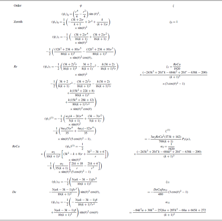
. The results of different terms of the perturbation series for stream and deformation functions are presented in table 1. Here, the solution of the zeroth-order equation is identical with that of Hadamard (Reference Hadamard1911) for Newtonian droplets. The boundary condition for the normal stress balance is formulated as
 $\delta \textit {p}=({1}/{\textit{Ca}} )(( {1}/{R_1})+( {1}/{R_2} ))$
in which
 $\delta \textit {p}$
is the constant ambient pressure jump. For zeroth order, the drop shape is spherical and
 $R_1=R_2=1$
. The deformation function corresponding to the zeroth order is also presented in table 1.
Stream and deformation functions for the different perturbation orders.

The equations of the first order Re stream functions are written as
 \begin{equation} E^4\left (\psi _i\right )_1=0 ,\end{equation}
 \begin{equation} \begin{array}{l} E^{4}\left (\psi _{e}\right )_{1}=-\dfrac {3}{2} \mu \left (1-\mu ^{2}\right )\left (\dfrac { 3 {k} + 2 } { {k} + 1 } \left (\dfrac {1}{r^{2}}-\dfrac {1}{2 \mathrm{r}^{3}} \dfrac {3 {k}+2}{{k}+1}+\dfrac {1}{2 r^{5}} \dfrac {{k}}{{k}+1}\right )\right )\!. \end{array} \end{equation}
By applying the boundary conditions, the solutions for the stream functions corresponding to the order of
 $\textit{Re}$
can be obtained. The boundary condition presented for the normal stress balance can be expressed as
 \begin{equation} \begin{array}{l} \delta p-4\alpha _2\textit{Re} P_2\left (\mu \right )=\dfrac {1}{\textit{Ca}}(-2 \zeta - \left .\dfrac {\rm d}{{\rm d} \mu }\left [\left (1-\mu ^{2}\right ) \dfrac {{\rm d} \zeta }{{\rm d} \mu }\right ]\right )\!, \end{array} \end{equation}
where
 $\delta p={2}/{\textit{Ca}}$
and the deformation function for the order of
 $\textit{Re} (\zeta _1 )$
is obtained in table 1 (
 $\alpha _2$
is defined in the table). The procedure outlined demonstrates that the stream function term, when considered at the order of
 $\textit{Re} {\textit{Ca}}$
, is similar to the zeroth-order approximation
 $ ( E^4 (\psi _{\!j} )^{ (1 )}=0, \; j=i,e )$
. In this study, the stream function is determined by applying the boundary conditions to the newly approximated geometry. To facilitate the analysis, Sostarecz & Belmonte (Reference Sostarecz and Belmonte2003) proposed modifications to the boundary conditions (additional details are provided in Appendix A). By applying the stress balance at the order of the Reynolds and capillary numbers
 $ (\textit{Re} {\textit{Ca}} )$
, we obtain
 \begin{align} \left (-5 \mu ^{3}+3\mu \right ) \dfrac {3 \alpha _{2}(-173 {k}-142)}{140({k}+1)} {\textit{ReCa} }=\dfrac {1}{\textit{Ca}}\left (2-2 \zeta -\dfrac {\rm d}{{\rm d} \mu }\left [\left (1-\mu ^{2}\right ) \dfrac {{\rm d} \zeta }{{\rm d} \mu }\right ]\right )\! , \end{align}
where
 $\beta _3=( {3\alpha _2 (-173{k}-142 )})/({700 ({k}+1 )})$
. The results obtained from solving the (2.18) are presented in table 1. Upon gathering the first-order Deborah terms, the resulting equation can be expressed as follows:
 \begin{equation} E^{4}\left (\psi _{i}\right )_{11}=0 ,\end{equation}
 \begin{equation} E^{4}\left ( \psi _{e} \right )_{11}= -r \sin \left (\theta \right ) \left [ \boldsymbol{\nabla }\times \boldsymbol{\nabla }\boldsymbol{\cdot }\left (\beta {\overset {\boldsymbol{\nabla }}{\left (\unicode{x1D63F}\right )_{0}}} +\alpha \beta \left \{\left ({\unicode{x1D63F}}\right )_{0} \boldsymbol{\cdot }\left ({\unicode{x1D63F}}\right )_{0}\right \}\right ) \right ]\!. \end{equation}
Solving (2.20) yields the stream function with the order of
 $\textit{De}$
. By applying the normal stress boundary condition, and evaluating both the normal stress and pressure components, the resulting droplet can be characterised as follows:
 \begin{align} &\delta p - 4\sigma _{1} {\textit{De}} P_{2}(\mu ) = \frac {1}{{\textit{Ca}}} \left ( 2 - 2 \zeta - \frac {\rm d}{{\rm d}\mu } \left [ (1 - \mu ^{2}) \frac {{\rm d} \zeta }{{\rm d} \mu } \right ] \right )\!, \end{align}
where
 \begin{align} \sigma _{1} &= \frac {\beta \left (-84 {k}^{2} \alpha + 30 {k}^{3} - 252 k \alpha + 207 {k}^{2} - 60 \alpha + 665 {k} + 272\right )}{30({k} + 1)^{3}}. \end{align}
The deformation function for the order of De is presented in table 1. The Deborah–capillary term is derived in a manner similar to the Reynolds–capillary term; however, its detailed expression is omitted here due to the complexity and length of the resulting equation. Employing the boundary condition associated with the normal stress balance, the final shape of the drop is subsequently determined as follows:
 \begin{align} r(\mu )=1-\alpha _{2} \textit{ReCa}P_{2}(\mu )-\beta _{3} \textit{ReCa}^{2} P_{3}(\mu )- \sigma _{1} {\textit{DeCa}}P_{2}(\mu )-\beta _{3} {\textit{DeCa}}^{2} P_{3}(\mu ). \end{align}
The next step is to find the terminal velocity. To calculate the terminal velocity, the overall drag value
 $ (\tilde {F}_D )$
and the apparent drop weight
 $ (\tilde {F}_A )$
need to be balanced. The apparent drop weight is equal to
 $( {4\pi \tilde {\rho }_e\tilde {\boldsymbol{g}}\tilde {R} (1-\varGamma )})/({3\tilde {V}_\infty ^2})$
(with
 $\varGamma$
being the density ratio, the ratio of the density of the interior
 $\tilde {\rho }_i$
to the exterior fluids
 $\tilde {\rho }_e$
) and the drag force is calculated as
 \begin{equation} \tilde {F}_D = \tilde {\eta }_e \tilde {V}_\infty \tilde {R} \, \sigma _2, \end{equation}
where
 \begin{equation} \begin{aligned} \sigma _2 &= 2\pi \frac {3{k} + 2}{{k} + 1} + \textit{Re} \frac {\pi }{8} \left ( \frac {3{k} + 2}{{k} + 1} \right )^2 + \frac {2\pi \alpha _2 \, \textit{Re} \, \textit{Ca}}{10({k} + 1)^2}(3{k}^2 + 11{k} - 4) \\ &\quad + \frac {2\pi \alpha _3 \, \textit{De} \, \textit{Ca}}{10({k} + 1)^2}(3{k}^2 + 11{k} - 4). \end{aligned} \end{equation}
In this condition, the drag force is balanced with the apparent drop weight
 $ ( \tilde {F}_A=\tilde {F}_D )$
. Therefore, it is as follows:
 \begin{equation} \tilde {V}_{\infty }=\frac {4 \pi }{3} \frac {\tilde {\rho }_{e} \tilde {\boldsymbol{g}} \tilde {R}^{2}(\varGamma -1)}{\tilde {\eta }_{e} \sigma _{2}}. \end{equation}
Applying
 $\textit{Re}=0$
(the creeping motion) and
 $\textit{De}=0$
(a falling Newtonian drop into Newtonian media), (2.24) is simplified to the well-known solution of Hadamard (Reference Hadamard1911) and Rybczyński (Reference Rybczyński1911):
 \begin{equation} \tilde {V}_{\infty }=\frac {2\left ({k}+1\right )}{3\left (3{k}+2\right )} \frac {\tilde {\rho }_{e} \tilde {\boldsymbol{g}} \tilde {R}^{ 2}(\varGamma -1)}{\tilde {\eta }_{e}} .\end{equation}
This finding is consistent with those reported in the existing literature.
3. Experimental approach
3.1. Set-up
Schematic of the set-up in the present study.

Experiments were conducted at Pusan National University (ExTENsys Lab) to visualise Newtonian drops rising in viscoelastic media. Figure 2 sketches the injection set-up. The transparent prismatic tank (major diameter 30.75cm, capacity 29L) uses flat borosilicate panels to minimise refraction; injection needles at the base release drops/bubbles for study (figure 2). Extended construction details are provided in Appendix B.
Flat panels minimise refraction artefacts; the tank is clamped to a rigid frame and fitted with interchangeable SUS316L injection tubes for rapid nozzle changes. Mechanical fasteners/seals, surface coatings, tube sizes and handling notes (including glycerine hygroscopy and capping) are detailed in Appendix B. High-speed imaging used a Phantom VEO410L camera. A Nikon 105mm f/2.8 macro lens provided the required magnification and working distance (additional specifications regarding the camera and lens are provided in Appendix B). Illumination was a diffuse backlight using a 200 W LED with a diffuser; ambient temperature was maintained at
 $25\,^\circ {\textrm {C}}$
. Additional lighting and environmental controls are summarised in Appendix B. A JMS SP–500 syringe pump dispensed droplets; the flow rate was adjusted to achieve near-zero release velocity at the nozzle (syringe sizes and settings in Appendix B). For each nozzle, the pump flow rate was set to the minimum value (adjusted according to nozzle size) such that the droplet formation and detachment time was sufficiently long. As a result, the time interval between two consecutive detachments was large enough that the previously released droplet had already reached the free surface of the host liquid before the next droplet detached, preventing the formation of an interacting droplet train and enabling measurements on isolated droplets. In practice, the pump was paused after pinch-off and the next droplet was generated only after the previous one had reached the free surface.
Controlling the injection rate in this way is crucial in low-Reynolds-number interfacial flows, where even small disturbances can affect the early stages of droplet motion. Previous studies on bubble and droplet dynamics have emphasised that the injection method can influence the initial shape, circulation pattern and rise velocity of the dispersed phase (Pilz & Brenn Reference Pilz and Brenn2007; Tripathi, Sahu & Govindarajan Reference Tripathi, Sahu and Govindarajan2015; Bergeles, Hardalupas & Taylor Reference Bergeles, Hardalupas and Taylor2018). In the present experiments, however, the droplet viscosity was several orders of magnitude higher than that of gas bubbles typically examined in similar configurations. This high internal viscosity effectively damps internal circulation and reduces the droplet dynamics’ sensitivity to the details of the injection process. Furthermore, the smaller density difference between the droplets and the surrounding polymeric solutions (compared with that between bubbles and the surrounding polymeric solutions) minimises the influence of residual injection effects. As a result, the described quasi-static release method provides a reproducible, well-defined initial condition, ensuring that the observed motion reflects the droplet’s intrinsic buoyancy-driven behaviour.
3.2. Polymeric samples
3.2.1. Preparation
In this study, the droplet phase consists of Newtonian fluids. The exterior fluids include non-Newtonian fluids (various types of quasilinear Boger fluids as well as a concentrated nonlinear polymer solution) and equivalent Newtonian fluids (Newtonian fluids having the same viscosity as the Boger fluids). Generally, polymer solutions at low and moderate shear rates exhibit pseudoplastic behaviour (nonlinear shear-thinning viscosity). Unfortunately, due to the strong nonlinear behaviour of these solutions, it is very difficult – if not impossible – to separate the effects of elasticity and nonlinear viscosity on transport phenomena (such as those encountered in experimental fluid mechanics). Therefore, instead of these solutions, Boger fluids are commonly used in fluid mechanics experiments. Boger fluids are viscoelastic fluids with constant viscosity. Their constant viscosity allows for the comparison of flow visualisation results with those of equivalent Newtonian fluids, thereby isolating the effects of elasticity. In other words, differences in the experimental results can be attributed to the elasticity effects.
Unfortunately, producing Boger fluids is a challenging, time-consuming and costly process. Here, the Boger fluids are prepared by dissolving specified amounts of linear, monodisperse polyacrylamide powder (
 $ (\mathrm{C}_3\mathrm{H}_5\mathrm{NO})_n$
, molecular weight
 $4 \times 10^6\,\textrm {g mol}^{-1}$
) into a mixture of 20
 $\textrm {vol}\%$
doubly distilled water and 80
 $\textrm {vol}\%$
glycerine (99.99% purity). Polymer mass fractions (w/w) of 100ppm and 400ppm were produced. Because industrial grade materials do not yield proper Boger fluids (due to impurities, sub-optimal polymer quality, lack of monodispersity, etc.), the glycerine and polyacrylamide used are standard, high-purity products from Sigma Aldrich (CAS numbers 56-81-5 for glycerine and 9003-05-8 for polyacrylamide). The presently studied polyacrylamide consists of linear, non-ionic grade, i.e. nominally non-hydrolysed molecules (very low degree of hydrolysis, typically
 ${\lesssim} 5\,\%$
). The molecules are therefore expected to behave as flexible chains in the solution.
To prepare large batches (18l), an OS-3000 orbital shaker from JeioTech (South Korea) was used. This device accommodates
 ${14}{\times }{250}\,\textrm {ml}$
Erlenmeyer flasks and operates at speeds ranging from 20rpm to 500rpm with a
 ${\pm 1}\,\rm{rpm}$
accuracy. Its load capacity is 18kg at 300rpm and 10kg at 500rpm. The default orbital diameter is 19.4mm, which can be increased to 25.4mm.
Samples were weighed using a balance with an accuracy of 0.0001g. To prepare the Boger solutions, the polymer powder was gradually added to the distilled water under gentle orbital shaking and the mixture was agitated for 48h at approximately 100rpm (shaker speed). This low-speed orbital agitation prevents clumping and protects the polymer chains against scission, ensuring a relatively constant viscosity (independent of kinematic parameters such as time and shear rate). Notably, the orbital shaker employs no rotating element in direct contact with the solution, unlike the magnetic stir bar in a hot plate – thereby helping to maintain high product quality. Next, glycerine was added gradually to the solution and the mixture was further agitated on the orbital shaker for an additional 48h. Under orbital agitation, maintaining a constant temperature is critical; here, the solution was kept at 25
 $^\circ {\textrm {C}}$
. Each Erlenmeyer flask on the shaker holds 150ml of polymer solution, so the required time to produce 18l of any Boger fluid is approximately 35 working days. Once prepared, the samples are stored in opaque polyvinyl chloride containers to protect them from ambient light. Additionally, during both preparation and storage, direct contact with air must be avoided to prevent evaporation of the water and absorption of moisture by the glycerine.
The concentrated polymer solution is a 70:30
 $\textrm {vol}\%$
mixture of distilled water and glycerine with 8000ppm of polyacrylamide polymer dissolved. The preparation procedure is similar to that for the Boger solutions, except that the orbital shaker must be set to 150rpm, and both the polymer dissolution in water and the subsequent mixing of the polymer solution into glycerine must be carried out for 72h. The estimated time to produce 18l of the concentrated polymer solution is approximately 52 working days.
3.2.2. Viscometric properties
As mentioned earlier, the polyacrylamide mass fractions (w/w) in the Boger liquids are
 ${100}\,\textrm {ppm}$
and
 ${400}\,\textrm {ppm}$
, whereas in the nonlinear viscoelastic solution, it is 8000ppm. The amount of dissolved polymer has been used to name these solutions; therefore, they are referred to as PAAm-100, PAAm-400 and PAAm-8000, respectively. The dispersions’ viscometric data were measured using an Anton Paar MCR 302 rheometer equipped with a 50mm diameter cone-and-plate measuring system (spindle). The temperature was maintained at
 ${25}\,^\circ {\textrm {C}}$
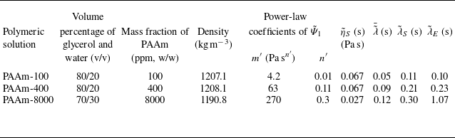
throughout all rheological tests. Rheological measurements were conducted 72h after sample preparation to ensure that thermodynamic equilibrium had been achieved. Figure 3 presents the viscosity curves of the polymeric solutions as a function of shear rate.
Viscosity curves of polymeric solutions at
 ${25}\,^\circ \textrm {C}$
.

PAAm-100 exhibited nearly constant viscosity across a broad shear rate range, while shear-thinning behaviour was observed only in PAAm-400 at shear rates below
 ${0.3}\,\textrm {s}^{-1}$
(very low shear rates). Consequently, these samples were classified as Boger fluids – viscoelastic liquids with constant viscosity. PAAm-8000 has a nonlinear pseudoplastic viscosity across all measured data points. Here, the Carreau–Yasuda equation is used to model the viscosity (
 $\tilde {\eta }$
) of this solution as a function of shear rate (
 $\tilde {\dot {\gamma }}$
):
 \begin{equation} \frac {{\tilde {\eta }}\big ({\tilde {\dot {\gamma }}}\big )-{\tilde {\eta }}_{\infty }}{{\tilde {\eta }}_{0}-{\tilde {\eta }}_{\infty }}=\frac {1}{\big (1+\big ({\tilde {\lambda }}_{\textit{CY}}\lvert {\tilde {\dot {\gamma }}}\rvert \big )^a\big )^{\frac {1-n}{a}}} ,\end{equation}
where
 ${\tilde {\eta }}_0$
and
 ${\tilde {\eta }}_\infty$
are the viscosities at the zero and infinite shear rates,
 ${\tilde {\lambda }}_{\textit{CY}}$
is the characteristic time of the model,
 $n$
is the power-law index, and
 $a$
is a parameter that characterises the transition from the Newtonian plateau to the power-law region. By curve fitting of (3.1) on the viscosity data of PAAm-8000, these constants are measured as
 ${\tilde {\eta }}_0 = {4500}\,\textrm {mpa s},\ {\tilde {\eta }}_{\infty } \approx 0,\ {\tilde {\lambda }}_{{CY}} = {4.313}\,\textrm {s},\ n = 0.646\ \text{and}\ a = 0.873$
. Highly dilute polyacrylamide solutions were also prepared to measure the intrinsic viscosity
 $ [{\tilde {\eta }} ]$
, which was estimated to be
 ${3.01}\,\textrm {l g}^{-1}$
at
 ${25}\,^\circ {\textrm {C}}$
.
The first normal stress difference is a key rheological property influencing viscoelastic flow behaviour in shear flow. Typically measured during viscosity testing, it reflects the anisotropy in the extra stress tensor resulting from the alignment of polymer chains along the streamlines under steady shear conditions. Figure 4 depicts the first normal stress difference coefficient (
 ${\tilde {\varPsi }}_1$
) of polymeric solutions versus shear rate at
 ${25}\,^\circ {\textrm {C}}$
. According to the figure,
 ${\tilde {\varPsi }}_1$
decreases with increasing shear rate for all samples. Here, this material modulus is modelled via the power-law equation:
 \begin{equation} {\tilde {\varPsi }}_1=m^\prime {\tilde {\dot {\gamma }}}^{n^\prime -2}, \end{equation}
where
 $m^\prime$
and
 $n^\prime$
represent the consistency coefficient and the power-law index of the first normal stress difference coefficient, respectively. The optimal values of
 $m^\prime$
and
 $n^\prime$
for polymeric solutions have been reported in table 2. In figure 4, the solid lines represent the fitted curves obtained from the power-law relation of (3.2). The power-law model accurately fits the data at low to moderate shear rates
 $ (\tilde {\dot {\gamma }}\lt 10 \,\mathrm{s}^{-1} )$
. At high shear rates, the power-law correlation becomes less accurate due to molecular stretching and possible onset of shear-thinning saturation, which the simple model does not capture. The nominal shear rate of the droplets of this study
 $ (\tilde {V}_\infty /2\tilde {R}\approx 0.2-7 \,\mathrm{s}^{-1} )$
falls within the fitted range, confirming the adequacy of (3.2) for the conditions studied.
First normal stress difference coefficient
 $(\tilde {\varPsi }_1)$
versus shear rate for PAAm-100, PAAm-400 and PAAm-8000 solutions at
 ${25}\,^\circ {\textrm {C}}$
. Solid lines show power-law fits applied to small and moderate shear rates
 $(\tilde {\dot {\gamma }}\lt 10 \,\mathrm{s}^{-1})$
where the data follow power-law behaviour.

Properties of the exterior phase at
 $25\,^{\circ}\mathrm{C}$
.

Frequency sweep test data of polymeric solutions at 10% strain and
 ${25}\,^\circ {\textrm {C}}$
. Here, the circle and square symbols represent
 $\tilde {G}'$
and
 $\tilde {G}''$
data points, respectively. The continuous curves indicate the results of curve fitting using the generalised Maxwell model.

3.2.3. Dynamic rheological properties
Consistent with the viscometric measurements, the oscillatory shear tests were conducted on an Anton Paar MCR 302 rheometer fitted with a 50mm cone-and-plate geometry. All rheological measurements were performed at a controlled temperature of
 ${25}\,^\circ {\textrm {C}}$
. Small-amplitude oscillatory shear (SAOS) experiments were carried out to evaluate the linear viscoelastic behaviour of the samples. Amplitude sweep tests were first conducted to determine the limits of the linear viscoelastic region (LVR), followed by frequency sweep measurements performed within this region at a constant strain amplitude. The amplitude sweep results at a low frequency (1Hz) indicated that both the storage modulus (
 $\tilde {G}'$
) and the loss modulus (
 $\tilde {G}''$
) remained constant up to approximately 40% strain, confirming linear viscoelastic behaviour in this range. Accordingly, a 10% strain was selected for the frequency sweep tests to ensure that all measurements were performed within the LVR. The frequency-sweep measurements for polymeric solutions are shown in figure 5. The circular and square symbols represent the
 $\tilde {G}'$
and
 $\tilde {G}''$
data points, respectively. For all samples, both
 $\tilde {G}'$
and
 $\tilde {G}''$
increased with angular frequency (
 $\tilde {\omega }$
), indicating typical viscoelastic liquid behaviour characterised by a transition from a viscous-dominated to an elastic-dominated response as the deformation rate increased. At low frequencies,
 $\tilde {G}''$
exceeded
 $\tilde {G}'$
, reflecting dominant viscous behaviour; however, at higher frequencies,
 $\tilde {G}'$
approached or even surpassed
 $\tilde {G}''$
, suggesting enhanced elasticity due to restricted molecular mobility and entanglement effects.
A clear dependence of the moduli on concentration was observed. The PAAm-100 solution exhibited the lowest
 $\tilde {G}'$
and
 $\tilde {G}''$
values over the entire frequency range, consistent with a predominantly liquid-like response and short relaxation times. The PAAm-400 sample displayed intermediate modulus values, indicating a moderate enhancement in elastic behaviour compared with PAAm-100. In contrast, the PAAm-8000 solution showed the highest moduli across all frequencies, with
 $\tilde {G}'$
and
 $\tilde {G}''$
increasing more rapidly with
 $\tilde {\omega }$
, signifying a more pronounced elastic network structure and slower relaxation dynamics. All results were analysed within the frequency range where
 $\tilde {G}'$
exhibited a consistent increasing trend; any decrease in
 $\tilde {G}'$
at very high frequencies was excluded, as it is attributed to the inertial effects of the measuring system.
The generalised (multi-mode) Maxwell model was employed to represent the viscoelastic behaviour of PAAm solutions and to extract their discrete relaxation spectra from frequency-sweep experiments. This model describes the material as an ensemble of several Maxwell elements connected in parallel, each consisting of a spring (elastic element) and a dashpot (viscous element). Each mode corresponds to a molecular relaxation process characterised by a specific viscosity (
 $\tilde {\eta }_i$
) and relaxation time (
 $\tilde {\lambda }_i$
). The overall viscoelastic response of the material is then obtained by summing the contributions of all modes based on the superposition of linear responses. In an oscillatory shear test, the model predicts the storage modulus (
 $\tilde {G}'$
) and loss modulus (
 $\tilde {G}''$
) as frequency-dependent functions of these parameters, given by Bird et al. (Reference Bird, Armstrong and Hassager1987):
 \begin{equation} \tilde {G}' = \sum _{i=1}^{n} \frac {\tilde {\eta }_i \tilde {\lambda }_i \tilde {\omega }^2}{1 + \tilde {\lambda }_i^2 \tilde {\omega }^2}, \end{equation}
 \begin{equation} \tilde {G}'' = \tilde {\eta }_s \tilde {\omega } + \sum _{i=1}^{n} \frac {\tilde {\eta }_i \tilde {\omega }}{1 + \tilde {\lambda }_i^2 \tilde {\omega }^2}, \end{equation}
where
 $\tilde {\eta }_s$
represents the viscosity of the Newtonian solvent,
 $\tilde {\omega }$
is the angular frequency,
 $n$
is the number of relaxation modes, and
 $\tilde {\eta }_i$
and
 $\tilde {\lambda }_i$
denote the viscosity and relaxation time of mode
 $i$
, respectively. These equations describe how the material’s elastic and viscous responses evolve with deformation frequency. To determine the set of relaxation parameters (
 $\tilde {\eta }_i$
,
 $\tilde {\lambda }_i$
), an error function (
 $f$
) was defined to quantify the difference between the model predictions and the experimental data (Bird et al. Reference Bird, Armstrong and Hassager1987):
 \begin{equation} f = \sum _{j=1}^{m} \left [ \left ( 1 - \frac {\tilde {G}'_{\textit{Model}}(\tilde {\omega }_{\!j})}{\tilde {G}'_{\textit{Data}}(\tilde {\omega }_{\!j})} \right )^2 + \left ( 1 - \frac {\tilde {G}''_{\textit{Model}}(\tilde {\omega }_{\!j})}{\tilde {G}''_{\textit{Data}}(\tilde {\omega }_{\!j})} \right )^2 \right ]\!, \end{equation}
where
 $m$
is the number of experimental data points. A hybrid genetic algorithm was employed to minimise this error function, combining the global search capability of genetic algorithms with the precision of local optimisation methods. This approach enhances convergence and avoids local minima, leading to a more accurate representation of the experimental response. The results of curve fitting using
 $n=4$
relaxation modes for PAAm-100 and PAAm-400, and
 $n=8$
modes for PAAm-8000, are presented in figure 5. The fitted curves agree well with the experimental data, confirming that the generalised Maxwell model captures the viscoelastic behaviour of the PAAm solutions over the studied frequency range. The close overlap between the predicted and measured moduli demonstrates that the model effectively represents the distribution of relaxation mechanisms within the system.
The average relaxation time constant (
 $\bar {\tilde {\lambda }}$
) of each polymeric solution was calculated from the individual relaxation times using a weighted average expression (Bird et al. Reference Bird, Armstrong and Hassager1987):
 \begin{equation} \bar {\tilde {\lambda }} = \frac {\sum _{i=1}^{n} \tilde {\eta }_i \tilde {\lambda }_i}{\sum _{i=1}^{n} \tilde {\eta }_i} .\end{equation}
The values of the longest (
 $\tilde {\lambda }_S$
) of the discrete relaxation spectrum and average relaxation times (
 $\bar {\tilde {\lambda }}$
) of polymeric samples are presented in table 2.
3.2.4. Elongational properties
Elongational viscosity was determined using a HAAKE-CaBER-2 extensional rheometer (Thermo Fisher Scientific), which is designed to characterise the transient extensional properties of dilute viscoelastic fluids such as polymer solutions. A small sample volume (approximately
 ${100}\,{\unicode{x03BC}}\textrm {l}$
) was placed between two parallel circular plates in each experiment. After forming a stable liquid bridge at a small initial gap, the upper plate was rapidly displaced to a preset final position, stretching the liquid into a cylindrical filament. The extension height was 9mm, generating a well-defined uniaxial elongation and a corresponding Hencky strain. Data point counts were 1001 for PAAm-100, 202 for PAAm-400 and 8442 for PAAm-8000. The evolution of the filament diameter over time was measured using a high-speed laser micrometer system integrated into the CaBER-2 device. The micrometer featured a spatial resolution of 0.01mm, employed a laser with a wavelength of 780nm and operated at an output power of 1.7mW. The laser beam is aligned perpendicularly to the filament and scans across its midpoint, detecting changes in light intensity as the filament thins. This non-invasive optical method enables precise, time-resolved monitoring of the filament’s minimum diameter, typically recorded at the centre of the filament, where deformation is most uniform. From the measured diameter
 $D(t)$
, the local strain rate
 ${\tilde {\dot {\varepsilon }}}({\tilde {t}})$
and transient extensional viscosity
 ${\tilde {\eta }^{+}_E}({\tilde {t}})$
were computed. The elongational viscosity is given by
 \begin{equation} {\tilde {\eta }^+_E}({\tilde {t}})=\frac {{\tilde {\tau }}_{xx}-{\tilde {\tau }}_{zz}}{{\tilde {\dot {\varepsilon }}}({\tilde {t}})}, \end{equation}
where the extensional stress
 ${\tilde {\tau }}_{xx}-{\tilde {\tau }}_{zz}$
is estimated based on the surface tension and filament geometry, and the strain rate is derived from the rate of change of the filament diameter:
 \begin{equation} {\tilde {\dot {\varepsilon }}}({\tilde {t}})=-\frac {2}{{\tilde {d}_N}}\frac {{\mathrm{d} \tilde {d}_N}}{{\mathrm{d}}{\tilde {t}}} .\end{equation}
This approach provides detailed insight into the extensional flow behaviour, including phenomena such as strain hardening and relaxation dynamics. All measurements were performed under controlled ambient conditions and the CaBER-2 device was calibrated following the manufacturer’s procedure (verification of plate alignment/displacement and laser-micrometer diameter measurement) prior to testing to ensure data accuracy. The results of these tests are presented in figure 6. As illustrated, the filament diameter decreased progressively throughout the measurement, exhibiting capillary thinning behaviour in two distinct regimes. In the initial stage of the test, the diameter decreased exponentially, reflecting the dominant extensional flow dynamics (Bazilevskii et al. Reference Bazilevskii, Entov and Rozhkov1990; Stelter et al. Reference Stelter, Brenn, Yarin, Singh and Durst2000):
 \begin{equation} {\tilde {d}}_N={\tilde {d}}_{N,0} e^{-\frac {{\tilde {t}}}{3{\tilde {\lambda }_E}}}. \end{equation}
Capillary breakup extensional rheometry profiles of polymeric solutions at
 ${25}\,^\circ {\textrm {C}}$
: (a) temporal evolution of the filament diameter; (b) elongational viscosity plotted as a function of the normalised filament diameter.

where
 ${\tilde {d}}_N$
is the instantaneous neck diameter,
 ${\tilde {d}}_{N,0}$
represents the neck diameter at the onset of the exponential thinning regime and
 ${\tilde {\lambda }}_E$
is the characteristic thinning time constant describing the rate of filament diameter reduction. The characteristic times
 ${\tilde {\lambda }}_E$
for samples PAAm-100, PAAm-400 and PAAm-8000 were determined to be 0.1, 0.23 and 1.07s, respectively.
In the second extensional regime, the filament diameter departs from the initial exponential decay as the polymer chains become highly stretched, approaching their finite (maximum) extensibility rather than being fully straightened into a taut configuration (Yarin Reference Yarin1993). At this stage, elastic stresses dominate the force balance, which slows the thinning and leads to deviations from a purely capillary-driven exponential profile. This later-time behaviour is consistent with the terminal steady elongational state described by Stelter et al. (Reference Stelter, Brenn, Yarin, Singh and Durst2002), where chains reach a maximum (but not complete) stretch and the filament thins in a nearly Newtonian manner while sustaining a very large terminal extensional viscosity, far exceeding the Newtonian Trouton ratio.
The rheological characterisation of PAAm solutions requires a direct comparison between the longest linear relaxation time (
 $\tilde {\lambda }_S$
), derived from SAOS measurements, and the extensional relaxation time (
 $\tilde {\lambda }_E$
), obtained from CaBER experiments. This comparison is essential for elucidating polymer relaxation dynamics across different concentration regimes relative to the critical overlap concentration (
 $c^*$
). For PAAm in aqueous solution, literature estimates place
 $c^*$
at approximately 600ppm (Amarouchene et al. Reference Amarouchene, Bonn, Meunier and Kellay2001; Tirtaatmadja, McKinley & Cooper-White Reference Tirtaatmadja, McKinley and Cooper-White2006; Zell et al. Reference Zell, Gier, Rafaï and Wagner2010), indicating that PAAm-100 (100ppm) and PAAm-400 (400ppm) correspond to the dilute or weakly semi-dilute regime (
 $c \leqslant c^*$
), whereas PAAm-8000 (8000ppm) lies well within the concentrated and entangled regime (Liu, Jun & Steinberg Reference Liu, Jun and Steinberg2009).
For the lower-concentration samples, PAAm-100 and PAAm-400, the
 $\tilde {\lambda }_S$
and
 $\tilde {\lambda }_E$
values are of comparable magnitude. Specifically, for PAAm-100,
 $\tilde {\lambda }_S = {0.11}\,\textrm {s}$
and
 $\tilde {\lambda }_E = {0.10}\,\textrm {s}$
; for PAAm-400,
 $\tilde {\lambda }_S = {0.21}\,\textrm {s}$
and
 $\tilde {\lambda }_E = {0.23}\,\textrm {s}$
. This close correspondence, where the ratio
 $\tilde {\lambda }_E / \tilde {\lambda }_S \approx O(1)$
, is typical of highly flexible polymer chains in the dilute state (Kolte & Szabo Reference Kolte and Szabo1999; Anna & McKinley Reference Anna and McKinley2001). The small difference between
 $\tilde {\lambda }_S$
and
 $\tilde {\lambda }_E$
in these low-concentration systems can be partially attributed to the experimental challenges associated with accurately resolving linear viscoelastic properties via SAOS, since weakly elastic solutions exhibit very small storage moduli (
 $\tilde {G}'$
) and inertia effects at higher frequencies can obscure precise determination of
 $\tilde {\lambda }_S$
(Ewoldt et al. Reference Ewoldt, Johnston and Caretta2015). A slight tendency for
 $\tilde {\lambda }_E$
to exceed
 $\tilde {\lambda }_S$
, as observed here, is commonly attributed to the self-concentration effect, where molecular chains undergo significant stretching during extensional flow, thereby enhancing intermolecular interactions even below the equilibrium
 $c^*$
(Clasen et al. Reference Clasen, Plog, Kulicke, Owens, Macosko, Scriven, Verani and McKinley2006b
).
In marked contrast, the highly concentrated PAAm-8000 solution displays a pronounced divergence between the two characteristic time scales:
 $\tilde {\lambda }_S = {0.30}\,\textrm {s}$
, whereas
 $\tilde {\lambda }_E = {1.17}\,\textrm {s}$
. This substantial difference, where
 $\tilde {\lambda }_E$
is nearly four times larger than
 $\tilde {\lambda }_S$
, is characteristic of the entangled regime, in which the CaBER measurements deviate from the simple elasto-capillary balance typically applicable to dilute polymer solutions (Anna & McKinley Reference Anna and McKinley2001). In this state,
 $\tilde {\lambda }_E$
represents the characteristic time for viscoelastic stress growth under uniaxial elongation, which is substantially amplified by increased polymer entanglement and chain connectivity. Conversely,
 $\tilde {\lambda }_S$
corresponds to the relaxation process observed under small-amplitude oscillatory deformation.
Given the experimental uncertainties in determining
 $\tilde {\lambda }_S$
for weakly elastic fluids and the fact that
 $\tilde {\lambda }_E$
directly reflects the elastic stress buildup in strong extensional flows,
 $\tilde {\lambda }_E$
is generally regarded as the more representative relaxation time for describing the dynamic response of PAAm solutions. Consequently,
 $\tilde {\lambda }_E$
is routinely used as a characteristic time constant to define key dimensionless groups governing viscoelastic flow behaviour, such as the Deborah number, the elasticity number and the Weissenberg number (Anna & McKinley Reference Anna and McKinley2001; Pilz & Brenn Reference Pilz and Brenn2007).
Finally, it is important to emphasise that the CaBER experiments were not conducted merely for rheological completeness, but to provide quantitative parameters directly relevant to the flow analysis. The extensional relaxation time (
 $\tilde {\lambda }_E$
) obtained from CaBER measurements serves as the characteristic relaxation time in the definitions of the Deborah and elasticity numbers in this study. Moreover, the steady-state elongational viscosity (
 $\tilde {\eta }_E$
) derived from the FENE-P model fitted to the CaBER data will be used in §5 for the quantitative analysis of droplet dynamics. The detailed procedure for determining
 $\tilde {\eta }_E$
is presented in Appendix C. In this way, the CaBER results establish a consistent connection between the material characterisation and the subsequent hydrodynamic interpretation discussed later in the paper.
3.3. Newtonian samples
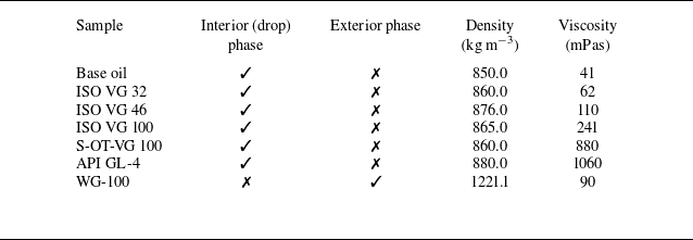
The Newtonian fluids used in this study include base oil, ISO VG 32, ISO VG 46, ISO VG 100, S-OT-VG 100, API GL-4 and WG-100. Except for WG-100, all samples were employed as the interior (drop) phase. The Newtonian fluid designated as WG-100 is a binary mixture comprising 17% water and 83% glycerol by volume (v/v), formulated to match the viscosity of the PAAm-100 Boger fluid. The above-mentioned oils are immiscible with the used polymeric solutions and WG-100, thereby enabling the formation of stable oil droplets within these continuous phases. In this context, the dynamics of oil droplets in WG-100 are compared with those in PAAm-100 to distinguish and evaluate the influence of fluid elasticity. In this study, a high-viscosity Newtonian fluid was prepared by dissolving a viscosity-enhancing additive in ISO VG 100 base oil. The additive, marketed under the name BG RF-7 Oil Treatment, is manufactured by the BG Group. When the concentration of the additive exceeds 40 wt %, the resulting mixture exhibits non-Newtonian pseudoplastic behaviour. Conversely, the fluid demonstrates approximately Newtonian behaviour at concentrations below this threshold. A solution containing 30 wt % of the additive in ISO VG 100 oil was also employed for droplet generation experiments and is hereafter referred to as S-OT-VG100. The viscosity of this formulation is approximately 3.6 times greater than that of the pure ISO VG 100 oil. The physical properties of Newtonian liquids used in this study are presented in table 3. Here, viscosity measurements were performed at
 ${25}\,^\circ {\textrm {C}}$
using an Anton Paar MCR 302 rheometer fitted with a 27mm cylindrical measuring system (spindle). As summarised in the table, although the densities of these oils are relatively similar, they span a wide range of viscosities for the interior phase, allowing for a systematic investigation of the effects of viscosity on droplet dynamics.
Properties of Newtonian fluids at
 ${25}\,^\circ {\textrm {C}}$
.

3.4. Interfacial tension
Surface tension was measured using a Theta Flex tensiometer (Biolin Scientific, Sweden) at the Experimental Thermo-Fluids Mechanics and Energy Systems (ExTENsys) Laboratory in the School of Mechanical Engineering at Pusan National University. Employing the pendant-drop method, a drop was formed and suspended from the instrument’s needle, and the surface tension was determined by analysing the radius of curvature of the drop profile.
This instrument measures the surface tension of droplets in ambient air and includes an accessory for surface tension measurements under high-pressure gas or liquid environments. The drop’s radius of curvature is determined by high-speed imaging of the pendant drop and subsequent analysis using the computer software linked to the tensiometer. It can measure surface tension values from
 ${0}\,\rm {mN\,m}^{-1}$
to
 ${2000}\,\rm {mN \,m}^{-1}$
with an accuracy of
 $\pm$
0.01
 $\rm {mN \,m}^{-1}$
to
 $\pm 0.1\,\rm {mN \,m}^{-1}$
. The tensiometer’s high-speed camera has a maximum image size of
 $1264\times 1984$
pixels (
 $\approx$
2.5 megapixels) and captures images at up to 3009 frames per second at this setting. The spatial calibration (
 ${\unicode{x03BC}}$
m pixel-1) depends on the selected magnification/field of view and was determined within the OneAttension software prior to analysis. For the Theta Flex, the adjustable field of view (1.44–32.3mm diagonal) corresponds to an effective scale of roughly 0.6–14
 ${\unicode{x03BC}}$
m pixel−1, depending on magnification. The measured interfacial tension coefficients,
 $\tilde {\sigma }$
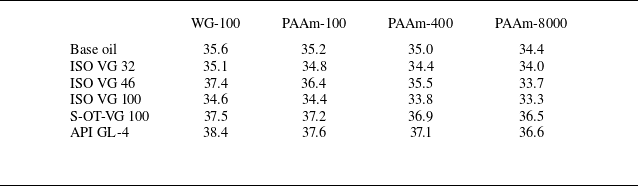
, of the samples are reported in table 4. According to the table,
 $\tilde {\sigma }$
varies slightly, ranging from
 ${30.5}\,\rm {mN\, m}^{-1}$
to
 ${37.5}\,\rm {mN\, m}^{-1}$
. The amounts of water and glycerol in the exterior phase do not change significantly, and PAA has little effect on the interfacial tension. Additionally, since the interior (drop) phase is based on mineral oil, the overall variation in
 $\sigma$
remains limited.
Interfacial tension coefficient (
 $\textrm {mN m}^{-1}$
) at
 ${25}\,^\circ {\textrm {C}}$
.

3.5. Visualisation
For performing the shadowgraphy test, a prismatic tank with a volume of approximately 18l is filled with the exterior fluid (the medium surrounding the droplet). Before starting the experiment, it is essential to capture a reference image (with no droplet present) of the set-up. By opening the injection valves, the Newtonian oil (drop phase) is injected into the tank using a syringe pump. The flow rate can be easily adjusted using the speed of the syringe pump. By adjusting the projector light and the camera software settings, imaging is initiated. The camera is set to cover a height of 81mm, and imaging starts from an injection height of 6cm. Due to the very high viscosity of the exterior fluid, droplets usually reach their maximum size quickly within the imaging area. The dimensions of the captured images are
 $800\times 1280$
pixels, so the size of each pixel is approximately 0.0633mm. Also, considering the high viscosity of the exterior fluid, a very high imaging speed is not necessary and a frame rate of 300 frames per second is sufficient for these tests.
After data acquisition, an image processing code is required to analyse the shadowgraphy results. The necessary codes for analysing the dynamics of droplets have been written in MATLAB, primarily relying on the Image Processing Toolbox of this software. The image-processing procedure used in this study is identical for all droplets analysed. Each recorded frame is processed to extract both geometrical parameters, such as the surface profile, centre-of-volume position, aspect ratio and droplet volume, and kinematical parameters, particularly the terminal velocity. In the MATLAB implementation, each frame and its corresponding background reference image are imported as matrices. Subtracting the reference matrix from the frame isolates the droplet from the background, and the resulting difference image is binarised to distinguish the droplet from the surrounding fluid clearly. Any noise present at this stage is removed using appropriate filtering techniques.
Connected regions in the binary image are then identified using the ‘regionprops’ function and the largest region is selected as the droplet. This region is isolated, and a boundary-detection algorithm is applied to locate the interface between the droplet and the exterior fluid. The extracted boundary coordinates are stored as a two-dimensional array representing the droplet’s geometric profile. From this geometric profile, all relevant shape parameters are computed. Applying the same procedure to each frame allows accurate determination of droplet shape evolution and terminal velocity across all experiments.
Additionally, by tracking the instantaneous position of the centre of volume in each frame relative to a reference system, the terminal velocity of the droplet can be estimated. This analysis has an approximate error of one or two pixels. A line is fitted to the centre-of-volume trajectory to derive the terminal velocity of the droplet. Obviously, the slope of this line represents the terminal velocity. As an example, figure 7 presents the result of image processing for the vertical trajectory of the droplet’s centre of volume of an ISO VG 32 oil droplet released from a 3/8-inch nozzle into a PAAm-8000 solution over 1000 frames. The suitable agreement between the experimental data and the fitted linear trend indicates that the droplet has entered the terminal velocity regime. The terminal velocity is also estimated to be approximately 4.82mms−1.
Vertical position of the centre of volume of an ISO VG 32 oil droplet released from a 3/8-inch nozzle into a PAAm-8000 solution, plotted as a function of time over 1000 frames.

The accuracy of the terminal-velocity determination was carefully evaluated based on the optical resolution, imaging rate and data-processing precision. The vertical position of the droplet’s centre of volume was tracked with subpixel accuracy, yielding a positional uncertainty of approximately 0.10px to 0.15px (0.006 to 0.010mm) within the calibrated imaging field (0.0633mm px
 $^{-1}$
). Linear fitting of the position–time data over steady intervals of at least 60 frames to 100 frames (0.2s to 0.33s) provided the terminal velocity with a standard error of 0.2% to 0.5%. The total uncertainty, including spatial calibration (
 ${{\lt} 0.5}{\,\%}$
) and frame-rate precision (1/300s), remains below
 ${2}{\,\%}$
. Figure 7 demonstrates the linearity of the droplet trajectory over 1000 frames, confirming that the droplets fully reached their terminal regime and validating the reliability of the velocity measurement. The low Reynolds number (
 $\textit{Re} \lt 1$
) ensures steady motion, so the reported terminal velocities are quantitatively accurate and reproducible with an uncertainty smaller than
 ${2}{\,\%}$
.
The steadiness of droplet motion was carefully verified in all experiments to confirm that each droplet reached a genuine terminal regime before data analysis. The imaging system was configured to cover a vertical distance of 81mm and the field of view was positioned so that recording began at least 8cm above the droplet injection point. This arrangement ensured that the droplet was fully detached and had already entered a stable rising regime before entering the imaging area, thereby eliminating any transient effects associated with droplet formation or nozzle disturbance.
The steadiness of the motion is illustrated in figure 7, which shows the vertical trajectory of the droplet’s centre of volume over 1000 consecutive frames for a Newtonian droplet in the highly viscous PAAm-8000 solution. The excellent linear correlation between position and time demonstrates that the droplet had completely reached its terminal velocity within the recorded region. The fitted line corresponds to a terminal velocity of approximately
 ${4.82}\,\textrm {mm s}^{-1}$
and the residual scatter of the data remains within the subpixel uncertainty range, confirming highly stable motion. In the less viscous continuous phases, a slightly longer acceleration stage was observed immediately after droplet formation, but the droplets reached a steady terminal velocity shortly after entering the imaging field. It is also important to note that, unlike gas bubbles, the droplets used in this study are incompressible; thus, compressibility-related transient effects that often contribute to unsteady bubble motion are absent. Furthermore, the viscosity of these droplets is several orders of magnitude higher than that of gas bubbles, providing strong internal hydrodynamic damping that stabilises the motion. Because the density difference between the droplet and the surrounding solution is much smaller than in the case of gas bubbles, the buoyancy-driven acceleration is also reduced. These lead to weaker inertial transients after detachment, which contribute to the overall steadiness of the droplet motion. Combined with the much larger internal viscosity of the droplets, these factors strongly stabilise the rising trajectory. In all experiments, the droplet motion remained vertically aligned, with no detectable oscillations, lateral displacements or path instabilities throughout the observed trajectory.
4. Results and discussion
4.1. Analytical results
In this section, the results obtained from the analytical solution using the perturbation method are presented. These results can be used to evaluate the physical reasons underlying the various phenomena observed in the experimental results section (§5).
Terminal velocity (left axis) and Reynolds number (right axis) of Newtonian drops as functions of droplet volume at
 ${k}=1$
. Solid lines, present study; open circles, data of Taylor & Acrivos (Reference Taylor and Acrivos1964).

4.1.1. Validation
To validate our analytical solution, we compared it with the classical results of Taylor & Acrivos (Reference Taylor and Acrivos1964), which describe the upward motion of Newtonian droplets rising through a Newtonian fluid in the inertial regime. By setting the Deborah number to zero, our model reduces to this classical Newtonian case, enabling a direct and meaningful comparison. Figure 8 shows the terminal velocity (left ordinate) and Re (right ordinate) as a function of droplet volume, with our analytical predictions (solid line) plotted alongside the reference data (open circles). The agreement between the two is excellent across the entire range of volumes considered (20–180
 $\textrm {mm}^{3}$
), with relative deviations remaining below 2%. For instance, at a droplet volume of 100
 $\textrm {mm}^{3}$
, our model predicts a terminal velocity of approximately 31.7mms−1, which is comparable to the
 ${31.4}\,\textrm {mm s}^{-1}$
reported in the reference. The results also confirm the expected physical behaviour: the increase of terminal velocity with drop size reflects the balance between buoyancy and the total hydrodynamic drag. At low
 $\textit{Re}$
, the drag arises from both pressure and viscous stresses of comparable order, and equilibrium of drag with buoyancy yields
 $\tilde V_\infty \sim \Delta \tilde \rho \, g\, \tilde R^2/\tilde \eta _{\textit {e,0}}$
, with
 $\Delta \tilde \rho =\tilde \rho _{\textit {e}}-\tilde \rho _{\textit {i}}$
(Hadamard–Rybczynski/Stokes scaling, with a prefactor depending on
 ${k}$
). Therefore, larger drops, having buoyancy growing as
 $\tilde {R}^3$
, attain higher terminal velocities through this force balance. In the inertial regime, this enhanced driving force leads to a higher steady rising speed, as inertial effects outweigh viscous resistance.
Deformation of ISO VG 32 droplets moving through PAAm-8000 (viscoelastic) medium, (a)
 ${\textit{De}}=0.29 (\tilde {\varOmega }=32.56\,\mathrm{mm}^3)$
, (b)
 ${\textit{De}}=0.37 (\tilde {\varOmega }=56.26\,\mathrm{mm}^3)$
and (c)
 ${\textit{De}}=0.44 (\tilde {\varOmega }=98.10\,\mathrm{mm}^3)$
. The first row shows the experimental images, whereas the second row shows the analytical results. The reported volumes correspond to the experimental images.

Deformation of ISO VG 46 droplets moving in WG-100 (Newtonian) medium: (a)
 ; (b)
 $\textit{Re}=1.08 \,(\tilde {\varOmega }=33.3\,\mathrm{mm}^3)$
; and (c)
 $\textit{Re}=1.87 \,(\tilde {\varOmega }=60.7\,\mathrm{mm}^3)$
. The first row shows the experimental images, whereas the second row shows the analytical results. The reported volumes correspond to the experimental images.

This strong quantitative agreement with a well-established benchmark demonstrates the robustness of our model in the Newtonian limit. It builds a reliable foundation for exploring viscoelastic effects at finite Deborah numbers.
Figure 9 shows the shapes of ISO VG 32 droplets moving through PAAm-8000 (a viscoelastic fluid) for small volumes (up to
 $124\,\mathrm{mm}^3$
), based on both analytical and experimental results. To quantitatively assess droplet shape, the diameter ratio (
 $\chi$
) is used, defined as the ratio of the horizontal to vertical droplet diameters (
 $\chi =\tilde {D}_x/\tilde {D}_y$
). Values of
 $\chi$
differing from unity indicate deformation from a spherical shape, with the extent and direction of deviation reflecting the influence of fluid rheology. The droplet shape remains nearly spherical (with
 $\chi =0.95$
) at
 ${\textit{De}}=0.29$
, due to the small volume of the droplet and the dominant effect of interfacial tension. However, as the droplet volume and Deborah number increase, the diameter ratio decreases and the droplets become increasingly elongated in the direction of motion. This deformation arises from the elasticity of the surrounding fluid, particularly its strain-hardening elongational viscosity, which resists the upward motion of the droplet. According to the figure, there is good agreement between the two sets of results, confirming the accuracy of the analytical solution for small perturbation parameters.
Comparison of analytical predictions and experimental measurements of terminal velocity versus droplet volume for ISO VG 32 droplets rising in PAAm-8000 medium.

Figure 10 presents the shapes of ISO VG 46 oil droplets in WG-100 media, based on both analytical predictions and experimental observations. In this case, the surrounding fluid (WG-100) is Newtonian. Unlike the behaviour shown in figure 9, the droplets progressively flatten along the vertical axis as their volume increases. The Bond number,
 ${Bo}= (\tilde {\rho }_e-\tilde {\rho }_i ) \tilde {g} \tilde {R}^2/\tilde {\sigma }$
, increases with droplet size, indicating that gravitational deformation becomes more pronounced. Although viscous forces suppress large shape variations at low Reynolds numbers, the increasing imbalance between buoyancy and interfacial tension leads to greater vertical flattening. As a result, larger droplets develop oblate shapes, reflected in diameter ratios greater than unity. As shown in figure 10, the analytical solution accurately reproduces the observed droplet deformations.
Another verification case is the terminal velocity diagram versus the volume for ISO VG 32 droplets rising in PAAm-8000. The corresponding results from the analytical solution and experimental observations are shown in figure 11. As illustrated, the analytical solution provides a reasonable prediction of the terminal velocity in the subcritical regime. The observed deviations in this regime can be attributed to the use of a single-mode Giesekus constitutive equation, which cannot fully capture all the rheological properties of the polymeric solution. The accuracy of the prediction in the subcritical regime could be further improved by employing multi-mode nonlinear constitutive equations, which can represent a more complete set of rheological properties, including viscometric functions, discrete relaxation spectra, elongational viscosity and related material moduli. The terminal velocity predicted by the analytical solution shows no discontinuity over the studied range due to the linearisation and axisymmetric assumptions, indicating a continuous curve and demonstrating that the model captures the trends in deformation and stress without exhibiting velocity jumps (see figure 11). According to Bothe et al. (Reference Bothe, Niethammer, Pilz and Brenn2022), full three-dimensional nonlinear modelling is required to capture velocity jumps in bubbles. Similar simulations are therefore expected to be necessary to model velocity jumps and the supercritical regimes in droplets.
4.1.2. Deformation of drop
Figure 12 illustrates the effect of the Reynolds number on the deformation behaviour of Newtonian fluid droplets rising through a Newtonian medium, in the absence of elasticity effects (
 ${\textit{De}}=0$
). At low Reynolds numbers, characteristic of the creeping or Stokes flow regime, the motion is dominated by viscous forces and inertial effects are negligible. In this regime, the interfacial tension between the droplet and the surrounding fluid plays a dominant role, maintaining a configuration with a minimal surface area. As a result, the droplet retains a nearly perfect spherical shape, which corresponds to the shape with the lowest surface energy.
As the Reynolds number increases, inertial forces become significant compared with viscous forces. These inertial effects introduce asymmetries in the pressure and velocity fields around the rising droplet. Specifically, the flow tends to accelerate around the equator of the droplet, and decelerate near the front and rear stagnation points, generating a pressure differential. This differential leads to a net stress distribution that compresses the droplet vertically and stretches it radially, resulting in an oblate (flattened) shape.
The extent of this deformation increases with Reynolds number because the inertial forces continue to grow in relation to interfacial tension and viscous forces. The degree of flattening is thus a balance between the droplet’s interfacial tension, which resists deformation by trying to maintain a spherical shape, and the dynamic pressure variations caused by inertia, which favour deformation. In this purely Newtonian system (
 ${\textit{De}}=0$
), the deformation is solely attributed to the increasing dominance of inertia over interfacial tension and viscous stresses as
 $\textit{Re}$
increases.
Our observations align with the findings of Tsamopoulos et al. (Reference Tsamopoulos, Dimakopoulos, Chatzidai, Karapetsas and Pavlidis2008), confirming that the balance of buoyancy, viscous stresses and surface tension dictates droplet deformation, with larger droplets adopting increasingly oblate shapes.
Streamlines (black) overlaid on a colourmap of the flow-type parameter
 $\xi$
for a Newtonian droplet rising in a Newtonian ambient, in the absence of elasticity effects (
 ${\textit{De}}=0$
). The colourmap shows
 $\xi \in [-1,1]$
(dimensionless):
 $\xi =-1$
solid-body rotation,
 $\xi =0$
simple shear and
 $\xi =1$
pure extension (see text for definition via
 $\unicode{x1D63F}$
and
 $\boldsymbol{\varOmega }$
). Panels are ordered by increasing
 $\textit{Re}$
(left to right; values annotated in the panels) at fixed
 ${\textit{Ca}}=0.5$
and viscosity ratio
 ${k}=1$
; streamlines and
 $\xi$
are shown at the steady (terminal) rising state, and the colourbar is labelled
 $\xi$
.

Figure 13 illustrates the influence of the Deborah number on the deformation behaviour of Newtonian droplets rising in viscoelastic surrounding fluids. As
 $\textit{De}$
increases, elastic stresses within the viscoelastic medium begin to dominate. When a droplet rises, it displaces the surrounding viscoelastic fluid, which responds not just with instantaneous viscous resistance, but also with time-dependent elastic recoil. This recoil effect generates normal stresses along the direction of motion (the vertical axis), effectively ‘pulling’ on the droplet in the direction of ascent – an elastic-recoil mechanism established for bubbles via detailed numerical continuation and analysis of the velocity discontinuity (Fraggedakis et al. Reference Fraggedakis, Pavlidis, Dimakopoulos and Tsamopoulos2016) and succinctly reviewed by Zenit & Feng (Reference Zenit and Feng2018).
These normal stresses oppose radial spreading and instead promote axial elongation, leading to a prolate (elongated) shape. This is in contrast to the oblate deformation seen in Newtonian fluids under inertial conditions, where lateral spreading dominates. In viscoelastic media, the stored elastic energy around the droplet tends to stretch it vertically and the degree of this prolate deformation increases with
 $\textit{De}$
, as the fluid’s ability to store and release elastic energy becomes stronger. Thus, the observed prolate shape results from a balance between interfacial tension, which favours spherical shapes, and the viscoelastic normal stresses, which drive axial elongation. The stronger the elastic response (higher
 $\textit{De}$
), the more pronounced the vertical stretching becomes.
Streamlines (black) overlaid on a colourmap of the flow-type parameter
 $\xi$
for a Newtonian droplet rising in a viscoelastic ambient (Giesekus). The colourmap shows
 $\xi \in [-1,1]$
(dimensionless):
 $\xi =-1$
solid-body rotation,
 $\xi =0$
simple shear and
 $\xi =1$
pure extension (see text for definition via
 $\unicode{x1D63F}$
and
 $\boldsymbol{\varOmega }$
). Panels correspond to Deborah numbers increasing left to right (values annotated in the panels) at fixed
 $\textit{Re}=0.5$
,
 ${\textit{Ca}}=0.5$
,
 $\alpha =0.2$
,
 $\beta =0.5$
and
 ${k}=1$
; streamlines and
 $\xi$
are shown at the steady (terminal) rising state, and the colourbar is labelled
 $\xi$
.

Next, we further analyse the influence of normal stresses on droplet deformation. The flow-type parameter,
 $\xi$
, serves as a key indicator for describing the kinematic nature of the flow field. It is defined as
 \begin{equation} \xi =\frac {\left \|\unicode{x1D63F}_{\!j}\right \|-\left \|\boldsymbol{\varOmega }_{\!j}\right \|}{\left \|\unicode{x1D63F}_{\!j}\right \|+\left \|\boldsymbol{\varOmega }_{\!j}\right \|},\quad j=i, e, \end{equation}
where
 $ \|\unicode{x1D63F}_{\!j} \|$
and
 $\|\boldsymbol{\varOmega }_{\!j}\|$
denote the magnitudes (norms) of the deformation rate and vorticity tensors, respectively:
 \begin{equation} \begin{array}{ll} \unicode{x1D63F}_{\!j}=\dfrac {1}{2}\big(\boldsymbol{\nabla } \boldsymbol{v}_{\!j}+\boldsymbol{\nabla } \boldsymbol{v}_{\!j}^{{T}}\big), \quad \boldsymbol{\varOmega }_{\!j}=\dfrac {1}{2}\big(\boldsymbol{\nabla } \boldsymbol{v}_{\!j}-\boldsymbol{\nabla } \boldsymbol{v}_{\!j}^{{T}}\big), & \\ \left \|\unicode{x1D63F}_{\!j}\right \|=\left (\frac {\unicode{x1D63F}_{\!j}: \unicode{x1D63F}_{\!j}}{2}\right )^{\frac {1}{2}}, \quad \left \|\boldsymbol{\varOmega }_{\!j}\right \|=\left (\frac {\boldsymbol{\varOmega }_{\!j}: \boldsymbol{\varOmega }_{\!j}}{2}\right )^{\frac {1}{2}}, & j=i, e .\end{array} \end{equation}
The flow-type parameter is a dimensionless quantity ranging from
 $-1$
to 1, where
 $\xi =-1$
represents a solid-body rotational flow,
 $\xi =1$
corresponds to a pure extensional flow and
 $\xi =0$
indicates a simple shear flow.
Contours of the
 $\xi$
at various Reynolds and Deborah numbers are presented in figures 12 and 13. According to the figures, the flow is purely extensional near the droplet’s poles, around the front and rear stagnation points, whereas shear flow occurs around the droplet’s equatorial interface. When the surrounding fluid is viscoelastic (figure 13), it exhibits strong strain-hardening under extensional flow, meaning its resistance to stretching increases with deformation. As the droplet rises, elongational flow develops near both the front and rear stagnation points. At the front, the external fluid decelerates and compresses against the droplet, while at the rear, it reconverges and pulls in towards the wake. These flow conditions generate strong elastic normal stresses that act along the vertical axis, effectively stretching the droplet in the direction of motion and resulting in a pronounced prolate deformation. In parallel, the viscoelastic response to shear flow along the equatorial interface generates a strong first normal stress difference,
 $N_1$
, which acts in the plane perpendicular to the direction of motion. If sufficiently large,
 $N_1$
can exert additional elastic forces that influence the droplet shape, either opposing or reinforcing the deformation caused by the extensional stresses. This highlights the importance of considering both elongational and shear-induced elastic stresses when analysing droplet deformation in viscoelastic environments.
The analytical framework, which relies on linearisation, perturbation techniques and mass-conserving assumptions, is unable to reproduce the convex-to-concave interface transition, the small but inevitable mass loss at the tail or the teardrop-like shapes observed in the experiments. These phenomena occur near singular regions where extreme gradients in the flow and stress fields drive behaviours that diverge to infinity, rendering them beyond the validity of the classical prolate solution. Therefore, the analytical model should be regarded primarily as a theoretical guideline supporting the arguments presented by Bothe et al. (Reference Bothe, Niethammer, Pilz and Brenn2022), rather than as a tool for capturing such localised experimental features.
Angular distributions of the radial normal stress component of exterior fluid,
 $(\tau _e)_{rr}$
, for different Deborah numbers at
 $\textit{Re}=0.5,\,{\textit{Ca}}=0.5,\,\alpha =0.2,\,\beta =0.5,\,{k}=1$
.

4.1.3. Normal stress distribution at the interface
Figure 14 shows the angular distribution of the radial normal stress component
 $ (\tau _e )_{rr}$
in the exterior viscoelastic fluid surrounding a Newtonian drop rising due to buoyancy. The results correspond to Deborah numbers
 ${\textit{De}}=0.2, 0.6, 1.2$
, with the other dimensionless parameters held fixed at
 $\textit{Re}=0.5,\,{\textit{Ca}}=0.5,\,\alpha =0.2,\,\beta =0.5\,\text{and}\,{k}=1$
. The angular coordinate
 $\theta$
, measured from the front stagnation point (
 $\theta = {0}^{\circ }$
) to the rear stagnation point (
 $\theta = {180}^{\circ }$
), represents the distribution of stress along the interface of the drop. The radial normal stress component exhibits an antisymmetric pattern with respect to the equator (
 $\theta = {90}^{\circ }$
). It is negative near the front stagnation point and positive near the rear, indicating a compressive normal stress upstream and an extensional normal stress downstream.
This stress distribution arises from the interaction between the flow-induced deformation and the elastic response of the surrounding fluid. As the drop rises, the viscoelastic fluid undergoes extensional deformation near the stagnation points. At the front, fluid elements decelerate and compress against the drop interface, resulting in the buildup of compressive radial normal stresses due to the stretching and orientation of polymer chains. In contrast, at the rear, the fluid accelerates and stretches away from the interface, resulting in extensional radial normal stresses associated with elastic recovery. The magnitude of these stresses increases with the Deborah number, reflecting the increasing influence of fluid elasticity relative to the flow time scale.
Angular distributions of the exterior-fluid polar (
 $\theta$
-direction) normal stress component,
 $(\tau _e)_{\theta \theta }$
, for different Deborah numbers at
 $\textit{Re}=0.5,\,{\textit{Ca}}=0.5,\,\alpha =0.2,\,\beta =0.5,\,{k}=1$
.

Quantitatively, the radial normal stress increases monotonically with
 $\theta$
and the range of stress becomes broader as the Deborah number increases. For
 ${\textit{De}}=0.2$
, the stress ranges from approximately
 $-1.45$
to 1.3; for
 ${\textit{De}}=0.6$
, from
 $-1.25$
to 1.5; and for
 ${\textit{De}}=1.2$
, from
 $-1.1$
to 1.75. The enhancement in both compressive and extensional stress magnitudes with increasing De leads to a greater normal stress imbalance across the drop interface. This imbalance generates a net elastic force aligned with the vertical axis of motion, promoting elongation of the drop in the direction of ascent. The result is a prolate deformation driven primarily by the normal stress anisotropy induced by the viscoelastic matrix. The observed stress distribution plays a critical role in the interfacial dynamics of the drop. While interfacial tension resists deformation, the normal stress differences imposed by the surrounding fluid can dominate when elastic effects are strong. The radial normal stress component, in particular, contributes directly to the axial elongation by compressing the front and stretching the rear of the drop. This mechanism explains the deformation behaviour observed in viscoelastic environments. It highlights the central role of elasticity, as characterised by the Deborah number, in controlling drop morphology during motion through complex fluids.
Figures 15 and 16 present the angular distributions of the exterior-fluid polar (
 $\theta$
-direction) normal stress component,
 $\tau _{{e,}\theta \theta }$
, and the hoop (azimuthal) normal stress component,
 $\tau _{{e,}\phi \phi }$
, at different Deborah numbers. These figures highlight how increasing fluid elasticity alters both the magnitude and spatial distribution of these normal stress components along the drop interface. In figure 15, the polar (
 $\theta$
-direction) normal stress component,
 $ (\tau _e )_{\theta \theta }$
, which represents the elastic resistance to deformation in the polar direction, increases significantly with increasing Deborah number. At
 ${\textit{De}}=0.2$
, the stress magnitude is relatively small and the peak occurs near
 $\theta \approx {75}^{\circ }$
. As
 $\textit{De}$
increases to 0.6 and 1.2, the peak stress becomes much larger and shifts towards the rear of the drop, reaching a maximum near
 $\theta = {93}^{\circ }$
for the highest Deborah number. This rearward shift indicates that the region of greatest polymeric stretching migrates towards the rear stagnation zone as elasticity strengthens. The increase in stress is nonlinear, and this behaviour arises from the cumulative effect of fluid memory, inertial straining and local geometry. The drop deformation plays a critical role in modifying the local flow field and stress orientation. As the rear of the drop elongates under the influence of viscoelastic normal stresses, the surface kinematics promote enhanced meridional extension in that region, which in turn leads to increased stress concentration.
Angular distributions of the hoop stress component of exterior fluid,
 $(\tau _e)_{\phi \phi }$
, for different Deborah numbers at
 $\textit{Re}=0.5,\,{\textit{Ca}}=0.5,\,\alpha =0.2,\,\beta =0.5,\,{k}=1$
.

Figure 16 shows the hoop (azimuthal) normal stress component,
 $ (\tau _e )_{\phi \phi }$
, which reflects the elastic tension in the circumferential direction around the axis of symmetry. Although this stress component is generally smaller in magnitude than the polar (
 $\theta$
-direction) component, it exhibits the same qualitative behaviour: an increase in magnitude and a rearward shift in the location of its maximum as Deborah number increases. For
 ${\textit{De}}=0.2$
, the stress peak is broad and less distinct, occurring near
 $\theta \approx {75}^{\circ }$
. In contrast, for
 ${\textit{De}}=1.2$
, the peak becomes sharper and shifts to
 $\theta \approx {93}^{\circ }$
. The growth of the hoop stress highlights the increasing circumferential resistance of the polymeric fluid, even in axisymmetric flow. As the drop deforms, the surface curvature changes in a way that amplifies circumferential straining near the rear, reinforcing the buildup of azimuthal stress.
Angular distributions of the (a) polar,
 $(\tau _e)_{\theta \theta }$
, and (b) hoop,
 $(\tau _e)_{\phi \phi }$
, stress component of exterior fluid (PAAm-8000) for ISO VG 32 droplets at
 ${\textit{De}}=0.29$
 $(\tilde {\varOmega }=32.56\,\mathrm{mm}^3)$
,
 ${\textit{De}}=0.37$
 $(\tilde {\varOmega }=56.26\,\mathrm{mm}^3)$
and
 ${\textit{De}}=0.44$
 $(\tilde {\varOmega }=98.10\,\mathrm{mm}^3)$
.

The results collectively demonstrate that viscoelastic normal stresses become more pronounced and more localised with increasing elasticity, particularly in the rear hemisphere of the deformed drop. The interplay between weak inertia, fluid elasticity and shape deformation results in a complex yet systematic redistribution of stress around the interface. Although the velocity field remains continuous in this regime, the strong amplification and rearward migration of both normal stress components indicate the emergence of localised regions where viscoelastic effects increasingly influence the momentum balance. This stress localisation near the rear is often a precursor to more pronounced nonlinear behaviours observed at higher elasticity numbers, such as velocity jumps or the formation of thin stress boundary layers. While the axisymmetric nature of the present analytical solution does not permit the explicit resolution of such discontinuities, it effectively captures the underlying mechanisms (particularly the stress growth and redistribution) that foreshadow these transitions. Moreover, the inclusion of drop deformation in the analysis proves essential, as it alters the strain-rate field and flow geometry in a manner that significantly shapes the stress profile, enabling a detailed representation of the early stages of elastic stress focusing and flow evolution.
The angular distributions of the polar,
 $\tau _{e,\theta \theta }$
, and hoop,
 $\tau _{e,\phi \phi }$
, stress components for ISO VG 32 droplets rising in PAAm-8000 media are also presented based on the analytical solution (see figure 17). Although these results correspond to the subcritical regime, they illustrate the influence of the surrounding fluid’s elasticity on droplet deformation and, in particular, on the flow transition. As shown in the figures, both normal stress components increase, and their maxima shift towards the rear of the droplet as the Deborah number increases. Similar phenomena have been reported by Bothe et al. (Reference Bothe, Niethammer, Pilz and Brenn2022) for bubbles rising in viscoelastic fluids, where they attributed the observed velocity jump and flow transition to these effects. In the experimental section, these analytical results are referenced to interpret the mechanisms underlying the flow transition and the velocity jump for ISO VG 32 droplets rising in PAAm-8000.
Figure 18 shows the trace of the stress tensor in the surrounding viscoelastic fluid for a buoyancy-driven Newtonian droplet: (a) for different Deborah numbers at
 , and
 ${k}=1$
; and (b) for experimentally relevant conditions at
 ${\textit{De}}=0.29,\,0.37$
and 0.44 corresponding to ISO VG 32 droplets rising in PAAm-8000. The stress distribution along the interface, parametrised by the angular coordinate
 $\theta$
, exhibits an antisymmetric structure about the equator (
 $\theta =90^\circ$
), with negative values near the front stagnation point and positive values towards the rear. These features correspond to compressive and extensional elastic stresses, respectively, indicating distinct polymer deformation states in the leading and trailing regions of the droplet.
Trace of the stress tensor of the exterior fluid for different Deborah numbers at (a)
 ; and (b)
 ${\textit{De}}=0.29$
 $(\tilde {\varOmega }=32.56\,\mathrm{mm}^3)$
,
 ${\textit{De}}=0.37$
 $(\tilde {\varOmega }=56.26\,\mathrm{mm}^3)$
and
 ${\textit{De}}=0.44$
 $(\tilde {\varOmega }=98.10\,\mathrm{mm}^3)$
. Panel (b) corresponds to ISO VG 32 droplets rising in PAAm-8000.

In figure 18(a), increasing the Deborah number results in a systematic increase in the magnitude of the trace across most of the interface. Near the front stagnation zone, the trace becomes less negative with increasing De, suggesting partial stress relaxation. In contrast, towards the rear, the trace becomes increasingly positive, revealing stronger extensional polymer stretching and enhanced elastic energy storage. The gradient of the distribution with respect to
 $\theta$
also steepens with elasticity, indicating a more pronounced polarisation of elastic stresses between the front and rear of the droplet. A similar tendency is observed in figure 18(b) for the experimentally relevant Deborah numbers: although the stress range is narrower, the curves shift upward with increasing De, confirming that even moderate elasticity in PAAm-8000 significantly modifies the stress field. The effect is most pronounced near the stagnation regions, where polymer deformation is dominant, whereas the curves nearly collapse around the equatorial zone. In conclusion, figure 18 shows that the trace of the stress tensor increases with the Deborah number under both idealised and experimental conditions, reflecting stronger elastic stress accumulation and polymer stretching in the surrounding viscoelastic fluid as elasticity increases.
5. Experimental results
This section presents laboratory observations. As the primary aim of this study is to investigate droplet shape and motion in viscoelastic media, we begin by comparing the shapes of Newtonian droplets rising in both Newtonian and viscoelastic fluids. The influence of key parameters (including the droplet volume, elasticity and viscosity ratio) on droplet shape is then analysed. Finally, the dynamics of droplet motion in Newtonian and viscoelastic environments are compared.
5.1. Drop dynamics in Newtonian and dilute polymeric solutions
5.1.1. Drop shape
The surrounding fluid plays a crucial role in determining both the shape of a moving droplet and the flow dynamics around it. A comparison of recorded images of rising droplets in Newtonian and viscoelastic media reveals notable differences in droplet morphology. To quantitatively assess droplet shape, the diameter ratio (
 $\chi$
) is used, defined as the ratio of the horizontal to vertical droplet diameters (
 $\chi =D_x/D_y$
). Values of
 $\chi$
differing from unity indicate deformation from a spherical shape, with the extent and direction of deviation reflecting the influence of fluid rheology. Initially, the influence of different parameters on the droplet shape is examined.
A. Effect of drop volume
As expected, Newtonian droplets rising in a Newtonian medium exhibit minimal deviation from sphericity at low Reynolds numbers. With increasing droplet volume, however, the shape gradually transitions into a moderately flattened sphere. Figure 19 presents recorded images of ISO VG 46 oil droplets rising in the Newtonian fluid WG-100. As the droplet volume increases, the shape becomes increasingly oblate, corresponding to diameter ratios greater than unity. The observed transition in droplet shape with increasing volume can be attributed to the interplay between interfacial tension, buoyancy, inertial and viscous forces. For small droplets, interfacial tension dominates, maintaining a nearly spherical shape by minimising surface area and resisting deformation through Laplace pressure. As droplet volume increases, buoyant forces grow, leading to higher rise velocities and greater inertial effects. This results in increased dynamic pressure differences around the droplet, particularly between the front and rear.
Additionally, the Bond number – which quantifies the relative influence of buoyancy to interfacial tension – increases with droplet size, indicating that gravitational deformation becomes more significant. While viscous forces continue to dampen shape changes at low Reynolds numbers, the growing imbalance between buoyancy and interfacial tension causes the droplet to flatten along its vertical axis. Consequently, larger droplets exhibit oblate shapes, reflected in diameter ratios greater than unity.
Shape of ISO VG 46 oil droplets in WG-100 (Newtonian) medium at different volumes.

The viscosity of the droplet itself also influences the extent of droplet deformation during its rise. As the internal viscosity increases, the droplet exhibits greater resistance to deformation due to enhanced internal viscous dissipation, which suppresses internal circulation and dampens shape changes. This internal resistance reduces the droplet’s ability to respond dynamically to external stresses such as buoyancy and viscous drag from the surrounding fluid. Additionally, a higher viscosity ratio between the droplet and the surrounding medium alters the interfacial stress balance, leading to a reduction in the net deformation forces acting on the droplet. Consequently, droplets with higher internal viscosity tend to retain a more spherical shape, even as their volume increases, and exhibit lower diameter ratios compared with less viscous counterparts under similar conditions.
In contrast, Newtonian droplets rising in a viscoelastic medium exhibit markedly different deformation behaviour. As droplet volume increases, the shape transitions from spherical to a teardrop-like or balloon-shaped form. Figure 20 presents images of VG46 oil droplets rising in the viscoelastic fluid PPAm-100. Small droplets remain nearly spherical (
 $\chi =1$
), but as the volume increases, the shape progressively deviates from sphericity, elongating in the direction of motion and forming an axisymmetric, tailing structure characterised by diameter ratios less than unity (
 $\chi \lt 1$
).
The teardrop-like deformation of Newtonian droplets rising in a viscoelastic medium is primarily driven by the elastic and extensional characteristics of the surrounding fluid. As the droplet ascends, it stretches the viscoelastic medium, particularly in the rear (wake) region, where the flow undergoes significant extensional deformation. Unlike Newtonian fluids, viscoelastic media exhibit high elongational viscosity, which resists extensional flow much more strongly than shear flow. This elevated elongational viscosity generates significant normal stresses that pull fluid elements along the flow direction and suppress the natural recirculation that would otherwise restore a spherical shape. As a result, the rear of the droplet experiences a persistent tensile force that elongates it in the direction of motion, leading to a balloon-like or teardrop-shaped form. Moreover, the memory effect of the viscoelastic fluid causes these stresses to relax slowly, resulting in a more sustained deformation. The effect becomes more pronounced with increasing droplet volume, as higher rise velocities generate stronger elastic and strain-hardening extensional viscosity around the droplet.
It is worth emphasising that bubbles in viscoelastic media also undergo such deformation, typically more severely than droplets. Due to their low internal viscosity, bubbles are more susceptible to the fluid’s elastic stresses and high elongational viscosity, resulting in pronounced elongation and persistent teardrop or filament-like shapes. This effect is especially notable at larger bubble sizes and higher Deborah numbers, where the fluid’s elasticity sustains the deformation longer than in Newtonian droplets.
Shape of ISO VG 46 oil droplets in PAAm-100 (viscoelastic) medium at different volumes.

However, increasing the viscosity of the droplet itself tends to reduce this elongation. A more viscous droplet resists internal circulation and shape changes due to greater internal viscous dissipation, effectively behaving more like a rigid body. This internal resistance dampens the droplet’s ability to elongate despite the external elastic stresses, resulting in less pronounced deformation. Consequently, droplets with higher viscosity exhibit shapes closer to spherical, even in highly elastic environments, highlighting the interplay between droplet viscosity and the rheological properties of the surrounding fluid in determining droplet morphology.
B. Effect of elasticity
The elasticity parameter of the surrounding (exterior) fluid has a significant influence on the shape of moving Newtonian droplets in a viscoelastic medium. In this study, the dimensionless elasticity number (
 ${El}={\textit{De}}/\textit{Re}={\tilde {\lambda }}\tilde {\eta }_e/4{\tilde {\rho }}_e\tilde {R}^2$
) is employed to quantify this effect. Since the elasticity number captures the intrinsic properties of the medium, it serves as a direct indicator of how fluid elasticity impacts droplet deformation. To investigate this, the shapes of droplets rising in two viscoelastic fluids, PAAm-100 and PAAm-400, are compared. By analysing the elasticity number, the role of relaxation time and, more broadly, the elastic nature of the medium on droplet shape can be assessed. Figure 21 shows the droplet shapes in various viscoelastic environments. For each case, the diameter ratio (
 $\chi$
), relaxation time (
 $\lambda$
) and elasticity number (
 ${El}$
) are listed below the corresponding image.
Shapes of base oil droplets in viscoelastic fluids PAA100 and PAA400. In each panel, the droplets are formed using the same needle, with diameters of (a) 1/8 inch, (b) 3/16 inch, (c) 5/16 inch and (d) 3/8 inch.

By analysing droplets of comparable volume in viscoelastic media and considering the corresponding dimensionless elasticity numbers (
 ${El}$
), the influence of the surrounding fluid’s elastic properties on droplet deformation can be clearly understood. In Newtonian fluids, where
 ${El}=0$
, droplets maintain a nearly spherical shape with minimal deformation (diameter ratio
 $\chi \approx 1$
), due to the absence of elastic stresses in the medium. In contrast, in viscoelastic fluids (
 ${El}\neq 0$
), elastic normal stresses introduce asymmetry in the flow field around the droplet, promoting a distinct transition from a spherical to a teardrop-like shape.
A comparison between the viscoelastic fluids PAAm-100 and PAAm-400 further illustrates the impact of elasticity. Droplets in PAAm-400, which exhibits higher elasticity, experience more pronounced deformation and develop sharper trailing edges than those in PAAm-100. This behaviour reflects the stronger elastic forces that resist shape recovery and enhance deformation in the flow direction. As the elasticity number increases, these effects become more pronounced, resulting in greater droplet elongation and a clear departure from sphericity. These observations demonstrate that the elastic properties of the surrounding medium play a central role in determining droplet morphology, particularly under conditions where elastic stresses dominate over viscous or inertial forces.
Shapes of Newtonian droplets in PAA400: (a) base oil droplet (
 ${k}=0.36$
); (b) ISO VG 46 droplet (
 ${k}=0.96$
); and (c) GL-4 droplet (
 ${k}=9.30$
).

C. Effect of viscosity ratio
To examine the effect of viscosity on droplet behaviour, the viscosity ratio parameter (
 ${k}={\tilde {\eta }}_{i}/{\tilde {\eta }}_{{e,0}}$
) was employed. In both Newtonian fluids and the viscoelastic fluid PAA100, variations in viscosity ratio did not lead to significant changes in droplet shape or dynamics, indicating a limited sensitivity to viscosity in these media. However, in the more elastic PAA400 fluid, the influence of viscosity becomes more pronounced.
In the graph of terminal velocity versus droplet volume for Newtonian droplets rising in concentrated polymeric solutions, a sudden increase – or ‘jump’ – in terminal velocity may occur. This phenomenon, indicative of an instability in the system, is well documented for bubbles, but represents a novel observation in the context of Newtonian droplets. In this study, the occurrence of such a jump is examined and discussed as a new finding. The droplet volume at which this discontinuity in terminal velocity appears is referred to as the critical volume.
Figure 22 illustrates the droplet shapes at these critical volumes, as well as before and after this transition point, along with their corresponding viscosity ratios in the PAAm-400 environment. In this case, a critical droplet volume was identified for all three droplet phase fluids, beyond which the trailing edge of the droplet becomes increasingly sharp, resulting in the formation of a distinct tail. This behaviour suggests a nonlinear interaction between viscosity and elasticity that amplifies deformation under certain conditions.
As evident from the figures, there are notable differences in droplet shapes at various volumes. Prior to reaching the critical volume, droplets with lower viscosity ratios exhibit less deformation due to reduced susceptibility to the stretching effects of the surrounding fluid. In contrast, droplets with higher viscosity ratios experience greater elongation in the direction of flow. This indicates that droplet viscosity plays an opposite role in resisting deformation: lower-viscosity droplets deform less, while the viscoelastic stresses of the surrounding medium more readily stretch higher-viscosity droplets.
These differences become even more pronounced at and beyond the critical volume. At this point, the formation of tails becomes a distinguishing feature. Specifically, the higher the viscosity of the droplet phase, the thicker the tails that develop. For example, in the case of the Base oil droplet, having the lowest viscosity, tail formation is minimal and manifests primarily as a sharp trailing edge. In contrast, the VG46 and GL-4 droplets exhibit clearly visible and more substantial tails.
As previously noted, this tail formation phenomenon is observed exclusively in the PAA400 fluid, suggesting that the properties of the continuous phase are essential for its occurrence. In particular, the presence of elasticity in the surrounding fluid appears to be a necessary condition for this phenomenon. The elastic nature of the medium induces extensional stresses that stretch the droplet along the direction of motion. When this elasticity is sufficiently strong, it leads to the formation of tails at a specific critical volume. Beyond this threshold, the viscosity of the droplet phase fluid further governs the morphology of the tails. Lower-viscosity droplets produce narrower, more tapered tails – sometimes limited to a pointed rear interface – while higher-viscosity droplets develop broader, more pronounced tails.
It should be noted that the droplet volumes shown in figure 22 correspond to subcritical, critical and supercritical conditions for each viscosity ratio rather than identical geometric volumes. The critical volume itself increases with droplet viscosity, as higher internal viscosity delays the onset of strong elastic deformation. Furthermore, once large tail formation begins, particularly in droplets with higher viscosity ratios, the tail contributes appreciably to the overall droplet volume. Therefore, each sequence in figure 22 represents dynamically equivalent states of deformation, allowing direct comparison of morphology around the critical condition rather than at fixed volumes.
Terminal velocity versus droplet volume for three Newtonian droplets (Base oil, ISO VG 46, API GL-4) moving through a Newtonian fluid (WG-100).

5.1.2. Terminal velocity and drag coefficient
One of the key aspects examined in this study is the volume–speed graph of rising droplets. Figure 23 shows the diagrams of terminal velocity versus droplet volume for Base oil, ISO VG 46 and API GL-4 droplets moving through the Newtonian medium WG-100. Across the entire range of droplet volumes examined, the terminal velocity increases smoothly and consistently with increasing droplet volume for all three fluids. Significantly, no velocity jumps or discontinuities are observed in this figure. The smooth linear trends indicate Newtonian behaviour of the droplets, governed by the balance between gravitational forces and viscous drag in the surrounding fluid. Base oil droplets consistently exhibit the highest terminal velocities at a given volume, reflecting their lower viscosity and consequently lower resistance to motion. ISO VG46 droplets show intermediate velocities, while API GL-4 droplets have the lowest velocities, consistent with their relatively higher viscosity.
The absence of abrupt changes in velocity strongly supports the conclusion that all droplets retained a stable flow regime and remained approximately spherical throughout their motion, with no significant deformation that could otherwise lead to sudden changes in drag characteristics. Overall, this figure demonstrates that in a Newtonian continuous phase, the tested Newtonian droplet fluids display predictable, continuous increases in terminal velocity with volume. The lack of any velocity jumps contrasts sharply with the behaviour observed for droplets of concentrated polymeric solutions, highlighting the role of non-Newtonian rheology in driving such transitions.
Figure 24 illustrates the variation of the drag coefficient (
 $\mathrm{C}_d$
) as a function of the Reynolds number for droplets of the same three Newtonian fluids in WG-100. Each dataset shows a clear, systematic trend: the drag coefficient decreases monotonically with increasing Reynolds number, as expected for spherical or nearly spherical droplets in laminar flow regimes. Among the fluids, Base oil droplets exhibit the lowest drag coefficients at a given Reynolds number, followed by ISO VG 46 and API GL-4. This ordering is consistent with their relative viscosities and the corresponding terminal velocities observed in figure 23. Notably, the smooth decline of
 $\mathrm{C}_d$
with
 $\textit{Re}$
further confirms the Newtonian behaviour of all three fluids. No evidence of sudden shape changes, flow regime transitions or discontinuities in drag behaviour was observed across the tested range. This contrasts with the behaviour of concentrated polymeric solutions, where non-Newtonian effects can lead to abrupt changes in drag characteristics.
Together, figures 23 and 24 demonstrate that the Newtonian droplets maintain predictable hydrodynamic responses governed by the balance of inertial and viscous forces in the continuous phase, without any signs of unexpected instabilities or non-Newtonian effects.
Drag coefficient versus Reynolds number for three Newtonian droplets (Base oil, ISO VG 46, API GL-4) moving through a Newtonian fluid (WG-100).

Figure 25 depicts terminal velocity as a function of droplet volume for three Newtonian fluids rising through the dilute viscoelastic medium PAAm-100. Across the full range of droplet volumes examined, all three fluids exhibit smooth, continuous increases in terminal velocity as droplet volume increases. Notably, no abrupt jumps, discontinuities or slope changes are observed in these trends.
Although visual observations clearly indicate that the droplets undergo progressive deformation during their ascent, including elongation along the axis of motion, this deformation does not result in sudden changes in their rising behaviour. The deformation is attributed to the extensional viscosity of the dilute polymer solution, which imposes moderate elastic stresses on the moving droplets. However, under the studied conditions, these viscoelastic effects remain sufficiently weak that they do not destabilise the flow or induce discontinuous transitions in drag characteristics. Overall, the results demonstrate that droplets rising through PAAm-100 at this polymer concentration maintain stable hydrodynamic behaviour. Deformation occurs gradually and predictably, and the relationship between terminal velocity and volume remains continuous and consistent across the tested range. These findings suggest that, within this dilute regime, viscoelastic stresses are insufficient to trigger significant nonlinear effects or instabilities in droplet motion.
Terminal velocity versus droplet volume for three Newtonian droplets (Base oil, ISO VG 46, API GL-4) moving through PAAm-100.

By comparing figures 23 and 25, it can be concluded that the terminal velocity of Newtonian droplets rising in the PAAm-100 medium is consistently lower than in the WG-100 medium at a given droplet volume. It is important to note that WG-100 is a Newtonian fluid with the same shear viscosity as the PAAm-100 Boger fluid. The reduced velocity observed in PAAm-100 can be attributed to its strain-hardening extensional viscosity, which generates additional resistance against droplet motion.
Figure 26 presents the diagrams of the drag coefficient versus Reynolds number for Newtonian drops rising in PAAm-100. Owing to the continuity observed in the terminal velocity diagrams (figure 25), this graph is likewise continuous. Additionally, increasing the viscosity of the interior fluids results in higher drag coefficients. A comparison of figures 24 and 26 reveals that the drag coefficient of Newtonian droplets moving in PAAm-100 (Boger fluid) is more than twice that observed in WG-100 (equivalent Newtonian fluid). This increase arises from the reduction in the terminal velocity of the droplets due to the higher elongational viscosity of the surrounding fluid.
Drag coefficient versus Reynolds number for three Newtonian droplets (Base oil, ISO VG 46, API GL-4) moving through PAAm-100.

Terminal velocity versus droplet volume for three Newtonian droplets (Base oil, ISO VG 46, API GL-4) moving through PAAm-400.

Figure 27 illustrates the terminal velocity of droplets rising in PAAm-400 as a function of droplet volume. In all cases, the terminal velocity increases monotonically with increasing volume up to a threshold, beyond which a discontinuity appears. Specifically, a sharp jump in terminal velocity is observed at intermediate volumes (approximately 80–100
 $\textrm {mm}^{3}$
) for Base oil and ISO VG 46 droplets, while API GL-4 droplets exhibit a weaker jump at larger volumes (around 180–200
 $\textrm {mm}^{3}$
). The classification of sharp and weak velocity jumps was established using a quantitative criterion based on the slope of the velocity–volume curve, and the relative magnitude and localisation of the velocity change. The method is described in Appendix D and the corresponding parameters for all samples are listed in table 8. According to this analysis, Base oil droplets exhibit sharp jumps, whereas API GL-4 shows a weak transition. ISO VG 46 satisfies the sharp-jump criterion but with a smaller amplitude. Such jumps have been reported previously for gas bubbles rising in viscoelastic media, but have not been documented for Newtonian liquid droplets. This represents a significant new observation in the present study. The occurrence of these jumps is attributed to shape transitions and the onset of elastic effects in the surrounding polymeric solution. For smaller droplets, the motion is dominated by viscous drag and deformation of the continuous phase remains limited. As the droplet volume increases, the buoyancy force becomes sufficient to induce significant elongational flow and stretching of polymer chains, reducing the effective drag and leading to a sudden increase in terminal velocity.
Significantly, the location of the jump shifts to higher volumes as the viscosity of the interior fluid increases, and the magnitude of the jump correspondingly decreases. For example, Base oil droplets, which have the lowest viscosity among the tested fluids, display the earliest and most pronounced jump. ISO VG 46 droplets exhibit a similar transition at moderately larger volumes, whereas API GL-4 droplets, with higher viscosity, undergo the jump at substantially larger volumes and with a reduced magnitude. This trend indicates that increasing the viscosity of the interior fluid suppresses droplet deformation and delays the onset of elastic flow instabilities in the surrounding medium.
This behaviour suggests that in the limit of very high interior viscosity (approaching that of a solid particle), no jump would be expected. In other words, rigid spheres moving in the same polymeric solution would exhibit fully continuous terminal velocity curves without any discontinuity as the droplet shape and internal circulation are effectively constrained. The absence of comparable jumps in PAAm-100 further underscores the critical role of the external fluid’s elasticity and elongational viscosity. The lower polymer concentration in PAAm-100 results in reduced elastic stresses, which are insufficient to trigger the same transitions observed in PAAm-400.
These results reveal a unique dynamic regime in which Newtonian droplets rising in highly elastic media can exhibit sudden transitions in velocity, emphasising the decisive influence of both the rheological properties of the continuous phase and the viscosity of the droplet interior.
Some previous studies have attributed the velocity jumps observed for rising bubbles in viscoelastic fluids to a combination of factors, including the compressibility of the interior gas phase and the shear-thinning behaviour of the surrounding liquid (Astarita & Apuzzo Reference Astarita and Apuzzo1965; Marrucci et al. Reference Marrucci, Apuzzo and Astarita1970; Pilz & Brenn Reference Pilz and Brenn2007; Niethammer et al. Reference Niethammer, Brenn, Marschall and Bothe2019; Bothe et al. Reference Bothe, Niethammer, Pilz and Brenn2022; Eribol et al. Reference Eribol, Inanc, Sarioglu, Senses and Uguz2025). However, in the present experiments, the droplets are incompressible Newtonian liquids, and the continuous phase is a Boger fluid with constant shear viscosity and strong elasticity. The observation of sharp jumps in terminal velocity under these conditions indicates that neither compressibility of the interior phase nor shear-thinning of the exterior phase is required for this phenomenon to occur. Instead, the results support the interpretation that the jumps arise primarily from a shape transition, and the associated development of elastic normal stresses and elongational flow in the continuous phase. This conclusion is consistent with reports that velocity discontinuities can also occur for rising bubbles and deformable capsules in constant-viscosity elastic fluids, highlighting the central role of elasticity rather than shear-thinning or compressibility alone.
Figure 28 shows the variation of the drag coefficient as a function of the Reynolds number for rising Newtonian droplets in a PAAm-400 solution. At low Reynolds numbers (
 $\textit{Re}\approx 0.02$
), the drag coefficient reaches values exceeding
 $\mathrm{C}_d{\approx }10^4$
. Specifically, at the lowest measured
 $\textit{Re}$
, the drag coefficient of API GL-4 droplets is approximately
 $1.2\times 10^4$
, while ISO VG 46 shows
 $\mathrm{C}_d=9.5\times 10^3$
and Base oil shows
 $\mathrm{C}_d\approx 6.5\times 10^3$
. These high drag values reflect the dominance of viscous resistance at small droplet velocities. As
 $\textit{Re}$
increases towards unity,
 $\mathrm{C}_d$
decreases over roughly two orders of magnitude. For example, at
 $\textit{Re}\approx 0.9$
, all three oils converge to a drag coefficient near
 $\mathrm{C}_d\approx 120$
, indicating that inertia increasingly overcomes viscous drag at higher velocities.
The jump phenomenon is evident between
 $\textit{Re}\approx 0.2$
and
 $\textit{Re}\approx 0.6$
for all oils, where the slope of the
 $\mathrm{C}_d$
curve changes abruptly. For ISO VG 46 and API GL-4, the drag coefficient drops more steeply in this range. This discontinuity corresponds to a sharp increase in terminal velocity, as observed in the prior terminal velocity diagram. For example, in ISO VG 46,
 $\mathrm{C}_d$
falls from approximately 3000 to 700 across this narrow Re interval. Quantitatively, the overall reduction in drag coefficient across the full range of Reynolds numbers is nearly two orders of magnitude. This significant decrease demonstrates the transition from a viscous-dominated regime to one where inertial forces and possibly droplet deformation significantly reduce drag.
The systematic difference between oils – API GL4 consistently exhibiting higher
 $\mathrm{C}_d$
than ISO VG 46 and Base oil – indicates that interfacial tension, viscosity ratio and droplet deformability all play a role in determining drag. Moreover, the observed changes in terminal velocity directly alter the local strain rate around the rising droplets, which in turn affects the extensional viscosity of the PAAm-400 solution and contributes to the pronounced reduction in drag coefficient at higher Reynolds numbers.
Drag coefficient versus Reynolds number for three Newtonian droplets (Base oil, ISO VG 46, API GL-4) moving through PAAm-400. The velocity jump region is shown via the dashed lines.

5.1.3. Normal stress analysis
Normal stresses in viscoelastic liquids are caused by both shear and elongational deformations. In elongational flow, the normal stress is caused by the resistance of polymeric chains against stretching. In shear deformation, it occurs due to the anisotropy in the normal stress, which is caused by the alignment of polymeric chains along the streamlines. As previously discussed, normal stresses play a crucial role in the deformation of the drop and the instability in its dynamics. The flow around a drop is characterised as mixed-flow, encompassing both elongational and shear deformations. As mentioned in §4.1.2, the exterior flow is purely extensional near the droplet’s poles, around the front and rear stagnation points, whereas shear flow occurs around the droplet’s equatorial interface. To quantify the relative contribution of these two types of deformation, a stress ratio,
 $\mathrm{SR}$
, is defined as the ratio of the normal stress generated by elongational deformation
 $ (\{{\tilde {\tau }}_{xx}-{\tilde {\tau }}_{yy}\}_E )$
to the first normal stress difference
 $ ({\tilde {N}}_1=\{{\tilde {\tau }}_{xx}-{\tilde {\tau }}_{yy}\}_S )$
, which arises from shear deformation:
 \begin{equation} \mathrm{SR}=\frac {\left \{{\tilde {\tau }}_{xx}-{\tilde {\tau }}_{yy}\right \}_{E}}{\left \{{\tilde {\tau }}_{xx}-{\tilde {\tau }}_{yy}\right \}_{S}}=\frac {{{\tilde {\eta }}_E} {\tilde {\dot {\varepsilon }}}_{N}}{{\tilde {N}}_{1}}=\frac {{{\tilde {\eta }}}_E {\tilde {\dot {\varepsilon }}}_{N}}{{\tilde {\varPsi }}_{1} {\tilde {\dot {\gamma }}}^2_{N}}, \end{equation}
Dimensionless groups for three Newtonian droplets of various volumes rising in PAAm-100 solution.

where
 ${\tilde {\dot {\varepsilon }}}_N$
denotes the nominal strain rate at the droplet poles and
 ${\tilde {\dot {\gamma }}}_N$
represents the nominal shear rate at the equator. Both quantities are approximated by
 $\tilde {V}_\infty /{2\tilde {R}}$
, where
 $\tilde {V}_\infty$
is the terminal velocity of the droplet and
 $\tilde {R}$
is its equivalent radius. Here,
 $\mathrm{SR}$
is estimated based on experimental data (§§3.2.2 and 3.2.4) to assess the dominant viscoelastic stress mechanisms influencing droplet behaviour. The first normal stress coefficient is determined using a power-law correlation, with parameters provided in table 2. The steady extensional viscosity (
 $\tilde {\eta }_E$
) is estimated using a FENE-P constitutive equation, calibrated from capillary break-up data. The estimation method of
 $\tilde {\eta }_E$
is explained in detail in Appendix C.
The Bond number
 $ ({Bo}= (\tilde {\rho }_e-\tilde {\rho }_i )\tilde {g}\tilde {R}^2/\tilde {\sigma } )$
is an important dimensionless parameter that quantifies the ratio of gravitational to surface-tension forces at a fluid interface. It plays a crucial role in droplet dynamics, governing shape, deformation and stability as a droplet moves through another fluid. In this section, we also investigate the influence of the Bond number on the droplet dynamics in viscoelastic media.
Table 5 presents the values of key dimensionless parameters, including
 $\textit{Re}$
,
 $\textit{Ca}$
,
 $\textit{De}$
,
 ${El}$
,
 ${Bo}$
and
 $\mathrm{SR}$
for various volumes of three Newtonian droplets rising in the PAAm-100 solution. As mentioned earlier, for Newtonian droplets rising in PAAm-100, no velocity jump is observed; therefore, all data correspond to the subcritical regime. Here, the Reynolds number ranges from approximately 0.4 to 4.6, placing some cases within a low-Reynolds-number regime. The Bond number varies from approximately 0.24 to 1.12 for all droplets, remaining within the same order of magnitude. This indicates that the balance between buoyancy and surface tension is comparable across all cases, and therefore, Bo alone cannot explain the observed differences in droplet behaviour. Surface tension is still sufficiently strong to stabilise the interface and allow the formation of a steady cusp shape. As a result, the observed behaviour is primarily governed by the fluid’s elasticity, elongational viscosity and first normal stress difference (
 $N_1$
), rather than inertia or buoyancy. The values of the stress ratio
 $\mathrm{SR}$
presented in table 5 are consistently and significantly greater than 1 across all droplet types and sizes. This trend clearly indicates that normal stresses arising from elongational deformation dominate the viscoelastic response of the system. For base oil droplets, SR increases from 102.52 to 649.05 as the volume increases. For ISO VG 46 droplets, SR varies from 80.13 to 343.90, and for API GL-4 droplets, SR ranges between 61.68 and 196.17. These large SR values arise primarily from the droplets’ relatively high terminal velocities in the low-viscosity PAAm-100 solution. Because the PAAm-100 fluid exhibits strain-hardening of its elongational viscosity, increasing the strain rate near the stagnation points enhances elongational stresses, leading to very large SR values despite the low external viscosity. These high
 $\mathrm{SR}$
values reflect the strong axial stress concentration near the stagnation points, where the flow is extensional. In contrast, the contribution of
 $N_1$
, generated near the equatorial interface due to shear, remains comparatively modest. Although the SR values are large (reflecting the weakness of
 $N_1$
), the elongational viscosity remains low in a very dilute solution such as PAAm-100, so the droplets remain in the subcritical regime. The dominance of elongational stresses helps explain the absence of velocity jumps or discontinuities in the observed flow fields, supporting the validity of an axisymmetric analytical approach in capturing the main stress mechanisms.
This behaviour is consistent with the relatively low capillary numbers observed across all cases (
 $0.024\lt {\textit{Ca}}\lt 0.134$
), indicating that interfacial tension remains strong enough to suppress large-scale interfacial instabilities. The Deborah number spans a moderate range (
 $0.3\lt {\textit{De}}\lt 0.8$
), reflecting a growing yet still controlled elastic effect. The elasticity number shows a broader range (from 0.14 to 0.65), which further suggests that although elastic stresses are present, they do not yet lead to highly nonlinear behaviours. Instead, they contribute to a focused, axial stress structure that governs droplet deformation in this regime.
The monotonic growth of
 $\mathrm{SR}$
with droplet volume in each series also indicates that elongational stresses scale more strongly with droplet size than their shear counterparts. However, since Bo does not change significantly between PAAm-100 and more elastic systems such as PAAm-400 and PAAm-8000, the absence of velocity jumps in PAAm-100 must be attributed to its weaker viscoelastic response rather than differences in buoyancy. The combination of large SR, moderate Bo and relatively low De confirms that the system remains subcritical, with stable cusp-shaped droplets governed primarily by the distribution of elongational normal stress.
Table 6 presents the dimensionless parameters for Newtonian droplets of various volumes rising in a PAAm-400 solution. Compared with the PAAm-100 case, the higher polymer concentration in PAAm-400 results in stronger elastic effects, as reflected in the increased Deborah numbers and stress ratios observed across the dataset. In contrast to the PAAm-100 case, where all droplets remained in the subcritical regime and no velocity jump was observed, several cases in table 6 exceed the critical threshold for
 $\mathrm{SR}$
, entering the supercritical regime where velocity jumps and nonlinear flow features begin to emerge. This transition is marked in the table under the ‘Stability situation’ column, where entries labelled as ‘sup-cr’ correspond to droplets exhibiting abrupt velocity changes or deformation anomalies.
Dimensionless groups for three Newtonian droplets of various volumes rising in PAAm-400 solution. The terms sub-cr and sup-cr refer to the subcritical and supercritical regimes, respectively.

For instance, in the Base oil group, droplets with volumes greater than approximately 80
 $\textrm {mm}^{3}$
begin to transition into the supercritical regime. Notably, the stress ratio increases sharply from 0.17 at 79.79
 $\textrm {mm}^{3}$
to 2.30 at 88.14
 $\textrm {mm}^{3}$
, and continues rising to 2.54 for the largest droplet. This significant rise in
 $\mathrm{SR}$
, along with moderate to high
 $\textit{De}$
(0.12–0.33), suggests that the extensional stress near the stagnation points becomes strong enough to overcome interfacial tension and viscous resistance, triggering a velocity jump and altering the droplet’s shape and dynamics. The Bond number in this series increases modestly from approximately 0.25 to 1.48, indicating that buoyancy remains relatively weak compared with surface tension. Consequently, the onset of instability and the formation of elongated tails are primarily controlled by viscoelastic stresses rather than buoyancy, as observed in figure 22.
A similar trend is observed for ISO VG 46, where droplets larger than
 ${\sim} {190}\,\textrm {mm}^{3}$
cross into the supercritical regime. Here,
 $\mathrm{SR}$
increases from 1.31 to 3.05 as volume increases, accompanied by corresponding increases in
 $\textit{De}$
and a modest reduction in the elasticity number due to the increasing Reynolds number. Again, this transition is indicative of localised stress focusing near the rear of the droplet and a shift towards nonlinear behaviour. Although Bo remains close to unity, the influence of buoyancy is very small compared with the normal stresses arising from fluid elasticity in the formation of long, tapered tails, as observed in figure 22.
For API GL-4, which has the highest viscosity among the tested oils, the
 $\mathrm{SR}$
remains relatively low for small droplets, but crosses into the supercritical regime beyond 200
 $\textrm {mm}^{3}$
. For the largest droplet (265.40
 $\textrm {mm}^{3}$
),
 $\mathrm{SR}={0.52}$
, which (although lower than in other oil types) is still sufficient to trigger the transition due to the increased elasticity of the surrounding fluid. The slender, thread-like tails observed in these droplets result from localised extensional flow and high normal stress concentration near the rear stagnation zone, where the elongational flow dominates over shear. Despite this deformation, surface tension still prevents droplet breakup, maintaining a connected axisymmetric form.
Across all three oil types, the emergence of supercritical behaviour is correlated with a clear and monotonic increase in
 $\mathrm{SR}$
with increasing droplet volume. The Reynolds number is in the range of 0.03–1.12 and the Bond number is approximately 0.25–1.6 across all fluids. These values indicate that the buoyancy–surface-tension balance is comparable to that in PAAm-100. Therefore, the observed transition is governed almost entirely by the development of viscoelastic stresses, while buoyancy and inertia play only minor roles. This supports the interpretation that extensional normal stresses dominate the onset of nonlinearities in the flow, such as velocity jumps, especially in viscoelastic environments like PAAm-400, which exhibits an enhanced elastic response. These results further confirm the use of
 $\mathrm{SR}$
as a diagnostic parameter for predicting flow regime transitions. The consistent appearance of velocity jumps at
 $\mathrm{SR}$
values between approximately 1.5 and 2.0 confirms a critical threshold beyond which elongational elastic stresses disrupt the balance of viscous and interfacial tension forces.
As shown in table 6, Newtonian droplets rising in PAAm-400 exhibit significantly different behaviour compared with those in PAAm-100, primarily due to the stronger viscoelasticity of the surrounding fluid. The stress ratio
 $\mathrm{SR}$
in the PAAm-400 system increases more rapidly with droplet volume and reaches lower critical values at which flow transitions (such as velocity jumps) become evident. This behaviour contrasts with the PAAm-100 case (table 5), where
 $\mathrm{SR}$
values were much higher (often exceeding 100) and no velocity jumps were observed, indicating a dominantly extensional stress field and a clearly subcritical regime across all cases.
This shift in behaviour underscores the increasing significance of
 $N_1$
in the PAAm-400 system. In PAAm-100, the contribution of
 $N_1$
was relatively small, resulting in large
 $\mathrm{SR}$
values and confirming that the viscoelastic stress field was governed almost entirely by elongational deformation near the stagnation points. However, in PAAm-400, the higher polymer concentration and stronger shear thinning behaviour lead to a substantial increase in the magnitude of
 $N_1$
near the droplet’s equator.
As a result,
 $\mathrm{SR}$
values in PAAm-400 are reduced, typically ranging between 1 and 4, with the transition to supercritical behaviour occurring around
 $\mathrm{SR}\approx 1.5$
–2.02. This suggests that the shear-induced normal stresses (i.e.
 $N_1$
) have become non-negligible and now act alongside extensional stresses in determining droplet deformation and flow stability. In other words, while elongational stresses still initiate the transition, the increased contribution of
 $N_1$
lowers the threshold for instability and supports the development of velocity jumps at lower
 $\mathrm{SR}$
values.
In this context, Bo functions as a geometric modifier rather than a destabilising parameter. Since Bo remains small and relatively constant across different polymer concentrations, the differences in stability behaviour among PAAm-100, PAAm-400 and PAAm-8000 must arise from variations in elasticity and the stress ratio SR rather than from changes in buoyancy.
This comparison reveals an important insight: as fluid elasticity increases (via higher polymer concentration), the relative role of shear-induced normal stresses grows, reducing the dominance of elongational effects and shifting the balance of forces that govern flow transitions. Consequently, both elongational and shear components must be considered to accurately predict the onset of supercritical behaviour in more elastic environments, such as PAAm-400.
Terminal velocity versus droplet volume for ISO VG 32 moving through PAAm-8000.

5.2. Drop dynamics in a concentrated polymeric solution
In this section, we investigate three rising Newtonian droplets, including ISO VG 32, ISO VG 100 and S-OT-VG 100, suspended in PAAm-8000. As described earlier, PAAm-8000 is a concentrated polymer solution composed of 70 vol % distilled water and 30 vol % glycerine, containing 8000ppm polyacrylamide. Unlike PAAm-100 and PAAm-400, which have constant viscosities, PAAm-8000 exhibits pronounced shear-thinning behaviour across a wide range of shear rates. Among the Newtonian fluids used as the interior phase, the viscosity of S-OT-VG 100 is 3.65 times greater than that of ISO VG 100, while ISO VG 100 is 3.89 times more viscous than ISO VG 32. This wide range of viscosities enables a systematic study of the influence of the internal phase viscosity on droplet dynamics.
Figure 29 presents the variation of terminal velocity as a function of droplet volume for ISO VG 32 droplets rising in PAAm-8000. The terminal velocity exhibits a nonlinear increase with volume, ranging from approximately 1.2
 $\textrm {mm s}^{-1}$
at a volume of 25
 $\textrm {mm}^{3}$
to a maximum of approximately 4.7
 $\textrm {mm s}^{-1}$
at a volume of 270
 $\textrm {mm}^{3}$
. For small droplets (volumes below
 ${\sim} {85}\,\textrm {mm}^{3}$
), the increase in terminal velocity is gradual and nearly linear, with droplet shapes remaining nearly spherical, as shown in the inset images. Between 85
 $\textrm {mm}^{3}$
and 120
 $\textrm {mm}^{3}$
, however, a sharp transition is observed, where the terminal velocity abruptly increases from 2.1
 $\textrm {mm s}^{-1}$
to 3.6
 $\textrm {mm s}^{-1}$
. This sudden jump corresponds to a morphological transition from spherical to elongated, teardrop-like shapes.
Here, we use analytical normal stress distributions to interpret the observed flow transition and velocity jump, highlighting the key role of elastic stress buildup and release in these phenomena. As shown in figure 17, the angular distributions of both the polar,
 $\tau _{e,\theta \theta }$
, and hoop,
 $\tau _{e,\phi \phi }$
, stress components for ISO VG 32 droplets rising in PAAm-8000 increase markedly with the Deborah number, with their maxima shifting toward the rear of the droplet. According to Bothe et al. (Reference Bothe, Niethammer, Pilz and Brenn2022), the distribution and temporal evolution of normal stresses around rising bubbles in viscoelastic fluids are central to the onset of the velocity jump phenomenon. Their study demonstrated that, as the Deborah number increases, the surrounding viscoelastic medium stores elastic energy predominantly through the accumulation of hoop and polar normal stresses near the bubble interface. This stored elastic energy does not remain uniformly distributed; instead, it progressively relocates towards the trailing side of the bubble, forming a localised region of elevated elastic stress. When this stress concentration reaches a critical level, its partial release induces a sudden reduction in resistance and an enhancement in upward motion, giving rise to the characteristic velocity jump. Although their study focused on bubbles, the same mechanism applies to droplets: the redistribution of normal stresses in the surrounding viscoelastic medium governs droplet deformation and contributes to flow transitions.
The present droplet system exhibits a similar physical mechanism. Quantitatively, figure 17(a) shows that the peak of
 $\tau _{e,\theta \theta }$
increases nearly threefold as the Deborah number increases from 0.29 to 0.44, rising from approximately 0.055 to approximately 0.19. A comparable trend is observed in figure 17(b), where the maximum hoop stress,
 $\tau _{e,\phi \phi }$
, increases from roughly 0.058 at
 ${\textit{De}}=0.29$
to nearly 0.078 at
 ${\textit{De}}=0.44$
. In addition to their increasing magnitude, both stress components exhibit pronounced spatial redistribution: their maxima progressively shift from the equatorial region towards the rear of the droplet (from
 $\theta \approx 80^\circ$
to
 $\theta \approx 100^\circ$
), indicating enhanced downstream elastic stress buildup. This rearward shift mirrors the behaviour reported by Bothe et al. (Reference Bothe, Niethammer, Pilz and Brenn2022), confirming that stress localisation in the wake region is not only characteristic of bubbles, but is also fundamental in droplet systems. Here,
 $\tau _{e,\theta \theta }$
grows significantly faster than the
 $\tau _{e,\phi \phi }$
, leading to increasing elastic stress anisotropy. This anisotropy alters the normal stress balance around the droplet, reinforces the elastic ‘belt’ in the equatorial region, and intensifies the asymmetric elastic resistance between the front and rear hemispheres. As the Deborah number approaches the transition regime, accumulated elastic energy becomes sufficiently large that its partial release reorganises the surrounding flow field. This stress-driven reconfiguration results in a distinct flow transition, manifested macroscopically as the observed velocity jump. Thus, figures 17(a) and 17(b) quantitatively corroborate the mechanism proposed by Bothe et al. (Reference Bothe, Niethammer, Pilz and Brenn2022), demonstrating that intensification, rearward migration and anisotropy of elastic normal stresses in the relativistic viscoelastic medium are key drivers of velocity discontinuities and flow transitions in rising Newtonian droplets.
In figure 29, the enhanced rise velocity in this regime may also be influenced by the shear-thinning behaviour of the PAAm-8000 solution. As the droplet velocity increases, the local shear rates in the surrounding fluid rise accordingly, reducing the effective viscosity experienced by the droplet and facilitating a faster ascent. Beyond 120
 $\textrm {mm}^{3}$
, the terminal velocity continues to increase, but at a reduced rate, eventually plateauing near 4.7
 $\textrm {mm s}^{-1}$
. In this regime, the droplet shape remains consistently elongated. The observed behaviour reveals a complex interaction between buoyancy-driven deformation and the non-Newtonian rheology of the continuous phase, with the effective viscosity being strongly influenced by local shear conditions.
Figure 30 presents the measured terminal velocities of ISO VG 100 and S-OT-VG 100 droplets rising in PAAm-8000 as a function of droplet volume. The data span droplet volumes from approximately 15
 $\textrm {mm}^{3}$
to 140
 $\textrm {mm}^{3}$
. Within this range, terminal velocities increase smoothly from approximately 0.5
 $\textrm {mm s}^{-1}$
for the smallest droplets to approximately 6
 $\textrm {mm s}^{-1}$
for the largest droplets.
The graph shows a consistent trend for both oils, with no abrupt jumps or discontinuities. Notably, although the larger droplets exhibit a pronounced rear cusp/elongation during rise, their terminal velocity varies smoothly with volume. This directly shows that cusp formation by itself is not sufficient to trigger a velocity jump; a stronger localisation of elastic stresses is additionally required. The cusp arises from strain-hardening extensional viscosity at the poles and
 $N_1$
at the equator, but the large viscosity of these droplets suppresses internal circulation and limits interfacial strain rates, keeping elastic stress growth subcritical. A similar outcome has also been observed for bubbles in dilute polymeric solutions, where cusps appear without a velocity jump because solution elasticity remains below the critical level required for strong stress amplification. Thus, the PAAm-8000 system represents a subcritical regime dominated by the high viscosity of the droplets, in which deformation and cusp formation occur, but viscous damping of the dispersed phase prevents the elastic stress intensification required for a velocity jump.
Linear fitting of the log-transformed data indicates that terminal velocity increases proportionally to droplet volume raised to an exponent between 0.60 and 0.65. Specifically, ISO VG 100 droplets exhibit an exponent close to 0.63, while S-OT-VG 100 droplets show a slightly lower exponent near 0.60. The offset between the two curves reflects differences in the viscosity of interior phases.
Importantly, unlike systems containing low-viscosity droplets that can undergo transitions to deformed shapes and higher velocities at specific sizes, no such behaviour is observed here. The high viscosity of both ISO VG 100 and S-OT-VG 100 suppresses internal circulation and dynamic deformation, resulting in predictable and steady rising velocities across the entire volume range.
It should also be noted that larger droplets could not be produced reliably in this system. The very high viscosity of the PAAm-8000 continuous phase made it challenging to generate and detach droplets with volumes above approximately 140
 $\textrm {mm}^{3}$
. As a result, the current data are limited to the volume range shown and further scaling behavior at higher volumes could not be investigated under these experimental conditions.
Terminal velocity versus droplet volume for ISO VG 100 and S-OT-VG 100 moving through PAAm-8000.

Figure 31 shows the drag coefficient (
 $\mathrm{C}_d$
) of ISO VG 32, ISO VG 100 and S-OT-VG 100 droplets rising in the PAAm-8000 continuous phase, plotted as a function of Reynolds number. The data cover a Reynolds number range of approximately
 $3\times 10^{-4}$
–
 $1\times 10^{-2}$
. For all droplet types,
 $\mathrm{C}_d$
exhibits a decreasing trend with increasing
 $\textit{Re}$
, as expected for buoyancy-driven motion in highly viscous media.
The ISO VG 32 droplets (blue circles) display a noticeable jump in drag coefficient, indicated by the dashed portion of the blue curve. Specifically, at Reynolds numbers near
 $3\times 10^{-3}$
,
 $\mathrm{C}_d$
decreases abruptly by nearly an order of magnitude. This jump corresponds to the onset of shape deformation and the increase in terminal velocity previously observed in lower-viscosity droplets, consistent with the results shown in figure 29.
In contrast, both ISO VG 100 (red squares) and S-OT-VG 100 (green diamonds) droplets maintain a smooth, monotonic decay in drag coefficient without any discontinuities over the entire range of Reynolds numbers tested. For ISO VG 100,
 $\mathrm{C}_d$
remains elevated (between approximately
 $3\times 10^3$
and
 $2\times 10^4$
) and decreases gradually as
 $\textit{Re}$
increases. Similarly, S-OT-VG 100 droplets exhibit nearly the same trend and magnitude of
 $\mathrm{C}_d$
, with values consistently higher than those of ISO VG 32.
These results are consistent with the observations in the terminal velocity measurements. The high viscosity of the interior phase in ISO VG 100 and S-OT-VG 100 droplets effectively suppresses the transition to prolate deformation or shape oscillation. As a result, the droplets maintain quasi-spherical shapes and the drag coefficient decreases predictably as the Reynolds number increases, without any jump or sudden change in hydrodynamic behaviour. Generally, this figure quantitatively demonstrates that the jump in drag coefficient is characteristic only of droplets with lower internal viscosity (ISO VG 32). In contrast, high-viscosity droplets remain in the stable regime throughout the entire experimental range.
Drag coefficient versus Reynolds number for three Newtonian droplets (ISO VG 32, ISO VG 100, and S-OT-VG 100) moving through PAAm-8000. The velocity jump region is shown via the dashed lines.

Table 7 presents the dimensionless parameters for Newtonian droplets rising in PAAm-8000, a highly concentrated polymer solution with a zero-shear viscosity of approximately 4500mPas. This extreme viscosity results in very low Reynolds numbers, ranging from 0.0009 to 0.0017, indicating a regime where viscous forces dominate and inertial effects are negligible.
Dimensionless groups for three Newtonian droplets of various volumes rising in PAAm-8000 solution. The terms sub-cr and sup-cr refer to the subcritical and supercritical regimes, respectively.

Despite this strong viscous damping, some droplets in PAAm-8000 exhibit instability, characterised by a velocity jump and therefore transition to a supercritical regime. The stress ratio in this table ranges from 0.52 to 7.05. For the smaller droplets with lower
 $\mathrm{SR}$
(below approximately 2.5), the flow remains stable. However, for larger droplets of ISO VG 32 where
 $\mathrm{SR}$
exceeds
 ${\sim} 5$
(first sup-cr at
 $\mathrm{SR}=5.34$
), the flow becomes unstable, despite the strongly damped dynamics. This marks a clear difference from PAAm-100 and PAAm-400: in PAAm-100, even
 $\mathrm{SR}\gt 3$
did not lead to instability, while in PAAm-400, the transition occurred at
 $\mathrm{SR}\approx {1.5}$
–2.5 (oil-dependent).
An important factor contributing to the increased stability of PAAm-8000 at moderate
 $\mathrm{SR}$
is the viscosity ratio k. In this system, k is very small but oil-dependent (
 $\approx$
0.007 for ISO VG 32, 0.054 for ISO VG 100, and 0.20 for S-OT-VG 100), because the droplet is a low-viscosity Newtonian fluid and the surrounding medium is highly viscous. A small viscosity ratio implies that the interior of the droplet deforms more readily, while the surrounding fluid resists rapid motion. This configuration tends to dampen internal circulation and suppresses the coupling between internal dynamics and external viscoelastic stresses.
From a viscoelastic perspective, the small k means the interior flow field is less able to counterbalance external stress gradients, so any flow-induced stress (such as elongational stretching at the poles or shear-induced normal stress
 $N_1$
at the equator) is dissipated more effectively. Accordingly, the critical SR for instability in PAAm-8000 is elevated and depends on k: for very small k (
 $\sim$
0.007, ISO VG 32), instability appears only once
 $\mathrm{SR}\gtrsim 5$
; for larger k (0.054, ISO VG 100), no instability is observed even up to
 $\mathrm{SR}=3.74$
; for
 ${k} = 0.20$
(S-OT-VG 100), all cases remain subcritical up to
 $\mathrm{SR}=2.24$
. In other words, even though elastic stresses accumulate outside the droplet, the low internal resistance delays the onset of a nonlinear feedback loop that would otherwise amplify interface deformation and cause instability.
However, as the droplet size increases, the strain rates also increase, and both the elongational stress near the poles and the first normal stress difference
 $N_1$
near the equator grow. At larger volumes (especially in ISO VG 32), SR values exceed
 ${\sim} 5$
, at which point some droplets become unstable. Thus, the critical
 $\mathrm{SR}$
for transition is elevated in PAAm-8000 and is k-dependent due to both the high viscosity of the external fluid and the low internal viscosity, as indicated by the small k value.
Compared with table 6 (PAAm-400), where k was larger (due to the lower external viscosity), droplets exhibited a transition at
 $\mathrm{SR}$
values as low as
 ${\sim} 2.0$
(oil-dependent). In PAAm-100, k was even higher, yet no transition occurred even at
 $\mathrm{SR}\gt 100$
(table 5), highlighting the importance of not only SR itself, but also of local rheological conditions, including the viscosity ratio, in modulating it. In all three fluids, the flow is creeping (
 $\textit{Re}\ll 1$
) and the Bond number remains low (
 $\approx 0.23{-}1.24$
), indicating weak inertia and buoyancy. Consequently, droplet stability is governed almost entirely by elasticity (De, El), the viscosity ratio k and the resulting stress ratio (SR), with only a minimal contribution from Re and Bo. In conclusion, table 7 shows that while SR remains a key indicator of stress competition, the effective critical SR for instability in PAAm-8000 is higher and varies with k. The small k in PAAm-8000 acts as a stabilising factor, raising the SR threshold (to
 $\gtrsim 5$
for
 ${k}\approx 0.007$
) and filtering out perturbations through internal compliance; for larger k (0.054 and 0.20), the examined range remains subcritical even up to
 $\mathrm{SR}=3.74$
and 2.24, respectively. Instability finally arises only when the combined elongational and shear-induced stresses become strong enough to overcome both viscous damping and internal softness. Thus, PAAm-8000 provides a clear counterexample in which cusp-like rear shapes may occur without any velocity discontinuity, confirming that cusp formation alone is not a sufficient trigger for a velocity jump.
6. Conclusion
This study systematically investigated the dynamics of Newtonian droplets rising in continuous phases ranging from Newtonian liquids to highly elastic polymeric solutions. Analytical modelling and experimental measurements were combined to elucidate the mechanisms responsible for flow transitions and velocity discontinuities in viscoelastic environments. The analytical solution reveals that increasing fluid elasticity, expressed through the Deborah number, significantly amplifies and redistributes viscoelastic normal stresses near the droplet interface. Both the normal stress in the
 $\theta$
-direction,
 $ (\tau _e )_{\theta \theta }$
, and the hoop stress component,
 $ (\tau _e )_{\phi \phi }$
, exhibit marked growth and migrate rearward along the interface with increasing elasticity, shifting from approximately 75
 $^\circ$
to 93
 $^\circ$
. These changes are accompanied by enhanced elongational flow, as confirmed by the flow type parameter, and by localised amplification of the radial normal stress component
 $ ( (\tau _e )_{rr} )$
. The combination of interface deformation and fluid memory produces focused stress zones near the rear stagnation point, indicating the onset of elastic instabilities.
Across all experiments, the dimensionless ranges were
 $\textit{Re}\approx 6\times 10^{-4}{-}4.59$
,
 $\textit{De}\approx 0.057{-}0.802$
and
 $\textit{Ca}\approx 0.0026{-}0.638$
, framing the scope of applicability. Experimental results demonstrate that in PAAm-400, a viscoelastic Boger fluid, Newtonian droplets can exhibit both sharp and weak velocity jumps depending on the viscosity of the internal fluid. Base oil droplets, with the lowest internal viscosity, display a pronounced velocity jump at droplet volumes between 80
 $\textrm {mm}^{3}$
and 100
 $\textrm {mm}^{3}$
. ISO VG 46 droplets show a similar transition at slightly larger volumes, while API GL-4 droplets, which have higher viscosity, exhibit only a weak velocity jump at even larger volumes around 180–200
 $\textrm {mm}^{3}$
. These trends confirm that increasing the viscosity of the internal phase suppresses internal circulation and deformation, which in turn delays or weakens the onset of velocity discontinuities.
Based on this experimental progression, it is inferred that in the limit of very high internal viscosity – corresponding to rigid solid particles – no velocity jump occurs. This interpretation is supported by the observed reduction in jump magnitude and the shift of critical volume towards larger values as internal viscosity increases. The suppression of droplet deformability and internal flow eliminates the conditions necessary for elastic stress localisation and transition.
No velocity jump is observed in PAAm-100, where the continuous phase exhibits lower elasticity. Despite some cases having velocity ratios (
 $\mathrm{SR}$
) exceeding 200, the first normal stress difference and elongational viscosity remain insufficient to generate elastic flow transitions. Similarly, in PAAm-8000, the zero shear viscosity reaches approximately 4500mPas, resulting in Reynolds numbers below 0.01 and
 $\mathrm{SR}$
values in the range of 1.7–2.4. The high viscosity of this solution dampens inertial effects and prevents the development of sufficient elastic stresses, despite the observation of elongated droplet shapes or rear cusp formations. This confirms that cusp formation alone is not sufficient to induce velocity jumps without strong elastic stress buildup.
Importantly, the weak velocity jump observed for API GL-4 droplets provides new experimental evidence of a transitional regime between continuous motion and sharp jumps for buoyant liquid droplets. While weak (non-abrupt) jumps have been reported previously for gas bubbles in viscoelastic liquids (Pilz & Brenn Reference Pilz and Brenn2007), to our knowledge, such a weak-jump transitional behaviour has not been documented for rising liquid droplets.
The present results demonstrate that the motion of Newtonian droplets in viscoelastic fluids remains fully steady and axisymmetric within the tested viscosity range. No oscillations or path instabilities were detected before or after reaching terminal velocity, confirming that the observed dynamics corresponds to stable steady-state motion. This steady behaviour can be attributed to the droplets’ significant viscosity, which provides strong hydrodynamic damping and suppresses the oscillatory tendencies commonly observed in gas bubbles. Nevertheless, future studies involving Newtonian droplets with very low viscosity would be valuable for identifying the critical viscosity thresholds below which hydrodynamic damping becomes insufficient and unsteady or oscillatory behaviour may arise.
These findings offer new insight into the behaviour of Newtonian droplets in viscoelastic environments. In contrast to classical expectations of smooth, continuous motion, droplets may undergo sharp or weak dynamic transitions driven entirely by external elasticity and interfacial flow conditions. These results have direct implications for understanding the transport of deformable particles, capsules and droplets in complex fluids encountered in industrial, biological and environmental systems. Our observations reveal that, upon reaching the critical conditions for instability, Newtonian droplets in viscoelastic media can develop a variety of tail structures, including thin, elongated and tapered tails that extend from the rear stagnation region. Such features do not appear in rising bubbles. These tail morphologies emerge from the coupled effects of viscosity ratio, the elastic stresses generated in the surrounding fluid and the stabilising influence of interfacial tension, highlighting the fundamentally different mechanisms governing droplet and bubble dynamics in viscoelastic environments. For future work, it is suggested that detailed computational fluid dynamics simulations be conducted to capture the fluid–structure interactions and viscoelastic effects that drive droplet behaviour. Complementary experimental studies using particle image velocimetry or four-dimensional particle tracking velocimetry (4-DPTV) would provide high-resolution data on flow and deformation. Additionally, investigating the influence of interfacial tension variation on velocity transitions and shape evolution could further clarify the interplay between interfacial forces and elastic stress development in complex fluids.
Acknowledgements
We extend our sincere gratitude to Shahrood University of Technology and Pusan National University for their invaluable support. Special thanks are due to Dr Mahdi Davoodi (SLB, Schlumberger Cambridge Research Ltd., Cambridge, UK) for his expert guidance in revising the analytical section of this work. Furthermore, we acknowledge Shahrood University of Technology for facilitating the first author’s research visit and supporting related investigations.
Funding
This work was supported by the National Research Foundation of Korea (NRF) grant, which is funded by the Korean government (MSIT) (RS-2020-NR049569, RS-2021-NR062069, RS-2024-00345535). Financial support from Shahrood University of Technology is also acknowledged.
Declaration of interests
The authors report no conflict of interest.
Author contributions
Mahmood Norouzi: Conceptualisation, Data curation, Formal analysis, Funding acquisition, Investigation, Methodology, Project administration, Resources, Software, Supervision, Validation, Visualisation, Writing – original draft, Writing – review & editing; Amir Hossein Adibimanesh: Data curation, Formal analysis, Investigation, Methodology, Resources, Software, Validation, Visualixation, Writing – original draft; Mohammad Kazem Sheykhian: Data curation, Formal analysis, Investigation, Methodology, Resources, Software, Validation; Amin Emamian: Data curation, Formal analysis, Investigation, Methodology, Software, Validation, Visualisation, Writing – original draft: Mohammad Hossein Izadifard: Formal analysis, Investigation, Software, Validation, Visualisation, Writing – original draft, Writing – review & editing; Mohammad Hasan Kayhani: Conceptualisation, Formal analysis, Funding acquisition, Methodology, Project administration, Supervision, Validation; Mirae Kim: Data curation, Formal analysis, Investigation, Methodology, Resources, Software, Supervision, Validation; Kyung Chun Kim: Conceptualisation; Data curation, Formal analysis, Funding acquisition, Investigation, Methodology, Project administration, Resources, Software; Supervision, Validation.
Data availability statement
The data that support the findings of this study are available from the corresponding author (Kyung Chun Kim), upon reasonable request.
Appendix A. Details on the modification of boundary conditions
The following modifications to boundary conditions have been suggested by Sostarecz & Belmonte (Reference Sostarecz and Belmonte2003):
 \begin{equation} (v_i)^{(1)}_r - \alpha _2 P_2(\cos \theta ) \frac {\partial (v_i)_{0,r}}{\partial r} - 3\alpha _2 \cos \theta \sin \theta \,(v_i)_{0,\theta } = 0, \end{equation}
 \begin{equation} (v_e)^{(1)}_r - \alpha _2 P_2(\cos \theta ) \frac {\partial (v_e)_{0,r}}{\partial r} - 3\alpha _2 \cos \theta \sin \theta \,(v_e)_{0,\theta } = 0, \end{equation}
 \begin{equation} \begin{aligned} (v_e)^{(1)}_\theta & - \alpha _2 P_2(\cos \theta ) \frac {\partial (v_e)_{0,\theta }}{\partial r} + 3\alpha _2 \cos \theta \sin \theta \,(v_e)_{0,r} \\ &= \frac {1}{({k}+1)} \left ((v_i)^{(1)}_\theta - \alpha _2 P_2(\cos \theta ) \frac {\partial (v_i)_{0,\theta }}{\partial r} + 3\alpha _2 \cos \theta \sin \theta \,(v_i)_{0,r}\right )\!, \end{aligned} \end{equation}

To satisfy the normal stress balance boundary condition, we must determine
 $ (\tau _e )^{(1)}$
and
 $ (\tau _i )^{(1)}$
, and then apply them into the expanded form of the normal stress balance boundary condition expressed as follows:

Appendix B. Detailed set-up specifications
The tank consists of 16 flat borosilicate glass panels, each measuring 60mm in length, 400mm in height and 10mm in thickness. Borosilicate glass offers several key advantages over regular (soda-lime) glass for fluid flow visualisation. Its high optical clarity ensures minimal distortion, allowing for accurate observation of flow patterns and particle movement. Borosilicate glass is also mechanically stronger and more durable than standard glass, making it suitable for pressurised systems or repeated handling in experimental set-ups. Furthermore, it can be manufactured with high precision and thin walls, which is particularly beneficial for applications like microfluidics or detailed flow chambers.
Unlike cylindrical glass tanks, using flat panels in this geometry eliminates image refraction effects and light deviation. The bottom of the tank is mounted on a metal plate and the top is connected to a flange. Threaded connecting rods and nuts are used to secure the bottom plate and top flange. The joints between the glass panels and the bottom plate are sealed with special adhesive, and black rubber strips are applied over the seams. Furthermore, the metal plate and top flange are coated in black paint. The bodies of the tubes and injection needles are also covered with a black plastic coating. The tank is mounted on an aluminium frame. The figure shows that bolts and nuts connect the tank to the frame. Threaded holes beneath the set-up are provided to connect the sockets of the injection tubes. These sockets allow for easy replacement of the injection tubes, eliminating the need to empty and refill the reservoir during tube replacement. Teflon tape is used to seal the sockets and tubes. The injection tubes are made of low-carbon stainless steel 316 (SUS316L). Their sizes are 1/16, 1/8, 3/16, 5/16 and 3/8 inches, with corresponding inner diameters of 1.7, 3.0, 4.6, 7.7 and 10.2mm, respectively. Black plastic insulation sleeves for electrical cables are used to coat the tubes. Each tube is inserted into a sleeve of appropriate size and a heat gun is used to shrink the sleeve onto the tube. The reservoir is filled with Newtonian and non-Newtonian fluids, with distilled water and glycerine being the main components. It should be noted that glycerine is hygroscopic; therefore, to preserve the quality of the fluid inside the tank and prevent dust intrusion, water evaporation, and moisture absorption from the environment, the top of the tank must be covered with plastic wrap.
A high-speed camera model VEO410L produced by Phantom was used to capture detection images in all shadowgraph tests. This camera can record monochrome and colour photos and has 72GB of internal memory. The large internal memory significantly aids in high-speed imaging over extended periods. In experiments related to droplet dynamics, it is necessary to use an appropriate macro lens. In this set-up, a 105mm f/2.8D Nikkor macro lens manufactured by Nikon was used. The optimal working distance for this lens is approximately 133mm, and its AFS range is between 80 and 200. The use of this lens for imaging relatively small-scale phenomena is common in scientific research.
To prevent the effects of thermal radiation on fluid properties, an LED light source must be used for illumination. For this purpose, a 200-watt LED light source was employed and its illumination during shadowgraph tests was applied from behind the tank in a backlight configuration. A sheet of tracing paper was also placed between the light source and the glass tank to create a diffuse and uniform light background. To control the laboratory temperature, a split air conditioning unit with an accuracy of
 ${\pm 1}\,^\circ \textrm {C}$
was used and the temperature was set to
 ${25}\,^\circ {\textrm {C}}$
during the tests. Furthermore, due to Busan’s proximity to the open sea, the atmospheric pressure in the laboratory is approximately 1 atm.
Syringe pumps are used in cases where controlled injection of a solution is required. In this study, a syringe pump model SP-500 from JMS Company was used. The use of this pump is common in research laboratories that work with fluid droplets. This pump supports syringes with various volumes, ranging from 10
 $\textrm {cm}^{3}$
to 50
 $\textrm {cm}^{3}$
. In this study, 20
 $\textrm {cm}^{3}$
syringes were used for small nozzles and 50
 $\textrm {cm}^{3}$
syringes were used for large nozzles to generate droplets. Moreover, since the pump allows for flow rate adjustment, it enables the injection rate to be set such that droplets are released from the nozzle tip with nearly zero velocity. This is important because the study focuses on the dynamics of droplets rising under buoyancy and, thus, the droplets must be released with a velocity close to zero. Additionally, the flow rate was chosen such that the time between two consecutive droplet detachments was sufficiently long for the previously released droplet to reach the free surface, ensuring that droplets were effectively isolated and that no interacting droplet train was generated. In practice, the pump was paused after pinch-off and the next droplet was generated only after the previous one had reached the free surface.
Appendix C. Data processing of elongational viscosity based on the FENE-P model
The extensional rheology of the polymer solutions was analysed using CaBER, in which a slender liquid filament thins under surface tension until rupture. During the elasto-capillary regime, the thinning dynamics is governed by the balance between capillary pressure and elastic stresses. The temporal evolution of the filament diameter
 $\tilde {d}_N (\tilde {t} )$
follows the exponential decay relation already introduced in (3.9) of the main text, where the apparent extensional relaxation time
 $\tilde {\lambda }_E$
characterises the rate of thinning (Anna & McKinley Reference Anna and McKinley2001; Clasen et al. Reference Clasen, Eggers, Fontelos, Li and McKinley2006a
). Taking the natural logarithm of (3.9) yields a linear relation,
 \begin{equation} {\ln \frac {\tilde {d}_N}{\tilde {d}_{N,0}} = - \frac {\tilde {t}}{3 \tilde {\lambda }_E}}, \end{equation}
from which
 $\tilde {\lambda }_E=-1/ (3\times \text{slope} )$
is determined via linear regression using (C1). To isolate the true exponential thinning region, the MATLAB routine scans all possible time windows within the
 $\tilde {d}_N (\tilde {t} )$
dataset and selects the one with the highest correlation coefficient
 $R^2$
. This ensures that only the uniform elasto-capillary regime is analysed, excluding early inertial effects and final breakup instabilities (McKinley Reference McKinley2005). The effective extensional rate is then defined as
 \begin{equation} {\tilde {\dot {\varepsilon }}_{\textit{eff}}=\frac {2}{3\tilde {\lambda }_E}} \end{equation}
and the apparent steady-state extensional viscosity is calculated from the capillary–elastic stress balance (Stelter et al. Reference Stelter, Brenn, Yarin, Singh and Durst2002):
 \begin{equation} {\tilde {\eta }_E^{\textit{eff}}=\frac {\frac {4\tilde {\sigma }}{\tilde {d}_{N,\textit{mean}}}}{\tilde {\dot {\varepsilon }}_{\textit{eff}}}}, \end{equation}
where
 $\tilde {\sigma }$
denotes the surface tension and
 $\tilde {d}_{N,\textit{mean}}$
is the mean filament diameter within the exponential window. Each CaBER experiment thus provides only one representative data point (
 $\tilde {\dot {\varepsilon }}_{\textit{eff}},\,\tilde {\eta }_E^{\textit{eff}}$
) for the steady-state extensional viscosity curve. This is because the elasto-capillary regime corresponds to a single, self-selected constant strain rate governed by the material’s relaxation time and capillary forces. The use of this unique experimental point to constrain constitutive models such as FENE-P or PTT is standard practice in extensional rheology (Anna & McKinley Reference Anna and McKinley2001; Stelter et al. Reference Stelter, Brenn, Yarin, Singh and Durst2002; Clasen et al. Reference Clasen, Eggers, Fontelos, Li and McKinley2006a
; Tirtaatmadja et al. Reference Tirtaatmadja, McKinley and Cooper-White2006).
The steady-state extensional behaviour was modelled using the FENE-P constitutive equation (Bird et al. Reference Bird, Armstrong and Hassager1987; Purnode & Crochet Reference Purnode and Crochet1998):
 \begin{equation} { \tilde {\eta }_E = 3\tilde {\eta }_s + \tilde {\eta }_p g(\tilde {\lambda }_E, L^2, \tilde {\dot {\varepsilon }})}, \end{equation}
where
 $\tilde {\eta }_s$
is the solvent viscosity,
 $\tilde {\eta }_p$
is the polymeric contribution at the zero-shear rate and
 $L^2$
is the finite-extensibility parameter. The function
 $g$
is expressed as (Purnode & Crochet Reference Purnode and Crochet1998)
 \begin{equation} { g\left ( \tilde {\lambda }_E, L^2, \tilde {\dot {\varepsilon }} \right ) = \frac {3 L^2 \alpha }{\left ( L^2 - 3 \right ) \tilde {\lambda }_E \tilde {\dot {\varepsilon }} \left ( 1 - \alpha -2 \alpha ^2\right )} }. \end{equation}
Here,
 $\alpha$
is defined as
 $\alpha = (1-{\textrm {tr}}\unicode{x1D63C}/L^2 )\tilde {\lambda }_E \tilde {\dot {\varepsilon }}$
and
 $\unicode{x1D63C}$
is the non-dimensional configuration tensor in the FENE-P model. Additioanlly,
 $\alpha$
satisfies the following cubic equation (Purnode & Crochet Reference Purnode and Crochet1998):
 \begin{equation} 2\alpha ^{3} - \left ( 2\tilde {\lambda }_{E}\tilde {\dot {\varepsilon }} - \frac {L^{2}}{L^{2}-3} \right )\alpha ^{2} - \left ( \tilde {\lambda }_{E}\tilde {\dot {\varepsilon }} + \frac {L^{2}}{L^{2}-3} \right )\alpha + \tilde {\lambda }_{E}\tilde {\dot {\varepsilon }} = 0. \end{equation}
At low
 $\tilde {\dot {\varepsilon }}$
, the flow approaches the Newtonian limit (
 $\tilde {\eta }_E\approx 3\tilde {\eta }_0$
); at high
 $\tilde {\dot {\varepsilon }}$
, finite chain extensibility induces strong strain-hardening behaviour. This ensures that the model response remains anchored to measurable steady-shear data while the finite-extensibility parameter
 $L^2$
controls the degree of strain hardening in extension. In this study, the steady-state elongational viscosity was evaluated using (C4) and (C5), where the relaxation time
 $\tilde {\lambda }_E$
was obtained directly from capillary breakup measurements and the viscosity contributions were taken from viscometric data. The finite-extensibility parameter
 $L^2$
was determined by finding the value that satisfies (C3), i.e. the condition where the FENE-P prediction for the extensional viscosity equals the experimental value at the effective strain rate measured in the CaBER test. The results of modelling
 $\tilde {\eta }_E$
for polymeric solutions via the FENE-P model are presented in figure 32.
Steady-state elongational viscosity of the polymeric samples as a function of the strain rate, modelled using the FENE-P constitutive equation. The circles represent the effective extensional viscosity points.

Appendix D. Quantitative criterion for identifying velocity jumps
To identify and classify discontinuities in the relationship between terminal velocity and droplet volume in an objective way, a quantitative procedure was developed based on discrete derivative analysis. The experimental data consist of ordered pairs
 $(\tilde {\varOmega }_i, \tilde {V}_{\infty ,i})$
, where
 $\tilde {\varOmega }_i$
is the droplet volume and
 $\tilde {V}_{\infty ,i}$
is the corresponding terminal velocity for the
 $i{\text{th}}$
data point. Because the measurements are discrete, the local slope of the velocity–volume curve is approximated by finite differences:
 \begin{equation} { \tilde {S}_i = \frac {\tilde {V}_{\infty ,i+1} - \tilde {V}_{\infty ,i}}{\tilde {\varOmega }_{i+1} - \tilde {\varOmega }_i}, \quad i = 1, 2, \ldots , n-1. } \end{equation}
The segment with the maximum absolute slope,
 \begin{equation} { \tilde {S}^* = \max \lvert \tilde {S}_i \rvert , \quad i^* = \textrm {argmax} \lvert \tilde {S}_i \rvert }, \end{equation}
represents the interval of the most rapid change in velocity. To determine whether this change is statistically significant, a background noise level for the slope (
 $\tilde {\sigma }_{\tilde {S}}$
) is estimated using a robust median-absolute-deviation (MAD) approach that excludes the largest-slope interval Huber & Ronchetti (Reference Huber and Ronchetti2011):
 \begin{equation} { \tilde {\sigma }_{\tilde {S}} = \frac {\text{MAD}\big ( \{ \tilde {S}_i \}_{i \neq i^*} \big)}{0.6745}} ,\end{equation}
where
 $\text{MAD}(\mathrm{X})$
is the median of
 $|\mathrm{X} - \text{median}(\mathrm{X})|$
. This
 $\tilde {\sigma }_{\tilde {S}}$
represents the typical fluctuation of slope values in smooth regions of the curve.
Three quantitative parameters are then used to describe a potential velocity jump.
-
(i) Steepness ratio:
(D4)
\begin{equation} {\zeta = \frac {| \tilde {S}^* |}{\kappa \tilde {\sigma }_{\tilde {S}}}, \quad \kappa = 3}. \end{equation}
This parameter measures how abrupt the local slope is compared with the background noise. Following robust statistical practice (Montgomery & Runger Reference Montgomery and Runger2010; Leys et al. Reference Leys, Ley, Klein, Bernard and Licata2013), a value of
$\kappa = 3$
corresponds approximately to a
${99.7}{\,\%}$
confidence level. Thus,
$\zeta \geqslant 1$
indicates that the slope exceeds three times the typical noise level and represents a statistically meaningful change. -
(ii) Relative velocity change:
(D5)where
\begin{equation} { \Delta \tilde {V} = \tilde {V}_{\textit{post}} - \tilde {V}_{\textit{pre}}, \quad \rho _V = \frac {|\Delta \tilde {V}|}{\mathrm{max}(|\tilde {V}_{\textit{pre}}|, \varepsilon )}}, \end{equation}
$\tilde {V}_{\textit{pre}}$
and
$\tilde {V}_{\textit{post}}$
are the velocities immediately before and after the interval of steepest slope, and
$\varepsilon$
is a small numerical floor (approximately
${1}{\,\%}$
of the median
$|\tilde {V}_{\infty }|$
) to avoid division by near-zero values. The ratio
$\rho _V$
expresses the amplitude of the jump relative to the pre-jump velocity.
-
(iii) Normalised width:
(D6)wher
\begin{equation} {w = \frac {\Delta \tilde {\varOmega }_{\textit{jump}}}{\tilde {\varOmega }_{\textit{max}} - \tilde {\varOmega }_{\textit{min}}}} ,\end{equation}
$\Delta \tilde {\varOmega }_{\textit{jump}}$
is the volume interval corresponding to the detected change (typically one or two adjacent data points) and
$\tilde {\varOmega }_{\textit{max}} - \tilde {\varOmega }_{\textit{min}}$
is the total sampled volume range. A small
$w$
indicates that the jump occurs within a narrow volume interval and is therefore steeper.


The classification rules are as follows:
-
(i) sharp jump,
$|\tilde {S}^*| \geqslant 3\tilde {\sigma }_{\tilde {S}}, \quad \rho _V \geqslant 0.2, \quad w \leqslant 0.2$
; -
(ii) weak jump,
$|\tilde {S}^*| \geqslant 3\tilde {\sigma }_{\tilde {S}}, \quad 0.02 \leqslant \rho _V \lt 0.2 \text{ or } w \gt 0.2$
; -
(iii) no jump, otherwise.


The threshold
 $\rho _V \geqslant 0.20$
ensures that the change in velocity is substantially larger than measurement uncertainty. The experimental uncertainty in
 $\tilde {V}_{\infty }$
is approximately
 ${2}{\,\%}$
; therefore, a
 ${20}{\,\%}$
change represents a tenfold margin above random variations, ensuring physical significance. The width criterion
 $w \leqslant 0.2$
confines the transition to less than
 ${20}{\,\%}$
of the total volume range, corresponding to visually steep segments in the terminal velocity plots.
Together, these thresholds distinguish sharp, weak and smooth transitions in a manner that is both statistically robust and consistent with physical intuition. In summary, the parameters
 $\zeta$
,
 $\rho _V$
and
 $w$
provide a quantitative and reproducible basis for classifying velocity jumps in droplet dynamics, minimising subjectivity and enabling comparison across different systems.
The criteria defined above were applied to all experimental datasets to identify and classify the type of velocity jump observed for droplets of different internal Newtonian fluids rising in viscoelastic media. The calculated parameters and their corresponding classifications are summarised in table 8, which reports the maximum slope ratio (
 $\zeta$
), the relative velocity change (
 $\rho _V$
), the normalised width (
 $w$
) and the resulting classification according to the quantitative criteria described previously.
The results in table 8 show that the quantitative criteria clearly differentiate the types of velocity jumps. Sharp jumps (Base oil in PAAm-400 and ISO VG 32 in PAAm-8000) exhibit large relative changes (
 $\rho _V \geqslant 0.7$
), high slope ratios (
 $\zeta \geqslant 3$
) and narrow widths (
 $w \leqslant 0.20$
), indicating abrupt, near-discontinuous transitions. The ISO VG 46 case also satisfies the sharp-jump criteria, but with a slightly smaller amplitude, while the API GL-4 case shows a small relative change and broad width, consistent with a weak transition. Overall, the analysis confirms that jump sharpness increases with the elasticity of the continuous phase and decreases with the viscosity of the internal droplet.
Quantitative characterisation and classification of velocity jumps.