1 Introduction
Subsurface carbon sequestration relies on injecting
 $\text{CO}_{2}$
into a subsurface porous reservoir that is filled with brine, a high-salinity water. Buoyant
 $\text{CO}_{2}$
will rise in heavier brine and eventually return to the atmosphere, unless this motion is hindered by a caprock – a layer of rock with low permeability that
 $\text{CO}_{2}$
cannot penetrate through. Below the caprock,
 $\text{CO}_{2}$
can only spread horizontally, resulting in a two-layer system with
 $\text{CO}_{2}$
above brine. At the interface,
 $\text{CO}_{2}$
slowly dissolves into brine and the density of the mixture is higher than that of each individual fluid alone, thereby leading to an unstable configuration with a heavier fluid on top of a lighter one and triggering the convection process (Huppert & Neufeld Reference Huppert and Neufeld2014).
Convection in a porous medium is also known as Horton–Rogers (Horton & Rogers Reference Horton and Rogers1945), Lapwood (Lapwood Reference Lapwood1948), Darcy–Bénard (Rees & Bassom Reference Rees and Bassom2000) or Rayleigh–Darcy (Nield Reference Nield1983) convection, and many of these problems were discussed primarily in the context of thermal convection, in which the density gradient is driven by the temperature difference. Similar to thermal convection, dissolution of
 $\text{CO}_{2}$
into brine leads to a growing diffusive boundary layer that is similar to the thickening thermal boundary layers (Foster Reference Foster1965). When this diffusive layer becomes thick enough, any small perturbation will trigger the convection process. Two key dimensionless parameters to describe convection are the Rayleigh number (
 $Ra$
) and the Sherwood number (
 $Sh$
). The Rayleigh number is a measure of the strength of convection (Nield & Bejan Reference Nield and Bejan2006), and the Sherwood number is used to quantify the dissolution mass transfer rate. Typically,
 $Sh$
is larger than one, which represents the enhancement of dissolution due to convection compared with the diffusive process alone (for details, see § 2).
Rayleigh number determines the flow regime. Below a critical Rayleigh number
 $Ra_{c}$
, no instability is sustainable. This
 $Ra_{c}$
is roughly from 31.5 (Slim Reference Slim2014) to 32.5 (Slim & Ramakrishnan Reference Slim and Ramakrishnan2010) based on analytic approximation and linear stability analysis. For
 $Ra$
much larger than 32.5 but smaller than
 $O(10^{3})$
, numerical studies show that the process is transient, developing from diffusive, early convective and eventually to late convective mixing periods (Meybodi & Hassanzadeh Reference Meybodi and Hassanzadeh2013). For a large
 $Ra>O(10^{3})$
, the flow switches to the ‘high-
 $Ra$
’ regime (Otero et al.
Reference Otero, Dontcheva, Johnston, Worthing, Kurganov, Petrova and Doering2004; Backhaus, Turitsyn & Ecke Reference Backhaus, Turitsyn and Ecke2011; Hewitt, Neufeld & Lister Reference Hewitt, Neufeld and Lister2012). In this regime, after the onset of the instability and before the saturation of dissolved
 $\text{CO}_{2}$
in brine, the mass flux appears to be constant over a period of time and
 $Sh$
exhibits a power-law relationship with
 $Ra$
:
 $Sh=\unicode[STIX]{x1D6FC}\,Ra^{n}+\unicode[STIX]{x1D6FD}$
(Hassanzadeh, Pooladi-Darvish & Keith Reference Hassanzadeh, Pooladi-Darvish and Keith2007; Hidalgo & Carrera Reference Hidalgo and Carrera2009; Pau et al.
Reference Pau, Bell, Pruess, Almgren, Lijewski and Zhang2010). This has stimulated interest and debate around this problem as to whether the
 $Sh$
–
 $Ra$
relationship is linear (
 $n=1$
) (Pau et al.
Reference Pau, Bell, Pruess, Almgren, Lijewski and Zhang2010; Elenius & Johannsen Reference Elenius and Johannsen2012; Slim Reference Slim2014) or sub-linear (
 $n\approx 0.8$
) (Neufeld et al.
Reference Neufeld, Hesse, Riaz, Hallworth, Tchelepi and Huppert2010; Backhaus et al.
Reference Backhaus, Turitsyn and Ecke2011; Farajzadeh et al.
Reference Farajzadeh, Meulenbroek, Daniel, Riaz and Bruining2013). As an attempt to address this issue, Hidalgo et al. (Reference Hidalgo, Fe, Cueto-Felgueroso and Juanes2012) utilized theoretical analyses and simulations to attribute the observed difference to the nonlinear density–concentration dependence of the mixture. For a canonical Rayleigh–Darcy convection with a linear density–concentration dependence, the
 $Sh$
–
 $Ra$
dependence is suggested to be linear (
 $n=1$
). However, most laboratory experiments typically use analogous fluids such as water–methanol ethylene glycol (MEG) (Neufeld et al.
Reference Neufeld, Hesse, Riaz, Hallworth, Tchelepi and Huppert2010) and water–propylene glycol (PPG) (Backhaus et al.
Reference Backhaus, Turitsyn and Ecke2011; Agartan et al.
Reference Agartan, Trevisan, Cihan, Birkholzer, Zhou and Illangasekare2015) mixtures. In these systems, mixture density exhibits a non-monotonic dependence on the concentration, and this is believed to be a possible reason for the sub-linear
 $Sh$
–
 $Ra$
dependence observed in many experiments.
These past works on the
 $Sh$
–
 $Ra$
relationship provide baseline measurements of the convective mass transfer in a homogeneous porous medium with a uniform permeability and porosity. These results cannot, however, be used directly to model subsurface carbon sequestration in a geological environment that exhibits a wide distribution of permeability and porosity across many different length scales. This motivates several studies to focus on the effects of heterogeneity and anisotropy of the permeability distribution on the critical Rayleigh number and onset of convection (McKibbin & O’Sullivan Reference McKibbin and O’Sullivan1980; Ennis-King, Preston & Paterson Reference Ennis-King, Preston and Paterson2005; Xu, Chen & Zhang Reference Xu, Chen and Zhang2006; Rapaka et al.
Reference Rapaka, Pawar, Stauffer, Zhang and Chen2009; Cheng, Bestehorn & Firoozabadi Reference Cheng, Bestehorn and Firoozabadi2012). By using the linear and global stability analyses, it was shown that both the critical Rayleigh number and onset time increase as the anisotropy ratio decreases, indicating that the gravitational instability tends to be stabilized by the additional anisotropy of the permeability distribution (Ennis-King et al.
Reference Ennis-King, Preston and Paterson2005).
For
 $Ra$
larger than the critical value, the convection pattern and mass (heat) transfer rate have been linked to three distinct types of heterogeneity and anisotropy, including (i) one or multiple low-permeability layer(s) sandwiched in an otherwise homogeneous environment (McKibbin & O’Sullivan Reference McKibbin and O’Sullivan1981; Rees & Riley Reference Rees and Riley1990; Rees & Genç Reference Rees and Genç2011; Agartan et al.
Reference Agartan, Trevisan, Cihan, Birkholzer, Zhou and Illangasekare2015), (ii) many small thin barriers following certain statistics (Farajzadeh et al.
Reference Farajzadeh, Ranganathan, Zitha and Bruining2011; Green & Ennis-King Reference Green and Ennis-King2014), or (iii) a distribution of permeability assigned to each grid of the volume (Green & Ennis-King Reference Green and Ennis-King2014). All three types of configurations are motivated by certain features of geological environments. For instance, the layered structure is the most common large-scale heterogeneity in sedimentary formations, and the world’s first
 $\text{CO}_{2}$
storage facility located in Sleipner offshore of Norway has several layers of low-permeability rocks in the entire reservoir (Cavanagh & Haszeldine Reference Cavanagh and Haszeldine2014). In these configurations, different flow patterns appear in different layers (McKibbin & O’Sullivan Reference McKibbin and O’Sullivan1981; Agartan et al.
Reference Agartan, Trevisan, Cihan, Birkholzer, Zhou and Illangasekare2015), and the overall dissolution rate depends on the permeability ratio between two layers (Hewitt, Neufeld & Lister Reference Hewitt, Neufeld and Lister2014). For the other two types of methods, the focus is more on the local permeability variations. The Dykstra–Parsons coefficient was utilized to quantify the permeability distribution (Farajzadeh et al.
Reference Farajzadeh, Ranganathan, Zitha and Bruining2011). Depending on the range of this coefficient and the correlation length of the spatial distribution of permeability, it was shown that the dynamics of convection at
 $Ra=5000$
can be separated into three regimes: gravity fingering, channelling and dispersive regimes.
When both the large-scale layered structure and small-scale permeability variation are present in a porous medium, the question arises as to what the best way is to quantify the effect of different types of heterogeneity and how to connect that to the convective mass transfer rate. In this paper, we designed a simple experiment by inserting a layer of impermeable discs into an otherwise homogeneous medium. This design imposes two different types of heterogeneity: (i) the entire layer has a lower mean permeability than the remaining medium (large scale), and (ii) within this layer, there are alternate low and high permeabilities (small scale). The simple geometry can also serve as a building block towards a more sophisticated permeability distribution, and it will help us to gain more insights into the problem of convection in a porous medium with heterogeneous permeability across different scales.
In § 2, we will introduce the fluid properties, Hele-Shaw cell, impermeable discs and definitions of the various dimensionless numbers. In § 3, we provide details of the experimental procedure, from setting up the experiments to data acquisition and analysis. In § 4, the discussions are divided into several subsections to study convective mass transfer and its relationship with different parameters and length scales introduced by the disc layer. In addition, a model is proposed to explain some surprising results. All the experimental results, possible future research directions, and implications from our research are summarized in § 5.
2 Experimental set-up and parameters
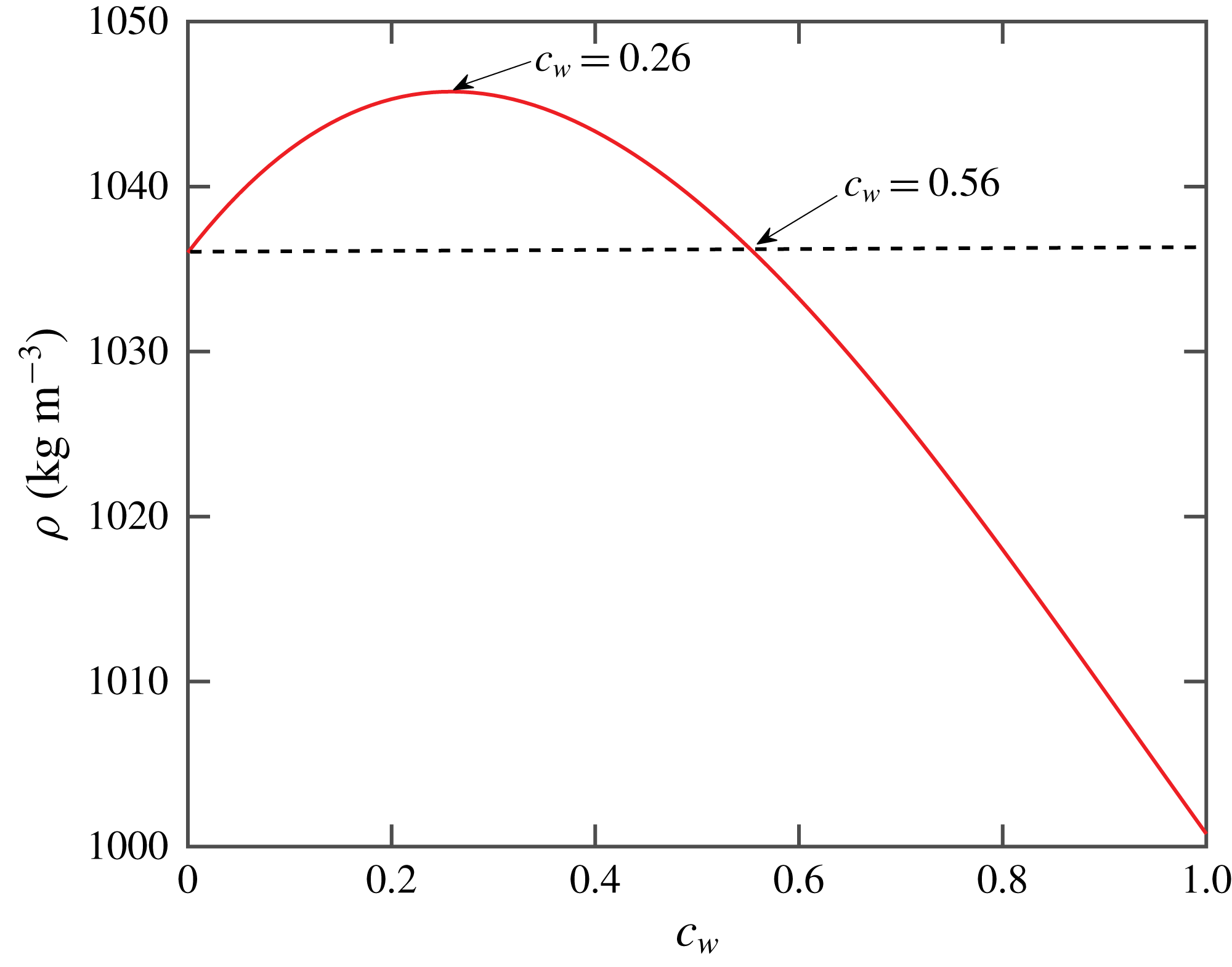
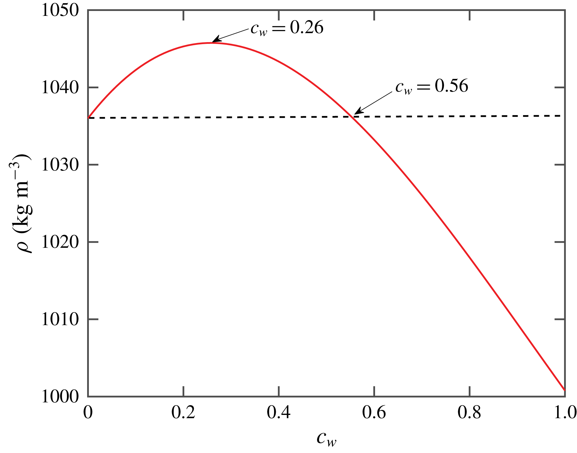
Density of water–PPG mixture as a function of the volume fraction of water (
 $c_{w}$
).
Conducting a laboratory experiment of supercritical
 $\text{CO}_{2}$
and brine at an elevated pressure (100 bar) will help to preserve the physicochemical properties of these two fluids, but this type of high-pressure experiment is inherently challenging. This motivates us to use an analogous fluid system, which maintains the key physics of the dissolution convection but allows for simpler experimental protocols. In this study, water and PPG are adopted to replace
 $\text{CO}_{2}$
and brine (Backhaus et al.
Reference Backhaus, Turitsyn and Ecke2011). This combination is similar to the
 $\text{CO}_{2}$
–brine system, in which the density of the mixture can be greater than the density of either fluid alone. As shown in figure 1, the mixture density is related to the water concentration
 $c_{w}$
via an empirical equation (Hewitt Reference Hewitt2014):
 $$\begin{eqnarray}\unicode[STIX]{x1D70C}_{i}=64.232c_{w}^{3}-179.228c_{w}^{2}+79.772c_{w}+1036.0~\text{kg}~\text{m}^{-3}.\end{eqnarray}$$
The dashed line in figure 1 indicates the density of pure PPG, and it is clear that the mixture density with volume fraction of water in the range of
 $0<c_{w}<50\,\%$
is indeed larger than that of pure PPG. The density–concentration curve appears to be nonlinear and might lead to a sub-linear
 $Sh$
–
 $Ra$
relation (Szulczewski, Hesse & Juanes Reference Szulczewski, Hesse and Juanes2013; Emami-Meybodi et al.
Reference Emami-Meybodi, Hassanzadeh, Green and Ennis-King2015). But its effect on our study should be secondary, as our study intends to keep a constant Rayleigh number in order to isolate the effect of permeability distribution.
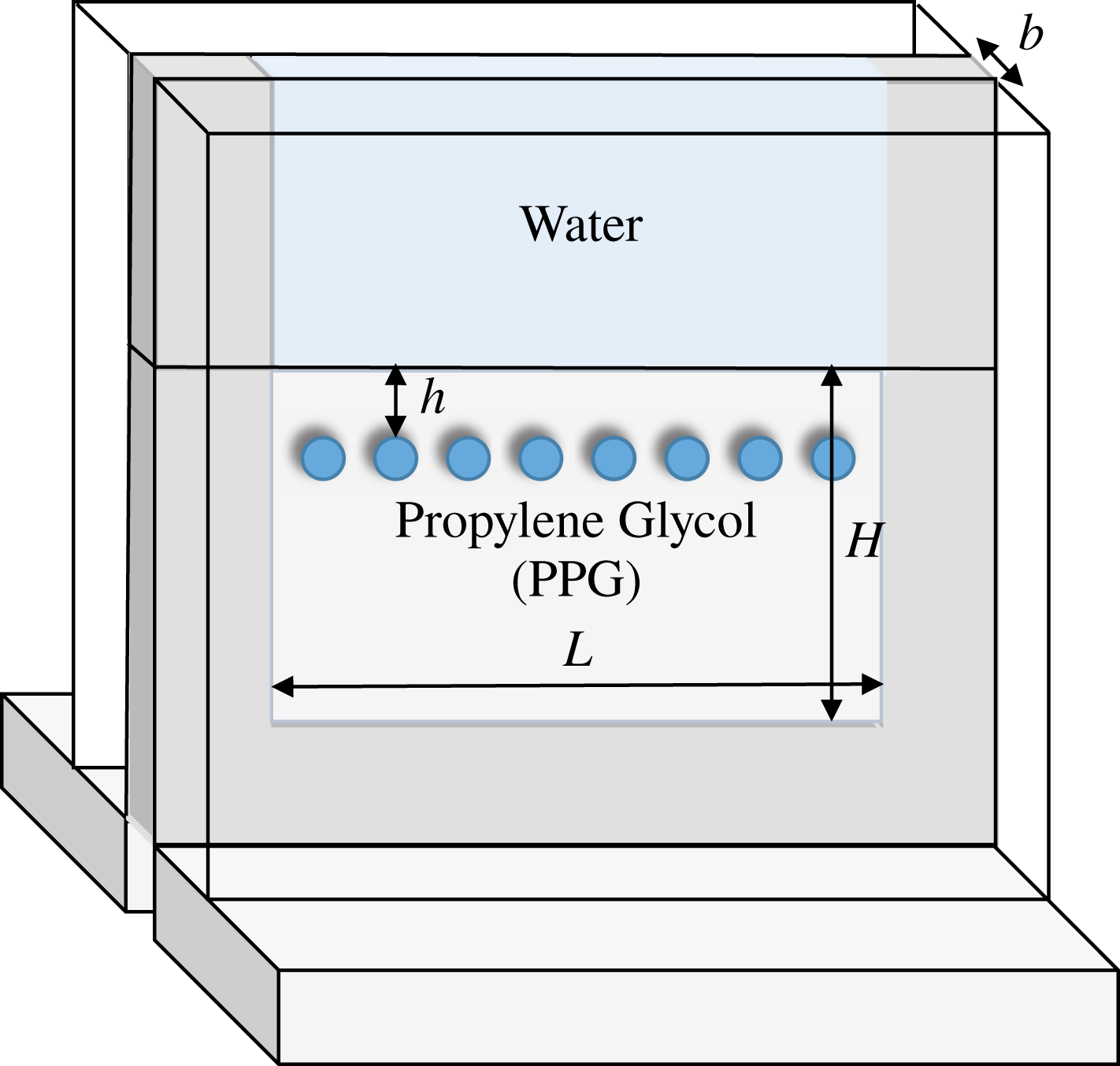
Schematic illustration of the vertical Hele-Shaw cell with a layer of discs inserted to create an environment with a heterogeneous and anisotropic permeability distribution.
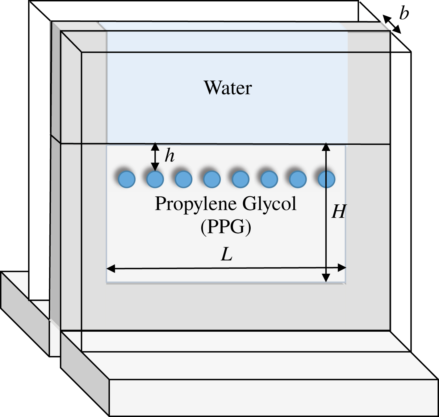
As shown in figure 2, a vertically oriented Hele-Shaw cell made of two pieces of borosilicate glass is used to make sure that the flow in this system obeys Darcy’s law. A U-shaped metal frame with a uniform thickness
 $b$
and an inner dimension of
 $76~\text{mm}\times 76~\text{mm}$
was placed between two pieces of glass to set the gap width and the boundaries for the fluids within. Two frames with
 $b=0.254$
or 0.508 mm were used to vary the permeability,
 $k=b^{2}/12$
. This type of set-up with a uniform permeability is henceforth referred to as the homogeneous configuration. A thin metal shim is used to separate water and PPG when filling the Hele-Shaw cell, and it also sets the water–PPG interface location and the height of the PPG layer
 $H$
. Two different heights,
 $H=20$
and 50 mm, were used. When the system is ready, the metal shim will be slowly pulled away to allow the two fluids to come into contact with each other and trigger the convection process (Backhaus et al.
Reference Backhaus, Turitsyn and Ecke2011).
To introduce the heterogeneous permeability across multiple length scales, circular latex discs with identical sizes were cut by a laser cutter and inserted into the Hele-Shaw cell. Discs were aligned in a horizontal layer. In this study, we used three different disc sizes,
 $D=2.5$
, 3.5 and 4.5 mm. The thickness of the discs matches the gap of the Hele-Shaw cell, thereby completely blocking flows and creating a region with zero permeability. This arrangement introduces three new length scales: disc size (
 $D$
), disc spacing (
 $l$
) and disc–interface distance (
 $h$
). It also features two different types of heterogeneity: a horizontal layer with low mean permeability extended to the whole cell width
 $L$
, and local permeability variations from zero (discs) to the background permeability
 $k$
(between discs) at a length scale
 $D$
. The dependence of the dissolution rate on
 $D$
and
 $l$
will be introduced in § 4.2.2 and its dependence on
 $h$
will be discussed in § 4.2.3.
Similar to previous work (Backhaus et al.
Reference Backhaus, Turitsyn and Ecke2011), at the interface,
 $c_{w}$
is assumed to be a constant at 0.15, with the density of the mixture
 $\unicode[STIX]{x1D70C}_{i}=1.044~\text{g}~\text{cm}^{-3}$
based on (2.1). This density is larger than that of the underlying PPG, and the density difference is
 $\unicode[STIX]{x0394}\unicode[STIX]{x1D70C}=\unicode[STIX]{x1D70C}_{i}-\unicode[STIX]{x1D70C}_{PPG}=0.009~\text{g}~\text{cm}^{-3}$
. Driven by gravity, a heavy mixture finger will descend into the PPG layer with a terminal velocity
 $v_{c}=\unicode[STIX]{x0394}\unicode[STIX]{x1D70C}gk/\unicode[STIX]{x1D70C}_{i}\unicode[STIX]{x1D708}$
. As the entire process is dominated by convection,
 $v_{c}$
is also referred to as the convective velocity. With such velocity, it takes convection approximately a time
 $t_{c}=H/v_{c}$
to travel the entire PPG layer with height
 $H$
. On the other hand, if the mass is transported solely by diffusion, it would take the mixture approximately
 $t_{d}=H^{2}/D_{m}$
to pass a distance of
 $H$
at a diffusive velocity
 $v_{d}=D_{m}/H$
, in which
 $D_{m}=10^{-6}~\text{cm}^{2}~\text{s}^{-1}$
is the mass diffusivity (Hubel, Bidault & Hammer Reference Hubel, Bidault and Hammer2002). The Rayleigh number can be calculated using the ratio between these two velocities:
 $$\begin{eqnarray}Ra=v_{c}/v_{d}=\unicode[STIX]{x0394}\unicode[STIX]{x1D70C}gHk/\unicode[STIX]{x1D70C}_{i}\unicode[STIX]{x1D708}D_{m},\end{eqnarray}$$
with
 $\unicode[STIX]{x1D708}=0.1~\text{cm}^{2}~\text{s}^{-1}$
(Rahbari-Sisakht, Taghizadeh & Eliassi Reference Rahbari-Sisakht, Taghizadeh and Eliassi2003) being the viscosity of the mixture. Both
 $D_{m}$
and
 $\unicode[STIX]{x1D708}$
are assumed to be constants in this study.
The dimensionless mass transfer rate is defined as the Sherwood number,
 $Sh={\dot{m}}/\unicode[STIX]{x1D70C}(D_{m}/H)bL$
, the ratio between the total mass flux
 ${\dot{m}}$
and the diffusive mass flux. It is challenging to directly measure the value of mass flux,
 ${\dot{m}}$
, from experiments, so it is indirectly estimated from the interfacial velocity,
 $v^{\ast }=\text{d}H^{\ast }/\text{d}t^{\ast }$
. Here
 $H^{\ast }$
is the dimensionless height of the PPG layer at each time instant. Then
 $Sh$
is formulated as the product of
 $Ra$
and the interfacial velocity:
 $$\begin{eqnarray}Sh=(\text{d}H^{\ast }/\text{d}t^{\ast })Ra,\end{eqnarray}$$
with a dimensionless time scale
 $t^{\ast }=t/t_{c}$
.
3 Experimental procedure
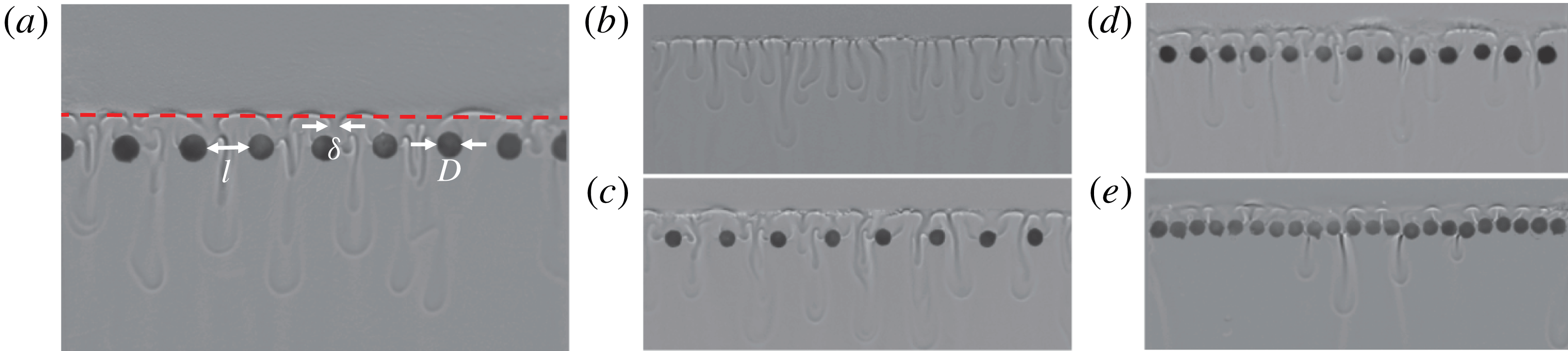
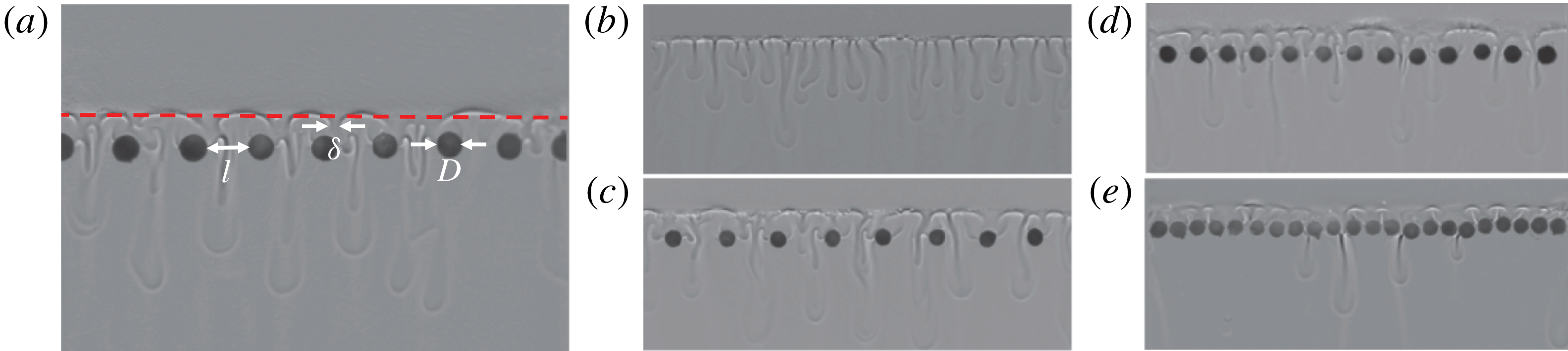
Shadowgraph images of dissolution-driven convection in a vertical Hele-Shaw cell with (a)
 $D=5.63~\text{mm}$
and
 $l=1.64~\text{mm}$
, (b) no discs, and (c–e)
 $D=2.5~\text{mm}$
and
 $l=4.8$
, 2.2 and 0.47 mm, respectively. The interface location in (a) is marked with a dashed red line that is extracted using the method introduced in § 3.
Before each experiment, all the components of the Hele-Shaw cell were cleaned and dried using compressed air to prevent contaminated surfaces from trapping small bubbles. The U-shaped metal frame was placed on the surface of one piece of glass. A layer of discs was then positioned at the designated location. After that, the other piece of glass was clamped on, and the edge of the frame was sealed with vacuum grease to complete the set-up. The entire cell was then oriented vertically so that it could be filled with fluids. PPG was injected slowly into the cell until it reached the level of a metal shim; the shim was used to separate the two fluids and any excess PPG above the shim was removed using a dry tissue. Finally water was injected following the same procedure, and the set-up was ready. The camera began to record when the shim was slowly pulled away to start an experiment.
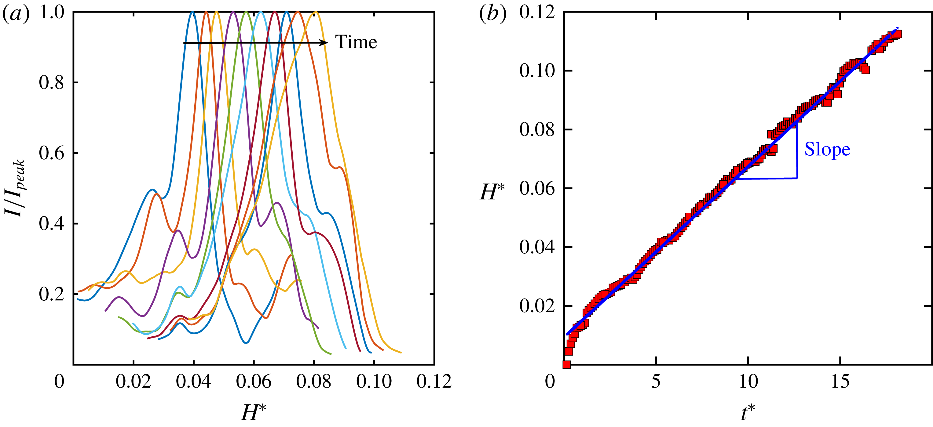
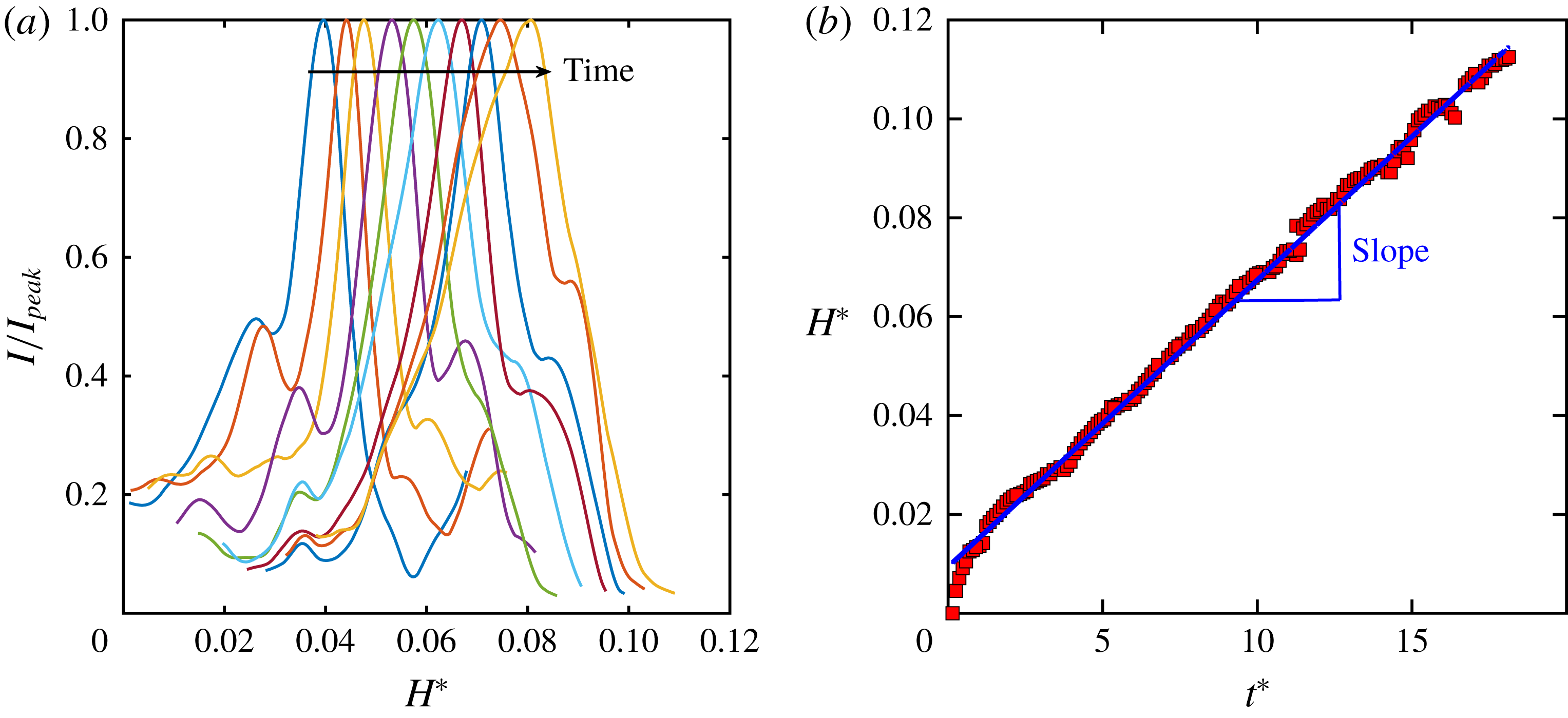
Light is generated from a fibre optic light source and condensed through a Fresnel lens. The shadow of the flow structures was projected onto a Mylar sheet and recorded by a camera at two frames per minute over seven hours. Raw images were processed to remove background. The results are shown in figure 3(a–e), and interface and fingers are clearly visible. The interface appears to be a straight line extended horizontally with a strong contrast for all disc configurations, from no discs (b) to discs with tight spacing (e). The vertical intensity profiles for one configuration (figure 3(a)) at different times are shown in figure 4(a). This profile is acquired directly from the shadowgraph image by averaging vertical lines of pixels in the entire image along the horizontal direction. The interface location can be determined from the peak of the intensity profile. To validate this method, the interface position from this method is shown in figure 3(a) as a dashed red line, which clearly overlaps with the interface. The interface moves as a function of time, and their relationship appears to be linear for a long time, as shown in figure 4(b). The blue solid line in figure 4(b) indicates a linear fit, which collapses perfectly with the data points. This linear relationship implies that a constant-flux regime exists even for a heterogeneous porous medium. The slope of this linear curve was used to calculate the mass transfer rate (
 $\text{d}H^{\ast }/\text{d}t^{\ast }$
) and the Sherwood number,
 $Sh=(\text{d}H^{\ast }/\text{d}t^{\ast })Ra$
.
(a) Normalized intensity profile across the interface at different time steps extracted from shadowgraph images (figure 3
a). (b) Extracted peak positions from (a) versus the normalized time
 $t^{\ast }=t/t_{c}$
. The solid blue line shows a linear fit to the symbols.
4 Experimental results
4.1 A homogeneous medium
The baseline experiments to validate our experimental procedure are to measure the
 $Sh$
–
 $Ra$
relationship in a homogeneous medium with no discs. The
 $Ra$
value is chosen to be around
 $10^{4}$
(Neufeld et al.
Reference Neufeld, Hesse, Riaz, Hallworth, Tchelepi and Huppert2010). Two different heights,
 $H=20$
and 50 mm, and two different gap widths,
 $b=0.254$
and 0.508 mm, were used to cover a range of
 $Ra=10^{4}{-}10^{5}$
. The
 $Sh$
–
 $Ra$
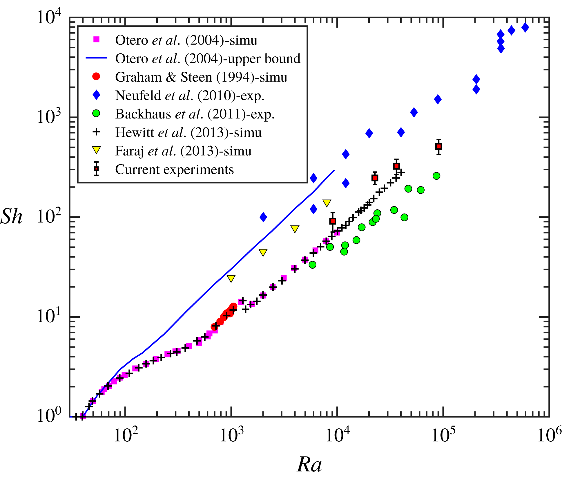
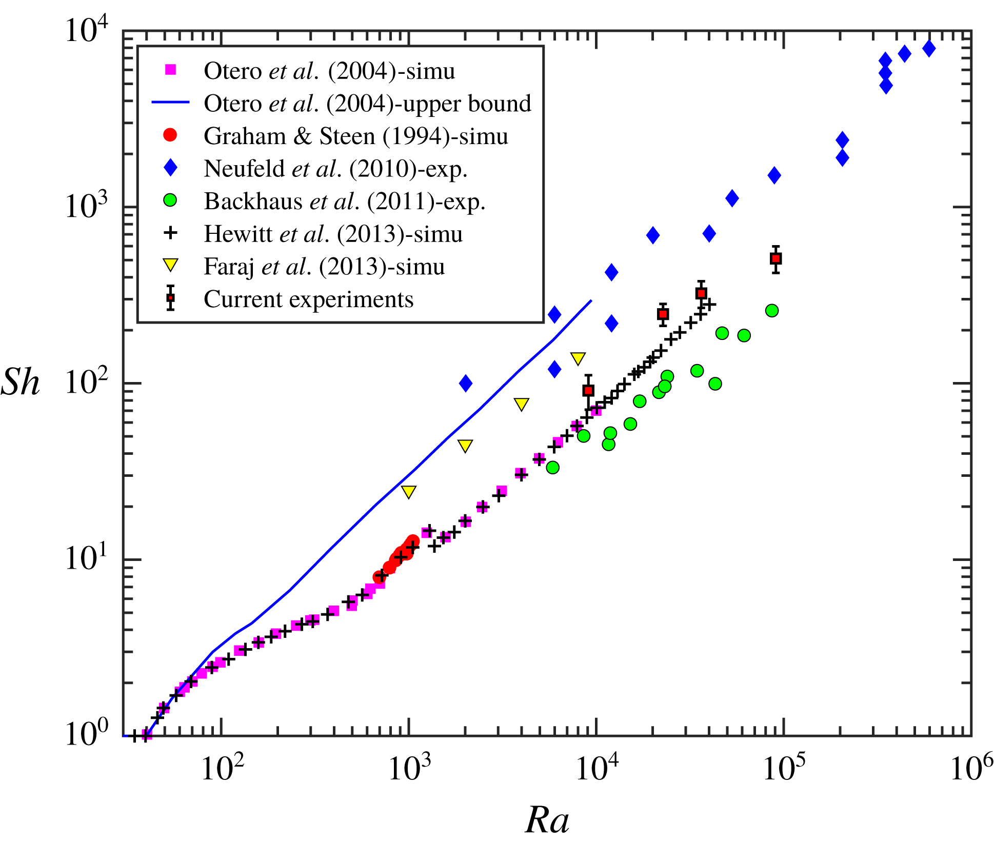
relationships obtained from our experiments were compared with several previous datasets as shown in figure 5. Both the degree of data scatter and the scaling exponent of
 $Sh$
–
 $Ra$
in our experiments are very close to those of a previous experiment in a similar configuration (Backhaus et al.
Reference Backhaus, Turitsyn and Ecke2011), but
 $Sh$
from our experiments are systematically higher. To rule out the possibility of contaminated fluid or batch difference, propylene glycol purchased from different vendors (Essential Depot, Dow Chemicals) and different types of water, including tap water and distilled water, were used. It turns out that using tap water will lead to approximately 11 % overestimation of the mass dissolution rate. But as long as distilled water is used, the reproducibility of our experiment remains in the 6.5 % range, including two different types of PPG that we used. In sum, this uncertainty due to fluid contamination or batch difference cannot explain the systematic shift between our dataset and the previous work (Backhaus et al.
Reference Backhaus, Turitsyn and Ecke2011). Although our
 $Sh$
are larger, they are still within the range bounded by two different experiments by Neufeld et al. (Reference Neufeld, Hesse, Riaz, Hallworth, Tchelepi and Huppert2010) and Backhaus et al. (Reference Backhaus, Turitsyn and Ecke2011), and our results appear to be closer to simulation results from Otero et al. (Reference Otero, Dontcheva, Johnston, Worthing, Kurganov, Petrova and Doering2004). Although the focus of this study is not on the Rayleigh-number dependence, these measurements mark the baseline of dissolution-driven convective mass transfer in a homogeneous medium.
Compilation of
 $Sh$
–
 $Ra$
in a homogeneous porous medium from previous simulations and experiments, together with a few data points from the current work.
4.2 A heterogeneous medium
4.2.1 The Sherwood number
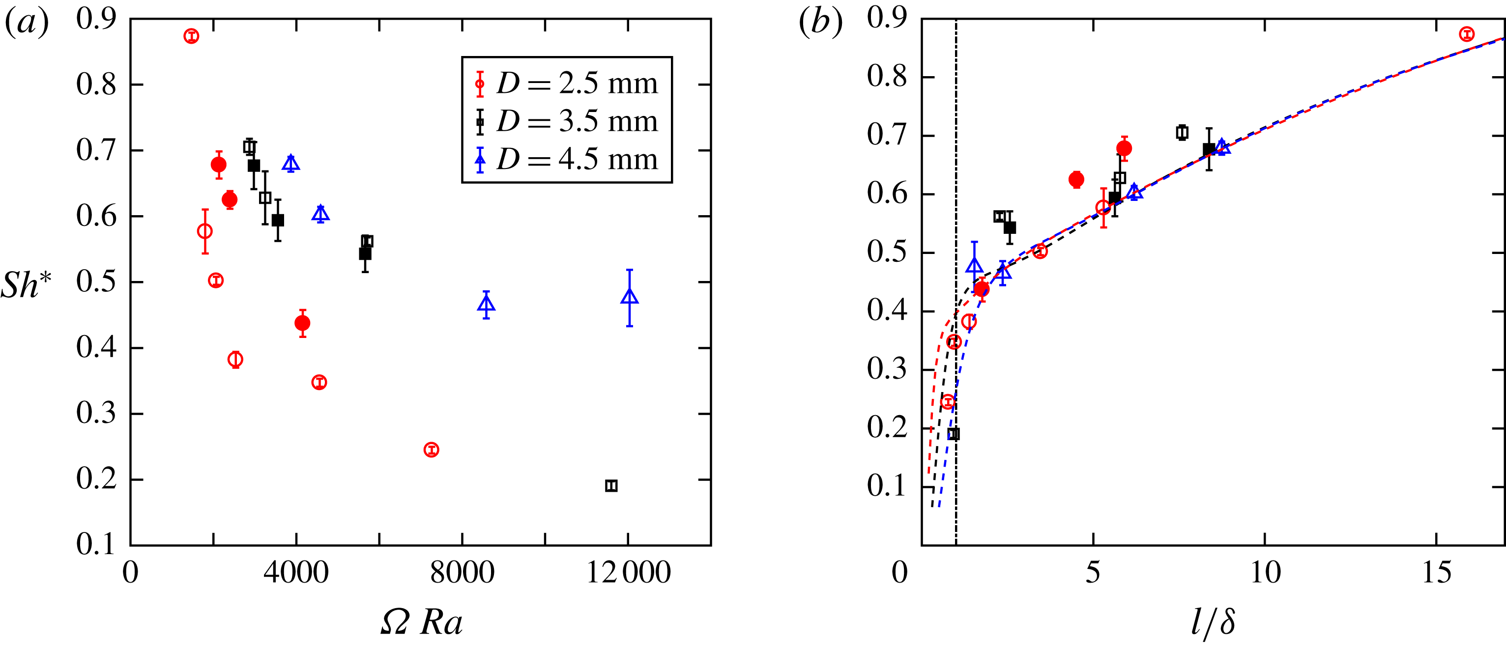
(a) Normalized Sherwood number
 $Sh^{\ast }$
as a function of
 $\unicode[STIX]{x1D6FA}\,Ra$
for various disc sizes at
 $Ra=9.87\times 10^{3}$
(solid markers) and
 $2.27\times 10^{4}$
(open markers). (b) Plot of
 $Sh^{\ast }$
versus normalized disc spacing
 $l/\unicode[STIX]{x1D6FF}$
. The vertical dash-dotted line marks
 $l/\unicode[STIX]{x1D6FF}=1$
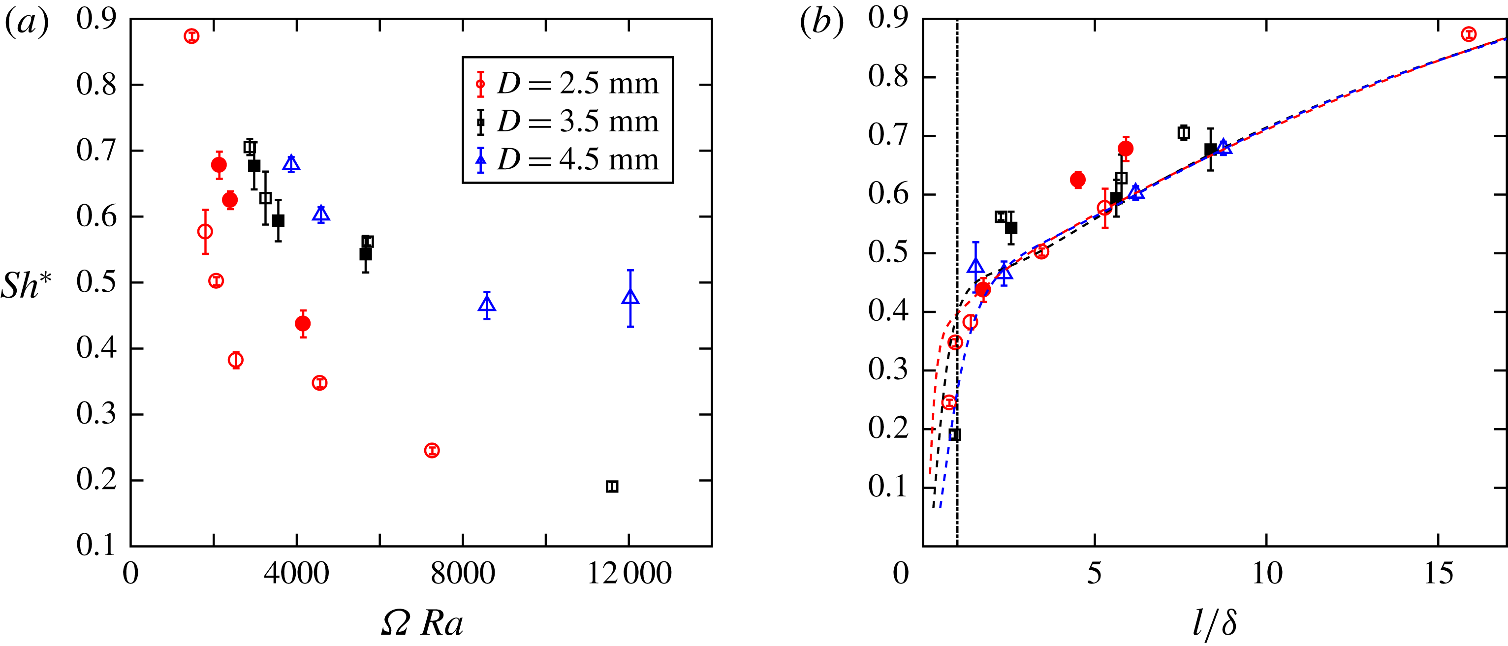
. The dashed lines show our model predictions (for details, see § 4.2.2).
Adding a layer of impermeable discs will reduce the permeability. The disc layer permeability
 $k_{l}$
is quantified using simulations (for details, see Appendix), and it is found that
 $k_{l}/k\approx l/(l+D)$
, where
 $k$
represents the permeability of the rest of the cell with no discs. Since the disc layer represents only a small portion of the PPG layer, the addition of such a layer affects the mean bulk permeability by less than 10 %. This will translate to
 ${\sim}10\,\%$
change of the Rayleigh number, which is small enough that it does not affect the
 $Sh$
significantly. In a previous work (Hewitt et al.
Reference Hewitt, Neufeld and Lister2014), the dimensionless impedance,
 $\unicode[STIX]{x1D6FA}=(D/H)/(k_{l}/k)$
, was defined to quantify the addition of a low-permeability layer. The same method is adopted here to test if the mean permeability of the disc layer is the controlling parameter.
To help with the discussion, the Sherwood number from a heterogeneous medium,
 $Sh_{het}$
, was normalized by its homogeneous counterpart,
 $Sh_{hom}$
, i.e.
 $Sh^{\ast }=Sh_{het}/Sh_{hom}$
, which ranges from zero to one. Two different heights
 $H$
of the PPG layer allow us to have two different Rayleigh numbers,
 $Ra=9.87\times 10^{3}$
and
 $Ra=2.27\times 10^{4}$
. Figure 6(a) shows
 $Sh^{\ast }$
as a function of
 $\unicode[STIX]{x1D6FA}\,Ra$
. In addition to
 $\unicode[STIX]{x1D6FA}$
,
 $Ra$
is added to compensate for the systematic shift of datasets from two different Rayleigh numbers (open and closed symbols). Although
 $\unicode[STIX]{x1D6FA}$
helps to collapse all datasets in a simulation (Hewitt et al.
Reference Hewitt, Neufeld and Lister2014), it does not work for our experiments with different disc configurations, as shown in figure 6(a). Note that there are two features of our experimental configuration that differ from the numerical set-up: (a) the simulation is on two-sided thermal convection, whereas our experiment focuses on one-sided dissolution-driven convection; and (b) the permeability within the inserted layer in the numerical configuration is uniform, whereas our low-permeability layer consists of alternating low- and high-permeability zones.
The dimensionless impedance
 $\unicode[STIX]{x1D6FA}$
is a function of two new length scales,
 $D$
and
 $l$
. Since
 $\unicode[STIX]{x1D6FA}$
does not work, we decided to take a step back and study the dependence of
 $Sh$
on either
 $D$
or
 $l$
alone. Figure 6(b) shows
 $Sh$
as a function of
 $l$
. In figure 6(b),
 $l$
is normalized by a constant
 $\unicode[STIX]{x1D6FF}$
, which represents the width of mixture fingers developed from the interface;
 $\unicode[STIX]{x1D6FF}$
is measured directly from the shadowgraph images by extracting the width of a finger at around 0.6–0.7 mm away from the interface. Even though the finger width will continue to grow as fingers descend, we chose to quantify the finger width at this fixed location because it is where the fingers have the best contrast and the smallest width. The same measurements of
 $\unicode[STIX]{x1D6FF}$
were repeated in all disc configurations, and
 $\unicode[STIX]{x1D6FF}$
is found to be a constant at 0.63 mm in all disc configurations. In figure 6(b), a collapse of all data points suggests that
 $l/\unicode[STIX]{x1D6FF}$
might be a better parameter to characterize the heterogeneity for our configuration. These data points share one trend:
 $Sh^{\ast }$
decreases with decreasing
 $l$
, and it drops sharply at
 $l/\unicode[STIX]{x1D6FF}\approx 1$
. This is because
 $l/\unicode[STIX]{x1D6FF}$
characterizes two different flow regimes: convective fingers freely pass through the gap for
 $l/\unicode[STIX]{x1D6FF}>1$
, and no finger directly passes through the gap for
 $l/\unicode[STIX]{x1D6FF}<1$
. The surprising part is that the results show weak dependence, if at all, on
 $D$
, at least in the range of
 $D$
that we used. Note that
 $D$
represents the distance between two high-permeability channels as well as the thickness of the disc layer. This finding may have important implications to subsurface carbon sequestration. For example, if the geological formation has some low-permeability layers filled with fractures (high-permeability gaps), it is possible that the fracture width is the dominant factor that controls the convective flow, and fracture–fracture distance and layer thickness are secondary.
4.2.2 Model
Convective mass transfer is primarily conducted by descending mixture fingers. Based on this argument, the convective mass transfer rate
 ${\dot{m}}$
can be expressed as a function of the number
 $n_{f}$
, width
 $\unicode[STIX]{x1D6FF}$
, thickness
 $b$
, velocity
 $u_{f}$
and density
 $\unicode[STIX]{x1D70C}$
of these fingers,
 ${\dot{m}}=\unicode[STIX]{x1D70C}bc_{w}u_{f}n_{f}\unicode[STIX]{x1D6FF}$
. Combined with the definitions of
 $Sh$
and
 $Ra$
, it is found that
 $Sh=c_{w}n_{f}(\unicode[STIX]{x1D6FF}/L)(u_{f}/u_{c})Ra$
, which depends primarily on the volume fraction of fingers in the PPG layer,
 $n_{f}\unicode[STIX]{x1D6FF}/L$
, and the dimensionless finger velocity,
 $u_{f}/u_{c}$
(Backhaus et al.
Reference Backhaus, Turitsyn and Ecke2011).
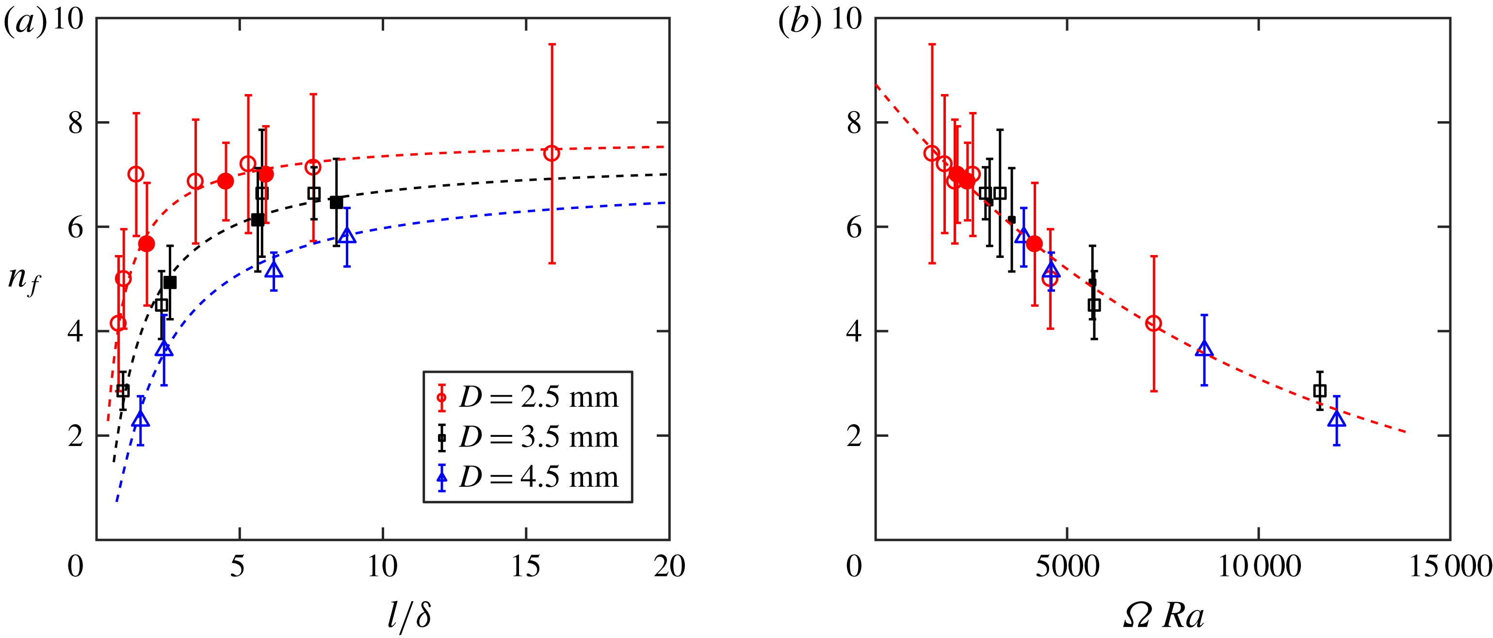
(a) Number of fingers (
 $n_{f}$
) versus normalized disc spacing
 $l/\unicode[STIX]{x1D6FF}$
at
 $Ra=9.87\times 10^{3}$
(solid markers) and
 $2.27\times 10^{4}$
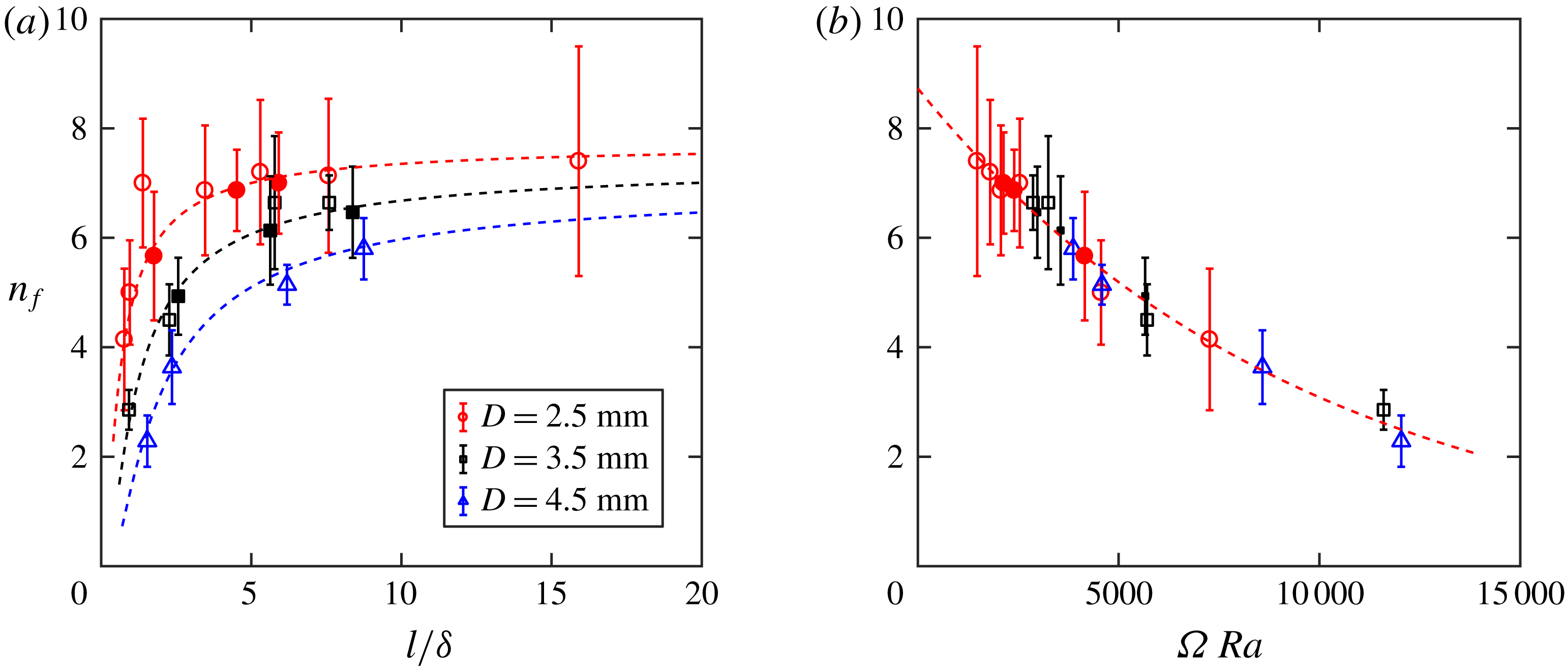
(open markers). The three dashed lines correspond to the single dashed line in (b). (b) Plot of
 $n_{f}$
versus
 $\unicode[STIX]{x1D6FA}\,Ra$
for the same datasets. The dashed line represents an exponential fit over all data points.
In
 $n_{f}\unicode[STIX]{x1D6FF}/L$
,
 $n_{f}$
represents the number of fingers that pass through the disc layer. Since
 $\unicode[STIX]{x1D6FF}/L$
is a constant, the entire term is controlled by
 $n_{f}$
. This number can be directly extracted from shadowgraph images by counting the number of fingers right below the disc layer. From these images shown in figure 3(b–e), it is obvious that
 $n_{f}$
increases as
 $l$
becomes larger, consistent with what one would expect. Figure 7(a) shows
 $n_{f}$
as a function of
 $l/\unicode[STIX]{x1D6FF}$
for different disc sizes, and the error bar indicates the variation of
 $n_{f}$
for each configuration. To our surprise,
 $l/\unicode[STIX]{x1D6FF}$
does not work to collapse all datasets for
 $n_{f}$
, even though
 $l/\unicode[STIX]{x1D6FF}$
was proven to be the parameter to quantify the heterogeneity effect for
 $Sh$
.
More surprisingly, the impedance
 $\unicode[STIX]{x1D6FA}\,Ra$
, which failed for
 $Sh$
, perfectly explains the dependence of
 $n_{f}$
, as shown in figure 7(b). The dashed line in figure 7(b) shows an exponential fit of all data points:
 $n_{f}=a\exp (-b\unicode[STIX]{x1D6FA}\,Ra)$
, in which
 $a=8.73$
and
 $b=1.04\times 10^{-5}$
. This function bridges two known limits at
 $\unicode[STIX]{x1D6FA}=0$
(no discs with zero gaps) and
 $\unicode[STIX]{x1D6FA}=\infty$
(touching discs with zero gaps). At
 $\unicode[STIX]{x1D6FA}=0$
,
 $n_{f}$
is equal to 8.73, a number that is consistent with the one obtained in a homogeneous medium (Backhaus et al.
Reference Backhaus, Turitsyn and Ecke2011). When
 $\unicode[STIX]{x1D6FA}$
approaches infinity, the layer is completely closed, and no fingers can pass, i.e.
 $n_{f}=0$
. This nice collapse of all data points onto one curve implies that
 $n_{f}$
is controlled primarily by the permeability (or impedance), rather than by the disc spacing
 $l$
.
Convective mass transfer is also affected by the finger velocity
 $u_{f}$
. Fingers moving downwards at a speed of
 $u_{f}$
will drive pure PPG between fingers to move upwards at a speed of
 $u_{b}$
. The values of
 $u_{f}$
and
 $u_{b}$
are related to the number of fingers
 $u_{f}\unicode[STIX]{x1D6FF}=(L/n_{f}-\unicode[STIX]{x1D6FF})u_{b}$
, where
 $L/n_{f}$
represents the average finger spacing. They are also related to the convective velocity
 $u_{c}$
through a path integration of Darcy’s law through a finger and a back-flow:
 $u_{c}=u_{f}+(\unicode[STIX]{x1D708}_{PPG}/\unicode[STIX]{x1D708}_{w})u_{b}$
. This will eventually lead to a new equation,
 $u_{f}/u_{c}=1/[1+(\unicode[STIX]{x1D708}_{PPG}/\unicode[STIX]{x1D708}_{w})(n_{f}\unicode[STIX]{x1D6FF}/L)/(1-(n_{f}\unicode[STIX]{x1D6FF}/L))]$
, directly linking
 $u_{f}/u_{c}$
to
 $n_{f}$
(Backhaus et al.
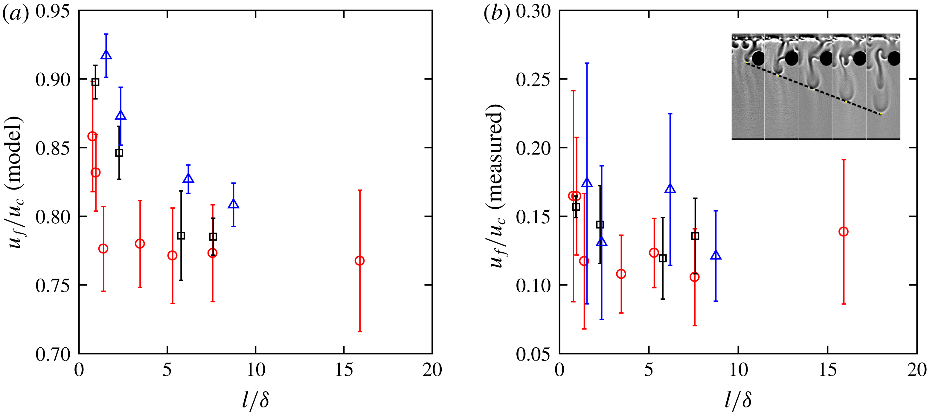
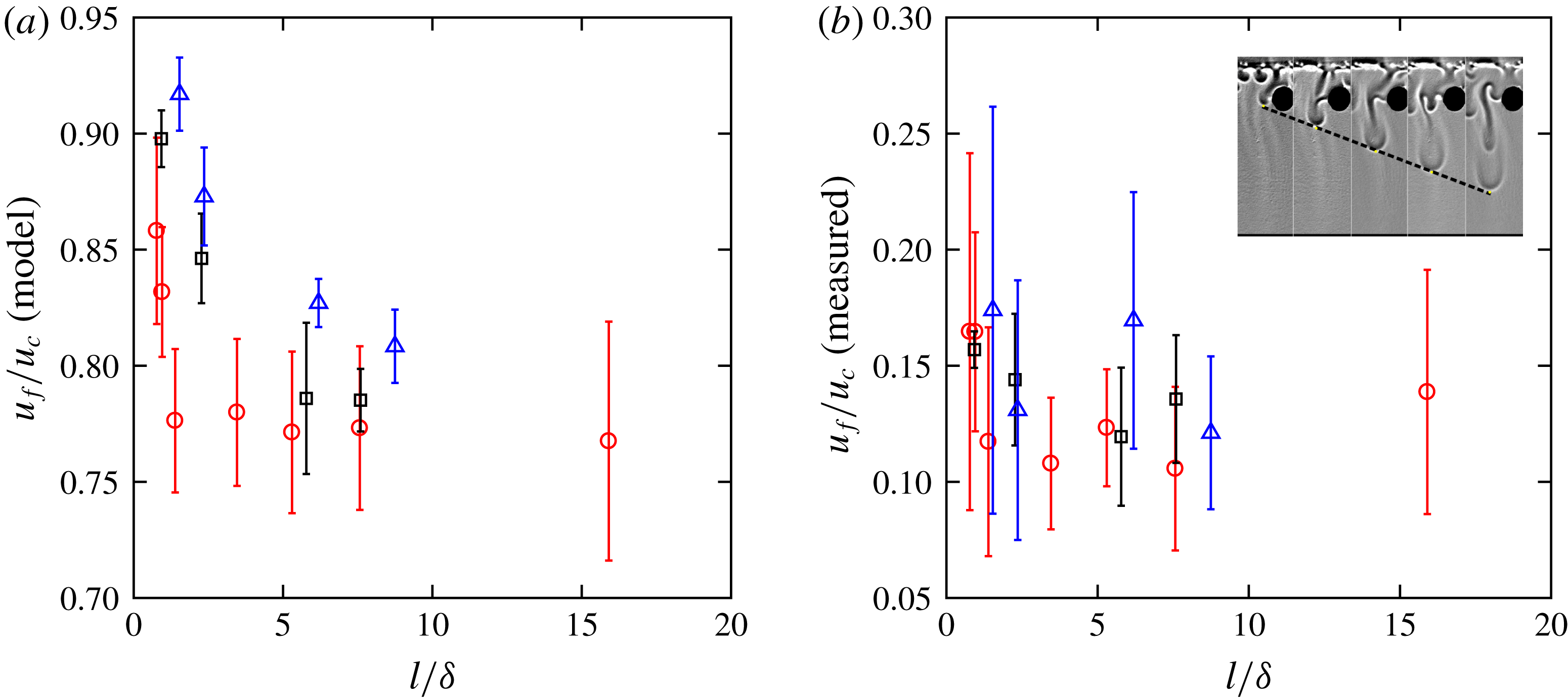
Reference Backhaus, Turitsyn and Ecke2011). As shown in figure 8(a), the calculated
 $u_{f}/u_{c}$
shows a weak dependence on
 $l/\unicode[STIX]{x1D6FF}$
. To confirm the result, an independent method from image analysis can be used to directly extract the velocity of fingers
 $u_{f}$
(Ecke & Backhaus Reference Ecke and Backhaus2016). The vertical finger velocity is determined from a sequence of images, as shown in the inset of figure 8(b). The results of measured
 $u_{f}$
normalized by
 $u_{c}$
, assuming a constant density contrast, are shown in figure 8(b). Similar to a previous work (Ecke & Backhaus Reference Ecke and Backhaus2016), the variations of finger velocity, indicated by the error bars, are large, and it is difficult to draw a conclusion about the dependence of
 $u_{f}$
on
 $l/\unicode[STIX]{x1D6FF}$
or
 $\unicode[STIX]{x1D6FA}\,Ra$
with these uncertainties. If there is any trend at all, both methods confirm that the normalized finger velocity
 $u_{f}/u_{c}$
does not change much over different disc configurations.
(a) Normalized finger velocity
 $u_{f}/u_{c}$
calculated based on the number of fingers
 $n_{f}$
and the incompressible flow condition (symbols represent different disc size
 $D$
used in figure 7), and (b)
 $u_{f}$
measured from a sequence of shadowgraph images as shown in the inset.
The analyses so far raise an important issue: if
 $Sh=c_{w}n_{f}(\unicode[STIX]{x1D6FF}/L)(u_{f}/u_{c})Ra$
holds,
 $n_{f}$
is a function of
 $\unicode[STIX]{x1D6FA}$
, and
 $c_{w}$
,
 $u_{f}/u_{c}$
and
 $Ra$
are all (close to) constants, then
 $Sh$
should also depend on
 $\unicode[STIX]{x1D6FA}$
, which is inconsistent with our findings that
 $Sh$
depends on
 $l/\unicode[STIX]{x1D6FF}$
rather than on
 $\unicode[STIX]{x1D6FA}$
. This suggests that one parameter that was assumed to be constant may exhibit a strong dependence on the disc configuration, and that parameter turns out to be the density contrast
 $\unicode[STIX]{x0394}\unicode[STIX]{x1D70C}$
in
 $Ra$
. In a homogeneous case with water above PPG,
 $\unicode[STIX]{x0394}\unicode[STIX]{x1D70C}$
represents the density difference between the mixture at the interface with PPG. The addition of the disc layer separates the system into three layers, water, upper PPG layer above discs, and lower PPG layer below discs. If encountering discs, fingers have to turn around and mix with the rest of the upper PPG layer, effectively increasing the density of the upper PPG layer. Fingers going through the upper PPG layer will therefore experience smaller density contrast with the surrounding mixture.
For this reason, we define a new parameter – the effective Rayleigh number
 $Ra_{eff}$
– to evaluate the change of the density contrast
 $\unicode[STIX]{x1D6FF}\unicode[STIX]{x1D70C}=\unicode[STIX]{x1D70C}_{in}-\unicode[STIX]{x1D70C}_{out}$
between the liquids inside (
 $\unicode[STIX]{x1D70C}_{in}$
) and outside (
 $\unicode[STIX]{x1D70C}_{out}$
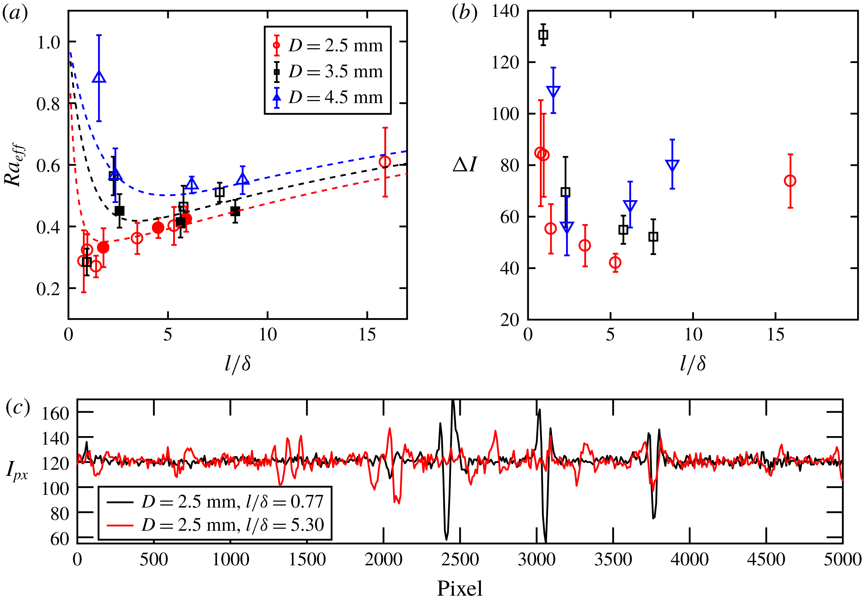
) of a finger. Figure 9(a) shows the calculated
 $Ra_{eff}=Sh/[c_{w}n_{f}(\unicode[STIX]{x1D6FF}/L)(u_{f}/u_{c})]$
as a function of
 $l/\unicode[STIX]{x1D6FF}$
. The results are normalized by
 $Ra$
using the maximum density difference
 $\unicode[STIX]{x0394}\unicode[STIX]{x1D70C}$
, so it should range from zero to one. An independent method is required to confirm that this calculated result indeed represents the finger density contrast
 $\unicode[STIX]{x1D6FF}\unicode[STIX]{x1D70C}$
. In this study,
 $\unicode[STIX]{x1D6FF}\unicode[STIX]{x1D70C}$
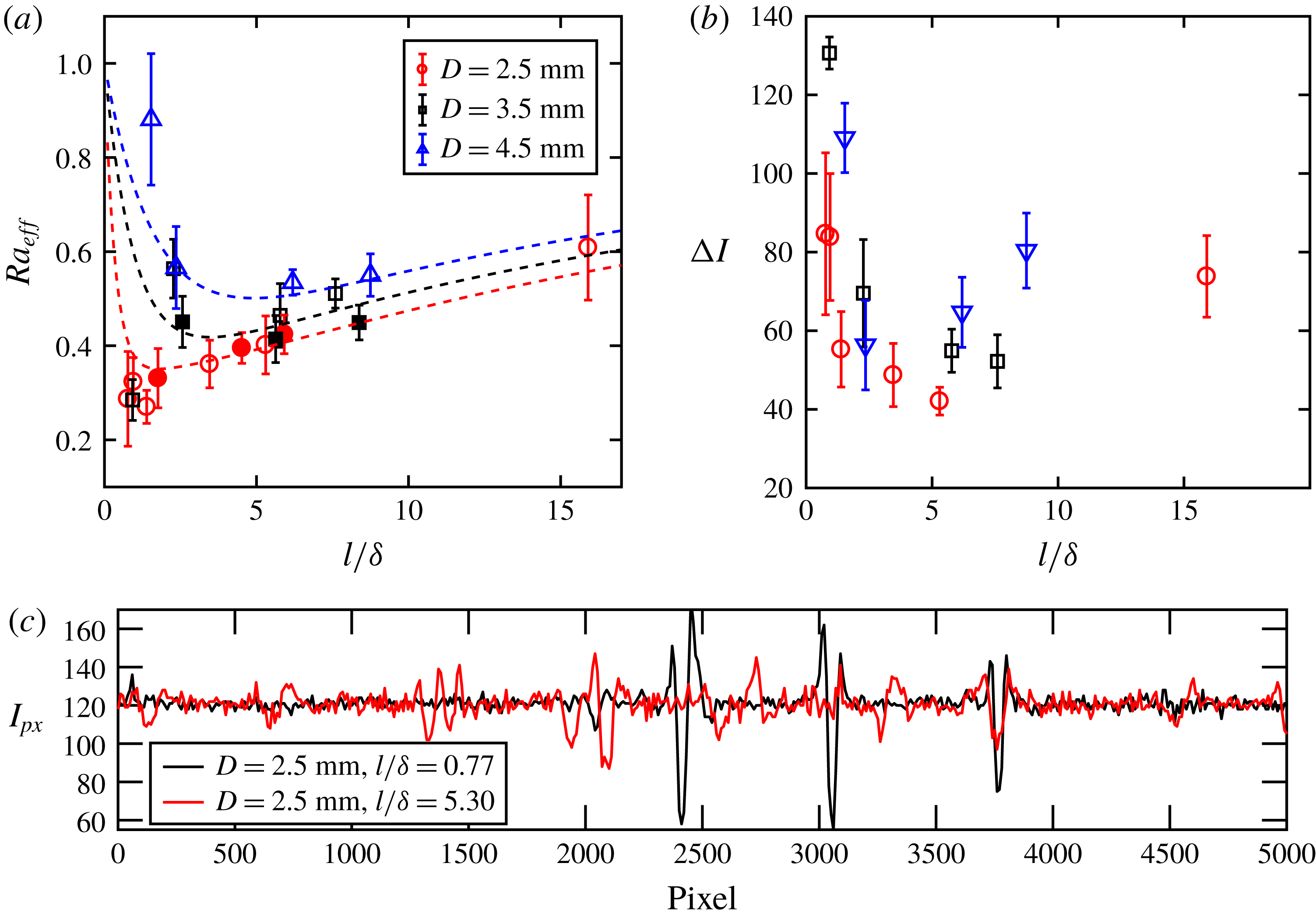
is also indirectly inferred from the intensity contrast of a finger in a shadowgraph image (MacBeth & Thompson Reference MacBeth and Thompson1951). As shown in figure 9(c), the intensity of a horizontal line of pixels right below the disc layer is obtained from shadowgraph images. Each finger can be identified by its feature as two peaks with a valley in between (Settles Reference Settles2012). The intensity difference between the peak and valley defines the intensity contrast
 $\unicode[STIX]{x0394}I$
, which provides a way to evaluate the density contrast indirectly. In figure 9(c), two intensity profiles from two experiments with the same disc size
 $D=2.5~\text{mm}$
but different
 $l/\unicode[STIX]{x1D6FF}$
(0.77 and 5.30) are shown. It is clear that, even though there are more fingers for
 $l/\unicode[STIX]{x1D6FF}=5.30$
, the
 $\unicode[STIX]{x0394}I$
of these fingers are not as strong as those for
 $l/\unicode[STIX]{x1D6FF}=0.77$
.
Figure 9(b) shows the variations of
 $\unicode[STIX]{x0394}I$
as a function of
 $l/\unicode[STIX]{x1D6FF}$
. The trend appears to be similar to that of
 $Ra_{eff}$
shown in figure 9(a). Both
 $Ra_{eff}$
and
 $\unicode[STIX]{x0394}I$
have non-monotonic dependences on
 $l/\unicode[STIX]{x1D6FF}$
, and there is a transition near
 $l/\unicode[STIX]{x1D6FF}=1\sim 3$
. These similarities imply that the trend of the calculated
 $Ra_{eff}$
can indeed characterize the density gradient of a finger in different configurations.
This finding raises more questions as to why the density contrast of fingers experiences a transition that depends on the disc spacing
 $l$
. As suggested before, this is primarily because the disc spacing controls the mixing in the upper PPG layer.
When
 $l/\unicode[STIX]{x1D6FF}\gg 1$
, most fingers from the water–PPG interface can directly pass through the disc layer. The density contrast of these fingers recovers that of the homogeneous case:
 $\unicode[STIX]{x1D6FF}\unicode[STIX]{x1D70C}=\unicode[STIX]{x1D6E5}\unicode[STIX]{x1D70C}$
. When the number of discs increases and
 $l$
decreases, some fingers start to hit discs and are forced to return and mix with the remaining PPG in the upper PPG layer. This forced mixing will effectively increase the density of the background fluid for other fingers and reduces the finger density contrast. Based on this, we argue that
 $\unicode[STIX]{x1D6FF}\unicode[STIX]{x1D70C}$
is inversely proportional to the probability of a finger encountering a disc. This probability is related to the number of discs
 $N_{D}=L/(l+D)$
. In addition, the functional form linking
 $\unicode[STIX]{x1D6FF}\unicode[STIX]{x1D70C}$
and
 $N_{D}$
has to satisfy two limiting cases for
 $l=0$
and
 $l=L$
. So we choose
 $\unicode[STIX]{x1D6FF}\unicode[STIX]{x1D70C}=c_{2}\exp (-\unicode[STIX]{x1D6FD}N_{D})$
, which is bounded when
 $N_{D}$
approaches zero or infinity.
For the other regime, when
 $l/\unicode[STIX]{x1D6FF}<1$
, the probability of a finger encountering a disc is no longer relevant to
 $\unicode[STIX]{x1D6FF}\unicode[STIX]{x1D70C}$
. For such a tight constraint, no fingers from the interface can cross the disc layer directly; all of them have to mix in the upper PPG layer and wait until the density of this layer becomes high enough to push some new fingers through those tight constraints. That explains why
 $\unicode[STIX]{x1D6FF}\unicode[STIX]{x1D70C}$
increases with decreasing
 $l/\unicode[STIX]{x1D6FF}$
, as tighter constraints will require a higher density contrast to push the mixture through. To achieve bounded values at two limiting cases, we again model
 $\unicode[STIX]{x1D6FF}\unicode[STIX]{x1D70C}=c_{1}\exp (-\unicode[STIX]{x1D6FC}l/\unicode[STIX]{x1D6FF})$
.
(a) The effective Rayleigh number
 $Ra_{eff}$
calculated from
 $Sh/[c_{w}n_{f}(\unicode[STIX]{x1D6FF}/L)(u_{f}/u_{c})]$
versus different disc spacings
 $l/\unicode[STIX]{x1D6FF}$
, (b) the intensity contrast
 $\unicode[STIX]{x0394}I$
of fingers extracted from the intensity profile shown in (c), and (c) the intensity profile of a horizontal line of pixels located right below the disc layer in a shadowgraph image.
The superposition of these two extreme limits helps to model the trend of
 $Ra_{eff}$
versus
 $l/\unicode[STIX]{x1D6FF}$
from
 $l/\unicode[STIX]{x1D6FF}=0$
to
 $L/\unicode[STIX]{x1D6FF}$
:
 $$\begin{eqnarray}Ra_{eff}=C_{1}\left[\exp \left(-\unicode[STIX]{x1D6FC}\frac{l}{\unicode[STIX]{x1D6FF}}\right)+C_{2}\exp \left(-\unicode[STIX]{x1D6FD}\frac{L/\unicode[STIX]{x1D6FF}}{l/\unicode[STIX]{x1D6FF}+D/\unicode[STIX]{x1D6FF}}\right)\right]+C_{3}.\end{eqnarray}$$
The second exponential term can also be written as
 $C_{2}\exp [-\unicode[STIX]{x1D6FD}(H/D)(L/l)\unicode[STIX]{x1D6FA}]$
, where
 $\unicode[STIX]{x1D6FA}=(D/H)/(k_{l}/k)$
and
 $k_{l}/k\approx l/(l+D)$
. Thus
 $Ra_{eff}$
becomes a complicated function of both
 $l/\unicode[STIX]{x1D6FF}$
and
 $\unicode[STIX]{x1D6FA}$
, so it cannot be collapsed by either one alone. This model emphasizes the importance of the disc spacing
 $l$
in controlling the mixing process and the dissolution mass transfer rate. More importantly,
 $l$
plays an opposite role in two different regimes separated by
 $l/\unicode[STIX]{x1D6FF}\approx 1$
, which is surprising but successfully captured by our model. Note that, although there are five parameters, they are not all independent:
 $C_{2}$
and
 $C_{3}$
are determined from a combination of three other parameters by imposing the conditions at two limiting cases at
 $l=0$
and
 $l=L$
. In both cases when the disc layer is completely closed at
 $l=0$
or completely open at
 $l=L$
, the finger density contrast
 $\unicode[STIX]{x1D6FF}\unicode[STIX]{x1D70C}$
should recover the largest density contrast
 $\unicode[STIX]{x0394}\unicode[STIX]{x1D70C}$
, and the normalized
 $Ra_{eff}$
goes to one.
The dashed lines in figure 9(a) show the modelled
 $Ra_{eff}$
following (4.1). Three parameters,
 $C_{1}$
,
 $\unicode[STIX]{x1D6FC}$
and
 $\unicode[STIX]{x1D6FD}$
, in the model are fitted to these data points;
 $C_{2}$
is found to be close to one. Since
 $C_{2}$
controls the relative weight of two exponential functions, it suggests that both mixing mechanisms are equally important for the intermediate range of
 $l/\unicode[STIX]{x1D6FF}\approx 1$
. For three different disc sizes,
 $\unicode[STIX]{x1D6FD}$
,
 $C_{2}$
and
 $C_{3}$
are in a similar range (0.1–1). On the other hand,
 $C_{1}$
and
 $\unicode[STIX]{x1D6FC}$
exhibit relatively stronger dependences on disc sizes, even though the values are still around the order of unity. In addition, since the two exponential terms have the opposite dependences on
 $l/\unicode[STIX]{x1D6FF}$
, once
 $l/\unicode[STIX]{x1D6FF}$
crosses from one regime to the other, one term will become dominant over the other one and control the
 $Ra_{eff}$
dependence very quickly.
Equation (4.1) can also be used to confirm the Sherwood-number dependence by multiplying
 $Ra_{eff}$
with the exponential fit of
 $n_{f}$
and functional form of
 $u_{f}/u_{c}$
derived from the incompressible flow conditions. The results are shown in figure 6(b) as dashed lines, which seem to collapse well with the experimental results and show a clear transition near
 $l/\unicode[STIX]{x1D6FF}=1$
. It is important to emphasize that, although
 $\unicode[STIX]{x1D6FF}\unicode[STIX]{x1D70C}$
tends to increase with decreasing
 $l$
when
 $l/\unicode[STIX]{x1D6FF}<1$
, the overall dissolution rate decreases sharply in this regime, because increasing
 $\unicode[STIX]{x1D6FF}\unicode[STIX]{x1D70C}$
is not sufficient to compensate for significantly fewer fingers through the disc layer.
4.2.3 Interface position
Finally, the effect of relative distance
 $h$
from the water–PPG interface to the disc layer will be discussed. For
 $h$
, there are two extreme cases,
 $h=0$
and
 $h=H$
. At
 $h=0$
, the disc layer directly touches the interface, so it becomes challenging to control and monitor the disc–interface interaction. We decided to start with
 $h=3\unicode[STIX]{x1D6FF}$
(2 mm), which is away from the interface so that the disc does not interfere with the boundary layer dynamics. All the discussions so far are based on disc configurations at this constant
 $h=3\unicode[STIX]{x1D6FF}$
. The other limit is at
 $h=H$
. For this case, the disc is at the bottom of the PPG layer, and it will contribute very little to the fingering dynamics. In order to investigate how the Sherwood number transitions from one limit to the other, we have systematically investigated the dependence of
 $Sh$
on
 $h$
.
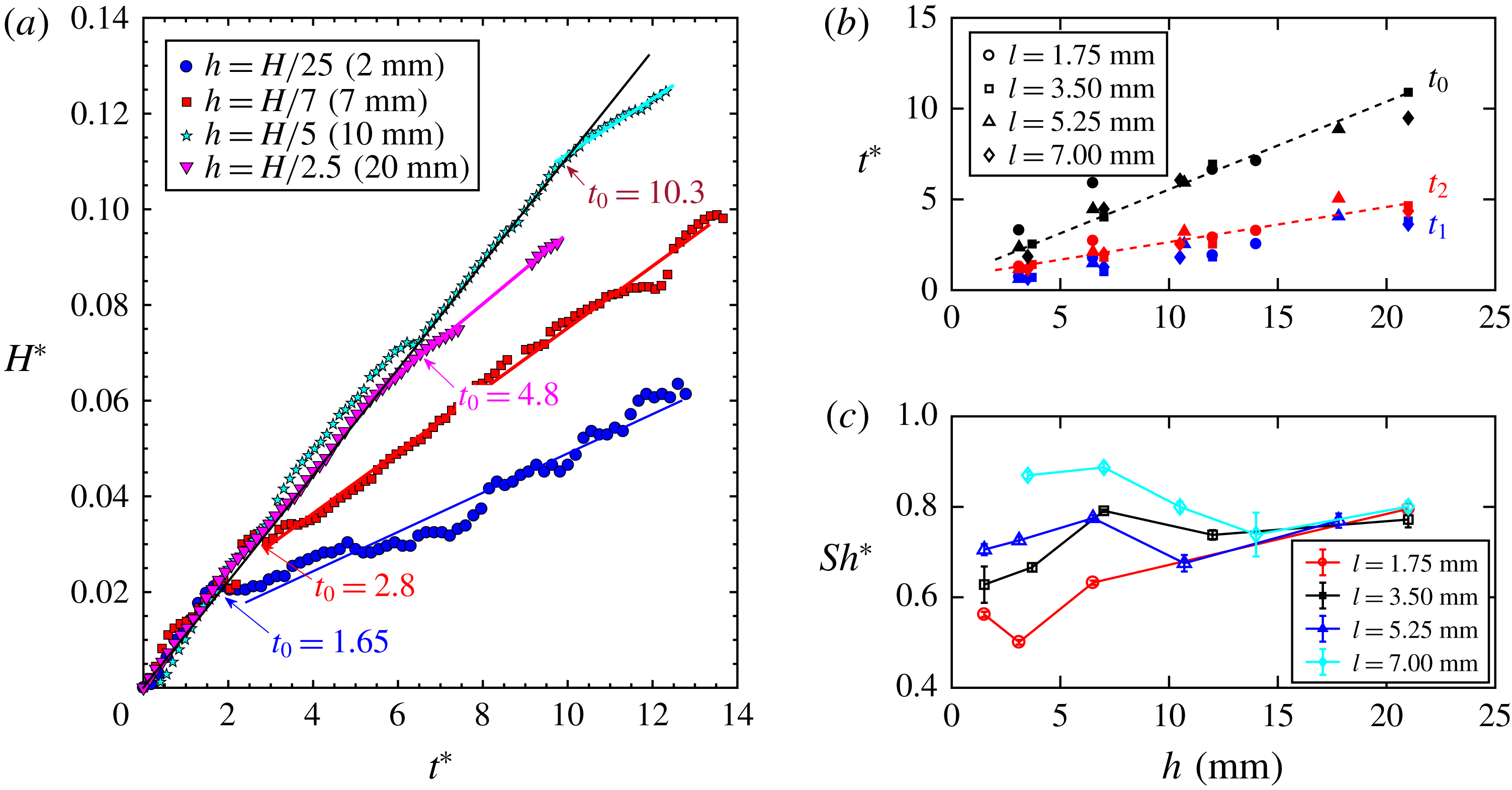
(a) The normalized interface location versus time. Arrows point at the transition time
 $t_{0}$
between two linear regimes with different slopes. (b) The transition time
 $t_{0}$
(black), as well as the time that it takes for mixture fingers travelling from the water–PPG interface to the top (
 $t_{1}$
, blue) and bottom (
 $t_{2}$
, red) of the disc layer, are shown as functions of the separation
 $h$
between the disc layer and the interface. The two dashed lines are linear fits to red and black symbols, respectively. The slopes of these two lines differ by a factor of 2.5. (c) The normalized Sherwood number as a function of
 $h$
for different disc spacings
 $l$
.
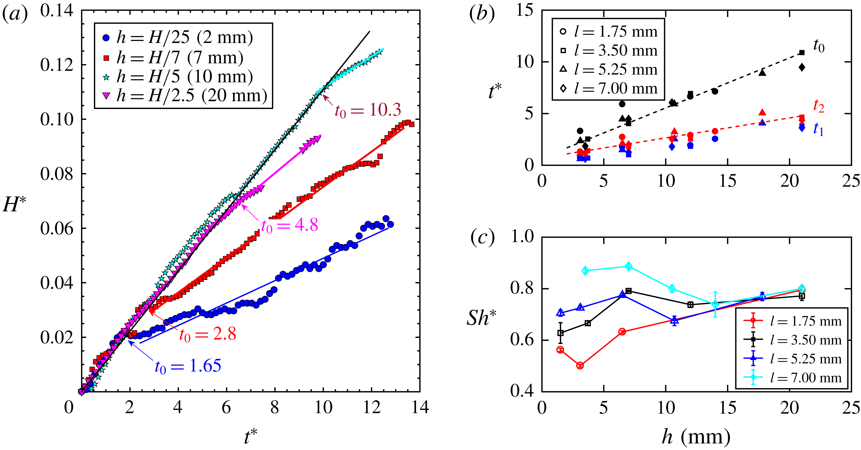
As shown in figure 10(a), the interface height rises as a function of time for four different
 $h$
values. But instead of having one linear line, all curves show a rather sharp transition from one linear regime to another. Before the transition, all curves seem to collapse onto one line, as indicated by the black solid line. The slope of this line recovers that of the homogeneous configuration with no discs, indicating that the dynamics in the very beginning tends to be the same until the system starts to sense the existence of the disc layer. After the transition, the slope drops significantly, suggesting a sudden reduction of the mass transfer rate. The transition time
 $t_{0}$
appears to increase with
 $h$
. To confirm that,
 $t_{0}$
for different
 $h$
and
 $l$
is shown in figure 10(b) (black symbols) for different disc configurations. It seems that
 $t_{0}$
increases linearly with respect to
 $h$
.
The results suggest that the presence of the disc layer will not be sensed until the first group of fingers touch the disc layer after travelling a distance
 $h$
from the interface. If the travelling speed of the fingers in all configurations stays the same, the transition time
 $t_{0}$
will increase linearly with
 $h$
. In figure 10(b), in addition to
 $t_{0}$
, the average times for fingers to travel from the interface to the top (
 $t_{1}$
, blue) and bottom (
 $t_{2}$
, red) of the disc layer are also shown. These two time delays are extracted from the shadowgraph movies. Times
 $t_{1}$
and
 $t_{2}$
are close to each other, and both of them depend linearly on
 $h$
, indicating that fingers travel indeed at a constant speed independent of
 $h$
. But the slopes of
 $t_{1}$
and
 $t_{2}$
with respect to
 $h$
are smaller than that of the transition time
 $t_{0}$
. In figure 10(b), two dashed lines show linear fits of
 $t_{0}$
and
 $t_{2}$
. The slopes of these two lines differ roughly by a factor of 2.5, i.e.
 $t_{0}=2.5t_{2}$
for all disc configurations. Note that the convective mass transfer rate is measured by detecting the interface rising velocity. Although fingers take time
 $t_{2}$
to travel to the disc layer, it might take another time
 $t_{2}$
to bring the disc layer effect back to the interface by those turn-around fingers to complete the mixing. Adding these two travelling times together will give us
 ${\sim}2t_{2}$
, which approximates a factor of 2.5 difference between
 $t_{0}$
and
 $t_{2}$
.
From those lines shown in figure 10(a), the slopes of the curves after the transition are used to calculate
 $Sh^{\ast }$
, and their dependences on
 $h$
are shown in figure 10(c). The
 $Sh^{\ast }$
value shows a strong dependence on
 $l$
at small
 $h$
, but it becomes less sensitive to
 $l$
as the disc layer moves away from the interface. If that is the only effect, as
 $h$
increases,
 $Sh^{\ast }$
for all
 $l$
should increase monotonically until they reach one. However, when
 $h$
increases from 0 to 10 mm,
 $Sh^{\ast }$
at large
 $l$
(e.g.
 $l=7~\text{mm}$
in figure 10
c) decreases and collapses with the curve at a smaller
 $l=1.75~\text{mm}$
. This is driven by another competing effect at play. When
 $h$
increases,
 $\unicode[STIX]{x1D6FF}$
grows as well due to diffusion and merging, resulting in a small
 $l/\unicode[STIX]{x1D6FF}$
even for a large
 $l$
. Based on our discussions on figure 6, a reduced
 $l/\unicode[STIX]{x1D6FF}$
leads to a smaller
 $Sh^{\ast }$
, which will cause the
 $Sh^{\ast }{-}h$
curve for a large
 $l$
to go down. This effect is more important for large
 $l$
, which explains the observed non-monotonic dependence of
 $Sh^{\ast }$
as
 $h$
increases for
 $l=7.0~\text{mm}$
.
5 Summary
In this paper, we have conducted experimental investigations to study the dissolution-driven convection in a heterogeneous and anisotropic porous medium. A disc layer with alternating low- and high-permeability gaps is introduced, and the disc size (
 $D$
) and disc spacing (
 $l$
) were systematically varied in order to study the dependence of the dimensionless mass transfer rate, i.e.
 $Sh$
, on those parameters. Since the flow obeys Darcy’s law, it was expected that
 $Sh$
should depend on the mean permeability of the disc layer. Instead,
 $Sh$
depends primarily on the disc spacing
 $l$
(the high-permeability gaps).
When
 $l$
is normalized by the finger width
 $\unicode[STIX]{x1D6FF}$
,
 $Sh$
shows a clear transition
 $l/\unicode[STIX]{x1D6FF}\approx 1$
, which determines if the disc spacing is wide enough to allow fingers to pass. To explain the dependence of
 $Sh$
with
 $l/\unicode[STIX]{x1D6FF}$
, the convective mass transfer rate is decoupled into the number (
 $n_{f}$
), velocity (
 $u_{f}$
) and density contrast (
 $\unicode[STIX]{x1D6FF}\unicode[STIX]{x1D70C}$
) of fingers that pass through the disc layer. To our surprise again, despite the dependence of
 $Sh$
on
 $l/\unicode[STIX]{x1D6FF}$
,
 $n_{f}$
can only be collapsed by the mean permeability of the disc layer.
This difference is finally attributed to a complex dependence of
 $\unicode[STIX]{x1D6FF}\unicode[STIX]{x1D70C}$
on both
 $l/\unicode[STIX]{x1D6FF}$
and the layer permeability. To facilitate our discussions,
 $\unicode[STIX]{x1D6FF}\unicode[STIX]{x1D70C}$
of fingers is replaced by an effective Rayleigh number
 $Ra_{eff}$
. Two independent methods have been used to estimate the trend of
 $Ra_{eff}$
: (1)
 $Sh$
divided by
 $n_{f}$
and
 $u_{f}/u_{c}$
and (2) intensity contrast of fingers using shadowgraph images. These results show a consistent picture that the density of fingers is sensitive to the mixing of PPG above the disc layer. For
 $l/\unicode[STIX]{x1D6FF}>1$
, the mixing is determined by the frequency of fingers encountering discs, as these fingers, once they hit discs, will be forced to turn around and mix with PPG. For
 $l/\unicode[STIX]{x1D6FF}<1$
, all fingers have to mix in the upper PPG layer because the gap size is too small for any finger to pass through directly. In this regime, the mixing is insensitive to disc size or permeability but completely dominated by the disc spacing
 $l$
. A model is developed based on this observation and it also satisfies two limiting cases at
 $l=0$
and
 $l=L$
. The model shows nice agreement with the overall trend of
 $Ra_{eff}$
as well as
 $Sh$
.
Finally, the effect of the separation between the water–PPG interface to the disc layer
 $h$
has also been studied. It turns out that the mass transfer experiences a sharp transition from a homogeneous no-disc case to a value that is significantly smaller. The transition time delays linearly with
 $h$
and is proportional to the time that it takes for a finger to travel from the interface to the disc layer and back to the interface. It is also found that the effect of a disc layer becomes not only delayed but also weakened as
 $h$
increases. Intuitively, as the disc layer moves away from the interface,
 $Sh$
should continue to increase until it reaches that of the homogeneous case. However, there is another competing effect – the growing finger width as
 $h$
increases. A disc layer with the same disc spacing but located farther away from the interface is more difficult for a wider finger to pass, leading to a reduced
 $Sh$
. These two effects combined create a non-trivial
 $Sh$
–
 $h$
dependence.
In summary, we conducted an experimental investigation of the dissolution convection in a porous medium with multiscale heterogeneity. Distinct from previous work, the results show a complicated dependence not only on the permeability, but also on the imposed length scales. The couplings among these new length scales with the inherent length scales from the convection drives mixing and mass transfer in a rather complicated way that one might not expect. Our results present important implications to future estimation of subsurface carbon sequestration with natural multiscale heterogeneity.
Acknowledgement
Acknowledgment is made to the Donors of the American Chemical Society Petroleum Research Fund (57751-DNI9) for partial support of this research.
Appendix
This appendix provides details on estimating the permeability of a Hele-Shaw cell with and without a disc layer. The permeability of the disc layer alone is
 $k_{l}$
and the remaining homogeneous medium has permeability
 $k$
. Both
 $k$
and
 $k_{l}$
can be evaluated from Darcy’s law:
 $k=\unicode[STIX]{x1D707}u/\unicode[STIX]{x1D735}p$
, where
 $\unicode[STIX]{x1D707}$
is the fluid viscosity. The permeability change is small and is challenging to measure experimentally without having a new set-up with precise control. To overcome this problem, we decided to use simulations to estimate the permeability of the single layer. Since the flow is in the Stokes flow limit, the simulation should provide an accurate estimation with small computational cost. For simplicity, we chose to use the commercial computational fluid dynamics software ANSYS Fluent. Simulations were set up in a three-dimensional domain, matched exactly to experiments. In order to validate the numerical results, we first conducted the simulation in a homogeneous case without discs. The fluid used in these simulations was PPG and it was subjected to a uniform pressure gradient:
 $\unicode[STIX]{x1D735}p=\unicode[STIX]{x1D70C}_{PPG}g$
. The homogeneous case was used to validate the simulation, and the numerical results turn out to match perfectly with the analytic calculation
 $k=b^{2}/12$
.
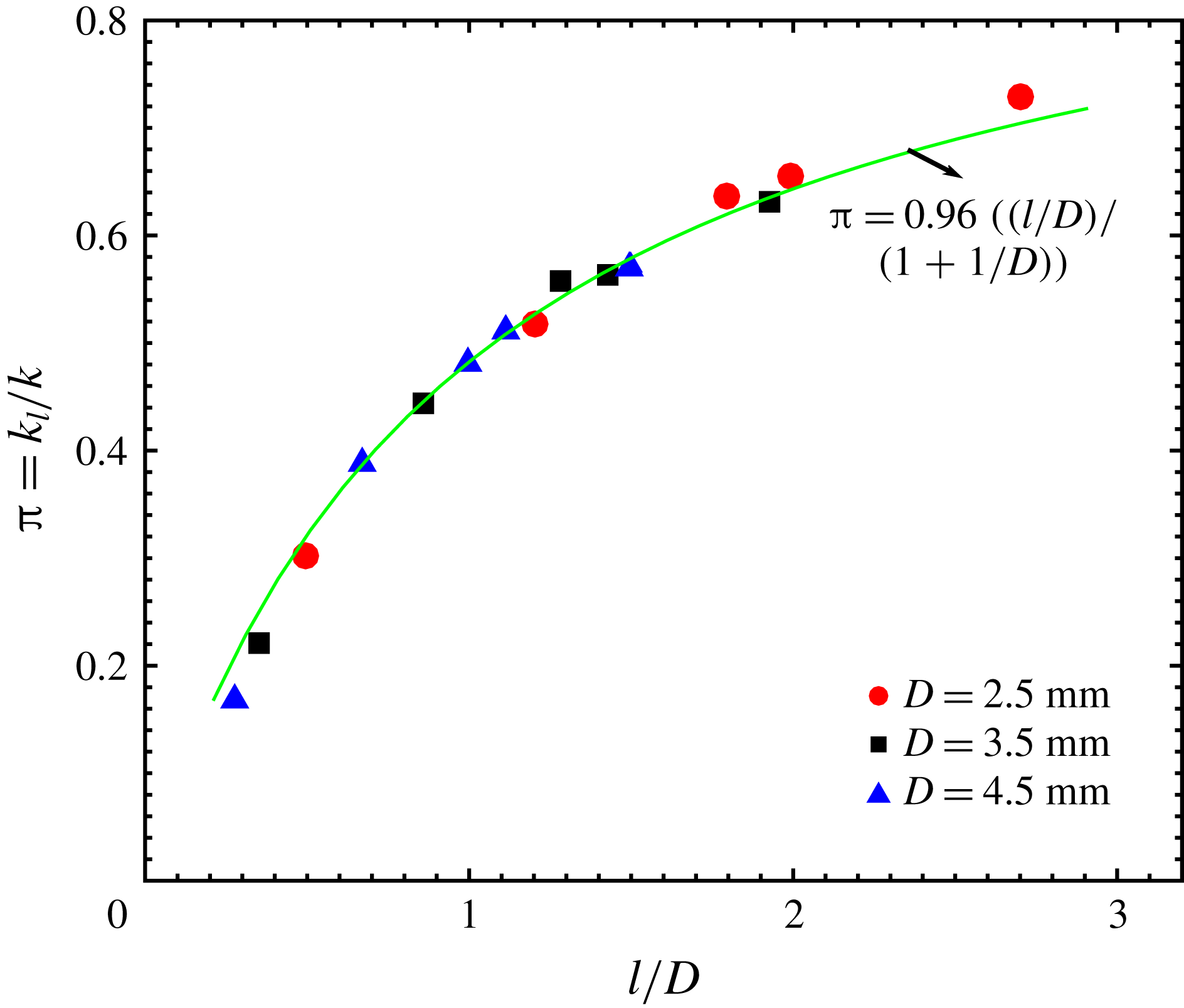
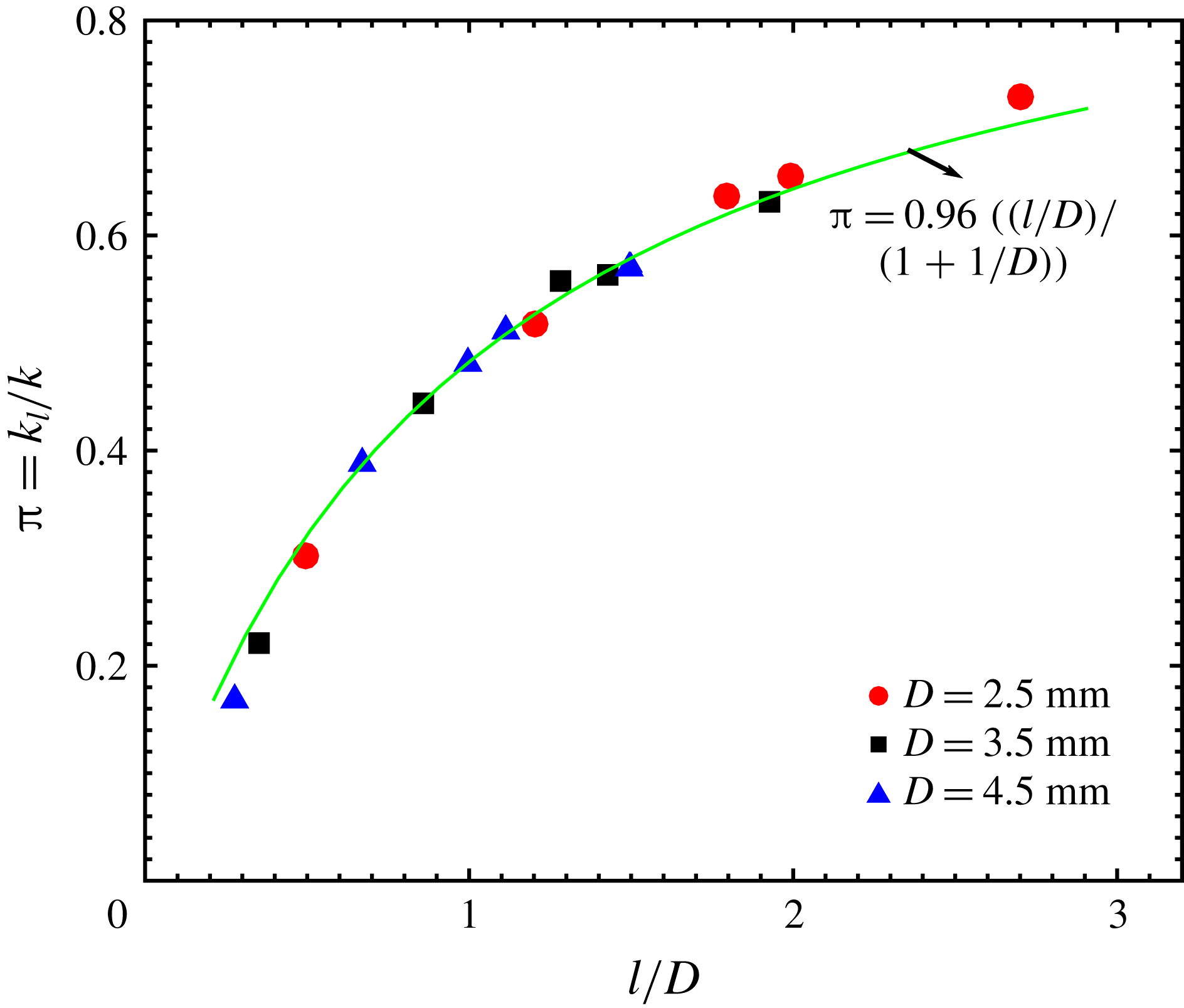
After this validation, we performed the same simulation but limited to the disc layer alone. The simulations were repeated for different configurations. In figure 11, the normalized disc layer permeability
 $\unicode[STIX]{x03C0}=k_{l}/k$
is shown and it matches almost perfectly with the functional form
 $l/(l+D)$
that is related to the fraction of the opening in the disc layer. At the opening between discs, the permeability is still
 $k=b^{2}/12$
, controlled primarily by the gap width
 $b$
. The resulting flow rate
 $u$
through such an opening should be the same as that in a homogeneous case under the same pressure gradient. But the mean flow rate across the disc layer has to average both the opening and impermeable discs
 $\langle u\rangle =ul/(l+D)$
. With the same pressure head and viscosity, it is not surprising that the mean permeability of the disc layer is
 $k_{l}=l/(l+D)k$
.
The normalized disc layer permeability
 $\unicode[STIX]{x03C0}=k_{l}/k$
as a function of the disc layer spacing (
 $l/D$
).
The permeability
 $k_{l}$
is that of the disc layer. If the simulation is extended to the entire cell height with a disc layer inside, the permeability calculated becomes a mean value. Since the disc layer is rather thin, approximately 10 % of
 $H$
, the addition of discs was found to affect the bulk permeability
 $k$
by less than 10 %.