Implications
Dairying contributes significantly to society (employment, economy, nutritional value of dairy products, etc.) at the cost of several environmental impacts. Therefore, improvements in dairy farm ‘eco-efficiency’ are essential to ensure more output with fewer impacts. This study introduced a modelling framework to measure, analyse and understand dairy farm eco-efficiency in much more depth than previously published assessments. The framework was demonstrated with data from French specialized dairy farms. This framework can be a powerful tool for improving the sustainability of dairy farming systems, especially when multiple, conflicting objectives (multiple-output maximization v. multiple-impact minimization) are involved.
Introduction
Facing the environmental impacts (EIs) of agriculture, the challenge to satisfy the demands of a growing and more affluent global population, the scarcity of natural resources and the consequences of climate change, agricultural policies are increasingly directed towards ‘sustainable intensification’ of agriculture (Foresight, 2011). Consequently, the dairy industry (along with other sectors) is required to comply with several policies promoting environmentally sustainable and resource use-efficient production (Casey and Holden, Reference Casey and Holden2005). This necessitates the application of tools to measure dairy farm performance in terms of resource use efficiency and productivity, increased product quantity and value and minimization of EIs. Such a tool is ‘eco-efficiency’, originally developed for the business sector; it is expressed as a ratio of product or service value to EI (Economic and Social Commission for Asia and the Pacific [ESCAP], 2009).
In dairy studies, eco-efficiency is usually expressed as the ratio of an EI per some functional unit such as kg milk or ha land (e.g. Casey and Holden, Reference Casey and Holden2005; van Calker et al., Reference van Calker, Berentsen, Giesen and Huirne2008; Basset-Mens et al., Reference Basset-Mens, Ledgard and Boyes2009; Guerci et al., Reference Guerci, Bava, Zucali, Sandrucci, Penati and Tamburini2013; Bava et al., Reference Bava, Sandrucci, Zucali, Guerci and Tamburini2014). To calculate the EIs dairy studies (including the aforementioned) are increasingly using Life Cycle Analysis (LCA), an internationally standardized method for estimating the EIs of agricultural products from a global perspective (Bava et al., Reference Bava, Sandrucci, Zucali, Guerci and Tamburini2014). Using LCA, some studies have been confined to comparing different dairy systems in terms of several eco-efficiency indicators defined by two or more functional units (e.g. Basset-Mens et al., Reference Basset-Mens, Ledgard and Boyes2009). Others have examined the relationships between eco-efficiency ratios and related factors (e.g. farming intensity, farm self-sufficiency) by employing multivariate methods such as regression (Casey and Holden, Reference Casey and Holden2005) and principal component analysis (Bava et al., Reference Bava, Sandrucci, Zucali, Guerci and Tamburini2014). Other studies have focussed on expressing the relative importance of several eco-efficiency indicators based on different stakeholder weighting schemes (see van Calker et al., Reference van Calker, Berentsen, Giesen and Huirne2008).
There are six main comments to be made on the approaches to dairy farm eco-efficiency in the aforementioned studies. First, analyses involving multiple partial eco-efficiency ratios ignore the substitution possibilities that might exist between different EIs. That is, farms performing moderately for several EIs tend to be overlooked in favour of farms performing exceptionally well for one EI (Kuosmanen and Kortelainen, Reference Kuosmanen and Kortelainen2005). Second, with these ratios the allocation of EIs to products is challenging as dairy farms generally produce other products too, such as meat. Third, incommensurability between several criteria expressed by multiple eco-efficiency ratios rather than a single performance index can complicate decision making (Kuosmanen and Kortelainen, Reference Kuosmanen and Kortelainen2005). Fourth, analyses with methods such as regression and principal component analysis are subject to the method chosen to normalize/standardize eco-efficiency ratios expressed in different units. Fifth, assigning subjective weights to indicators (e.g. the eco-efficiency ratios) has been debated in the literature (Kuosmanen and Kortelainen, Reference Kuosmanen and Kortelainen2005). Sixth, allowance should be made for the fact that there exist factors affecting eco-efficiency that are beyond managerial control, such as the different bio-physical conditions under which farms operate (see Bogetoft and Otto, Reference Bogetoft and Otto2011; Jan et al., Reference Jan, Dux, Lips, Alig and Dumondel2012).
All six aforementioned limitations can be overcome with the productive efficiency method of Data Envelopment Analysis (DEA; see Cooper et al., Reference Cooper, Seiford and Tone2007), employed in this study. DEA is a relative, multiple-input, multiple-output efficiency measurement method calculating single aggregated efficiency indices for each dairy farm by assessing the whole production system, including EIs. Importantly, with DEA no allocation of EIs to specific products is required because the farm is assessed as a whole, multiple-input, multiple-output entity. Most DEA models are not affected by the different measurement units of the data and their weighting schemes are endogenous, that is, ‘data-driven’ (e.g. the model of Cooper et al., Reference Cooper, Park and Pastor1999 employed in this study). DEA methodologies correcting for managerial inefficiencies and accounting for uncontrollable factors are available, such as that of Brockett and Golany (Reference Brockett and Golany1996) adopted in this study.
DEA has been applied in several dairy studies for the calculation of eco-efficiency. For example, Jan et al. (Reference Jan, Dux, Lips, Alig and Dumondel2012) and subsequently Pérez Urdiales et al. (Reference Pérez Urdiales, Oude Lansink and Wall2015) used the DEA eco-efficiency model of Kuosmanen and Kortelainen (Reference Kuosmanen and Kortelainen2005) to define a dairy farm eco-efficiency ratio. This ratio equalled the amount of (physical or monetary) dairy farm output to an aggregate EI index calculated as a weighted summation of all EIs considered in their study. This ratio was then maximized by minimizing the aggregate EIs for the given production levels. Importantly, the EIs in Jan et al. (Reference Jan, Dux, Lips, Alig and Dumondel2012) were LCA-derived. In fact, efficiency studies are increasingly recognizing the advantages of combining LCA with DEA as the former can capture EIs using detailed, cradle-to-grave data (e.g. land use required for the production of feed imported in the dairy farm plus on-farm land use), while the latter has the aforementioned advantages (Vázquez-Rowe and Iribarren, Reference Vázquez-Rowe and Iribarren2015).
The objective of this study was to propose a framework combining LCA with DEA that not only overcomes the six aforementioned issues, but also improves the measurement and understanding of farm eco-efficiency using dairying as exemplar. This will guide farming practice to greater yet sustainable production (sustainable intensification) as advocated for example by the UK Foresight report (2011). The DEA model employed, known as the range adjusted measure (RAM) of inefficiency (Cooper et al., Reference Cooper, Park and Pastor1999), has several desirable properties, for example it allows for the ranking of farms in terms of eco-efficiency performance. Moreover, it seeks to maximize eco-efficiency by simultaneously minimizing EIs and maximizing production. Furthermore, it can identify the factors contributing the most to inefficiency, such as excess EIs and/or under-produced outputs. A method to isolate managerial inefficiency from uncontrollable factors was also demonstrated. That way, it was possible to compare different dairy systems in terms of eco-efficiency solely under the influence of uncontrollable, rather than managerial, factors. The exercise was run using detailed LCA data for French specialized dairy farms. Region was considered as the uncontrollable factor in this study due to the remarkable differences between West and Continental France in terms of farm structure and bio-physical conditions (Gac et al., Reference Gac, Manneville, Raison, Charroin and Ferrand2010b). The results helped identify the eco-efficiency potential of each region and feeding strategy and could therefore aid advisors and policy makers at farm or region/sector level.
Material and methods
Data
LCA was used to estimate several important midpoint impacts of dairy farming systems. It was conducted using the DIAPASON database resulting from a partnership involving voluntary participation of farmers, the Chambers of Agriculture (France) and the French Livestock Institute. This database contains detailed information on technical and economic operations of nearly 500 farms each year throughout France (Charroin et al., Reference Charroin, Palazon, Madeline, Guillaumin and Tchakerian2005).
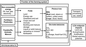
Environmental performance was assessed by indicators of pressure from agricultural activity on the environment considering midpoint impact indicators of LCA. The frontier of the farm system was limited to the farm, considered as a system dedicated to agricultural products (crops, milk, meat) at farm gate. Impacts associated with these products beyond the farm gate were not considered in this study. The limits of the system included the whole farm and all the inputs of the farming system. The system and its main processes are described in Figure 1.
Description of the dairy farming system used for the Life Cycle Analysis (LCA) calculations.

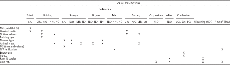
The different EIs considered in this study were midpoint impacts consistent with the CML 2001 methodology (Guinée et al., Reference Guinée, Gorrée, Heijungs, Huppes, Kleijn, Koning de, Oers van, Wegener Sleeswijk, Suh, Udo de Haes, Bruijn de, Duin van and Huijbregts2002) with some specific equations to estimate the emissions. They concern global warming potential and non-renewable energy according to the greenhouse gas emissions GES’TIM methodology (Gac et al., Reference Gac, Deltour, Cariolle, Dollé, Espagnol, Flénet, Guingand, Lagadec, Le Gall, Lellahi, Malaval, Ponchant and Tailleur2010a) and non-renewable energy use (Béguin et al., Reference Béguin, Bonnet, Dollé, Charroin and Ferrand2008) and based on the Fourth Assessment Report of the Intergovernmental Panel on Climate Change (IPCC, 2007). Eutrophication was calculated as a unique impact according to the CML 2001 methodology (Guinée et al., Reference Guinée, Gorrée, Heijungs, Huppes, Kleijn, Koning de, Oers van, Wegener Sleeswijk, Suh, Udo de Haes, Bruijn de, Duin van and Huijbregts2002) and acidification using equations from the European Monitoring and Evaluation Programme/Core Inventory of Air Emissions in Europe (EMEP/CORINAIR, 2002). Table 1 summarizes the inventory of all the emissions considered to calculate the different impacts.
On-farm emissions due to different sources of the farming system

Min.=mineral; N=nitrogen; P=phosphorous; Animal N exc.=animal nitrogen excretion; MS=manure storage; Crop rot.=crop rotation.
The factors applied to the nitrogen (N), phosphorus and carbon fluxes (calculated with the DIAPASON database), generated estimates of EIs. Dry matter intake and mineral excretion in the faeces and urine of animals were calculated according to physiological needs (milk production, weight after calving) using equations proposed by CORPEN (Comité d’orientation pour de pratiques agricoles respectueuses de l’environnement, 1999) taking into account the farmers’ feeding practices (types of forages and concentrates). The carbon (C) storage of permanent grassland that was taken into account was up to 500 kg C/ha per year (Gac et al., Reference Gac, Manneville, Raison, Charroin and Ferrand2010b). On-farm N leaching was estimated using the N farm surplus, including symbiotic fixation (based on a fixed proportion of legumes for permanent grassland), but after removing losses of ammonia and organic N storage in soils assumed as 10% of C storage (with C : N ratio of 10), which represents 50 kg N/ha per year in permanent pasture. The impact values of inputs were derived from the LCA database ‘ecoinvent’ (Nemecek and Kägi, Reference Nemecek and Kägi2007) and Gac et al. (Reference Gac, Deltour, Cariolle, Dollé, Espagnol, Flénet, Guingand, Lagadec, Le Gall, Lellahi, Malaval, Ponchant and Tailleur2010a). Because the whole farm was chosen as the functional unit, all farm products were considered simultaneously in this analysis, therefore no allocation of emissions to the different products was applied.
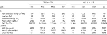
Finally, 185 dairy farms (specialized dairy farms according to the widely recognized Farm Accounts Data Network (FADN) typology) located in different French lowland regions in 2007 and 2008 were kept in this study. The different farms were classified into two main groups according to climate zone and specialization: oceanic specialized systems (OSS; West France, consisting of the following regions: Basse-Normandie, Bretagne, Haute-Normandie, Pays de la Loire, Poitou-Charente) and continental specialized systems (CSS; Continental France, consisting of the following regions: Alsace, Centre, Champagne-Ardenne, Franche-Comté, Lorraine, Rhône-Alpes). The second dimension of the typology, crossed with the first dimension, concerned the type of feeding strategies, based on the area of maize silage in the total forage area of the farm: <10%, 10% to 30%, >30% maize. Other farm classes were not considered due to insufficient number of farms in the class. Table 2 summarizes the five EIs and three outputs used in this study per system for the years 2007 and 2008.
Statistics of dairy farm environmental impacts and outputs per system, in both years 2007 and 2008
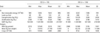
CSS=continental specialized systems; OSS=oceanic specialized systems; EI=environmental impact; GWP=global warming potential.
Data envelopment analysis
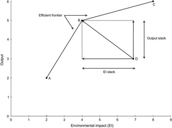
DEA is a non-stochastic, non-parametric technique that benchmarks different decision-making units (DMUs) performing the same task in terms of their capacity to convert inputs into outputs. DEA calculates dimensionless and aggregated efficiency indices without requiring a priori assumptions on the importance of each variable for the DMUs’ performance, making it a particularly attractive multiple-criteria tool. DEA constructs an efficient frontier, that is, a convex, piece-wise linear surface over observed data points against which all DMUs are benchmarked (or ‘enveloped’). Figure 2 represents an efficient frontier ABC for the single-EI, single-output case. The efficient frontier comprises of the best performers (DMUs A, B and C in Figure 2) and the performance of all other DMUs (e.g. DMU D in Figure 2) is evaluated by deviations from the frontier line (Cooper et al., Reference Cooper, Seiford and Tone2007). This is a fundamental difference between DEA and methods such as regression as the latter reflects ‘average’ or ‘central tendency’ behaviour (Cooper et al., Reference Cooper, Seiford and Tone2007) and is unable to provide a holistic characterization of DMUs within a multiple-objective assessment. Convexity in DEA allows for the interpolation from observed DMUs to ‘virtual’ DMUs with input–output profiles between the observations, allowing us to rely on fewer actual observations. These ‘virtual’ DMUs are derived as convex combinations of inputs and outputs of observed DMUs. Convexity can be illustrated in Figure 2 as follows. Any line connecting any two points belonging to, or being placed below, the frontier would also be placed on or below the frontier, and never outside this space (i.e. above the frontier). The points these lines comprise of can represent both observed and ‘virtual’ DMUs. See Bogetoft and Otto (Reference Bogetoft and Otto2011) for a theoretical background on convexity in DEA.
An efficient frontier ABC in the case of a single environmental impact (EI) and a single output. Inefficient decision-making unit D seeks maximal EI reduction and output expansion and thus is projected on ABC at point B.

Data envelopment analysis in the eco-efficiency context
As mentioned in the introduction, eco-efficiency measurement with DEA is advantageous for three main reasons: (i) several EIs are aggregated into a single index, (ii) substitution possibilities between EIs are not left unaccounted for and (iii) no allocation of EIs to specific outputs is required. Points (i) to (iii) can be expressed in the DEA context by minimizing the denominator of the following ratio:
 $${\rm Eco\!-\!efficiency\,{\equals}\,max}\left\{ {{{{\rm Output}} \over {{\rm Weighted}\,{\rm sum}\,{\rm of}\,{\rm EIs}}}} \right\}$$
subject to a number of constraints (see Kuosmanen and Kortelainen, Reference Kuosmanen and Kortelainen2005). In ratio 1 the output can be expressed in monetary or physical terms. The weights summing the various EIs are calculated by the DEA model itself so one need not rely on subjective, pre-defined weight choices for the importance of each EI. Specifically, the DEA model maximizing ratio 1, selects the most self-favourable weights for each DMU so that its eco-efficiency is maximized. These weights cancel out the (often) different measurement units of the EIs, making the DEA model ‘units invariant’ (Cooper et al., Reference Cooper, Seiford and Tone2007).
Despite its usefulness, there are two main limitations with the eco-efficiency DEA model of Kuosmanen and Kortelainen (Reference Kuosmanen and Kortelainen2005). First, ratio 1 can only be maximized by minimizing the EIs for the given output levels. In other words, simultaneous minimization of EIs and maximization of output is not possible. For example, DMU D in Figure 2 would have to move horizontally towards the frontier to become efficient, ignoring any potential increases in its output. Because eco-efficiency expresses the idea of firms (e.g. dairy farms) providing ‘more’ to society with less EIs, it is desirable to use a DEA model allowing for simultaneous adjustments in EIs and output. Second, full eco-efficiency can only be achieved by minimizing all EIs by the same proportion. A DEA model should be able to identify those EIs generating the most detrimental excess (or ‘slack’ in the DEA terminology) to a DMU’s eco-‘inefficiency’.
Both aforementioned limitations can be overcome with the use of so-called ‘additive’ DEA models (see Cooper et al., Reference Cooper, Seiford and Tone2007). These models are able to simultaneously, and non-proportionally, minimize EIs and maximize output for a given DMU. In such a case, DMU D in Figure 2 would move towards point B. The term ‘additive’ is attributed to the fact that these models’ objective functions involve summations of all input and output slacks in order to identify all potential sources of inefficiency. In Figure 2 this summation is represented by the vector heading from point D towards point B and equals the maximal sum of the EI slack and the Output slack. As will be shown below, this summation of all slacks in the objective function departs from the ratio form of ratio 1. However, it is consistent with the idea of maximizing output while minimizing EIs and thus has been adopted in past eco-efficiency studies (see Ramli and Munisamy, Reference Ramli and Munisamy2015 and the related studies they cite). This study employed the RAM additive model (Cooper et al., Reference Cooper, Park and Pastor1999), presented below. RAM and its variants have been used in several eco-efficiency studies of industries other than dairy, see Ramli and Munisamy (Reference Ramli and Munisamy2015).
Range adjusted measure of inefficiency
Suppose that there are n DMUs (e.g. dairy farms) each using m inputs (or EIs in the case of this study) to produce s outputs, denoted as x i (i=1, …, m) and y r (r=1, …, s), respectively. The RAM inefficiency score of the jth DMU, denoted as DMUo, is given by the following linear programme (Cooper et al., Reference Cooper, Park and Pastor1999):
 $$\rho ^{{\asterisk}}\,{\equals}\,\max \nolimits_{{\lambda _{j} ,s_{{io}} ,\,s_{{ro\,}}}} {1 \over {m{\plus}s}}\left( {\mathop{\sum}\limits_{i\,{\equals}1}^m {{{s_{{io}} } \over {R_{i} }}} \,{\plus}\mathop{\sum}\limits_{r\,{\equals}1}^s {{{s_{{ro}} } \over {R_{r} }}} } \right)$$
subject to
 $$\eqalignno{ & x_{{io\,}} \,{\equals}\mathop{\sum}\limits_{j\,{\equals}\,1}^n {x_{{ij}} } \lambda _{{j\,}} {\plus}\,s_{{io}} \,(i\,{\equals}\,1,...,m) \cr & y_{{ro}} \,{\equals}\mathop{\sum}\limits_{j\,{\equals}\,1}^n {y_{{rj}} } \lambda _{j} \,{\minus}\,s_{{ro}} \,(r\,{\equals}\,1,...,s) \cr & \mathop{\sum}\limits_{j\,{\equals}\,1}^n {\lambda _{j} } \,{\equals}1 \cr & \lambda _{j} ,s_{{io}} ,s_{{ro}} \,\geq 0 $$
where x
io
and y
ro
are the inputs and outputs of DMUo respectively; s
io
and s
ro
are the input and output slacks, respectively (Note: input slacks represent overused inputs, i.e. DMUo could have produced the same amount of output using less input. Output slacks represent output shortfalls, i.e. DMUo could have produced more output given its current input use.); λ
j
is a scalar which, when positive, indicates that DMUj has been used as a reference (i.e. benchmark) by DMUo; and R
i
=max
j
{x
ij
}-min
j
{x
ij
}, R
r
=max
j
{y
rj
}−min
j
{y
rj
} represent the ranges in inputs and outputs, respectively, common across all DMUs. The ranges act as a ‘data-driven’ weighting scheme, a more objective one compared to methods where the weights are (subjectively) pre-defined by the user. These weights normalize the slacks and make RAM units invariant. The objective function represents the average proportion of the inefficiencies that the ranges show to be possible in each input and output (Cooper et al., Reference Cooper, Park and Pastor1999). The constraint
 $$\mathop{\sum}\limits_{j{\equals}1}^n {\lambda _{j} } \,{\equals}\,1$$
is the ‘variable returns-to-scale’ specification (see Cooper et al., Reference Cooper, Seiford and Tone2007) which ensures that a farm is only compared to farms of similar size. This specification was desirable in this study as DEA works with absolute values rather than ratios.
Model 2 is run n times, once for each DMU. When DMUo is efficient all its slacks equal zero as this means that it does not need to further reduce its inputs and increase its outputs to become efficient (e.g. DMUs A, B and C in Figure 2). In this case RAM inefficiency ρ* in model 2 equals 0, indicating that DMUo is 100% efficient. If DMUo is inefficient, one can identify through the slack values (which in this case are non-proportional) the inputs and desirable outputs contributing the most to its inefficiency. For an inefficient DMU (e.g. DMU D in Figure 2) any choice of input resulting in
 $$x_{{io}} \,\gt\,\mathop{\sum}\limits_{j{\equals}1}^n {x_{{ij}} \lambda _{j} } $$
means that with some combination of inputs other DMUs (identified by the non-zero λ
j
values) could have improved this input in amount by
 $$s_{{io}} {\equals}\,x_{{io}} {\minus}\mathop{\sum}\limits_{j{\equals}1}^n {x_{{ij}} \lambda _{j} } $$
without worsening any other input or output (Brockett et al., Reference Brockett, Cooper, Golden, Rousseau and Wang2004). Consider, for example a DMU on ABC with coordinates (2.7, 3) as opposed to DMU D with coordinates (7, 3) in Figure 2. The same applies for the desirable outputs and their shortfalls
 $$s_{{ro}} {\equals}\mathop{\sum}\limits_{j{\equals}1}^n {y_{{rj}} \lambda _{j} } \,{\minus}\,y_{{ro}} $$
. In this case consider a DMU with coordinates (7, 5.7) as opposed to DMU D in Figure 2. In either case RAM inefficiency ρ* is greater than 0, indicating that DMUo is inefficient.
Because
 $$\mathop{\sum}\limits_{j{\equals}1}^n {\lambda _{j} } {\equals}1$$
in model 2 it follows that
 $$s_{{io}} {\equals}\mathop{\sum}\limits_{j{\equals}1}^n {\left( {x_{{io}} {\minus}x_{{ij}} } \right)\lambda _{j} } \leq \mathop{\sum}\limits_{j{\equals}1}^n {R_{i} \lambda _{j} } \,{\equals}\,R_{i} $$
and similarly s
ro
⩽R
r
and thus 0⩽ρ*⩽1. Hence, the measure of inefficiency
 $$\rho ^{{\asterisk}} $$
in model 2 can be easily converted to a measure of efficiency as follows:
 $${\rm RAM}\,{\rm efficiency}\,{\equals}\,1{\minus}\,\rho ^{{\asterisk}} $$
RAM efficiency 3 is bounded by 0 and 1. Unity indicates that the DMU under evaluation is efficient while values <1 imply that it is inefficient.
Two very attractive properties of RAM are the following: (i) RAM uses the ranges as a common weighting scheme across all DMUs; and (ii) RAM is strongly monotone in the slacks, that is, holding any other inputs and outputs constant, an increase (decrease) in any of its inputs (outputs) will increase the inefficiency score for an inefficient DMU. Model 1 does not carry properties (i to ii).
Properties (i) to (ii) allow for a full ranking of inefficient DMUs in terms of their RAM efficiency score 3 (Cooper et al., Reference Cooper, Park and Pastor1999). (Not all DEA models carry this property. For example, with ratio 1 one cannot say that a DMU with a score of 0.8 is more eco-efficient than a DMU with a score of 0.7 because the EI weights are DMU-specific and will generally differ between DMUs.) This was strongly desirable in the current study so as to determine whether farms ranked higher in terms of eco-efficiency in a specific region or under a certain feeding strategy.
DEA variables
This study used the five EIs and three outputs in Table 2 for the calculation of eco-efficiency with RAM, namely non-renewable energy use, land use, eutrophication, acidification, global warming potential and milk, meat and crop production. With DEA, increasing the number of variables also increases the number of efficient DMUs which can be quite problematic with small sample sizes. A rough rule of thumb is to choose n⩾max{m×s,3×(m+s)} (Cooper et al., Reference Cooper, Seiford and Tone2007, p. 116). The rule of thumb was satisfied in this study: n=185⩾max{m×s,3×(m+s)}=24.
Testing for differences in eco-efficiency between regions and feeding strategies
Differences in dairy farm eco-efficiency scores between regions and feeding strategies were tested for using the non-parametric Kruskal–Wallis test (see Conover, Reference Conover1999), also known as ‘non-parametric Kruskal–Wallis one-way ANOVA by ranks’ (Sheskin, Reference Sheskin1997). The Kruskal–Wallis test is employed with ordinal (rank-order) data in hypothesis testing involving a design with two or more independent samples (Sheskin, Reference Sheskin1997). That is, dairy farms were ranked in terms of their eco-efficiency scores and differences between groups were tested based on each group’s average rank. The null hypothesis is that all of the populations are identical against the alternative that at least one of the populations tends to yield larger observations than at least one of the other observations (Conover, Reference Conover1999). When at least three groups are compared the Kruskal–Wallis test cannot indicate which pairs of groups significantly differ (provided that significant differences occur). The post-Kruskal–Wallis non-parametric rank test known as Dunn’s test (see Sheskin, Reference Sheskin1997) was therefore employed to identify specific differences between the three feeding strategies.
Choosing non-parametric tests over the parametric one-way ANOVA and its post hoc tests was done for two reasons. First, the theoretical distribution of efficiency scores in DEA is generally unknown so a convention in the DEA literature is to use non-parametric tests (Brockett and Golany, Reference Brockett and Golany1996; Cooper et al., Reference Cooper, Seiford and Tone2007; Bogetoft and Otto, Reference Bogetoft and Otto2011). Second, because RAM can be used to rank DMUs, it lends itself to the rankings that underlie non-parametric rank statistics (Brockett et al., Reference Brockett, Cooper, Golden, Rousseau and Wang2004). Both tests employed in this study operate based on the rank transformation approach; that is, the data are replaced by their ranks and then the usual parametric tests (e.g. t test, F test, etc.) are applied on the ranks. (Tied observations [e.g. when at least two DMUs are eco-efficient] are given the average rank of the tied scores.) Therefore, these tests are not affected by outliers or skewed data. See Conover (Reference Conover1999).
Examining the effect of region on eco-efficiency
The bio-physical conditions under which dairy farms operate largely differ between West and Continental France. Regional differences in eco-efficiency were therefore tested. It would seem appropriate to pool farms from both regions in one dataset, run the RAM model and then test for differences between regions with the Kruskal–Wallis test. Such practice, however, would reveal any differences between regions under the observed levels of EIs and output (i.e. the EI and output values outlined in Table 2). This means that inefficiencies attributed to both managerial and regional factors would not allow inefficient farms to operate under their full potential. Indeed, the risk of amalgamating both sources of inefficiency (managerial and regional) is to grant inadvertently some bad managers (farmers) good eco-efficiency scores when they are only benefitting from operating under particularly favourable bio-physical conditions (see Brockett and Golany, Reference Brockett and Golany1996). Removing EI and output managerial inefficiencies (i.e. slacks) was therefore essential before comparing the two regions in terms of eco-efficiency. This was done by adopting the methodology of Brockett and Golany (Reference Brockett and Golany1996) which involved the following four steps:
-
1. Run two separate DEA exercises, one for CSS only and one for OSS only with model 2.
-
2. Using the optimal EI and output slacks obtained from the previous step make the necessary reductions in EIs and outputs so that inefficient DMUs in each group become efficient. This is done using the following formulas:
 $$\eqalignno{ & \hat{x}_{{io}} \,{\equals}\,x_{{io}} \,{\minus}\,s_{{io}}^{{\asterisk}} \,\left( {i\,{\equals}\,1,...,\,m} \right) \cr & \hat{y}_{{ro}} \,{\equals}\,y_{{ro}} {\plus}s_{{ro}}^{{\asterisk}} \,\left( {r\,{\equals}\,1,...,\,s} \right) $$
where the asterisks (*) denote optimality. (For example, let us assume that Figure 2 represents OSS farms. With formulas 4 the OSS farm D would have been projected onto the OSS efficient frontier at point B.) Now managerial inefficiency has been eliminated within OSS and CSS and both are operating ‘up to the boundary of the capabilities which the evidence showed was possible for [OSS and CSS]’ (Cooper et al., Reference Cooper, Seiford and Tone2007, p. 238).
-
3. Pool all DMUs deriving from the previous step and run a new DEA exercise with model 2.
-
4. Test for significant differences between the systems’ efficiency scores using non-parametric rank statistics, i.e. the Kruskal–Wallis test.
Following the steps above it was possible to compare the two regions in terms of eco-efficiency. It should be noted, however, that the DMUs were then evaluated not based on their actual levels of EIs and output, but on their efficient ones. Because this methodology corrects for any managerial inefficiencies present in DMUs, from this point it is referred to as the ‘corrective’ methodology.
Putting all methods together
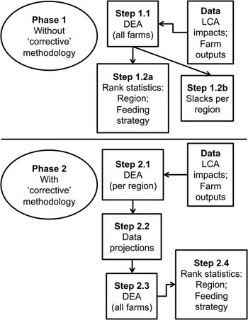
Figure 3 summarizes the methodology employed in this study. Phase 1 did not apply the ‘corrective’ methodology and involved two steps. In Step 1.1 the EIs and outputs for each farm were fed into RAM and the eco-efficiency scores were obtained. Note that in this step DMUs from both CSS and OSS were pooled before the RAM was run. Step 1.2a tested for differences in eco-efficiency scores between the two systems and between the three feeding strategies with non-parametric rank tests. Moreover, the EI and output slacks were compared between systems in Step 1.2b. Phase 2 applied the ‘corrective’ methodology and involved four steps. In Step 2.1 the RAM model was run for each system (CSS, OSS). In Step 2.2 the EIs and outputs of each farm in each system were projected onto their efficient levels with the formulae in 4. In Step 2.3 the RAM model was re-run for the whole sample (both CSS and OSS) using the projected data from Step 2.2. Step 2.4 tested for differences in the new eco-efficiency scores between the two systems and between the three feeding strategies with non-parametric rank tests. Unlike Phase 1, in Phase 2, systems and feeding strategies were exposed to the full eco-efficiency potential that the data showed to be possible for these groups.
Description of the modelling framework adopted in this study. DEA: Data Envelopment Analysis. LCA=Life Cycle Analysis.

There are distinct differences between Phase 1 and 2. Although Phase 1 did not differentiate between regional and managerial factors, it helped to evaluate the 185 French specialized farms under their observed levels of EIs and outputs, as reported in Table 2. In other words, Phase 1 evaluated farms ‘as they actually performed’ and not ‘as they could be performing’, as in the ‘corrective’ methodology described in Phase 2. Phase 1 is therefore useful for efficiency comparisons between and within farms in terms of the whole population, without correcting for potential systematic differences between groups (defined by region in this case). Phase 2 is appropriate for testing the hypothesis that systematic unavoidable differences between groups will affect efficiency performance. Phases 1 and 2 are therefore independent but complementary. See Brockett et al. (Reference Brockett, Cooper, Golden, Rousseau and Wang2004) who also conducted their analysis in two stages analogous to the two Phases employed here.
All calculations were run with the R language (http://www.R-project.org/). The R function for RAM was developed by the first author of this article. The Kruskal–Wallis test is available in the standard version of R. Dunn’s test is available by the R package ‘dunn.test’ (https://cran.r-project.org/web/packages/dunn.test/dunn.test.pdf).
Results
Eco-efficiency scores and slacks per system and feeding strategy when accounting for managerial inefficiencies
The results for the eco-efficiency scores and slacks presented in this sub-section were calculated before applying the ‘corrective’ methodology (Phase 1 in Figure 3).
Eco-efficiency scores
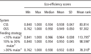
Statistics for the eco-efficiency scores and their mean ranks per system and feeding strategy are presented in Table 3. The mean, median and mean ranks of eco-efficiency scores were higher for OSS than CSS. However, the Kruskal–Wallis test did not identity significant differences between CSS and OSS in terms of the eco-efficiency scores’ mean ranks (P=0.105). The three feeding strategies ranked as follows in terms of mean, median and mean ranks of eco-efficiency scores: (<10% maize)>(10% to 30% maize)>(>30% maize). The Kruskal–Wallis test identified significant differences between the three feeding strategies in terms of the eco-efficiency scores’ mean ranks (P=0.001). Specific differences were identified with Dunn’s test. Differences were significant between DMUs with <10% maize and >30% maize in the total forage area (P<0.001) and between DMUs with 10% to 30% maize and >30% maize (P=0.011). No differences were found between DMUs with >10% maize and 10% to 30% maize in the total forage area (P=0.083).
Statistics for eco-efficiency scores per system and feeding strategy before removal of managerial inefficiencies

CSS=continental specialized systems; OSS=oceanic specialized systems.
a,bValues within a column with different superscripts differ significantly at P<0.05.
1 Maize area as % of total forage area on farm.
EI and output slacks
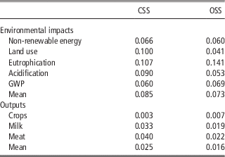
Table 4 summarizes the optimal EI and output slacks from model 2 per system, expressed as proportions of their respective ranges i.e.
 $${{s_{{io}}^{{\asterisk}} } \mathord{\left/ {\vphantom {{s_{{io}}^{{\asterisk}} } {R_{i} }}} \right. \kern-\nulldelimiterspace} {R_{i} }}\,\,\left( {i\,{\equals}\,1,...,\,m} \right)$$
and
 $${{s_{{ro}}^{{\asterisk}} } \mathord{\left/ {\vphantom {{s_{{ro}}^{{\asterisk}} } {R_{r} }}} \right. \kern-\nulldelimiterspace} {R_{r} }}\,\,\left( {r\,{\equals}\,1,...,\,s} \right)$$
. That way, it was possible to ‘decompose’ the eco-efficiency scores in Table 3 in order to detect the EIs and outputs with the highest relative contribution to a DMU’s inefficiency. (Averaging each system’s input and output inefficiencies in Table 4 and then subtracting them from 1 equals the mean efficiency scores presented in Table 3.) The EIs with the highest contribution to CSS systems’ inefficiency were eutrophication potential, land use and acidification potential. By contrast, eutrophication potential was the EI with the by-far-largest contribution to OSS systems’ inefficiency. In terms of output inefficiency, meat and milk were by far the largest contributors to the inefficiency of both OSS and CSS. Notably, for both OSS and CSS the mean input inefficiencies were much higher than the mean output inefficiencies.
Mean slack values per system expressed as a proportion of their corresponding ranges

CSS=continental specialized systems; OSS=oceanic specialized systems; GWP=global warming potential.
Eco-efficiency scores per system and feeding strategy after eliminating managerial inefficiencies
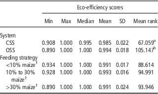
The eco-efficiency results per system and feeding strategy presented in this section were obtained after eliminating all managerial inefficiencies (i.e. slacks) from the 59 CSS farms and 126 OSS farms, based on the ‘corrective’ methodology (Phase 2 in Figure 3). Statistics for the eco-efficiency scores and their mean ranks per system and feeding strategy are presented in Table 5. The mean and mean ranks of eco-efficiency scores were higher for OSS than CSS and the medians of both systems equalled 1. The Kruskal–Wallis test identified significant differences between the eco-efficiency scores’ mean ranks of the two systems (P<0.001). The three feeding strategies had almost-equal mean and equal median eco-efficiency scores. The Kruskal–Wallis test did not identify significant differences between feeding strategies in terms of mean ranks of the eco-efficiency scores (P=0.767).
Statistics for eco-efficiency scores per system and feeding strategy after removal of managerial inefficiencies

CSS=continental specialized systems; OSS=oceanic specialized systems; GWP=global warming potential.
a,bValues within a column with different superscripts differ significantly at P<0.05.
1 Maize area as % of total forage area on farm.
Discussion
This study is aimed at researchers, advisors and policy makers searching for tools that can address the challenges of increasing farm output and reducing EIs, especially given the recent trend towards sustainable intensification of agriculture (see Foresight, 2011). Our framework contributes to the stream of literature employing methodologies able to capture several aspects in order to ensure that development is in fact ‘sustainable’. Dairy farming was used as an exemplar to demonstrate the framework, which is expandable to other agricultural settings.
Not ‘just LCA’ but ‘DEA and LCA’
According to recent guidelines by the Livestock Environmental Assessment and Performance Partnership (LEAP, 2015, p. 6), ‘[i]n order to prevent shift of burden from [one] environmental issue to another, no environmental improvement option should be recommended without having […] assessed […] the effects on resource use and those other EIs targeted as relevant for livestock supply chains […]’. In other words, the LEAP guidelines themselves implicitly acknowledge the issue of substitution possibilities between LCA eco-efficiency ratios, mentioned in the introduction to this study. The implications of this issue can be demonstrated by looking at the results of LCA eco-efficiency studies comparing dairy farms with different proportions of land devoted to maize silage (e.g. Basset-Mens et al., Reference Basset-Mens, Ledgard and Boyes2009; Rotz et al., Reference Rotz, Montes and Chianese2010). According to these studies, because grassland requires less fertilization than arable land, lower impacts from eutrophication, acidification, greenhouse gas emissions and non-renewable energy use have been observed on grass-based farms. However, arable crops such as maize silage have higher yields per hectare. It is therefore impossible to conclude that a particular feeding strategy has a higher eco-efficiency potential than another one, unless all feeding strategies are evaluated at the aggregate level, as was done in this study. Indeed, feeding the LCA variables into the RAM model showed that the eco-efficiency of farms with >30% maize was lower, favouring more grass-based systems.
Regional differences
Higher eco-efficiency scores were expected for OSS systems over CSS because the bio-physical conditions in West France are more favourable. Specifically, the climate conditions in West France favour the production of high quality forages which are essential for dairy production. These differences in climate conditions between West and Continental France were implicitly examined in this study by removing managerial inefficiencies from CSS and OSS with the ‘corrective’ methodology. Indeed, Jan et al. (Reference Jan, Dux, Lips, Alig and Dumondel2012) emphasized that DEA results should be interpreted with care as inefficiencies may be attributed to factors that are beyond managerial control. Hence, removing managerial factors with the ‘corrective’ methodology revealed each system’s true eco-efficiency potential that the projected data showed to be possible, solely as a result of the different bio-physical conditions between West and Continental France. OSS systems then ranked significantly higher, on average, than CSS in terms of eco-efficiency scores (Table 5).
Identifying specific sources of eco-‘inefficiency’
Examining the slacks (Table 4) can help prioritize the reduction (increase) of those EIs (outputs) most responsible for the eco-inefficiency of CSS and OSS. For example, CSS systems had a quite large acidification slack. In fact, in CSS systems cows are generally offered more protein concentrates, potentially to avoid any protein shortages, which tends to increase ammonia emissions (Faverdin et al., Reference Faverdin, Baratte, Perbost, Thomas, Ramat and Peyraud2014). It is noteworthy that CSS also had a large land use slack (Table 4). These systems devoted a larger part of on-farm land to crop production at the expense of lower milk and meat production than OSS (compare mean crops-milk and crops-meat ratios per system, which can be easily derived from Table 2). This, in turn, explains the lower crops slack, and higher milk and meat slacks, of CSS in comparison with OSS (Table 4). Finally, note that for both systems the largest slack was eutrophication, as opposed to the relatively low global warming potential slacks. This agrees with the findings of Bava et al. (Reference Bava, Sandrucci, Zucali, Guerci and Tamburini2014) that livestock systems are often responsible for important local EIs.
Methodological aspects
Eco-efficiency as a relative measure to improve sustainability
It can be argued that improving eco-efficiency does not guarantee sustainability. Because eco-efficiency is a relative measure, improvements can be achieved if either EIs are reduced or outputs are increased. Furthermore, the absolute environmental pressure can still exceed the ecosystem’s carrying capacity (Kuosmanen and Kortelainen, Reference Kuosmanen and Kortelainen2005). For example, there is a high concentration of dairy farms in West France and the main production regions are located near environmentally sensitive areas (Chatellier and Pflimlin, Reference Chatellier and Pflimlin2006). Thus, although OSS systems had higher eco-efficiency, this does not necessarily mean that they operated within the local ecosystem’s carrying capacity.
Nevertheless, eco-efficiency is often cost-effective so it makes economic sense to exploit it to the utmost (Kuosmanen and Kortelainen, Reference Kuosmanen and Kortelainen2005). In this study the RAM model helped identify such options through the relative EI and output slacks (Table 4). Prioritizing those EIs and outputs with the largest relative slacks can result in notable eco-efficiency improvements. This is advantageous because policies targeted at eco-efficiency improvements tend to be easier to adopt, and politically easier to implement, than policies restricting the level of economic activity (Kuosmanen and Kortelainen, Reference Kuosmanen and Kortelainen2005).
Comparing RAM with alternative methods
This study considered RAM’s ranking property as one of its main advantages. Besides RAM, there are several promising methods to rank DMUs. See the reviews by Adler et al. (Reference Adler, Friedman and Sinuany-Stern2002) and Markovits-Somogyi (Reference Markovits-Somogyi2011) regarding the methods mentioned hereafter. Other ranking methods missing from both reviews exist, such as the ‘global efficiencies’ (GLE) approach by Despotis (Reference Despotis2002) which, like RAM, uses a common weighting scheme across all DMUs. These ranking methods can be roughly classified as having at least one of the following characteristics: (i) they require modifications to the original DEA model (e.g. when imposing weights restrictions); (ii) they involve supplementary analyses with tools such as multivariate statistics (e.g. canonical correlation analysis for ranking) or multiple-criteria decision making (e.g. GLE), which translates to additional computational time and/or coding effort; (iii) the original DEA model cannot be easily solved (e.g. fuzzy DEA); and (iv) there is no correspondence between the DMUs’ efficiency scores and their ranks (e.g. GLE). While some of these issues can be dealt with fairly easily (e.g. the weights restrictions), to the best or our knowledge, RAM is the only simple, readily available linear DEA model with a ranking property that does not involve (i to iv). Note that RAM can only rank inefficient DMUs. In fact, ranking efficient DMUs was not desirable here because rankings can differ between methods (see Adler et al., Reference Adler, Friedman and Sinuany-Stern2002), possibly affecting the results of the non-parametric rank statistics.
Additive models (such as RAM) are not the only DEA models able to simultaneously minimize EIs (and/or inputs) and maximize output. Another example is the directional distance function (DDF) whereby the minimization of EIs and inputs, and maximization of outputs, is made via a ‘direction vector’ that reflects different stakeholder preferences. For example, the direction vector may be set to minimize EIs for the given outputs, maximize outputs for the given EIs or do both simultaneously. Several other choices are also possible (see Beltrán-Esteve et al., Reference Beltrán-Esteve, Picazo-Tadeo and Reig-Martínez2014; Berre et al., Reference Berre, Blancard, Boussemart, Leleu and Tillard2014). For instance, Berre et al. (Reference Berre, Blancard, Boussemart, Leleu and Tillard2014) argued that a sustainable intensification scenario would seek to reduce pollution and increase outputs with a possible increase in inputs. The RAM model can also allow for input increases because it can handle negative values (see Cooper et al., Reference Cooper, Park and Pastor1999): simply assign a negative sign to the inputs to be increased.
DDFs are advantageous over RAM when the objective is not only to calculate the input and output adjustments necessary for a DMU to operate efficiently, but also to determine how ‘far’ these adjustments are from an input–output combination maximizing profits (provided that input and output prices are known) for this particular DMU (Färe and Grosskopf, Reference Färe and Grosskopf2000). This ‘allocation’ problem cannot be modelled with RAM. Nonetheless, RAM is appropriate when it is desirable to decompose efficiency scores into variable-specific scores through the slacks (as was done here) because, unlike DDFs, RAM does not assume proportional adjustments in inputs and outputs (some recently developed DDFs that relax this assumption have in fact an additive structure; see Chen et al., Reference Chen, Yu, Chang, Hsu and Managi2015). Note that there are several normalization options for the slacks (other than by division by the variables’ ranges as was done here) that create opportunities for further analyses (Cooper et al., Reference Cooper, Park and Pastor1999 discuss a range of choices). For example, when input prices are known, input slacks can be ‘priced’ to determine the proportion of each input’s cost to the total cost (see Soteriades et al., Reference Soteriades, Faverdin, March and Stott2015).
Finally, we draw attention to the alternative definitions of ‘data-driven’ weights in models 1 and 2. In model 1 the weights are calculated by the model itself. This may result in large weights for EIs of secondary importance, leaving a negligible or zero weight for more important EIs (Kuosmanen and Kortelainen, Reference Kuosmanen and Kortelainen2005). This can be fixed by restricting a priori the weights’ values to admissible ranges (see Kuosmanen and Kortelainen, Reference Kuosmanen and Kortelainen2005). By contrast, with RAM (model 2) the weights are not calculated but given, because the model uses the variable’s ranges as weights, which are always non-zero. Therefore, reliance on subjective weights restrictions as in model 1 is not necessary with RAM.
Choice of DEA variables
Choice of input and output variables used is a key aspect of DEA methodology. Past studies on dairy farm eco-efficiency with DEA often use one aggregate output indicator to avoid too many DMUs on the efficient frontier. For example, Pérez Urdiales et al. (Reference Pérez Urdiales, Oude Lansink and Wall2015) defined output as economic value added [(milk sales+value of on-farm consumption of milk) – direct costs]. On the other hand, Jan et al. (Reference Jan, Dux, Lips, Alig and Dumondel2012) argued that economic value added might bias the results as an increase in the market price of a given commodity would lead to higher eco-efficiency. Instead, they aggregated all farm outputs into a single output of digestible energy content. However, with this method it is assumed that any form of energy in human diets can be substituted by any other, provided that energy requirements are met. Also, milk, meat and crops have different nutritional values in addition to energy content. Therefore, in this study it was deemed more appropriate to keep milk, meat and crops as three separate outputs.
Furthermore, in this study the eco-efficiency measure did not include operational inputs (e.g. labour, capital, on-farm electricity use) and ‘undesirable’ outputs (e.g. kg CO2-equivalents, wastewater) because the idea was to aggregate altogether the two elements used in LCA ratios: EIs and outputs. In other words, we were concerned with the EIs rather than the amount of operational inputs and undesirable outputs of DMUs (see Jan et al., Reference Jan, Dux, Lips, Alig and Dumondel2012, p. 715, but also Kuosmanen and Kortelainen, Reference Kuosmanen and Kortelainen2005). An alternative way of conducting eco-efficiency analysis by also involving operational inputs and undesirable outputs is with the ‘LCA+DEA method’ (see Vázquez-Rowe and Iribarren, Reference Vázquez-Rowe and Iribarren2015). With LCA+DEA, ‘target’ LCA impacts are obtained by adjusting the operational inputs to their optimal values via DEA and re-performing the LCA exercise. Therefore, in LCA+DEA the DEA exercise is an intermediate step that helps determine the DMUs’ benchmarks and thus the target EIs. Alternatively, target EIs can be obtained directly from RAM’s optimal slacks. This reduces potential dimensionality issues because the set of DEA variables will generally be smaller than that with LCA+DEA (Jan et al., Reference Jan, Dux, Lips, Alig and Dumondel2012, p. 715).
Conclusion
Combining LCA with RAM, the ‘corrective’ methodology and non-parametric rank tests can significantly improve (dairy) farm eco-efficiency assessments compared to previous studies using partial ratios or coupling LCA with DEA. The modelling framework was demonstrated with LCA data for French specialized dairy farms. Results showed that OSS systems ranked higher, on average, than CSS systems in terms of eco-efficiency. Also, the average eco-efficiency rank of farms with lower proportions of maize silage in the total forage area was higher, on average, than farms with higher proportions of maize. These results helped identify the eco-efficiency potential of each region and feeding strategy and could therefore aid advisors and policy makers at farm or region/sector level. This demonstration also highlights the capacity of the proposed multiple-EI, multiple-output framework to measure and understand eco-efficiency, and to compare different groups, which makes it a promising multiple-criteria tool towards the achievement of greater yet sustainable agricultural production.
Acknowledgements
The authors would like to express their gratitude to two anonymous referees whose constructive comments helped significantly improve an earlier version of this manuscript. The authors take responsibility for any errors that may remain. We acknowledge feedback from staff at SRUC (Scotland), INRA (St Gilles, France) and Idele (Le Rheu, France) and also from Dr Philippe Lecomte (CIRAD, France) and Dr Marc Metzger (University of Edinburgh). Likewise, thank you to Professor Mette Asmild (University of Copenhagen) and Professors Jean-Philippe Boussemart and Hervé Leleu at IÉSEG (Lille, France) for the fruitful discussions on DEA, as well as to Dr Jiayi Liu and Dr Giles Innocent (BioSS, Scotland) for their tips in statistics. This project is jointly funded by SRUC (via Scottish Government’s Rural Affairs and the Environment Strategic Research programme) and the PHASE division of INRA.