1. Introduction
In this study our concern is with the properties of barotropic azimuthally propagating vorticity waves in a circular polar basin. The basin is taken to have an axisymmetric continental shelf topography and this allows us to develop analytical approximations for the eigenfrequencies of the propagating waves. The problem considered in this paper is a natural extension of a recent study (Bassom & Willmott Reference Bassom and Willmott2019) in which we derived accurate approximations for the eigenfrequencies of planetary waves in a flat bottom polar basin. As noted by LeBlond (Reference LeBlond1964), the analytical treatment of the ocean dynamics near the pole is frustrated by the quadratic dependence of the Coriolis parameter with co-latitude. To our knowledge, the only analytical treatment of topographic Rossby waves in a circular polar basin on a sphere was undertaken by LeBlond (Reference LeBlond1964). That study focussed on the special case of an axisymmetric sloping bottom with co-latitudinal dependence identical to that of the Coriolis parameter, thereby greatly simplifying the analysis on the polar plane. LeBlond (Reference LeBlond1964) demonstrated that the sign and magnitude of the slope determine the direction of propagation of the planetary waves, which we recognise is due to the well known ‘topographic beta mechanism’ operating on the polar plane.
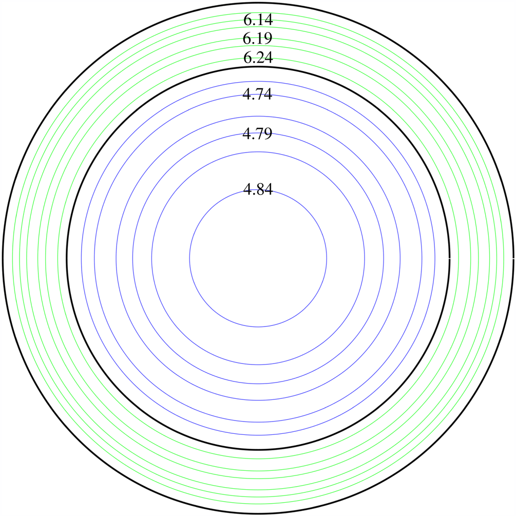
The topography considered by LeBlond (Reference LeBlond1964) is a somewhat unrealistic representation of a continental shelf because the bottom slopes from the centre of the basin to its boundary. A more natural representation of a continental shelf is an axisymmetric step shelf of uniform width and depth that is adjacent to a uniform deep basin. This is the choice of topography adopted in this paper. Figure 1 depicts contours of the planetary potential vorticity field  $\Pi _P=f(\theta )/H(\theta )$ associated with a step shelf where
 $f$ is the Coriolis parameter,
 $H$ is the undisturbed ocean depth and
 $\theta$ the co-latitude. On the shelf and in the deep basin
 $\Pi _P$ increases poleward. However, there is a jump in the value of
 $\Pi _P$ upon crossing the step due to the discontinuous change in depth such that
 $\Pi _P^{S}(\theta )>\Pi _P^{D}(\theta )$, where the superscripts
 $S$ and
 $D$ refer to the fields on the shelf and in the deep basin, respectively. Here, we are considering the oceanographically relevant case where the depth of the deep basin exceeds that of the shelf. Clearly, the planetary potential vorticity field plotted in figure 1 supports two families of vorticity waves; planetary waves associated with
 $\Pi _P^{S}$ and
 $\Pi _P^{D}$ increasing poleward and topographic Rossby waves, more appropriately referred to as ‘shelf waves’ for the choice of topography in this study, supported by the jump in the value of
 $\Pi _P$ at the step.
Contours of  $\Pi _P = 2\Omega \cos \theta /H(\theta )$ for the step shelf (3.1) with the parameter choices
 $H_1 = 2250$ m,
 $H_2 = 3000$ m,
 $\theta _S = {\rm \pi} /12$ and
 $\theta _B = {\rm \pi} /9$.

Following our earlier analysis developed in Bassom & Willmott (Reference Bassom and Willmott2019), we shall employ asymptotic methods to calculate series for the topographic Rossby wave eigenfrequencies. The results are based on the latitudinal limit of the polar basin which constitutes a natural small parameter in the problem. We anticipate that the leading-order term will correspond to the topographic Rossby wave frequencies for a step shelf in a uniformly rotating basin, albeit modified by the spherical geometry. At the next order we demonstrate that a planetary wave correction term appears associated with the variation of the Coriolis parameter with co-latitude.
The Arctic Ocean basin is unique in supporting a planetary potential vorticity field of the type shown qualitatively in figure 1. Nøst & Isachsen (Reference Nøst and Isachsen2003) plot contours of the actual  $f/H$ in the Arctic basin which reveals that the two deep basins, Canada and Eurasian, are bounded by closed planetary potential vorticity contours which qualitatively are captured by the
 $f/H$ field contoured in figure 1. However, the picture revealed by Nøst & Isachsen (Reference Nøst and Isachsen2003) is complicated by the presence of the subsurface Lomonsov Ridge that separates the two deep basins. In reality, the two basins might individually support their own set of topographic wave modes. Nevertheless, as a starting point for the analysis of shelf waves in a spherical polar cap it is logical to adopt the simple step-shelf profile.
Intriguingly, topographic Rossby waves have been detected in the analysis of time series of temperature and horizontal velocity in the Beaufort Gyre of the Arctic Ocean by Timmermans et al. (Reference Timmermans, Rainville, Thomas and Proshutinsky2010) and Zhao & Timmermans (Reference Zhao and Timmermans2018). The waves have periods of some tens of days which they suggest is consistent with the theory of Rhines (Reference Rhines1970) for bottom trapped Rossby waves in a continuously stratified fluid over a small linear sloping bottom on an  $f$-plane. In the final section of this paper we will reconsider the interpretation of these observed shelf waves in the light of the theory developed in this study.
The remainder of the paper is structured as follows. The eigenvalue problem is formulated presently in § 2 which is then analysed to develop a two-term asymptotic approximation for the eigenfrequencies of topographic Rossby waves over a step. This calculation is described in § 3 while the results and discussion conclude the paper in § 4.
2. Formulation
Consider an ocean with an axisymmetric depth profile centred at the pole; in terms of a spherical coordinate system in which  $\theta$ and
 $\varphi$ denote the co-latitude and longitude, respectively, the basin is defined by
 $0\leq \theta \leq \theta _B$,
 $0\leq \varphi \leq 2{\rm \pi}$. If the unit vectors
 $(\widehat {\boldsymbol {k}}, \widehat {\boldsymbol {\theta }},\widehat {\boldsymbol {\varphi }})$ form a right-handed triad so that
 $\widehat {\boldsymbol {k}}$ points in the outward radial (locally upward) direction, the linearised shallow-water equations for the inviscid homogeneous dynamics within the polar cap are
 \begin{align} u_t+fv=-\frac{g}{R\sin\theta}\eta_\varphi,\quad v_t-fu=-\frac{g}{R}\eta_\theta,\quad \eta_t+\frac{1}{R\sin\theta}[(Hu)_\varphi +(Hv\sin\theta)_\theta]=0, \end{align}
here, the velocity 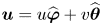 $\boldsymbol {u}=u\widehat {\boldsymbol {\varphi }}+v\widehat {\boldsymbol {\theta }}$,
 $\eta$ is the free-surface elevation of the ocean,
 $R$ is the radius of the Earth,
 $g$ denotes the gravitational acceleration and
 $f=2\Omega \cos \theta$ where
 $\Omega$ is the angular velocity of the Earth. Azimuthally propagating wave solutions of (2.1) are sought in the form
 \begin{equation} (u,v,\eta)=(U(\theta),V(\theta),F(\theta))\exp[\textrm{i}(m\varphi-\omega t)], \end{equation}
in which the wavenumber  $m$ is an integer,
 $\omega$ is the angular frequency and
 $U$,
 $V$ and
 $F$ are amplitude functions. If the expressions (2.2) are substituted into system (2.1) it is found that
 \begin{equation}-\textrm{i}\omega U+fV=-\frac{\textrm{i}mg}{R\sin\theta}F,\quad -\textrm{i}\omega V-fU=-\frac{g}{R}\frac{\textrm{d} F}{\textrm{d}\theta} \end{equation}
and
 \begin{equation} -\textrm{i}\omega R\sin\theta F+\textrm{i}mHU+\frac{\textrm{d}}{\textrm{d}\theta}(HV\sin\theta)=0. \end{equation}
If we eliminate  $U$ and
 $V$ from system (2.3) in favour of
 $F$ we are led to
 \begin{align} &\frac{\textrm{d}^{2}F}{\textrm{d}\theta^{2}}+\left( \frac{\sin 2\theta}{\cos^{2}\theta-\sigma^{2}}+\cot\theta+\frac{H'}{H}\right)\frac{\textrm{d}F}{\textrm{d}\theta}\nonumber\\ &\quad-\left[\frac{m}{\sigma}\left(\frac{\cos^{2}\theta+\sigma^{2}}{ \cos^{2}\theta-\sigma^{2}}\right)+\frac{m^{2}}{\sin^{2}\theta}+\left(\frac{R}{r_e}\right)^{2} (\cos^{2}\theta-\sigma^{2})+\frac{m}{\sigma\tan\theta}\frac{H'}{H}\right]F=0. \end{align}
In (2.4),  $\sigma =\omega /2\Omega$ is the dimensionless frequency while
 $r_e=(2\Omega )^{-1}\sqrt {gH}$ is the external Rossby radius of deformation. The associated boundary conditions arise from the demand that there be no normal velocity
 $V=0$ at the basin edge
 $\theta =\theta _B$ and that solutions are not singular at the pole
 $\theta =0$; written in terms of
 $F$ these requirements become
 \begin{equation} F(0)=0\quad\textrm{and}\quad F'-\frac{m}{\sigma}\cot\theta\, F=0\quad \textrm{at}\ \theta=\theta_B. \end{equation}
It is worth remarking on the simplification that occurs in the case of a uniformly rotating polar basin for which  $f=2\Omega$. Then (2.4) reduces to
 \begin{equation} \frac{\textrm{d}^{2}F}{\textrm{d}\theta^{2}}+\left(\cot\theta+\frac{H'}{H}\right)\frac{\textrm{d}F}{\textrm{d}\theta} -\left[\frac{m^{2}}{\sin^{2}\theta}+\left(\frac{R}{r_e}\right)^{2}(1-\sigma^{2})+ \frac{m}{\sigma\sin\theta}\frac{H'}{H}\right]F=0; \end{equation}
an equation that supports topographic Rossby waves via the background planetary vorticity gradient associated with the variable depth.
3. The step-shelf profile
As a model of a polar basin with a continental shelf we study waves over a step shelf defined by
 \begin{equation} H(\theta) = \begin{cases} H_2, & 0\leq\theta\leq\theta_S \\ H_1, & \theta_S\leq\theta\leq\theta_B \end{cases}\end{equation}
with a relatively deep central region surrounded by a shallower zone with the change of depth occurring at  $\theta =\theta _S$. We define the ratio of depths
 $\mu$ and suppose that the deep region occupies a fraction
 $\delta$ of the radius of the basin so that
 \begin{equation} \mu=\frac{H_1}{H_2}\,\,(<1)\quad \textrm{and}\quad \delta=\frac{\theta_S}{\theta_B}\,\,(<1). \end{equation}
Next, it is helpful to make use of the fact that polar basins are typically small in extent so that  $\varepsilon \equiv \theta _B\ll 1$. If we write
 $\theta =\theta _B X$ then on either side of the step the governing equation (2.4) becomes
 \begin{align} &\frac{\textrm{d}^{2}F}{\textrm{d}X^{2}}+\varepsilon\left\{ \frac{\sin 2\varepsilon X}{\cos^{2}\varepsilon X-\sigma^{2}}+\cot\varepsilon X\right\}\frac{\textrm{d}F}{\textrm{d}X}\nonumber\\ &\quad -\left[ \frac{m\varepsilon^{2}}{\sigma}\left(\frac{\cos^{2}\varepsilon X+\sigma^{2}}{ \cos^{2}\varepsilon X-\sigma^{2}}\right)+\frac{m^{2}\varepsilon^{2}}{\sin^{2}\varepsilon X}+\varepsilon^{2}\left(\frac{R}{r_e}\right)^{2}(\cos^{2}\varepsilon X-\sigma^{2})\right]F=0, \end{align}
which needs to be solved subject to
 \begin{equation} F(0)=0\quad\textrm{and}\quad \sigma\frac{\textrm{d}F}{\textrm{d}X}={m}\varepsilon\cot\varepsilon F\quad\textrm{at}\ X=1. \end{equation}
Conditions on the solution need to be imposed across the shelf break; these arise from the requirements that both the surface elevation and the radial transport of mass must be continuous across the shelf. Hence, we demand that
 \begin{equation} [F]^{\delta+}_{\delta-}=0\quad\textrm{and}\quad [H(\sigma F'-m\varepsilon\cot(\varepsilon X) F)]^{\delta+}_{\delta-}=0. \end{equation}
It is worth noting the problem consisting of (3.3), boundary conditions (3.4) and the step requirements (3.5) is unchanged if we make the transformations  $m\to -m$ and
 $\sigma \to -\sigma$. The upshot is that attention can be henceforth restricted to
 $m>0$ and this will be assumed without further comment.
In order to identify eigensolutions of the problem we seek solutions  $F=F^{D}$ in the deep zone
 $0\leq X<\delta$ and
 $F=F^{S}$ in
 $\delta <X\leq 1$. For
 $\varepsilon \ll 1$ then
 \begin{equation}(F^{D},F^{S})=(F_0^{D},F_0^{S})+\varepsilon^{2}(F_1^{D},F_1^{S})+\cdots,\quad \sigma=\sigma_0+\varepsilon^{2}\sigma_1+\cdots. \end{equation}
3.1. Zeroth order
The substitution of expansions (3.6) in (3.3) shows that both  $F_D$ and
 $F_S$ satisfy the Euler equation
 \[ X^{2}F''+XF'-m^{2}F=0, \]
and the regularity condition at  $X=0$ requires that
 \begin{equation} F_0^{D}=X^{m}. \end{equation}
Here, we have chosen the (arbitrary) constant of proportionality to be unity. Over the shelf
 \begin{equation} F_0^{S}=B_0X^{m}+C_0X^{-m}, \end{equation}
for some constants  $B_0$ and
 $C_0$. If we impose the jump conditions (3.5) at
 $X=\delta$ we find that
 \begin{equation} B_0=\frac{1}{2\sigma_0\mu}[(1+\mu)\sigma_0-(1-\mu)]\quad\textrm{and}\quad C_0=\frac{\delta^{2m}}{2\sigma_0\mu}(\sigma_0-1)(\mu-1). \end{equation}
We can then determine the value of  $\sigma _0$ by enforcing the edge requirement (3.4b) on the solution (3.8). This leads to the result that
 \begin{equation} \sigma_0=\frac{ (1-\mu)(\delta^{-m}-\delta^{m})}{(1+\mu)\delta^{-m}+(1-\mu)\delta^{m}}. \end{equation}
We observe that (3.10) is the approximate frequency of a topographic Rossby wave over an axisymmetric step on a uniformly rotating sphere. This leading-order result demonstrates that  $\sigma _0>0$, so that the waves are right bounded, as would be expected. In the limit
 $\mu \to 1$, corresponding to vanishing step height, or
 $\delta \to 1$, corresponding to the shelf width vanishing, the topographic Rossby wave frequency vanishes. As
 $\delta \to 0$ the diameter of the deep basin tends to zero and the azimuthal wavelength of the topographic Rossby waves must tend to zero, which corresponds to
 $m\to \infty$. From (3.10) we see that
 $\sigma _0$ approaches the rigid-lid value
 $(1-\mu )/(1+\mu )$ as
 $m\to \infty$.
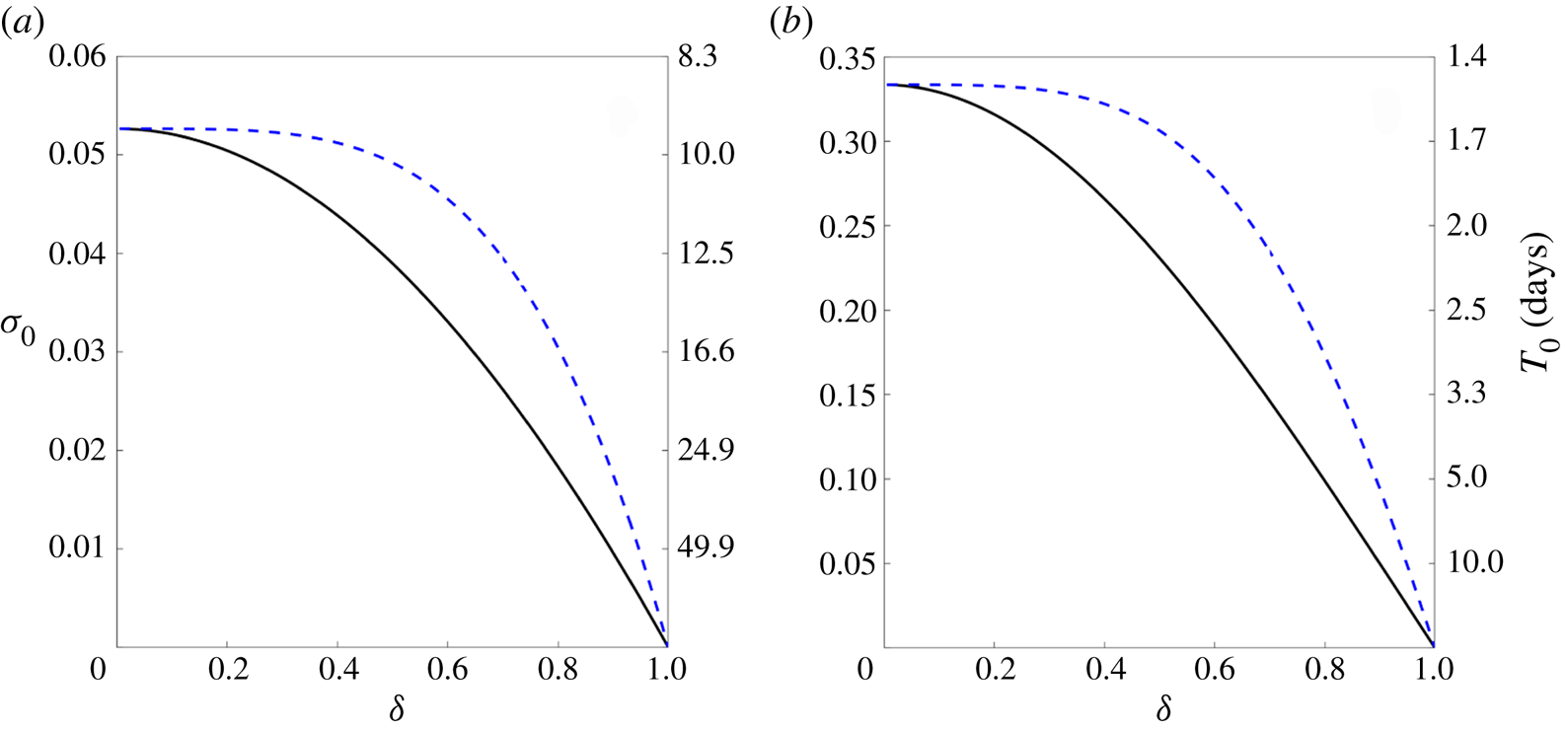
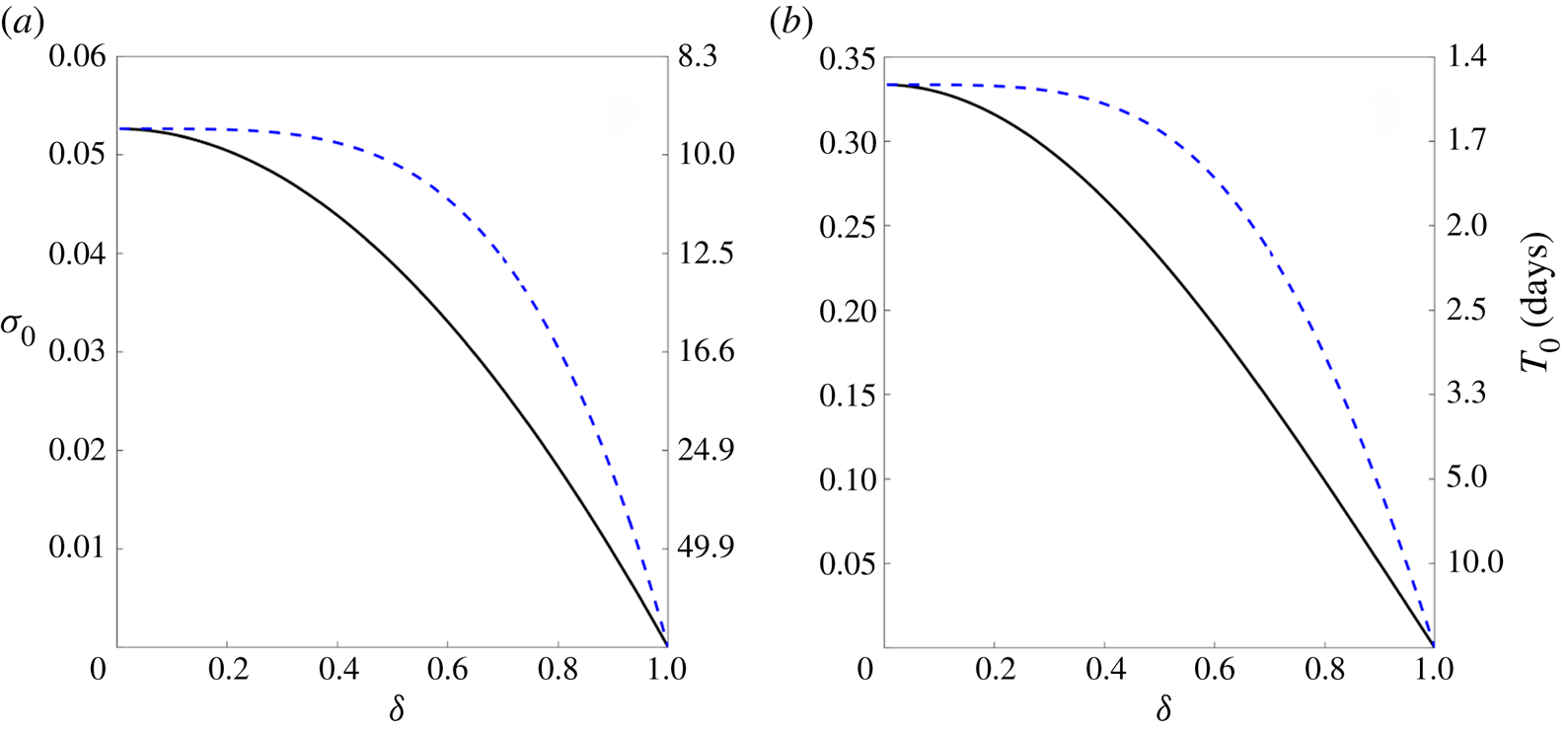
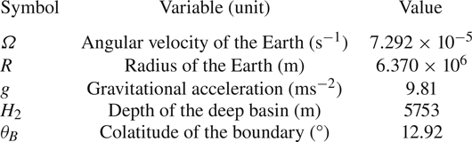
Figure 2 shows a plot of  $\sigma _0$ as a function of
 $\delta$ when
 $m=1$ and
 $m=2$ with two sample values of
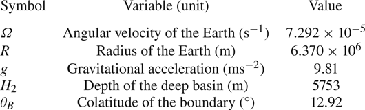
 $\mu$ and using the parameter values listed in table 1. For fixed
 $\mu$ and
 $\delta$ the magnitude of
 $\sigma _0$ decreases with growing
 $m$. As the step height increases so the wave period
 ${\rm \pi} /(\Omega \sigma _0)$ diminishes. For typical Arctic shelves where
 $\mu <0.1$ and
 $0.6\leq \delta \leq 0.9$ the wave period will be of the order of a couple of days.
Leading-order eigenfrequency  $\sigma _0$ as given by (3.10) plotted against
 $\delta$ for modes
 $m=1$ (solid line) and
 $m=2$ (dashed line); (a)
 $\mu =0.9$ and (b)
 $\mu =0.5$. The right-hand axes show the corresponding values of the wave period
 $T_0={\rm \pi} /(\Omega \sigma _0)$ expressed in units of days.
Parameter values adopted for calculations in the paper.
It is worth contrasting our results with their mid-latitude divergent topographic Rossby wave counterparts over a mid-latitude rectilinear step shelf. In this latter case, waves decay exponentially quickly away from the shelf whereas in the present problem the waves decay only algebraically in the deep basin. This difference can be ascribed to the fact that, here, we are dealing with a bounded as opposed to a semi-infinite geometry. Support for this view is provided by the study of Bokhove & Johnson (Reference Bokhove and Johnson1999), who studied waves on a coastal shelf and obtained solutions which decay algebraically away from the shelf break just as we have here. While our investigation shares some similarities with Bokhove & Johnson (Reference Bokhove and Johnson1999), that paper dealt with hybrid Rossby–shelf waves in a cylindrical ocean on a mid-latitude  ${\rm beta}$-plane with a rigid lid, by way of contrast, we have here a polar basin with a free surface. We also remark that there are an infinite number of azimuthal modes which distinguishes it from the unbounded rectilinear problem for which only one shelf wave mode is possible (LeBlond & Mysak Reference LeBlond and Mysak1978).
3.2. First correction
We can deduce the frequency correction term  $\sigma _1$ by proceeding to the next order in the equations. It is helpful to define auxiliary constants
 $P$ and
 $Q^{\alpha }$ according to
 \begin{equation} P\equiv \frac 13-\frac{2}{1-\sigma_0^{2}},\quad Q^{\alpha}=\frac{m^{2}}{3}+\frac{m}{\sigma_0}\left( \frac{1+\sigma_0^{2}}{1-\sigma_0^{2}}\right) +\left( \frac{R}{r_e^{\alpha}}\right)^{2}(1-\sigma_0^{2}), \end{equation}
where  $\alpha =D$ or
 $S$ depending on whether our solution relates to the deep basin or shelf region. With these constant values it follows from
 ${O}(\varepsilon ^{2})$ terms in (3.3) that
 \begin{equation} F_1^{D}=\frac{mP+Q^{D}}{4(m+1)}{X^{m+2}} \end{equation}
and
 \begin{equation} F_1^{S}=B_1X^{m}+C_1X^{-m}+ \frac{B_0(mP+Q^{S})}{4(m+1)}X^{m+2}+\frac{C_0(mP-Q^{S})}{4(m-1)}{X^{2-m}} \end{equation}
provided that  $m\not =1$. The constants
 $B_1$ and
 $C_1$ can be determined by enforcing the two conditions at the step
 $X=\delta$, namely
 \begin{equation} [F_1]^{\delta+}_{\delta-}=0 \end{equation}
and
 \begin{equation} \mu\sigma_0F_{1X}^{S} -\sigma_0F_{1X}^{D} - m\delta^{-1} (\mu F_1^{S}-F_1^{D})= \sigma_1(F_{0X}^{D}-\mu F_{0X}^{S})+\frac{1}{3}m\delta(F_0^{D}-\mu F_0^{S}), \end{equation}
where the subscripts  $X$ denote derivatives. Due to their complexity, the expressions for
 $B_1$ and
 $C_1$ are relegated to appendix A. Then the frequency correction
 $\sigma _1$ is determined by demanding that the edge condition (3.4b) be satisfied at
 $O(\varepsilon ^{2})$:
 \begin{equation} \sigma_0 F_{1X}^{S}-m F_1^{S}=-\sigma_1 F_{0X}^{S} -\frac{1}{3}m F_0^{S}. \end{equation}
This leads to the closed form expression for  $\sigma _1$ in the form
 \begin{align} \sigma_1&= 1-\frac 2\gamma-\frac{\delta^{2}(m+2)}{2(m+1)}+\frac{\delta^{2}}{\gamma(m+1)} -\frac{2}{3\gamma^{2}}(\delta^{2}-3)(\mu+1)-\frac{\mu(\delta^{2}-1)}{1-\gamma}-\frac{\delta^{2}} {3\gamma}\nonumber\\ &\quad -\frac{2\beta(\mu-1)^{2}(\delta^{2m}-1)\delta^{2m}}{\gamma^{3}\mu m(m+1)}+\Phi_m\frac{\mu-1}{\gamma}\left(\frac{m}{\gamma-2}- \frac{4\beta(\gamma-1)^{2}}{\gamma^{3}\mu}\right), \end{align}
in which we have defined
 \begin{equation} \gamma\equiv 1+\mu+(1-\mu)\delta^{2m},\quad \beta\equiv\left(\frac{R}{r_e^{D}}\right)^{2}\quad\textrm{and} \quad\Phi_m\equiv\frac{\delta^{2m}-\delta^{2}}{m^{2}-1}. \end{equation}
In deriving (3.15) we have invoked the result  $r_e^{S}=\sqrt {\mu }r_e^{D}$ to eliminate
 $r_e^{S}$ in favour of
 $r_e^{D}$ although, of course, it is equally possible to express the result in terms of
 $r_e^{S}$.
As  $\delta \to 0$, corresponding to the diameter of the deep basin shrinking, both
 $\sigma _0$ and
 $\sigma _1$ vanish. On the other hand, as the shelf width tends to zero (i.e.
 $\delta \to 1$) we see from (3.15) that
 \begin{equation} \sigma_1= - \frac{2m(1-\mu)+5-2\mu}{6(m+1)}. \end{equation}
Although the shelf wave modes are filtered out in this limit, the planetary wave modes are retained at  $O(\epsilon ^{2})$, the scaling of which agrees with Bassom & Willmott (Reference Bassom and Willmott2019). However, the value of
 $\sigma _1$ in this limit differs from the planetary wave eigenfrequencies derived by Bassom & Willmott (Reference Bassom and Willmott2019). This disagreement is reconciled by noting that as the shelf width tends to zero we require a boundary layer adjacent to the basin boundary such that
 $\delta = 1-D\varepsilon ^{2}$, where
 $D\approx O(1)$. As
 $D\to 0$ the amplitude equation takes the form of a Bessel's equation because when
 $\sigma \approx O(\varepsilon ^{2})$ the first term in the parenthesis of the coefficient of
 $F$ in (2.4) is retained. Exiting this boundary layer (i.e.
 $D\to \infty$), the amplitude equation takes an Euler form because
 $\sigma \approx O(1)$. Within this boundary layer there is no new behaviour of the eigenfunctions. Its role is simply to match the planetary wave eigenfrequencies above with those described in Bassom & Willmott (Reference Bassom and Willmott2019).
3.2.1. The case  $m=1$

When  $m=1$ the above results require some slight modification as it is evident that result (3.12) must be adapted. While the zeroth-order results continue to hold, the first-order eigenfunctions become
 \begin{equation} F_1^{D}=\frac 18(P+Q^{D})X^{3} \end{equation}
and
 \begin{equation} F_1^{S}=B_1X+C_1X^{-1}+ \frac 18B_0(P+Q^{S})X^{3}-\frac 12C_0(P-Q^{S})X\left[ \ln X-\frac 12\right]. \end{equation}
The form of  $\sigma _1$ is obtained by putting
 $m=1$ in expression (3.15) together with the result that
 $\lim _{m\to 1}\Phi _m=\delta ^{2}\ln \delta$ whence
 \begin{align} \sigma_1|_{m=1}&= 1-\frac 2\gamma-\frac 34\delta^{2}+\frac{\delta^{2}}{2\gamma} -\frac{2}{3\gamma^{2}}(\delta^{2}-3)(\mu+1)-\frac{\mu(\delta^{2}-1)}{1-\gamma}-\frac{\delta^{2}} {3\gamma}\nonumber\\ &\quad -\frac{\beta(\mu-1)^{2}(\delta^{2}-1)\delta^{2}}{\gamma^{3}\mu }+\delta^{2}\ln\delta\frac{\mu-1}{\gamma}\left(\frac{1}{\gamma-2}-\frac{4\beta(\gamma-1)^{2}}{\gamma^{3}\mu} \right). \end{align}
4. Results and discussion
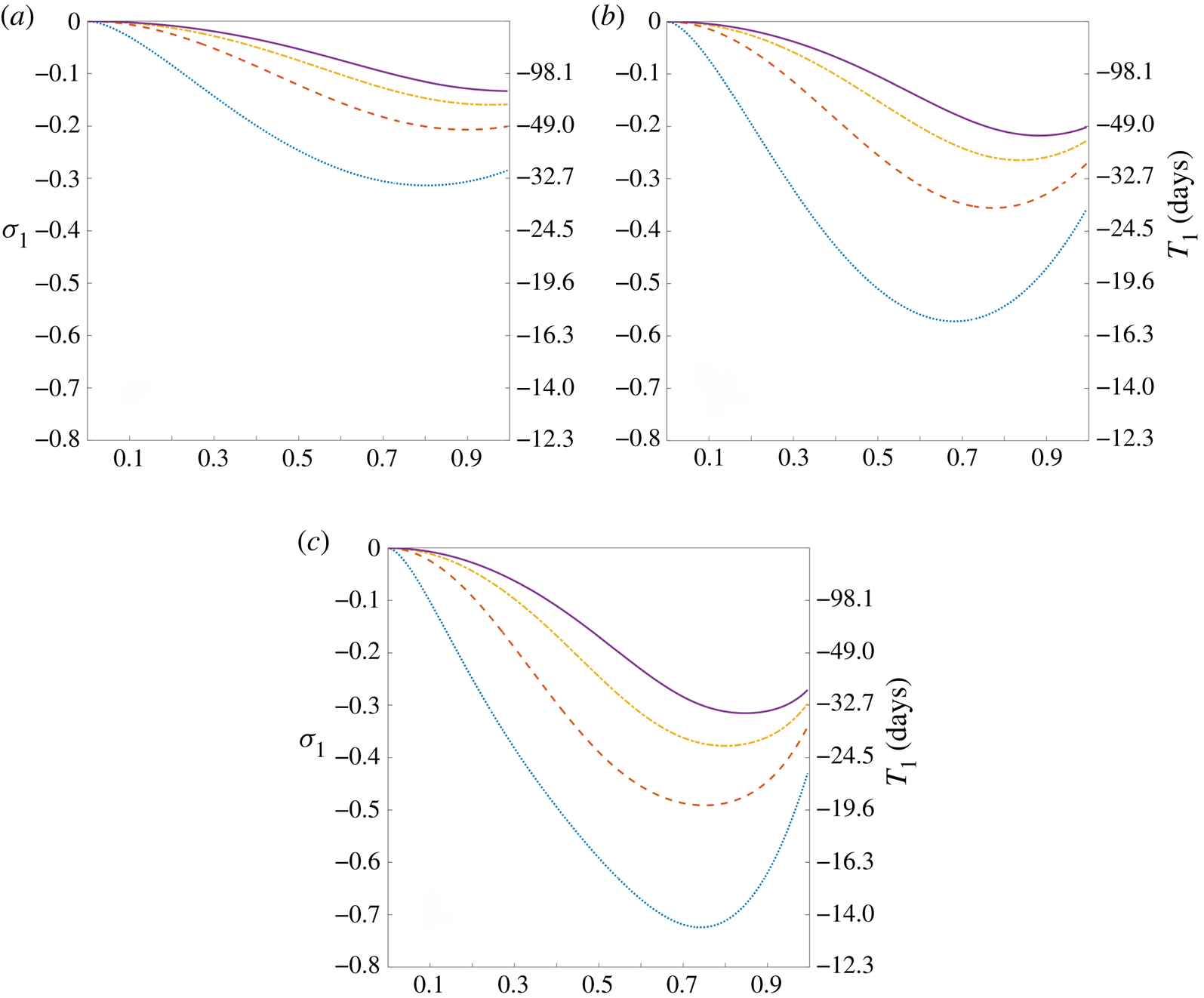
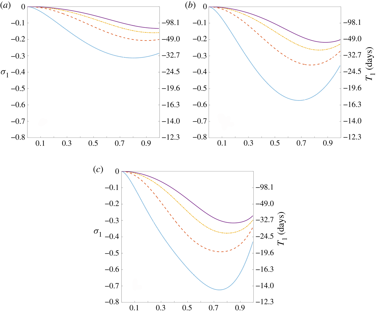
Figure 3 illustrates the form of the frequency correction  $\sigma _1$ as a function of the location of the depth discontinuity at
 $X=\delta$. The sign of
 $\sigma _1$ is negative across the entire
 $\mu -\delta$ parameter space and corresponds to a clockwise propagating planetary wave correction to the value of
 $\sigma _0$. The gravest (i.e.
 $m=1$) mode has period shorter than higher azimuthal modes and as the step height increases its value, is only of the order of a few days. On this time scale one would expect that meteorological forcing could excite this mode. Travelling storms are not uncommon in the Arctic and could generate a near resonant shelf wave response if they propagate anticlockwise around the basin. On the other hand, if the storm travels clockwise around the basin this might lead to a near resonant planetary wave response. In this latter case, the scaling used in this model would not be valid because selected forced planetary wave modes would be more energetic than the shelf wave modes. The planetary wave periods span some tens of days and could perhaps account for the waves observed in the Beaufort Gyre by Timmermans et al. (Reference Timmermans, Rainville, Thomas and Proshutinsky2010) and Zhao & Timmermans (Reference Zhao and Timmermans2018). As the step height decreases, corresponding to
 $\mu \to 1$, the magnitude of the planetary wave frequencies decrease. When
 $\mu =1$, corresponding to the complete absence of topography, the Rossby wave frequency
 $\sigma _0$ and its higher-order corrections vanish.
The frequency  $\sigma _1$ as given by (3.15) for
 $m\not =1$ (and by (3.19) when
 $m=1$) plotted against
 $\delta$. The three plots correspond to the three values (a)
 $\mu =0.9$, (b)
 $\mu = 0.7$ and (c)
 $\mu = 0.5$. In each case the results for the first four modes
 $m\in [1,4]$ are shown with the curves illustrated corresponding to increasing
 $m$ as we move up each graph. The right-hand axes show the corresponding values of the wave period
 $T_1={\rm \pi} /(\varepsilon ^{2}\Omega \sigma _1)$ expressed in units of days.
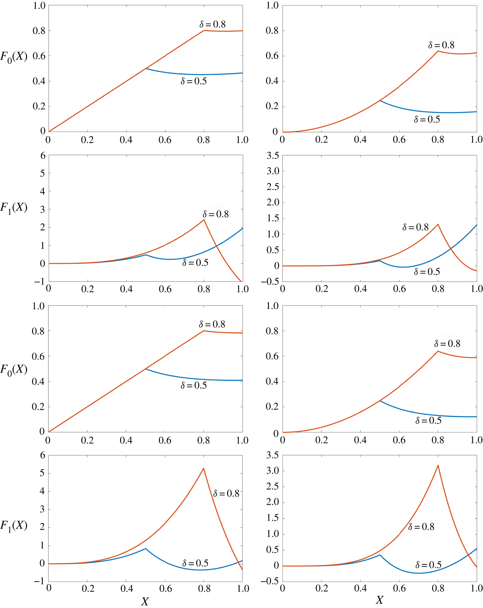
The eigenfunctions  $F_0$ and
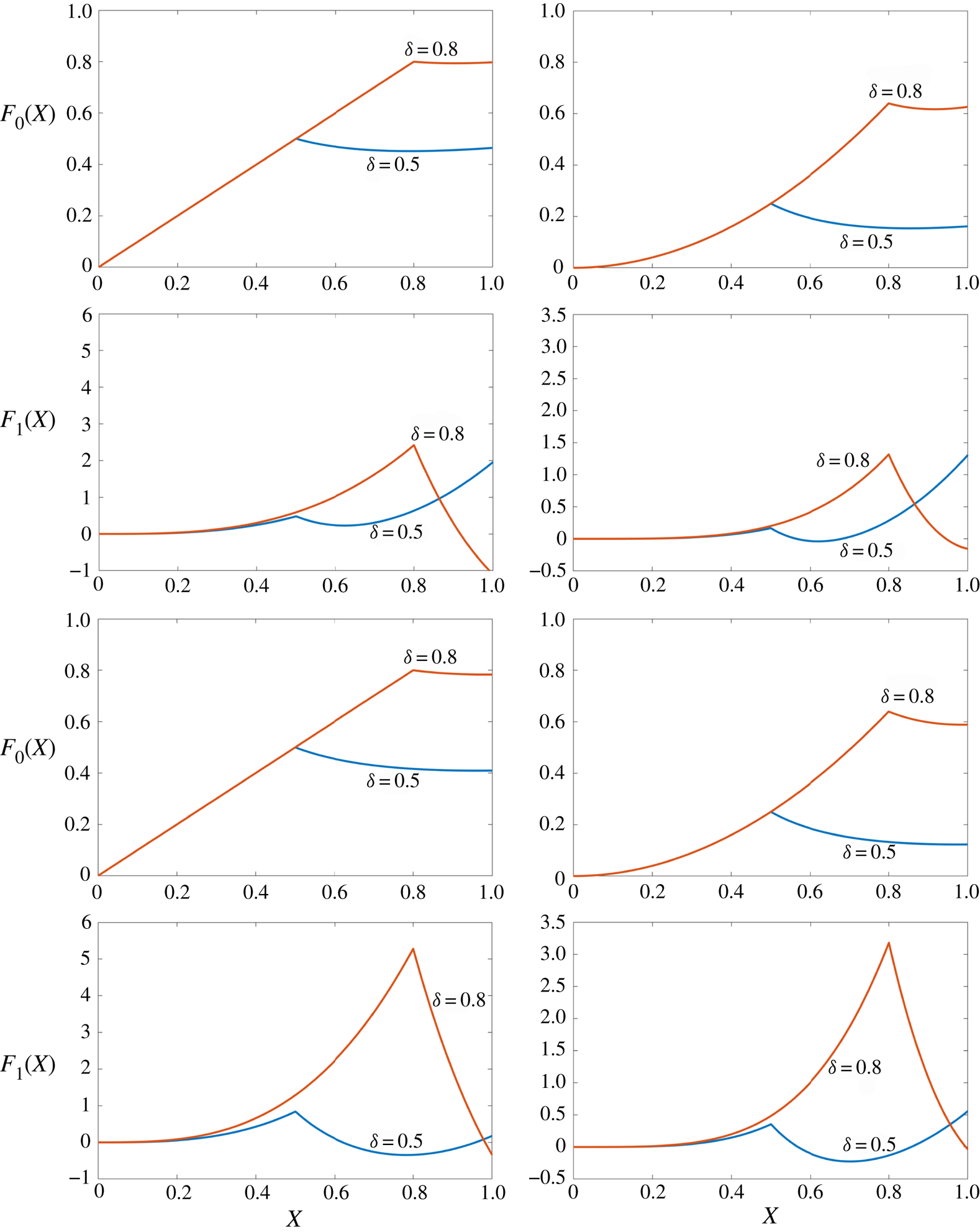
 $F_1$ are plotted in figure 4 for
 $m=1$ and
 $m=2$ and for a selection of parameter values
 $\mu$ and
 $\delta$. As
 $\delta \to 1$ the relative magnitude of the planetary wave eigenfunction
 $F_1$ increases and its maximum value occurs at the shelf break. The combined limits of
 $\delta \to 1$ and
 $\mu \to 1$, leading to a narrow width small amplitude continental shelf, leads to an increase in the amplitude of
 $F_1$ which occurs at the shelf break. This behaviour reflects the fact that as the step height decreases the planetary vorticity gradient associated with topography is reduced while the gradient associated with variation of the Coriolis parameter with colatitude is essentially unchanged. Over a wider shelf (e.g.
 $\delta =0.5$) the planetary wave eigenfunction attains local maxima both at the coast and at the shelf break. As the shelf break height increases so
 $F_1$ exhibits a global maximum at the coast. Locations where the eigenfunctions are largest in absolute value will correspond to where the horizontal currents associated with these modes are greatest.
Plots of the leading-order eigenfunction  $F_0$ as given by (3.7) and (3.8) and the first-order eigenfunction
 $F_1$ as defined by (3.12) for the two step locations
 $\delta =0.5$ and
 $\delta =0.8$. The upper four panels correspond to
 $\mu =0.5$ while the lower four panels have
 $\mu =0.9$; functions in the left-hand column relate to the first mode
 $m=1$ while those in the right-hand column have
 $m=2$.
In our bounded polar basin the decay of the amplitude of the shelf wave modes from the shelf break and the basin boundary is algebraic with radial distance. This contrasts with the exponential decay with cross-shelf distance that is associated with unbounded mid-latitude continental shelves. Thus, over Arctic shelves and in the deep basins the signature of topographic Rossby waves might be more readily observed in time series data of temperature and horizontal currents compared with mid-latitudes. Although Timmermans et al. (Reference Timmermans, Rainville, Thomas and Proshutinsky2010) and Zhao & Timmermans (Reference Zhao and Timmermans2018) observe sub-inertial waves in the Beaufort Gyre, they were unable to comment on their direction of propagation. Both of these studies interpret the wave dynamics in terms of bottom trapped Rossby waves over a small amplitude linear sloping bottom in the presence of a continuously stratified ocean following the theory of Rhines (Reference Rhines1970). The geometry of the deep basin and its location near the pole were not taken into account by Timmermans et al. (Reference Timmermans, Rainville, Thomas and Proshutinsky2010) and Zhao & Timmermans (Reference Zhao and Timmermans2018), which may call into question their interpretation of the waves. Our tentative speculation is that the step-shelf wave guide in a polar cap considered in this paper might be a more appropriate framework for future analysis and interpretation of the hydrographic and current meter data in the Beaufort Gyre.
Stratification has not been considered in this study and its inclusion would be a worthwhile extension for application to the Arctic. In the Beaufort Gyre the deep ocean is almost stratification free, although the upper couple of hundred metres of the water column is strongly stratified where the top of the continental shelf is located. We therefore anticipate that stratification could well modify the wave topographic Rossby wave frequencies in a non-trivial manner.
Acknowledgments
The referees are thanked for their constructive comments. We are grateful to Dr S. Walters for his programming assistance and plotting the figures. A.J.W. thanks the University of Tasmania for the award of a Senior Research Fellowship which supported this project. He also acknowledges the hospitality of the members of the Departments of Mathematics and Physics at the University of Tasmania during a visit in October–November 2019.
Declaration of interests
The authors report no conflict of interest.
Appendix A
Here, for completeness, we record the expressions for the constants  $B_1$ and
 $C_1$ that appear in the solution (3.12b) for
 $F_1^{S}$. It may be shown that
 \begin{equation} \left.\begin{aligned} B_1 & =\frac{\delta}{2\mu m\sigma_0} \{\mu m \delta^{-m-1} (1+\sigma_0) R_1 -\delta^{-m} R_2\},\\ C_1 & =\frac{\delta}{2\mu m\sigma_0} \{-\mu m \delta^{m-1} (1-\sigma_0) R_1 + \delta^{m} R_2\}, \end{aligned}\right\} \end{equation}
in which the auxiliary variables  $R_1$ and
 $R_2$ are in turn given by
 \begin{equation} R_1= \frac{(mP+Q^{D})}{4(m+1)}\delta^{m+2} - B\frac{(mP+Q^{S})}{4(m+1)}\delta^{m+2} -C\frac{mP-Q^{S}}{4(m-1)}\delta^{-m+2} \end{equation}
and
 \begin{align} R_2&= -\frac{1}{3}m\delta^{m+1} (1-mu) - m\sigma_1 \delta^{-1} [\delta^{m}-\mu(B\delta^{m}-C\delta^{-m})]\nonumber\\ &\quad + \frac{\mu B(mP+Q^{S})}{4(m+1)} \delta^{m+1} [2\sigma_0-m(1-\sigma_0)]\nonumber\\ &\quad + \frac{\mu C(mP-Q^{S})}{4(m-1)}\delta^{-m+1}[2\sigma_0-m(1+\sigma_0)]\nonumber\\ &\quad -\frac{mP+Q^{D}}{4(m+1)} \delta^{m+1} [2\sigma_0-m(1-\sigma_0)]. \end{align}