1. Introduction
The Richtmyer–Meshkov instability (RMI) occurs at the rippled surface of separation between two fluids when a planar shock wave comes from one side and hits the contact surface (Richtmyer Reference Richtmyer1960; Meshkov Reference Meshkov1969; Mikaelian Reference Mikaelian1991; Wouchuk & Nishihara Reference Wouchuk and Nishihara1996). This instability has been extensively studied together with its counterpart, the Rayleigh Taylor instability (RTI) due to their influence on the success of inertial confinement fusion (ICF) implosions (Ye Zhou Reference Zhou2017). After the incident shock refraction, two wave fronts are generated, one at each side of the material surface. A shock is always transmitted but, depending on the thermodynamic properties of both fluids, another shock or a centred rarefaction wave may be reflected back (Yang, Zhang & Sharp Reference Yang, Zhang and Sharp1994). The reflected and transmitted wavefronts are also corrugated and, due to the conservation of tangential momentum at the wavefronts, an initial velocity circulation is created on the material surface. The spatially modulated tangential velocity at the ripple induces a pressure gradient along that surface which is responsible for the initial ripple acceleration. As the wavefronts propagate inside both fluids and their ripples oscillate in a damped fashion, a sound wave field is radiated towards the contact surface, which in turn modifies the velocity field near the surface ripple. As a result, the material interface corrugation grows in time and its normal velocity increases. For very small values of the corrugation amplitude compared with the perturbation wavelength, the surface ripple normal velocity usually reaches an asymptotic value (which will be also called the terminal velocity), after some gentle oscillations (Richtmyer Reference Richtmyer1960; Meshkov Reference Meshkov1969; Fraley Reference Fraley1986; Mikaelian Reference Mikaelian1991; Yang et al. Reference Yang, Zhang and Sharp1994; Velikovich et al. Reference Velikovich, Dahlburg, Schmitt, Gardner, Phillips, Cochran, Chong, Dimonte and Metzler2000; Wouchuk Reference Wouchuk2001a
, Reference Wouchuk2001b
). Later, as the surface ripple amplitude becomes comparable to the perturbation wavelength (Vandenboomgaerde et al. Reference Vandenboomgaerde, Souffland, Mariani, Biamino, Jourdan and Houas2014), the instability enters the nonlinear regime and the growth velocity decreases in time due to nonlinear effects. The RMI instability growth in linear theory has been studied in the past for both cases in which a shock (Richtmyer Reference Richtmyer1960; Fraley Reference Fraley1986; Yang et al. Reference Yang, Zhang and Sharp1994) or a rarefaction is reflected at the contact surface (Yang et al. Reference Yang, Zhang and Sharp1994; Velikovich Reference Velikovich1996). The RMI is an important phenomenon in ICF, because thermonuclear targets are never perfectly spherical and/or laser irradiation is non-uniform in general. To reach ignition conditions, an ICF target must be compressed in such a way that a central hot spot forms in the centre at the end of the implosion process. Let us briefly review the conditions for a successful implosion leading to high energy gain. The main objective is to form a central spot with high enough temperatures (
 ${\sim}15\, {\rm keV}$
) in order to initiate fusion reactions. This central hot spot must be surrounded by colder fuel with its density properly shaped in space in such a way that that the alpha particles emitted from the centre will be absorbed by the surrounding, colder fuel, thereby increasing its temperature to finally ignite the whole fuel. Details may be found in Piriz and Wouchuk (Reference Piriz and Wouchuk1992), Lindl et al. (Reference Lindl2014) and references therein. In order to reach these conditions of ignition, symmetry of the implosion is crucial. If the implosion proceeds non-uniformly, the central hot spot will not be formed and the energy gain will be drastically reduced. The irradiation of the outer surface is usually accomplished by means of an irradiation prepulse, followed by the main pulse, or even more complicated shapes. This sequence is necessary in order to shape the entropy of the fuel adequately creating a spot surrounded by colder fuel with properly shaped density in space. The main pulse is needed to later heat the central spot such that it reaches the temperatures needed for self-ignition. For more specific details, the reader is referred to Piriz and Wouchuk (Reference Piriz and Wouchuk1992), Lindl et al. (Reference Lindl2014) and references therein. Typically, the spherical target is composed of several layers of different materials. Usually, the boundaries between the successive layers are not perfectly spherical, because of inherent non-uniformities during target manufacturing (Velikovich et al. Reference Velikovich2020). This characteristic create a serious problem as to the uniformity of the implosion: when the first shock crosses any of the boundaries between successive layers, it may trigger the RMI at each material interface. The RMI growth will then ensue, which might rapidly enter its nonlinear phase. Things worsen immediately upon arrival of the second stronger shock (generated by the main pulse). This second wave will reshock the already existing hydrodynamic perturbations thereby increasing the rate at which the materials on each side of the interface mix with each other. As for the physics of re-shock, the interested reader is referred to the numerical study of Latini et al. (Reference Latini2007) and the recent experimental work of Cao et al. (Reference Cao2024) The overall picture worsens when taking into account that at each material surface there will be a whole spectrum of initial corrugations, which, after entering the nonlinear stage of growth, might become turbulent, seriously damaging target uniformity. Even worse is the fact that these hydrodynamic perturbations will serve as seeds for the later, more deleterious RTI, which may disrupt the target (RTI growth is exponential in time); see Ye Zhou (Reference Zhou2017). A legitimate and totally justified question then arises: In which way could theoretical models like the one presented here help in the design of ICF experiments in order to mitigate instability growth as much as possible?
To answer this important question, it is convenient to recall another aspect of the RMI that may be of help. In Mikaelian (Reference Mikaelian1991) predicted the possibility of stopping the growth of the RMI thanks to freeze-out. This phenomenon was later confirmed in Wouchuk & Nishihara (Reference Wouchuk and Nishihara2004) for the shock reflected case by means of the compressible linear theory developed in Wouchuk (Reference Wouchuk2001a ), and for the rarefaction reflected case in Wouchuk & Sano (Reference Wouchuk and Sano2015). It is noted that freeze-out is independent of the perturbation wavelength. Hence, if conditions are adequate for freeze-out, none the perturbation wavelengths imprinted on the surface will grow. Therefore, a whole multi-mode spectrum may be frozen out and it will not grow turbulently. Hence, there is the possibility that, if the properties of the materials (densities and isentropic exponents) are conveniently chosen, RMI growth at each boundary might be totally suppressed. The exact calculation of the freeze-out conditions is only possible with full compressible calculations as developed in Wouchuk (Reference Wouchuk2001a ) and Wouchuk & Sano (Reference Wouchuk and Sano2015). Thus, linear calculations like the ones presented here may be useful to benchmark the hydrocodes used in ICF, and assist in the design of more robust thermonuclear targets.
There is still another important pay off for analytic linear compressible models. Nonlinear calculations, like those shown in Matsuoka et al. (Reference Matsuoka2003, Reference Matsuoka2020) and Matsuoka & Nishihara (Reference Matsuoka and Nishihara2023) are usually done once the perturbation velocity field has become incompressible. Still, the calculations of Matsuoka et al. (Reference Matsuoka2003, Reference Matsuoka2020), Matsuoka & Nishihara (Reference Matsuoka and Nishihara2023) need to be initialised with data from the compressible linear stage. Thus, calculations like the ones presented here may be useful to calculate the nonlinear evolution of the RMI in conditions relevant to ICF, and/or help in the design of successful target implosions, whether because they help finding realistic freeze-out conditions, or because they are used to initialise the complicated calculations of nonlinear models like the Vortex Sheet Model of Matsuoka et al. (Reference Matsuoka2020) .
The main purpose of the present work is to derive a tractable, albeit approximate, analytical expression for the terminal velocity that might be useful for studying regimes of high compression and help in the benchmarking of hydrocodes as well as helping develop nonlinear models in regimes of high compression. This work is structured as follows: in § 2 the one-dimensional background (zero-order) profiles upon which the instability evolves are presented, calculating first the reflected and transmitted shock intensity parameters (
 $z_r$
, and
 $z_t$
, respectively). All the background quantities necessary for later calculations are shown as functions of
 $z_r, z_t$
. The linear theory perturbation problem is presented in § 3. The linearised equations of motion are shown in § 4. The necessity and usefulness of the Laplace transform is briefly discussed in § 5. The linearised Rankine Hugoniot equations are shown in § 6. The important functional equations satisfied by the reflected and transmitted shock pressure perturbations are derived in § 7, after discussing the feasibility of a rigid piston approximation (RPA for short). These equations are solved exactly in § 8 using elementary tools of complex calculus in one variable. In § 9, the important method of inverting the Laplace transforms in order to get the temporal evolution of the perturbations is discussed, and explicit analytical formulas are given. The ordinary differential equations satisfied by the components of the asymptotic velocity field are also derived in § 9. The important (1.3) is rederived for easy of discussion.
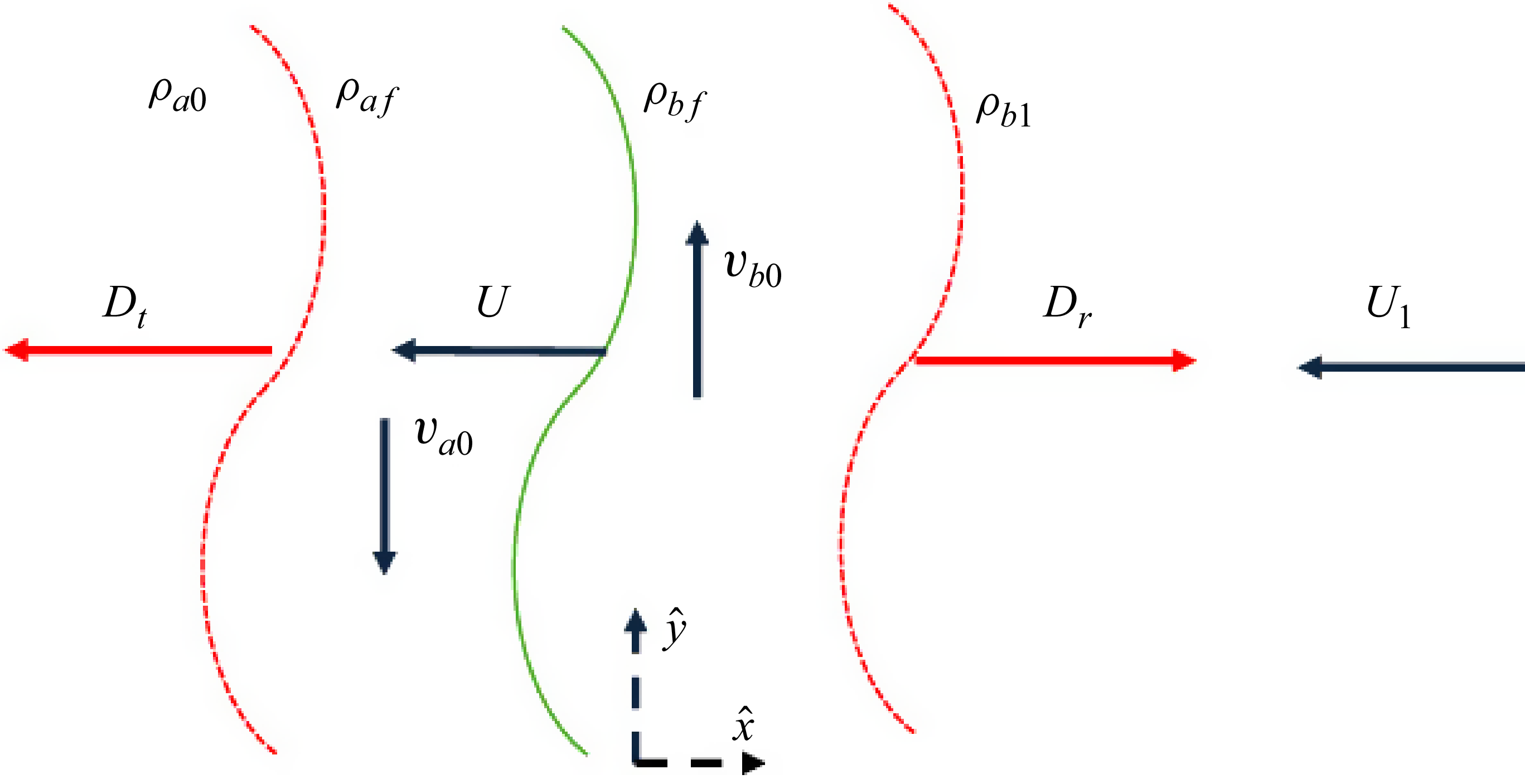
Let us concentrate on figure 1. An incident shock comes from the right, inside fluid ‘b’ with velocity
 $-D_i \hat {x}$
in the laboratory reference frame. The contact surface is initially at rest, and located at
 $x = 0$
. The incident shock hits the contact surface at
 $t = 0$
. Each fluid is assumed to be an ideal gas with specific heat ratios
 $\gamma _a$
and
 $\gamma _b$
, respectively. The densities of each fluid, before shock compression, are given by
 $\rho _{a0}$
and
 $\rho _{b0}$
, respectively. We define here the pre-shock density ratio
 $R_0 = \rho _{a0}/\rho _{b0}$
; see figure 1. We define, following Whitham (Whitham Reference Whitham1973), the incident shock strength parameter
 $z_i = p_1/p_0-1$
, with
 $p_0$
the initial pressure in both fluids and
 $p_1$
the pressure behind the incident shock. If we define the quantity
 $\epsilon _{b1} = {\gamma _b+1}/{2 \gamma _b}$
, the upstream incident shock Mach number is equal to
 \begin{equation} M_i = \frac {D_i}{c_{b0}} = \sqrt {1+\epsilon _{b1} z_i}. \, \end{equation}
Incident shock and contact surface, before shock refraction at
 $t = 0$
, in one-dimensional geometry.
 $U_1$
is the fluid velocity behind the incident shock.

The quantity
 $c_{b0}$
is the initial sound speed of fluid ‘b’ given by
 \begin{equation} c_{b0} = \sqrt {\frac {\gamma _b \ p_0}{\rho _{b0}}} . \end{equation}
The fluid compressed by the incident shock acquires a velocity
 $-U_1 \hat {x}$
in the laboratory frame of reference and its density increases from
 $\rho _{b0}$
to
 $\rho _{b1}$
. The sound speed of the compressed fluid ‘b’ across the incident shock is indicated with
 $c_{b1}$
. After shock refraction, on the side of fluid ‘a’, a transmitted shock propagates to the left with speed
 $D_t$
The pressure behind the transmitted front is
 $p_f$
(the same as the pressure in the space between the reflected shock wave and the contact surface) and the corresponding shock strength is
 $z_t = (p_f-p_0)/p_0$
. The transmitted shock Mach number is thus:
 $M_t = D_t/c_{a0} = \sqrt {1+\epsilon _{a1} z_t}$
, where
 $\epsilon _{a1} = {\gamma _a+1}/{2 \gamma _a}$
. After shock compression, the contact surface acquires a normal velocity, which we indicate with
 $U$
. It is equal to
 $U= c_{a0} z_t/(\gamma _a M_t)$
. We assume a sinusoidal corrugation for the contact surface ripple of the form
 $\psi _0 \cos k y$
, where
 $\lambda$
is the corrugation wavelength and
 $k = 2\pi /\lambda$
is the perturbation wavenumber, and impose the condition:
 $\psi _0 \ll \lambda$
so that a linear theory analysis is warranted. The incident shock refracts in a time scale of the order of
 $ \Delta t_0 \approx 2\psi _0/D_i$
, which is therefore very small. For notational simplicity, we indicate this time as
 $t = 0+$
. Then, at
 $t =0+$
a reflected shock or a rarefaction fan are formed inside fluid ‘b’ and a transmitted shock front is always driven into fluid ‘a’. Whether a shock or a rarefaction is formed inside fluid ‘b’ depends on the incident shock Mach number, the pre-shock density ratio
 $R_0 = \rho _{a0}/\rho _{b0}$
and the isentropic exponents
 $\gamma _a$
, and
 $\gamma _b$
(Yang et al. Reference Yang, Zhang and Sharp1994; Velikovich Reference Velikovich1996). In this work we only consider cases in which a shock is reflected. In figure 1 we show a transmitted and reflected shock. If
 $\gamma _a = \gamma _b$
, a shock is reflected if and only if
 $R_0 = \rho _{a0}/\rho _{b0} \gt 1$
. If
 $R_0 \lt 1$
, a rarefaction will be reflected. However, if
 $\gamma _a \neq \gamma _b$
, the type of front reflected inside fluid ‘b’ would also be dependent on the incident shock strength, as discussed in Yang et al. (Reference Yang, Zhang and Sharp1994), Velikovich (Reference Velikovich1996). In any case, the final density of fluid ‘b’ at the contact surface is indicated here by
 $\rho _{\textit{bf}}$
, its sound speed by
 $c_{\textit{bf}}$
and the pressure on side ‘b’, at the contact surface (
 $x = 0$
), is
 $p_f$
. The final density ratio at the surface is indicated:
 $R = \rho _{\textit{af}}/\rho _{\textit{bf}}$
. It is clear that the final pressure of fluid a between the transmitted shock and the contact surface is also
 $p_f$
.
After
 $t = 0+$
, when both fronts have moved one or several perturbation wavelengths away from
 $x=0$
, the normal perturbation velocity at the surface ripple would have almost reached its asymptotic value, which we call
 $\delta v_{xc}^{\infty }$
(subscript c stands for contact surface). As discussed in Wouchuk (Reference Wouchuk2001a
, Reference Wouchuk2001b
), Wouchuk & Nishihara (Reference Wouchuk and Nishihara1997) and Wouchuk (Reference Wouchuk2025), the asymptotic normal velocity
 $\delta v_{xc}^{\infty }$
at the contact surface ripple is given by the following exact expression, valid for any shock intensity, in linear theory:
 \begin{equation} \delta v_{xc}^{\infty } = \frac {\delta v_{yb}^0 - R \delta v_{ya}^0}{1+ R} +\frac {- \mathcal{F}_b + R \mathcal{F}_a}{R+1} , \end{equation}
where
 $\delta v_{ya}^0$
and
 $\delta v_{yb}^0$
are the values of the tangential velocities generated on each side of the contact surface at
 $t = 0+$
by the corrugated shocks. The quantities
 $\mathcal{ F}_a$
and
 $\mathcal{F}_b$
are particular averages of the pressure perturbations at the corrugated shock fronts inside both fluids. The term
 $\mathcal{F}_a$
is proportional to a temporal average of the transmitted shock pressure perturbations in time (Wouchuk & Nishihara Reference Wouchuk and Nishihara1997; Wouchuk Reference Wouchuk2001a
, Reference Wouchuk2001b
)
 \begin{equation} \mathcal{F}_a \propto \int _{0+}^{\infty } \delta p_t(t) e^{-\beta _t t} {\rm d}t . \end{equation}
The proportionality constant will be derived later to calculate the velocity profiles inside each fluid. In (1.4) above, the quantity
 $\delta p_t$
is the pressure perturbation just behind the transmitted shock front and
 $\beta _t = (D_t-U)/c_{\textit{af}}$
is the transmitted shock Mach number with respect to the compressed fluid a. It will be seen that
 $\mathcal{F}_a$
is negligible for weak shocks (typically, for
 $M_t \ll 1.5$
) but not so for stronger shocks. It is recalled here that
 $\mathcal{F}_a$
can also be interpreted as a weighted spatial average of the vorticity generated by the transmitted front inside fluid
 $a$
, see, for example, Wouchuk (Reference Wouchuk2001a
, Reference Wouchuk2001b
), Wouchuk & Nishihara (Reference Wouchuk and Nishihara1997) and Wouchuk (Reference Wouchuk2025). Similarly with
 $\mathcal{F}_b$
.
2. Zero-order profiles
First, it is convenient to develop the equations that give us the zero-order quantities and hence describe the background upon which the instability evolves. Referring to figure 1, we consider an incident shock coming from the right, inside fluid b, with speed
 $D_i$
in the laboratory frame that hits the contact surface located at
 $x = 0$
, at the instant of time
 $t = 0$
. The pre-shock density of fluid a is
 $\rho _{a0}$
, and we define the pre-shock density ratio at the contact discontinuity:
 $R_0 = \rho _{a0}/\rho _{b0}$
. Following Yang et al. (Reference Yang, Zhang and Sharp1994) we define another intensity parameter
 $s$
for the incident shock
 \begin{equation} s = (p_1-p_0)/p_1 . \end{equation}
However, it is also convenient for us to work with the intensity parameter
 $z_i$
, as defined in Whitham’s book (Whitham Reference Whitham1973)
 \begin{equation} z_i = (p_1-p_0)/p_0 = s/(1-s) . \end{equation}
It is relatively easy to express the different quantities behind the incident shock in terms of
 $z_i$
, but we use
 $s$
when comparing with Yang et al. (Reference Yang, Zhang and Sharp1994).
For later use, it will be necessary to have weak shock expansions of the different zero-order quantities up to order
 $z_i^3$
, We apologise here that, because of space limitations, we cannot show here all the coefficients appearing in the weak shock third-order expansions, and they should be worked out by the interested reader. Because of this constraint, we show, nevertheless, all the expansion coefficients in the Supplementary materials are available at https://doi.org/10.1017/jfm.2025.10740. It is a Mathematica file, and anyone with some experience using Mathematica should be able to work with it. It is advised, however, that the interested reader takes a look at Supplementary materials, before working with the Mathematica files. The author tried to follow the notation of this paper inside the Mathematica files. We proceed here with the incident shock Mach number expansion
 \begin{equation} M_{inc} \sim 1 + m_{i1} z_i + m_{i2} z_i^2 + m_{i3} z_i^3 , \end{equation}
where its coefficients are easy to obtain
 \begin{equation} m_{i1} = \epsilon _{b1}/2 .\end{equation}
Coefficients
 $m_{i2}, m_{i3}$
may be found inside Supplementary materials. The incident shock sets fluid b in motion, with velocity
 $-U_1 \hat {x}$
, in the laboratory frame. The fluid velocity
 $U_1$
is given by
 \begin{equation} \frac {U_1}{c_{b0}} = \frac {z_i}{\gamma _b M_i}. \ \end{equation}
The density compression ratio across the incident shock is
 \begin{equation} R_i = \frac {1+ \epsilon _{b1} z_i}{1 + \epsilon _{b2} z_i} , \end{equation}
where we recall
 $\epsilon _{b1} = {\gamma _b+1}/{2 \gamma _b}$
,
 $\epsilon _{b2} = {\gamma _b-1}/{2 \gamma _b}$
. The sound speed inside fluid b increases from
 $c_{b0}$
to
 $c_{b1}$
, across the incident shock, according to
 \begin{equation} \frac {c_{b1}}{c_{b0}} = \sqrt {\frac {1+z_i}{R_i}} . \end{equation}
We rename, for simplicity:
 $c_{b10} = c_{b1}/c_{b0}$
.
The weak shock expansion of
 $c_{b10}$
can be found inside Supplementary materials.
The downstream shock Mach number of the incident front is
 \begin{equation} \beta _i = \sqrt {\frac {1+ \epsilon _{b2} z_i}{1 + \epsilon _{b1} z_i} }\lt 1 . \end{equation}
At
 $t = 0$
, the incident shock hits the contact surface: a reflected shock goes back inside fluid b and a transmitted shock moves inside fluid a. The pressure in the space between the reflected and transmitted shocks is denoted by
 $p_f$
. Hence, the reflected and transmitted intensity parameters are (see figure 1)
 \begin{align} \begin{split} z_r &= \frac {p_f-p_1}{p_1} , \\ z_t &= \frac {p_f-p_0}{p_0} \end{split}\end{align}
Fluid a between the contact surface and the transmitted shock moves to the left with speed
 $U$
, given by
 \begin{equation} \frac {U}{c_{a0}} =\frac {z_t}{\gamma _a M_t} .\end{equation}
In units of the incident shock speed, it is equal to
 \begin{equation} \frac {U}{D_i} = \frac {z_t}{\theta \ \gamma _a M_t M_i} , \end{equation}
where the dimensionless quantity
 $\theta$
above is defined as
 \begin{equation} \theta = \frac {c_{b0}}{c_{a0}} = \sqrt {\frac {\gamma _b R_0}{\gamma _a}} . \end{equation}
It is noticed that the parameter
 $\theta$
is equal to the reciprocal of Fraley’s parameter
 $y$
(Fraley Reference Fraley1986).
Besides,
 $M_t$
is the upstream transmitted shock Mach number
 \begin{equation} M_t = \frac {D_t}{c_{a0}} = \sqrt {1 +\epsilon _{a1} z_t} \gt 1 . \end{equation}
The upstream reflected shock Mach number is
 \begin{equation} M_r = \frac {D_r}{c_{b1}} = \sqrt {1 +\epsilon _{b1} z_r} \gt 1 . \end{equation}
As will be discussed later, we will need expansions of the background quantities up to order
 $z_i^3$
when analysing the weak shock behaviour of the asymptotic velocity. These expansions are shown in detail inside Supplementary materials.
According to figure 1, fluid
 $b$
between the contact surface and the reflected shock moves to the left with the same speed
 $-U \hat {x}$
as the contact surface. The downstream Mach number of the transmitted shock,
 $\beta _t$
, is given by
 \begin{equation} \beta _t = \frac {D_t- U}{c_{\textit{af}}} = \sqrt {\frac {1 +\epsilon _{a2}z_t}{1+ \epsilon _{a1} z_t}} \lt 1. \end{equation}
Where have defined
 $\epsilon _{a1} = {\gamma _a+1}/{2 \gamma _a},\, \text{and}\,\, \epsilon _{a2} = {\gamma _a-1}/{2 \gamma _a}$
. Correspondingly, the downstream Mach number of the reflected shock is
 \begin{equation} \beta _r = \frac {D_r + U}{c_{\textit{bf}}} = \sqrt {\frac {1+ \epsilon _{b2} z_r}{1+\epsilon _{b1} z_r}} \lt 1. \end{equation}
It is necessary to define here, for later use, the quantity
 $\chi _r$
 \begin{equation} \tanh \chi _r = \beta _r \ \gt 0. \end{equation}
We also define a similar quantity associated with the transmitted shock, called
 $\chi _t$
 \begin{equation} \tanh \chi _t = - \beta _t \lt 0. \end{equation}
The quantity
 $\chi _t$
is negative for reasons that will become clear later on when we solve the linear perturbation problem. We calculate next the density ratios across the reflected and transmitted shocks, respectively,
 \begin{align} R_{\textit{refl}} &= \frac {1+ \epsilon _{b1}z_r}{1+\epsilon _{b2} z_r} \gt 1 , \end{align}
 \begin{align} R_{\textit{tr}}&= \frac {1+\epsilon _{a1} z_t}{1+ \epsilon _{a2} z_t} \gt 1. \end{align}
From these values we easily get the ratio of sound velocities across of the reflected and transmitted shock, respectively,
 \begin{align} \frac {c_{\textit{bf}}}{c_{b1}} &= \sqrt {\frac {1+z_r}{R_{\textit{refl}}}}, \end{align}
 \begin{align} \frac {c_{\textit{af}}}{c_{a0}} &= \sqrt {\frac {1+z_t}{R_{\textit{tr}}}}. \end{align}
The final density ratio at the contact surface is thus
 \begin{equation} R =R_0/(R_i R_{\textit{refl}}) . \end{equation}
It is also convenient to have the ratio of post-shock sound velocities at both sides of the contact surface
 \begin{equation} Q = \frac {c_{\textit{af}}}{c_{\textit{bf}}} = \frac {c_{\textit{af}}}{c_{a0}} \frac {c_{b1}}{c_{\textit{bf}}} \frac {c_{b0}}{c_{b1}} Q_0, \end{equation}
where
 $Q_0$
is its pre-shock value, given by
 \begin{equation} Q_0 = \frac {c_{a0}}{c_{b0}} =\frac {\gamma _a}{\gamma _b} \theta , \end{equation}
with
 $ \theta = \sqrt { {\gamma _b R_0}/{\gamma _a}}$
. The quantity
 $\theta$
was defined previously, and is equal to the reciprocal of the quantity
 $y$
used by Fraley (Reference Fraley1986). The quantity
 $Q$
above is the ratio of post-shock sound speeds at both sides of the contact surface. In our previously published work, we indicated this quantity with the capital letter
 $\mathcal{N}$
, but N is a protected symbol inside Mathematica, and because of this, the letter
 $Q$
is used inside the Mathematica files appended to this article, namely, inside Supplementary materials.
It is clear that to solve for the background quantities of the zero-order problem we need the shock intensities
 $z_r, z_t$
as functions of
 $R_0, \gamma _a, \gamma _b, z_i$
.
To this end, the necessary equations result from asking for continuity of pressure and normal velocity at the contact surface. Translated into the language of the variables
 $z_r$
,
 $z_t$
, these conditions read
 \begin{align} z_t &= z_i + (1+ z_i) z_r , \end{align}
 \begin{align} \frac {z_i}{ M_i} - \frac {c_{b1}}{c_{b0}} \frac {z_r}{ M_r} &= \theta \frac {z_t}{M_t} , \end{align}
where
 $ \theta = ({\gamma _b}/{\gamma _a})({c_{a0}}/{c_{b0}}) $
.
It is very difficult to obtain an explicit analytical solution for
 $z_r, z_t$
from the above system of equations. However, scientific software like Mathematica usually gives very accurate estimates of
 $z_r, z_t$
.
For later use, we will need the weak shock scaling of the quantities
 $e^{\pm \chi _r}, e^{\pm \chi _t}$
. We start with
 $e^{-\chi _r}$
: from (2.17), we easily get
 \begin{equation} e^{-\chi _r} = \sqrt {\frac {1- \beta _r}{1+ \beta _r}} . \end{equation}
If we expand
 $z_r$
and
 $\beta _r$
in powers of
 $z_i$
, for
 $z_i \ll 1$
we soon arrive at the lowest possible order in
 $z_i$
 \begin{align} e^{+\chi _r} &\sim \frac {1}{\sqrt {z_i}} , \end{align}
 \begin{align} e^{-\chi _r}&\sim \sqrt {z_i} . \end{align}
Similar scalings hold for
 $e^{\pm \chi _t}$
.
3. Linear perturbation theory
In this section we start considering the situation in which the incident shock hits a corrugated contact surface. We assume an initial corrugation imprinted on the contact surface which depends on the tangential coordinate
 $y$
in the form:
 $\psi _c(t=0, y) = \psi _0 \cos k y$
, where
 $k = 2 \pi /\lambda$
is the corrugation wavenumber. The corrugation wavelength
 $\lambda$
is much larger than the initial ripple amplitude:
 $\psi _0 \ll \lambda$
so as to ensure the validity of a linear theory. In figure 2 we show the typical geometry after the incident shock refraction (
 $t = 0+$
). Because the contact surface is rippled, the reflected and transmitted wavefronts will be as well. Let
 $\psi _r(t) \cos k y$
and
 $\psi _t(t) \cos k y$
be the reflected and transmitted ripple amplitudes, respectively. As is well known, both amplitudes oscillate in a damped fashion, while the shocks separate away from the contact surface. At the same time, pressure perturbations irradiated by the corrugated shocks arrive at the contact surface, get refracted there and continue to catch the shock on the other side of the contact surface. It is noticed here that, because the shocks move with respect to the contact surface, the Doppler effect will be an important mechanism governing the dynamics of the acoustic pressure field. The Doppler effect will have a profound influence in the algebra of the pressure perturbation fields. Since the works of Richtmyer (Reference Richtmyer1960) and Meshkov (Reference Meshkov1969), it is known that the amplitude of the contact surface ripple reaches a constant velocity of growth (the terminal velocity) when
 $t \rightarrow \infty$
, that is, when the refracted shocks are very far from the contact surface (equivalently, for values of the time
 $t$
such that:
 $(D_r + U) t \gg \lambda$
,
 $(D_t - U)\ t \gg \lambda$
).
Initial tangential velocities at both sides of the contact surface, after shock refraction at
 $t = 0+$
; two-dimensional geometry.

Before proceeding to solve the fluid equations in the space between the reflected and transmitted shock, it is convenient to briefly discuss here the origin of the fluid perturbations in both fluids. As is well known (Landau & Lifshitz Reference Landau and Lifshitz1986), across the surface of a shock wave, tangential velocity is conserved, and it is this mechanism that lies at the heart of the pressure and velocity perturbation fields’ evolution in both fluids, as will become evident later.
Even though the incident shock is planar for
 $t\lt 0$
, the reflected and transmitted fronts are not, they are corrugated and the initial amplitudes of their ripples are given below.
The initial amplitude of the ripple at the transmitted front is (Richtmyer Reference Richtmyer1960)
 \begin{equation} \psi _{t0} = \left ( 1- \frac {D_t}{D_i} \right ) \psi _0 , \end{equation}
and the initial amplitude of the reflected shock ripple is
 \begin{equation} \psi _{r0} = \left ( 1 + \frac {D_r}{D_i}\right ) \psi _0 . \end{equation}
As commented before, the tangential velocity is conserved across each rippled front (Landau & Lifshitz Reference Landau and Lifshitz1986) This fact allows us to calculate the dimensionless velocities
 $v_{a0}$
and
 $v_{b0}$
The tangential velocity behind the reflected and transmitted front are, respectively,
 $\delta v_{yb0} = (U_1- U) k \ \psi _{r0}$
,
 $\delta v_{ya0} = - U k \quad \psi _{t0}$
Below, we express both velocities in units of
 $D_i$
 \begin{align} v_{b0} &=\frac {\delta _{vyb0}}{D_i} = \left ( \frac {U_1}{D_i} - \frac {U}{D_i} \right ) k \ \psi _{r0} , \end{align}
 \begin{align} v_{a0} &= \frac {\delta v_{ya0}}{D_i} = - \frac {U}{D_i} k \ \psi _{t0} . \end{align}
Once the corrugated reflected and transmitted shocks start moving inside their respective fluids, the ripple amplitudes start oscillating and decay in a somewhat damped fashion. This process generates pressure fluctuations behind each front that fill the space in between. These pressure perturbations are responsible of accelerating the fluid particles and hence are responsible of the asymptotic motion of the ripple at the contact surface. Besides, as we will see below, the conservation of tangential velocity at each corrugated front is also responsible of creating vorticity in the compressed fluids. As will be clear later on, the calculation of the vorticity field stored in each fluid is necessary in order to determine the value of the terminal velocity. The weak shock expansions of
 $R$
, and
 $v_{a0},\ v_{b0}$
are shown inside Supplementary materials.
4. Linearised fluid equations
We start defining the dimensionless quantities of interest in our work. We recall that we work in a system of reference that moves with velocity
 $U$
, the velocity of compressed fluid a. First, in order to compare with the results of Yang et al. (Reference Yang, Zhang and Sharp1994), we express all the perturbation velocities in units of the incident shock speed. Besides, given that we are solving a linear theory problem, all the perturbed quantities of interest are proportional to
 $k \psi _0$
. Hence, we adopt the definitions that follow below. The pressure perturbations inside fluid
 $m$
are normalised in units of
 $\rho _{\textit{mf}} c_{\textit{mf}} D_i \ k \psi _0$
 \begin{align} \delta v_x(x, y, t) &= u(x, t) \ D_i \cos k y \ k \psi _0 , \nonumber \\ \delta v_y(x,y,t) &= v(x,t) \ D_i \sin k y \ k \psi _0 , \nonumber \\ \delta p_m(x, y, t) &= \rho _{\textit{mf}} c_{\textit{mf}} \ D_i \ \hat {p}_m(x,t) \cos k y \ k \psi _0 , \end{align}
 \begin{align} \delta \rho _m &= \rho _{\textit{mf}} \hat {\rho }_m k \psi _0. \\[9pt] \nonumber \end{align}
We consider inviscid, ideal gases. The linearised, non-dimensional equations of motion inside fluid
 $m = a, b$
(we define the dimensionless time
 $(\tau _m = k c_{\textit{mf}} t$
), are
 \begin{align}\begin{split} \frac {\partial u_m(x, \tau _m)}{\partial \tau _m} &= -\frac {\partial \hat {p}_m}{\partial k x} , \\ \frac {\partial v_m}{\partial \tau _m} &= \hat {p}_m , \\ \frac {\partial \hat {p}_m}{\partial \tau } &= \frac {\partial \hat {\rho }_m}{\partial \tau } . \end{split}\end{align}
The previous equations correspond to the conservation of longitudinal and tangential momentum and energy, respectively. The energy conservation for inviscid fluids is equivalent to the conservation of entropy of the fluid particles (Landau & Lifshitz Reference Landau and Lifshitz1986). As has been extensively used in previous works, it is convenient to change to the variables
 $r, \chi$
, inside each fluid, defined by Briscoe & Kovitz (Reference Briscoe and Kovitz1968) and Zaidel (Reference Zaidel’1960) as
 \begin{align} k x &= r \sinh \chi , \end{align}
 \begin{align} \tau _m &= r \cosh \chi . \end{align}
It is easy to see that, inside fluid
 $b$
, the compressed fluid occupies the region between
 $\chi = 0$
and
 $\chi = \chi _r = \tanh ^{-1} \beta _r$
. The transmitted shock, on the other hand, moves inside fluid
 $a$
with negative velocity, and hence, compressed fluid
 $a$
occupies the region between
 $\chi = \chi _t = -\tanh ^{-1} \beta _t$
and
 $\chi = 0$
. This is why
 $\chi _t$
has been defined as a negative quantity in (2.18). Unless strictly necessary, we will not append the subscript
 $m$
to
 $r$
or
 $\chi$
. The previously linearised fluid equations can be combined to get the usual sound wave equation inside fluid
 $m$
 \begin{equation} \frac {\partial ^2 \hat {p}_m}{\partial \tau ^2} = \frac {\partial ^2 \hat {p}_m}{\partial (k x)^2} - \hat {p}_m . \end{equation}
The above equation is a particular form of the Klein–Gordon equation (Morse & Feshbach Reference Morse and Feshbach1953). For later use, it is convenient to write here the transformation rules between Cartesian coordinates
 $x, t$
and hyperbolic coordinates
 $r, \chi$
. The subscript
 $m$
is omitted for simplicity
 \begin{align} \frac {\partial }{\partial \tau } &= \cosh \chi \frac {\partial }{\partial r} - \frac {\sinh \chi }{r} \frac {\partial }{\partial \chi } , \end{align}
 \begin{align} \frac {\partial }{\partial k x} &= - \sinh \chi \frac {\partial }{\partial r} + \frac {\cosh \chi }{r} \frac {\partial }{\partial \chi } , \end{align}
Equation (4.6) is easily solved within the domain of the variables (
 $r, \chi$
), as has been done in Wouchuk & Nishihara (Reference Wouchuk and Nishihara1996,
Reference Wouchuk and Nishihara1997). After the corresponding algebra, we get, see Wouchuk (Reference Wouchuk2001a
, Reference Wouchuk2025),
 \begin{equation} r \frac {\partial ^2\hat {p}_m}{\partial r^2} + \frac {\partial \hat {p}_m}{\partial r} + r \hat {p}_m = \frac {\partial \hat {j}_m}{\partial \chi } , \end{equation}
where
 \begin{equation} j_m = \frac {1}{r} \frac {\partial \hat {p}_m}{\partial \chi } . \end{equation}
We recall here that
 $-j(\chi = 0, r)$
is equal to the fluid perturbed normal acceleration at
 $x = 0$
. As has been previously shown in Briscoe & Kovitz (Reference Briscoe and Kovitz1968) and Wouchuk & Nishihara (Reference Wouchuk and Nishihara1996), the wave equation above can be always solved by separation of variables, and inside each fluid, we can write the solution as
 \begin{equation} \hat {p}_m(\chi ,r) = \sum _{\nu = 1}^{\infty } D_{m \nu }(\chi ) J_{\nu } (r) , \end{equation}
where
 $J_{\nu }$
is the ordinary Bessel function of order
 $\nu$
, and
 \begin{equation} D_{m \nu }(\chi ) = \pi _{m \nu } \cosh \nu \chi + \omega _{m \chi } \sinh \nu \chi . \end{equation}
Coefficients
 $\pi _{m \nu }, \omega _{m \nu }$
have to be calculated from the boundary conditions at both shocks and the contact surface, as in Wouchuk & Nishihara (Reference Wouchuk and Nishihara1996). The convergence of the series given by (4.12) has been recently proved in Wouchuk (Reference Wouchuk2025). The function
 $j_m$
is also written as a Bessel series of the form
 \begin{equation} j_m(\chi , r) = \sum _{\nu = 1}^{\infty } E_{\nu }(\chi ) \frac {\nu J_{\nu }(r)}{r} , \end{equation}
with
 \begin{equation} E_{\nu }(\chi ) = \pi _{m \nu } \sinh \nu \chi \ + \omega _{m \nu } \cosh \nu \chi . \end{equation}
The coefficients
 $\pi _{m\nu }, \omega _{m \nu }$
can be calculated according to the procedure explained in Wouchuk & Nishihara (Reference Wouchuk and Nishihara1996), in order to avoid round-off errors. The interested reader can calculate them using Supplementary materials.
5. Method of solution using Laplace transforms
It has proved very useful to solve the wave equation (4.10) by means of the Laplace transform; see Wouchuk & Nishihara (Reference Wouchuk and Nishihara1996, Reference Wouchuk and Nishihara1997) and Wouchuk (Reference Wouchuk2001a , Reference Wouchuk2025). The main motivation behind this method lies in two important facts:
-
(i) Solving for the Laplace transform of the shock pressure perturbation at each corrugated shock, allows us, after a standard inverse transformation, to follow the temporal evolution of those perturbations for large times, something that is very difficult to do with Bessel series because of the accumulation of round-off errors.
-
(ii) Besides, once we have an analytical expression for the Laplace transforms, all the quantities of interest, like the terminal velocity of the ripple at the contact surface, can be obtained as an a priori explicit analytic function of the parameters that govern the problem: fluid compressibilities, pre-shock density ratio and incident shock Mach number. This method has been pioneered by G. Fraley as early as 1986 in Fraley (Reference Fraley1986).
We set the notation in what follows. For any function
 $\phi (\chi , r)$
, we define its Laplace transform as (indicating it with capital letters)
 \begin{equation} \varPhi (\chi , s) = \int _0^{\infty } \phi (\chi , r) e^{-s \ r} \ {\rm d}r . \end{equation}
If we simultaneously take the Laplace transform of (4.10) and (4.11), and make:
 $s = \sinh q$
, we get the system of equations (Wouchuk Reference Wouchuk2001a
)
 \begin{align} \frac {\partial }{\partial q}\left [\cosh q P(\chi , q)\right ] + \frac {\partial J(\chi , q)}{\partial \chi } &=0 , \end{align}
 \begin{align} \frac {\partial J(\chi , q)}{\partial q} + \frac {\partial }{\partial \chi } \left ( \cosh q P(\chi , q) \right ) &=0 . \end{align}
The above system can be easily integrated by changing to the variables
 $q+ \chi , q-\chi$
, and we get a system of first integrals
 \begin{align} J_m(\chi , q+ \chi ) \cosh (q+\chi ) P_m(\chi , q+ \chi ) &= 2 F_{m1}(q), \\[-12pt] \nonumber \end{align}
 \begin{align} -J_m(\chi , q- \chi ) + \cosh (q-\chi ) P_m(q-\chi ) &= 2 F_{m2}(q), \\[9pt] \nonumber \end{align}
where
 $m = a, b$
depending on which side of the contact surface we are considering the perturbation field. The functions
 $F_{m1,2}$
must be determined by applying the boundary and initial conditions. First, we easily see that
 $P_m, J_m$
can be recast in the form
 \begin{align} P_m(\chi , q) &= \frac {F_{m1}(q-\chi ) + F_{m2}(q+ \chi )}{\cosh q} , \\[-12pt] \nonumber \end{align}
 \begin{align} J_m(\chi , q) &= F_{m1}(q-\chi ) - F_{m2}(q+\chi ). \\[12pt] \nonumber \end{align}
If we take the Laplace transform of the function defined in (4.12) (after using the fact that the Laplace transform of the Bessel function
 $ \ J_{\nu }(r)$
is
 $e^{-\nu q}/\cosh q$
, and that of
 $ {\nu \ J_{\nu }(r)}/{r}$
is:
 $e^{-\nu q}$
), we can identify
 \begin{align} F_{m1}(q) &= \sum _{\nu = 1}^{\infty } s_{m \nu } e^{-\nu q} , \end{align}
 \begin{align} F_{m2}(q) &= \sum _{\nu = 1}^{\infty } d_{m \nu } ,e^{-\nu q} \ , \end{align}
where
 $s_{m \nu },\ d_{m \nu }$
are defined immediately below. The Laplace transform of (4.12) is
 \begin{equation} P_m(q_m) = \sum _{\nu = 1}^{\infty } D_{m \nu } \frac {e^{- \nu q}}{\cosh q} . \end{equation}
The coefficients
 $s_{m \nu }, \ d_{m \nu }$
are
 \begin{align} \begin{split} s_{m \nu } & = \frac {\pi _{m \nu } + \omega _{m \nu }}{2} , \\ d_{m \nu } & = \frac {\pi _{m \nu } - \omega _{m \nu }}{2}. \, \end{split} \end{align}
We recall that the details on how to derive the coefficients
 $\pi ^m_{\nu }, \omega _{\nu }^m$
avoiding round-off errors can be found in Wouchuk & Nishihara (Reference Wouchuk and Nishihara1996). Besides, the interested reader may always use Supplementary materials.
We recall that
 $-j_m(\chi = 0,\tau _m)$
is equal to the fluid normal acceleration at the contact surface ripple on the side of fluid
 $m$
. It is very important, for later use, to show here the behaviour of its Laplace transform
 $J_{mc}(q_m)$
as a function of
 $q_m$
; subscript c means contact surface throughout this work.
 $J_{\textit{bc}}(q_b) = J_{ac}(q_a)$
, where
 $q_a$
and
 $q_b$
are related by
 $Q \ \sinh q_a = \sinh q_b$
, in which
 $Q = c_{\textit{af}}/c_{\textit{bf}}$
. Because of continuity of the normal velocity, we call this function
 $J_c(q)$
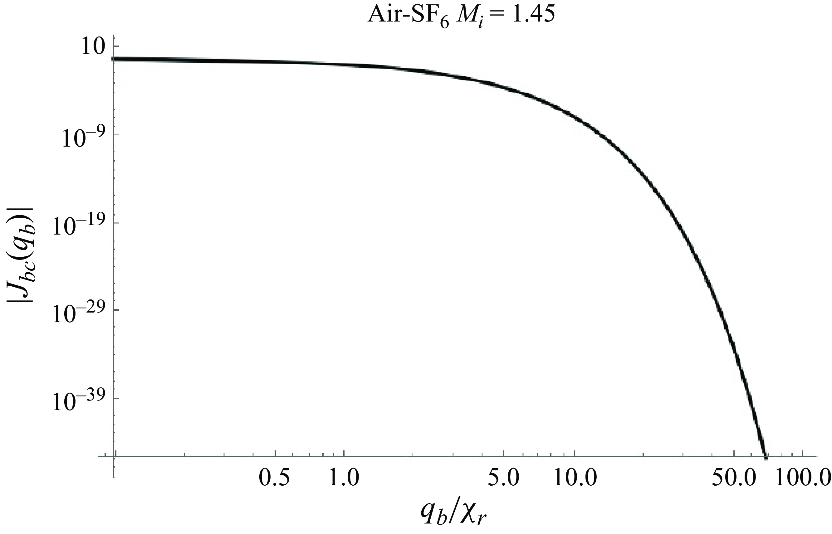
for simplicity. In figure 4 we show
 $|J_{c}(q_b)|$
for the gas and shock parameters indicated, evaluated with coefficients
 $\omega _{b \nu }$
inside (5.13), because the simplest way of evaluating
 $J_{c}$
is using the infinite series
 \begin{equation} J_c(q_b) = \sum _{\nu = 1}^{\infty } \omega _{b \nu } \ \ e^{-\nu q_b }. \end{equation}
Behaviour of
 $|J_{c}(q_b)|$
as a function of
 $q_b$
for the parameters indicated.

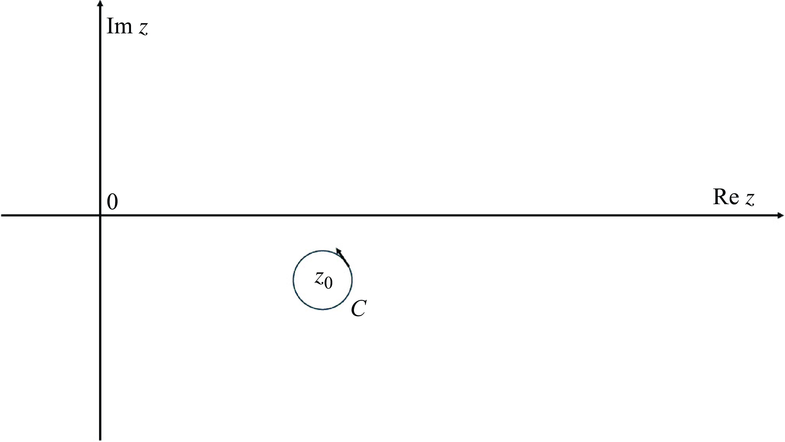
Contour of integration
 $C$
in the complex plane, used in (8.1).

Later on, we will derive an explicit analytic expression for
 $J_c(q_b)$
. It is convenient that we plot
 $J_c(q_b)$
. This is shown in figure 3. The plot in figure 3 was computed with 51 terms inside the sum. As for the corresponding function at the reflected shock, it is easy to see that
 \begin{equation} J_r(q_b) = \sum _{\nu = 1}^{\infty } E_{\nu }(\chi _r) e^{-\nu q_b} , \end{equation}
where the coefficients
 $E_{\nu }(\chi _r)$
have been defined in (4.15).
We see, from figure 3, that
 $J_{\textit{bc}}(q_b) \sim 0$
, for
 $q_b \geqslant \chi _r$
. Similarly inside fluid a:
 $J_{ac}(q_a ) \sim 0$
, because of normal velocity continuity at the rippled surface. This fact will allow us later on to get a simplified (albeit approximate) system of functional equations for
 $P_r(q_b)$
and
 $P_t(q_a)$
, much simpler than equations (65, 66) of Wouchuk (Reference Wouchuk2001a
). This means that we can approximate:
 $F_{b1}(q_b) \sim F_{b2}(q_b)$
, for
 $q_b\gt \chi _r$
and
 $F_{a1}(q_a) \sim F_{a2}(q_a)$
for
 $q_a\gt | \chi _t |$
. This behaviour allows us to approximate:
 $F_{m1}(q_m) \sim F_{m2}(q_m)$
. This approximation is called here the RPA, because, for a true rigid piston, as in Wouchuk (Reference Wouchuk2025), the equality between both functions holds exactly:
 $F_{m1}(q_m) = F_{m2}(q_m)$
. The RPA will become very useful later on to construct decoupled functional equations satisfied by the pressure perturbations at both shock fronts.
We proceed next by writing the linearised Rankine Hugoniot equations at each corrugated shock. We recall again that we work in a reference system that comoves with the velocity
 $U$
of the shocked contact surface.
6. Linearised Rankine Hugoniot equations
The time evolution of the reflected shock ripple amplitude,
 $\psi _r(\tau )$
, is governed by the pressure fluctuations behind the reflected shock, through the equations
 \begin{align} \frac {\partial \psi _r}{\partial \tau _b} &= A_{sr} \psi_0 \hat {p}_r , \end{align}
 \begin{align} A_{sr} &= \frac {R_{\textit{refl}}}{R_{\textit{refl}}-1} \frac {M_r^2-1}{2 M_r^2 \beta _r} . \end{align}
At any value of the dimensionless time
 $\tau _b$
, conservation of tangential momentum across the reflected shock (Landau & Lifshitz Reference Landau and Lifshitz1986) is responsible of generating the corresponding tangential velocity perturbation behind it
 \begin{equation} v_r(\tau _b) = \frac {U_1-U}{D_i} \psi _r . \end{equation}
The density perturbations are related to the pressure perturbations through the equations
 \begin{align}\begin{split} \hat {\rho }_r(r) &= A_{\rho r} \ \hat {p}_r(r) , \\ A_{\rho r} &= \frac {1}{2 M_r^2 \ \beta _r^2} . \end{split}\end{align}
It is understood that these functions are evaluated just behind the corrugated shock, that is, at
 $\chi = \chi _r$
.
The longitudinal velocity behind the reflected shock is given by
 \begin{align} \begin{split} u_r(r) &= A_{\textit{xr}} \ \hat {p}_r(r) , \\ A_{\textit{xr}} &= \frac {M_r^2+1}{2 M_r^2 \beta _r} . \end{split} \end{align}
Behind the transmitted front we have, similarly
 \begin{eqnarray} u_t(r) &=& A_{\textit{xt}} \ \hat {p}_t(r) , \nonumber \\ A_{\textit{xt}} &=& \frac {M_t^2+1}{2 M_t^2 \beta _t} . \end{eqnarray}
The dimensionless tangential velocity behind the reflected shock, in units of the incident shock speed, is
 \begin{equation} v_r(\tau ) = \frac {U_1- U}{D_i} \psi _r(\tau ) . \end{equation}
Similarly, the tangential velocity perturbation behind the transmitted front is
 \begin{equation} v_t(\tau ) = -\frac {U}{D_i} \psi _t(\tau ) . \end{equation}
The time evolution of the transmitted shock ripple amplitude,
 $\psi _t(\tau )$
satisfies the equations
 \begin{align}\begin{split} \frac {\partial \psi _t}{\partial \tau _a} &= A_{st} \psi _0 \hat {p}_t , \\ A_{\textit{st}} &= \frac {R_{\textit{tr}}}{R_{\textit{tr}}-1} \frac {M_t^2-1}{2 M_t^2 \beta _t} . \end{split} \end{align}
The density perturbations behind the transmitted shock are related to the pressure perturbations through the equations
 \begin{align} \begin{split} \hat {\rho }_t(r) &= A_{\rho t} \ \hat {p}_r(r) , \\ A_{\rho t} &= \frac {1}{2 M_t^2 \ \beta _t^2} . \end{split}\end{align}
To solve the linear perturbation problem we will solve for the Laplace transforms
 $P_r(q_b)$
and
 $P_t(q_a)$
.
The best strategy is to follow Richtmyer (Reference Richtmyer1960) and take the time derivative of (6.5) and of (6.6) following the reflected and transmitted shocks, respectively. For the reflected shock, we get the relationship (from now on, we use the notation:
 $\xi _r = k \psi _r$
,
 $\xi _t = k \psi _t$
)
 \begin{equation} j_r(r_b) = -A_{\textit{xr}} \frac {\partial \hat {p}_r}{\partial r} + A_{yr} \beta _r \xi _r , \end{equation}
where
 $A_{yr} = ({U_1- U})/{D_i}$
. The subscript
 $r$
indicates that the function
 $j$
is evaluated just behind the reflected front, at
 $\chi = \chi _r$
. If we take the Laplace transform of (6.11), we obtain
 \begin{equation} J_r(q_b) = \alpha _{b1}(q_b) \ P_r(q_b) + \alpha _{b2}(q_b) , \end{equation}
which is equivalent to (2.25) of Wouchuk (Reference Wouchuk2025), where
 \begin{equation} \alpha _{b1}(q_b) = \alpha _{b10} \sinh q_b + \frac {\alpha _{b11}}{\sinh q_b} , \end{equation}
with
 \begin{align} \alpha _{b10} &= - A_{\textit{xr}} , \end{align}
 \begin{align} \alpha _{b11} &= -\frac {1}{2 \beta _r} . \end{align}
Similarly for the transmitted shock
 \begin{equation} J_t(q_a) = \alpha _{a1}(q_a) \ P_t(q_a) + \alpha _{a2}(q_a) , \end{equation}
with
 \begin{eqnarray} \alpha _{a1}(q_a) &=& \alpha _{a10} \sinh q_a + \frac {\alpha _{a11}}{\sinh q_a} , \end{eqnarray}
where
 \begin{equation} \alpha _{a10} = -\frac {M_t^2+1}{2 M_t^2 \beta _t} , \end{equation}
and
 \begin{equation} \alpha _{a11} = -\frac {1}{2 \beta _t} . \end{equation}
It is convenient that we recall here the behaviour of the functions
 $J_{ac}(q_a)$
and
 $J_{\textit{bc}}(q_b)$
as functions of
 $q_a, q_b$
, respectively. To this end we must pay attention to figure 3. Please note that, because of normal velocity continuity at the contact surface, this relationship holds:
 $J_{\textit{bc}}(q_b) \equiv J_{\textit{bc}}(q_b) =J_{ac}(q_a) \equiv J_{ac}(q_a)$
, where
 $q_a$
and
 $q_b$
are related by
 $ Q \sinh q_a= \sinh q_b$
. For simplicity, we define
 $J_c(q_b) = J_{\textit{bc}}(q_b).$
In figure 3 we show the function
 $J_{\textit{c}}(q_b)$
for the pre-shock parameters indicated.
Motivated by figure 3, we make the approximations
 \begin{align} \begin{split} J_{ac}(q_a) &\sim 0, (q_a\geqslant 1) , \\ J_{\textit{bc}}(q_b) &\sim 0, (q_b \geqslant 1) . \end{split} \end{align}
For a truly rigid piston surface, the function
 $J_c$
is exactly equal to zero (Wouchuk Reference Wouchuk2001a
; Reference Wouchuk2025), therefore, if we make
 $J_c(q_m) \sim 0$
, for a real contact surface, this is only an approximation, which will be called a RPA. It is emphasised here that the RPA embodied in (6.20) constitutes an approximation that may fail if the gases and/or shock Mach are varied and this will have an influence when we calculate the terminal velocity, as it might be a source of error. The error incurred in the calculation of the terminal velocity because of assuming (6.20) will be analysed with detail in § 16 after the results for the terminal velocity are presented.
7. Functional equations satisfied by
 $\boldsymbol{P_r(q_b)}$
and
$\boldsymbol{P}_{\boldsymbol{t(q_a)}}$


Let us briefly recall the relationship between
 $J_r$
and
 $P_r$
 \begin{equation} J_r(q_b) = \alpha _{b1}(q_b) P_r(q_b) + \alpha _{b2}(q_b) .\end{equation}
If in (5.6) we use the above presented approximations (
 $F_{b1} \sim F_{b2}$
,
 $F_{a1} \sim F_{a2}$
), we easily arrive to the following functional equation for
 $P_r(q_b)$
:
 \begin{equation} P_r(q_b) = \lambda _{b1}(q_b) + \lambda _{b2}(q_b) P_r(q_b + 2 \chi _r) . \end{equation}
The auxiliary functions are
 \begin{align} \lambda _{b1}(q_b) &= \frac {\alpha _{b2}(q_b) + \alpha _{b2}(q_b+2 \chi _r)}{\cosh q_b - \alpha _{b1}(q_b)} , \end{align}
 \begin{align} \lambda _{b2}(q_b)&= \frac {\alpha _{b1}(q_b + 2 \chi _r) + \cosh (q_b + 2 \chi _r)}{\cosh q_b - \alpha _{b1}(q_b)} . \end{align}
We notice here that
 $\lambda _{b1,2}$
above are exactly the same functions shown in (44) and (45) of Wouchuk (Reference Wouchuk2001a
), and (36a, 36b) of Wouchuk (Reference Wouchuk2025) which is no surprise, because for a rigid piston, the relationships
 $F_{b1} = F_{b2}, F_{a1} = F_{a2}$
, hold exactly.
We proceed in the same manner with the transmitted shock and arrive at a similar functional equation for
 $P_t(q_a)$
 \begin{equation} P_t(q_a) = \lambda _{a1}(q_a) + \lambda _{a2}(q_a) P_t(q_a-2 \chi _t) , \end{equation}
where
 \begin{align} \lambda _{a1}(q_a) &= -\frac {\alpha _{a2}(q_a) + \alpha _{a2}(q_a - 2 \chi _t)}{\cosh q_a + \alpha _{a1}(q_a)} , \end{align}
 \begin{align} \lambda _{a2}(q_a) &= \frac {\cosh (q_a - 2 \chi _t) - \alpha _{a1}(q_a - 2 \chi _t)}{\cosh q_a + \alpha _{a1}(q_a)} . \end{align}
We notice here two important facts
 \begin{align}\begin{split} & \lambda _{a2}(q_a = 0) =0, \\ & \lambda _{b2}(q_b = 0) = 0 . \end{split}\end{align}
It is mentioned here that for ideal gas equation of state (EOS), the denominators of the auxiliary functions (
 $\lambda _{a1,2}, \lambda _{b1,2}$
) above never vanish, which means that
 $P_r$
and
 $P_t$
do not have poles and hence they are analytic functions of their arguments in the complex plane. Therefore, in such a case, the phenomenon of spontaneous acoustic emission (SAE) is excluded (Wouchuk & Cavada Reference Wouchuk and Cavada2004). However, SAE might occur for other EOS, as shown in Wouchuk & Cavada (Reference Wouchuk and Cavada2004), Calvo-Rivera, Velikovich & Huete (Reference Calvo-Rivera, Velikovich and Huete2023) and Napieralski et al. (Reference Napieralski, Cobos, Velikovich and Huete2024) The functional equations presented above are extremely difficult solve exactly and different methods have been tried in the past to extract useful information from them (Wouchuk Reference Wouchuk2001a
, Reference Wouchuk2025). In this work, and thanks to the analyticity of the functions
 $P_r$
and
 $P_t$
in the complex plane, we can show the exact solutions of (7.2) and (7.5). We show this solution in the following section.
8. Exact solution of the functional equations (7.2) and (7.5)
We need some concepts from calculus in one complex variable. We refer to the classical textbook of Churchill (Reference Churchill1974).
First, we recall the Cauchy integral formula (see page 129 of Churchill Reference Churchill1974). We consider a function
 $f$
that is analytic everywhere within and on a simple closed contour
 $C$
oriented counterclockwise. If
 $z_0$
is any point interior to
 $C$
, then, the Cauchy integral formula holds
 \begin{equation} f(z_0) = \frac {1}{2 \pi i} \int _{C} \frac {f(z)}{z-z_0} {\rm d}z , \end{equation}
where
 $i$
is the imaginary unit.
As discussed before, our functions of interest
 $P_r(q_b)$
, and
 $P_t(q_a)$
are analytic functions in their corresponding complex planes. Hence, (8.1) can be used with both of them. The idea is straightforward: we divide both members of (7.2) by
 $2 \pi i\ (q_b-q_0)$
where
 $q_0$
is an arbitrary complex number, and integrate along a curve
 $C$
centred at
 $q = q_0$
. We arrive at the equation
 \begin{equation} \frac {1}{2 \pi i} \int _{C} \frac {P_r(q_b)}{q_b-q_0} {\rm d}q = \frac {1}{2 \pi i} \int _{C} \frac {\lambda _{b1}(q_b)}{q_b-q_0} {\rm d}q_b + \frac {1}{2 \pi i} \int _{C} \frac {\lambda _{b2}(q_b) P_r(q_b + 2 \chi _r)}{q-q_0} {\rm d}q_b . \end{equation}
Thanks to the analyticity of
 $P_r$
, the contour of the last integral in the above equation can be deformed in such a way to make
 $q_0 = 0$
, and hence, the contour
 $C$
is centred at the origin (but only for the last integral inside (8.2)) Hence, (8.1) can be immediately applied, and recalling that
 $\lambda _{b2}(q_b = 0) = 0$
, we get
 \begin{equation} P_r(q_0) = \lambda _{b1}(q_0) . \end{equation}
As
 $q_0$
is an arbitrary complex number in the above equation, we deduce
 $P_r(q_b) = \lambda _{b1}(q_b)$
for any complex number
 $q_b$
. Similar arguments hold for the transmitted shock and we deduce
 \begin{equation} P_t(q_a) = \lambda _{a1}(q_a) . \end{equation}
It is very important to notice that the functions
 $\lambda _{m1,2}(q_m)$
are not independent of each other. They are related because of the Rankine Hugoniot equations, through the auxiliary coefficients
 $\alpha _{m10}, \alpha _{m11}$
. This means that the solution obtained for the above functional equations (7.2, 7.5), may not be generalised to arbitrarily created functional equations. Let us consider, for example, the following, totally invented equation, to illustrate with an example:
 \begin{equation} f(x) = \cos x + \sin x \ f(x+\pi /2) . \end{equation}
It is clear that
 $\cos x, \sin x$
are analytic in the whole complex plane, and
 $\sin 0 =0$
. However, this does not mean that the solution to the above equation is
 $f(x) = \cos x$
as can be easily verified. Anyway, the method described in § 8, might be of help for other functional equations, with proper modifications, depending on the particular functional equation to be solved. The key point in § 8 has been the analyticity of all the functions appearing in the functional equations. We can compare the solution obtained above for
 $P_r$
with the solution for
 $P_r(q_b)$
expressed as a series of decaying exponentials, obtained after solving the corresponding wave equation by separation of variables. This comparison is shown in figure 5(a,b) for the shock and fluid parameters indicated. Before proceeding to calculate the terminal velocity, it is necessary to pay attention to the following fact: the function
 $\lambda _{a1}(q_a)$
, if evaluated at
 $q_a = \chi _t$
, gives
 $\lambda _{a1}(\chi _t) = 0$
. As a consequence, the flux of the vorticity generated by the transmitted shock, represented by the quantity
 $F_a$
defined in (9.28), will be identically zero. This absurd result has a tragic consequence: it will lead to an intolerable error in the terminal velocity calculation. If
 $F_a = 0$
is plugged into (9.28), will give a very poor comparison with the linear simulations of Yang et al. (Reference Yang, Zhang and Sharp1994). This does not mean that (8.4) is incorrect. The solution found to the functional equations is correct. The problem of getting
 $F_a = 0$
is because the functional equations themselves are approximate. They have been obtained after approximating
 $J_{mc}(q_m) \sim 0$
on each side of the contact surface, that is, using the RPA. This problem did not arise in Wouchuk (Reference Wouchuk2001a
), because the complete boundary conditions at the contact surface had been used in that work. The only way to circumvent this serious nuisance here has been to iterate once on the trial function defined below. That is, in order to calculate the quantity
 $F_a$
to be plugged in (9.28), we use the iterated function
 \begin{equation} P_{t1}(q_a) = \lambda _{a1}(q_a) + \lambda _{a2}(q_a) P_{\textit{ttrial}}(q_a-2 \chi _t) . \end{equation}
The function
 $P_{\textit{ttrial}}(q_a)$
is built using the RPA. That is, motivated by (43, 44) of Wouchuk (Reference Wouchuk2025) we use
 \begin{equation} P_{\textit{ttrial}}(q_a) = D_{t1} \frac {e^{-q_a}}{\cosh q_a} , \end{equation}
where the coefficient
 $D_{t1}$
is taken from Wouchuk (Reference Wouchuk2025)
 \begin{equation} D_{t1} = \frac {2 \alpha _{a20}}{\beta _t - \alpha _{a10} \cosh \chi _t} . \end{equation}
(a) Comparison of the function
 $P_{r1}(q_b)$
defined in (8.11) with the corresponding Bessel series (5.11), for the gases and Mach number indicated. The quantity
 $P_{r0} = \lim _{q_b \rightarrow 0} [\lambda _{b1}(q_b)]$
(b) A similar comparison, but for the function
 $J_r(q_b)$
, defined in (6.12) and in (7.1),
 $J_{r0} = \lim _{q_b \rightarrow 0} [J_r(q_b)]$
.

Later on, we will see that, in order to calculate the temporal evolution of the shock pressure perturbations at the reflected shock, and compare with the Bessel series solution given by (4.12), we will also need to iterate once on a adequately chosen trial function at the reflected shock, in the same way as has been done above for the transmitted shock. We define similarly for the reflected shock
 \begin{equation} P_{\textit{rtrial}}(q_b) = D_{r1} \frac {e^{-q_b}}{\cosh q_b} , \end{equation}
where, analogously to
 $D_{t1}$
, we have
 \begin{equation} D_{r1} = \frac {2 \alpha _{b20}}{\beta _r- \alpha _{b10} \cosh \chi _r}. \end{equation}
Therefore, to calculate the temporal evolution of the reflected shock pressure perturbations, we use the function
 \begin{equation} P_{r1}(q_b) = \lambda _{b1}(q_b) + \lambda _{b2}(q_b)P_{\textit{rtrial}}(q_b+ 2 \chi _r) . \end{equation}
With the function
 $P_{r1}(q_b)$
above, we define
 $J_{r1}(q_b)$
 \begin{equation} J_{r1}(q_b) = \alpha _{b1}(q_b) P_{r1}(q_b) + \alpha _{b2}(q_b) . \end{equation}
The functions
 $P_{r1}(q_b)$
and
 $J_{r1}(q_b)$
are compared with the corresponding Bessel series in figure 5.
Referring to figure 5, we see that the iterated solution
 $P_{r1}(q_b)$
, as given above agrees very well with the solution given by (5.11), and the function
 $J_{r1}(q_b)$
also agrees neatly with (7.1). For later purposes, when we study the growth of the contact surface ripple, it is necessary to show here the explicit form of the function
 $J_c(q_b)$
in terms of the solution found above for
 $P_r(q_b)$
. We recall that
 $J_c(q_b) = F_{b1}(q_b) - F_{b2}(q_b)$
. Hence, from (5.6), we get
 \begin{align} J_c(q_b) &= J_{r1}(q_b+\chi _r) + J_{r1}(q_b-\chi _r) +\cosh (q_b+ \chi _r) P_{r1}(q_b+\chi _r) \nonumber \\ &\quad - \cosh (q_b-\chi _r) P_{r1}(q_b-\chi _r) . \end{align}
The above expression for
 $J_c(q_b)$
will be necessary later on to analyse the asymptotic contact surface ripple growth in § 15, and also to estimate the relative error in the calculation of the terminal velocity in § 16.
9. Inverse Laplace transforms
In order to compute
 $\hat {p}_r(r)$
and
 $\hat {p}_t(r)$
in the domains of the corresponding variable
 $r$
, we must invert the functions
 $P_r(q_b)$
and
 $P_t(q_a)$
by contour integration in the complex plane. We start with the reflected shock (Zwillinger Reference Zwillinger1983; Wouchuk Reference Wouchuk2025).
The integral that corresponds to
 $\hat {p}_r(r)$
is given by
 \begin{equation} \hat {p}_r(r_b) = \frac {1}{2 \pi i}\int _{\mathcal{C}} P_r(s_b) e^{s_b r_b} , \end{equation}
where the contour of integration C is located to the right of the singularities of
 $P_r$
, that is, in the semiplane
 $Re{s}\gt 0$
, and
 $i$
is the imaginary unit:
 $i^2 = -1$
, as indicated in figure 5. As the procedure to calculate the above integral has been thoroughly detailed recently in Wouchuk (Reference Wouchuk2025), it will not be repeated here. Anyway, those details can also be found on any textbook on the subject like that of Sneddon (Reference Sneddon1972).
It is worth recalling here that the only singularities exhibited by
 $P_r, P_t$
are not poles, but branch points at
 $s_m = \pm i$
. The origin of the branch points is the square root term
 $\sqrt {s^2+1}$
originating from
 $\cosh q$
, which in turn originates from the term
 $r \ \hat {p}_m(r)$
on the left-hand side of (4.10) that comes from the conservation of tangential momentum. As discussed in Huete et al. (Reference Huete, Wouchuk, Canaud and Velikovich2012), these branch points are responsible for the late time decay
 $p_r(r) \sim r^{-3/2}$
at large times, a behaviour already noticed by Fraley in Fraley (Reference Fraley1986). As an important conclusion, we can say that the asymptotic late time decay as
 $r^{-3/2}$
is caused by the lateral sound waves travelling parallel to shock surfaces (Fraley Reference Fraley1986).
Before calculating the integral of (9.1), we adopt the following conventions:
 $P_r^{+}(s)$
corresponds to the value of
 $P_r$
that results when considering the positive determination of the square roots of the form
 $\sqrt {s_b^2+1}$
inside
 $\lambda _{b1}(q_b)$
and
 $\lambda _{b2}(q_b)$
. Analogously,
 $P_r^{-}(s)$
is obtained considering the negative determination
 $-\sqrt {s^2+1}$
of the term
 $\cosh q_b$
After some algebra, we arrive at
 \begin{align} \hat {p}_r(r) &= \int _{-1}^{+1} f_{\textit{rc}}(z_b) \cos ( (z_b r) \ {\rm d}z_b , \end{align}
 \begin{align} &\quad + \int _{-1}^{+1} f_{\textit{rs}}(z_b) \sin (z_b r) \ {\rm d}z_b , \end{align}
with
 \begin{align} f_{\textit{rc}}(z_b) &= -\frac {1}{2 \pi } \textrm{Re}\left [D_r(z_b)\right ]\! , \end{align}
 \begin{align} f_{\textit{rs}}(z_b) &= \frac {1}{2 \pi } \textrm{Im}\left [D_r(z_b)\right ]\! , \end{align}
and
 $D_r(z_b) = P_r^{-}(i z_b) - P_r^{+}(i\ z_b)$
. Before proceeding, it is important to mention here the initial condition
 $\hat {p}_r(r = 0) = 0$
, as discussed by Richtmyer in Richtmyer (Reference Richtmyer1960). It can be seen that
 $f_{\textit{rc}}(z) = 0$
in (9.5) for any choice of the pre-shock parameters, which, when plugged into (9.3) ensures
 $\hat {p}_r(r = 0) = 0$
.
In figure 7, we show
 $p_r(r)$
, calculated with (9.3). Similar calculations allow us to write an analogous compact form of
 $\hat {p}_t(r)$
 \begin{align} \hat {p}_t(r) &= \int _{-1}^{+1} f_{\textit{tc}}(z_a) \cos (z_a r) {\rm d} z_a , \end{align}
 \begin{align} &\quad + \int _{-1}^{+1} f_{\textit{ts}}(z_a) \sin (z_a r) \ dz_a , \end{align}
Bromwich contour used to invert the Laplace transforms
 $P_r, P_t$
.


with
 \begin{align} f_{\textit{tc}}(z_a) &= -\frac {1}{2 \pi } \textrm{Re}\left [D_t(z_a)\right ]\! , \\[-12pt] \nonumber \end{align}
 \begin{align} f_{\textit{ts}}(z_a) &= \frac {1}{2 \pi } \textrm{Im}\left [D_t(z_a)\right ] \!, \\[9pt] \nonumber \end{align}
and
 $D_t(z_a) = P_t^{-}(i \ z_a) - P_t^{+}(i\ z_a)$
. Similarly to the reflected shock, it can be seen that
 $f_{\textit{tc}}(z) = 0$
.
Referring to figure 7, we mention that it is almost impossible to calculate
 $p_r(r_b), p_t(r_a)$
for very large times with the series of Bessel functions, because of the accumulation of round-off errors. It is important to notice that the inverse Laplace transformation procedure has been performed on the iterated function
 $P_{r1}(q_b)$
. Inverting only
 $\lambda _{b1}(q_b)$
gives a poor comparison with the Bessel series solution. The reason is easy to understand: in any RMI problem, there is a strong interaction between the shock fronts and the contact surface, via sonic reverberations. These sonic reverberations are mathematically taken into account in the functional equation for the Laplace transforms inside the shifted arguments of
 $P_r(q_b+ 2 \chi _r)$
, and
 $P_t(q_a-2 \chi _t)$
. As discussed in Wouchuk & Cavada (Reference Wouchuk and Cavada2004), the origin of the shifts
 $2 \chi _r, 2 \chi _t$
is due to the Doppler shift, i.e. to the sonic reverberations. This is why agreement improves when using the iterated function
 $P_{r1}(q_b)$
as written in (8.11). Having established the way to invert the Laplace transforms we can proceed now to calculate the asymptotic velocity profiles inside each fluid. To this end we need the vorticity generated by each rippled front. To calculate the vorticity, we recall the important fact that tangential momentum across each rippled front is conserved, and this mechanism is responsible of generating a tangential velocity perturbation behind the corrugated shock, see (6.7, 6.8), which in turn is the way vorticity is created; see Wouchuk (Reference Wouchuk2001a
), Cobos-Campos & Wouchuk (Reference Cobos-Campos and Wouchuk2016) and Wouchuk (Reference Wouchuk2025). The important consequence is that the velocity fields generated by the corrugated fronts are of rotational nature. We recall here the definition of the
 $z$
- component of vorticity
 \begin{equation} \delta \omega (x,y) = \frac {\partial \delta v_y}{\partial x} - \frac {\partial \delta v_x}{\partial y} . \end{equation}
We must pay attention to the fact that vorticity is only generated at each corrugated shock. Once it is created, in the absence of viscosity, the vorticity attached to the fluid element does not change in time. That is, the time derivative of
 $\delta \omega$
following the fluid element is zero:
 ${\rm d}\delta \omega /{\rm d} \tau = 0$
, which, in linear theory, reads
 $\partial \ \delta \omega / \partial \tau = 0$
. That is, the vorticity field is steady state and hence only a function of space coordinates
 $(x, y)$
. Let us start with the reflected shock: we define the dimensionless characteristic time
 $\tau _0(x) = kx/\beta _r$
as the time needed by the reflected shock to arrive at position
 $x$
. Associated with
 $\tau _0$
, the value of the corresponding variable
 $r$
is
 \begin{equation} r_0(x) = \frac {k x}{\sinh \chi _r} = \frac {kx }{\beta _r} \sqrt {1-\beta _r^2} . \end{equation}
Therefore, in order to compute the vorticity at position
 $(x, y)$
we must get the values of the partial derivatives
 $\partial \delta v_y/\partial x$
and
 $\partial \delta v_x/\partial y$
at the time
 $\tau _0$
behind the reflected shock. To this end we use the conservation of tangential momentum across the front, and differentiate with respect to time, following the reflected shock, that is, applying the differential operator
 ${\rm d}/{\rm d} \tau = \partial /\partial \tau + \beta _r \partial /\partial x$
at both sides of the equation that defines
 $v_r$
 \begin{equation} v_r(\tau ) = \frac {U_1-U}{D_i} \psi _r(\tau ) . \end{equation}
After some algebra, the value of
 $ (\partial v/ \partial x )_{x_r}$
is readily obtained. The value of
 $\partial v_x/ \partial y$
is easily computed from (6.5). Collecting both results, we get
 \begin{equation} \omega _b(x, y) = g_b(x) \sin k y . \end{equation}
The function
 $g_b(x)$
is
 \begin{equation} g_b(x) = \varOmega _b \hat {p}_r \left (r_b = \frac {kx}{\sinh \chi _r} \right ) , \end{equation}
in which the constant
 $\varOmega _b$
is given by
 \begin{equation} \varOmega _b = \frac {(M_r^2-1)^2 }{M_r^2} \frac {\sqrt {\gamma _b M_r^2 - \gamma _b + 1}}{\left [(\gamma _b -1) M_r^2 + 2 \right ]^{3/2}} . \end{equation}
It is easy to see that, for a weak incident shock, the vorticity quantity
 $\Omega$
scales like:
 $\varOmega _b \sim z_i^2$
. Proceeding similarly with the transmitted shock, we write the vorticity stored inside fluid
 $a$
 \begin{equation} \omega _a(x, y) = g_a(x) \sin k y . \end{equation}
The function
 $g_a(x)$
is
 \begin{equation} g_a(x) = \varOmega _a \hat {p}_t \left (r_a = \frac {kx}{\sinh \chi _t}\right ) , \end{equation}
in which the constant
 $\varOmega _a$
is given by
 \begin{equation} \varOmega _a = \frac {(M_t^2-1)^2 }{M_t^2} \frac {\sqrt {\gamma _a M_t^2 - \gamma _a + 1}}{\left [(\gamma _a -1) M_t^2 + 2 \right ]^{3/2}} . \end{equation}
Please note that, inside fluid
 $a$
, the longitudinal cordinate
 $x$
is negative, i.e.:
 $x \lt 0$
, and therefore
 $\chi _t \lt 0$
. Hence, the argument
 $r_a$
inside
 $\hat {p_t}$
of (9.17) is positive. There is an important physical meaning of (9.14–9.17) above: the value of the vorticity generated at position
 $x$
is proportional to the shock pressure perturbations at the time
 $\tau _0(x)$
. In this sense, the vorticity stored in each compressed fluid is a memory of the compressible evolution of the corresponding shock front perturbations since
 $t = 0+$
. What is even more important is that the velocity field in the limit
 $t \rightarrow \infty$
must be consistent with this vorticity field, and hence, it will never be an irrotational field. The irrotationality assumption of the velocity fields will be approximate for an incident shock of negligible intensity.
As each of the shocks separate from the contact surface, their ripples oscillate in time with decaying amplitude. Meanwhile, the shocks fill the space between them with an acoustic field of pressure perturbations in both fluids,
 $\hat {p}_b(r_b, \chi _b), \ \hat {p}_a(r_a, \chi _a)$
, which also decrease to zero in the asymptotic limit
 $t \rightarrow \infty$
. Therefore, when the shocks are very far away, the fluid particles do not experience acceleration any more and the velocity field becomes steady state (Wouchuk & Nishihara Reference Wouchuk and Nishihara1996, Reference Wouchuk and Nishihara1997; Wouchuk Reference Wouchuk2001a
). Our immediate purpose now is to derive the differential equations that describe the asymptotic velocity fields in both fluids as functions of the spatial coordinates
 $x$
and
 $y$
: as has been shown for the first time in Wouchuk (Reference Wouchuk2001a
), the longitudinal velocity perturbations inside fluid
 $b$
satisfy the differential equation written immediately below (this equation is obtained by combining the linearised Euler equations) (Wouchuk Reference Wouchuk2001a
, Reference Wouchuk2025)
 \begin{equation} u_b^{\prime\prime}(x) - u_b(x) = -g_b(x) . \end{equation}
While the tangential velocity perturbations obey the equation
 \begin{equation} v_b^{\prime\prime}(x) - v_b(x) =g^{\prime}_b(x) . \end{equation}
Inside fluid
 $a$
, we have identical equations for
 $u_a(x)$
, and
 $v_a(x)$
 \begin{align} u_a^{\prime\prime}(x) - u_a(x) &= -g_a(x) , \end{align}
 \begin{align} v_a^{\prime\prime}(x) - v_b(x) &=g^{\prime}_a(x) . \end{align}
It is convenient to solve (9.19, 9.21) here to get the spatial profile of the velocity field.
As for the longitudinal velocity
 $u_b(x)$
inside the light fluid, the solution of (9.19) can be written as the solution of the homogeneous equation plus a particular solution. We propose then
 \begin{equation} u_b(x) = A e^{-x} + u_{\textit{bpart}}(x) . \end{equation}
As for the particular solution we propose
 \begin{equation} u_{\textit{bpart}}(x) = \int _{-1}^{+1} h_{bs}(z) \sin \frac {z x}{\sinh \chi _r} {\rm d}z . \end{equation}
Constant
 $A$
in (9.23) will be determined soon. As for the function
 $h_{bs}(z)$
entering in
 $u_{\textit{bpart}}$
, it can be calculated by plugging (9.24) into the left-hand side of (9.19). We also use (9.14). After simple inspection, we get
 \begin{equation} h_{bs}(z) = \frac {\varOmega _b \sinh ^2 \chi _r}{z^2+ \sinh ^2 \chi _r} f_{\textit{rs}}(z) .\end{equation}
Thanks to the fact that
 $\hat {p}_r(r =0+) =0$
, there is only a sine contribution in the integral decomposition for
 $\hat {p}_r$
, (9.3), which in turn gives only a sine contribution for the integral that defines
 $u_{\textit{bpart}}(x)$
in (9.24). Hence, the vanishing of the pressure perturbations behind the reflected shock at
 $t = 0+$
implies
 $u_{\textit{bpart}}(x = 0) = 0$
. Therefore, the constant
 $A$
in (9.23) is
 $A = u_c^{\infty }$
.
The tangential velocity perturbations are obtained by differentiating (9.23):
 $v_b(x) = -u_b'(x)$
.
The fact that the pressure perturbations vanish asymptotically in time has a profound consequence: given that
 $\partial \delta \rho / \partial \tau = \partial \delta p/ \partial \tau$
, because of entropy conservation (Landau & Lifshitz Reference Landau and Lifshitz1986), we deduce that, when the shocks are infinitely apart from the contact surface, the velocity fields of both fluids become incompressible, independently of the values of
 $\gamma _a, \gamma _b$
and
 $M_i$
. This means that
 $v(x) = -u'(x)$
in both fluids. The differential equations above can then be integrated inside the interval
 $0 \lt x \lt \infty$
using the Laplace transforms of the functions
 $P_r$
and
 $P_t$
, as will be shown soon. Let us multiply both members of (9.21) by
 $e^{-\sigma x}$
, with
 $\sigma$
a positive real number yet to be determined . After integration by parts and using the asymptotic incompressibility commented on above, we define, for fluid
 $b$
, the function
 $U_b(\sigma )$
: (Wouchuk Reference Wouchuk2001a
, Reference Wouchuk2025)
 \begin{equation} U_b(\sigma )= \int _0^{\infty } u(x) e^{-\sigma x} {\rm d}x = \frac {\sigma u_c^{\infty } - v_{\textit{bc}}^{\infty } - \varOmega _b \ \sinh \chi _r \ P_{r}(s_b = \sigma \sinh \chi _r)}{\sigma ^2-1} , \end{equation}
where
 $u_c^{\infty }$
is the asymptotic dimensionless longitudinal velocity at the contact surface ripple, and
 $v_{\textit{bc}}^{\infty }$
is the dimensionless tangential velocity, also at the position of the unperturbed contact surface (
 $x = 0$
) inside fluid b.
For ideal gases we do not have poles for
 $P_r$
and thus we do not expect poles for
 $U_b$
either. This is only possible if the numerator of (9.26) vanishes for
 $\sigma = 1$
. After rearranging terms, this condition leads us to the relationship
 \begin{equation} u_c^{\infty }-v_{\textit{bc}}^{\infty } = \varOmega _b \ \sinh \chi _r \ P_r \left (q_b = \chi _r \right ) \equiv F_b , \end{equation}
where
 $v_{\textit{bc}}^{\infty }$
is the asymptotic tangential velocity at the contact surface inside fluid b. It is only approximately equal to
 $u_c^{\infty }$
for a very weak shock, because
 $F_b \sim 0$
in that limit. The above condition relates the values of
 $u_c^{\infty }$
and
 $v_{\textit{bc}}^{\infty }$
to a particular integral of the shock pressure perturbations since
 $t = 0+$
up to
 $t = \infty$
. An important conclusion is that
 $u_c^{\infty }, v_{\textit{bc}}^{\infty }$
are never exactly equal.
Inside fluid
 $a$
, we multiply both members of (9.21) by
 $e^{\sigma } x$
and integrate inside the interval
 $-\infty \lt x \lt 0$
. Integrating by parts and proceeding as we did with
 $U_b(\sigma )$
, we arrive at an equation that relates the longitudinal and tangential velocities at the contact surface, but on side
 $a$
 \begin{equation} F_a = v_{ac}^{\infty }+ u_c^{\infty } = \varOmega _a \sinh \chi _t P_t(q_a = \chi _t) \equiv F_a, \end{equation}
where
 $v_{ac}^{\infty }$
is the asymptotic tangential velocity at the contact surface, inside fluid a. Once we compute the values of
 $F_a, F_b$
, we get the value of
 $u_c^{\infty }$
, the purpose of this work.
The procedure to obtain
 $u_c^{\infty }$
from the values of
 $F_a, F_b$
has been already explained in Wouchuk & Nishihara (Reference Wouchuk and Nishihara1997) but it is briefly recalled here. Thanks to the continuity of pressure at the contact surface, we equate the
 $y$
components of the Euler equations, on both sides of the contact surface, and write
 \begin{equation} \rho _{\textit{af}} \frac {\partial v_{a}(\tau )}{\partial \tau } = \rho _{\textit{bf}} \frac {\partial v_b(\tau )}{\partial \tau } . \end{equation}
If we integrate from
 $\tau = 0$
, up to
 $\tau = \infty$
, we get
 \begin{equation} R (v_{ac}^{\infty } - v_{a0}) = v_{\textit{bc}}^{\infty }- v_{b0} , \end{equation}
where
 $v_{b0}, v_{a0}$
are the initial tangential velocities behind the reflected and transmitted shocks, respectively. Combining (9.27–9.30), we solve for the normal velocity
 \begin{equation} u_c^{\infty } = \frac {v_{b0} - R v_{a0}}{R+1} + \frac {R F_a - F_b}{R+1} . \end{equation}
We see that that the asymptotic normal velocity is composed of the two terms indicated above. If there were no vorticity stored inside each fluid, the quantities
 $F_a, F_b$
would vanish, and hence only the term containing
 $v_{a0}, v_{b0}$
would be enough to compute
 $u_c^{\infty }$
. This is why we like to call it
 $u_{\textit{irrot}}$
, as it would be the only contribution for a perfectly irrotational velocity field
 \begin{equation} u_{\textit{irrot}} = \frac {v_{b0} - R v_{a0}}{R+1} . \end{equation}
Of course, this will never happen, because the term containing
 $F_a, F_b$
is important in the general case, especially at high compressions. Here, we see the need to calculate the Laplace transforms
 $P_r, P_t$
.
By the same token, we define
 \begin{equation} u_{\textit{rot}} = \frac {R F_a - F_b}{R+1} , \end{equation}
and we formally write
 \begin{equation} u_c^{\infty } = u_{\textit{irrot}} + u_{\textit{rot}} . \end{equation}
To compute
 $u_{\textit{rot}}$
, we need
 $F_a, F_b$
. Here,
 $F_a$
is calculated using the iterated function
 $P_{t1}$
, given in (8.6), and
 $F_b$
is evaluated using
 $P_{r1}$
as written in (8.11). In Wouchuk (Reference Wouchuk2001a
) a highly accurate iterative procedure to compute
 $F_a, F_b$
was developed, by solving exactly the boundary conditions at both shocks and at the contact surface. However, that iteration scheme is of a rather complicated algebraic structure. It is complicated system of coupled functional equations for
 $F_{a1}(q_a), F_{a2}(q_a)$
, and
 $F_{b1}(q_b), F_{b2}(q_b)$
, but the procedure to solve those equations in Wouchuk (Reference Wouchuk2001a
) did not involve any approximation like the RPA used here. Take a look, for instance, at equations (65) and (66) of Wouchuk (Reference Wouchuk2001a
).
The physical meaning of the quantities
 $F_a, F_b$
is simple: they represent the fluxes of the vorticity fields stored inside each fluid.
10. Comparison with the numerical work of Yang et al. (Reference Yang, Zhang and Sharp1994)
It is customary to compare, as we did in the past, with Yang et al. (Reference Yang, Zhang and Sharp1994). In this section we start comparing with the linear simulations of Yang et al. (Reference Yang, Zhang and Sharp1994). Before comparing we set some notation.
As shown in previous work (Wouchuk & Nishihara Reference Wouchuk and Nishihara1996), the normal velocity at the contact surface can be written, as a function of time, as
 \begin{equation} u_c(\tau _b) = u_c^{\infty } \int _0^{\tau _b} J_0(t) {{\rm d}t} + \sum _{n \geqslant 0} \omega _{b 2n+1} \left ( J_{2n+1}(\tau _b) + 2\sum _{k \geqslant 0}^{n-1}J_{2k+1}(\tau _b) \right ) , \end{equation}
where the coefficients
 $\omega _{b \nu }$
have been defined before; take a look, for instance, immediately after (4.13). The function
 $J_{\nu }(t)$
is the ordinary Bessel function of order
 $\nu$
. In figure 8 we compare our calculation of the ripple’s normal velocity as a function of time, (10.1) with the linear simulations of Yang et al. (Reference Yang, Zhang and Sharp1994).
The black continuous curve is calculated with (10.1). Red circles are from figure 7 of Yang et al. (Reference Yang, Zhang and Sharp1994), for the gases and shock Mach number indicated. The horizontal dashed black line is the terminal velocity
 $u_c^{\infty }$
calculated with (9.34).

In figure 8 we compare (10.1) with figure 7 of Yang et al. (Reference Yang, Zhang and Sharp1994). Our solution has been constructed including up to
 $\omega ^b_{51}$
inside the corresponding sums of (10.1). Besides this, we also compare below with table I of Yang et al. (Reference Yang, Zhang and Sharp1994). Table 1 is constructed in this way: for each pair of values (
 $R_0, s$
), the upper number in a row corresponds to the result of (9.31), while the lower one is the value shown in table I of Yang et al. (Reference Yang, Zhang and Sharp1994).
Ripple terminal velocities as given by (9.31) and the numerical simulations by Yang et al. (Reference Yang, Zhang and Sharp1994). The upper number in each entry is the result of this work and the lower one is the result shown in Table 1 of Yang et al. (Reference Yang, Zhang and Sharp1994). The adiabatic exponents are: (a)
 $\gamma _a = \gamma _b = 1.1$
, (b)
 $\gamma _a = \gamma _b = 3.0$
, (c)
 $\gamma _a = 3.0, \gamma _b = 1.5.$

From table 1 we see that our predictions are consistent with those of Yang et al. (Reference Yang, Zhang and Sharp1994), except for a few cases when the shock is very strong and/or
 $\gamma $
values are very different. The worst case scenario seems to be when
 $\gamma _a = 3.0$
,
 $\gamma _b = 1.5$
, for a very strong shock (
 $s \sim 1.0$
), with
 $R_{0}= 1.1$
for which the result of Yang et al. (Reference Yang, Zhang and Sharp1994) seems to indicate the proximity of freeze-out (Mikaelian Reference Mikaelian1991). We recall here again that the functionals (7.2, 7.5) are actually approximate equations, obtained with the RPA supported by figure 3, which motivated us to make
 $F_{b1}(q_b) \sim F_{b2}(q_b)$
, and hence to approximate
 $J_{cb}(q_b) \sim 0$
. Hence, even though we have obtained the exact solution of (7.2, 7.5), the equations themselves are only an approximation to the true equations satisfied by
 $P_r$
and
 $P_t$
. The RPA might break down when the Mach number increases without bound, or when the
 $\gamma$
values are very different on each side of the contact surface. We will later estimate the relative error ( which will be called
 $\eta _c$
) incurred in the calculation of
 $u_c^{\infty }$
, because of the assumption
 $J_c(q_b) \sim 0$
. We will study the dependence of
 $\eta _c$
as a function of
 $s$
and as a function of the
 $\gamma $
values. So far, the iteration procedure used in Wouchuk (Reference Wouchuk2001a
) gives more accurate estimates of
 $u_c^{\infty }$
than our estimate here. The reason seems to be clear: in Wouchuk (Reference Wouchuk2001a
), the system of functional equations embodied in (6.5 and 6.6) of that work are exact, as they involve the complete/exact boundary conditions at the shocks and the contact surface. This fact explains the good agreement observed between Wouchuk (Reference Wouchuk2001a
) and Yang et al. (Reference Yang, Zhang and Sharp1994). The solution presented here for
 $P_r$
and
 $P_t$
is appealing because of its simplicity, but is unfortunately tainted with an approximation that might break down for very strong shocks and/or very different gamma values.
To be clearer, our solution for
 $P_t(q_a) = \lambda _{a1}(q_a)$
, even though it is the exact solution of (7.5), predicts
 $P_t(\chi _t) = 0$
and hence,
 $F_a = 0$
, which is unphysical. This result is incorrect taking into account that
 $F_a$
becomes important for strong shocks and very different
 $\gamma $
values. In fact, following the iteration procedure explained in Wouchuk (Reference Wouchuk2001a
), for
 $\gamma _a = 3.0,\ \gamma _b = 1.5$
,
 $s \sim 1.0$
, we get, after some iterations:
 $F_a \sim 0.072 \neq 0, u_c^{\infty } \sim -0.0383$
in better agreement with Yang et al. (Reference Yang, Zhang and Sharp1994). The problem is actually with the approximation that supports (7.5) itself. Nevertheless, as will be seen later, reasonable agreement with experiments is obtained when analysing the ripple’s growth, within the time domain of validity for a linear theory, for relatively weak shocks.
It is important that we also compare with figure 11 of Yang et al. (Reference Yang, Zhang and Sharp1994).
In order not to overcrowd the figure, each case is shown as a separate plot in both figure 9 and figure 10. The values of
 $\gamma $
and
 $R_0$
are taken from Yang et al. (Reference Yang, Zhang and Sharp1994). The blue line is the prediction of
 $u_c^{\infty }$
here. Red circles are the simulation results of Yang et al. (Reference Yang, Zhang and Sharp1994). The black, dashed line is Fraley’s prediction given by (13.2), presented in Fraley (Reference Fraley1986); see the explanation near (13.2) for details. The blue line is always given by (9.31)
Terminal velocity as a function of shock strength
 $s$
for the gases indicated. Blue line is given by (9.31). Black dashed line is Fraley’s formula, (13.2), and red, empty circles are from figure 11 of Yang et al. (Reference Yang, Zhang and Sharp1994).

Terminal velocity as a function of shock strength
 $s$
for the gases indicated. Blue line is given by (9.31). Black dashed line is Fraley’s formula, (13.2), and red, empty circles are from figure 11 of Yang et al. (Reference Yang, Zhang and Sharp1994).

In all the cases shown in figure 9, and figure 10 the terminal velocity has been calculated with the RPA, and shown as the continuous blue line, as given by (9.31). The broken, black line is given by the formula presented by Fraley (Reference Fraley1986), according to the expressions derived by K. Mikaelian in Mikaelian (Reference Mikaelian1991), which is shown in this work as (13.2). Red empty circles are from Yang et al. (Reference Yang, Zhang and Sharp1994).
Red circles in figures 9–10 have been measured from figure 11 of Yang et al. (Reference Yang, Zhang and Sharp1994). In general, we see a reasonable agreement between our prediction and the numerical results of Yang et al. (Reference Yang, Zhang and Sharp1994), despite the unphysical prediction
 $F_a = 0$
. It is also important to note is that our prediction sensibly agrees with Fraley’s formula, as will be shown later on.
11. Weak shock limit
It is important to discuss the behaviour of the asymptotic velocity for very weak incident shocks.
To understand the behaviour of the terminal velocity in the limit
 $z_i\rightarrow 0$
, it is convenient to analyse the behaviour of the bulk vorticity quantities
 $F_a, F_b$
. To this end, it is very convenient to recall the representations as infinite series of decaying exponentials for
 $P_r, P_t$
, with the aid of (5.11)
 \begin{align} P_r(q_b) &:= \sum _{n = 0}^{\infty } D_{b 2n+1} \frac {e^{-(2n+1) q_b}}{ \cosh q_b} , \end{align}
 \begin{align} P_t(q_a) &:= \sum _{n = 0}^{\infty } D_{a 2n+1} \frac {e^{-(2n+1) q_a}}{ \cosh q_a}. \\[9pt] \nonumber \end{align}
We recall the formulas for
 $F_a, F_b$
, given in (9.28, 9.27)
 \begin{align}\begin{split} F_a &= - \varOmega _a \sinh \chi _t \ P_t(\chi _t) , \\ F_b &= \varOmega _b \sinh \chi _r \ P_r(\chi _r). \end{split} \end{align}
With the aid of Supplementary materials, it can be seen that
 $|D_{b \nu }| \lt |D_{b1}|$
. Hence, we can write
 \begin{equation} |F_b| \lt \varOmega _b \sinh \chi _r |D_{b1}| S_g(\chi _r)/ \cosh \chi _r , \end{equation}
where the function
 $S_g(q_b)$
is the sum of a geometric series
 \begin{equation} S_g(q_b) = \sum _{n = 0}^{\infty } e^{-(2 n + 1) q_b} = \frac {e^{ +q}}{e^{2 q} -1}. \end{equation}
Plugging in the above results into (11.3), we get, for the reflected shock
 \begin{equation} |F_b| \lt \varOmega _b \sinh \chi _r |D_{b1} |S_g(\chi _r)/ \cosh \chi _r . \end{equation}
In order to take the weak shock limit of the right-hand side of the above inequality, we recall the scaling of (2.30):
 $e^{- \chi _r} \sim \sqrt {z_i}$
, if
 $z_i \ll 1$
. Besides, coefficient
 $D_{b1}$
is linear in
 $z_i$
:
 $D_{b1} \sim z_i$
. From (9.15), we see that
 $\varOmega _a, \ \varOmega _b \sim z_i^2$
for very weak shocks. Plugging in all these scalings into the right-hand side of (11.6), we deduce:
 $F_b \sim z_i^{7/2}$
. And analogously for
 $F_a$
. On the other hand, it is not difficult to see that
 $u_{\textit{irrot}} \sim z_i$
. Therefore, for very weak shocks, the contribution of the bulk vorticity quantities
 $F_a, F_b$
can be safely neglected in comparison with
 $u_{\textit{irrot}}$
. Therefore, when considering the weak shock limit of
 $u_c^{\infty }$
, it is enough to expand
 $u_{\textit{irrot}}$
up to third order and neglect the vorticity contribution. The expansion coefficients of
 $u_{\textit{irrot}}$
are also too lengthy to be written here and the interested reader will find them inside Supplementary materials. It is convenient that the interested reader takes a look inside Supplementary materials, before delving into the corresponding Mathematica file.
12. Comparison with Richtmyer’s impulsive formula. Weak shock limit of (9.31)
In his pioneering work, Richtmyer (Reference Richtmyer1960) showed for the first time an analytical/simple formula with which to reproduce the value of the asymptotic velocity as given by his numerical simulations. The formula is based on the assumption that the incident shock induces an infinite acceleration to the contact surface during a vanishingly small amount of time, thus imparting to it a finite velocity jump. This approximation is called an impulsive formula. In our notation, the impulsive formula reads
 \begin{equation} u_{impulsive} = \frac {R-1}{R+1} \frac {U}{D_i} \ \psi _0^* , \end{equation}
where
 $\psi _0^*$
is the contact surface ripple amplitude after the incident shock refracts
 \begin{equation} \psi _0^* = \left (1- \frac {U}{D_i} \right ) \psi _0 . \end{equation}
It is well known that the impulsive formula almost agrees with the observed/calculated asymptotic velocity for very weak shocks, but large discrepancies might be expected for shocks of finite/large Mach and/or highly compressible fluids.
13. Comparison with G. Fraley’s formula (Fraley Reference Fraley1986)
13.1. Shock perturbation dynamics
In Wouchuk & Cavada (Reference Wouchuk and Cavada2004), we have made a detailed analysis of Fraley’s original work on the RMI, and showed the equivalence between his approach and ours. Even though he obtained a system of functional equations of a different nature, his equations are totally equivalent to our functional (7.2, 7.5). Whether his equations can be easily solved with a similar procedure as presented here is yet to be seen.
Besides, when delving into Fraley’s algebra we will soon realise that the Doppler effect at each shock is the physical mechanism responsible for the appearance of his functional equations. Given that our model is physically and mathematically equivalent to Fraley’s, we conclude that the shift inside the arguments of our functions
 $P_r, P_t$
are also a consequence of the Doppler shift experienced at each shock front respectively.
13.2. Terminal velocity of the contact surface ripple
Having established that our model equations describing the shock pressure perturbation evolution and Fraley’s are equivalent, it remains to compare Fraley’s prediction for
 $u_c^{\infty }$
, written as (46) in Fraley (Reference Fraley1986), with our result here written in (9.31). Unfortunately, Fraley has not given an explicit, easy to use formula. But Mikaelian in Mikaelian (Reference Mikaelian1991) did. In fact, K. Mikaelian took considerable effort in developing Fraley’s difficult (46) and presented it as (16) in Mikaelian (Reference Mikaelian1991). Details can be found in Mikaelian (Reference Mikaelian1991). Fraley normalised the ripple velocity with the post-shock speed of the contact surface (
 $\Delta v$
in Fraley and Mikaelian’s notation, but
 $U$
in our notation.) For ease when discussing the results, we write below Mikaelian’s explicit formula, with the notation used in this work. Let
 $u_F$
be the dimensionless value of the ripple’s asymptotic velocity, as calculated by Fraley and Mikaelian. We have, according to (16) of Mikaelian (Reference Mikaelian1991) and recalling that we defined
 $R = \rho _{\textit{af}}/\rho _{\textit{bf}}$
 \begin{equation} u_F = \frac {\delta v_{xi}}{k \psi _0 U} = \frac {R a_1 - a_2}{R+1} . \end{equation}
But in order to compare with Yang et al. (Reference Yang, Zhang and Sharp1994), we must renormalise Fraley’s result with the incident shock speed
 $D_i$
. To this end, we define
 \begin{equation} u_{\textit{FC}} = \frac {U}{D_i} u_F , \end{equation}
where subscript
 $\textit{FC}$
stands for Fraley corrected. This is the quantity that is shown in figure 10, together with
 $u_c^{\infty }$
calculated in (9.31). The quantities
 $a_1$
,
 $a_2$
are given explicitly in the Appendix of Mikaelian (Reference Mikaelian1991). We see a close analogy between the expression for
 $u_F$
above and our
 $u_c^{\infty }$
. It seems as if
 $a_1$
were related to
 $F_a - v_{a0}$
, while
 $a_2$
seems to be related to our
 $F_b-v_{b0}$
. They are not exactly equal, however. In figure 10(a), we show the prediction of
 $u_{\textit{FC}}$
as a function of the shock intensity parameter
 $s$
, shown as the black-dashed curve, while the blue solid line is our result here. Red dots are from Yang et al. (Reference Yang, Zhang and Sharp1994), for the air–F
 $_6$
case. Figure 10(b) is the same, but for air–CO
 $_2$
. Figure 11(a) is the same as figure 10(a), but for Ar–Xe. Finally, figure 11(b) is for He–Air.
Blue line is
 $u_c^{\infty }$
given by (9.31). Green, empty circles are given by the impulsive formula, and the black, dashed line is the third order expansion of
 $u_{\textit{irrot}}$
which can be found inside Supplementary materials.

We see that
 $u_c^{\infty }$
and
 $u_{\textit{FC}}$
predict almost identical results, for shocks of moderate to large Mach numbers. In the very weak shock limit both formulas agree, as expected. Our results here need the definitions of four auxiliary functions:
 $\lambda _{a1}(q_a), \lambda _{a2}(qa), \lambda _{b1}(q_b), \lambda _{b2}(q_b)$
, plus quantities
 $\varOmega _a, \varOmega _b$
. Mikaelian’s expressions for
 $u_F$
seem to be shorter to write than ours. Nevertheless, Mikaelian had also the need to define several auxiliary quantities: his quantity
 $x$
, which is actually equal to our
 $1+z_r$
, plus his other quantities:
 $\alpha _A, \alpha _B, \epsilon _B$
. Which one to use is more a matter of taste/convenience, given that for shocks of weak/moderate strength, both formulas predict almost identical results. From figure 10 it is clear that
 $u_c^{\infty }$
and
 $u_{Fc}$
give almost the same values, and the difference is not discernible with a double logarithmic scale. To see how much they agree/differ with/from each other, we show both quantities as a function of
 $s$
for the gases indicated in tables 2, 3, 4 and 5. We see that
 $u_c^{\infty }\neq u_{Fc}$
in general, but they predict values quite close to each other. In Supplementary materials we explicitly show the Mathematica routine that has been used to calculate figure 10, in which the formula for
 $u_{\textit{FC}}$
is also included. It is convenient to take a look at the Readmefirst files before delving into the Mathematica files. Inside Supplementary materials, the interested reader will also find the explicit calculation of the third-order weak shock expansion for
 $u_{\textit{irrot}}$
, (9.32). It is clear from the results presented here that a simple formula like the impulsive prescription (12.1) is not possible to obtain at the moment. If we want to describe regimes of high compression, it might be necessary to deal either with
 $u_F$
or with
 $u_c^{\infty }$
.
From tables 2–5 we see that Fraley’s formula and our expression
 $u_c^{\infty }$
coincide in the very weak shock limit, as expected, and stay near each other for stronger shocks, but they are never exactly equal.
Comparison between
 $u_c^{\infty }$
and
 $u_{\textit{FC}}$
for the air–SF
 $_6$
configuration.

Comparison between
 $u_c^{\infty }$
and
 $u_{\textit{FC}}$
for the air–CO
 $_2$
configuration.

Comparison between
 $u_{c}^{\infty }$
and
 $u_{\textit{FC}}$
for the Ar–Xe configuration.

Comparison between
 $u_{c}^{\infty }$
and
 $u_{\textit{FC}}$
for the He–air configuration.

14. Contact surface ripple growth
We discuss now the growth of the contact surface ripple in time. It is necessary that we review here some concepts of the Laplace transform theory. Even though comparison of the terminal velocity with simulations is straightforward, experiments only measure the ripple’s amplitude at the contact surface as a function of time. In order to compare with the published experiments we need to integrate in time the normal velocity given by (10.1). We do this integration carefully below. Before delving into the full calculation, we review here some useful results of the theory of the Laplace transform.
Let
 $f(t)$
a function of time, whose Laplace transform is
 $F(s)$
. According to the so called Tauberian theorem (see for instance, page 134 of Sneddon Reference Sneddon1972), the following result is valid.
If
 $\lim _{t\rightarrow \infty } f(t) = L$
exists, then
 \begin{equation} L = \lim _{s\rightarrow 0}s \ F(s) . \end{equation}
We will also need the Laplace transform of a time integral: let
 $g(T) = \int _0^T f(t) {\rm d}t$
. The Laplace transform of
 $g$
is given by (Sneddon Reference Sneddon1972)
 \begin{equation} G(s) = \frac {F(s)}{s} , \end{equation}
where
 $F(s)$
is the Laplace transform of
 $f(t)$
. The above results will be necessary to determine the asymptotic ripple’s amplitude growth in linear theory. Let us recall that the dimensional velocity at the contact surface ripple is given by
 \begin{equation} \delta v_{xc}(t) = k \psi _0 D_i \ u_c(t) . \end{equation}
Hence, we must integrate in time the equation
 \begin{equation} \frac{\rm d}{{\rm d}t}\psi _c(t) = k \psi _0 D_i \ u_c(t) . \end{equation}
Contact surface ripple velocity as a function of time for the gases indicated with
 $M_i = 1.45$
. The horizontal dashed line is the terminal velocity,
 $u_c^{\infty }$
. The area between
 $u_c(\tau _b)$
and
 $u_c^{\infty }$
has been shaded to properly follow the discussion in the text.

In figure 11 we show the ripple’s amplitude as a function of time
 $u_c(t)$
, calculated with 21 terms inside the corresponding Bessel series. We also show the terminal velocity
 $u_c^{\infty }$
with a dashed horizontal line and have shaded with light-range colour the area between
 $u_c(t)$
and
 $u_c^{\infty }$
. If we multiply and divide (14.4) by
 $c_{\textit{bf}}$
, we can formally write
 \begin{equation} k \psi _c(\tau _b)= k \psi _0^{*} +k \psi _0 \ \frac {D_i}{c_{\textit{bf}}} \int _0^{\tau _b}u_c(t) \ {\rm d}t . \end{equation}
The amplitude
 $\psi _0^{*}$
is the post-shock ripple amplitude at
 $t = 0+$
. If we add and subtract
 $u_c^{\infty }$
inside the integrand of the above equation, we arrive at
 \begin{equation} k \psi _c(\tau _b)= k \psi _0^{*} + k \psi _0 \frac {D_i}{c_{\textit{bf}}} \int _0^{\tau _b}\left [u_c(t)-u_c^{\infty } \right ]\ {\rm d}t + k \psi _0 \frac {D_i}{c_{\textit{af}}} u_c^{\infty } \tau _b .\end{equation}
The Laplace transform of
 $u_c(\tau _b)$
is given by
 \begin{equation} U_c(q_b) = -\frac {J_c(q_b)}{\sinh q_b} . \end{equation}
Besides, we recall that
 $u_c^{\infty } = - J_c(q_b = 0)$
.
Hence, after using (14.1, 14.2), applying L’Hopital’s rule and rearranging terms, we get
 \begin{equation} \psi _c(t) = \psi _{\infty } + \delta v_{xc}^{\infty } \quad t , \end{equation}
where we have defined an offset amplitude
 $\psi _{\infty }$
 \begin{equation} \psi _{\infty } = \psi _0^{*} - \frac {D_i}{c_{\textit{bf}}} J_c'(0) \, .\end{equation}
Equation (14.8) above can be rewritten in the alternative form
 \begin{equation} k \psi _c(t) = k \psi _{\infty } + k \delta v_{xc}^{\infty } \ t . \end{equation}
Equivalently, this last equation can be recast in the following form, useful for later discussion:
 \begin{equation} k \psi _c(\tau _b) =k \psi _{\infty } + k \psi _0 \frac {D_i}{c_{\textit{bf}}} u_c^{\infty } \tau _b . \end{equation}
Contact surface ripple amplitude as a function of time for the experiments of Vandenboomgaerde et al. (Reference Vandenboomgaerde, Souffland, Mariani, Biamino, Jourdan and Houas2014). Red continuous line is the solution given by the Bessel series, while the black dashed line is the asymptotic scaling (14.11).

In figure 13 we show the ripple amplitude
 $\psi _c(\tau _b)$
for the pre-shock conditions of the experiments of Vandenboomgaerde et al. (Reference Vandenboomgaerde, Souffland, Mariani, Biamino, Jourdan and Houas2014), and for the conditions of the long wavelength experiment of Jacobs & Krivets (Reference Jacobs and Krivets2005) for Vandenboomgaerde et al. (Reference Vandenboomgaerde, Souffland, Mariani, Biamino, Jourdan and Houas2014)
 $ M_i =1.45$
, and
 $M_i = 1.292$
, respectively. The red curve is the result of (14.5). The black, dashed line is the asymptotic function given by (14.8). The red curve is calculated with the series of Bessel functions, including up to
 $\omega _{b 51}$
. We see some gentle oscillations for small times, which is the effect of the sound waves radiated by the shocks when the shocks are still very near the contact surface. After this transient finished, the red line approaches the asymptote given by the black, dashed line, as predicted by (14.8). This asymptotic behaviour is only valid well before nonlinearity becomes important because, for very large times, growth is known to be reduced due to nonlinear effects.
15. Comparison with experiments
15.1. Experiments of Vandenboomgaerde et al. (Reference Vandenboomgaerde, Souffland, Mariani, Biamino, Jourdan and Houas2014)
In this subsection we analyse in detail the experiments presented in Vandenboomgaerde et al. (Reference Vandenboomgaerde, Souffland, Mariani, Biamino, Jourdan and Houas2014). The incident shock comes from air and hits the contact surface separating air from
 $\text{SF}_{\mathrm{6}}$
. The authors studied two cases with equal Mach number and corrugation wavelength but differing only in the initial amplitudes. (Hence, these experiments qualify for the discussion supporting figure 13 above.)
It is convenient to succinctly describe the experiments case by case. The incident shock Mach number is
 $M_i = 1.45$
, which gives us:
 $s = 0.5626$
. Two initial amplitudes were studied:
 $\psi _{01} = 0.306 \text{cm}$
, and
 $\psi _{02} = 0.918 \text{cm}$
and the wavelength is
 $\lambda = 8 \text{cm}$
. For these pre-shock conditions, our calculations predict:
 $u_c^{\infty }= 0.173042$
. We can thus calculate, for the terminal velocities for both initial conditions, in dimensional units.
-
(i) Case 1. The initial amplitude of this case is
$\psi _{01} \sim 0.306 \text{mm}$
, which gives us:
$k \psi _{01} = 0.24\lt 1$
. The experimentally measured velocity of the incident shock is
$D_i =497.6$
m s−1 (M. Vandenboomgaerde, personal communication). The dimensionless terminal velocity for this case is:
$u_c^{\infty } = 0.1531$
We thus get for the dimensional terminal velocity(15.1)This value is consistent with figure 14(a), which is figure 5(a) of Vandenboomgaerde et al. (Reference Vandenboomgaerde, Souffland, Mariani, Biamino, Jourdan and Houas2014). The offset amplitude for this case is
\begin{equation} \delta v_{xc1}^{\infty } =0.24\times 497.6 \times u_c^{\infty } \sim 18.312 \ \text{m}\,{\rm ms^{-1}} = 1.8312\, \text{cm}\,{\rm ms^{-1}}. \end{equation}
$\psi _{\infty } = 0.214242 \ \text{cm}$
. The post-shock contact surface velocity is equal to(15.2)
\begin{equation} U = D_i \frac {U}{D_i} = D_i \frac {z_t}{\gamma _a M_t M_i} = 36.62\, \text{cm}\,{\rm ms^{-1}} . \end{equation}
For this case, the post-shock Atwood number is
$A_{Tf} = 0.7337$
. Collecting the above results, we get the impulsive prescription for Case 1:
$ \delta v_{imp1} = 2.5278$
cm ms−1, which is near to our value, because the shock is quite weak. -
(ii) Case 2. The initial amplitude of this case is
$\psi _{02} = 0.918 \ \text{cm}$
, which gives
$k \ \psi _{02} = 0.721$
,
$\delta v_{xc2}^{\infty } =0.024 9.18 \times 54.936 \times u_c^{\infty } \sim 5.4936 \ \text{cm}\,{\rm ms^{-1}}$
. For this case, we get:
$\delta v_{imp2} = 7.58338 \,\text{cm}\,{\rm ms^{-1}}$
, also near to our
$\delta \ v_{xc2}^{\infty }$
for the same reason as with Case 1.


The time evolution of Case 1 is shown in figure 14(a), and that of Case 2 in figure 14(b). In figure 14(a), the dashed black line is
 $\psi _c$
from (14.8). Blue empty circles are from the experiments of Vandenboomgaerde et al. (Reference Vandenboomgaerde, Souffland, Mariani, Biamino, Jourdan and Houas2014), i.e. their figure 5(a). Correspondingly, in figure 14(b) we show Case 2 of Vandenboomgaerde et al. (Reference Vandenboomgaerde, Souffland, Mariani, Biamino, Jourdan and Houas2014).
Case 1 has a relatively large value for the nonlinearity parameter
 $k \ \psi _{01} = 0.24$
, meaning that nonlinear effects will show up relatively early. This is clearly seen in figure 14(a) with the experimental results growing much slower than linear in time. For this experiment we also have
 $\psi _{01}^{*} \sim 0.218984 \,\text {cm}$
. Besides, the offset amplitude for this case is
 $\psi _{\infty 1} \sim 0.22437 \,\text {cm}$
.
(a) Contact surface ripple amplitude as a function of time for case 1 of Vandenboomgaerde et al. (Reference Vandenboomgaerde, Souffland, Mariani, Biamino, Jourdan and Houas2014) which has
 $\psi _0 = 0.306\, \text{cm}$
. Blue empty circles are the experimental measurements. Black solid line is
 $\psi _c$
from (14.8). (b) Same as (a) but for case 2, for which the experimental measurements are shown as green empty circles.

Vandenboomgaerde et al. have carefully discussed the onset of nonlinearity for their experiments and considered the criterion
 $k \psi _c(t_{NL}) \sim 1$
to mark the onset of nonlinearity at a characteristic ‘nonlinearity time’
 $t_{NL}$
. If we use this criterion inside (14.8), we get, for case 1:
 $t_{NL1} = 0.5133\, \text{ms}$
, while for case 2:
 $t_{NL2} = 0.1019 \ \text{ms}$
. Both values are consistent with figure 14. For times larger than the
 $t_{NL}$
characteristic time, the experimental data seem to showa kind of logarithmic growth. Hence linear theory might not be applicable beyond
 $t_{NL}$
.
There is still an interesting way to show both cases in one single graph, considering the discussion that led us to figure 13, namely, (14.10). The idea is to plot (14.10) for both experiments in a single graph. To this scope, we define the reduced ripple amplitude:
 $Y_c = k (\psi _c-\psi _{\infty })$
, plot it against the dimensionless time
 $X_c = k \delta v_{xc}^{\infty } \ t$
and show
 $Y_c$
against
 $X_c$
. This is shown in figure 15. If the growth were only linear, both sets of experimental points would align along the bisectrix
 $Y_c = X_c$
, but once nonlinear effects become important, the experimental points separate from that bisectrix, as is evidenced in figure 15.
Reduced amplitude
 $Y_c$
plotted against dimensionless time
 $X_c$
, according to (14.10) for the experiments of Vandenboomgaerde et al. (Reference Vandenboomgaerde, Souffland, Mariani, Biamino, Jourdan and Houas2014).

We proceed next with the analysis of the experiments of Liu et al. (Reference Liu, Liang, Ding, Liu and Xisheng2018).
15.2. Experiments of Liu et al. (Reference Liu, Liang, Ding, Liu and Xisheng2018)
We study in detail the case that the authors called
 $\text{20-1}$
. These experiments have also been done for air–SF
 $_6$
and have
 $\lambda = 20 \, \text{mm}$
,
 $\psi _0 = 1 \, \text{mm}$
In what follows, we refer to the experimental points shown in their figure 4, under the heading first harmonic, corresponding to their case
 $\text{20-1}$
.
The wavenumber is
 $k = 0.314$
, thus giving:
 $k \psi _0 = 0.314$
, which is not much less than 1, implying that a linear theory calculation will run short soon to in order to accurately describe the ripple’s growth for large times. The incident shock speed is
 $D_i = 384.7 \, \text{mm}\,{\rm s^{-1}}$
. The velocity of the compressed contact surface is
 $U = 75 \, \text{mm}\,{\rm s^{-1}}$
. Our prediction of the dimensionless terminal velocity is
 $u_c^{\infty } = 0.1108$
. We thus get
 $\delta v_{xc}^{\infty } \sim 13.396 \, \text{mm}\,{\rm s^{-1}}$
, which is consistent with the value the authors report:
 $v_{Liu} \sim (11 \pm 2.06) \, \text{mm}\,{\rm s^{-1}}$
. We obtain a relative difference of the order of 21 % higher than theirs. For these experiments, we get an offset amplitude
 $\psi _{\infty } = 0.823 \, \text{mm}$
, and a post-shock ripple amplitude
 $\psi _0^{*} = 0.8215 \, \text{mm}$
. The impulsive model gives
 $\delta v_{imp} \sim 12.1433 \,\text{mm}\,{\rm s^{-1}}$
, which is quite near our value because the shock is quite weak (
 $M_i = 1.22$
). For the onset of nonlinearity we get
 $t_{NL} \sim 0.176 \ \text{s}$
, which is evidenced in figure 16, where we see that the ripple growth starts to become nonlinear at
 $t = 0+$
, because
 $k \psi _0 = 0.314 \gt 1$
. The comparison of these experiments with the theoretical predictions of this work is shown below in figure 16.
Ripple amplitude growth for the experiments shown in figure 4 of Liu et al. (Reference Liu, Liang, Ding, Liu and Xisheng2018). Black line is our prediction (14.8).

Reduced ripple amplitude amplitude growth for the experiments shown in figure 4 of Liu et al. (Reference Liu, Liang, Ding, Liu and Xisheng2018). Dashed, red line is our prediction (14.10).

As expected, nonlinear effects show up early and our formula stays well above the experimental points at large times. If we solve the equation
 $k \psi _c(X_i) \sim 1$
, following the criterion of Vandenboomgaerde where
 $X_i = k \delta v_{ximp} t$
, we get
 $X_i = \sim 3.16$
, corresponding to a dimensional time
 $t_{NL} \sim 0.1762 \text{s}$
, consistent with the behaviour observed in figure 16 of this work.
15.3. Simulations of Latini et al. (Reference Latini2007)
In this subsection, we analyse the simulations of Latini et al. (Reference Latini2007), which were performed to study the experiments of Collins & Jacobs (Reference Collins and Jacobs2002). Gases are (air acetone)–SF
 $_6$
, the incident sock coming from inside the mixture air(acetone). First, let us consider their initial parameters and background values for their simulations shown in figure 6(left).
The perturbation wavelength is
 $\lambda$
= 5.93333 cm. The initial ripple amplitude is
 $\psi _0 = 0.2$
cm, thus giving
 $k \psi _0 = 0.2118 \lt 1$
. The small parameter
 $k \psi _0$
is not much less than 1, meaning that nonlinear effects will show up relatively early. The authors of Latini et al. (Reference Latini2007) considered, for the air(acetone) mixture,
 $\gamma _{aa} = 1.276$
, which is also the value used for the calculations here. Pre-shock density ratio and background velocities are taken from their table 1. We recall them here too for simplicity. The incident shock Mach is
 $M_i = 1.21$
. The incident shock speed is
 $D_i = 36369$
cm s−1, which gives us, for the velocity of the compressed contact surface, the value
 $U =7669.82$
cm s−1. For these conditions we get
 $u_c^{\infty } = 0.10369$
, which gives, in dimensional units:
 $ \delta v_{xc}^{\infty } =799.125$
cm s−1. As for the impulsive prescription, we get
 $\delta v_{\textit{xcimp}} = 1019.67$
cm s−1. The impulsive model is greater than our prediction by more than 27 % despite this being a moderately weak shock (
 $M_i = 1.21$
). An irrotational approximation, based on
 $u_{\textit{irrot}}$
here, gives:
 $\delta v_{xirrot} \sim 848.364 \,\text{cm}\,{\rm s^{-1}}$
. Our irrotational approximation is nearer to the exact linear theory result as it should be, given the weakness of the incident shock, and performs better than the impulsive model for these simulations.
In figure 18 we show the growth of the ripple amplitude
 $k (\psi _c - \psi _0)$
as a function of dimensionless time
 $X_i = k \delta v_{\textit{xcimp}} t$
for the Latini simulations (Latini et al. Reference Latini2007). For the conditions of these simulations we get
 $t_{NL}\sim 0.80545 \text{s}$
, which is consistent with figure 18.
Ripple amplitude growth for the conditions of figure 9 of Latini et al. (Reference Latini2007).

In figure 19 we show the reduced amplitude
 $k (\psi _c-\psi _{\infty })$
for the simulations of Latini et al. (Reference Latini2007). The red circles are from figure 9 of Latini et al. (Reference Latini2007). The blue dashed line is the asymptotic formula given by (14.10).
Reduced ripple amplitude
 $k (\psi _c-\psi _{\infty })$
for the same conditions as in figure 18.

In general,
 $\psi _{\infty }$
is a small correction to either
 $\psi _0$
or
 $\psi _0^{*}$
for very weak shocks. This behaviour is shown in figure 21.
(a) Post-shock ripple amplitude
 $\psi _0^*$
as a function of
 $s$
, for the gases indicated. (b) Offset amplitude
 $\psi _{\infty }$
as a function of
 $s$
for the gases indicated.

Absolute value of the relative error
 $\eta _c$
as a function of the incident shock strength
 $s$
for three different values of
 $\varGamma = \gamma _a/\gamma _b$
: case 1 is for
 $\gamma _b = 1.1$
, and case 2 is for
 $\gamma _b = 1.5$
. Inside each case, three curves are shown for different values of the ratio
 $\varGamma = \gamma _a/\gamma _b$
, in which black curve (a) has
 $\varGamma = 1$
, black curve (b) has
 $\varGamma = 2$
and red curve (c) has
 $\varGamma = 10$
.

In figure 20 we show the dependence of the offset amplitude
 $\psi _{\infty }$
as a function of the incident shock strength for the gases indicated. The offset reaches its minimum value for a very strong incident shock, while for very weak shocks it coincides with
 $\psi _0$
and
 $\psi _0^{*}$
.
We see that, in general,
 $\psi _{\infty }$
is a slight correction to both
 $\psi _0$
and
 $\psi _0^{*}$
, except for a very strong shock, a case in which
 $\psi _{\infty }/ \psi _{0}$
and
 $\psi _{\infty }/ \psi _0^{*}$
reach their minimum value.
It is recalled that (14.8) must be read only for large times: at
 $t = 0+$
, the ripple amplitude starts always from its post-shock value
 $\psi _0^*$
. As time progresses and growth enters the asymptotic linear stage, well before the onset of nonlinearity, the ripple grows as if the amplitude had started from the slightly different value
 $\psi _{\infty }$
, but this is only a result valid for large times during the linear stage of growth. In Cobos-Campos & Wouchuk (Reference Cobos-Campos and Wouchuk2016), the authors calculated the value of
 $\psi _{\infty }$
by iterating on the equations of Wouchuk (Reference Wouchuk2001a
). Here, thanks to (8.13), we have been able to calculate it analytically.
16. Estimation of the error incurred when calculating the terminal velocity
$\boldsymbol{u_c^{\infty }}$
because of the RPA

As we have seen before, our results for
 $u_c^{\infty }$
deviate significantly from those published by Yang et al. (Reference Yang, Zhang and Sharp1994) for some regimes, especially for very strong shocks and large differences between
 $\gamma _a$
and
 $\gamma _b$
. It is thus mandatory for us to examine the primary sources of discrepancy. As discussed before, the main reason of discrepancy lies in the fact that our functionals (7.2, 7.5) are only approximate, because of the RPA. As the RPA may not be valid depending on which zone of the parameter space we are calculating the terminal velocity, it could be helpful to quantify, if possible, and in the most rigorous way, the relative error of the calculation shown here, as given by (9.31). The calculation of the relative error is shown soon below.
Our calculation of
 $u_c^{\infty }$
here is based on using the solution found in § 8 for
 $P_r, P_t$
. Despite the expressions found for both functions being exact solutions of the corresponding functional equations, there are intolerable differences between
 $u_c^{\infty }$
and the results of Yang et al. As we have already pointed out, a main source of error lies in the prediction
 $F_a = 0$
, because
 $\lambda _{a1}(\chi _t) = 0$
. The reason for this contradiction is not in the solution found for
 $P_r, P_t$
after (8.2), which is exact. The problem is actually the fact that the functional equations (7.2), and (7.5) themselves are approximate. They have been obtained making the important simplifications
 $F_{a1}(q_a) \sim F_{a2}(q_a)$
, and
 $F_{b1}(q_b) \sim F_{b2}(q_b)$
. To estimate how much our terminal velocity deviates from the exact value that would be calculated without resorting to such simplifications, let us rederive the functional equations for
 $P_r, P_t$
, but allowing now for non-zero values of the differences
 $J_{ac}(q_a) = F_{a1}(q_a) - F_{a2}(q_a)\neq 0$
and
 $J_{\textit{bc}}(q_b) = F_{b1}(q_b) - F_{b2}(q_b) \neq 0$
. That is, in what follows, we try not to make use of the RPA. The system of functional equations shown in (Wouchuk Reference Wouchuk2001a
) has been derived without any approximation, which explains why those results align closer to Yang et al. Proceeding as in § 6, we soon arrive to a corrected equation for
 $P_t$
of the form
 \begin{equation} P_t(q_a) = \lambda _{a1}(q_a) + f_{a}(q_a)J_{ac}(q_a-\chi _t) +\lambda _{a2}(q_a)P_t(q_a- 2\chi _t), \end{equation}
with
 \begin{equation} f_a(q_a) = \frac {2}{\cosh q_a + \alpha _{a1}(q_a)}. \end{equation}
We clearly see the difference between (7.5) and (16.1): the difference stems, as expected, from the non-zero value of he function
 $J_{ac}(q_a)$
. Proceeding similarly with the reflected shock, we get
 \begin{equation} P_r(q_b) = \lambda _{b1}(q_b) + \lambda _{b2}(q_b) P_r(q_b+2 \chi _r) + f_b(q_b) J_{\textit{bc}}(q_b+ \chi _r), \end{equation}
with
 \begin{equation} f_b(q_b) = \frac {2}{\alpha _{b1}(q_b)- \cosh q_b}. \end{equation}
So far, allowing for a non-zero value of
 $F_{m1}(q_m)-F_{m2}(q_m)$
leads us to the new (16.1, 16.3), which are ‘more exact’ than previous (7.2, 7.5), because the RPA is not used inside (16.1, 16.3). Let us indicate with an asterisk the solutions to (16.1, 16.3). That is, let
 $P_r^*(q_b)$
the solution of (16.3), and
 $P_t^*(q_a)$
the corresponding solution of (16.1). We define, further
 \begin{align}\begin{split} F_a^* &=- \varOmega _a \sinh \chi _t P_t^{*}(\chi _t) , \\ F_b^* &= \varOmega _b \sinh \chi _r P_r^{*}(\chi _r). \end{split} \end{align}
Let us use the symbol
 $u_{cex}$
to indicate the value of the terminal velocity that would be obtained if the RPA were not used, i.e. using
 $F_a^*$
and
 $F_b^*$
. Besides, we define
 $\Delta u = u_{cex} - u_c^{\infty }$
as the absolute deviation between
 $u_{cex}$
and
 $u_c^{\infty }$
. The relative error is thus defined as:
 $\eta _c = \Delta u /u_c^{\infty }$
. Therefore, using the above results, we can write
 \begin{equation} u_{cex} = u_{\textit{irrot}} + \frac {R F_a^*-F_b^*}{R+1}. \end{equation}
Noticing that
 $J_{ac}(0) = -u_c^{\infty }$
and collecting the above results we soon arrive at
 \begin{equation} u_{cex} = u_{\textit{irrot}} + K u_c^{\infty }, \end{equation}
where
 \begin{equation} K = \frac {R \varOmega _a \sinh \chi _t \ f_a(\chi _t)}{R+1} . \end{equation}
After some additional algebra we get an expression for the relative error
 $\eta _c$
 \begin{equation} \eta _c = \frac {u_{cex}-u_c^{\infty }}{u_c^{\infty }} =L + K-1 , \end{equation}
where
 \begin{equation} L = - \frac {F_b^*}{(R+1) u_c^{\infty }} . \end{equation}
The quantity
 $F_b^{*}$
is
 \begin{equation} F_b^{*} = \varOmega _b \sinh \chi _r \left [ \lambda _{b1}(\chi _r) - f_b(\chi _r) J_{\textit{bc}}(2\chi _r)\right ] . \end{equation}
As for the value of
 $J_{\textit{bc}}(2\chi _r)$
, we use (8.13).
Having at our disposal an analytic expression for the relative error, we can study it as a function of the relevant pre-shock parameters: shock strength
 $s$
, and ratio
 $\gamma^{\prime} _{s} \gamma _a/\gamma _b$
.
In figure 21 we show the absolute value of
 $\eta _c$
for three different choices of
 $\varGamma = \gamma _a/\gamma _b$
, as a function of the shock strength, for two cases: case 1, has
 $\gamma _b = 1.1$
, while case 2, has
 $\gamma _b = 1.5$
. As can be seen in figure 20,
 $\eta _c$
increases monotonically from the value at
 $s = 0$
up to the value corresponding to a shock of infinite strength. We also analyse the behaviour of
 $\eta _c$
as a function of
 $\varGamma = \gamma _a/\gamma _b$
in figure 22 for three different incident shock strengths. In figure 21, we study the relative error as a function of shock strength
 $s$
for three different values of the ratio
 $\varGamma = \gamma _a/\gamma _b$
, for two cases: case 1 has
 $\gamma _b = 1.1$
, and case 2 has
 $\gamma _b = 1.5$
. In both cases, the error increases toward the limit of very strong shock and shows a wide variation with the ratio of isentropic exponents
 $\varGamma$
. Because of this, in figure 22 we study
 $\eta _c$
as a function of
 $\varGamma$
for three different shock strengths: very weak with
 $s = 1/100$
, moderately weak with
 $s = 1/10$
and infinitely strong with
 $s \sim 1.0$
.
Value of
 $|\eta _c|$
as a function of
 $\varGamma$
, for
 $\gamma _b = 1.1$
, and three different incident shock strengths, as indicated in each panel. In each case, (a) corresponds to
 $s = 1/100$
, (b) to
 $s = 1/10$
and (c) to
 $s \sim 1.0$
.

In all the curves the relative error remains bounded from above. Referring to figure 21 case 1, we notice that it corresponds to a shock coming from a highly compressible fluid (
 $\gamma _b = 1.1$
). Hence, the curve (a) with
 $\varGamma = 1$
corresponds to a case in which both fluids are highly compressible, which explains the large values obtained for
 $\eta _c$
along (a). For curves (b) and (c), fluid a is much less compressible than fluid b and we get smaller values for
 $\eta _c$
. It is important to notice that, at a given shock strength,
 $\eta _c$
varies widely as
 $\varGamma = \gamma _a/\gamma _b$
is changed. This observation motivates us to show the dependence of
 $\eta _c$
as a function of
 $\varGamma$
at different shock strengths. This is shown in figure 22 for three different incident shock Mach numbers, for
 $\gamma _b = 1.1$
. As expected, the largest values of
 $|\eta _c|$
are achieved when
 $s \sim 1.0$
.
Figure 23 is similar to figure 22, but for a larger value of the light fluid isentropic exponent:
 $\gamma _b = 1.5$
. At a given ratio of isentropic exponents
 $\varGamma$
, it is clear that the error increases towards the limit
 $s \sim 1.0$
, and, for a given shock strength, it changes gradually with
 $\varGamma$
. In both cases of figure 22,
 $\eta _c$
is always the highest for
 $s \sim 1.0$
, and negligible for a very weak shock. In Yang et al. (Reference Yang, Zhang and Sharp1994), the authors defined a relative error
 $E = u_{\textit{impoulsive}}/u_{\textit{sim}}-1$
, where
 $u_{\textit{sim}}$
is thee value obtained from their simulations, to compare their simulation with the impulsive formula. This is shown in their figure 16, where they show the relative error E(s), as a function of incident shock strength s for the four combinations of gases studied in that work. We obtain much lower values for the relative error
 $E$
than theirs. We think this is due to the fact that in our calculation of
 $u_c^{\infty }$
we are successfully taking into account the sound wave reverberations between the shock fronts and the contact surface, something impulsive models cannot.
It is interesting to note that curve (a) in figure 21 stays higher in case 1 than in case 2. This is reasonable because, for case 1, both gases are highly compressible as
 $\varGamma = 1$
, i.e.
 $\gamma _a = \gamma _b = 1.1$
.
Longitudinal component
 $u(x)$
of the velocity field for the gases indicated, as function of
 $x$
.

Tangential component
 $v(x)$
of the velocity field for the gases indicated, as function of
 $x$
.

Figure 24 shows the longitudinal component
 $u(x)$
of the velocity field for the pre-shock parameters indicated.
Figure 25 shows the spatial dependence of the tangential component of the velocity field
 $v(x)$
as a function of the longitudinal coordinate
 $x$
. We see a rapid decrease like exponential decay
 $e^{-k x}$
for
 $x \rightarrow 0$
. Far from the contact surface the vorticity field dominates and the velocity oscillates in space. Such a behaviour had been also predicted by Fraley (Reference Fraley1986).
Vector plot of the asymptotic velocity field inside both fluids for the pre-shock parameters indicated.

Figure 25 shows the same for the tangential component of the velocity field,
 $v(x)$
, as a function of the longitudinal coordinate,
 $x$
. It behaves in the same way as
 $u(x)$
. The oscillatory behaviour far from the contact surface is due to the vorticity generated by the shocks.
In figure 25 the whole velocity field in the form of a vector plot is shown for the pre-shock parameters indicated. The incident shock is very strong:
 $s \sim 1.0$
, which corresponds in this case to
 $M_i \sim 30.9$
. In the direction parallel to the contact surface, the velocity field spans over three wavelengths, for
 $y\gt 0$
, and three wavelengths for
 $y\lt 0$
. Three vortices are visible for
 $y\gt 0$
, and
 $y\lt 0$
. Symmetry along the
 $x$
axis is not possible, because the longitudinal size of the vortices is different on each side
 $x\gt 0$
,
 $x\lt 0$
because it changes with the value of
 $\gamma$
. The size of the vortices on each side of the contact surface for the RMI problem, shock reflected case has been extensively discussed in Wouchuk & Campos (Reference Wouchuk and Campos2017) and Wouchuk & Cobos-Campos (Reference Wouchuk and Cobos-Campos2018), where scaling laws valid in the weak shock limit have been shown.
17. Concluding remarks
Based on previous work by the author this article explores the possibility of presenting a simple analytic, albeit approximate formula for the terminal velocity of the linear RMI when a shock is reflected, as given by (9.31), using the RPA. As reported in many works before, the main difficulty in evaluating the terminal velocity comes from the bulk vorticity quantities
 $F_a, F_b$
. which required elaborate calculations as in Wouchuk & Nishihara (Reference Wouchuk and Nishihara1997), Wouchuk (Reference Wouchuk2001a
) and Cobos-Campos & Wouchuk (Reference Cobos-Campos and Wouchuk2016) . In this article a simplified set of equations has been obtained, embodied in (7.2, 7.5) derived after approximating the contact surface as a RPA. The RPA allows us to obtain a much simpler system of functional equations than was done in Wouchuk (Reference Wouchuk2001a
). Thanks to the analyticity of the Laplace transforms for the pressure functions, these simpler functional equations can be solved exactly providing straightforward analytical formulas for
 $P_r$
and
 $P_t$
, which in turn give a simpler expression for
 $F_b$
. There is, however, the nuisance of the prediction
 $F_a = 0$
, because
 $\lambda _{a1}(\chi _t) = 0$
. This is not a problem of the method used to solve the functional equations in the complex plane , but rather in the RPA itself. The algebraic solution shown here, based on using
 $P_r(q_b) = \lambda _{b1}(q_b), \ P_t(q_a) = \lambda _{a1}(q_a)$
, certainly allows a straightforward calculation of the vorticity parameters
 $F_a,F_b$
. However, as has been discussed before, the RPA leads us to the incorrect result
 $F_a = 0$
, because
 $\lambda _{a1}(\chi _t) = 0$
, which is unphysical, resulting in large values of the relative error in regimes of high compression, and/or very different
 $\gamma $
values. This wrong result is at the heart of the disagreement observed in our table 1 when comparing with table I of Yang et al. (Reference Yang, Zhang and Sharp1994). Nevertheless, the reason of the wrong result
 $F_a = 0$
is not on the method explained in § 8 to solve the functional equations, but rather in the functional equations themselves, which have been obtained using the RPA. Nevertheless, despite this nuisance, agreement with experiments and simulations in § 15 has been shown, as those experiments and simulations have been done with relatively weak shocks. Nevertheless, agreement with Fraley’s formula is certainly encouraging.
In § 16 an estimation of the relative error (
 $\eta _c$
) incurred in calculating
 $u_c^{\infty }$
has been done. The behaviour of
 $\eta _c$
as a function of the shock strength and its variation by changing the ratio of
 $\gamma $
values has been shown in figures 21, 22 and 23. The main conclusion observing the behaviour of
 $\eta _c$
is that the prediction for the terminal velocity of this work worsens when both fluids are highly compressible, and the incident shock is infinitely strong at the same time. The algebraic solution for
 $u_c^{\infty }$
shown here is certainly easy to implement thanks to the results of § 8. Even though the result
 $F_a = 0$
gives large error in some regimes,
 $u_c^{\infty }$
compares reasonably well with experiments and simulations for relatively weak shocks. So far, an exact and analytically tractable formula for
 $u_c^{\infty }$
is still lacking. Hopefully, the ideas presented in this work may be of help to a highly motivated post-doc/researcher elsewhere in order to find an exact, analytically tractable solution to the exact equations of Wouchuk (Reference Wouchuk2001a
), perhaps guided by the ideas of § 8.
Supplementary materials
Supplementary materials are available at https://doi.org/10.1017/jfm.2025.10740.
Acknowledgements
This work is the outgrowth of a constant effort over the last 30 years, and as such, it has benefited with enlightening discussions and encouragement from many people, among them: A.L. Velikovich (‘Sasha’ Velikovich, N.R.L., Washington D.C.). (H. Azechi and K. Nishihara, from I.L.E., Osaka University, Japan), (C. Matsuoka, from Osaka City University, Japan), (César Huete, from UC3M, Madrid, Spain) and (A.R. Piriz, A.C. Bret, from UCLM, Ciudad Real, Spain). Besides, the author is also grateful to J. Mingallón Martín (Ciudad Real, Spain) for assistance with some of the figures. The author would also like to especially acknowledge (K. Mikaelian, from L.L.N.L., California, USA), for interesting and stimulating discussions/suggestions regarding the results of this work, especially the calculations regarding Fraley’s formula. The author is also indebted to three anonymous referees whose comments and criticisms have greatly enhanced the conclusions of this work. Last, but not least, the author is also grateful to God and to Virgin Mary for timely bursts of inspiration.
Declaration interests
The author reports no conflict of interest.