





1. Introduction
High-speed compressible wall-bounded flows are of fundamental importance in a wide range of aerospace applications, including atmospheric re-entry, hypersonic cruise flight and access to space. When a flow is decelerated from supersonic speeds and brought to rest, its kinetic energy is converted almost entirely into internal energy, a phenomenon known as aerodynamic heating, leading to intense wall shear stress and wall heat flux. Thermal loads, in particular, constitute a primary design constraint for vehicles operating at such high speeds.
The severity of these loads increases dramatically in the hypersonic regime, where the conversion of kinetic energy into thermal energy becomes sufficiently strong to activate additional thermochemical mechanisms. In particular, vibrational excitation and molecular dissociation may occur (Anderson Reference Anderson1989; Candler Reference Candler2019), giving rise to the so-called high-enthalpy effects. These phenomena increase the number of available energy-storage modes, thereby complicating both the physical interpretation of the flow and its numerical modelling.
Experimental measurements of hypersonic flows are extremely challenging, due to the high costs involved, the limited durations of the tests and the difficulty of reproducing realistic flight enthalpies (Duan & Martín Reference Duan and Martín2011). As a result, high-fidelity numerical simulations play a crucial role in advancing the understanding of hypersonic flows. In this context, direct numerical simulations (DNSs) provide detailed, time- and space-resolved data that are essential for explaining the underlying physics and for the development of accurate turbulence models applicable to the hypersonic regime.
Over the past decades, significant progress has been made in the understanding of low-enthalpy compressible turbulent boundary layers, as comprehensively reviewed by Larsson & Pirozzoli (Reference Larsson and Pirozzoli2026). In this regime, where the flow can be reasonably modelled as a calorically perfect gas, DNSs have played a central role by providing detailed insight into both mean and fluctuating flow statistics. Early DNS investigations predominantly focused on adiabatic wall conditions (Guarini et al. Reference Guarini, Moser, Shariff and Wray2000; Pirozzoli et al. Reference Pirozzoli, Grasso and Gatski2004; Duan et al. Reference Duan, Beekman and Martín2011; Pirozzoli & Bernardini Reference Pirozzoli and Bernardini2011; Wenzel et al. Reference Wenzel, Selent, Kloker and Rist2018), an assumption often justified in supersonic flows where the wall temperature is typically close to the recovery (adiabatic) wall temperature.
Subsequently, motivated by the renewed interest in hypersonic flight, attention shifted towards diabatic configurations. At sufficiently high Mach numbers, the recovery temperature can reach extremely high values (Di Renzo & Urzay Reference Di Renzo and Urzay2021), often far exceeding realistic wall temperatures. As a result, strong wall heat transfer arises and diabatic effects become a distinctive feature of the flow physics (Gibis et al. Reference Gibis, Sciacovelli, Kloker and Wenzel2024). Studies focusing on wall heat-transfer effects in compressible wall-bounded flows (Duan et al. Reference Duan, Beekman and Martín2010; Zhang et al. Reference Zhang, Duan and Choudhari2018, Reference Zhang, Wan, Liu, Sun and Lu2022; Wenzel et al. Reference Wenzel, Gibis and Kloker2022; Cogo et al. Reference Cogo, Baù, Chinappi, Bernardini and Picano2023; Gibis et al. Reference Gibis, Sciacovelli, Kloker and Wenzel2024) have shown that wall cooling significantly alters the near-wall thermal field, leading to the emergence of a region where the mean temperature gradient changes sign. This behaviour directly affects the production of temperature fluctuations (Cogo et al. Reference Cogo, Baù, Chinappi, Bernardini and Picano2023) and breaks the classical analogy between the momentum and energy conservation equations.
Within this framework, classical theoretical concepts such as the strong Reynolds analogy (SRA) (Morkovin Reference Morkovin1962), originally derived for adiabatic walls, have been extensively assessed and generalised to account for wall heat-transfer effects (Zhang et al. Reference Zhang, Bi, Hussain and She2014; Cheng & Fu Reference Cheng and Fu2024). These developments have provided tools to relate mean and fluctuating velocity and temperature fields.
In parallel, substantial effort has been devoted to the analysis of mean-velocity profiles. While incompressible wall-bounded turbulence at sufficiently high Reynolds numbers exhibits a universal mean-velocity profile, this universality is lost in compressible flows due to the combined effects of mean property variations, heat transfer and intrinsic compressibility effects. This has motivated the development of compressibility transformations (Van Driest Reference Van Driest1956; Volpiani et al. Reference Volpiani, Iyer, Pirozzoli and Larsson2020; Griffin et al. Reference Griffin, Fu and Moin2021; Hasan et al. Reference Hasan, Larsson, Pirozzoli and Pecnik2023), aimed at collapsing compressible velocity profiles across different external conditions and wall heat-transfer intensities.
However, the applicability of classical concepts developed for low-enthalpy compressible wall-bounded flows becomes increasingly uncertain when thermochemical effects are present.
Research on high-enthalpy flows has historically focused on laminar stagnation-point configurations (Fay & Riddell Reference Fay and Riddell1958; Liñán & Da Riva Reference Liñán and Da Riva1964), while few studies have addressed turbulent hypersonic boundary layers. Early studies of turbulent high-enthalpy flows primarily considered temporally evolving boundary layers (Martín & Candler Reference Martín and Candler2001; Duan & Martín Reference Duan and Martín2009, Reference Duan and Martín2011), as the simulation of spatially evolving configurations comes at a very high computational cost. The key limitation arises from the similarity properties of hypersonic boundary layers (Passiatore & Di Renzo Reference Passiatore and Di Renzo2025), which preclude the application of turbulence inflow generation techniques commonly employed in low-enthalpy simulations (Ceci et al. Reference Ceci, Palumbo, Larsson and Pirozzoli2022). As a result, resolving the full laminar-to-turbulent transition process remains necessary when simulating turbulent high-enthalpy wall-bounded flow.
Recent advances in high-performance computing (HPC) have made such simulations feasible. Di Renzo & Urzay (Reference Di Renzo and Urzay2021) and Passiatore et al. (Reference Passiatore, Sciacovelli, Cinnella and Pascazio2021) presented the first DNSs of spatially evolving hypersonic boundary layers under chemical non-equilibrium, considering cold and adiabatic wall conditions, respectively. These studies focused on the effects of chemical non-equilibrium while neglecting thermal non-equilibrium, as the selected conditions were not expected to induce significant vibrational relaxation phenomena. Subsequently, Passiatore et al. (Reference Passiatore, Sciacovelli, Cinnella and Pascazio2022) investigated the role of vibrational non-equilibrium, while later studies examined the transition mechanism under adiabatic conditions (Passiatore et al. Reference Passiatore, Gloerfelt, Sciacovelli, Pascazio and Cinnella2024), chemistry similarity in a simplified molecular and atomic oxygen mixture (Passiatore & Di Renzo Reference Passiatore and Di Renzo2025) and turbulence–chemistry interaction (Williams et al. Reference Williams, Di Renzo and Moin2025).
Despite this progress, the role of wall heat transfer in high-enthalpy turbulent boundary layers has received comparatively little attention. In most existing hypersonic DNSs, the wall thermal condition is fixed and its impact on the coupled dynamics of turbulence, thermal transport and finite-rate chemistry has not been systematically assessed. In particular, how variations in wall temperature modify the thermal structure of the boundary layer and, in turn, regulate chemical activity remains poorly understood.
The present study aims to address this gap by performing DNSs of a high-enthalpy turbulent boundary layer in chemical non-equilibrium for different wall-temperature conditions. Several wall-cooling trends considered here, including the increase of wall heat flux, the outward displacement of the temperature peak and the relative robustness of the momentum field, are known from low-enthalpy compressible boundary layers. However, their persistence in high-enthalpy reacting conditions, where finite-rate chemistry introduces additional energy-storage and conversion mechanisms, has not been systematically assessed. By varying only the wall temperature, the present work isolates the role of wall cooling in regulating the coupled turbulent, thermal and chemical response. The analysis clarifies how wall temperature controls the mean thermal field, chemical activity and thermodynamic fluctuations, while assessing whether the momentum-layer organisation remains robust under chemically reacting high-enthalpy conditions. Additional diagnostics are also introduced to assess compressibility-related mechanisms, including near-wall alternating pressure structures and intermittent shocklet-like compression events.
The remainder of the paper is organised as follows. The governing equations, numerical methodology and computational set-up are described in § 2. The results are presented and discussed in § 3, followed by the conclusions in § 4. Additional material on grid convergence is provided in Appendix A.
2. Methodology
2.1. Governing equations
The Navier–Stokes equations for a chemically reacting mixture of
 $N_s$
thermally perfect gases, under the assumption of thermal equilibrium – i.e. equilibrium in the vibrational degrees of freedom of the molecules – read as follows:
 \begin{equation} \frac {\partial (\rho Y_n)}{\partial t} + \frac {\partial (\rho Y_n u_{\!j})}{\partial x_{\!j}} + \frac {\partial \big(\rho Y_n u_{n,j}^D \big)}{\partial x_{\!j}} = \dot {\omega }_n \:\: (n=1,\ldots ,N_s), \end{equation}
 \begin{equation} \frac {\partial (\rho u_i)}{\partial t} + \frac {\partial (\rho u_i u_{\!j})}{\partial x_{\!j}} + \frac {\partial (p \delta _{ij} - \sigma _{ij})}{\partial x_{\!j}} = 0 \:\: (i=1,2,3), \end{equation}
 \begin{equation} \frac {\partial (\rho E)}{\partial t} + \frac {\partial (\rho Hu_{\!j})}{\partial x_{\!j}} + \frac {\partial q_{\!j}}{\partial x_{\!j}} - \frac {\partial (\sigma _{ij} u_i)}{\partial x_{\!j}} + \frac {\partial }{\partial x_{\!j}} \left ( \rho \sum _{n=1}^{N_s} Y_n h_n u_{n,j}^D \right ) = 0. \end{equation}
In this formulation,
 $x_{\!j}$
is the
 $j$
th Cartesian coordinate, with
 $x$
the streamwise,
 $y$
the wall-normal and
 $z$
the spanwise directions. The corresponding velocity components are indicated with
 $u_{\!j}$
, and
 $t$
is the time coordinate. Moreover,
 $\rho$
is the mixture density,
 $p$
is the pressure,
 $T$
is the temperature and
 $Y_n$
is the mass fraction of species
 $n$
. The symbol
 $\delta _{ij}$
denotes the Kronecker delta. The diffusion velocity of species
 $n$
in the
 $j$
th direction
 $u_{n,j}^D$
is computed with a Fickian expression corrected to enforce
 $\sum _{n=1}^{N_s} Y_n u_{n,j}^D = 0$
 \begin{equation} u_{n,j}^D = -\frac {D_n}{X_n} \frac {\partial X_n}{\partial x_{\!j}} + \sum _{m=1}^{N_s} \left ( D_m \frac {Y_m}{X_m} \frac {\partial X_m}{\partial x_{\!j}}\right )\!, \end{equation}
where
 $D_n$
is the diffusivity of species
 $n$
into the mixture, and
 $X_n$
its molar fraction. The species diffusivities into the mixture are computed from the binary diffusivities
 $D_{nm}$
using the mixing rule of Bird et al. (Reference Bird, Stewart and Lightfoot2006)
 \begin{equation} D_n = \frac {1-Y_n}{\sum _{\substack {m=1 \\ m \ne n}}^{N_s} \frac {X_m}{D_{nm}}}. \end{equation}
The viscous stress tensor
 $\sigma _{ij}$
is modelled as
 \begin{equation} \sigma _{ij} = \mu \left ( \frac {\partial u_i}{\partial x_{\!j}} + \frac {\partial u_{\!j}}{\partial x_i} - \frac {2}{3} \frac {\partial u_k}{\partial x_k} \delta _{ij}\right )\!, \end{equation}
where
 $\mu$
is the mixture viscosity, evaluated by combining the species viscosities with the mixing rule of Wilke (Reference Wilke1950)
 \begin{equation} \mu = \sum _{n=1}^{N_s} \frac { Y_n \mu _n}{\sum _{m=1}^{N_s} G_{nm} \frac {\mathcal{M}_n}{\mathcal{M}_m} Y_m},\: G_{nm} = \frac {1}{\sqrt {8}}\left ( 1 + \frac {\mathcal{M}_n}{\mathcal{M}_m}\right )^{-\frac {1}{2}} \left [1+ \left (\frac {\mu _n}{\mu _m} \right )^{\frac {1}{2}} \left (\frac {\mathcal{M}_m}{\mathcal{M}_n}\right )^{\frac {1}{4}}\right ]^2\!, \end{equation}
and
 $\mathcal{M}_n$
is the molecular weight of species
 $n$
.
The energy equation is solved for
 $E$
the total chemical specific energy (Poinsot & Veynante Reference Poinsot and Veynante2005)
 \begin{equation} E = H - p/\rho = \sum _{n=1}^{N_s} Y_n h_n -p/\rho + \frac {1}{2} u_i u_i, \end{equation}
where
 $H$
is the total chemical specific enthalpy and
 $h_n$
is the partial chemical specific enthalpy of species
 $n$
 \begin{equation} h_n = \Delta h^{T_{\textit{ref}}}_{f,n} + \int _{T_{\textit{ref}}}^T c_{\!p_n}(T'){\rm d}T', \end{equation}
with
 $c_{\!p_n}(T)$
being the
 $n$
th species specific heat at constant pressure and
 $\Delta h^{T_{\textit{ref}}}_{f,n}$
the formation enthalpy of species
 $n$
at the reference temperature
 $T_{\textit{ref}}=298.15$
K. Assuming equilibrium in the molecules’ vibrational modes, the specific heats at constant pressure are computed by means of the NASA polynomials (McBride et al. Reference McBride, Zehe and Gordon2002).
The conductive heat flux
 $q_{\!j}$
is modelled as
 \begin{equation} q_{\!j} = -\lambda \frac {\partial T}{\partial x_{\!j}}, \end{equation}
where
 $\lambda$
is the mixture thermal conductivity, computed from the species thermal conductivities using the mixing rule of Mathur et al. (Reference Mathur, Tondon and Saxena1967)
 \begin{equation} \lambda = \frac {1}{2}\left [ \sum _{n=1}^{N_s} X_n \lambda _n + \left ( \sum _{n=1}^{N_s} \frac {X_n}{\lambda _n}\right )^{-1}\right ]\!. \end{equation}
The Navier–Stokes equations are supplemented with the ideal-gas equation of state
 \begin{equation} p = \rho \textit{RT}, \end{equation}
where
 $R=\sum _{n=1}^{N_s} Y_n \mathcal{R} / \mathcal{M}_n$
is the mixture gas constant, and
 $\mathcal{R}$
the universal gas constant.
In this work, high-temperature air is modelled using the 5-species, 5-reaction mechanism of Park (Reference Park1990), which is accurate when ionisation effects are negligible, a valid approximation for temperatures below 6000 K (Di Renzo & Urzay Reference Di Renzo and Urzay2021). The mechanism reads as follows:
 \begin{align} &{\rm N_2 + M \rightleftharpoons 2N + M}, \\[-12pt]\nonumber \end{align}
 \begin{align} &{\rm O_2 + M \rightleftharpoons 2O + M}, \\[-12pt]\nonumber \end{align}
 \begin{align} &{\rm NO + M \rightleftharpoons N + O + M}, \\[-12pt]\nonumber \end{align}
 \begin{align} &{\rm N_2 + O \rightleftharpoons NO + N}, \\[-12pt]\nonumber \end{align}
 \begin{align} &{\rm NO + O \rightleftharpoons O_2 + N}. \\[10pt] \nonumber \end{align}
Here, M is the third body, which can be any species. Steps (R1)–(R3) are dissociation reactions, while (R4)–(R5) are exchange (shuffle) reactions. The chemical source term
 $\dot {\omega }_n$
in (2.1) is computed using the law of mass action
 \begin{align} \dot {\omega }_n =& \mathcal{M}_n \sum _{r=1}^{N_r} (\nu _{nr}'' - \nu _{nr}')\sum _{s=1}^{N_s} F_{sr}\left (\frac {\rho Y_s}{\mathcal{M}_s}\right ) \nonumber \\[3pt] & \times \left [k_{f,r} \prod _{n=1}^{N_s} \left (\frac {\rho Y_n}{\mathcal{M}_n}\right )^{\nu _{nr}'} - k_{b,r} \prod _{n=1}^{N_s} \left (\frac {\rho Y_n}{\mathcal{M}_n}\right )^{\nu _{nr}''} \right ] \!,\end{align}
where
 $\nu _{nr}'$
and
 $\nu _{nr}''$
are stoichiometric coefficients of species
 $n$
in the
 $r$
th step on the reactant and product sides, respectively;
 $F_{sr}$
is the third-body efficiency of species
 $s$
in step
 $r$
;
 $k_{f,r}$
is the
 $r$
th step forward rate constant computed by means of the Arrhenius law; and
 $k_{b,r}=k_{f,r} / K_{eq,r}$
is the
 $r$
th step backward rate constant, with
 $K_{eq,r}$
the equilibrium constant.
2.2. Numerical methods
The governing equations described above are numerically solved on a Cartesian grid using an extended version of the in-house code STREAmS 2.0 (Bernardini et al. Reference Bernardini, Modesti, Salvadore and Pirozzoli2021, Reference Bernardini, Modesti, Salvadore, Sathyanarayana, Della Posta and Pirozzoli2023), a high-fidelity solver originally designed for large-scale simulations of wall-bounded compressible flows of thermally perfect gases. A distinctive feature of the code is the hybrid strategy employed for the discretisation of the convective terms, which combines high-order energy-preserving and shock-capturing schemes in a locally conservative formulation. In smooth regions, a sixth-order, central, energy-preserving scheme (Coppola et al. Reference Coppola, Capuano, Pirozzoli and de Luca2019) is employed, whereas near discontinuities a Lax–Friedrichs flux vector splitting is used, with the characteristic flux components at the interfaces reconstructed using a fifth-order weighted essentially non-oscillatory scheme (Jiang & Shu Reference Jiang and Shu1996). Viscous fluxes are discretised using a second-order, central, conservative formulation. STREAmS 2.0 has been continuously developed to exploit modern GPU architectures; the latest version supports multiple vendors and architectures, including NVIDIA, AMD and Intel GPUs, and shows excellent scalability performance (Sathyanarayana et al. Reference Sathyanarayana, Bernardini, Modesti, Pirozzoli and Salvadore2025).
Recently, the solver has been extended to handle multicomponent mixtures of thermally perfect gases. The open-source Cantera suite is exploited to properly characterise the thermodynamic properties of the individual species during the initialisation procedure of the solver. The temperature-dependent quantities, such as species viscosities, thermal conductivities, binary diffusivities and the equilibrium constant, are tabulated over a wide range of temperatures and then passed to the GPUs, where the mixture quantities and the chemical reaction rates are computed at run time, according to the expressions reported in the previous section. The solver has been extensively validated considering several benchmark cases (Martínez Ferrer et al. Reference Martínez Ferrer, Buttay, Lehnasch and Mura2014), as documented in Forti et al. (Reference Forti, Fratini, Bernardini, Stella, Valorani and Ciottoli2025).
The system of equations is advanced in time with a three-stage, third-order Runge–Kutta scheme, using a variable time step determined by enforcing a constant Courant–Friedrichs–Lewy number, set equal to 0.6. Given the restrictive acoustic and convective constraints, the associated time step was found to be sufficiently small to advance the species conservation equations and finite-rate chemical source terms explicitly.
2.3. Computational set-up
The configuration examined in this study is inspired by the zero-pressure-gradient transitional hypersonic boundary layer investigated by Urzay & Di Renzo (Reference Urzay and Di Renzo2020) and Di Renzo & Urzay (Reference Di Renzo and Urzay2021), to which the reader is referred for a comprehensive description of the flow configuration. In their set-up, the flow parameters were chosen by considering the post-shock state generated by a wedge travelling in a suborbital trajectory at Mach 23. The resulting state features an edge Mach number
 $M_e=10$
, an edge static pressure
 $p_e=57.1$
kPa and an edge static temperature
 $T_e = 1039$
K. Under these conditions, the air composition remains effectively frozen, with mass fractions
 $Y_{{\textrm {N}_2},e}=0.767,\: Y_{{\textrm {O}_2},e}=0.233$
. The corresponding free-stream stagnation enthalpy
 $H_e = h_e + u_e^2 / 2 = 21.6$
MJ kg−1 is sufficiently large to induce significant thermochemical non-equilibrium, including vibrational excitation and partial dissociation of air molecules. These effects are most pronounced in the near-wall region, where aerodynamic heating causes the temperature to reach its maximum as the kinetic energy of the flow is converted into thermal energy. For reference, the dissociation energies of
 $\textrm {O}_2$
and
 $\textrm {N}_2$
are approximately 15.5 and 33.6 MJ kg−1, respectively; under the selected conditions, this leads to partial dissociation of molecular oxygen while dissociation of molecular nitrogen remains negligible. Moreover, the stagnation enthalpy far exceeds the characteristic vibrational energies of both species, ensuring substantial excitation of vibrational modes throughout the boundary layer (Di Renzo & Urzay Reference Di Renzo and Urzay2021). Boundary conditions are prescribed as follows. The wall is treated as no slip, isothermal and non-catalytic, i.e.
 $\partial Y_n/\partial y |_w = 0, \: n=1,\ldots ,N_s$
, which implies that the wall does not participate in any chemical reactions. Such an assumption removes the contribution to the heat flux due to recombination reactions, so that the total heat flux at the wall reduces solely to the conductive contribution. The boundary layer is laminar at the inflow plane, and transition is triggered using a localised volumetric force (described in § 2.4). Accurate laminar inflow profiles are obtained by numerically solving the laminar boundary-layer equations for a multispecies reacting mixture, described by Di Renzo & Urzay (Reference Di Renzo and Urzay2021) and Sciacovelli et al. (Reference Sciacovelli, Passiatore, Cinnella and Pascazio2021), using a Chebyshev spectral method coupled with a Newton–Raphson solver (Ala & Sandham Reference Ala and Sandham2025). The Reynolds number based on the inflow displacement thickness
 $\delta _0^*$
is
 $\textit{Re}_{\delta _0^*}=\rho _e u_e \delta _0^*/\mu _e=6000$
, where
 $\rho _e$
,
 $u_e$
and
 $\mu _e$
denote the edge density, velocity and viscosity, respectively. Periodicity is enforced in the spanwise direction, while characteristic non-reflecting boundary conditions (Poinsot & Lele Reference Poinsot and Lele1992) are imposed at the outflow and top boundaries.
Starting from the reference configuration of Di Renzo & Urzay (Reference Di Renzo and Urzay2021), corresponding to
 $T_w=1700\,\mathrm{K}$
, the present study considers two additional wall temperatures,
 $T_w=1400\,\mathrm{K}$
and
 $T_w=2000\,\mathrm{K}$
. These values are selected to perform a parametric study of wall-cooling effects on high-enthalpy turbulent boundary layers, while keeping the other flow conditions unchanged. The selected temperature interval falls within the range reported for state-of-the-art thermal protection systems (TPS), including ablative materials, reinforced carbon–carbon and advanced high-temperature metallic alloys (Heppenheimer Reference Heppenheimer2018; Uyanna & Najafi Reference Uyanna and Najafi2020). The imposed wall temperatures should therefore be interpreted as representative thermal boundary conditions rather than as the thermal response of a specific vehicle or TPS design. The practical attainability of the chosen wall temperatures at the present conditions depends on several coupled factors, including vehicle trajectory, exposure time, geometry, surface catalysis and TPS design.
A summary of the flow and simulation parameters is provided in table 1. All three simulations share the same free-stream Mach number and inflow Reynolds number; the only parameter varied among the cases is the wall temperature. The computational domain is a rectangular box whose dimensions follow those used by Di Renzo & Urzay (Reference Di Renzo and Urzay2021), with an extended streamwise length to reach higher Reynolds numbers and avoid residual transitional effects at the analysed streamwise stations. For the T20 case, the higher wall temperature leads to a reduction in the friction Reynolds number
 $\textit{Re}_\tau =\delta /\delta _v$
, where
 $\delta$
is the boundary-layer thickness,
 $\delta _v=\mu _w/(\rho _w u_\tau )$
is the viscous length scale,
 $\mu _w$
is the dynamic viscosity at the wall,
 $\rho _w$
is the density at the wall,
 $u_\tau =\sqrt {\tau _w/\rho _w}$
is the friction velocity and
 $\tau _w$
is the wall shear stress. Because of this reduction in
 $\textit{Re}_\tau$
, the streamwise length of the T20 domain has been further increased to allow the flow to reach values of
 $\textit{Re}_\tau$
comparable to the baseline T17 case. We compare the three cases at a streamwise location where the friction Reynolds number is approximately
 $\textit{Re}_\tau =1500$
. For each case, this station lies well within the turbulent region of the boundary layer and sufficiently far from the domain outlet to avoid spurious boundary effects. Grid spacings are expressed in wall units, i.e. non-dimensionalised with the viscous length scale,
 $\delta _v$
. The grid has constant spacing in the
 $x$
and
 $z$
directions, while it is stretched in the wall-normal direction to ensure proper spacing in the inner region of the boundary layer. The adequacy of the spatial resolution is assessed through a grid-convergence study reported in Appendix A.
Summary of parameters for the DNSs. Grid spacings are reported in wall-units and are evaluated at the stations reported in table 2, with
 $\Delta y^+_w$
and
 $\Delta y^+_\delta$
referring to
 $y$
-spacing at the wall and boundary-layer edge, respectively.

Table 1. Long description
A table comparing simulation parameters for DNSs. The table has 3 rows and 9 columns. Column headers are Run, M infinity, Re delta m 0, T w [K], L x / delta 90* x L y / delta 90* x L z / delta 90*, N x x N y x N z, Delta x +, Delta y + w - Delta y + delta*, Delta z +. Row 1: Run, T14; M infinity, 10; Re delta m 0, 6000; T w [K], 1400; L x / delta 90* x L y / delta 90* x L z / delta 90*, 2500 x 75 x 20; N x x N y x N z, 20000 x 420 x 620; Delta x +, 11.10; Delta y + w - Delta y + delta*, 0.42 - 13.43; Delta z +, 8.99. Row 2: Run, T17; M infinity, 10; Re delta m 0, 6000; T w [K], 1700; L x / delta 90* x L y / delta 90* x L z / delta 90*, 2500 x 75 x 20; N x x N y x N z, 16256 x 350 x 512; Delta x +, 10.42; Delta y + w - Delta y + delta*, 0.39 - 13.06; Delta z +, 8.31. Row 3: Run, T20; M infinity, 10; Re delta m 0, 6000; T w [K], 2000; L x / delta 90* x L y / delta 90* x L z / delta 90*, 3000 x 100 x 20; N x x N y x N z, 16736 x 320 x 432; Delta x +, 9.47; Delta y + w - Delta y + delta*, 0.37 - 13.69; Delta z +, 7.69.
Spanwise and time-averaged boundary-layer properties at the selected stations. Here,
 $\textit{Re}_{\delta ^*}=\rho _e u_e \delta ^* /\mu _e$
,
 $\textit{Re}_\theta =\rho _e u_e \theta /\mu _e$
,
 $\textit{Re}_{\delta _2}=\rho _e u_e \theta /\mu _w$
,
 $\textit{Re}_{\tau }^*=\sqrt {\rho _e \tau _w} \delta /\mu _e$
,
 $M_\tau =u_\tau /a_w$
where
 $a_w$
is the speed of sound at the wall,
 $C_{\!f} = \tau _w/(0.5 \rho _e u_e^2)$
and
 $B_q=q_w/(\rho _w u_\tau h_w)$
, with
 $\tau _w=(\mu \partial u /\partial y)|_w$
and
 $q_w=(-\lambda \partial T /\partial y)|_w$
.

Table 2. Long description
A table comparing boundary-layer properties at different stations. The table has 3 rows and 10 columns. Column headers are Station, Reτ, Res*, Reθ, Res2, Reτ*, Θ, hw/hf, Mτ x 10^3, Cf x 10^3, -Bq x 10^2. Row 1: Station, T14; Reτ, 1500; Res*, 59064; Reθ, 3766; Res2, 3118; Reτ*, 2115; Θ, 0.044; hw/hf, 0.086; Mτ x 10^3, 211; Cf x 10^3, 0.904; -Bq x 10^2, 31.2. Row 2: Station, T17; Reτ, 1500; Res*, 79281; Reθ, 5946; Res2, 3593; Reτ*, 2674; Θ, 0.074; hw/hf, 0.114; Mτ x 10^3, 204; Cf x 10^3, 0.821; -Bq x 10^2, 23.9. Row 3: Station, T20; Reτ, 1500; Res*, 101471; Reθ, 6225; Res2, 4050; Reτ*, 3261; Θ, 0.107; hw/hf, 0.146; Mτ x 10^3, 198; Cf x 10^3, 0.757; -Bq x 10^2, 18.9.
Table 2 summarises the boundary-layer parameters at the selected streamwise stations. Heat-transfer effects are quantified through the diabatic parameter
 $\varTheta =(h_w-h_e)/ (h_r-h_e)$
, where
 $h_r=h_e+r u_e^2/2$
is the recovery enthalpy defined following Duan & Martín (Reference Duan and Martín2011). Since the gas is calorically non-perfect
 $(h\ne c_pT)$
,
 $\varTheta$
is expressed in terms of enthalpy rather than temperature. The recovery factor
 $r$
, which is, in principle, part of the solution, is assumed here to be constant and equal to the conventional value
 $r=0.9$
. Based on the values of
 $\varTheta$
and the classification proposed by Gibis et al. (Reference Gibis, Sciacovelli, Kloker and Wenzel2024), all the cases fall within the moderate cooling regime, defined by the range
 $0 \lesssim \varTheta \lesssim 0.44$
, although with different cooling intensities. Since all cases lie within the same regime, no drastic changes in the qualitative behaviour of temperature-related quantities are expected.
As previously discussed, and following Di Renzo & Urzay (Reference Di Renzo and Urzay2021), the gas is assumed to be in vibrational equilibrium, implying infinitely fast vibrational relaxation times. This approximation, introduced for simplicity and to isolate thermal non-equilibrium effects, is deeply examined in Urzay & Di Renzo (Reference Urzay and Di Renzo2020) and Di Renzo & Urzay (Reference Di Renzo and Urzay2021). Here, we summarise the main implications of this choice. For the present flow conditions, the vibrational relaxation times within the boundary layer, where the temperature reaches its maximum, are comparable to the flow residence time. This is especially true for
 $\textrm {N}_2$
, which exhibits the strongest thermal non-equilibrium behaviour. These effects are most pronounced near the inflow of the domain, whereas at the outflow the flow has sufficient time to relax toward an equilibrium state. Since the dissociation of nitrogen is negligible, vibrational non-equilibrium has little impact on its dissociation rates and mainly affects the thermodynamic properties through the specific heats. For molecular oxygen, which undergoes stronger dissociation, assuming vibrational equilibrium is expected to lead to an overestimation of the chemical dissociation rate. Nevertheless, the flight scenario considered, characterised by a high-Mach-number flight at low altitudes, tends to mitigate thermal non-equilibrium effects. The high Mach number increases the post-shock and boundary-layer temperatures, while the high density at low altitudes increases the collisions between molecules. Both of these factors promote faster vibrational relaxation times and therefore reduce non-equilibrium effects.
Parameters used for the boundary-layer tripping.

Table 3. Long description
A table listing parameters for boundary-layer tripping. The table has 2 rows and 6 columns. Column headers are A1, x0, λx, λy, t3, and zs. Row 1: A1, 0.01μe^2/δ0*; x0, 20δ0*; λx, 4δ0*; λy, δ0*; t3, 4δ0*/ue; zs, 1.7δ0*. Row 2: No values provided.
2.4. Boundary-layer tripping
The method used to perturb the laminar boundary layer is based on the approach of Schlatter & Örlü (Reference Schlatter and Örlü2012). It consists of applying a random volumetric force directed in the wall-normal direction and modulated in both time and spanwise direction. This force mimics the effect of a physical tripping device, such as an array of roughness elements. Specifically, the following term is added to the right-hand side of the Navier–Stokes equations:
 \begin{align} F_y(x,y,z,t) = \rho A_t \{\left [ 1-b(t) \right ] h^i (z) + b(t) h^{i+1}(z)\} \exp \left [- \left (\frac {x-x_0}{\ell _x} \right )^2 - \left (\frac {y}{\ell _y} \right )^2\right ]\!, \end{align}
which corresponds to a Gaussian forcing centred at
 $x=x_0$
and
 $y=0$
, with characteristic length scales
 $\ell _x$
and
 $\ell _y$
and amplitude
 $A_t$
, the latter having the dimensions of a force per unit mass. The forcing is added consistently to both the wall-normal momentum equation and the total-energy equation. Temporal modulation is introduced by
 $b(t)=3p^2-2p^3$
, where
 $p=t/t_s-\text{floor}(t/t_s)$
and
 $t_s$
is a characteristic time scale. The forcing is further modulated in the spanwise direction by random harmonic signals
 $h^i(z)$
of unit amplitude, with cutoff scale
 $z_s$
.
Table 3 summarises the parameters used to define the volumetric force. The forcing parameters follow the reference formulation of Schlatter & Örlü (Reference Schlatter and Örlü2012). The forcing location is placed close to the inflow to reduce the streamwise distance required for transition, while remaining sufficiently far from the inlet boundary to avoid direct interaction with the imposed inflow profiles. Its amplitude was selected through preliminary tests to trigger transition within a reasonable streamwise distance without generating unrealistically strong disturbances. Moreover, the forcing is not tuned using linear stability theory and is not intended to selectively excite natural modal instabilities. Rather, it is used as a numerical tripping device to induce a roughness-induced or bypass-like transition and obtain a fully turbulent boundary layer within the available computational domain. A posteriori spectral checks of the downstream turbulent region, reported in § 3.2, show no detectable persistent imprint of the forcing at the selected analysis station.
3. Results
All statistics presented in this section were gathered after an initial transient of approximately
 $9000\delta _0^*/u_e$
, required for the flow to reach a fully developed turbulent state at the selected stations. Data were then collected over a time interval of approximately
 $6000\delta _0^*/u_e$
, corresponding to more than 2000 samples. In addition, all statistics were averaged in the spanwise direction. Reynolds averaging of a generic variable
 $f$
is denoted by
 $\bar {f}$
, while Favre (density-weighted) averaging is defined as
 $\tilde {f} = \overline {\rho f} / \bar {\rho }$
, with the corresponding fluctuation decompositions
 $f=\bar {f}+f'$
and
 $f=\tilde {f}+f''$
, respectively.
3.1. Instantaneous visualisations
The instantaneous flow behaviour is investigated through the streamwise evolution of the non-dimensionalised
 $x$
-velocity. For reference, the T20 configuration is considered, and instantaneous contours are reported in a wall-parallel plane located at
 $y^* \approx 40$
, evaluated at the selected streamwise station and shown in figure 1. Here,
 $y^*=y/\delta _v^*$
, with
 $\delta _v^*=\overline {\mu }/(\bar {\rho } u_\tau ^*)$
and
 $u_\tau ^*=\sqrt {\tau _w / \bar {\rho } }$
, is the wall-normal coordinate in semi-local units (Huang et al. Reference Huang, Coleman and Bradshaw1995), which accounts for local variation of fluid properties. Near the inlet, the perturbations introduced by the tripping force are clearly visible. As the flow evolves downstream, these disturbances amplify and give rise to localised turbulent spots. These spots eventually merge and break down into a fully turbulent regime, which is characterised by the presence of elongated coherent structures aligned in the streamwise direction, commonly referred to as streaks, which are a distinctive feature of wall-bounded turbulence. It is moreover apparent how a substantial region is characterised by a transitional behaviour, while only the last portion of the domain (
 $x/\delta _0^* \gtrsim 2200$
) reaches a fully developed turbulent state. Additional insights into the turbulent dynamics can be gained by examining the fluctuations of both velocity and thermal fields, shown in figure 2. The results are shown for a wall-parallel plane at
 $y^* \approx 40$
, focusing on a streamwise region centred at the selected stations (see table 2). Following Cogo et al. (Reference Cogo, Baù, Chinappi, Bernardini and Picano2023), velocity fluctuations are scaled using the Morkovin transformation (Morkovin Reference Morkovin1962)
 $\sqrt {\bar {\rho } / \tau _w} u''$
, while temperature fluctuations
 $\bar {\rho } \tilde {R} T'' / \tau _w$
are scaled by invoking the ideal-gas law and assuming
 $\tau _w$
as the characteristic scale for pressure fluctuations. As previously observed, velocity fluctuations display the classical streaky pattern, and their intensity seems to be largely unaffected by a variation in the wall temperature. In contrast, temperature fluctuations exhibit less spatial organisation than their velocity counterparts, indicating a weak correlation between the two fields. This behaviour is consistent with observations in compressible wall-bounded flows with heat transfer (Cogo et al. Reference Cogo, Baù, Chinappi, Bernardini and Picano2023; Xu et al. Reference Xu, Wang and Chen2023), where the analogy between the momentum and energy equations is less pronounced than in adiabatic configurations. Furthermore, it is observed that a reduction in the wall temperature leads to an increase in the amplitude of temperature fluctuations, as will be more deeply discussed in § 3.7.
Instantaneous velocity field in the
 $x$
–
 $z$
slice at
 $y^* \approx 40$
for the T20 case.

Instantaneous contours of velocity and temperature fluctuations in a wall-parallel plane at
 $y^* \approx 40$
. (a,c,e) velocity fluctuations scaled as
 $\sqrt {\bar {\rho } / \tau _w} u''$
. (b,d,f) temperature fluctuations scaled as
 $\bar {\rho } \tilde {R} T'' / \tau _w$
. From top to bottom, T14, T17 and T20 cases.

3.2. Assessment of turbulent state
The instantaneous visualisations discussed above suggest that the analysed stations are located in the fully turbulent region of the boundary layer. To further support this assessment and to verify that no persistent imprint of the tripping forcing remains downstream, figure 3 reports spanwise and temporal spectra of the streamwise velocity fluctuations. The spectra are computed at the reference station,
 $\textit{Re}_\tau =1500$
, and at several wall-normal locations. Results are shown for the T20 case only, as the other cases exhibit the same qualitative behaviour and are omitted for brevity. The spanwise spectra exhibit broadband energy content over a wide range of spatial scales and a decay broadly compatible with the classical
 $-5/3$
scaling over an intermediate range of scales. The temporal spectra display a similarly broadband distribution of energy over a wide range of frequencies. The vertical lines in figure 3 mark the characteristic spanwise and temporal scales associated with the tripping forcing. No localised energy excess or peak is observed at these scales, indicating that the tripping does not leave a persistent spectral footprint at the analysis station. These results provide evidence that the selected station lies in a fully turbulent region and that no detectable imprint of the tripping forcing persists in the analysed flow.
(a) Spanwise and (b) temporal spectra of the streamwise velocity fluctuations at
 $\textit{Re}_\tau =1500$
for different wall-normal locations. The results refer to the T20 case. The spectra are normalised by the corresponding variance, so that their integral is equal to unity. The vertical lines in panels (a) and (b) denote the spanwise and temporal scales associated with the tripping forcing, respectively.

3.3. Skin friction and wall heat-flux coefficients
The streamwise evolution of the skin friction coefficient,
 $C_{\!f} = 2\tau _w/(\rho _e u_e^2)$
, and of the wall heat-flux coefficient,
 $C_q = -q_w/(\rho _e u_e^3)$
, is shown in figure 4 as a function of the displacement thickness Reynolds number
 $\textit{Re}_{\delta ^*}$
. The normalisation used for the wall heat flux follows the formulation proposed by White (Reference White1992). As discussed by Di Renzo & Urzay (Reference Di Renzo and Urzay2021), this definition is more appropriate for hypersonic flows than the classical Stanton number, which relies on the wall enthalpy and is therefore sensitive to variations in the chemical composition. In the present configuration, such variations would introduce additional ambiguities in the interpretation of wall heat-flux trends, making the use of
 $C_q$
a more robust choice for normalising the wall heat flux.
Streamwise evolution of (a) skin friction coefficient
 $C_{\!f}$
and (b) wall heat-flux coefficient
 $C_q$
as a function of
 $\textit{Re}_{\delta ^*}$
.

As can be observed, the initial region is characterised by a classical laminar trend for both coefficients, with a small region in which the perturbation introduced by the boundary-layer tripping is clearly visible. The primary effect of wall cooling is to advance the onset of transition. It should be noted, however, that the present tripping strategy is not designed to reproduce a natural-transition scenario. The volumetric forcing described in § 2.4 is not tuned to selectively excite the most unstable Mack-mode frequency. The transition process observed here should therefore be interpreted as roughness induced or bypass-like, rather than as a natural modal transition. Accordingly, the absence of a pronounced transition overshoot in
 $C_{\!f}$
and
 $C_q$
is consistent with the bypass nature of the imposed forcing. Nevertheless, the earlier breakdown observed for colder walls is qualitatively consistent with the well-known destabilising effect of wall cooling on hypersonic boundary layers.
In the turbulent region, the skin friction coefficient is not substantially affected by variations in the wall temperature, attaining comparable values for all three cases. In contrast, the influence of wall temperature is, as expected, more pronounced on the wall heat flux. A reduction in wall temperature increases the near-wall-temperature gradient and, consequently, the wall heat flux. In particular, taking the T20 case as reference, the wall heat-flux coefficient in the turbulent regime increases by approximately 5 % and 10 % for the T17 and T14 cases, respectively.
3.4. Mean-velocity profiles
In this section, the mean-velocity profiles evaluated at the reference streamwise station are analysed. In compressible wall-bounded flows, considerable effort has been devoted to the development of compressibility transformations, with the aim of enabling meaningful comparison with incompressible laws and numerical data. These compressibility transformations are designed to account for compressibility-related phenomena, such as mean property variations across the boundary layer and intrinsic compressibility effects. The pioneering transformation proposed by Van Driest (Reference Van Driest1951) was introduced to account solely for mean density variations within the boundary layer, assuming that no heat transfer is added at the wall. More recently, Volpiani et al. (Reference Volpiani, Iyer, Pirozzoli and Larsson2020) devised a transformation combining physics-based arguments and data-driven modelling, enforcing universality in the viscous sublayer and in the Morkovin-scaled shear stress. Subsequently, Griffin et al. (Reference Griffin, Fu and Moin2021) proposed a formulation grounded in boundary-layer theory, in which the viscous and Reynolds shear stresses are treated separately, recovering the correct near-wall behaviour in the viscous sublayer and remaining consistent with the balance between production and dissipation in the logarithmic region. Finally, Hasan et al. (Reference Hasan, Larsson, Pirozzoli and Pecnik2023) introduced a transformation that incorporates both variable properties and intrinsic compressibility effects, thereby extending beyond the classical assumptions underlying Morkovin’s hypothesis.
Mean-velocity profiles scaled using the (a) Van Driest (Reference Van Driest1951), (b) Volpiani et al. (Reference Volpiani, Iyer, Pirozzoli and Larsson2020), (c) Griffin et al. (Reference Griffin, Fu and Moin2021), (d) Hasan et al. (Reference Hasan, Larsson, Pirozzoli and Pecnik2023) compressibility transformations, plotted as a function of the transformed wall-normal coordinate
 $Y^+$
. In the grey dashed line, the incompressible law of the wall is shown: viscous sublayer
 $U^+=Y^+$
, log layer
 $U^+=1/0.41 \ln {Y^+} + 5.2$
.

Figure 5 compares the mean-velocity profiles scaled according to these transformations. It should be noted that
 $Y^+$
denotes a transformation-dependent wall-normal coordinate. For the Van Driest (Reference Van Driest1951) transformation,
 $Y^+=y/\delta _v$
; for Volpiani et al. (Reference Volpiani, Iyer, Pirozzoli and Larsson2020),
 $Y^+=y_{\textit{VILP}}^+=y_{\textit{VILP}}/\delta _v$
; whereas for the transformations of Griffin et al. (Reference Griffin, Fu and Moin2021) and Hasan et al. (Reference Hasan, Larsson, Pirozzoli and Pecnik2023), the profiles are plotted against the semi-local coordinate
 $Y^+=y/\delta _v^*$
. The results highlight the main limitations of the Van Driest (Reference Van Driest1951) transformation, whose inapplicability to high Mach number and strongly cooled boundary layers is well established. It fails to collapse the profiles onto the universal law of the wall in the inner region, with increasing deviations as the wall is cooled down. In contrast, all the other transformations successfully recover both the linear behaviour in the viscous sublayer and the log-law slope, with no systematic impact associated with wall cooling. These results confirm the validity of the aforementioned formulations also in the context of hypersonic boundary layers in chemical non-equilibrium.
In addition, figure 6 shows the wall-normal profiles of the Reynolds-averaged local Mach number. The profiles identify a very thin subsonic near-wall region, extending from the wall to
 $y^* \approx 5$
, followed by a rapid increase towards the outer supersonic portion of the boundary layer. The three cases exhibit visible differences, especially in the logarithmic region, where wall cooling reduces the local speed of sound through its effect on the mean temperature, as discussed in § 3.5. This profile provides a useful reference for the following discussion, since it identifies the thin subsonic near-wall region, the sonic crossing and the outer supersonic portion of the boundary layer.
Wall-normal profiles of the mean local Mach number
 $\bar {M}=\overline {|\boldsymbol{u}|/a}$
, where
 $a$
is the local speed of sound, as a function of the wall-normal coordinate
 $y^*$
. The dashed grey line represents the sonic condition,
 $M=1$
.

Wall-normal profiles of the non-dimensional mean temperature
 $\tilde {T}/T_e$
(a) and
 $(\tilde {T}-T_w)/T_w$
(b) as a function of the wall-normal coordinate
 $y^*$
. In panel (b), the position of the temperature peak is marked with a symbol.

3.5. Mean temperature profiles
Figure 7 shows (a) the wall-normal profiles of the Favre-averaged temperature and (b) the corresponding position of the temperature peak expressed in semi-local coordinates. As discussed in § 2.3, the cases considered here fall within the moderate cooling regime defined by Gibis et al. (Reference Gibis, Sciacovelli, Kloker and Wenzel2024). As such, the flow is characterised by the presence of a pronounced temperature peak, defined by
 $\partial \tilde {T} / \partial y = 0$
, located in the buffer-layer (
 $5 \lesssim y^* \lesssim 30$
). This peak results from the interplay between aerodynamic heating and the heat absorbed by the wall. The primary effect induced by wall cooling is an overall reduction of the mean temperature throughout the boundary layer. As will be discussed in § 3.9, this reduction in the temperature profile is responsible for a decrease in the chemical activity of the boundary layer.
The position of the temperature peak is influenced by several parameters, the most relevant being the diabatic parameter
 $\varTheta$
. As the wall temperature is reduced, corresponding to decreasing values of
 $\varTheta$
, the location of
 $\partial \tilde {T} / \partial y = 0$
shifts progressively farther from the wall, as confirmed by inspection of figure 7(b). The temperature peak position is also affected by variations in the Reynolds number. In particular, an increase in
 $\textit{Re}_\tau$
enhances the sensitivity of the flow to wall heat-transfer effects. Consequently, the heat-transfer regime classification proposed by Gibis et al. (Reference Gibis, Sciacovelli, Kloker and Wenzel2024) predicts that the bounds in the diabatic parameter separating the different regimes depend on
 $\textit{Re}_\tau$
. In contrast, apart from direct Mach-number effects already embedded in the definition of
 $\varTheta$
, intrinsic compressibility effects do not appear to significantly alter this picture. As shown by Gibis et al. (Reference Gibis, Sciacovelli, Kloker and Wenzel2024), the influence of the most relevant Mach number, namely the friction Mach number
 $M_\tau$
, on the position of the temperature peak is extremely weak. Therefore, since the present analysis is performed at a fixed Reynolds number and the variations in
 $M_\tau$
among the cases are relatively small (see table 2), the observed changes in the thermal field, and in particular in the location of
 $\partial \tilde {T} / \partial y = 0$
, can be primarily attributed to variations in the diabatic parameter.
To place the present results in a broader context, we follow Gibis et al. (Reference Gibis, Sciacovelli, Kloker and Wenzel2024) and compare the temperature peak locations with those reported in relevant DNS studies available in the literature, summarised in table 4.
Summary of parameters of the selected DNS studies.

Table 4. Long description
A table summarizing parameters of selected DNS studies. The table has 6 columns and 18 rows, including a header row. The columns are labeled Reference, Theta, Me, Re_t, and M_t times 10^3. The table lists various studies with their corresponding parameters. Each row provides specific values for Theta, Me, Re_t, and M_t times 10^3 for different studies. The studies listed include Cogo et al. (2023), Di Renzo & Urzay (2021), Gibis et al. (2024), Huang et al. (2022), Passiatore et al. (2022), Zhang et al. (2018), and the present work. The values in the table vary across different studies, showing a range of parameters used in these DNS studies.
Figure 8 shows the wall-normal location of the temperature peak as a function of the diabatic parameter
 $\varTheta$
for all the cases listed in table 4. The present results are consistent with previous numerical studies, confirming that wall cooling shifts the temperature peak farther from the wall. The data suggest an approximately linear dependence of the form
 $\log (y^*|_{\partial \tilde {T} / \partial y = 0}) = a \varTheta + b$
. Despite this apparent trend, a universal relationship cannot be established. As evidenced by the data of Huang et al. (Reference Huang, Duan and Choudhari2022) and Gibis et al. (Reference Gibis, Sciacovelli, Kloker and Wenzel2024), the position of the temperature peak is also strongly influenced by the Reynolds number, making the derivation of a relationship between
 $\varTheta$
and
 $y^*|_{\partial \tilde {T} / \partial y = 0}$
much more complicated.
Wall-normal position of the temperature peak, expressed in semi-local scaled
 $y$
-coordinate, as a function of the diabatic parameter
 $\varTheta$
for the DNS database reported in table 4.

3.6. Velocity fluctuations
The wall-normal profiles of the Reynolds stresses,
 $\tau _{ij} = \bar {\rho }\widetilde {u_i''u_{\!j}''}$
, are shown in figure 9(a–d). The Reynolds stresses are scaled by the wall shear stress, yielding
 $\tau _{ij}^+=\tau _{ij} / \tau _w$
, consistently with the classical scaling introduced by Morkovin (Reference Morkovin1962). All profiles are plotted as a function of the wall-normal coordinate expressed in semi-local units,
 $y^*$
, which has been shown to preserve the peak of velocity fluctuations across different Mach numbers and wall-temperature conditions (Zhang et al. Reference Zhang, Duan and Choudhari2018, Reference Zhang, Wan, Liu, Sun and Lu2022; Cogo et al. Reference Cogo, Baù, Chinappi, Bernardini and Picano2023). The results indicate that wall cooling primarily enhances the streamwise velocity fluctuations,
 $\tau _{11}^+$
, whose peak is located at
 $y^* \approx 16$
. In contrast, the remaining components exhibit a weaker dependence on wall temperature. Among them, the most noticeable effect is observed in the wall-normal component,
 $\tau _{22}^+$
, which is moderately amplified within the buffer layer as the wall temperature is reduced. The spanwise component,
 $\tau _{33}^+$
, and the turbulent shear stress,
 $\tau _{12}^+$
, are only marginally affected by wall cooling.
Wall-normal profiles of the Reynolds-stress components (a–d), the turbulent Mach number
 $M_t$
(e) and turbulent kinetic energy budget terms (f), plotted as a function of the wall-normal coordinate in semi-local units
 $y^*$
.

Figure 9. Long description
The image contains six line graphs labeled (a) through (f), each depicting different wall-normal profiles. Panel A: A line graph showing the Reynolds-stress component τ11+ as a function of the wall-normal coordinate y* in semi-local units. The graph includes three lines representing different conditions labeled T14, T17, and T20. Panel B: A line graph showing the Reynolds-stress component τ22+ as a function of y*. The graph includes three lines representing different conditions labeled T14, T17, and T20. Panel C: A line graph showing the Reynolds-stress component τ33+ as a function of y*. The graph includes three lines representing different conditions labeled T14, T17, and T20. Panel D: A line graph showing the Reynolds-stress component -τ12+ as a function of y*. The graph includes three lines representing different conditions labeled T14, T17, and T20. Panel E: A line graph showing the turbulent Mach number Mt as a function of y*. The graph includes three lines representing different conditions labeled T14, T17, and T20. Panel F: A line graph showing the turbulent kinetic energy budget terms as a function of y*. The graph includes multiple lines representing different budget terms labeled D, P, TT, and φ.
To assess the relevance of compressibility effects, the wall-normal profiles of the turbulent Mach number, defined as
 \begin{equation} M_t = \frac {\sqrt {\widetilde {u_i'' u_i''}}}{\overline {a}}, \end{equation}
are reported in figure 9(e), where
 $\overline {a}$
denotes the local mean speed of sound. The increase in the streamwise velocity fluctuations observed in figure 9(a), together with the reduction in the local speed of sound induced by the decrease in the local temperature (see figure 7
a), leads to an increase in the turbulent Mach number as the wall is cooled down. Consistent with the behaviour of
 $\tau _{11}^+$
, the turbulent Mach number peaks in the buffer layer at
 $y^* \approx 16$
, reaching values of the order of
 $M_t \approx 0.8$
. These values significantly exceed the threshold
 $M_t =0.3$
, beyond which compressibility effects on turbulent dynamics are expected to become prominent. Moreover, the peak of
 $M_t$
is located above the sonic line identified in figure 6, i.e. in a region where the Reynolds-averaged local Mach number is supersonic.
Finally, the impact of wall cooling on the turbulent kinetic energy (TKE) budget is examined. Following Zhang et al. (Reference Zhang, Duan and Choudhari2018), the Favre-averaged TKE transport equation reads as follows:
 \begin{align} \frac {D(\bar {\rho } \tilde {\kappa })}{\textit{Dt}} = &\underbrace {-\overline {\rho u_i'' u_{\!j}''} \frac {\partial \tilde {u}_i}{\partial x_{\!j}} }_P \underbrace {-\frac {1}{2}\frac {\partial }{\partial x_{\!j}} \left ( \overline {\rho u_i'' u_i'' u_{\!j}''}\right )}_{TT} \underbrace {-\frac {\partial }{\partial x_i}\left (\overline {p' u_i''} \right ) + \overline {p' \frac {\partial u_i''}{\partial x_{i\phantom {j}}}}}_\varPi \nonumber \\ & \underbrace {-\overline {\sigma _{ij}' \frac {\partial u_i''}{\partial x_{\!j}}} }_\phi \underbrace {+\frac {\partial }{\partial x_{\!j}}\left (\overline {\sigma _{ij}' u_i''}\right )}_D \underbrace {- \bar {\rho } \tilde {\kappa } \frac {\partial \tilde {u}_k}{\partial x_k} + \overline {u_i''} \left (\frac {\partial \overline {\sigma }_{ij}}{\partial x_{\!j}} -\frac {\partial \overline {p}}{\partial x_i}\right )}_{ST} ,\end{align}
where
 $\kappa =\widetilde {u_i'' u_i''}/2$
denotes the TKE,
 $P$
the production term,
 $TT$
the turbulent transport,
 $\varPi$
the pressure-related terms (pressure diffusion + pressure dilatation),
 $\phi$
the viscous dissipation,
 $D$
the viscous diffusion and
 $ST$
includes additional terms arising from compressibility effects. Figure 9(f) shows the wall-normal profiles of the dominant TKE budget terms, namely
 $P$
,
 $TT$
,
 $\phi$
and
 $D$
, scaled using the semi-local normalisation factor
 $\bar {\rho } {u_\tau ^*}^3 / \delta _v^*$
. The remaining terms,
 $\varPi$
and
 $ST$
, are close to zero throughout the boundary layer and are therefore omitted for clarity. The results indicate that the effect of the wall cooling is more pronounced in the viscous sublayer and in the buffer layer, where both production and dissipation of TKE are amplified. As for the Reynolds stresses, the use of
 $\delta _v^*$
as the characteristic length scale leads to a collapse of the turbulence production peak at the same wall-normal location.
3.7. Thermodynamic fluctuations
The wall-normal profiles of the root-mean-square (r.m.s.) of temperature, density and pressure fluctuations are shown in figure 10. Regarding the normalisation factors used, as discussed in § 3.1, the scaling factor for the pressure fluctuations is taken to be the wall shear stress
 $\tau _w$
. Accordingly, exploiting the ideal-gas law, temperature fluctuations are scaled with
 $\tau _w/(\bar {\rho } \tilde {R})$
, while density fluctuations are scaled with
 $\tau _w / (\tilde {R} \tilde {T})$
.
Wall-normal profiles of r.m.s. of temperature (a), density (b) and pressure (c) fluctuations, plotted as a function of the wall-normal coordinate in semi-local units
 $y^*$
.

The r.m.s. of temperature fluctuations is shown in figure 10(a), showing the well-known double-peak shape characteristic of cooled boundary layers, as observed in several previous studies (Duan & Martín Reference Duan and Martín2011; Di Renzo & Urzay Reference Di Renzo and Urzay2021; Passiatore et al. Reference Passiatore, Sciacovelli, Cinnella and Pascazio2022; Gibis et al. Reference Gibis, Sciacovelli, Kloker and Wenzel2024). The formation of these two peaks in the temperature fluctuations is associated with the strong gradients present in the mean temperature field. Near the temperature peak, hot air strongly mixes with colder air from both the outer and near-wall regions. As wall cooling intensifies, the near-wall mean temperature gradient increases, leading to a corresponding amplification of the inner peak in the temperature fluctuations. Above the temperature peak, the mean temperature gradient is instead smaller compared with less strongly cooled cases, as reported by Gibis et al. (Reference Gibis, Sciacovelli, Kloker and Wenzel2024). This behaviour, observed under low-enthalpy conditions, becomes significantly more complex in the presence of high-enthalpy effects. In particular, the activation of chemical reactions and the availability of additional energy-storage modes associated with calorically imperfect gases lead to a redistribution of thermal energy. The endothermic nature of dissociation reactions results in a net reduction in both mean and fluctuating temperature fields. For instance, Passiatore et al. (Reference Passiatore, Sciacovelli, Cinnella and Pascazio2021), who investigated high-enthalpy effects in turbulent hypersonic boundary layers, reported a reduction of approximately 10 % in temperature fluctuations when comparing chemical non-equilibrium conditions with frozen chemistry. Therefore, the amplification in the r.m.s. of temperature fluctuations with increased wall cooling observed in figure 10(a) can be attributed to both changes in the mean temperature gradient and a decrease in the chemical activity induced by the overall reduction in the mean temperature profile (see figure 7
a). Density fluctuations (figure 10
b) follow the behaviour of temperature fluctuations in the outer layer. In contrast, within the viscous and buffer layers, due to the isothermal boundary condition, temperature fluctuations tend to vanish at the wall, while significant density fluctuations persist, accompanied by pressure fluctuations. While the footprint of wall cooling is evident on both temperature and density r.m.s. throughout the boundary layer, pressure fluctuations (figure 10
c) are controlled primarily by the Reynolds number and, therefore, by the wall shear stress. Indeed, when scaled with
 $\tau _w$
, the r.m.s. of pressure fluctuations exhibits an excellent collapse, since the profiles are compared at fixed
 $\textit{Re}_\tau$
, as already observed by Pirozzoli & Bernardini (Reference Pirozzoli and Bernardini2011) and Cogo et al. (Reference Cogo, Salvadore, Picano and Bernardini2022).
As extensively described by Zhang et al. (Reference Zhang, Wan, Liu, Sun and Lu2022), wall cooling effects on pressure fluctuations are mainly concentrated within the log layer (
 $y^*\lt 100$
), and their impact varies systematically with the free-stream Mach number. Specifically, at low Mach numbers, wall cooling suppresses pressure fluctuations, whereas the opposite trend is observed at hypersonic Mach numbers, as confirmed by inspection of figure 10(c). This increase in pressure fluctuations near the wall has been associated with the emergence of travelling-wave-like alternating positive and negative structures (APNSs), which enhance the compressible component
 $p_c$
of the pressure fluctuations. The values of the r.m.s. of pressure fluctuations attained in the present simulations are comparable with those reported in other high-enthalpy, high-Mach-number studies (Duan & Martín Reference Duan and Martín2011; Di Renzo & Urzay Reference Di Renzo and Urzay2021), and are significantly higher than those observed in low-enthalpy flows. The possible presence of analogous APNS-like structure in the current simulations is assessed from near-wall pressure and dilatation fluctuations for the T20 case, shown in figure 11. Figure 11(a,b) shows instantaneous wall-parallel contours of the normalised pressure fluctuations,
 $p'^+$
, and dilatation fluctuations,
 $\theta '^+$
, at
 $y^*\simeq 5$
. The pressure field is organised into spanwise-coherent APNSs, which are accompanied by similarly organised regions of compression and expansion in the dilatation field. The premultiplied streamwise pressure spectrum in figure 11(c) further shows that the near-wall pressure fluctuations are concentrated around streamwise wavelengths of order
 $\lambda _x^+ \approx 100$
, consistent with the APNS scale reported by Zhang et al. (Reference Zhang, Wan, Liu, Sun and Lu2022). Finally, the space–time diagram of
 $p'^+$
at fixed streamwise location, shown in figure 11(d), reveals the periodic passage of streamwise-travelling pressure structures across the fixed streamwise station. These observations support the interpretation that APNS-like pressure and dilatation structures are present in the turbulent regime considered here and contribute to the enhancement of near-wall pressure fluctuations.
Pressure and dilatation structures for the T20 case. (a) Pressure fluctuations
 $p'^+=p'/\tau _w$
in a wall-parallel plane at
 $y^*\approx 5$
. (b) Dilatation fluctuations
 $\theta '^+=\theta '\mu _w/\tau _w$
in the same plane, with
 $\theta =\partial u_i/\partial x_i$
. (c) Premultiplied streamwise pressure spectrum, with
 $\lambda _x^+=(2\pi /k_x)/\delta _v$
and
 $E^+_{p'p'}=E_{p'p'}/\tau _w^2$
. (d) Space–time diagram of
 $p'^+$
in a
 $z$
–
 $t$
plane at
 $y^*\approx 5$
, with
 $z^*=z/\delta _v^*$
and
 $t^*=t/(\delta _v^*/u_\tau ^*)$
.

Another thermodynamic quantity of utmost importance is the turbulent heat flux. When averaging the energy conservation equation (2.3), a new unknown correlation term appears
 \begin{equation} q_{t_{\!j}} = \bar {\rho } \widetilde { h'' u_{\!j}''}, \end{equation}
which represents the turbulent transport of thermal energy. This term is of fundamental importance in turbulence modelling and is commonly approximated using a gradient-diffusion hypothesis, which links it to the mean enthalpy gradient (i.e. the conductive heat transfer) through the eddy viscosity
 $\mu _t$
and a constant turbulent Prandtl number
 $\textit{Pr}_{t}$
 \begin{equation} \bar {\rho } \widetilde { h'' u_{\!j}''} \approx -\frac {\mu _t}{\textit{Pr}_t} \frac {\partial \tilde {h}}{\partial x_{\!j}}. \end{equation}
In turbulent boundary layers, the dominant contribution to the turbulent enthalpy flux arises from its wall-normal component,
 $\bar {\rho }\widetilde {h''v''}$
. Figure 12(a) shows the wall-normal profiles of both turbulent and conductive heat-transfer contributions. Sweep and ejection events in the logarithmic and outer regions are associated with positive values of
 $\widetilde {h''v''}$
, whereas in the viscous and buffer layers the turbulent enthalpy flux changes sign owing to the change in sign in the mean enthalpy gradient, thereby indicating a net turbulent transport of enthalpy towards the wall. However, under strong wall heat-transfer effects, the gradient-diffusion approximation no longer holds. As shown in the inset of figure 12(a), the turbulent enthalpy flux changes sign farther from the wall than the mean enthalpy gradient, so that a finite counter-gradient turbulent enthalpy flux persists in a region where the mean enthalpy gradient has already changed sign. This is a structural, and not merely quantitative, failure of the gradient-diffusion hypothesis (3.4), which underlies many Reynolds-averaged Navier–Stokes and large-eddy simulation closures for the turbulent heat flux. Since such a closure relates the turbulent flux to the local mean enthalpy gradient through a scalar eddy diffusivity, it necessarily forces
 $ \bar {\rho } \widetilde { h'' u_{\!j}''}$
to vanish wherever
 $\partial \tilde h/\partial y=0$
. The DNS data instead show that turbulent enthalpy transport persists across this location. No scalar eddy-diffusivity model can reproduce this behaviour, irrespective of whether a constant or a variable
 $\textit{Pr}_{t}$
is adopted. Indeed, a gradient-diffusion approximation would require
 $\textit{Pr}_{t}$
to become singular at the point in which the turbulent flux changes sign, as later confirmed in § 3.8. This modelling failure is consistent with the progressive decorrelation between the velocity and thermal fields induced by wall cooling, as discussed in § 3.8.
(a) Wall-normal profiles of turbulent (solid lines) and conductive (dashed lines) heat-transfer contributions plotted as a function of the wall-normal coordinate in semi-local units
 $y^*$
. The turbulent enthalpy flux is scaled with
 $\bar {\rho } {u_\tau ^*}^3$
, while the conductive term is scaled with
 ${u_\tau ^*}^2 / \delta _v^*$
. (b) Relative difference
 $\delta y^*=(y^*_{\partial \tilde {h} / \partial y=0}-y^*_{\bar {\rho } \widetilde {h''v''}=0})/y^*_{\partial \tilde {h} / \partial y=0}$
between the wall-normal locations of the zero crossing of the mean enthalpy gradient and the turbulent enthalpy flux for the DNS database reported in table 4, plotted as a function of the friction Mach number
 $M_\tau$
. The symbols’ definitions are the same as those used in figure 8.

To further contextualise these results, we compare the present data with the DNS studies listed in table 4, focusing on cases in the moderate and strong cooling regimes only. Other regimes are excluded, as they are characterised by a positive turbulent enthalpy flux throughout the boundary layers. Following Gibis et al. (Reference Gibis, Sciacovelli, Kloker and Wenzel2024), figure 12(b) shows the relative difference between the locations of the zero crossing of the mean enthalpy gradient,
 $y^*_{\partial \tilde {h} / \partial y=0}$
, and the turbulent enthalpy flux,
 $y^*_{\bar {\rho } \widetilde {h''v''}=0}$
, as a function of the friction Mach number,
 $M_\tau$
. The present results fit in the trends reported by Gibis et al. (Reference Gibis, Sciacovelli, Kloker and Wenzel2024), showing an approximately first-order dependence of the mismatch on
 $M_\tau$
. As
 $M_\tau$
increases, the separation between the two zero-crossing locations also increases, indicating that compressibility effects tend to exacerbate the breakdown of the gradient-diffusion approximation.
3.8. Reynolds analogy
The need to predict aerodynamic and thermal loads in high-speed flows has motivated the development of theoretical relations linking velocity and temperature fields, commonly referred to as the Reynolds analogy. Classical formulations, originally derived for laminar boundary layers under the assumption of unit Prandtl number and calorically perfect gases (Busemann Reference Busemann1931; Crocco Reference Crocco1932), were later extended to turbulent flows (Van Driest Reference Van Driest1951) and generalised to account for non-unit Prandtl numbers and wall heat-transfer effects (Walz Reference Walz1969; Zhang et al. Reference Zhang, Bi, Hussain and She2014). In the present context of reacting mixtures of calorically imperfect gases, direct
 $u{-}T$
formulas cannot be derived, as they rely on the assumption of constant specific heat capacities. Consequently, relationships between velocity and enthalpy, rather than the temperature, must be employed. Within this framework, Duan & Martín (Reference Duan and Martín2011) proposed an empirical relationship linking mean-velocity and mean enthalpy fields, which reads
 \begin{equation} \frac {\tilde {h}}{\tilde {h}_e} = \frac {\tilde {h}_w}{\tilde {h}_e} + \frac {\tilde {h}_{e,r} - \tilde {h}_w}{\tilde {h}_e} f\left (\frac {\tilde {u}}{\tilde {u}_e}\right ) - r \frac {\tilde {u}_e^2}{2 \tilde {h}_e} \left (\frac {\tilde {u}}{\tilde {u}_e}\right )^2\!, \end{equation}
where the subscript
 $\bullet _e$
denotes boundary-layer edge quantities,
 $\tilde {h}_{e, r}=\tilde {h}_e + r \tilde {u}_e^2/2$
and
 $r=0.9$
. The function
 $f ({\tilde {u}}/{\tilde {u}_e} )$
is defined as
 \begin{equation} f\left (\frac {\tilde {u}}{\tilde {u}_e}\right ) = 0.1741 \left (\frac {\tilde {u}}{\tilde {u}_e}\right )^2 + 0.8259 \left (\frac {\tilde {u}}{\tilde {u}_e}\right )\!. \end{equation}
It can be shown that the formulation of Duan & Martín (Reference Duan and Martín2011) can be theoretically derived following the approach proposed by Zhang et al. (Reference Zhang, Bi, Hussain and She2014) (see also Larsson & Pirozzoli Reference Larsson and Pirozzoli2026 for an alternative derivation) when assuming a calorically imperfect gas. In this framework, (3.6) can be rewritten as
 \begin{equation} f\left (\frac {\tilde {u}}{\tilde {u}_e}\right ) = (1-\alpha ) \left (\frac {\tilde {u}}{\tilde {u}_e}\right )^2 + \alpha \left (\frac {\tilde {u}}{\tilde {u}_e}\right )\!, \end{equation}
with
 $\alpha = sPr$
, where
 $s$
is the Reynolds analogy factor, defined as
 \begin{equation} s = \frac {2C_h}{C_{\!f}} = \frac {q_w \tilde {u}_e}{\tau _w (\tilde {h}_w - \tilde {h}_r)}. \end{equation}
Accordingly, Duan & Martín (Reference Duan and Martín2011) predicted a value of
 $sPr=0.8259$
, in close agreement with the values reported by Zhang et al. (Reference Zhang, Bi, Hussain and She2014) (
 $0.80 \pm 0.03$
) and Cogo et al. (Reference Cogo, Baù, Chinappi, Bernardini and Picano2023) (
 $0.78 \pm 0.03$
).
Assessment of the mean velocity–enthalpy relation. (a) Mean enthalpy profiles as a function of the mean streamwise velocity. Solid lines denote the DNS data, while symbols denote the prediction given by (3.5) and (3.7). (b) Percentage error between the DNS data and the Reynolds analogy prediction, defined as
 $\varepsilon = (\tilde {h}_{\textit{DNS}}-\tilde {h}_{\textit{DM}})/\tilde {h}_{\textit{DNS}} \times 100$
, where
 $\tilde {h}_{\textit{DM}}$
denotes the enthalpy obtained from (3.5).

The comparison between the present database and the relationship given by (3.5) and (3.7) is shown in figure 13. In these relations, the parameter
 $sPr$
is evaluated directly from the simulation data. Owing to the variability of thermophysical properties across the boundary layer,
 $sPr$
is not strictly constant within each simulation. The resulting boundary-layer-averaged values, reported in table 5, fall within a range of
 $0.83 \pm 0.01$
, close to the ranges reported by Zhang et al. (Reference Zhang, Bi, Hussain and She2014) and Cogo et al. (Reference Cogo, Baù, Chinappi, Bernardini and Picano2023). Overall, the adopted formulation provides a satisfactory agreement with the DNS data. The discrepancies remain moderate in the inner region, while more noticeable deviations are observed in the outer layer, where the error reaches values of the order of
 $10\,\%$
. Similar outer-layer discrepancies were also reported by Passiatore et al. (Reference Passiatore, Sciacovelli, Cinnella and Pascazio2022).
Regarding the coupling between the kinetic and the thermal fluctuating fields, we first consider the SRA, originally derived by Morkovin (Reference Morkovin1962). Under the assumption of a calorically perfect gas and an adiabatic configuration, the SRA can be expressed through the following set of relations
 \begin{equation} \textit{Pr}_{t} = \frac {\bar {\rho } \widetilde {v'' u''} \partial \tilde {T}/\partial y}{\bar {\rho } \widetilde {v'' T''} \partial \tilde {u}/\partial y} \approx 1, \end{equation}
 \begin{equation} \frac {\sqrt {\widetilde {T''^2}}/\tilde {T}}{(\gamma - 1)\tilde {M}^2\sqrt {\widetilde {u''^2}}/\tilde {u}} \approx 1, \end{equation}
 \begin{equation} R_{u''T''} = \frac {\widetilde {u''T''}}{\sqrt {\widetilde {u''^2}} \sqrt {\widetilde {T''^2}}} \approx -1. \end{equation}
Boundary-layer-averaged values of
 $sPr$
, evaluated at the stations listed in table 2.

Table 5. Long description
A table with three columns and two rows. The columns are labeled ‘Run’, ‘T14’, ‘T17’, and ‘T20’. The row labels are ‘sPr’. The values in the table are as follows: Row 1: Run, T14, T17, T20; Row 2: sPr, 0.84, 0.83, 0.82.
Assessment of the SRA: (a) wall-normal profiles of the turbulent Prandtl number; (b) ratio between left-hand side and right-hand side of the GHSRA (3.10); (c) wall-normal profiles of the velocity–temperature correlation coefficient.

The wall-normal profiles of the turbulent Prandtl number
 $\textit{Pr}_{t}$
are shown in figure 14(a). The results indicate that
 $\textit{Pr}_{t}$
consistently deviates from unity for all cases, with no significant dependence on wall temperature. Near the temperature peak, the change in sign of the turbulent heat flux causes
 $\textit{Pr}_{t}$
to become singular. This behaviour has been widely reported in the literature (Duan & Martín Reference Duan and Martín2011; Di Renzo & Urzay Reference Di Renzo and Urzay2021; Passiatore et al. Reference Passiatore, Sciacovelli, Cinnella and Pascazio2022; Cogo et al. Reference Cogo, Baù, Chinappi, Bernardini and Picano2023), and reflects the breakdown of the analogy between the momentum and energy equations in diabatic flows. The analogy between the r.m.s. of velocity and temperature fluctuations has undergone several modifications. In its original form, (3.9b
) is known to become inaccurate in the presence of heat transfer. Most proposed modifications, with the most relevant contributions from the strong Reynolds analogy of Huang et al. (Reference Huang, Coleman and Bradshaw1995) (HSRA) and the generalised Reynolds analogy of Zhang et al. (Reference Zhang, Bi, Hussain and She2014) (GRA), assume calorically perfect gases and therefore cannot be applied in the present context. To overcome this limitation, Duan & Martín (Reference Duan and Martín2011) derived a relationship between the two fluctuating fields without invoking any thermochemical assumptions. This formulation, referred to as the generalised HSRA, or GHSRA, reads as follows:
 \begin{equation} \sqrt {\widetilde {T''^2}} \approx -\frac {1}{\textit{Pr}_{t}}\frac {\partial \tilde {T}}{\partial \tilde {u}} \sqrt {\widetilde {u''^2}}. \end{equation}
The behaviour of the ratio between the left- and the right-hand sides of (3.10) is reported in figure 14(b). After the temperature peak, a satisfactory agreement is observed, with the T14 case exhibiting greater deviations than the other two cases. Lastly, wall-normal profiles of the velocity–temperature correlation coefficient
 $R_{u''T''}$
are shown in figure 14(c). Consistent with the instantaneous visualisation of the fluctuating fields presented in figure 2, the results reveal a marked decorrelation between velocity and temperature fluctuations, with values significantly deviating from the SRA prediction of
 $-1$
and approaching values around
 $R_{u''T''} \approx -0.6 \div -0.5$
. Wall cooling further enhances this decorrelation, extending the region over which reduced correlation is observed farther from the wall, due to the outward shift in the position of the temperature peak, as observed by Cogo et al. (Reference Cogo, Baù, Chinappi, Bernardini and Picano2023).
3.9. Chemical activity
An inspection of the mean temperature profiles reported in figure 7(a) shows that, owing to aerodynamic heating, most of the kinetic energy of the flow is converted into internal energy, leading to temperature values of the order of 4000 K. This high-temperature region, which mainly spans the near-wall and logarithmic layers, promotes the activation of chemical reactions. As discussed by Anderson (Reference Anderson1989), air in chemical equilibrium at such temperatures and at atmospheric pressure is characterised by an almost complete dissociation of molecular oxygen, while molecular nitrogen remains largely unaffected. The conditions encountered in hypersonic boundary layers, however, are far from chemical equilibrium, since chemical characteristic times are typically much larger than the relevant fluid-dynamic time scales. As a result, chemical reactions remain weakly activated, and only partial dissociation occurs.
Wall-normal profiles of Favre-averaged mass fractions of (a)
 $\textrm {N}_2$
, (b)
 $\textrm {O}_2$
, (c) NO, (d) O and (e) N, plotted as a function of the wall-normal coordinate in semi-local units
 $y^*$
.

Wall-normal profiles of the mean heat-release rate plotted as a function of the wall-normal coordinate in semi-local units
 $y^*$
.

Figure 15 shows the wall-normal profiles of the Favre-averaged mass fraction of all species. As already noticed by Di Renzo & Urzay (Reference Di Renzo and Urzay2021), the most activated reaction is the dissociation of molecular oxygen, corresponding to the forward reaction (R2), with atomic oxygen reaching peak mass fractions in the range
 $0.02 \lesssim Y_{\textrm {O}}\lesssim 0.04$
. The wall-normal profiles of atomic oxygen exhibit a steep increase in the inner region following the rise in temperature and attain their maximum near the temperature peak. Closer to the wall, where local chemical equilibrium would favour complete recombination, atomic oxygen nevertheless persists all the way to the wall. This behaviour is a consequence of the diffusive transport of atomic oxygen towards the wall, which largely counterbalances the recombination processes occurring at low temperatures. The concentration of nitric oxide NO exhibits a similar behaviour. Its production is governed by the well-known Zel’dovich mechanism, involving the forward reaction (R4) and the backward reaction (R5). Atomic nitrogen N is instead present in very small concentrations throughout the boundary layer. The limited amount produced by nitrogen dissociation (reaction (R1)) and by the forward shuffle reaction (R4) in the vicinity of the temperature peak is quickly consumed by the backward step (R5), preventing any significant accumulation near the wall despite diffusive transport. As anticipated in § 3.5, wall cooling induces a net reduction of the temperature throughout the boundary layer. As a reference, the peak temperature reaches
 $3.83\:T_e$
,
 $3.92\:T_e$
and
 $4.02\:T_e$
for the cases T14, T17 and T20, respectively. This reduction in temperature directly translates into different levels of chemical activity. In particular, a clear decrease in reaction rates is observed as the wall temperature is reduced. A comparison of the dissociation products across the different wall-temperature cases shows that the concentrations of NO, O and N increase with increasing wall temperature, with the T20 case exhibiting approximately twice the concentration of these species compared with T14. This trend is markedly nonlinear with respect to
 $T_w$
, reflecting the nonlinear, Arrhenius-type dependence of the chemical reaction rates on temperature.
These findings are further corroborated by examining the heat-release rate, defined as the rate at which chemical energy is released or absorbed by chemical reactions
 $\dot {\omega }_h = - \sum _{n=1}^{N_s} \dot {\omega }_n \Delta h^{T_{\textit{ref}}}_{f,n}$
, where
 $\dot {\omega }_n$
denotes the chemical production rate of species
 $n$
. Figure 16 reports the wall-normal profiles of the mean heat-release rate, scaled by the semi-local enthalpy flux
 $\bar {\mu } / (\bar {\rho } \tau _w \tilde {h})$
as in Di Renzo & Urzay (Reference Di Renzo and Urzay2021). The profiles are characterised by a sharp negative peak located near the temperature peak, indicating that chemical reactions drain energy from the flow, consistent with the endothermic nature of dissociation processes. The magnitude of this peak increases with increasing wall temperature, confirming that a more intense chemical activity is present. In addition, a thin region of positive heat-release rate appears within the viscous sublayer, indicating the occurrence of recombination reactions. Nevertheless, as inferred from both the mean species profiles and the relatively small magnitude of the positive heat-release rate, recombination remains extremely weak. This confirms that the near-wall species dynamics is primarily governed by molecular diffusion, a behaviour that is consistent with the non-catalytic wall assumption adopted for these simulations. Interestingly, the amount of heat released by recombination reactions increases with increasing wall temperature. Although this may appear counter-intuitive at first glance, it can be rationalised by recalling that higher wall temperatures promote larger concentrations of dissociation products, providing a greater number of radicals that can subsequently recombine near the wall and release energy. Moreover, for all wall temperatures considered in the present study, chemical equilibrium at the wall would still be strongly shifted towards the reactants side, thereby favouring recombination. To quantify the relative importance of chemical reactions with respect to turbulent transport, table 6 lists the species characteristic turbulent Damköhler number
 $Da_{t,n}$
, defined as the ratio between the large-eddy turnover time
 $t_{\!f}=\delta ^* / u_\tau$
and the chemical time scale
 $t_{c,n}=\min _y(\bar {\rho } / |\bar {\dot {\omega }}_n|)$
. The latter attains its minimum value near the temperature peak, where the chemical production rates are highest. The results show values of
 $Da_t$
that are much smaller than unity for all species, confirming that the boundary layer operates in a mildly reacting regime. The monotonic increase of
 $Da_t$
with the wall temperature reflects the enhanced chemical activity.
Turbulent Damköhler numbers.

Table 6. Long description
A table comparing turbulent Damkhler numbers for different species and runs. The table has 3 rows and 5 columns. The columns are labeled as follows: Run, Da_t,N2, Da_t,O2, Da_t,NO, Da_t,O, and Da_t,N. The rows are labeled as follows: T14, T17, and T20. Row 1: T14, 7.67 x 10^-3, 3.14 x 10^-2, 1.55 x 10^-2, 2.32 x 10^-2, 7.19 x 10^-4. Row 2: T17, 1.34 x 10^-2, 4.88 x 10^-2, 2.71 x 10^-2, 3.45 x 10^-2, 1.58 x 10^-3. Row 3: T20, 2.14 x 10^-2, 7.14 x 10^-2, 4.27 x 10^-2, 4.86 x 10^-2, 3.62 x 10^-3.
The r.m.s. of mass fraction fluctuations is shown in figure 17. The profiles indicate that turbulent mixing attains its maximum within the logarithmic layer, at approximately
 $y^* \approx 100$
, as a result of the mixing between the hot dissociated air from the inner region with the colder, undissociated external air. Moving towards the wall, the fluctuations decrease sharply but remain finite. Atomic nitrogen exhibits a distinct behaviour owing to its different mean concentration profile (figure 15
e). In particular, its fluctuations show a double-peaked structure and tend to zero at the wall. Overall, the reduced chemical activity associated with wall cooling also leads to a decrease in species fluctuations throughout the boundary layer.
Wall-normal profiles of Favre-averaged r.m.s. of mass fractions of (a)
 $\textrm {N}_2$
, (b)
 $\textrm {O}_2$
, (c) NO, (d) O and (e) N, plotted as a function of the wall-normal coordinate in semi-local units
 $y^*$
.

When averaging the species conservation equations (2.1), the chemical source term
 $\bar {\dot {\omega }}_n$
appears as an unclosed contribution. Owing to its highly nonlinear dependence on temperature, density and composition, modelling this term remains a challenging task. A commonly adopted simplification consists in approximating the mean production rates as
 $\bar {\dot {\omega }}_n \approx \dot {\omega }_n(\tilde {T}, \bar {\rho },\tilde {Y}_{n=1,N_s})$
, thereby neglecting the contribution of thermodynamic fluctuations. The accuracy of this approximation can be assessed a priori by examining the difference between the mean production rates and their mean-field approximation, which provides a measure of the strength of turbulence–chemistry interaction. Urzay & Di Renzo (Reference Urzay and Di Renzo2020) showed that the mean-field approximation systematically underestimates the true mean production rates, with the largest discrepancy occurring for atomic nitrogen. Similar findings have been subsequently reported by Passiatore et al. (Reference Passiatore, Sciacovelli, Cinnella and Pascazio2021), Raje et al. (Reference Raje, Parish, Hickey, Cinnella and Duraisamy2025) and Williams et al. (Reference Williams, Di Renzo and Moin2025). To assess the sensitivity of turbulence–chemistry interaction to variations in chemical activity levels, figure 18 shows the wall-normal profiles of the Reynolds-averaged chemical production rates and their mean-field approximation for the three cases considered in this study. The results show that, with the exception of atomic nitrogen, the mean-field approximation systematically underpredicts the true mean production rates across all wall temperatures, consistent with the findings of the aforementioned studies. This discrepancy is primarily attributed to temperature fluctuations, which strongly affect the reaction rates of dissociation reactions and therefore impact molecular and atomic oxygen more significantly than nitric oxide, as discussed by Williams et al. (Reference Williams, Di Renzo and Moin2025). Importantly, as chemical activity increases with wall temperature, the mismatch between the two terms becomes more pronounced, indicating a strengthening of turbulence–chemistry interaction. Atomic nitrogen exhibits the largest relative discrepancy, as the mean-field approximation predicts negative production rates throughout the entire boundary layer. In contrast, a region of positive production near the temperature peak is shown by the Reynolds-averaged production rate obtained from DNS. Owing to the small magnitude of the mean production rate, thermodynamic fluctuations play a dominant role, so that the mean-field approximation is no longer adequate.
Wall-normal profiles of the Reynolds-averaged chemical production rates (solid lines) and the corresponding mean-field approximations (dashed lines) of (a)
 $\textrm {N}_2$
, (b)
 $\textrm {O}_2$
, (c) NO, (d) O and (e) N, plotted as a function of the wall-normal coordinate in semi-local units
 $y^*$
. Production rates are scaled with the semi-local quantity
 $\bar {\mu } / (\bar {\rho } \tau _w)$
.

Lastly, the correlation coefficients between species mass fraction fluctuations and velocity fluctuations are presented in figure 19. These coefficients are directly related to the turbulent mass flux
 $\bar {\rho }\widetilde {u_{\!j} Y_n''}$
, and are therefore of fundamental importance in turbulence modelling, where they are commonly approximated using a gradient-diffusion hypothesis. The results show a behaviour for the correlation between streamwise velocity and mass fraction fluctuations that closely resembles that observed for temperature fluctuations (figure 14
c). In particular, the sign of the correlation coefficient depends on whether dissociation products (NO, O, N) or undissociated air species (
 $\textrm {N}_2$
,
 $\textrm {O}_2$
) are considered. In analogy with the temperature profiles, the mass fraction profiles of the dissociation products gradually decay in the outer region of the boundary layer, leading to an anticorrelation with the streamwise velocity. The opposite trend is observed for
 $\textrm {N}_2$
and
 $\textrm {O}_2$
, whose concentrations decrease from the boundary-layer edge towards the wall. The correlations with the wall-normal velocity exhibit the opposite sign compared with those with the streamwise velocity. Wall cooling does not fundamentally alter this picture, with the most visible effects being an outward shift of the profiles (in close analogy with temperature–velocity correlations) and a mild reduction in the magnitude of the correlations involving the wall-normal velocity fluctuations.
Wall-normal profiles of the correlation coefficient between fluctuations of mass fraction and streamwise velocity (solid lines) and between fluctuations of mass fraction and wall-normal velocity (dashed lines) for (a)
 $\textrm {N}_2$
, (b)
 $\textrm {O}_2$
, (c) NO, (d) O and (e) N, plotted as a function of the outer-scaled wall-normal coordinate
 $y/\delta _{99}$
.

These results clarify the specific role of wall temperature in high-enthalpy reacting boundary layers. Over the range of wall temperatures investigated here, the change in
 $T_w$
is not sufficient to alter the qualitative chemical regime. Molecular oxygen dissociation remains the dominant finite-rate process, whereas molecular nitrogen dissociation remains weak. The main effect of wall temperature is instead to modulate the intensity and spatial distribution of chemical activity. Wall cooling reduces the degree of dissociation, weakens the associated endothermic energy sink and decreases the amplitude of species fluctuations. As a consequence of the reduced chemical activity, the intensity of turbulence–chemistry interaction is also weakened. Thus, under the present conditions, wall temperature acts as a control parameter for the level of chemical activity, while leaving the dominant reaction pathways qualitatively unchanged.
Diagnostics of shocklet-like compressive events. (a) Probability density function (p.d.f.) of the normalised dilatation fluctuation,
 $\theta '/\theta '_{{rms}}(y)$
. (b) The p.d.f. of the negative-dilatation fluctuation,
 $-\theta '/\theta '_{{rms}}(y)$
, in log–log scale. (c) Joint p.d.f. of the heat-release rate and normalised dilatation fluctuation for the T14 case.

3.10. Shocklet-like compressive events and their impact on chemical activity
The relatively large values of the turbulent Mach number reported in figure 9(e) suggest that compressibility effects may become relevant in portions of the boundary layer. Since the mean local Mach-number profiles reported in figure 6 show that the region where
 $M_t\gt 0.3$
lies mostly within the supersonic region of the boundary layer, we further examine whether shocklet-like compressive events occur and whether they affect the local chemical activity. To this end, we analyse the instantaneous dilatation field,
 $\theta = \partial u_i / \partial x_i$
, which is commonly used to identify intense compressive events in compressible turbulence (Lee et al. Reference Lee, Lele and Moin1991; Samtaney et al. Reference Samtaney, Pullin and Kosović2001). Figure 20(a) shows the probability density function of the normalised dilatation fluctuations,
 $\theta '/\theta '_{{rms}}(y)$
. The distribution is negatively skewed and exhibits an extended negative tail, indicating the presence of intermittent intense compression events. This behaviour is most pronounced for the T14 case, consistently with the larger values of
 $M_t$
attained in this simulation. To further characterise the negative tail, figure 20(b) reports the probability density function of
 $-\theta '/\theta '_{{rms}}(y)$
in log–log scale. The tail displays an algebraic decay approximately compatible with the
 $-3.5$
scaling reported by Wang et al. (Reference Wang, Gotoh and Watanabe2017) for shocklet statistics in compressible isotropic turbulence at comparable turbulent Mach numbers. These results suggest that shocklet-like compressive structures are present in the turbulent boundary layer. The possible connection between these events and chemical activity is assessed in figure 20(c), which shows the joint probability density function of the heat-release rate and the normalised dilatation fluctuation for the T14 case. The heat-release rate is scaled in semi-local units, consistently with figure 16. The joint distribution indicates that the most probable chemically active states are concentrated around weak dilatation levels, whereas the far negative-dilatation tail associated with intense compressive events is not accompanied by a clear increase in the magnitude of the heat-release rate. This behaviour is consistent with the mildly reacting character of the present boundary layer. As shown in table 6, the turbulent Damköhler numbers are much smaller than unity for all species, indicating that the chemical time scales are long compared with the characteristic turbulent time scale of the boundary layer. They are therefore expected to be even longer compared with the time scales associated with localised and rapidly evolving compressive events. Consequently, while shocklet-like structures are observed, they do not appear to play a leading role in localised chemical non-equilibrium under the present conditions.
4. Conclusions
This work has presented a study of a spatially evolving high-enthalpy turbulent boundary layer in chemical non-equilibrium, with the objective of elucidating the role of wall temperature in mediating the interaction between turbulence, heat transfer and finite-rate chemistry in hypersonic conditions. To isolate heat-transfer effects, the simulations span three wall-temperature values while keeping constant both the Mach number and the friction Reynolds number. This controlled comparison allows one to distinguish between wall-cooling effects that remain analogous to those observed in low-enthalpy compressible boundary layers and effects that acquire additional relevance through their coupling with finite-rate chemistry.
A first important outcome of the present analysis is that wall temperature primarily affects the flow through its influence on the thermal field, rather than through direct modification of the momentum dynamics. Instantaneous snapshots of velocity fluctuations show the presence of elongated streamwise streaks that are largely unaffected by variations in wall temperature. Thermal fluctuations, in contrast, exhibit a reduced degree of spatial organisation and are strongly affected by wall cooling, resulting in a generally weak correlation with the velocity field. Consistently, the streamwise evolution of the skin friction coefficient shows only a weak sensitivity to wall temperature, indicating that the near-wall momentum balance remains largely controlled by turbulent transport mechanisms, whereas the wall heat flux increases monotonically as the wall temperature is reduced, reflecting the amplification of near-wall thermal gradients imposed by wall cooling.
Wall cooling is also found to influence the laminar-to-turbulent transition process, promoting an earlier breakdown of the laminar boundary layer and indicating that wall cooling increases the sensitivity of the boundary layer to instability mechanisms. While the present study does not aim to provide a detailed stability analysis, this trend reinforces the notion that wall temperature acts as an active control parameter for transitional dynamics in high-enthalpy boundary layers.
The analysis of mean-velocity profiles reveals a notable degree of robustness of the momentum field to high-enthalpy effects. Modern compressibility transformations are shown to collapse the mean-velocity profiles satisfactorily across different wall-cooling conditions, suggesting that the underlying hypotheses of these transformations remain valid even in the presence of strong compressibility and finite-rate effects. Consistent with this behaviour, pressure fluctuations exhibit only a weak sensitivity to wall cooling. Their wall-normal distributions remain primarily governed by the momentum field, while their magnitude is systematically higher than that typically reported in low-enthalpy cases. APNS-like pressure and dilatation structures are observed in the near-wall region and are consistent with the enhanced pressure fluctuations found under cooled-wall conditions.
The validity of the SRA has also been assessed. The results confirm that mean velocity–enthalpy relations provide a robust framework for analysing hypersonic boundary layers across different wall-temperature conditions, while the analysis of fluctuating fields reveals that wall cooling enhances the decorrelation between velocity and thermal fluctuations in the near-wall region.
In contrast to the velocity field, the thermal field exhibits a much stronger sensitivity to wall temperature. Mean temperature profiles display a pronounced peak in the near-wall region, characteristic of moderately cooled boundary layers, with an associated double-peaked r.m.s. distribution. Wall cooling leads to a reduction of the mean temperature throughout the boundary layer and to an outward shift of the wall-normal location of the temperature peak. Modifications of the mean thermal field are strongly coupled with the chemical activity developing within the boundary layer, giving rise to a feedback mechanism in which temperature and chemistry mutually influence each other. Higher temperatures strongly activate chemical reactions and lead to substantial variations in species concentrations. Because of the endothermic nature of dissociation processes, increased chemical activity acts as a stronger energy sink in the thermal balance, enhancing the conversion of sensible enthalpy into chemical energy. This mechanism has direct implications for the response of temperature fluctuations, which, in contrast to low-enthalpy configurations, are found to increase in amplitude as the wall temperature is reduced. Although chemical activity remains moderate for all cases considered, variations up to a factor of two in the concentration of dissociation products are observed when comparing the coldest and the hottest wall-temperature conditions here considered. Furthermore, the analysis of chemical production rates indicates that mean-field approximations tend to underestimate production rates, demonstrating that turbulence–chemistry interactions play a non-negligible role, particularly at higher wall temperatures where chemical activity is enhanced.
Intermittent shocklet-like compressive events are also observed in the locally supersonic portion of the boundary layer. However, under the present mildly reacting conditions, these events do not appear to play a leading role in local chemical activity.
Taken together, the present results indicate that wall temperature acts primarily as a quantitative but physically important modulator of the high-enthalpy turbulent boundary layer. The qualitative organisation of the flow described by Urzay & Di Renzo (Reference Urzay and Di Renzo2020) remains largely robust over the range of wall temperatures considered here: the velocity field is only weakly affected by wall temperature, modern velocity transformations remain effective and molecular oxygen dissociation remains the dominant chemical pathway. The added value of the present DNS database therefore lies in establishing, under controlled reacting high-enthalpy conditions, how wall cooling regulates the amplitude and wall-normal location of thermal and chemical effects, the strength of the endothermic energy sink and the level of turbulence–chemistry interaction. These results also provide useful benchmark information for turbulence and heat-flux modelling, especially regarding the persistence of counter-gradient turbulent enthalpy flux and the associated limitations of local gradient-diffusion closures.
Acknowledgements
We acknowledge that the results reported in this paper have been achieved using the EuroHPC JU Extreme Scale Access Infrastructure resource LUMI hosted at CSC’s data centre, Kajaani, Finland, under project EHPC-EXT-2024E02-048. We also acknowledge the CINECA award under the ICSC initiative (HPC grants CNHPC_1662142 and CNHPC_2021201), for the availability of HPC resources on Leonardo booster.
Funding
We acknowledge financial support under the National Recovery and Resilience Plan (NRRP), Mission 4, Component 2, Investment 1.1, Call for tender No. 104 published on 2.2.2022 by the Italian Ministry of University and Research (MUR), funded by the European Union – NextGenerationEU– Project Title ADMIRE – CUP B53C24006770006 – Grant Assignment Decree No. 1401 adopted on 18/09/2024 by the Italian Ministry of University and Research (MUR). This research received also financial support from ICSC – Centro Nazionale di Ricerca in ‘High Performance Computing, Big Data and Quantum Computing’, funded by European Union – NextGenerationEU.
Declaration of interests
The authors report no conflict of interest.
Data availability statement
The data that support the findings of this study are openly available at http://newton.dma.uniroma1.it/hypbl/.
Appendix A. Grid-convergence study
To assess the adequacy of the spatial discretisation, a grid-convergence study has been performed for the T20 case. An additional simulation (T20-C) has been performed on a coarser grid, generated by reducing the number of grid nodes by a factor of approximately 1.4 in all three spatial directions, while keeping the first off-wall point viscous spacing lower than unity. The corresponding parameters are reported in table 7 alongside those of the baseline grid. The mean-velocity profile under the compressibility transformation of Hasan et al. (Reference Hasan, Larsson, Pirozzoli and Pecnik2023), the Favre-averaged temperature, the Reynolds-stress components and the r.m.s. of temperature fluctuations are compared in figure 21 for the two grids at the analysis station. In all panels, the results of the two simulations are in very close agreement, providing additional confidence that the baseline resolution is adequate for the present analysis.
Grid parameters for the baseline (T20) and coarse (T20-C) simulations. Grid spacings are evaluated at the analysis station (
 $\textit{Re}_\tau =1500$
) and are reported in wall units, with
 $\Delta y^+_w$
and
 $\Delta y^+_\delta$
referring to
 $y$
-spacing at the wall and boundary-layer edge, respectively.

Table 7. Long description
A table comparing grid parameters for baseline (T20) and coarse (T20-C) simulations. The table has 2 rows and 6 columns. Column headers are Case, Nx, Ny, Nz, Δx+, and Δyv+w - Δyv+β, Δz+. Row 1: Case, T20; Nx, 16736; Ny, 320; Nz, 432; Δx+, 9.47; Δyv+w - Δyv+β, 0.37 - 13.69; Δz+, 7.69. Row 2: Case, T20-C; Nx, 11904; Ny, 228; Nz, 308; Δx+, 13.31; Δyv+w - Δyv+β, 0.79 - 20.04; Δz+, 10.77.
Grid-convergence assessment for the T20 case. (a) Hasan-transformed mean-velocity profile, (b) Favre-averaged temperature, (c) Reynolds-stress components and (d) r.m.s. of temperature fluctuations.

Figure 21. Long description
Panel A: A line graph displays the Hasan-transformed mean-velocity profile. The x-axis is labeled with a logarithmic scale, and the y-axis is labeled U+ HLPP. Two data series are shown: one in red labeled T20 and another in black diamonds labeled T20-C. The T20 series shows a steady increase, while the T20-C series initially rises sharply and then levels off. Panel B: A line graph shows the Favre-averaged temperature. The x-axis is labeled with a logarithmic scale, and the y-axis is labeled T / Te. The data series in red and black diamonds show a peak around the middle of the x-axis range and then decline. Panel C: A line graph presents the Reynolds-stress components. The x-axis is labeled with a logarithmic scale, and the y-axis is labeled τ+ ij. Multiple data series are shown, each representing different stress components (τ11, τ33, τ22, τ12), with τ11 showing the highest peak. Panel D: A line graph illustrates the r.m.s. of temperature fluctuations. The x-axis is labeled with a logarithmic scale, and the y-axis is labeled ρ R T / τw. The data series in red and black diamonds show multiple peaks and troughs across the x-axis range.

 Δyw+
 Δyδ+
 y
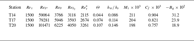
 Reδ∗=ρeueδ∗/μe
 Reθ=ρeueθ/μe
 Reδ2=ρeueθ/μw
 Reτ∗=ρeτwδ/μe
 Mτ=uτ/aw
 aw
 Cf=τw/(0.5ρeue2)
 Bq=qw/(ρwuτhw)
 τw=(μ∂u/∂y)|w
 qw=(−λ∂T/∂y)|w


 x
 z
 y∗≈40

 y∗≈40
 ρ¯/τwu″
 ρ¯R~T″/τw

 Reτ=1500

 Cf
 Cq
 Reδ∗

 Y+
 U+=Y+
 U+=1/0.41lnY++5.2

 M¯=|u|/a¯
 a
 y∗
 M=1

 T~/Te
 (T~−Tw)/Tw
 y∗
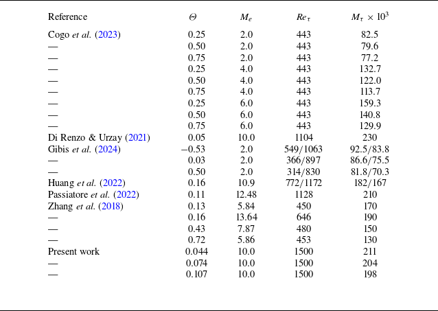

 y
 Θ

 Mt
 y∗

 y∗

 p′+=p′/τw
 y∗≈5
 θ′+=θ′μw/τw
 θ=∂ui/∂xi
 λx+=(2π/kx)/δv
 Ep′p′+=Ep′p′/τw2
 p′+
 z
 t
 y∗≈5
 z∗=z/δv∗
 t∗=t/(δv∗/uτ∗)

 y∗
 ρ¯uτ∗3
 uτ∗2/δv∗
 δy∗=(y∂h~/∂y=0∗−yρ¯h″v″~=0∗)/y∂h~/∂y=0∗
 Mτ

 ε=(h~DNS−h~DM)/h~DNS×100
 h~DM

 sPr


 N2
 O2
 y∗

 y∗


 N2
 O2
 y∗

 N2
 O2
 y∗
 μ¯/(ρ¯τw)

 N2
 O2
 y/δ99

 θ′/θrms′(y)
 −θ′/θrms′(y)

 Reτ=1500
 Δyw+
 Δyδ+
 y


 Open access

