1. Introduction
On 15 October 2000 an unintentional release of
 $150\,000\ \text{m}^{3}$
of water from Lac Inférieur, over a period of 20 h, caused a debris flow to form on the slope of Les Garette. This flowed downslope and arrived at the village of Fully, Switzerland as a sequence of 1–1.5 m thick surges, travelling at approximately
 $10\ \text{m}\ \text{s}^{-1}$
, which were interspersed by periods in which the remaining channel fill was completely stationary (Zanuttigh & Lamberti Reference Zanuttigh and Lamberti2007). Similar surges have been reported in the Jiang-Jia Ravine, China (Li et al.
Reference Li, Jianmo, Bi and Luo1983), Illgraben, Switzerland (McArdell et al.
Reference McArdell, Zanuttigh, Lamberti, Rickenmann, Rickenmann and Chen2003) and the Moscardo torrent, Italy (Marchi, Arattano & Deganutti Reference Marchi, Arattano and Deganutti2002). Although no one was hurt in Fully, it is important to understand how these surges form, because each pulse is much more destructive than a continuous flow of the same mass flux. Davies (Reference Davies1986) was perhaps the first to suggest that the most likely explanation for them was the spontaneous formation of roll waves (e.g. Cornish Reference Cornish1910; Dressler Reference Dressler1949; Needham & Merkin Reference Needham and Merkin1984; Kranenburg Reference Kranenburg1992; Balmforth & Liu Reference Balmforth and Liu2004; Balmforth & Mandre Reference Balmforth and Mandre2004; Zanuttigh & Lamberti Reference Zanuttigh and Lamberti2007), which merge and coarsen along the channel to form large-amplitude wave surges.
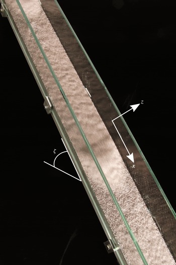
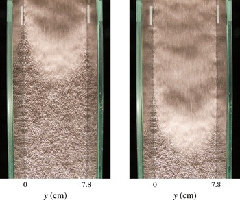
In this paper experiments are described that exhibit similar discrete surge-like behaviour in dry granular flows, albeit at a much smaller scale. Figure 1 shows a photograph of the chute, which is fed by a hopper with a steady supply of monodisperse carborundum grains. For slope inclinations just above the onset of flow, the free surface is unstable and small waves develop which grow in amplitude, merge and coarsen as they flow downslope. In many respects they initially look like granular roll waves (e.g. Davies Reference Davies1990; Vallance Reference Vallance1994; Forterre & Pouliquen Reference Forterre and Pouliquen2003; Forterre Reference Forterre2006; Iverson et al. Reference Iverson, Logan, LaHusen and Berti2010; Gray & Edwards Reference Gray and Edwards2014), but sufficiently far downstream the troughs, between the wave peaks, drop below the minimum thickness for flow and deposit material, which forms a stationary erodible layer between the thicker mobile parts of the waves. In the oblique view of the chute in figure 1 a long shutter speed is used to reveal the moving grains, which appear blurred, and the stationary regions, which are in sharp focus. A further two overhead photographs (figure 2), taken 0.4 s apart, show a close-up of the static layer ahead of the wave being eroded by the propagating wavefront. The major difference from conventional roll waves is therefore that completely stationary regions form spontaneously between the wave crests, which fundamentally change the nature of the solution. To make the distinction clear from the outset we therefore term them ‘erosion–deposition’ waves.
A photograph showing an oblique view of two erosion–deposition waves travelling down a chute inclined at
 ${\it\zeta}=35.1^{\circ }$
to the horizontal. The wavefronts appear brighter due to the lighting and a long time exposure has been used so that moving grains are blurred and the static regions are sharp. The chute has a total length of 3.29 m in the downslope
 $x$
direction, a width of 7.8 cm in the cross-slope
 $y$
direction and the glass sidewalls have a height of 6 cm in the
 $z$
direction normal to the plane. A movie showing the time-dependent evolution of the waves is available in the online supplementary material at http://dx.doi.org/10.1017/jfm.2014.643.

Two photographs of the experiment taken from a camera positioned above and normal to the chute, 0.4 s apart, showing a roll wave progressing downslope from the inflow end (top) to the outflow end (bottom). The material ahead of the mobile wavefront is the stationary deposit of a previous erosion–deposition wave. A movie showing the time-dependent evolution of the waves is available in the online supplementary material.

The surges, when viewed independently, resemble a solitary granular avalanche propagating on an erodible bed (see, e.g., Daerr & Douady Reference Daerr and Douady1999; Daerr Reference Daerr2001; Pouliquen & Forterre Reference Pouliquen and Forterre2002; Börzsönyi, Halsey & Ecke Reference Börzsönyi, Halsey and Ecke2005; Clement et al. Reference Clement, Malloggi, Andreotti and Aranson2007; Börzsönyi, Halsey & Ecke Reference Börzsönyi, Halsey and Ecke2008; Takagi, McElwaine & Huppert Reference Takagi, McElwaine and Huppert2011). We believe that each individual wave is directly related to the isolated triangular waves first reported in the literature by Daerr (Reference Daerr2001). Börzsönyi et al. (Reference Börzsönyi, Halsey and Ecke2005, Reference Börzsönyi, Halsey and Ecke2008) also observed these waves, which have a static layer ahead and behind of them, and postulated a simple Burgers-type equation for the evolving thickness. We have solved this equation numerically and found that an initial cap of material released on top of an erodible bed rapidly developed into a single triangular section of an N-wave (Whitham Reference Whitham1974). It is well known, however, that these decrease in height with increasing time, so this approach is not able to model steadily travelling solitary waves. Clement et al. (Reference Clement, Malloggi, Andreotti and Aranson2007) used Aranson & Tsimring’s (Reference Aranson and Tsimring2001, Reference Aranson and Tsimring2002) partial fluidization theory to construct a model consisting of a thin viscous film equation for the flow height and an order parameter for the fluidity, which was controlled by the Ginzburg–Landau equation. This model was able to generate solitary wave solutions, but really contains very little granular physics. Takagi et al. (Reference Takagi, McElwaine and Huppert2011) are the only ones to have reported multiple erosion–deposition waves, although these were generated by regular pile collapses at the source and did not interact with one another. The erosion–deposition waves reported here are therefore somewhat different, as they form spontaneously in a steady uniform flow and subsequently merge and coarsen very much like roll waves.
The theory developed in this paper builds on recent advances in modelling the constitutive behaviour of granular flows with the
 ${\it\mu}(I)$
-rheology (Jop, Forterre & Pouliquen Reference Jop, Forterre and Pouliquen2006). Numerical simulations using this rheology are now able to tackle complex flows, such as column collapses (Lagrée, Staron & Popinet Reference Lagrée, Staron and Popinet2011) and silos (Staron, Lagrée & Popinet Reference Staron, Lagrée and Popinet2012), but this is still challenging even in two dimensions. Conversely, one-dimensional depth-averaged avalanche models (Grigorian, Eglit & Iakimov Reference Grigorian, Eglit and Iakimov1967; Savage & Hutter Reference Savage and Hutter1989; Gray, Wieland & Hutter Reference Gray, Wieland and Hutter1999; Pouliquen Reference Pouliquen1999b
; Pouliquen & Forterre Reference Pouliquen and Forterre2002; Gray, Tai & Noelle Reference Gray, Tai and Noelle2003) have a much simpler description which has proven to be effective over many years. These are able to predict the critical Froude number for granular roll waves,
 $\mathit{Fr}_{c}>2/3$
, consistent with the experiments of Forterre & Pouliquen (Reference Forterre and Pouliquen2003), but incorrectly predict growth at all frequencies. Forterre (Reference Forterre2006) used linear stability analysis to show that the full
 ${\it\mu}(I)$
-rheology could predict the cutoff frequency, and attempted to depth-average the deviatoric stresses to derive a shallow-water-like system of equations that could also predict cutoff. This was only partially successful as the frequency could only be matched by adding an ad hoc fitting parameter. Gray & Edwards (Reference Gray and Edwards2014) recently developed a depth-averaged
 ${\it\mu}(I)$
-rheology that was able to match the cutoff frequency without any fitting parameters over a wide range of angles, i.e. without including ad hoc viscosity. In particular, the angle dependence provides strong evidence for its accuracy and it is this approach that is adopted here. Indeed, the viscous term plays a crucial role in modelling the erosion–deposition waves described in this paper.
2. Small-scale experiments
Laboratory experiments using
 $315{-}355\ {\rm\mu}\text{m}$
carborundum particles have been used to produce discrete surge waves similar to those observed in the October 2000 debris flow in Fully, Switzerland. The chute has glass sidewalls and the bed is roughened by attaching a monolayer of spherical glass beads of diameter
 $400{-}600\ {\rm\mu}\text{m}$
using double-sided sticky tape. It is inclined at
 ${\it\zeta}=35.1\pm 0.1^{\circ }$
to the horizontal and is supplied from the top by a perspex hopper with a double gate that allows the start time and inflow thickness to be controlled. The width of the chute is 7.8 cm and its length is 3.29 m from the inflow gate to the outflow, where the material flows out freely. A coordinate system
 $Oxyz$
is defined with the
 $x$
-axis pointing in the downslope direction, the
 $y$
-axis across the chute and the
 $z$
-axis pointing normal to the rough plane at
 $z=0$
. Experiments are initiated with a stationary layer of carborundum particles, deposited from a previous experiment, lining the bed. The flow is illuminated from the outflow end by a light source that is parallel to, and level with, the base. This creates bright areas in front of the wave peaks and shadows behind them, enhancing their appearance.
Data are acquired simultaneously using a combination of a camera, a scale and a laser profilometer. A high-speed camera (Teledyne DALSA Genie HM1400/HC1400) is used to capture still images of the flow normal to the chute from above, in a region between 2.21 and 3.29 m downslope of the inflow gate. At the outflow of the chute the material is collected in a tray on a high-resolution bench scale (KERN FKB 8K0.05) which outputs the measured mass to an accuracy of 50 mg at a rate of 5 Hz to a computer. A profilometer (Micro-Epsilon scanCONTROL 2700-100 laser profile sensor) is positioned with its laser line covering the width of the channel and perpendicular to the downslope direction, at a distance of
 $x_{L}=3.21\ \text{m}$
from the inflow gate. The profilometer measures the distance of the bulk flow particles away from the sensor, at a frequency of 100 Hz and to an accuracy of
 $\pm 0.2\ \text{mm}$
for a maximum of 40 s, by the method of laser line triangulation. Measurement of the distance of the bed from the sensor on the empty chute before or after an experiment allows the flow thickness profile
 $h$
along the laser line to be calculated.
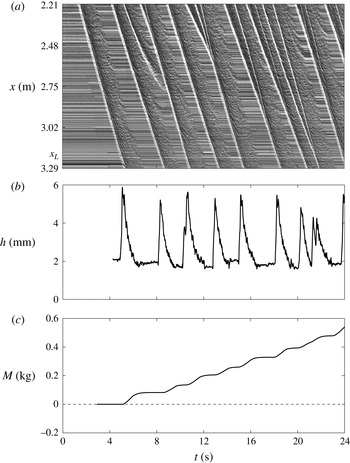
Experimental data for a period of 0–24 s. The space–time plot (a) is constructed by taking the middle column of each successive overhead still image and laying them out horizontally to give the downslope position
 $x$
with time
 $t$
. Horizontal lines indicate stationary grains and the wavefronts appear as diagonal white lines due to the illumination. Measurements from the laser profilometer (b) give the flow thickness
 $h$
on the centreline at
 $x=x_{L}=3.21\ \text{m}$
, which is near to the outflow. The balance data (c) give the accumulated mass
 $M$
that has flowed out of the chute.

The results from these three sources of data acquisition are shown for one run of the experiment in figure 3, for a time period of 0–24 s, where
 $t=0\ \text{s}$
is an arbitrarily chosen start time before the bulk flow reaches the region of interest (2.21–3.29 m from the inflow gate). The space–time plot in figure 3(a) is constructed by using the central column of pixels from each successive image. The wavefronts appear as bright lines, which are followed by darker regions behind the peak. The regions of horizontal lines indicate completely stationary grains between the surges. For an isolated erosion–deposition wave the wavefront and the boundary of the stationary region appear to be parallel straight lines, indicating that these are travelling waves moving at constant speed. All the waves have approximately the same speed, but there are several merging events, where they coalesce to form another travelling wave, such as at
 $t\approx 12\ \text{s}$
and
 $x\approx 2.48\ \text{m}$
in figure 3(a). Merging events are more frequent closer to the inflow gate. For this experiment the mean wavespeed is
 $u_{w}\approx 0.25\ \text{m}\ \text{s}^{-1}$
. The wave period, defined here as the time between successive wavefronts including the stationary regions, is found to have a mean value of
 $T\approx 2.36\ \text{s}$
and a corresponding frequency of
 $f\approx 0.42\ \text{Hz}$
. The wavelength including the static regions has a mean value of
 ${\it\lambda}\approx 0.59\ \text{m}$
.
The flow thickness profile
 $h$
on the centreline at
 $x=x_{L}=3.21\ \text{m}$
(near the end of the chute) is shown in figure 3(b). The thickness of the stationary regions between successive waves is defined as
 $h_{+}\approx 2.0\ \text{mm}$
and the maximum thickness at each roll wave peak is defined as
 $h_{w}\approx 5.2\ \text{mm}$
. This implies a mean wave amplitude of
 $A\approx 3.2\ \text{mm}$
for this experiment, where the amplitude is
 $$\begin{eqnarray}A=h_{w}-h_{+}.\end{eqnarray}$$
Figure 3(c) shows the accumulated mass at the end of the chute, which is a smooth increasing function of time. Regions with positive gradient correspond to the mobile part of the erosion–deposition waves reaching the outflow, whilst flat regions indicate that no grains are exiting the chute and correspond to the stationary regions between the surges. The discrete nature of the pulses that develop spontaneously from a steady uniform flow is a novel feature of the experiment.
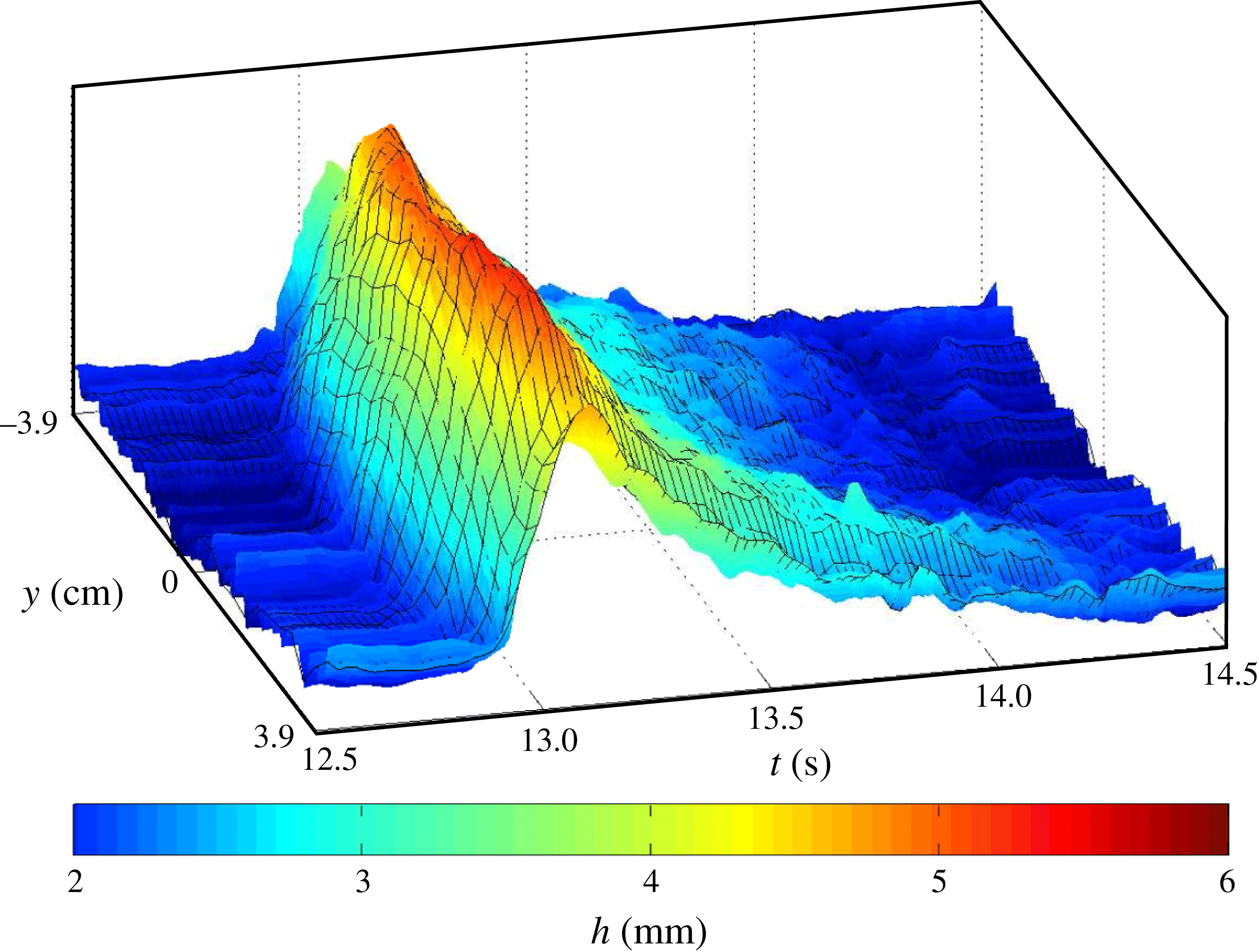
Measured variations in the shape of a single wave across the chute at
 $x=x_{L}$
are shown in the space–time plot in figure 4. This indicates that the thickness on the centreline is slightly higher and arrives slightly earlier than the material at the wall due to sidewall friction. This does not, however, appear to be a large effect. The depth of the static region is approximately the same before and after the passage of the wave and the variations in
 $h_{+}$
across the slope are of the order of the grain size.
A three-dimensional space–time plot of the free-surface height
 $h$
between
 $t=12.5$
and 14.5 s, for the experiment in figure 3, showing the variation of the wave in the cross-slope direction
 $y$
at
 $x=x_{L}=3.21\ \text{m}$
, where
 $y=0$
is the middle of the chute. A colour bar is used to show the height.

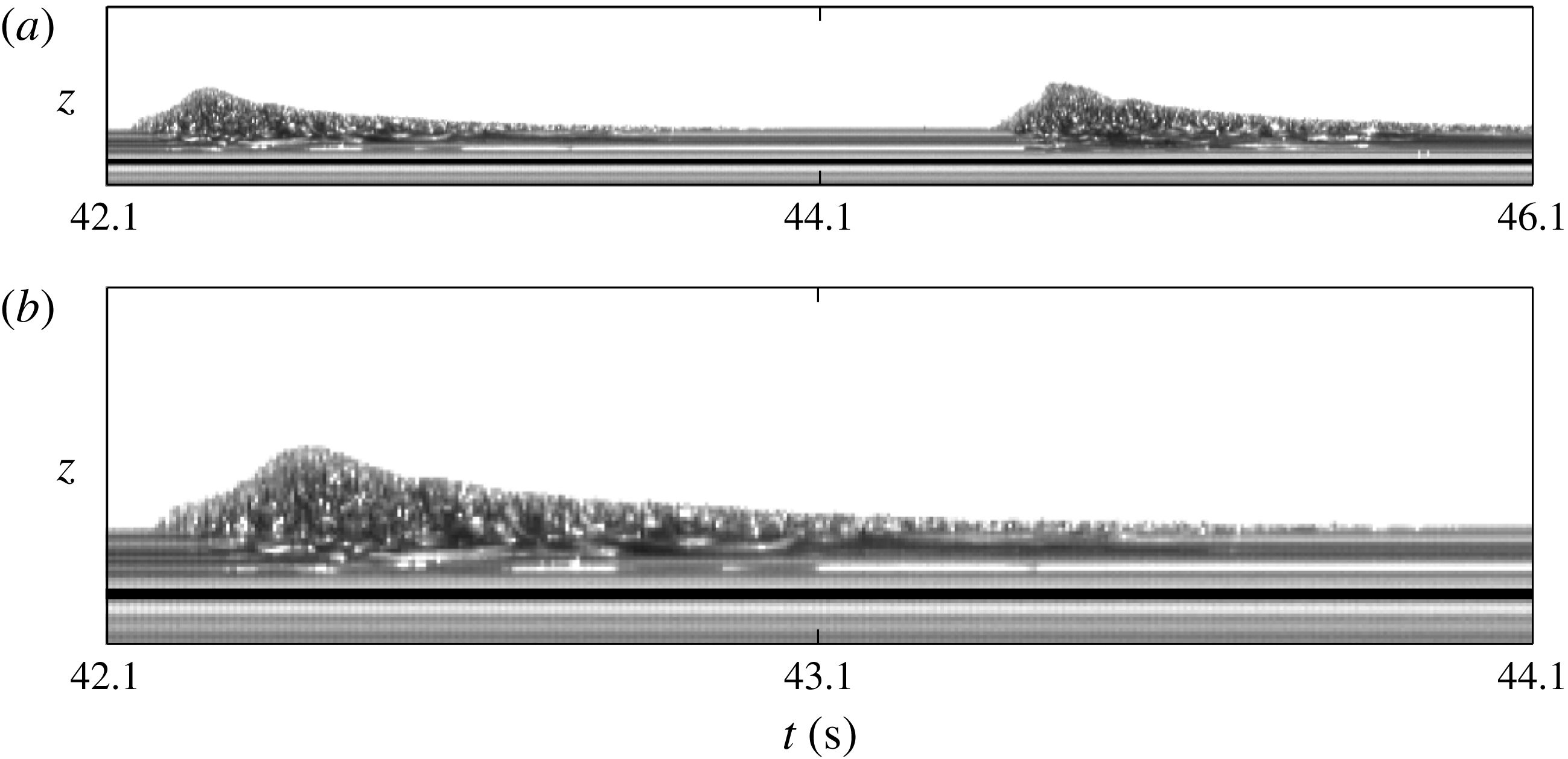
Space–time plots of the thickness profile of a flow of carborundum particles which is built from a sequence of images that view the flow through a glass sidewall and are aligned with the slope at a fixed
 $x$
position. The vertical axis gives the free-surface height and the horizontal axis gives the experiment time
 $t$
for a period of 4 s in (a) and 2 s in (b). The black line has been added to represent the position of the rough bed in relation to the bulk flow. Horizontal lines represent particles that are stationary and therefore show that particles come to rest between the wave surges. It should be noted that the flow front appears more diffuse than it actually is, because sidewall friction implies that the flow front in the centre is slightly in advance of that at the sidewall. A movie showing the time-dependent evolution of the waves through the sidewall is available in the online supplementary material.

The high-speed camera has also been positioned to one side of the chute and aligned with the slope angle
 ${\it\zeta}$
, so that the flow thickness profile past a point can be observed through the glass sidewalls. A space–time plot of the flow thickness profile in time is shown in figure 5 at a point 2.5 m downslope of the inflow gate. It shows how the erosion–deposition waves travel downslope by eroding the static layer of particles in front of them and depositing a static layer behind. When one of these waves is travelling steadily with a constant wavespeed, then the erosion–deposition process is in equilibrium. Interestingly, these plots show that the lowest point of particle motion is below the thickness of the static layers, but the erosion does not penetrate all the way down to the rough bed.
3. Governing equations
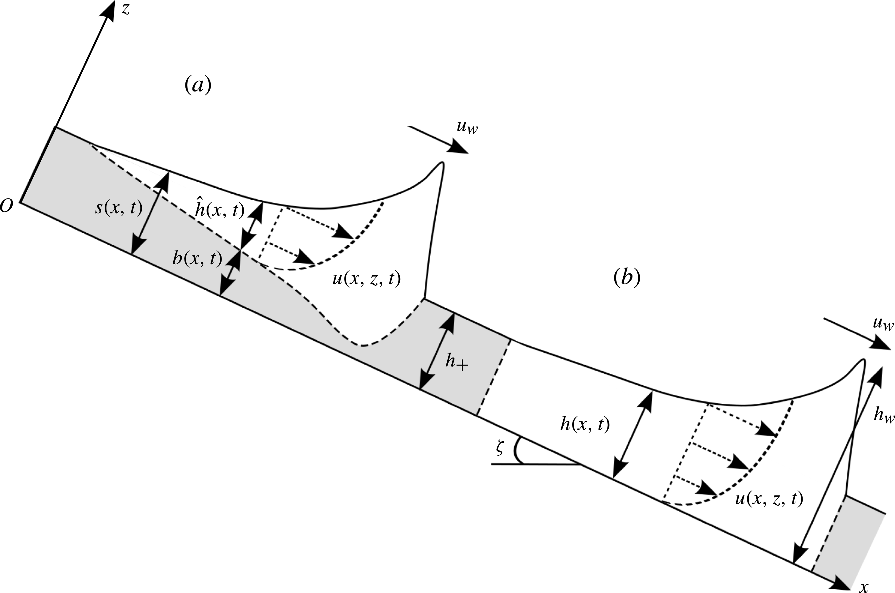
There are essentially two ways of modelling erosion–deposition waves within a depth-averaged framework, which are illustrated schematically in figure 6(a,b). In figure 6(a), the free surface lies at
 $z=s(x,t)$
, the interface between mobile and immobile regions lies at
 $z=b(x,t)$
and the difference,
 ${\hat{h}}=s-b$
, defines the avalanche depth. Modelling of flows using this approach is notoriously difficult, because an empirical/theoretical expression for the erosion/deposition rate,
 $d$
, at the base of the avalanche must be prescribed to close the system (e.g. Bouchaud et al.
Reference Bouchaud, Cates, Prakash and Edwards1994; Douady, Andreotti & Daerr Reference Douady, Andreotti and Daerr1999; Gray Reference Gray2001; Doyle et al.
Reference Doyle, Huppert, Lube, Mader and Sparks2007; Tai & Kuo Reference Tai and Kuo2008; Gray & Ancey Reference Gray and Ancey2009; Iverson Reference Iverson2012; Tai & Kuo Reference Tai and Kuo2012). However, in formulating the basal friction law that will be adopted in this paper, Pouliquen & Forterre (Reference Pouliquen and Forterre2002) implicitly assumed complete mobilization of particles throughout the entire depth, i.e. the flows were either completely mobile or completely static. While this is a crude approximation, it will be shown here that it allows considerable progress to be made. The free surface of the flow at
 $z=h(x,t)$
is therefore taken to be a measure of the flow thickness normal to the plane of both the mobile and the static regions of the particles, as shown in figure 6(b).
A schematic diagram showing two possible representations of an eroding and depositing granular avalanche on a slope inclined at an angle,
 ${\it\zeta}$
, to the horizontal. The stationary material is shaded grey. The flow thickness, in the normal
 $z$
direction, is considered to be either (a) the depth
 ${\hat{h}}(x,t)$
of particles between the free surface
 $s(x,t)$
and base of the avalanche at
 $z=b(x,t)$
, or (b) the entire depth
 $h(x,t)$
between the free surface and the bed. Typical downslope velocity profiles
 $u(x,z,t)$
through the depth of the flow are illustrated. The travelling-wave solution assumes that the wave moves with constant speed
 $u_{w}$
and erodes a static layer of grains of thickness
 $h_{+}$
ahead of the wave and deposits the same thickness behind it. The maximum height of the wave at the peak is denoted
 $h_{w}$
.

3.1. Depth-averaged equations with viscous dissipation
The avalanche is modelled using Gray & Edwards’s (Reference Gray and Edwards2014) theory, which is derived by depth-averaging the
 ${\it\mu}(I)$
-rheology (Jop et al.
Reference Jop, Forterre and Pouliquen2006) for dense granular flows. This model differs from standard shallow-water-type avalanche equations (Grigorian et al.
Reference Grigorian, Eglit and Iakimov1967; Savage & Hutter Reference Savage and Hutter1989; Gray et al.
Reference Gray, Wieland and Hutter1999; Pouliquen Reference Pouliquen1999b
; Pouliquen & Forterre Reference Pouliquen and Forterre2002; Gray et al.
Reference Gray, Tai and Noelle2003) by the inclusion of in-plane deviatoric normal stresses. For an avalanche of thickness
 $h$
and depth-averaged downslope velocity
 ${\bar{u}}$
the depth-averaged mass and momentum balance equations are
 $$\begin{eqnarray}\displaystyle & \displaystyle {\displaystyle \frac{\partial h}{\partial t}}+{\displaystyle \frac{\partial }{\partial x}}\left(h{\bar{u}}\right)=0, & \displaystyle\end{eqnarray}$$
 $$\begin{eqnarray}\displaystyle & \displaystyle {\displaystyle \frac{\partial }{\partial t}}\left(h{\bar{u}}\right)+{\displaystyle \frac{\partial }{\partial x}}\left({\it\chi}h{\bar{u}}^{2}\right)+{\displaystyle \frac{\partial }{\partial x}}\left(\frac{1}{2}h^{2}g\cos {\it\zeta}\right)=hgS+{\displaystyle \frac{\partial }{\partial x}}\left({\it\nu}h^{3/2}{\displaystyle \frac{\partial {\bar{u}}}{\partial x}}\right), & \displaystyle\end{eqnarray}$$
 ${\it\chi}=\overline{u^{2}}/{\bar{u}}^{2}$
is the shape factor and
 $g$
is the constant of gravitational acceleration. The
 ${\it\mu}(I)$
-rheology implies that for steady uniform flow a Bagnold velocity profile develops (see, e.g., GDR-MiDi 2004; Gray & Edwards Reference Gray and Edwards2014) and the resulting shape factor is
 ${\it\chi}=5/4$
. However, non-unity values of the shape factor change the characteristic structure of the inviscid equations, and cause problems when handling grain-free regions, so virtually all avalanche models (e.g. Grigorian et al.
Reference Grigorian, Eglit and Iakimov1967; Savage & Hutter Reference Savage and Hutter1989; Gray et al.
Reference Gray, Wieland and Hutter1999; Pouliquen Reference Pouliquen1999b
; Pouliquen & Forterre Reference Pouliquen and Forterre2002; Gray et al.
Reference Gray, Tai and Noelle2003) assume, as we do here, that
 ${\it\chi}=1$
. The source term,
 $$\begin{eqnarray}S=\sin {\it\zeta}-{\it\mu}{\displaystyle \frac{{\bar{u}}}{|{\bar{u}}|}}\cos {\it\zeta},\end{eqnarray}$$
consists of the component of gravity in the downslope
 $x$
direction and the effective basal friction
 ${\it\mu}$
between the avalanche and the rough plane, which opposes the direction of motion. The viscous term on the right-hand side of (3.2) plays a critical role in the formation of erosion–deposition waves. In their derivation, Gray & Edwards (Reference Gray and Edwards2014) showed that to leading order the
 ${\it\mu}(I)$
-rheology implies that there is a lithostatic pressure and a Bagnold velocity profile through the avalanche depth. To first order the shallow-water-like avalanche equations are recovered, with the only contributions from the
 ${\it\mu}(I)$
-rheology coming from the shape factor
 ${\it\chi}$
and an effective basal friction, which is equivalent to the dynamic friction law of Pouliquen & Forterre (Reference Pouliquen and Forterre2002) for Froude number
 $\mathit{Fr}>{\it\beta}$
. Similar equations have been used for many years (e.g. Grigorian et al.
Reference Grigorian, Eglit and Iakimov1967; Pouliquen Reference Pouliquen1999b
; Gray et al.
Reference Gray, Tai and Noelle2003) and are sufficient for many applications (e.g. Johnson & Gray Reference Johnson and Gray2011; Cui & Gray Reference Cui and Gray2013). However, they are unable to predict the cutoff frequency of roll waves (Forterre & Pouliquen Reference Forterre and Pouliquen2003).
Extension to second order leads to very complicated models that are often difficult to interpret. Gray & Edwards (Reference Gray and Edwards2014) therefore used a pragmatic approach, in which they included the depth-averaged in-plane deviatoric stress in (3.2). This was evaluated by substituting the lithostatic pressure and Bagnold velocity into the
 ${\it\mu}(I)$
-rheology (Jop et al.
Reference Jop, Forterre and Pouliquen2006) and integrating. They then used the leading-order relationship between the depth-averaged Bagnold velocity and the thickness to reformulate the result into the viscous-like term, where other contributions with lower-order gradients were neglected, since they do not contribute to the principal part. At this order, the leading-order balance can be used to create many different formulations. The one given in (3.2) has been specifically chosen because for angles in the steady uniform regime it does not introduce any singularities and it degenerates in grain-free regions. The coefficient
 $$\begin{eqnarray}{\it\nu}=\frac{2}{9}\frac{\mathscr{L}\sqrt{g}}{{\it\beta}}\frac{\sin {\it\zeta}}{\sqrt{\cos {\it\zeta}}}\left(\frac{\tan {\it\zeta}_{2}-\tan {\it\zeta}}{\tan {\it\zeta}-\tan {\it\zeta}_{1}}\right),\end{eqnarray}$$
where
 $\mathscr{L}$
and
 ${\it\beta}$
, and the angles
 ${\it\zeta}_{1}$
and
 ${\it\zeta}_{2}$
arise directly from Pouliquen & Forterre’s (Reference Pouliquen and Forterre2002) basal friction law, which will be described in greater detail below. It should be noted that the Gray & Edwards (Reference Gray and Edwards2014) theory is only well-posed for angles
 ${\it\zeta}_{1}\leqslant {\it\zeta}\leqslant {\it\zeta}_{2}$
. This is a signature of the ill-posedness of the
 ${\it\mu}(I)$
-rheology for both high and low inertial numbers (Barker et al.
Reference Barker, Schaeffer, Bohórquez and Gray2014). The inclusion of the viscous term represents a singular perturbation to the problem. Most of the time it is negligibly small, but sometimes it plays a critical role, which proves to be the case for the erosion–deposition waves studied here. Strong evidence for this theory and the specific angle dependence in (3.4) is provided by the fact that Gray & Edwards (Reference Gray and Edwards2014) were able to match the experimental cutoff frequency for roll waves (Forterre & Pouliquen Reference Forterre and Pouliquen2003) over a wide range of angles without any fitting parameters. The viscous term in (3.2) therefore has a strong physical basis rather than being just an ad hoc regularization with an unspecified coefficient of viscosity.
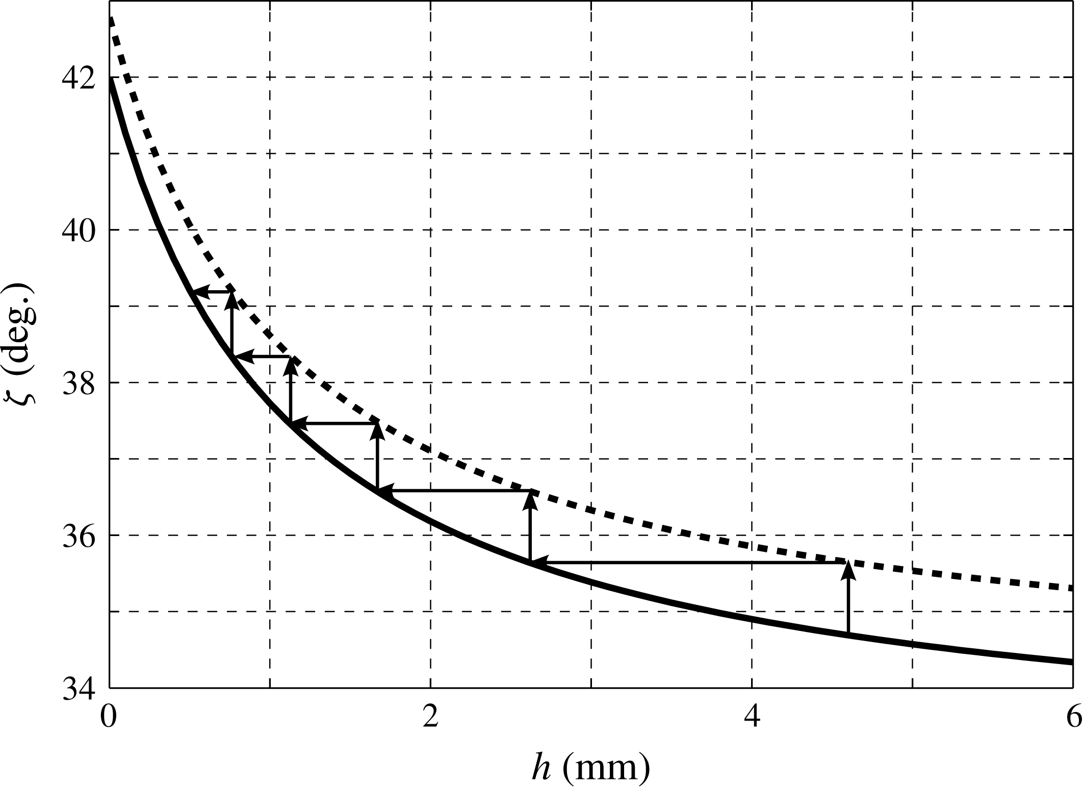
Critical angle curves
 ${\it\zeta}_{stop}$
(solid line) and
 ${\it\zeta}_{start}$
(dashed line) as functions of the flow thickness. The plot is annotated with arrows to show the progression between the curves as they are found experimentally (see Pouliquen & Forterre Reference Pouliquen and Forterre2002) by increasing the slope angle to trigger avalanches that leave deposits of decreasing thickness.

3.2. Pouliquen and Forterre’s basal friction law
The basal friction law also plays a pivotal part in allowing flows like those observed experimentally to be modelled by a framework that does not explicitly include the effects of erosion and deposition. Pouliquen (Reference Pouliquen1999a
) performed laboratory experiments on flows of spherical glass beads on a rough chute and found an empirical friction law that was valid for steady uniform flows at various slope angles. An extension of this by Pouliquen & Forterre (Reference Pouliquen and Forterre2002) found two critical slope inclination angles as functions of the flow thickness, namely
 ${\it\zeta}_{stop}(h)$
and
 ${\it\zeta}_{start}(h)$
. The function
 ${\it\zeta}_{stop}(h)$
gives the slope angle at which a steady uniform flow leaves a deposit of thickness
 $h$
, while
 ${\it\zeta}_{start}(h)$
is the angle at which a layer of thickness
 $h$
is mobilized. The two functions are illustrated in figure 7 for the parameters given in table 1, together with arrows to indicate a typical sequence of avalanches that they used to determine them. At a given thickness
 $h_{1}$
, the inclination angle is increased until a layer of static grains is mobilized, which determines
 ${\it\zeta}_{start}(h_{1})$
, after which the avalanche thickness decreases until the layer stops, determining
 ${\it\zeta}_{stop}(h_{2})$
at a new thickness
 $h_{2}$
. This behaviour is also observed for flows of various particle types and bed roughness conditions (e.g. Pouliquen & Renaut Reference Pouliquen and Renaut1996; Daerr & Douady Reference Daerr and Douady1999).
Material properties.

The thickness of a deposit left by a steady uniform flow at an inclination angle
 ${\it\zeta}$
is denoted by
 $h_{stop}({\it\zeta})$
, which is the inverse function of
 ${\it\zeta}_{stop}(h)$
. An empirical dependence was found by Pouliquen (Reference Pouliquen1999a
) between the ratio of the flow thickness
 $h$
to
 $h_{stop}({\it\zeta})$
and the Froude number,
 $\mathit{Fr}={\bar{u}}/\sqrt{hg\cos {\it\zeta}}$
, which is given here as
 $$\begin{eqnarray}\mathit{Fr}={\it\beta}\frac{h}{h_{stop}({\it\zeta})}.\end{eqnarray}$$
The constant is
 ${\it\beta}=0.136$
for spherical glass beads and 0.65 for sand on a rough bed of the same material (Forterre & Pouliquen Reference Forterre and Pouliquen2003). It should be noted that Forterre & Pouliquen (Reference Forterre and Pouliquen2003) found that there was also an offset at the origin for sand in (3.5). Although this is very easy to programme into the basal friction law, it is unclear how to include it into the
 ${\it\mu}(I)$
-rheology, since it is no longer possible to use Jop, Forterre & Pouliquen’s (Reference Jop, Forterre and Pouliquen2005) method of inferring the rheology from the basal friction law. The offset is therefore neglected in this paper, although the value of
 ${\it\beta}=0.65$
for sand is used to approximate the friction of our carborundum particles flowing on a rough bed of spherical glass beads. One consequence of using the simpler law (3.5) is that, in principle, it should be possible to observe erosion–deposition waves for all forms of particles, including ballotini, although the region of parameter space where this occurs may be small.
For steady uniform flows the depth-averaged momentum balance (3.2) is satisfied provided the source terms are identically zero, which implies that
 $$\begin{eqnarray}{\it\mu}=\tan {\it\zeta}.\end{eqnarray}$$
By defining the tangent of the critical stopping angle as
 $$\begin{eqnarray}{\it\mu}_{stop}(h)=\tan ({\it\zeta}_{stop}(h)),\end{eqnarray}$$
the friction coefficient for the static layer is found through the steady uniform flow relation (3.6) and the empirical law (3.5) to be
 $$\begin{eqnarray}{\it\mu}=\tan {\it\zeta}=\tan ({\it\zeta}_{stop}(h_{stop}({\it\zeta})))={\it\mu}_{stop}(h_{stop}({\it\zeta}))={\it\mu}_{stop}\left(\frac{h{\it\beta}}{\mathit{Fr}}\right).\end{eqnarray}$$
However, the empirical law (3.5), and therefore the friction law (3.8), is only valid for flows in the steady regime,
 $h\geqslant h_{stop}({\it\zeta})$
, or equivalently for flows in which
 $\mathit{Fr}\geqslant {\it\beta}$
. Defining the tangent of the critical starting angle as
 $$\begin{eqnarray}{\it\mu}_{start}(h)=\tan ({\it\zeta}_{start}(h)),\end{eqnarray}$$
Pouliquen & Forterre (Reference Pouliquen and Forterre2002) showed that a knowledge of the functions
 ${\it\mu}_{stop}(h)$
and
 ${\it\mu}_{start}(h)$
is sufficient to define an empirical friction law,
 ${\it\mu}(h,\mathit{Fr})$
, for the whole range of possible flow thicknesses and Froude numbers. The static friction coefficient, which holds for
 $\mathit{Fr}=0$
, is defined as
 $$\begin{eqnarray}{\it\mu}(h,0)=\tan ({\it\zeta}_{start}(h))={\it\mu}_{start}(h),\end{eqnarray}$$
since for stationary material the basal friction must balance the lithostatic pressure and gravitational forces exactly, so that the source terms balance and (3.6) still holds. In the intermediate friction regime when
 $0<\mathit{Fr}<{\it\beta}$
, the friction coefficient
 ${\it\mu}$
is given by a power law extrapolation between the friction laws in the static and dynamic friction regimes as
 $$\begin{eqnarray}{\it\mu}(h,\mathit{Fr})=\left({\displaystyle \frac{\mathit{Fr}}{{\it\beta}}}\right)^{{\it\kappa}}({\it\mu}_{stop}(h)-{\it\mu}_{start}(h))+{\it\mu}_{start}(h),\end{eqnarray}$$
where
 ${\it\kappa}=10^{-3}$
is the power of the extrapolation chosen by Pouliquen & Forterre (Reference Pouliquen and Forterre2002). The forms of the functions
 ${\it\mu}_{stop}$
and
 ${\it\mu}_{start}$
are given by fits to experimental measurements as transitions between the relevant critical friction angles. They are written here as
 $$\begin{eqnarray}{\it\mu}_{stop}(H)=\tan {\it\zeta}_{1}+\frac{\tan {\it\zeta}_{2}-\tan {\it\zeta}_{1}}{1+H/\mathscr{L}}\end{eqnarray}$$
and
 $$\begin{eqnarray}{\it\mu}_{start}(h)=\tan {\it\zeta}_{3}+\frac{\tan {\it\zeta}_{2}-\tan {\it\zeta}_{1}}{1+h/\mathscr{L}},\end{eqnarray}$$
where the dummy variable,
 $H=h{\it\beta}/\mathit{Fr}$
or
 $H=h$
, is dependent on where
 ${\it\mu}_{stop}$
is to be evaluated (i.e. for
 $\mathit{Fr}\geqslant {\it\beta}$
or
 $0<\mathit{Fr}<{\it\beta}$
respectively). There is no flow for inclination angles
 ${\it\zeta}<{\it\zeta}_{1}$
, which is the asymptote of the curve
 ${\it\zeta}_{stop}(h)$
for large
 $h$
, and the flow is accelerated for
 ${\it\zeta}>{\it\zeta}_{2}={\it\zeta}_{stop}(0)$
. The third critical angle,
 ${\it\zeta}_{3}$
, is the asymptote of the curve
 ${\it\zeta}_{start}(h)$
for large
 $h$
. The parameter
 $\mathscr{L}$
(having the dimensions of a length) is the characteristic depth of flow over which a transition between the angles
 ${\it\zeta}_{1}$
and
 ${\it\zeta}_{2}$
occurs, and as such it is dependent on the properties of the grains and on the bed roughness. In summary, the friction coefficient can be written in each of the three flow regimes, which will be referred to as dynamic, intermediate and static respectively, as
 $$\begin{eqnarray}\displaystyle & {\it\mu}(h,\mathit{Fr})={\it\mu}_{1}+\displaystyle \frac{{\it\mu}_{2}-{\it\mu}_{1}}{1+h{\it\beta}/(\mathscr{L}\mathit{Fr})},\quad \mathit{Fr}\geqslant {\it\beta}, & \displaystyle\end{eqnarray}$$
 $$\begin{eqnarray}\displaystyle & {\it\mu}(h,\mathit{Fr})=\left({\displaystyle \frac{\mathit{Fr}}{{\it\beta}}}\right)^{{\it\kappa}}({\it\mu}_{1}-{\it\mu}_{3})+{\it\mu}_{3}+\displaystyle \frac{{\it\mu}_{2}-{\it\mu}_{1}}{1+h/\mathscr{L}},\quad 0<\mathit{Fr}<{\it\beta}, & \displaystyle\end{eqnarray}$$
 $$\begin{eqnarray}\displaystyle & {\it\mu}(h,\mathit{Fr})={\it\mu}_{3}+\displaystyle \frac{{\it\mu}_{2}-{\it\mu}_{1}}{1+h/\mathscr{L}},\quad \mathit{Fr}=0, & \displaystyle\end{eqnarray}$$
 ${\it\mu}_{1}=\tan {\it\zeta}_{1}$
,
 ${\it\mu}_{2}=\tan {\it\zeta}_{2}$
and
 ${\it\mu}_{3}=\tan {\it\zeta}_{3}$
are the tangents of the critical angles,
 ${\it\zeta}_{1}$
,
 ${\it\zeta}_{2}$
and
 ${\it\zeta}_{3}$
. Values of the friction angles,
 ${\it\zeta}_{i}\ (i=1\dots 3)$
, along with the parameters,
 ${\it\beta}$
and
 $\mathscr{L}$
, are estimated for the experimental set-up of § 2. They are given in table 1, together with the exact experimental slope angle,
 ${\it\zeta}$
, and the resultant value of the effective viscosity,
 ${\it\nu}$
. These values remain fixed throughout this paper. It should be noted that Gray & Edwards’ (Reference Gray and Edwards2014) derivation of the viscous term in (3.2) implicitly assumes that the friction law is always given by the dynamic case (3.14). In principle, the form of the viscous term should change when the friction law is in the intermediate or static regime, i.e. for
 $\mathit{Fr}<{\it\beta}$
. However, it is not obvious how to achieve this, since there is no longer a steady uniform flow solution to determine the velocity and pressure profiles in the depth integration process. For simplicity, in this paper it is therefore assumed that the simple viscous term in (3.2) applies over all regimes.
4. Travelling erosion–deposition waves
Travelling-wave solutions to the depth-averaged mass and momentum conservation laws (3.1) and (3.2) are sought for an erosion–deposition wave moving downslope with speed
 $u_{w}$
. A wavefront-centred coordinate system,
 $({\it\xi},{\it\tau})$
, is introduced by the transformation
 $$\begin{eqnarray}{\it\xi}=x-u_{w}t,\quad {\it\tau}=t.\end{eqnarray}$$
Assuming a steady solution in the moving frame by setting
 $\partial /\partial {\it\tau}=0$
, the system is reduced to a pair of ordinary differential equations (ODEs),
 $$\begin{eqnarray}\displaystyle & \displaystyle {\displaystyle \frac{\text{d}}{\text{d}{\it\xi}}}\left(h({\bar{u}}-u_{w})\right)=0, & \displaystyle\end{eqnarray}$$
 $$\begin{eqnarray}\displaystyle & \displaystyle h({\bar{u}}-u_{w}){\displaystyle \frac{\text{d}{\bar{u}}}{\text{d}{\it\xi}}}+hg\cos {\it\zeta}{\displaystyle \frac{\text{d}h}{\text{d}{\it\xi}}}=hg\cos {\it\zeta}(\tan {\it\zeta}-{\it\mu})+{\displaystyle \frac{\text{d}}{\text{d}{\it\xi}}}\left({\it\nu}h^{3/2}{\displaystyle \frac{\text{d}{\bar{u}}}{\text{d}{\it\xi}}}\right), & \displaystyle\end{eqnarray}$$
 ${\bar{u}}/|{\bar{u}}|=1$
everywhere and the friction coefficient
 ${\it\mu}={\it\mu}(h,\mathit{Fr})$
is given by (3.14)–(3.16). The mass balance equation can be integrated immediately, subject to the condition that
 ${\bar{u}}=0$
in a stationary layer of thickness
 $h=h_{+}$
, to show that
 $$\begin{eqnarray}h({\bar{u}}-u_{w})=-h_{+}u_{w},\end{eqnarray}$$
which implies that the depth-averaged velocity is
 $$\begin{eqnarray}{\bar{u}}=u_{w}\left(1-\frac{h_{+}}{h}\right).\end{eqnarray}$$
Substitution of (4.5) into the momentum balance (4.3) yields a second-order ODE for
 $h$
,
 $$\begin{eqnarray}{\displaystyle \frac{\text{d}^{2}h}{\text{d}{\it\xi}^{2}}}=\frac{1}{2h}\left({\displaystyle \frac{\text{d}h}{\text{d}{\it\xi}}}\right)^{2}+\frac{h^{3/2}g\cos {\it\zeta}}{{\it\nu}h_{+}u_{w}}\left[\left(1-\frac{h_{+}^{2}u_{w}^{2}}{h^{3}g\cos {\it\zeta}}\right){\displaystyle \frac{\text{d}h}{\text{d}{\it\xi}}}-\tan {\it\zeta}+{\it\mu}\right],\end{eqnarray}$$
which determines the thickness profile of a travelling-wave solution with erosion and deposition. This ODE looks similar to the one that governs roll waves (see, e.g., Gray & Edwards Reference Gray and Edwards2014), but the fact that the velocity (4.5) equals zero, when
 $h=h_{+}$
, fundamentally changes the structure of the solutions. It is this distinction that has led to the introduction of the new terminology of an ‘erosion–deposition’ wave.
In (4.6) the friction coefficient,
 ${\it\mu}={\it\mu}(h,\mathit{Fr})$
, transitions between three different expressions, (3.14)–(3.16), dependent on whether
 $\mathit{Fr}\geqslant {\it\beta}$
,
 ${\it\beta}>\mathit{Fr}>0$
or
 $\mathit{Fr}=0$
. For steady uniform flows, Pouliquen’s (Reference Pouliquen1999a
) empirical law (3.5) implies that
 $h=h_{stop}({\it\zeta})$
when
 $\mathit{Fr}={\it\beta}$
. An explicit expression for
 $h_{stop}({\it\zeta})$
is found by substituting (3.14) into (3.6) and setting
 $\mathit{Fr}={\it\beta}$
to give
 $$\begin{eqnarray}h_{stop}({\it\zeta})=\mathscr{L}{\it\gamma},\end{eqnarray}$$
where
 $$\begin{eqnarray}{\it\gamma}=\frac{\tan {\it\zeta}_{2}-\tan {\it\zeta}_{1}}{\tan {\it\zeta}-\tan {\it\zeta}_{1}}-1\end{eqnarray}$$
is dependent on the inclination
 ${\it\zeta}$
. For the values of the parameters used here (table 1) the constant
 ${\it\gamma}\approx 3.5358$
and
 $h_{stop}\approx 3.5358\ \text{mm}$
. It is not, however, true that
 $\mathit{Fr}={\it\beta}$
at
 $h=h_{stop}({\it\zeta})$
for non-uniform flows, such as for the travelling-wave solutions that are being sought here. The actual flow thickness for which
 $\mathit{Fr}={\it\beta}$
is now defined as
 $h=h_{\star }$
, where
 $h_{\star }\neq h_{stop}$
must be solved for as part of the problem. It follows that the friction law varies in three regions in which
 $h\geqslant h_{\star }$
,
 $h_{\star }>h>h_{+}$
or
 $h=h_{+}$
, corresponding to where
 $\mathit{Fr}\geqslant {\it\beta}$
,
 ${\it\beta}>\mathit{Fr}>0$
or
 $\mathit{Fr}=0$
, respectively.
For the travelling wave the Froude number can be expressed solely in terms of the flow thickness
 $h$
, by substituting the depth-averaged velocity (4.5) into
 $\mathit{Fr}={\bar{u}}/\sqrt{hg\cos {\it\zeta}}$
to give
 $$\begin{eqnarray}\mathit{Fr}(h)=\frac{u_{w}(h-h_{+})}{h^{3/2}\sqrt{g\cos {\it\zeta}}}.\end{eqnarray}$$
A Froude number equal to
 ${\it\beta}$
now corresponds to a flow thickness of
 $h_{\star }$
, by definition, and so equating (4.9) to
 ${\it\beta}$
when
 $h=h_{\star }$
gives the propagation speed of the travelling wave,
 $$\begin{eqnarray}u_{w}=\frac{{\it\beta}h_{\star }^{3/2}\sqrt{g\cos {\it\zeta}}}{h_{\star }-h_{+}}.\end{eqnarray}$$
The Froude number may then be expressed independently of the wavespeed
 $u_{w}$
by substituting (4.10) into (4.9) to give
 $$\begin{eqnarray}\mathit{Fr}(h)=\frac{{\it\beta}h_{\star }^{3/2}(h-h_{+})}{h^{3/2}(h_{\star }-h_{+})},\end{eqnarray}$$
which is dependent on the parameters
 $h_{\star }$
,
 $h_{+}$
and the known constant
 ${\it\beta}$
. Substitution of (4.11) into (3.14)–(3.16) allows the friction law to be expressed purely as a function of thickness,
 $h$
, i.e.
 $$\begin{eqnarray}\displaystyle & \displaystyle {\it\mu}(h)={\it\mu}_{1}+\displaystyle \frac{{\it\mu}_{2}-{\it\mu}_{1}}{1+{\displaystyle \frac{h^{5/2}(h_{\star }-h_{+})}{\mathscr{L}h_{\star }^{3/2}(h-h_{+})}}},\quad h_{\star }\leqslant h, & \displaystyle\end{eqnarray}$$
 $$\begin{eqnarray}\displaystyle & \displaystyle {\it\mu}(h)=\left(\displaystyle \frac{h_{\star }^{3/2}(h-h_{+})}{h^{3/2}(h_{\star }-h_{+})}\right)^{{\it\kappa}}({\it\mu}_{1}-{\it\mu}_{3})+{\it\mu}_{3}+\displaystyle \frac{{\it\mu}_{2}-{\it\mu}_{1}}{1+h/\mathscr{L}},\quad h_{+}<h<h_{\star }, & \displaystyle\end{eqnarray}$$
 $$\begin{eqnarray}\displaystyle & \displaystyle {\it\mu}(h)={\it\mu}_{3}+\displaystyle \frac{{\it\mu}_{2}-{\it\mu}_{1}}{1+h/\mathscr{L}},\quad h=h_{+}. & \displaystyle\end{eqnarray}$$
4.1. Initial value problem
The second-order ODE (4.6) is solved numerically using MATLAB’s ode45 initial value problem solver by writing the equation as a pair of first-order ODEs. The first of these is the definition of a new variable,
 $n$
, as
 $$\begin{eqnarray}{\displaystyle \frac{\text{d}h}{\text{d}{\it\xi}}}=n,\end{eqnarray}$$
and the latter is obtained by substituting the wavespeed (4.10) into (4.6) and writing it in terms of
 $h$
and
 $n$
to give
 $$\begin{eqnarray}{\displaystyle \frac{\text{d}n}{\text{d}{\it\xi}}}=\frac{n^{2}}{2h}+\frac{\sqrt{g\cos {\it\zeta}}(h_{\star }-h_{+})h^{3/2}}{{\it\beta}{\it\nu}h_{\star }^{3/2}h_{+}}\left[\left(1-\frac{{\it\beta}^{2}h_{\star }^{3}h_{+}^{2}}{(h_{\star }-h_{+})^{2}h^{3}}\right)n-\tan {\it\zeta}+{\it\mu}(h)\right].\end{eqnarray}$$
The pair of coupled ODEs (4.15) and (4.16) are solved for
 $h$
and
 $n$
in the mobile section of the wave for a prescribed value of
 $h_{\star }$
. The solution is started from the rear of the wave located at
 ${\it\xi}=0$
(chosen arbitrarily) where the depth of the static region is assumed to be
 $h_{+}$
and the thickness gradient is zero, i.e.
 $$\begin{eqnarray}h({\it\xi}=0)=h_{+},\quad n({\it\xi}=0)=0.\end{eqnarray}$$
For each value of the thickness
 $h_{\star }$
there is a unique value of
 $h_{+}$
that enables the static layer to be the same thickness at the front and rear of the wave. The value of
 $h_{+}\in [0,h_{stop}]$
is found iteratively for each
 $h_{\star }$
by imposing the condition that
 $$\begin{eqnarray}h({\it\xi}={\it\Lambda})=h_{+},\quad n({\it\xi}={\it\Lambda})=0,\end{eqnarray}$$
at the front,
 ${\it\xi}={\it\Lambda}$
. The wavelength
 ${\it\Lambda}$
of the mobile section of the wave is a result of the integration, rather than being specified, and the static regions on either side can be of arbitrary length. Once
 $h_{\star }$
and
 $h_{+}$
are known the wavespeed
 $u_{w}$
is recovered from (4.10) and the depth-averaged velocity is given by (4.5).
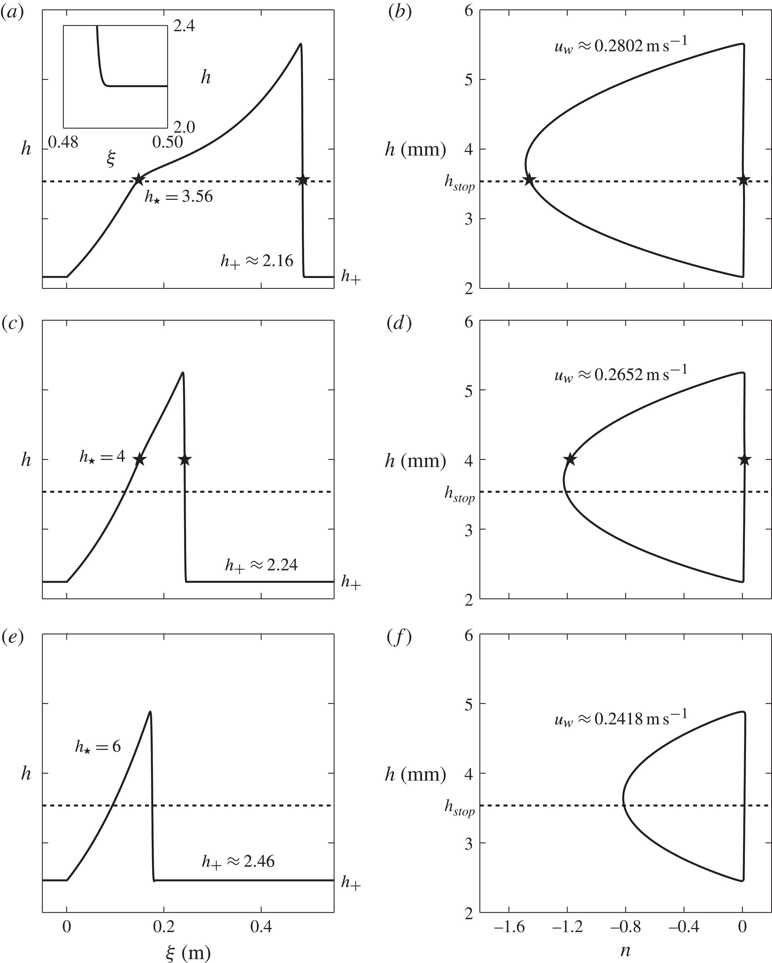
Three typical solutions in the physical domain,
 $({\it\xi},h)$
(for
 $-0.05\ \text{m}\leqslant {\it\xi}\leqslant 0.55\ \text{m}$
), and phase plane,
 $(n,h)$
, are shown in figure 8 for the following pairs of the input parameters,
 $h_{\star }$
and the corresponding, iteratively determined,
 $h_{+}$
:
 $$\begin{eqnarray}\text{Figure 8}(\mathit{a,b})\text{:}\quad h_{\star }=3.56\ \text{mm},\quad h_{+}\approx 2.16\ \text{mm},\end{eqnarray}$$
 $$\begin{eqnarray}\text{Figure 8}(\mathit{c,d})\text{:}\quad h_{\star }=4.00\ \text{mm},\quad h_{+}\approx 2.24\ \text{mm},\end{eqnarray}$$
 $$\begin{eqnarray}\text{Figure 8}(\mathit{e,f})\text{:}\quad h_{\star }=6.00\ \text{mm},\quad h_{+}\approx 2.46\ \text{mm}.\end{eqnarray}$$
All of the waves appear to have a shock at the front and a finite gradient at the rear, but, as the inset in figure 8(a) shows, the transitions to the static layer are continuous. It is very surprising that despite the inclusion of depth-averaged viscous dissipation in the momentum balance (3.2) a finite-length mobile wave arises naturally from the equations. The solutions generated here are therefore also able to explain the isolated triangular solitary waves observed on erodible beds (Daerr Reference Daerr2001; Börzsönyi et al. Reference Börzsönyi, Halsey and Ecke2005; Clement et al. Reference Clement, Malloggi, Andreotti and Aranson2007; Börzsönyi et al. Reference Börzsönyi, Halsey and Ecke2008; Takagi et al. Reference Takagi, McElwaine and Huppert2011) as well as the multiple erosion–deposition waves that spontaneously form from a steady uniform flow detailed in § 2. There are two types of solution: (i) ones in which all the friction regimes are activated (shown in (a,c)) and (ii) those where the mobile section of the wave is entirely in the intermediate friction regime (e).
Typical travelling-wave solutions (solid lines) to the coupled ODEs (4.15) and (4.16) showing how the flow thickness
 $h$
varies with downslope position
 ${\it\xi}$
(a,c,e) and
 $n=\text{d}h/\text{d}{\it\xi}$
(b,d, f). Each solution corresponds to a pair of input parameters
 $h_{\star }$
(star marker) and
 $h_{+}$
(thickness of constant/stationary layer) which are given in (4.19) for (a,b), (4.20) for (c,d) and (4.21) for (e, f). The minimum value of the input parameter
 $h_{\star }$
is
 $h_{stop}$
(dashed line). The wavespeed is determined from each
 $(h_{+},h_{\star })$
pair by (4.10). The inset in (a) shows the smooth transition to zero gradient over a finite length.

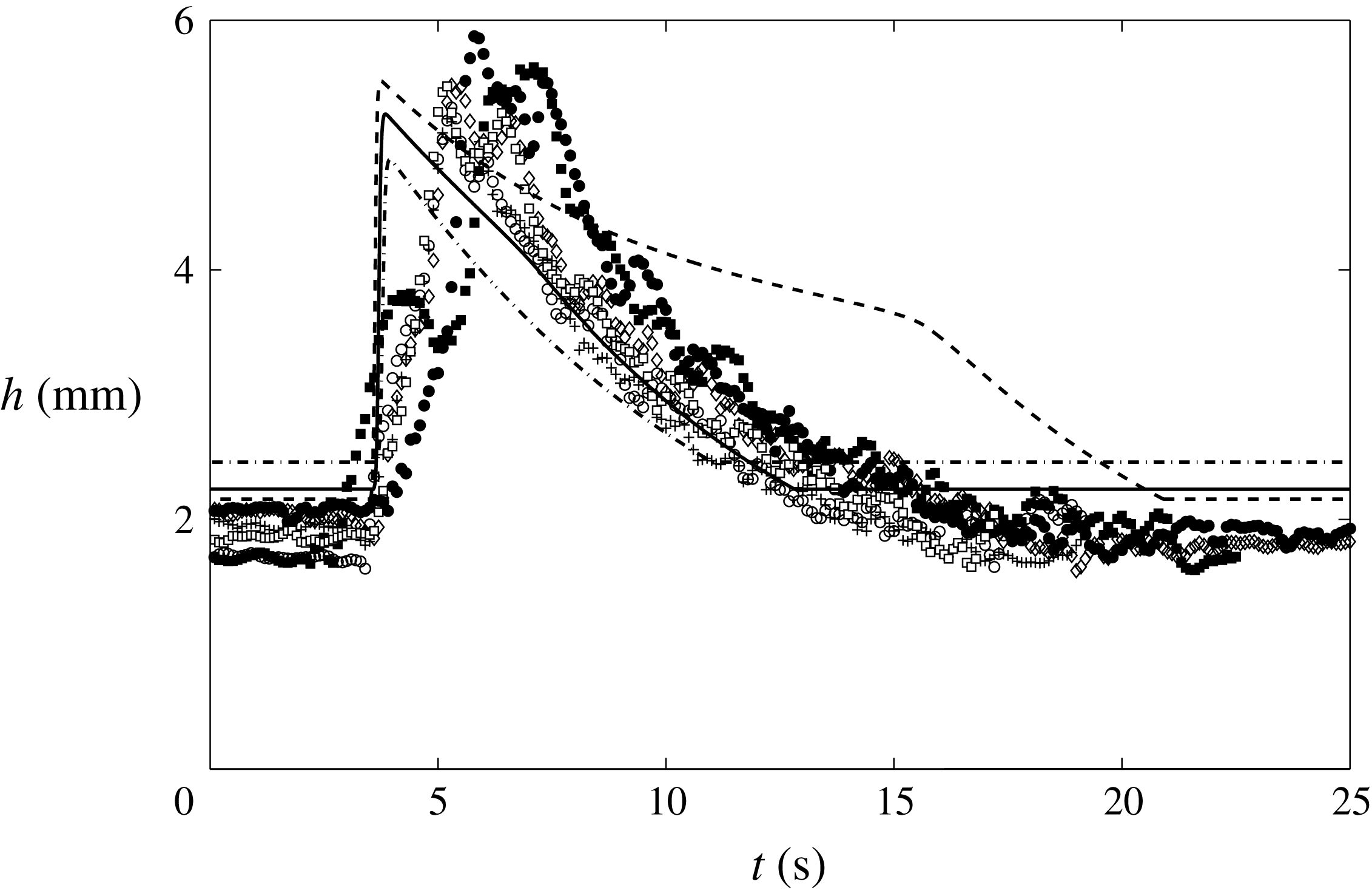
A comparison between all three cases (4.19)–(4.21) and the first six wave crests shown in the space–time plot in figure 3(b) are shown in figure 9. In the experiments the mean wavespeed was found to be
 $u_{w}\approx 0.25\ \text{m}\ \text{s}^{-1}$
and the wavelength was
 ${\it\lambda}\approx 0.59\ \text{m}$
including stationary regions of mean thickness
 $h_{+}\approx 2.0\ \text{mm}$
. Case (4.19) has a wavespeed of
 $u_{w}\approx 0.28\ \text{m}\ \text{s}^{-1}$
and a wavelength excluding stationary regions of
 ${\it\Lambda}\approx 0.49\ \text{m}$
. The solution has a peak thickness of
 $h_{w}\approx 5.5\ \text{mm}$
, giving an amplitude of
 $A\approx 3.3\ \text{mm}$
, which is in good agreement with the experimental values of
 $h_{w}\approx 5.2\ \text{mm}$
and
 $A\approx 3.2\ \text{mm}$
respectively. In terms of these metrics case (4.19) provides the closest fit to the experimental data, which corresponds to the case in which the friction law changes from dynamic to intermediate at a thickness,
 $h_{\star }$
, that is only slightly greater than the minimum value,
 $h_{stop}\approx 3.5358\ \text{mm}$
. There is, however, a marked hump on the lee side of the wave that does not match the observed exponentially decaying tail. A better fit in terms of the shape is provided by case (4.20), although the front is a little too steep and its overall wavelength is too short. In this paper the friction law proposed by Pouliquen & Forterre (Reference Pouliquen and Forterre2002) has been used throughout. It should be noted, however, that in order to modify the shape of the wave subtle changes to the parametrization (3.14)–(3.16) may be needed in future. In addition, the fact that the wavefronts are too steep may be an indication that the viscosity should be larger when the friction is in the intermediate flow regime.
Comparison between experimentally measured erosion–deposition waves and a space–time plot of the travelling-wave solutions. The first six waves of figure 3(b) have been superimposed onto the same arbitrarily chosen start time of
 $t=0\ \text{s}$
, and the travelling-wave solutions of figures 8(a) (dashed line), 8(c) (solid line) and 8(e) (dash-dotted) have been mapped into the time domain with a scaling
 $t\sim -{\it\xi}/u_{w}$
, according to the transformation (4.1).

It is interesting to contrast the steady-state erosion–deposition waves to the case of granular roll waves computed by Gray & Edwards (Reference Gray and Edwards2014) at a fixed slope angle. At a given Froude number for steady uniform flow,
 $\mathit{Fr}_{0}$
, stable limit cycles can be found for roll waves at a range of wave speeds
 $u_{w}\in [1,u_{c}]$
, where
 $u_{c}<1+1/\mathit{Fr}_{0}$
. The steady uniform Froude number and the wave speed therefore parameterize the different states. For granular erosion–deposition waves the thickness
 $h_{\ast }$
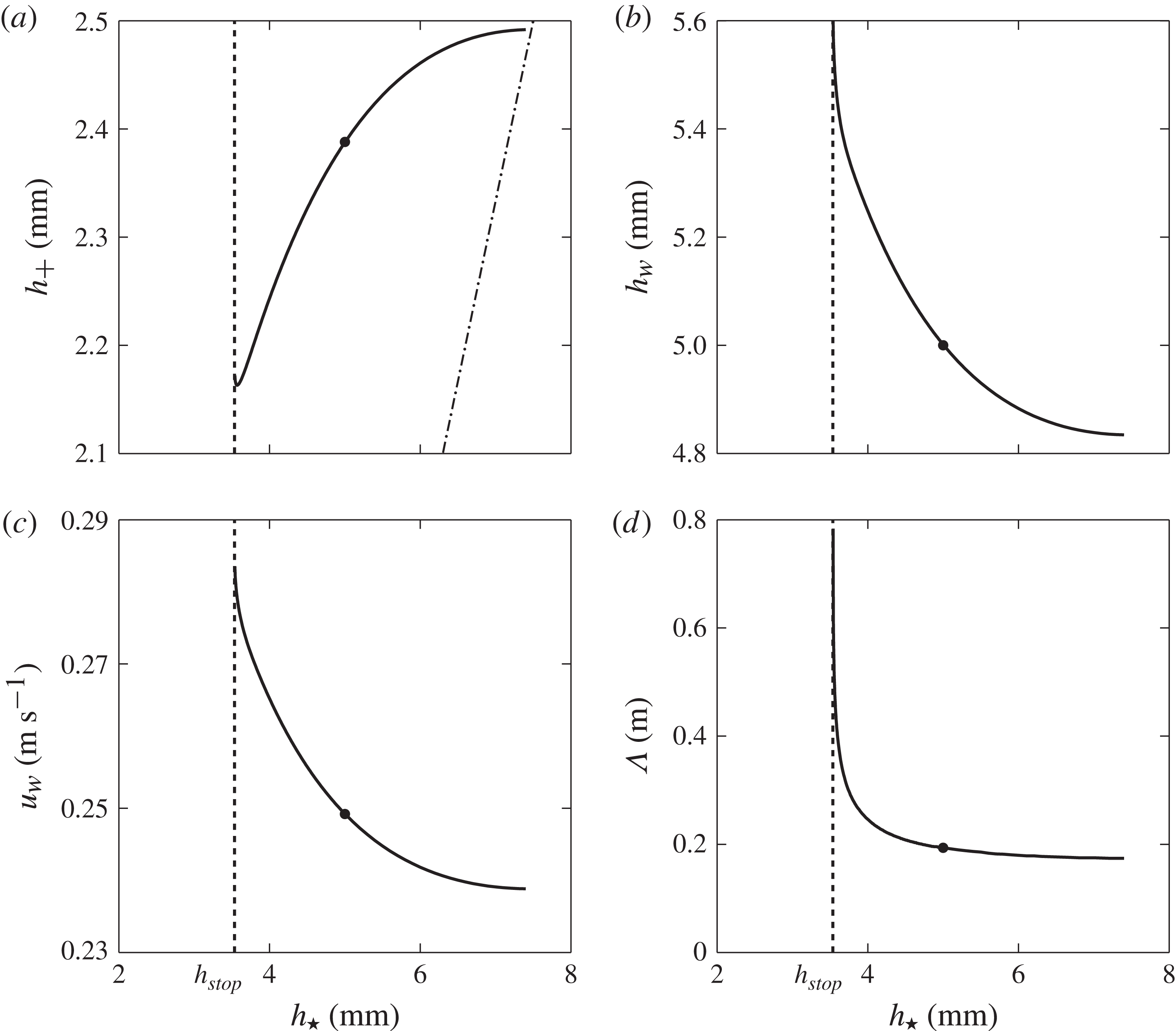
, at which the friction switches from intermediate to dynamic laws, is the only free parameter. Figure 10(a) shows that there is a unique relationship between
 $h_{\ast }$
and the deposit depth
 $h_{+}$
. It follows that erosion–deposition waves are more constrained than roll waves. The graphs in figure 10 show that as
 $h_{\ast }$
increases,
 $h_{+}$
increases, while the peak thickness, wave velocity and wavelength decrease. Large-amplitude erosion–deposition waves therefore travel faster than smaller ones. Solutions whose mobile region lies entirely within the intermediate friction regime lie to the right of the bullet point in each of the subplots. There is also a maximum value for
 $h_{\star }$
, which can be found by differentiating (4.11) with respect to
 $h$
, equating it to zero and substituting
 $h=h_{\star }$
to give
 $$\begin{eqnarray}h_{\star }^{max}=3h_{+}.\end{eqnarray}$$
Admissible values of
 $h_{\star }$
therefore lie in the range
 $[h_{stop},h_{\star }^{max}]$
, which are shown by the dashed and dot-dashed lines in figure 10(a). For all the numerical simulations, presented in §§ 6 and 7, the waves appear to develop into ones of maximum amplitude, with humps, as in figure 8(a), rather than ones with exponentially decaying tails. It is not entirely clear why this is so. It could be that these waves are representative of the most unstable mode, or it could be due to nonlinear coarsening.
Numerical relationship between the input parameters
 $h_{\star }$
and (a)
 $h_{+}$
, for which a valid travelling-wave solution exists to the coupled ODEs (4.15) and (4.16) and the conditions (4.17) and (4.18). Unique solutions exist for
 $h_{\star }\leqslant h_{\star }^{max}=3h_{+}$
(dashed–dotted line). The resulting solutions have (b) peak thickness
 $h_{w}$
, (c) wavespeed
 $u_{w}$
and (d) wavelength
 ${\it\Lambda}$
, exclusive of stationary regions, which varies with
 $h_{\star }$
. Solutions with no transition in the friction law exist for
 $h_{\star }$
greater than the point at which
 $h_{\star }=h_{w}$
(solid markers).

5. Non-existence of solutions without viscous dissipation
The depth-averaged
 ${\it\mu}(I)$
-rheology (Gray & Edwards Reference Gray and Edwards2014) plays a crucial role in modelling erosion–deposition waves. To see this, consider the standard inviscid avalanche model, i.e. (3.1) and (3.2) with
 ${\it\nu}$
equal to zero,
 $$\begin{eqnarray}\displaystyle & \displaystyle {\displaystyle \frac{\partial h}{\partial t}}+{\displaystyle \frac{\partial }{\partial x}}\left(h{\bar{u}}\right)=0, & \displaystyle\end{eqnarray}$$
 $$\begin{eqnarray}\displaystyle & \displaystyle {\displaystyle \frac{\partial }{\partial t}}\left(h{\bar{u}}\right)+{\displaystyle \frac{\partial }{\partial x}}\left(h{\bar{u}}^{2}\right)+{\displaystyle \frac{\partial }{\partial x}}\left(\frac{1}{2}h^{2}g\cos {\it\zeta}\right)=hg\cos {\it\zeta}(\tan {\it\zeta}-{\it\mu}), & \displaystyle\end{eqnarray}$$
 ${\bar{u}}$
has been assumed to be positive everywhere and the shape factor
 ${\it\chi}=1$
. Seeking travelling-wave solutions, the depth-averaged mass balance can be integrated to give the same expression for the depth-averaged velocity as (4.5). Equation (5.2) then reduces to the first-order (rather than second-order) ODE,
 $$\begin{eqnarray}{\displaystyle \frac{\text{d}h}{\text{d}{\it\xi}}}=\frac{(h_{\star }-h_{+})^{2}h^{3}}{(h_{\star }-h_{+})^{2}h^{3}-{\it\beta}^{2}h_{\star }^{3}h_{+}^{2}}\left(\tan {\it\zeta}-{\it\mu}(h)\right),\end{eqnarray}$$
where
 ${\it\mu}(h)$
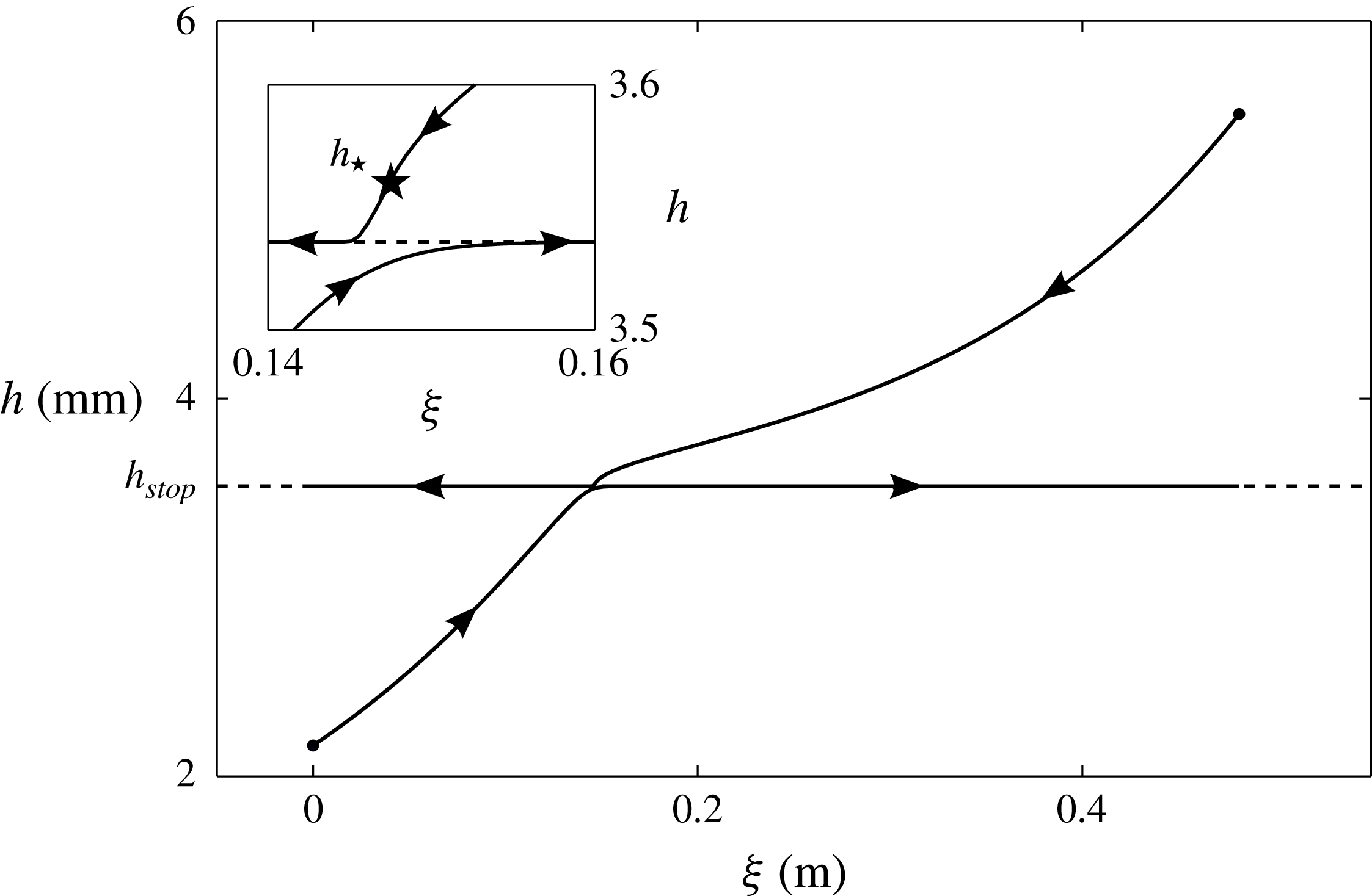
is given in three distinct regions of flow thickness by (4.12)–(4.14). Figure 11 shows numerical solutions of (5.3) for two different initial conditions. Attempting to solve from the rearward side of the wave produces a profile that initially looks very similar to the solution in figure 8(a), but, as the inset in figure 11 shows, it is attracted to a stable fixed point
 $h_{crit}$
that lies very slightly above
 $h_{stop}$
. Conversely, integrating back from the wave peak produces another solution that is initially similar to figure 8(a), but is once again attracted to the fixed point
 $h_{crit}$
. Hence, the two solution branches cannot be connected with the inviscid model.
Travelling-wave solutions to the non-diffusive ODE (5.3), for values of the parameters in (4.19), with initial conditions (solid markers) at the rearward side of the wave and the wave peak. Trajectories are attracted towards a stable fixed point at
 $h=h_{crit}$
, where
 $h_{stop}<h_{crit}\ll h_{\star }$
. In this example
 $h_{crit}$
is only very slightly greater than
 $h_{stop}$
.

The fixed point of the ODE (5.3) occurs when
 $$\begin{eqnarray}M(h)=\tan {\it\zeta}-{\it\mu}(h)=0.\end{eqnarray}$$
Assuming that the friction
 ${\it\mu}(h)$
is given by the intermediate case (4.13) an expansion is made about the point
 $h=h_{stop}$
by the introduction of a new variable
 $\tilde{h}>0$
, where
 $$\begin{eqnarray}h=h_{stop}(1+{\it\kappa}\tilde{h}+O({\it\kappa}^{2}))\end{eqnarray}$$
and
 ${\it\kappa}=10^{-3}$
is the power of extrapolation between the dynamic and static friction law regimes, (4.12) and (4.14), respectively. Substitution of (5.5) into (4.13) and linearizing approximately
 ${\it\kappa}=0$
gives the
 $\tilde{h}$
expansion of (5.4) as
 $$\begin{eqnarray}M(h)={\it\kappa}\left[({\it\mu}_{3}-{\it\mu}_{1})\ln \left(\frac{h_{\star }^{3/2}(h_{stop}-h_{+})}{h_{stop}^{3/2}(h_{\star }-h_{+})}\right)+\frac{{\it\gamma}({\it\mu}_{2}-{\it\mu}_{1})}{(1+{\it\gamma})^{2}}\tilde{h}\right]+O({\it\kappa}^{2}),\end{eqnarray}$$
where the order-unity terms equate to zero by (4.7) and (4.8). It follows that, to leading order,
 $M$
is equal to zero when
 $$\begin{eqnarray}\tilde{h}=\frac{(1+{\it\gamma})^{2}({\it\mu}_{3}-{\it\mu}_{1})}{{\it\gamma}({\it\mu}_{2}-{\it\mu}_{1})}\ln \left(\frac{h_{stop}^{3/2}(h_{\star }-h_{+})}{h_{\star }^{3/2}(h_{stop}-h_{+})}\right)=\tilde{h}_{crit}.\end{eqnarray}$$
The quantity
 $\tilde{h}_{crit}$
is positive, since
 ${\it\gamma}$
is positive (for the range of angles considered here),
 ${\it\mu}_{1}<{\it\mu}_{3}<{\it\mu}_{2}$
and (4.11) implies that the argument in the logarithm is equal to
 ${\it\beta}/\mathit{Fr}(h_{stop})$
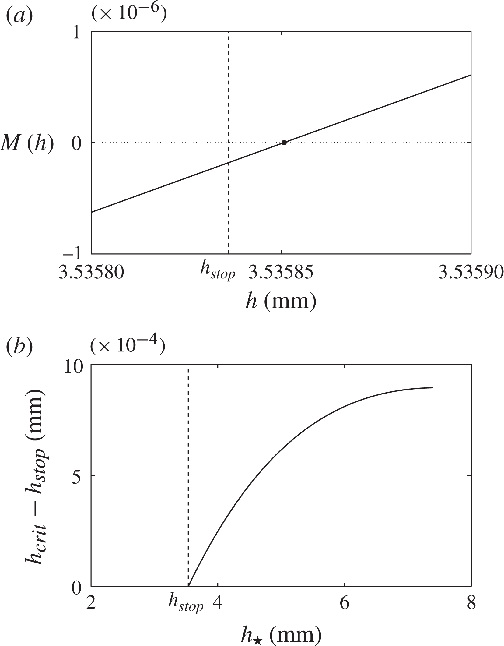
, which is greater than unity. Figure 12(a) shows a plot of
 $M$
as a function of
 $h$
for the parameters
 $h_{\star }$
and
 $h_{+}$
given in (4.19). The approximate solution
 $h_{crit}=h_{stop}(1+{\it\kappa}\tilde{h}_{crit})\approx 3.53585$
(solid marker) is less than
 $h_{\star }=3.56$
. This implies that there is a fixed point in the range
 $[h_{+},h_{\star }]$
, so the inviscid system (5.1) and (5.2) is unable to model the same case as the erosion–deposition wave illustrated in figure 8(a) (where
 $h_{w}>h_{\star }$
). Figure 12(b) shows that
 $h_{stop}\leqslant h_{crit}\ll h_{\star }$
for the complete range of
 $h_{\star }$
. Inviscid solutions starting from the rearward side of the wave will therefore always reach a fixed point, where
 $\text{d}h/\text{d}{\it\xi}=0$
, before the friction law transitions from the intermediate case (4.13) to the dynamic case (4.12). The depth-averaged
 ${\it\mu}(I)$
-rheology is therefore vital to produce the travelling-wave solutions (with
 $h_{w}>h_{\star }$
) that resemble the erosion–deposition waves observed experimentally in § 2.
(a) The value of
 $M$
(solid line) as a function of
 $h$
for parameter values
 $h_{\star }=3.56\ \text{mm}$
and
 $h_{+}\approx 2.16\ \text{mm}$
assumed in the solution (4.19) shown in figure 8(a,b). There is a fixed point when
 $M(h_{crit})=0$
(dotted line) where the ODE (5.3) has zero gradient. An approximate value of
 $h_{crit}$
(solid marker) is found by linearizing the intermediate friction law (4.13) for small
 ${\it\kappa}$
. (b) The approximate value of
 $h_{crit}-h_{stop}$
is given as a function of
 $h_{\star }$
to show that
 $h_{stop}\leqslant h_{crit}<h_{\star }$
for all valid travelling-wave solutions shown in figure 10(a).

6. Numerical method and periodic box simulations
The standard depth-averaged avalanche equations (e.g. Gray et al.
Reference Gray, Tai and Noelle2003) represent a system of hyperbolic equations that require high-resolution shock capturing numerical methods (e.g. Nessyahu & Tadmor Reference Nessyahu and Tadmor1990) to solve them. Although our problems are still convection dominated, the inclusion of the depth-averaged
 ${\it\mu}(I)$
-rheology (Gray & Edwards Reference Gray and Edwards2014) changes the system into a set of convection–diffusion equations. This paper therefore uses the closely related semi-discrete high-resolution non-oscillatory central schemes of Kurganov & Tadmor (Reference Kurganov and Tadmor2000), which use high-order large-step-size ODE solvers for their time evolution. In order to solve the system, the depth-averaged equations (3.1) and (3.2) together with the friction law (3.14)–(3.16) are written in vector form as
 $$\begin{eqnarray}{\displaystyle \frac{\partial \boldsymbol{w}}{\partial t}}+{\displaystyle \frac{\partial \boldsymbol{f}(\boldsymbol{w})}{\partial x}}=\boldsymbol{S}(\boldsymbol{w})+{\displaystyle \frac{\partial }{\partial x}}\left(\boldsymbol{Q}(\boldsymbol{w},\boldsymbol{w}_{x})\right),\end{eqnarray}$$
where
 $\boldsymbol{w}=(h,m)^{\text{T}}$
is the vector of conserved variables,
 $h$
and
 $m=h{\bar{u}}$
. The resulting convection flux
 $\boldsymbol{f}$
and source term
 $\boldsymbol{S}$
are
 $$\begin{eqnarray}\boldsymbol{f}=\left(\begin{array}{@{}c@{}}m\\ {\displaystyle \frac{m^{2}}{h}}+{\displaystyle \frac{h^{2}}{2}}g\cos {\it\zeta}\end{array}\right),\quad \boldsymbol{S}=\left(\begin{array}{@{}c@{}}0\\ hg\left(\sin {\it\zeta}-{\it\mu}{\displaystyle \frac{m}{|m|}}\cos {\it\zeta}\right)\end{array}\right),\end{eqnarray}$$
respectively, and the diffusive flux
 $\boldsymbol{Q}$
is
 $$\begin{eqnarray}\boldsymbol{Q}=\left(\begin{array}{@{}c@{}}0\\ {\it\nu}h^{1/2}\left({\displaystyle \frac{\partial m}{\partial x}}-{\displaystyle \frac{m}{h}}{\displaystyle \frac{\partial h}{\partial x}}\right)\end{array}\right).\end{eqnarray}$$
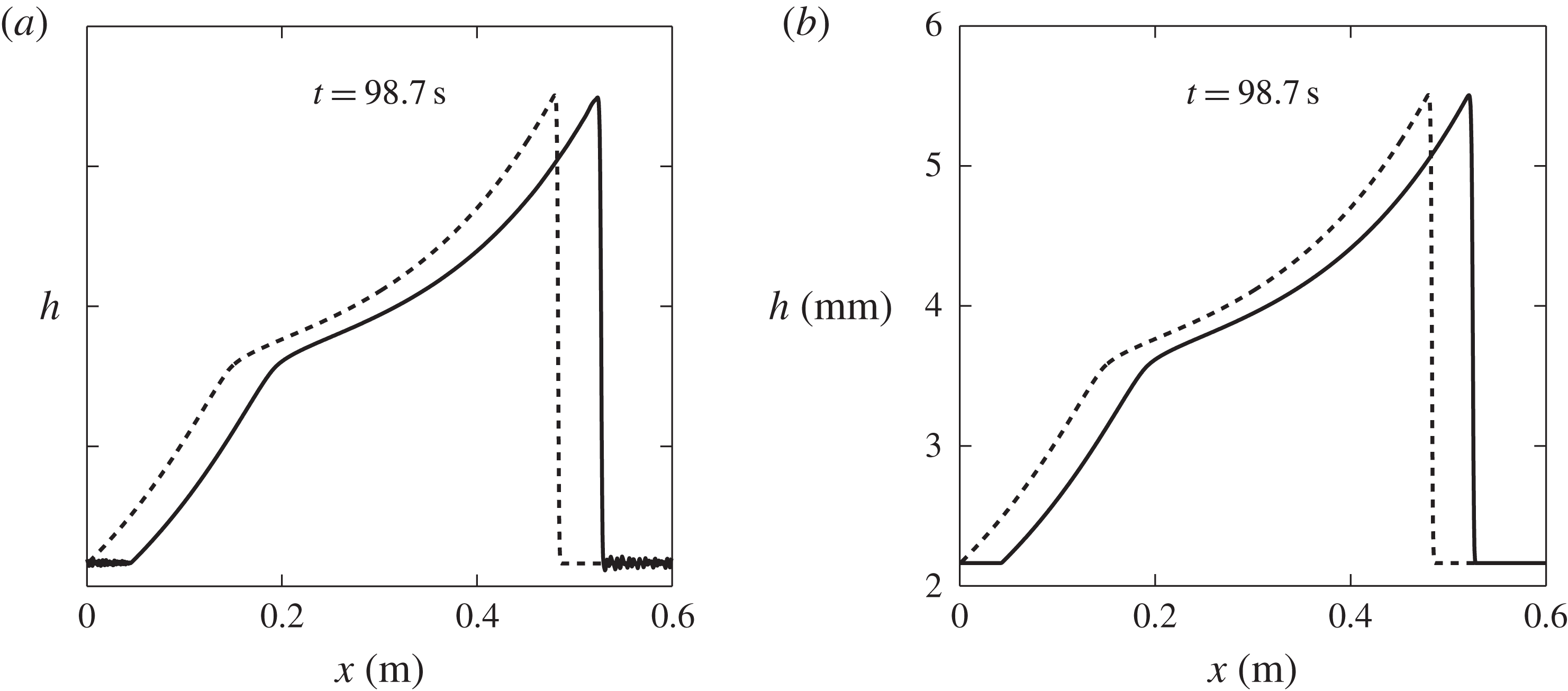
Periodic box simulations are performed using the travelling-wave solution illustrated in figure 8(a) as an initial condition. This is determined by the parameters summarized in table 1, together with
 $h_{+}$
and
 $h_{\star }$
given in (4.19) and the depth-averaged velocity computed from (4.5) and (4.10). The domain length
 $L$
is set to 0.6 m and is discretized over 1200 grid points. The travelling wave is allowed to evolve on the periodic domain and the resulting flow thickness is shown at
 $t=98.7\ \text{s}$
in figure 13 for (a) a second-order Runge–Kutta method with a step size of
 $10^{-2}\ \text{s}$
and (b) a third-order Runge–Kutta adaptive step method (Medovikov Reference Medovikov1998). Both methods preserve the initial form of the wave (shown as a dashed line) over the mobile section, but the second-order Runge–Kutta method encounters some problems in properly handling the stationary region. The standard deviation of the static layer from its mean value is
 $1.73\times 10^{-5}\ \text{mm}$
, which is significantly larger than
 $4.26\times 10^{-9}\ \text{mm}$
for the third-order Runge–Kutta scheme. However, simulation times with the third-order method are much longer than with the second-order Runge–Kutta time-stepper, particularly when stationary regions of flow develop, since the adaptive step size reduces drastically. As such, it is impractical to adopt this time-stepper for all of the numerical results and the second-order Runge–Kutta time-stepper is used hereafter. Numerical simulations have also been performed for waves that do not transition to the dynamic flow regime, such as those illustrated in figure 8(e). For simulations on a box of length 0.3 m the solution is stable, but on the 0.6 m box the solution transforms into one that resembles the solution in figure 8(c), where
 $h_{\star }<h_{w}$
. This may be an indication that such waves, whose mobile section lies purely in the intermediate friction regime, are physically unstable.
Flow thickness
 $h$
varying with downslope position
 $x$
(solid lines), obtained from numerical simulations on a periodic domain with the travelling-wave solution from figure 8(a) as the initial condition (dashed lines). The flow thickness profile is observed to remain unchanged, apart from small variations in the constant thickness
 $h_{+}$
of the stationary layer. These variations are greater with the second-order Runge–Kutta time-stepper (a) than with the third-order adaptive Runge–Kutta time-stepper (b). Two movies showing the time-dependent evolution of the waves are available in the online supplementary material.

6.1. Random perturbation about steady uniform flow
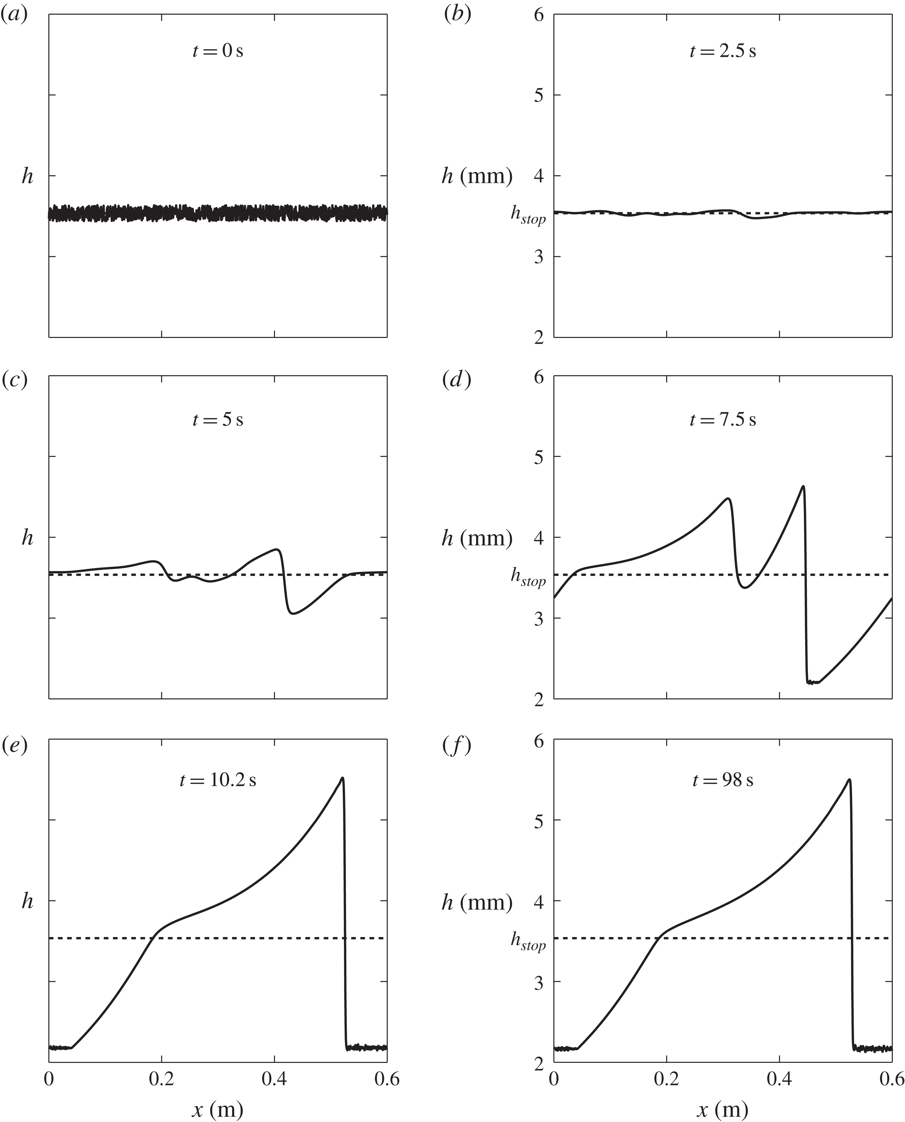
For the same periodic domain and grid resolution the evolution of an erosion–deposition wave in time is computed for an initially steady uniform flow of thickness
 $h_{0}$
and velocity
 $$\begin{eqnarray}{\bar{u}}_{0}=\frac{{\it\beta}\sqrt{g\cos {\it\zeta}}}{\mathscr{L}{\it\gamma}}h_{0}^{3/2}.\end{eqnarray}$$
To trigger the instability, a pseudo-random perturbation,
 $R(x)$
, which takes a different value in the interval
 $[-1,1]$
at each grid point, is added to the initial condition, i.e.
 $$\begin{eqnarray}h(x,0)=h_{0}+{\it\varepsilon}R(x),\quad m(x,0)=m_{0}=h_{0}{\bar{u}}_{0},\end{eqnarray}$$
where
 ${\it\varepsilon}=10^{-4}$
is the magnitude of the zero-mean perturbation. Figure 14 shows a typical numerical simulation of the evolving flow thickness for the case
 $$\begin{eqnarray}h_{0}=h_{stop}=\mathscr{L}{\it\gamma},\quad {\bar{u}}_{0}={\bar{u}}_{stop}={\it\beta}\sqrt{\mathscr{L}g\cos {\it\zeta}}.\end{eqnarray}$$
The surface becomes unstable and small waves form which interact and grow in size before reaching a final state in figure 14(e), which survives indefinitely as shown at a much later time ( f). The wavespeed of the erosion–deposition wave is
 $u_{w}=0.28\ \text{m}\ \text{s}^{-1}$
and the peak height and stationary layer thickness are found to be
 $h_{w}=5.5\ \text{mm}$
and
 $h_{+}=2.2\ \text{mm}$
respectively, resulting in an amplitude of
 $A=3.3\ \text{mm}$
. These closely match those of the travelling-wave solution in figure 8(a), which provides further validation of the method.
The flow thickness
 $h$
obtained by a numerical simulation in a periodic domain with initial conditions
 $h(x,0)=h_{stop}+10^{-4}R(x)$
, where
 $R(x)\in [-1,1]$
is a zero-mean pseudo-random perturbation to the thickness
 $h_{stop}$
of a steady uniform flow. The perturbations grow in size and eventually coarsen to form a single erosion–deposition wave. The solution is plotted at various times, with the final state, first reached in (e), surviving forever ( f). A movie showing the time-dependent evolution is available in the online supplementary material.

Results of a numerical simulation at time
 $t=23.5\ \text{s}$
showing (a) the flow thickness
 $h$
and (b) the depth-averaged velocity
 ${\bar{u}}$
with downslope position
 $x$
(solid lines). At the inflow boundary the flow thickness
 $h(0,t)=h_{stop}+10^{-4}\sin (2{\rm\pi}ft)$
is prescribed, where the sinusoidal perturbation has frequency
 $f=0.47\ \text{Hz}$
. Initially, there is a steady uniform flow with
 $h_{0}=h_{stop}$
and
 ${\bar{u}}_{0}={\bar{u}}_{stop}$
(dashed lines). The important experimental flow feature of stationary regions between waves, where
 ${\bar{u}}=0$
, is captured numerically. A movie showing the time-dependent evolution is available in the online supplementary material.

7. Numerical simulations of erosion–deposition waves in a chute
To compare the model with the experimental results of § 2, one-dimensional numerical simulations are performed for a chute geometry. Initially, a steady uniform flow is assumed along the complete length of the chute,
 $$\begin{eqnarray}h(x,0)=h_{0},\quad m(x,0)=m_{0}=h_{0}{\bar{u}}_{0},\quad \forall x\in [0,L],\end{eqnarray}$$
where
 $h_{0}\geqslant h_{stop}$
. The boundary conditions at the start and end of the chute are still dominated by the those of the convective problem, since inclusion of the depth-averaged
 ${\it\mu}(I)$
-rheology is a singular perturbation to the equations. For the problems of interest here the flows are subcritical (
 $\mathit{Fr}<1$
) everywhere, which requires one upstream and one downstream condition to be specified for the hyperbolic system (e.g Weiyan Reference Weiyan1992). The introduction of a diffusive term means that the system is now parabolic and an extra boundary condition is required, which is applied here at the outflow end (
 $x=L$
), where free outflow is imposed via linear extrapolations of the values of
 $h$
and
 $m$
from the final two interior cells. At the upstream boundary,
 $x=0$
, the general inflow condition is
 $$\begin{eqnarray}h(0,t)=h_{0}+{\it\varepsilon}H(t),\end{eqnarray}$$
where
 ${\it\varepsilon}=10^{-4}$
is the magnitude of the perturbation,
 $H(t)$
. For the simulations performed here, erosion–deposition waves develop in the range
 $h_{0}\in [h_{stop},1.025h_{stop}]$
. The flow stops for
 $h_{0}<h_{stop}$
, and for
 $h_{0}>1.025h_{stop}$
granular roll waves form, which are fully mobilized and do not have stopping regions.
7.1. Sinusoidal inflow perturbation
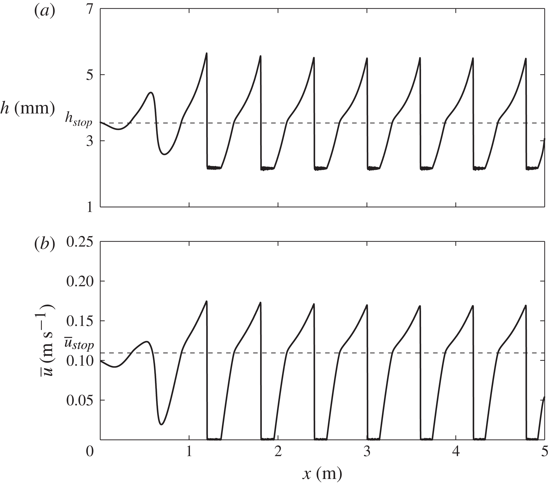
A series of travelling erosion–deposition waves can be generated by imposing a small sinusoidal perturbation to a steady uniform flow of thickness
 $h_{stop}$
, i.e.
 $$\begin{eqnarray}h_{0}=h_{stop},\quad H(t)=\sin (2{\rm\pi}ft),\end{eqnarray}$$
where the oscillation frequency is set to
 $f=0.47\ \text{Hz}$
. The computed flow thickness
 $h$
and depth-averaged velocity
 ${\bar{u}}$
are shown in figure 15 for a domain length of
 $L=5\ \text{m}$
using 10 000 grid points. The perturbations rapidly grow into erosion–deposition waves that closely resemble the travelling wave shown in figure 8(a). The distance between successive wavefronts is
 ${\it\lambda}\approx 0.60\ \text{m}$
(including the stationary regions), and wavefronts pass a given point at regular intervals with a period
 $T\approx 2.13\ \text{s}$
, implying a wavespeed of
 $u_{w}\approx 0.28\ \text{m}\ \text{s}^{-1}$
. This is consistent with the imposed perturbation. The resulting peak thickness,
 $h_{w}\approx 5.5\ \text{mm}$
, layer thickness,
 $h_{+}\approx 2.2\ \text{mm}$
, and wave amplitude,
 $A=3.3\ \text{mm}$
, are all in good quantitative agreement with the experimentally obtained values. However, since all the waves have the same height and wavespeed they do not produce wave merging events like those observed in figure 3(a).
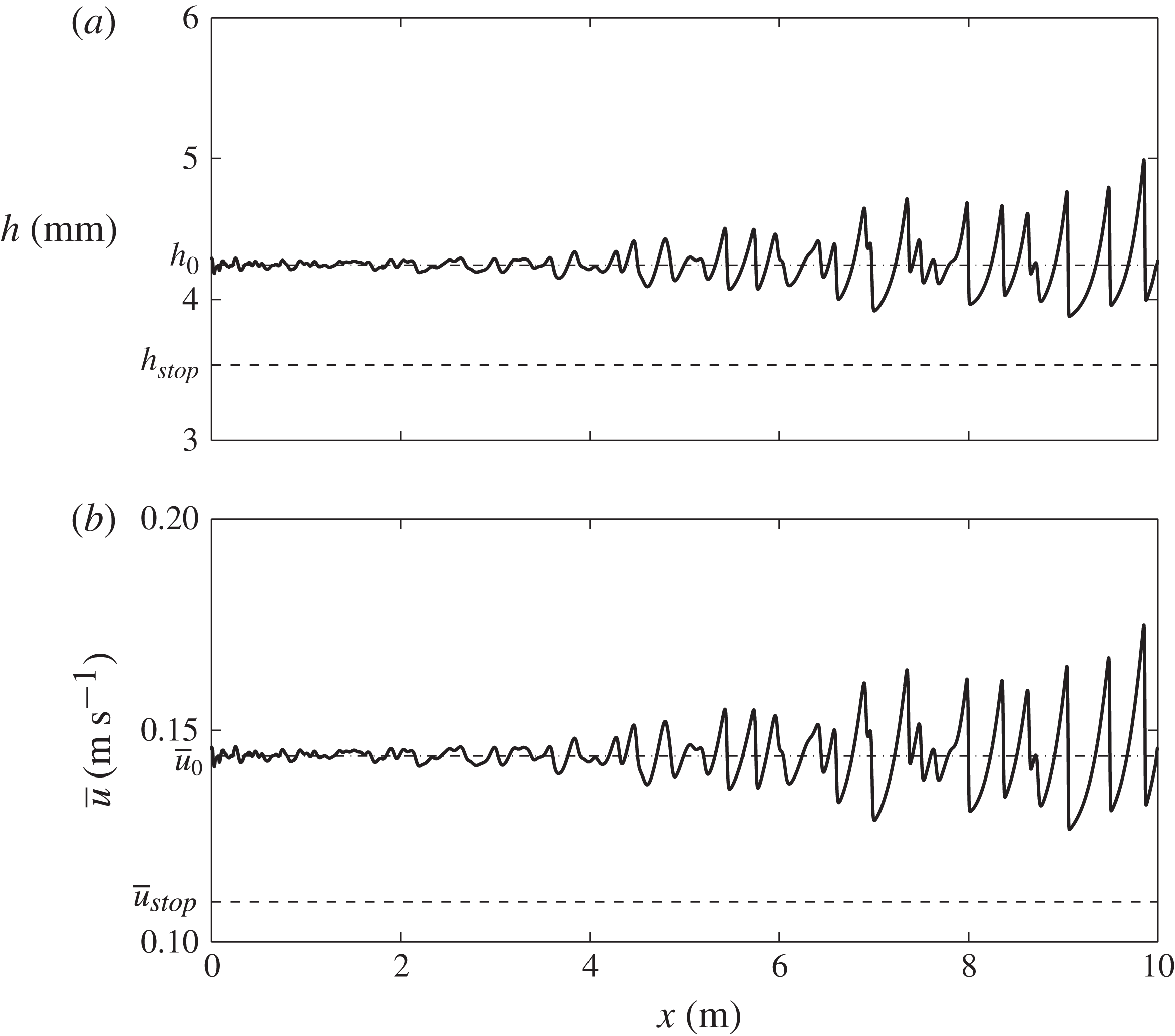
Results of a numerical simulation at time
 $t=23.5\ \text{s}$
showing (a) the flow thickness
 $h$
and (b) the depth-averaged velocity
 ${\bar{u}}$
with downslope position
 $x$
(solid lines). At the inflow boundary, a flow thickness
 $h(0,t)=h_{stop}+10^{-4}R(t)$
is prescribed, where
 $R(t)\in [-1,1]$
is a zero-mean pseudo-random perturbation. A steady uniform flow of thickness
 $h_{stop}$
and corresponding depth-averaged velocity
 ${\bar{u}}_{stop}$
is imposed as an initial condition (dashed lines). A movie showing the time-dependent evolution is available in the online supplementary material.

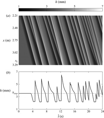
Results of a numerical simulation for an inflow thickness
 $h(0,t)=h_{stop}+10^{-4}R(t)$
, where
 $R(t)\in [-1,1]$
is a zero-mean pseudo-random perturbation. Steady uniform flow of thickness
 $h_{stop}$
and depth-averaged velocity
 ${\bar{u}}_{stop}$
is imposed as an initial condition. Data are given between times
 $\hat{t}$
of 0 and 24 s for (a) a space–time plot (with flow thickness given by the greyscale colourbar) of the downslope region
 $2.21\ \text{m}\leqslant x\leqslant 3.29\ \text{m}$
and (b) the flow thickness past the point
 $x_{L}=3.21\ \text{m}$
, corresponding with the experimental results in figure 3. The important experimental flow features of stationary regions between waves of a constant wavespeed (straight diagonal lines) and merging events (where lines representing waves of a different speed meet) are all captured numerically.

7.2. Random inflow perturbation
In order to produce merging, the form of the perturbation,
 $H(t)$
, is now chosen to be a pseudo-random zero-mean function
 $R(t)$
, which takes a value in the interval
 $[-1,1]$
at each time step, i.e. the inflow conditions are
 $$\begin{eqnarray}h_{0}=h_{stop},\quad H(t)=R(t).\end{eqnarray}$$
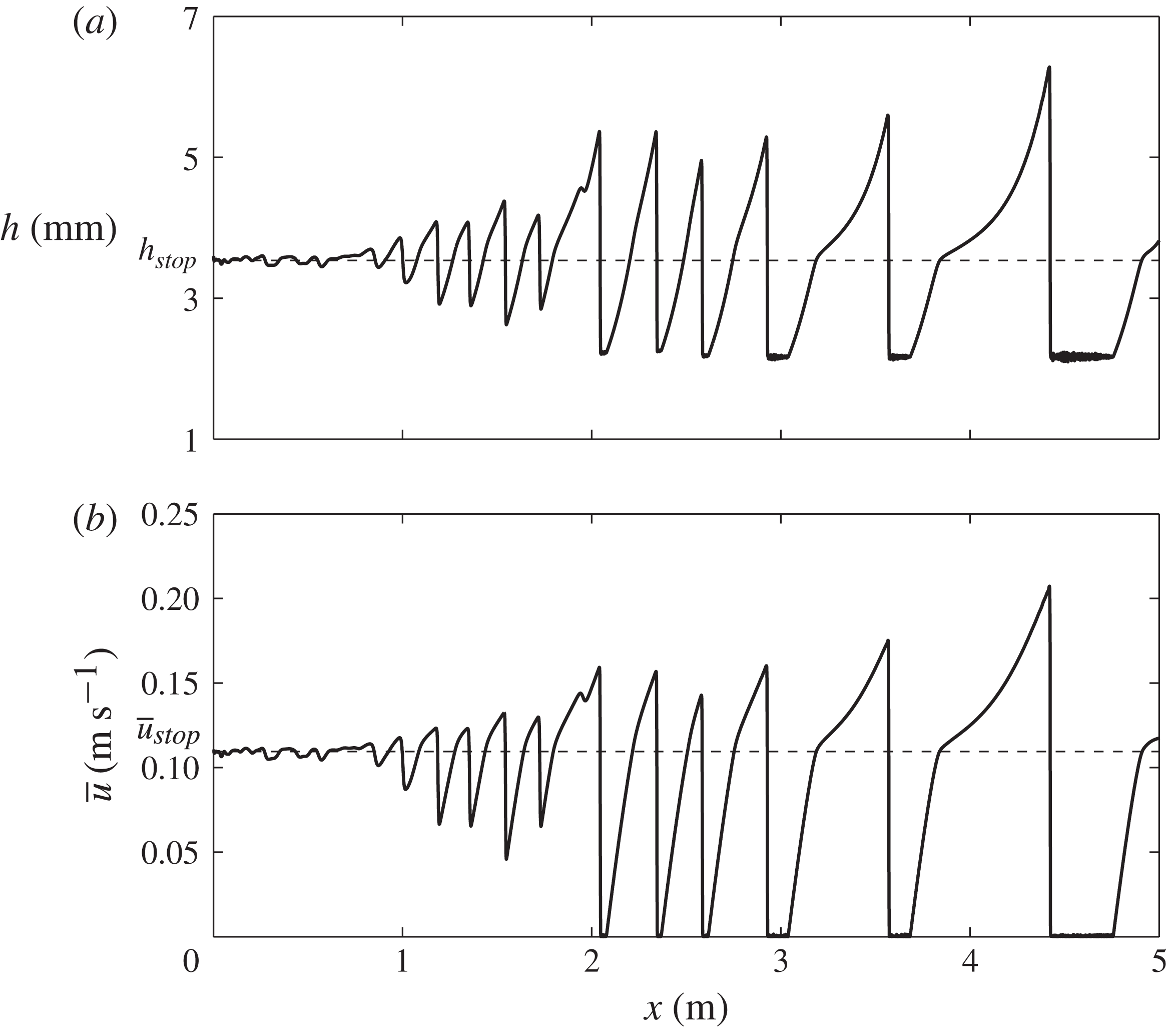
The spatial evolutions of the computed flow thickness
 $h$
and the depth-averaged velocity
 ${\bar{u}}$
are shown in figure 16 at a fixed time. A corresponding video of the simulation is also available in the online supplementary material. The random inflow condition generates erosion–deposition waves with different characteristic frequencies and wavespeeds, which merge with one another. This delays the formation of stationary regions, which only start to develop between two and three metres downstream, as compared with the sinusoidal case, where they form just after the first metre. The merging events can be visualized by generating a space–time plot for the region between
 $x=2.20$
and 3.29 m, as shown in figure 17(a), which shows diagonal wavefront lines meeting in a similar way to the experiment shown in figure 3(a). Since the data acquisition was started at an arbitrary time, the simulation time
 $\hat{t}$
is shifted, i.e.
 $\hat{t}=t-7.5\ \text{s}$
, in order to compare directly with the experimental data. The wavespeed of each erosion–deposition wave is determined by the gradient of the corresponding diagonal line in the space–time plot (figure 17
a) and is found here to have a value of
 $u_{w}\approx 0.27\ \text{m}\ \text{s}^{-1}$
. The period between successive wavefronts, inclusive of stationary regions (given by the horizontal length of time between the wavefronts), is found to have a mean value of
 $T\approx 2.13\ \text{s}$
and a corresponding mean frequency of
 $f\approx 0.47\ \text{Hz}$
. Combination of these gives the mean wavelength of each roll wave, including a stationary region, as
 ${\it\lambda}\approx 0.58\ \text{m}$
. Figure 17(b) shows the flow thickness past the point
 $x_{L}=3.21\ \text{m}$
downslope as a function of time. It indicates that the mean peak thickness is
 $h_{w}\approx 5.4\ \text{mm}$
and the mean stationary layer depth is
 $h_{+}\approx 2.2\ \text{mm}$
, implying a wave amplitude of approximately 3.2 mm. These are all in good qualitative agreement with the experimentally obtained values. The Pouliquen–Forterre friction law (Pouliquen & Forterre Reference Pouliquen and Forterre2002), together with the depth-averaged
 ${\it\mu}(I)$
-rheology (Gray & Edwards Reference Gray and Edwards2014), is therefore able to quantitatively model the formation of erosion–deposition waves with stationary regions.
8. Contrast to numerical simulations of granular roll waves
Using exactly the same depth-averaged equations (3.1) and (3.2) together with the friction law (3.14)–(3.16) it is also possible to simulate the formation of granular roll waves, such as those observed in experiments (e.g. Davies Reference Davies1990; Vallance Reference Vallance1994; Forterre & Pouliquen Reference Forterre and Pouliquen2003; Zanuttigh & Lamberti Reference Zanuttigh and Lamberti2007; Iverson et al.
Reference Iverson, Logan, LaHusen and Berti2010; Gray & Edwards Reference Gray and Edwards2014). Roll waves develop in thicker flows (
 $h_{0}>h_{stop}$
) in which the Froude number,
 $\mathit{Fr}$
, remains greater than
 ${\it\beta}$
throughout. This implies that the friction coefficient is always in the dynamic regime (3.14), although this is not enforced in the simulations. Initially, the chute is therefore assumed to contain a steady uniform flow, as in (7.1), that is slightly deeper
 $$\begin{eqnarray}h_{0}=1.2h_{stop},\quad m_{0}=h_{0}{\bar{u}}_{0}=(1.2)^{5/2}h_{stop}{\bar{u}}_{stop},\end{eqnarray}$$
where
 ${\bar{u}}_{0}=(1.2)^{3/2}{\bar{u}}_{stop}$
follows from (6.4) and (6.6). Since roll waves take longer to form than erosion–deposition waves, the domain length is doubled to
 $L=10\ \text{m}$
and is discretized over 20 000 grid points, to match the resolution of the previous simulations.
8.1. Sinusoidal inflow perturbation
Since the inflow condition is still subcritical (
 $\mathit{Fr}<1$
), only the upstream flow height and its sinusoidal perturbation need to be prescribed at
 $x=0$
, i.e.
 $$\begin{eqnarray}h_{0}=1.2h_{stop},\quad H(t)=\sin (2{\rm\pi}ft),\end{eqnarray}$$
where the perturbation frequency
 $f=0.47\ \text{Hz}$
is the same as in (7.3). The computed flow thickness,
 $h$
, and the depth-averaged velocity,
 ${\bar{u}}$
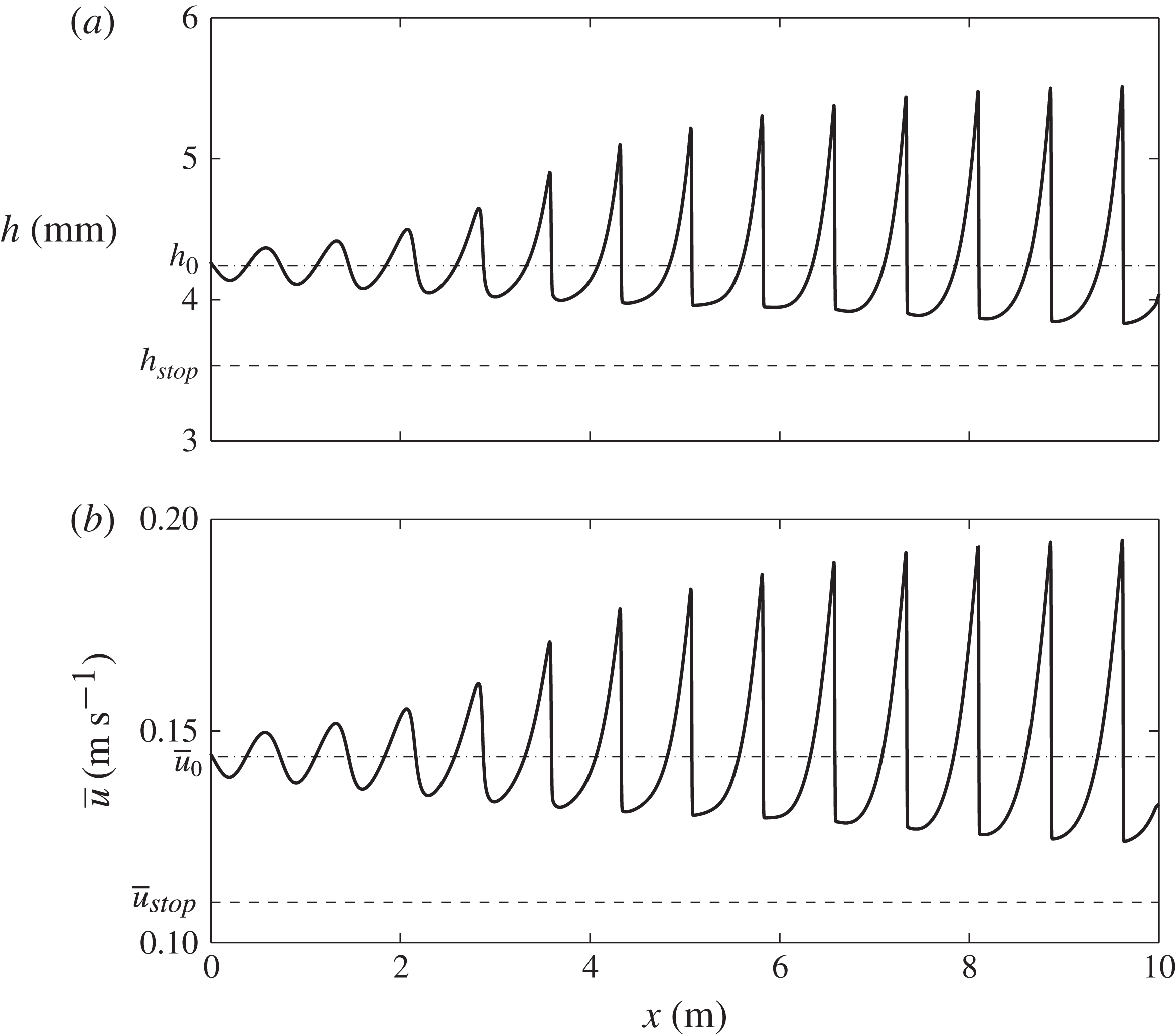
, are shown in figure 18. Since the uniform flow is unstable to the small perturbations at the inflow, these grow into fully developed granular roll waves of the imposed frequency by approximately 8 m downstream. This is significantly further than the sinusoidally induced erosion–deposition waves which were fully developed after approximately 1 m. During the evolution none of the troughs between the wave crests lie below
 $h_{stop}$
and so no stationary regions form. On examining the flow thickness at the outflow end of the domain, when a steady state has been reached, it can be seen that although each wave has a peak thickness of
 $h_{w}\approx 5.5\ \text{mm}$
, similar to the erosion–deposition wave case, the troughs have a much greater thickness,
 $h_{trough}\approx 3.8\ \text{mm}$
. This implies that continuous waves, despite developing from a greater inflow thickness than their erosion–deposition wave counterparts, have a much smaller wave amplitude of
 $A\approx 1.7\ \text{mm}$
, for an inflow perturbation oscillating with the same amplitude and frequency.
Results of a numerical simulation at time
 $t=40.0\ \text{s}$
showing (a) the flow thickness
 $h$
and (b) the depth-averaged velocity
 ${\bar{u}}$
with downslope position
 $x$
(solid lines). At the inflow boundary a flow thickness
 $h(0,t)=1.2h_{stop}+10^{-4}\sin (2{\rm\pi}ft)$
with sinusoidal perturbation frequency
 $f=0.47\ \text{Hz}$
is imposed. The initial steady uniform flow thickness
 $h_{0}=1.2h_{stop}$
and depth-averaged velocity
 ${\bar{u}}_{0}=(1.2)^{3/2}{\bar{u}}_{stop}$
are shown by the dot-dashed lines. The minimum flow thickness and velocity,
 $h_{stop}$
and
 ${\bar{u}}_{stop}$
, are shown with dashed lines. A movie showing the time-dependent evolution is available in the online supplementary material.

8.2. Random inflow perturbation
The pseudo-random zero-mean form of the inflow perturbation function, with
 $R(t)\in [-1,1]$
at each time step, is now applied, i.e.
 $$\begin{eqnarray}h_{0}=1.2h_{stop},\quad H(t)=R(t).\end{eqnarray}$$
The flow thickness
 $h$
and depth-averaged velocity
 ${\bar{u}}$
are shown in figure 19 for one fixed time,
 $t$
, of a typical random simulation. A corresponding video of the simulation is also available in the online supplementary material in order to compare and contrast it to the formation of erosion–deposition waves. Continuous roll waves of a range of characteristic frequencies and wavespeeds develop downstream of the inflow. On examining the flow thickness at the outflow end of this domain, the wave peaks have a mean flow thickness of
 $h_{w}\approx 4.8\ \text{mm}$
, whilst the troughs have a mean thickness of
 $h_{trough}\approx 3.9\ \text{mm}$
. This implies a mean wave amplitude of only
 $A=0.9\ \text{mm}$
, despite many merging events and wave coarsening having taken place on a domain that is twice the length. This is consistent with the experimental observations of Forterre & Pouliquen (Reference Forterre and Pouliquen2003), who had to use a loudspeaker system to induce moderately large perturbations with a given frequency in order to see roll waves on their 2 m long chute. The granular roll waves look qualitatively different in shape to erosion–deposition waves and their coarsening dynamics also appears to be very different. The most notable difference, however, is that erosion–deposition waves have stationary regions.
Results of a numerical simulation at time
 $t=40.0\ \text{s}$
showing (a) the flow thickness
 $h$
and (b) the depth-averaged velocity
 ${\bar{u}}$
with downslope position
 $x$
(solid lines). At the inflow boundary, a flow thickness
 $h(0,t)=1.2h_{stop}+10^{-4}R(t)$
is prescribed, where
 $R(t)\in [-1,1]$
is a zero-mean pseudo-random perturbation. The initial flow thickness
 $h_{0}=1.2h_{stop}$
and corresponding depth-averaged velocity
 ${\bar{u}}_{0}=(1.2)^{3/2}{\bar{u}}_{stop}$
are shown with dot-dashed lines. The minimum flow thickness and velocity for which a steady uniform flow is possible,
 $h_{stop}$
and
 ${\bar{u}}_{stop}$
, are also shown using dashed lines. A movie showing the time-dependent evolution is available in the online supplementary material.

9. Conclusions
In this paper experiments are used to show that a granular avalanche close to the minimum depth for steady uniform flow,
 $h_{stop}$
, can spontaneously break down into a series of discrete erosion–deposition waves that are separated by regions of completely static grains. We believe that each individual wave is directly related to the isolated triangular waves first reported in the literature by Daerr (Reference Daerr2001). The waves are able to travel downslope at constant speed, steadily eroding and depositing a static erodible layer, ahead of and behind them, in exact balance, so that their shape is preserved. Remarkably, given the notorious difficulty in modelling erosion–deposition problems, a quantitative depth-averaged theory has been developed for these waves by combining the depth-averaged
 ${\it\mu}(I)$
-rheology of Gray & Edwards (Reference Gray and Edwards2014) with the dynamic, intermediate and static friction regimes in Pouliquen & Forterre’s (Reference Pouliquen and Forterre2002) extended friction law. Rather than progressively eroding and/or depositing the grains from the base of the avalanche, this approach treats the regions as either mobile or static throughout their depth. This necessarily imposes a limitation on the model’s applicability, since the depth of the erodible material has to be shallow, i.e. it is not possible to calculate the erosion and deposition on slopes with an arbitrary depth of static grains. However, it is encouraging that a model constructed in this fashion captures much of the observed behaviour.
It is the combination of the viscous dissipation introduced through the
 ${\it\mu}(I)$
-rheology (Gray & Edwards Reference Gray and Edwards2014) and Pouliquen & Forterre’s (Reference Pouliquen and Forterre2002) intermediate friction law (3.15) (for
 $0<\mathit{Fr}<{\it\beta}$
) that is able to bring the grains to rest. Indeed, we have shown in § 5 that it is not possible to construct travelling erosion–deposition waves using a standard inviscid avalanche model (e.g. Savage & Hutter Reference Savage and Hutter1989; Gray et al.
Reference Gray, Wieland and Hutter1999; Pouliquen & Forterre Reference Pouliquen and Forterre2002; Gray et al.
Reference Gray, Tai and Noelle2003). This problem is therefore one of those occasions where the rheology, which is normally negligibly small, plays a crucial role in the solution.
The depth-averaged
 ${\it\mu}(I)$
-rheology changes the standard hyperbolic avalanche model into a system of convection–diffusion equations. A numerical method to solve the full depth-averaged equations (3.1) and (3.2) together with the friction law (3.14)–(3.16) has been developed, which is based on the semi-discrete high-resolution non-oscillatory central schemes of Kurganov & Tadmor (Reference Kurganov and Tadmor2000). This uses efficient high-order large-step-size ODE solvers for their time evolution, which allow the diffusive terms to be included while preserving the advantages of explicit methods for convection-dominated problems. The method is able to compute the formation of erosion–deposition waves from a steady uniform flow of depth
 $h=h_{stop}$
, which is on the boundary of being able to flow. Figure 16 shows results for a very small pseudo-random perturbation to the inflow thickness
 $h_{stop}=3.53\ \text{mm}$
that is able to quantitatively reproduce typical peak flow thicknesses,
 $h_{w}=5.4\ \text{mm}$
, static deposit depths,
 $h_{+}\approx 2.2\ \text{mm}$
, wavespeeds,
 $u_{w}\approx 0.27\ \text{m}\ \text{s}^{-1}$
, and typical wavelengths,
 ${\it\lambda}=0.58\ \text{m}$
, consistent with those observed in the experiments described in § 2. Moreover, a space–time plot in figure 17 shows that variation in individual wave speeds leads to coarsening similar to that observed in experiment (as shown in figure 3).
The theory presented here is also able to model the formation of granular roll waves for
 $h>1.025h_{stop}$
, such as those observed experimentally (e.g. Davies Reference Davies1990; Vallance Reference Vallance1994; Forterre & Pouliquen Reference Forterre and Pouliquen2003; Zanuttigh & Lamberti Reference Zanuttigh and Lamberti2007; Iverson et al.
Reference Iverson, Logan, LaHusen and Berti2010; Gray & Edwards Reference Gray and Edwards2014). Roll waves are in some ways simpler than erosion–deposition waves, because the friction stays entirely within the dynamic regime (
 $\mathit{Fr}>{\it\beta}$
) given by (3.14). The introduction of viscous dissipation allows continuous roll waves to form, with no stopping regions, i.e.
 ${\bar{u}}>0$
everywhere. The amplitudes of granular roll waves are significantly smaller than their erosion–deposition wave counterparts, and they take a much greater distance to fully develop, which is consistent with experiments. As the inflow thickness is decreased, roll waves transition into erosion–deposition waves in a narrow regime just above
 $h_{stop}$
. Inflow thicknesses below
 $h_{stop}$
rapidly come completely to rest. It is interesting, and perhaps very significant, that flows on the very cusp of stopping spontaneously self-organize to produce large-amplitude waves that sustain the flow.
Acknowledgements
This research was supported by NERC grants NE/E003206/1 and NE/K003011/1 as well as EPSRC grants EP/I019189/1 and EP/K00428X/1. N.G. acknowledges support from the program on ‘Fluid-Mediated Particle Transport in Geophysical Flows’ at the Kavli Institute for Theoretical Physics, Santa Barbara, USA, and A.E. acknowledges support from NERC Doctoral Training Grant NE/G523747/1. The authors would like to thank J. Vallance and P. Kokelaar for many enlightening discussions.
Supplementary materials
Supplementary materials are available at http://dx.doi.org/10.1017/jfm.2014.643.