1 Introduction
Flows within ducts with square cross-section are the simplest prototype of internal flows with two-dimensional mean flow statistics, and they are common in many engineering applications, such as heat exchangers, turbomachinery, nuclear reactors, and water draining and ventilation systems. These flows are characterized by the appearance of secondary motions, first advocated by Prandtl (Reference Prandtl1926) and Nikuradse (Reference Nikuradse1930) to explain bulging of the streamwise velocity isolines towards the duct corners. Secondary motions in square duct flow consist of an array of eight counter-rotating vortices, bringing high-momentum fluid from the core towards the corners. Early quantitative measurements (Brundrett & Baines Reference Brundrett and Baines1964; Gessner & Jones Reference Gessner and Jones1965) showed that the intensity of the secondary eddies is approximately 1 %–2 % of the bulk velocity, as also confirmed in much later numerical studies (Gavrilakis Reference Gavrilakis1992; Pinelli et al. Reference Pinelli, Uhlmann, Sekimoto and Kawahara2010; Vinuesa et al. Reference Vinuesa, Noorani, Lozano-Durán, El Khoury, Schlatter, Fischer and Nagib2014). Although their origin is not fully understood, theoretical analysis made it clear that they are associated with gradients of the secondary turbulent stresses, absent in canonical pipe flow (Speziale Reference Speziale1982). A simple model for the structure of the secondary eddies has been recently proposed by the present authors (Pirozzoli et al. Reference Pirozzoli, Modesti, Orlandi and Grasso2018), supported by DNS data at computationally high Reynolds number.
In most studies it is stated that, despite their weakness, secondary motions significantly affect the structure of the mean velocity field, and hence have an important influence both on the distribution of wall friction and on particle dispersion. However, to the best of our knowledge, this effect has never been quantified, mainly because of difficulties in isolating the effect of mean cross-stream convection from turbulence. This is the goal of the present paper, in which we attempt to quantify the role of secondary motions in the redistribution of momentum based on DNS data. For that purpose we derive a generalized form of the FIK identity (Fukagata, Iwamoto & Kasagi Reference Fukagata, Iwamoto and Kasagi2002), which allows one to separate the effect of mean convection on both local and mean friction. We also carry out numerical experiments whereby the mean cross-stream flow is artificially suppressed to further clarify its effect on the mean flow statistics.
2 Methodology
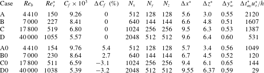
Flow parameters for square duct DNS. The box dimension is
 $6\unicode[STIX]{x03C0}h\times 2h\times 2h$
for all flow cases.
 $Re_{b}=2hu_{b}/\unicode[STIX]{x1D708}$
is the bulk Reynolds number, and
 $Re_{\unicode[STIX]{x1D70F}}^{\ast }=hu_{\unicode[STIX]{x1D70F}}^{\ast }/\unicode[STIX]{x1D708}$
is the friction Reynolds number.
 $\unicode[STIX]{x0394}x$
is the mesh spacing in the streamwise direction, and
 $\unicode[STIX]{x0394}z$
,
 $\unicode[STIX]{x0394}y_{w}$
are the maximum and minimum mesh spacings in the cross-stream direction, all given in global wall units,
 $\unicode[STIX]{x1D6FF}_{v}^{\ast }=\unicode[STIX]{x1D708}/u_{\unicode[STIX]{x1D70F}}^{\ast }$
.
 $\unicode[STIX]{x0394}t_{av}^{\ast }$
is the effective averaging time interval. Flow cases denoted with the 0 suffix are carried out by suppressing the secondary motions.
 $\unicode[STIX]{x0394}C_{f}$
(%) denotes the percentage friction increase/reduction of flow cases with suppression of secondary motions with respect to the reference ones.

This study mainly relies on the DNS database developed by Pirozzoli et al. (Reference Pirozzoli, Modesti, Orlandi and Grasso2018). The compressible Navier–Stokes equations are solved using a fourth-order co-located finite difference solver (Modesti & Pirozzoli Reference Modesti and Pirozzoli2018), and integrated over very long time intervals to guarantee statistical convergence. Four simulations have been carried out at low bulk Mach number,
 $M_{b}=0.2$
, in the range of bulk Reynolds number
 $Re_{b}=4410{-}40\,000$
(
 $Re_{b}=2hu_{b}/\unicode[STIX]{x1D708}$
, where
 $h$
is the duct half side length,
 $u_{b}$
the bulk velocity and
 $\unicode[STIX]{x1D708}$
the fluid kinematic viscosity), and labelled as A–D in table 1. A thorough validation was carried out by Pirozzoli et al. (Reference Pirozzoli, Modesti, Orlandi and Grasso2018), showing good agreement between the new dataset and previous incompressible DNS (Pinelli et al.
Reference Pinelli, Uhlmann, Sekimoto and Kawahara2010; Vinuesa et al.
Reference Vinuesa, Noorani, Lozano-Durán, El Khoury, Schlatter, Fischer and Nagib2014). For the sake of clarity, the velocity components in the streamwise and wall-normal directions are denoted as
 $u$
,
 $v$
and
 $w$
, respectively, and the overline symbol is used to indicate statistical averages in the streamwise direction and in time. In the following both local wall units (based on the local friction velocity,
 $u_{\unicode[STIX]{x1D70F}}=\sqrt{\unicode[STIX]{x1D70F}_{w}/\unicode[STIX]{x1D70C}}$
, with
 $\unicode[STIX]{x1D70F}_{w}$
the local wall shear stress and
 $\unicode[STIX]{x1D70C}$
the density of the fluid) and global wall units (based on the mean shear stress) are used and are denoted with
 $(.)^{+}$
and
 $(.)^{\ast }$
, respectively.
Additional numerical experiments have been carried out here at the same bulk Reynolds numbers as the baseline cases (and denoted with the 0 suffix in table 1), by artificially suppressing the secondary motions. For that purpose we force the streamwise-averaged cross-stream velocity components to have zero mean by setting
 $$\begin{eqnarray}\displaystyle v(x,y,z,t) & \rightarrow & \displaystyle v(x,y,z,t)-\overline{v}^{x}(y,z,t),\end{eqnarray}$$
 $$\begin{eqnarray}\displaystyle w(x,y,z,t) & \rightarrow & \displaystyle w(x,y,z,t)-\overline{w}^{x}(y,z,t),\end{eqnarray}$$
 $\overline{(.)}^{x}$
denotes the streamwise averaging operator. Note that this procedure is independent of the streamwise length of the computational domain or the Reynolds number, as by definition the modified velocities have zero mean, hence the secondary motions are suppressed to machine accuracy. Although the modified velocity field does not strictly satisfy the Navier–Stokes equations, the resulting statistics may be instructive to understand the role of the secondary motions. Previous studies (Pinelli et al.
Reference Pinelli, Uhlmann, Sekimoto and Kawahara2010; Vinuesa et al.
Reference Vinuesa, Noorani, Lozano-Durán, El Khoury, Schlatter, Fischer and Nagib2014) highlighted the need for very long averaging times, thus we have collected flow statistics for equivalent times
 $\unicode[STIX]{x0394}t_{av}^{\ast }=\unicode[STIX]{x0394}t_{av}L_{x}/(6h)$
where
 $L_{x}$
is the streamwise length of the domain (Vinuesa et al.
Reference Vinuesa, Prus, Schlatter and Nagib2016), which are considerably longer than for canonical plane channel flow. On the other hand, we have found that numerical experiments carried out without secondary motions require much shorter time averaging intervals as a result of the suppression of the slow dynamics associated with the secondary currents.
3 The role of secondary motions
In order to quantify the effect of secondary motions on momentum redistribution, we derive a generalized version of the FIK identity (Fukagata et al. Reference Fukagata, Iwamoto and Kasagi2002) for ducts with arbitrary shape. For that purpose we consider the mean streamwise momentum balance equation, namely
 $$\begin{eqnarray}\unicode[STIX]{x1D708}\unicode[STIX]{x1D6FB}^{2}\overline{u}=\unicode[STIX]{x1D735}\boldsymbol{\cdot }\unicode[STIX]{x1D749}_{C}+\unicode[STIX]{x1D735}\boldsymbol{\cdot }\unicode[STIX]{x1D749}_{T}-\overline{\unicode[STIX]{x1D6F1}},\end{eqnarray}$$
where
 $\overline{u}$
is the mean streamwise velocity,
 $\unicode[STIX]{x1D749}_{C}=\overline{u}\,\overline{\boldsymbol{u}}_{yz}$
is associated with mean cross-stream convection (hence, with the secondary motions),
 $\unicode[STIX]{x1D749}_{T}=\overline{u^{\prime }\boldsymbol{u}^{\prime }}_{yz}$
is associated with turbulence convection,
 $\boldsymbol{u}_{yz}=(v,w)$
is the cross-stream velocity vector,
 $\overline{\unicode[STIX]{x1D6F1}}=P\unicode[STIX]{x1D70F}_{w}^{\ast }/(\unicode[STIX]{x1D70C}A)$
is the driving pressure gradient, and
 $A$
and
 $P$
are the duct cross-sectional area and perimeter, respectively. Equation (3.1) may be interpreted as a Poisson equation for the mean streamwise velocity, with source terms
 $\unicode[STIX]{x1D735}\boldsymbol{\cdot }\unicode[STIX]{x1D749}_{T}$
,
 $\unicode[STIX]{x1D735}\boldsymbol{\cdot }\unicode[STIX]{x1D749}_{C}$
and
 $\overline{\unicode[STIX]{x1D6F1}}$
obtained from the DNS dataset. Hence, the solution of (3.1) may be cast as the superposition of three parts, namely
 $\overline{u}=\overline{u}_{V}+\overline{u}_{T}+\overline{u}_{C}$
, with
 $$\begin{eqnarray}\unicode[STIX]{x1D708}\unicode[STIX]{x1D6FB}^{2}\overline{u}_{V}=-\overline{\unicode[STIX]{x1D6F1}},\quad \unicode[STIX]{x1D708}\unicode[STIX]{x1D6FB}^{2}\overline{u}_{T}=\unicode[STIX]{x1D735}\boldsymbol{\cdot }\unicode[STIX]{x1D749}_{T},\quad \unicode[STIX]{x1D708}\unicode[STIX]{x1D6FB}^{2}\overline{u}_{C}=\unicode[STIX]{x1D735}\boldsymbol{\cdot }\unicode[STIX]{x1D749}_{C},\end{eqnarray}$$
with homogeneous boundary conditions, where
 $\overline{u}_{V}$
,
 $\overline{u}_{T}$
and
 $\overline{u}_{C}$
denote the viscous, turbulent and convective contributions to the mean streamwise velocity field. The bulk velocity in the duct may accordingly be evaluated as
 $$\begin{eqnarray}u_{b}=\frac{\overline{\unicode[STIX]{x1D6F1}}A}{\unicode[STIX]{x1D708}}{u_{b}}_{1}+{u_{b}}_{T}+{u_{b}}_{C},\quad {u_{b}}_{X}=\frac{1}{A}\int _{A}\overline{u}_{X}\,\text{d}A,\end{eqnarray}$$
where we have introduced the unitary Stokes velocity field
 $u_{1}$
defined as solution of
 $\unicode[STIX]{x1D6FB}^{2}u_{1}=-1/A$
, which by construction is only a function of the duct geometry, and whereby the viscous velocity field may be expressed as
 $u_{V}=\overline{\unicode[STIX]{x1D6F1}}Au_{1}/\unicode[STIX]{x1D708}$
. Explicit analytical expressions for
 ${u_{b}}_{T}$
were derived by Sbragaglia & Sugiyama (Reference Sbragaglia and Sugiyama2007) in terms of convolution of the turbulence terms with the Stokes velocity field, which do not require the introduction of
 $\overline{u}_{T}$
. Inserting the friction coefficient
 $C_{f}=\overline{\unicode[STIX]{x1D6F1}}D/(2u_{b}^{2})$
(where
 $D=4A/P$
is the duct hydraulic diameter) into (3.3) one obtains
 $$\begin{eqnarray}C_{f}=\frac{2}{{u_{b}}_{1}Re_{P}}\left(1-\frac{{u_{b}}_{T}}{u_{b}}-\frac{{u_{b}}_{C}}{u_{b}}\right)={C_{f}}_{V}+{C_{f}}_{T}+{C_{f}}_{C},\end{eqnarray}$$
where
 $Re_{P}=u_{b}P/\unicode[STIX]{x1D708}$
is the bulk Reynolds number based on the duct perimeter. Equation (3.4) clearly shows that the friction coefficient may be regarded as the sum of the contributions of viscosity, turbulence, and convection (labelled as
 ${C_{f}}_{X}$
), and it directly yields the classical FIK identity in the case of a canonical plane channel and circular pipe flow. However, our formalism has greater generality than the classical FIK identity and its extensions (Peet & Sagaut Reference Peet and Sagaut2009; Jelly, Jung & Zaki Reference Jelly, Jung and Zaki2014), as it further allows one to isolate the effects of mean convection, turbulent and viscous terms on the wall shear stress distributions along the duct perimeter, resulting from
 $$\begin{eqnarray}{\unicode[STIX]{x1D70F}_{w}}_{V}=\unicode[STIX]{x1D70C}\unicode[STIX]{x1D708}\left.\frac{\unicode[STIX]{x2202}\overline{u}_{V}}{\unicode[STIX]{x2202}n}\right|_{w},\quad {\unicode[STIX]{x1D70F}_{w}}_{T}=\unicode[STIX]{x1D70C}\unicode[STIX]{x1D708}\left.\frac{\unicode[STIX]{x2202}\overline{u}_{T}}{\unicode[STIX]{x2202}n}\right|_{w},\quad {\unicode[STIX]{x1D70F}_{w}}_{C}=\unicode[STIX]{x1D70C}\unicode[STIX]{x1D708}\left.\frac{\unicode[STIX]{x2202}\overline{u}_{C}}{\unicode[STIX]{x2202}n}\right|_{w},\end{eqnarray}$$
where
 $n$
is the wall-normal direction. Regarding (3.5) it is important to note that only
 ${\unicode[STIX]{x1D70F}_{w}}_{V}$
has non-zero mean, whereas integration of (3.2) for
 $\overline{u}_{C}$
and
 $\overline{u}_{T}$
readily shows that their integrated contributions vanish as
 $\unicode[STIX]{x1D749}_{C}$
and
 $\unicode[STIX]{x1D749}_{T}$
are both zero at walls.

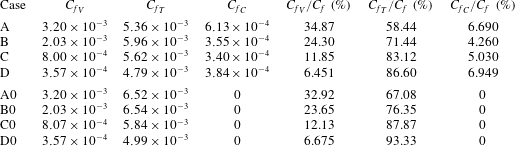
The contributions to the mean friction coefficients are given in table 2, both in absolute terms and as a fraction of the total. Consistent with physical expectations, the viscous contribution is observed to decline at increasing Reynolds number with respect to the turbulent term. The contribution of cross-stream convection is found to be roughly constant across the explored Reynolds number range; however, remaining much less than the turbulence contribution. Extrapolating the DNS data, we expect the convective contribution to exceed the viscous contribution at high enough Reynolds number.
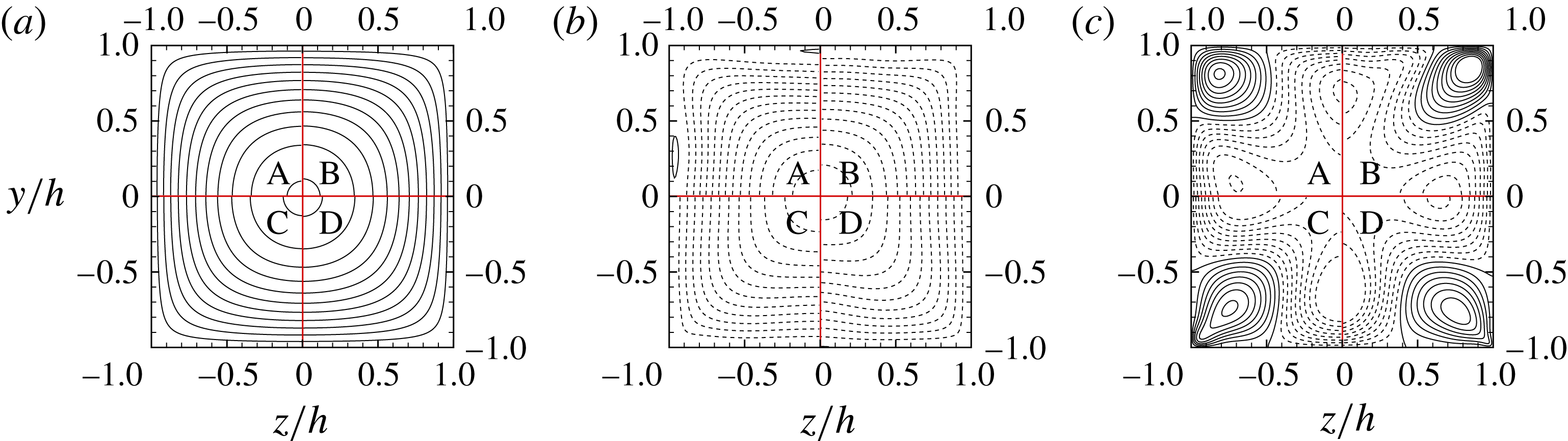
Contributions to mean streamwise velocity
 $\overline{u}$
, each normalized by the corresponding bulk value: viscous
 $\overline{u}_{V}/{u_{b}}_{V}$
(a), turbulent
 $\overline{u}_{T}/|{u_{b}}_{T}|$
(b) and convective
 $\overline{u}_{C}/|{u_{b}}_{C}|$
(c), as defined in (3.2). Data are shown for flow case A (top left), B (top right), C (bottom left), D (bottom right). Contour levels are shown for the range
 $0\leqslant (.)/|{u_{b}}_{X}|\leqslant 2$
in intervals of 2 in (a,b), and for the range
 $-4\leqslant (.)/|{u_{b}}_{C}|\leqslant 4$
in intervals of 0.5 in (c) (dashed lines indicate negative values).

Figure 1 shows the streamwise velocity fields associated with viscous, turbulent and convective terms. For the sake of clarity, each contribution is normalized with the corresponding bulk value,
 ${u_{b}}_{X}$
, where
 ${u_{b}}_{T}$
and
 ${u_{b}}_{C}$
are both negative, hence providing an additive effect to the duct friction (see (3.4)). The viscous-associated velocity field
 $u_{V}$
arises from the solution of a Poisson equation with a uniform right-hand side (the pressure gradient), hence its geometry is identical to the case of Stokes flow (Shah & London Reference Shah and London2014), depending only on the duct cross-sectional geometry. The turbulence-associated velocity field
 $u_{T}$
, shown in figure 1(b), is everywhere negative and topologically similar to the viscous-associated field, highlighting a retarding effect of turbulence on the bulk flow, with an incurred increase of the friction coefficient. The velocity field
 $u_{C}$
induced by mean convection, shown in figure 1(c), has a more complex organization. Positive values are found near the duct corners, whereas negative values are found near the duct bisectors, the zero crossings being located half-way in between. This finding is consistent with the intuitive expectation that secondary motions tend to equalize momentum across the duct cross-section, thus quantitatively corroborating claims made by early investigators (Prandtl Reference Prandtl1926). Notably, the distributions shown in figure 1 are not qualitatively affected by Reynolds number variation when scaled with respect to their mean integral value, thus showing that changing the Reynolds number changes only the relative importance of the three terms, as quantified in table 2.
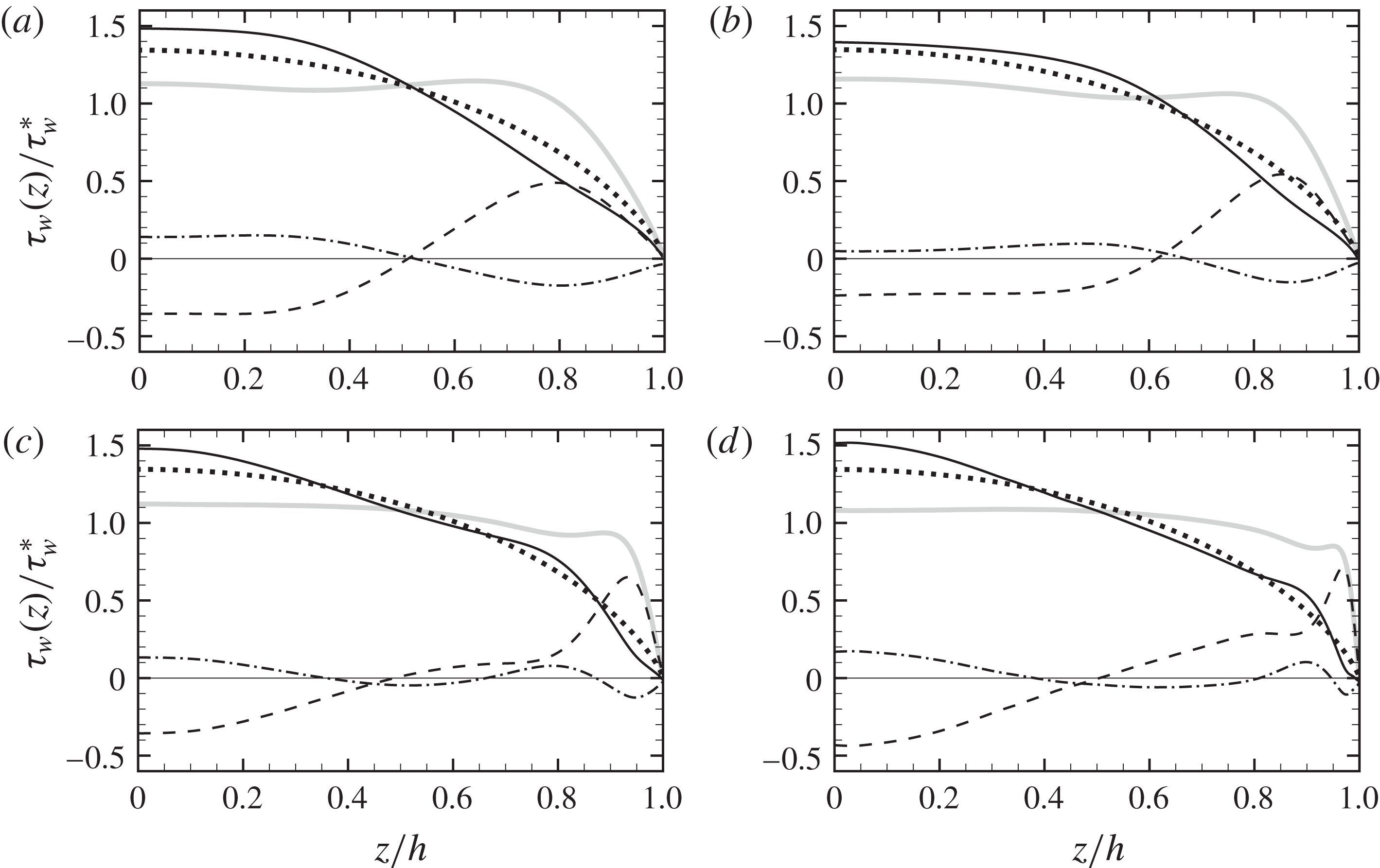
Contributions to mean wall shear stress (shown along a half duct side): viscous (
 ${\unicode[STIX]{x1D70F}_{w}}_{V}(z)$
, dotted), turbulent (
 ${\unicode[STIX]{x1D70F}_{w}}_{T}(z)$
, dash-dotted), viscous
 $+$
turbulent (
 ${\unicode[STIX]{x1D70F}_{w}}_{V}(z)+{\unicode[STIX]{x1D70F}_{w}}_{T}(z)$
, solid), mean convection (
 ${\unicode[STIX]{x1D70F}_{w}}_{C}(z)$
, dashed), and total (
 $\unicode[STIX]{x1D70F}_{w}(z)$
, thick grey) for flow cases A–D in panels (a–d), respectively.

The observations made regarding the organization of the streamwise velocity field have direct impact on the distribution of the local wall shear stress, shown in figure 2. The wall shear stress distribution induced by viscous terms (dots) is the same for all cases, and nearly parabolic in shape. The turbulence terms (dash-dotted lines) have a complex behaviour, exhibiting multiple peaks which change with the Reynolds number. In general, they yield an increase in friction towards the duct bisectors, and slight attenuation at the corners (compare the solid lines with the dotted lines), thus making the wall friction distributions more non-uniform. Mean convection (dashed lines) yields large positive peaks in the vicinity of the corners, whose distance from the neighbouring walls scales in inner units (Pirozzoli et al.
Reference Pirozzoli, Modesti, Orlandi and Grasso2018), and negative values around the duct bisector. As a result, the distributions of the wall shear stress (thick grey lines) tend to be rather flat – especially at high enough Reynolds number. This behaviour is consistent with recent theoretical analysis based on inner–outer layer matching arguments (Spalart, Garbaruk & Stabnikov Reference Spalart, Garbaruk and Stabnikov2018), which suggest that only uniform wall shear stress along the duct perimeter is compatible with the formation of logarithmic layers of the mean streamwise velocity in the asymptotic high-
 $Re$
regime.
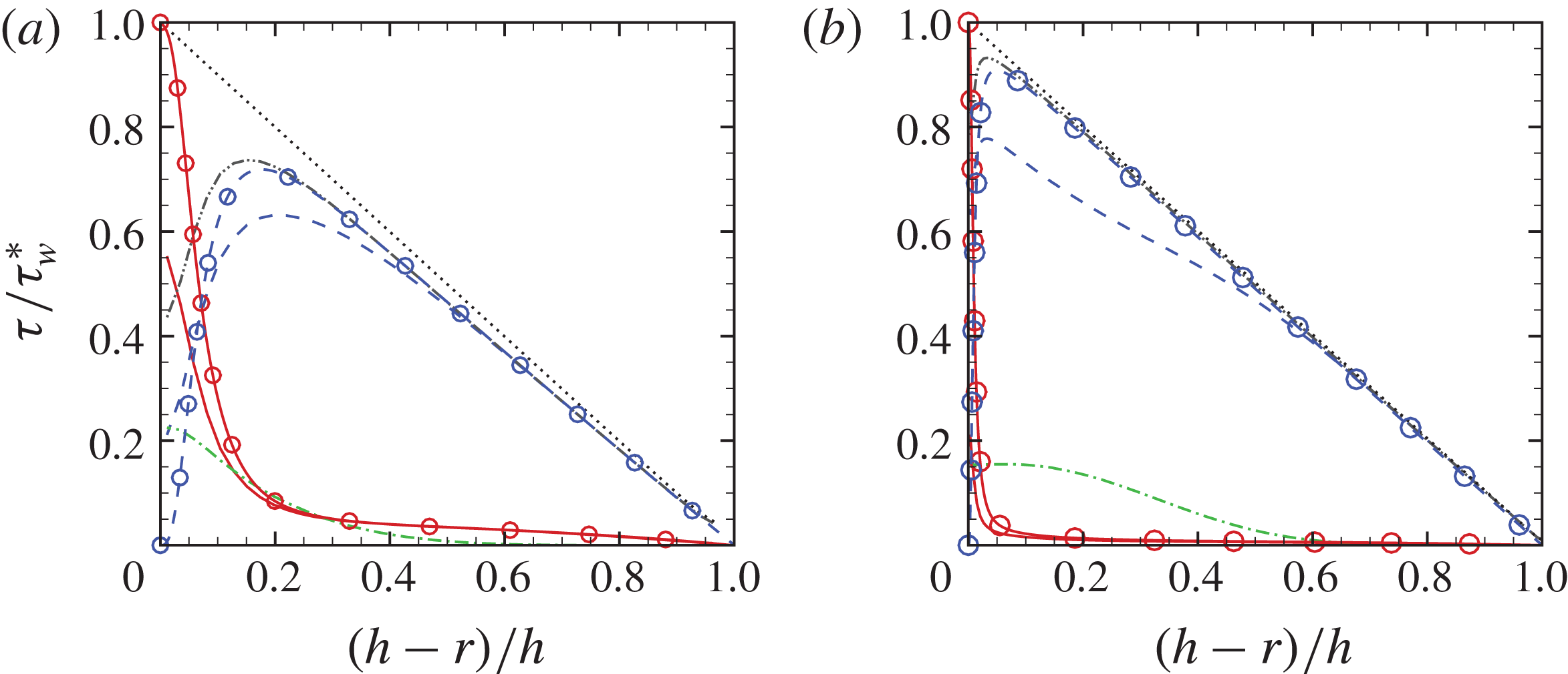
Profiles of azimuthally averaged stresses for flow case A (a) and flow case D (b) as a function of the distance from the duct centre (
 $r$
), as defined in (3.6): viscous
 $\unicode[STIX]{x1D70F}_{V}$
, solid; turbulent
 $\unicode[STIX]{x1D70F}_{T}$
, dashed; convective
 $\unicode[STIX]{x1D70F}_{C}$
, dash-dotted; turbulent
 $+$
convective
 $\unicode[STIX]{x1D70F}_{T}+\unicode[STIX]{x1D70F}_{C}$
, dash-dot-dot; total stress
 $\unicode[STIX]{x1D70F}_{t}$
, dotted. Circles denote pipe flow data (Wu & Moin Reference Wu and Moin2008) at
 $Re_{\unicode[STIX]{x1D70F}}=180$
(a) and
 $Re_{\unicode[STIX]{x1D70F}}=1140$
(b).

The role of the secondary motions is further analysed using the mean momentum balance equation (3.1), averaged over circular shells. Let
 $r$
,
 $\unicode[STIX]{x1D703}$
be polar coordinates about the duct centre; it is a simple matter to show that integrating (3.1) along the radial direction yields the counterpart of the law of linear variation of the total stress with the wall distance in canonical flows, namely
 $$\begin{eqnarray}\unicode[STIX]{x1D70F}_{t}(r)=\unicode[STIX]{x1D70F}_{V}(r)+\unicode[STIX]{x1D70F}_{C}(r)+\unicode[STIX]{x1D70F}_{T}(r)=\unicode[STIX]{x1D70F}_{w}^{\ast }r/h,\quad \unicode[STIX]{x1D70F}_{X}=1/r\int _{0}^{r}\unicode[STIX]{x1D70C}\langle \unicode[STIX]{x1D735}\boldsymbol{\cdot }\unicode[STIX]{x1D749}_{X}\rangle _{\unicode[STIX]{x1D703}}\,\text{d}\unicode[STIX]{x1D70C},\end{eqnarray}$$
where
 $r$
is the radial distance from the duct centre, the local stresses
 $\unicode[STIX]{x1D749}_{X}$
are defined in (3.1), and
 $\langle \rangle _{\unicode[STIX]{x1D703}}$
denotes the averaging operator in the azimuthal direction. Equation (3.6) holds for
 $r\leqslant h$
, the upper limit corresponding to the condition of tangency of circular shells with the duct walls. The terms
 $\unicode[STIX]{x1D70F}_{X}$
represent the viscous, turbulent and convective stresses averaged in the azimuthal direction, and according to (3.6) their sum is supposed to vary linearly with the radial coordinate. Figure 3 shows the distributions of the averaged stresses as a function of nearest wall distance,
 $h-r$
. Mean momentum balance is satisfied with very good accuracy, as the distributions of the total stress (dotted lines) are very nearly linear. Interestingly, the distributions of the total stress components are very similar to those observed in pipe flow, also shown for reference. Specifically, the viscous stress (solid lines) increases towards the wall; however, its value is much less than
 $\unicode[STIX]{x1D70F}_{w}^{\ast }$
, because averaging in the
 $\unicode[STIX]{x1D703}$
direction also collects points far from walls where the viscous stress is very small. The turbulent stress (dashed lines) has an opposite behaviour, being dominant away from walls, and non-zero for
 $r\rightarrow h$
, again on account of the
 $\unicode[STIX]{x1D703}$
averaging. The convective stress (dash-dotted lines) is far from negligible, especially near walls, and its relative importance increases with the Reynolds number. Comparing with flow statistics from pipe DNS (Wu & Moin Reference Wu and Moin2008), we find that when convective and turbulent stresses are taken together (dash-dot-dotted line), good collapse of the stresses is achieved starting from a wall distance of approximately
 $0.3h$
. Bearing in mind that non-uniformities in the
 $\unicode[STIX]{x1D703}$
direction have been removed through the averaging procedure, this observation probably points to a universal structure of all duct flows, which corroborates the validity of Townsend’s outer layer similarity hypothesis (Townsend Reference Townsend1976) also in non-canonical flows. Similar conclusions were drawn by Marin et al. (Reference Marin, Vinuesa, Obabko and Schlatter2016), who pointed out the similarity between the azimuthal velocity variances in hexagonal duct and pipe flow in the core region of the two flows.
4 Suppression of secondary motions
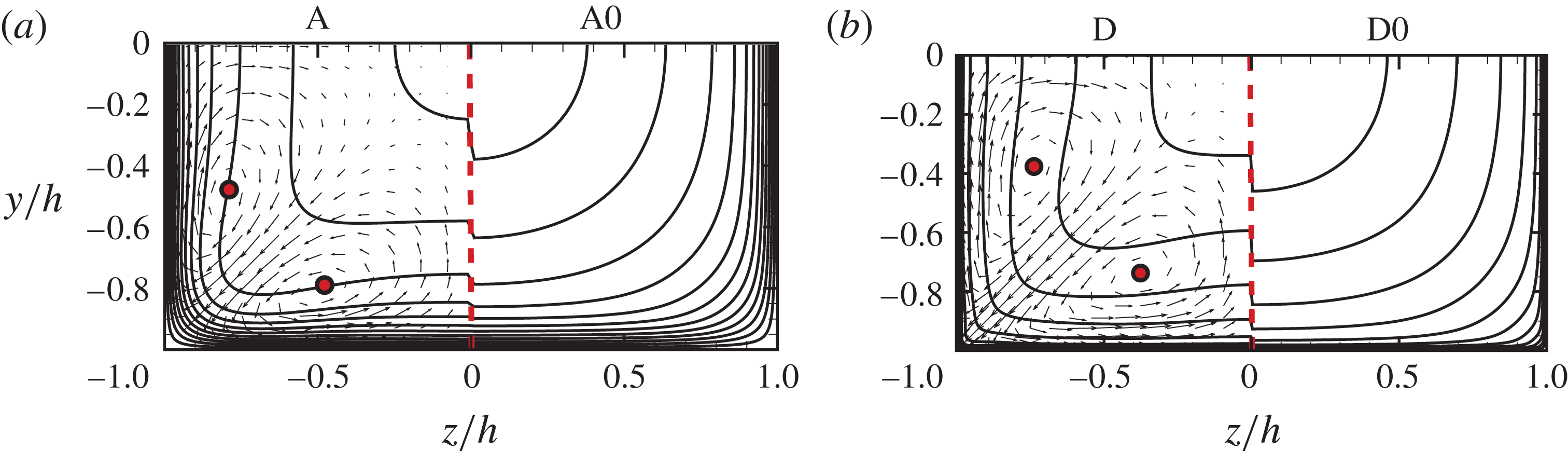
Mean streamwise velocity contours and cross-stream velocity vectors with (left) and without (right) secondary motions for flow cases A–A0 (a) and D–D0 (b). Thirteen contour levels are shown in the range
 $0\leqslant \overline{u}/u_{b}\leqslant 1.3$
. The circles mark the centres of the secondary eddies.

Numerical experiments with artificial suppression of the secondary motions (flow cases A0–D0) are here compared with full DNS (flow cases A–D). In figure 4 we show mean streamwise velocity contours in cross-stream planes. Upon suppression of the secondary motions, the flow no longer exhibits the typical bulging of the velocity isolines, because momentum transfer from the duct core towards the corners is inhibited. In practical terms, this qualitative change is not accompanied by a substantial variation of drag, and indeed table 1 shows a modest drag increase for flow cases A0–B0, and a modest drag decrease for flow cases C0–D0. We argue that this non-monotonic behaviour is due to the displacement of the centroids of the secondary eddies in the low-Reynolds-number post-transitional regime (see Pirozzoli et al. (Reference Pirozzoli, Modesti, Orlandi and Grasso2018, figure 18)).
The analysis of the contributions to the total friction carried out in § 3 has been repeated for the flow cases without secondary motions, and the results are reported in table 2 for flow cases A0–D0. It appears that the viscous contribution is very nearly the same as in the baseline cases, and the absence of convection is almost entirely compensated for by an increase of the turbulent contribution, in such a way that the overall variation of friction is quite small.
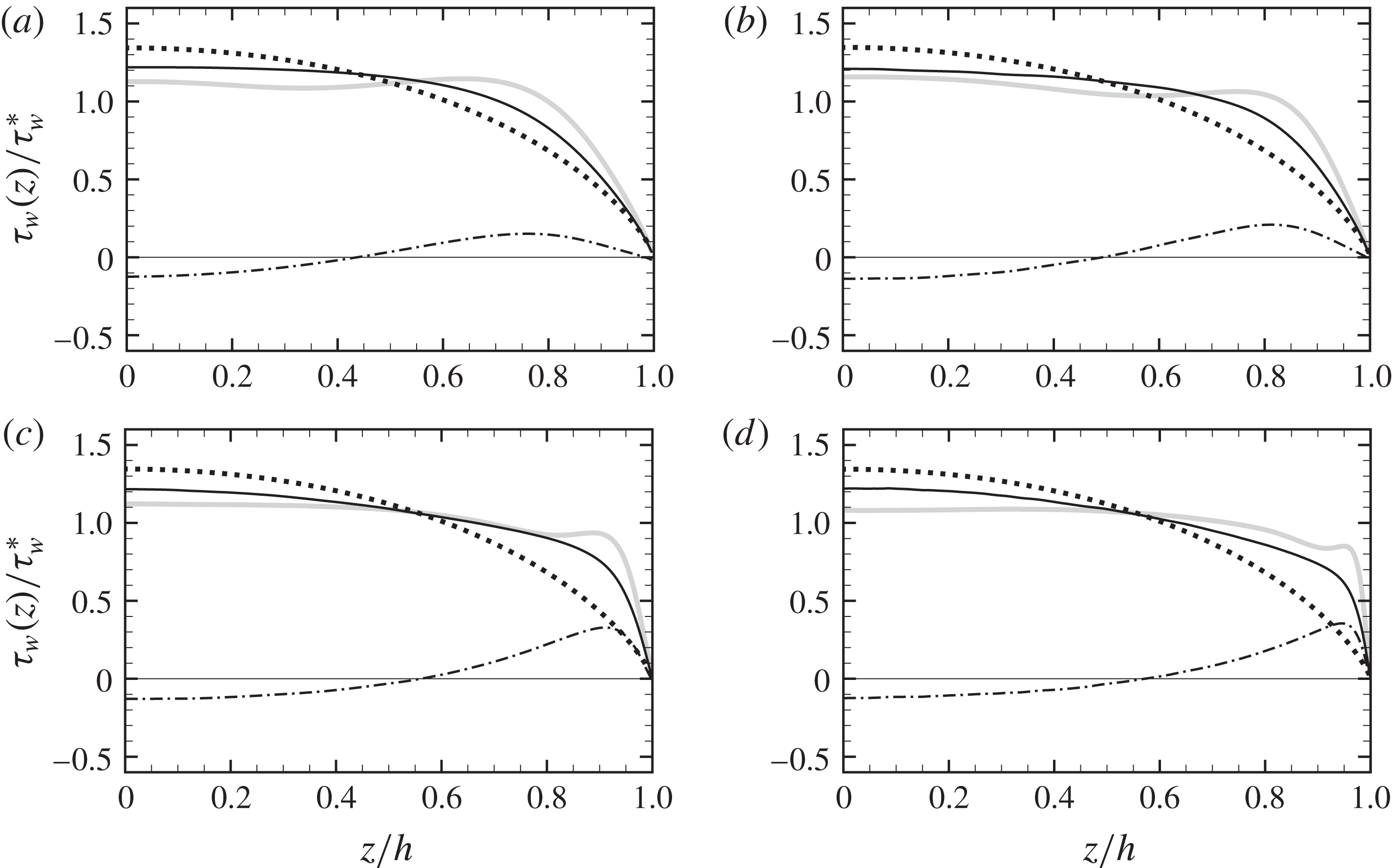
Contributions to mean wall shear stress (shown along a half duct side): viscous (
 ${\unicode[STIX]{x1D70F}_{w}}_{V}(z)$
, dotted), turbulent (
 ${\unicode[STIX]{x1D70F}_{w}}_{T}(z)$
, dash-dotted), and total (
 $\unicode[STIX]{x1D70F}_{w}(z)$
, solid) for flow cases A0–D0 in panels (a–d), respectively. The wall shear stress for flow cases A–D is also shown for comparison as thick grey lines in the corresponding panels.

The distributions of the wall shear stress for flow cases A0–D0 are shown in figure 5. Overall, the wall shear stress (solid lines) is less flat than in flow cases A–D (grey lines), and it no longer exhibits the typical near-wall peaks caused by mean convection (see also figure 2). Comparison with figure 2 shows that the viscous contribution obviously retains the same shape, whereas the turbulence contribution is qualitatively modified by suppression of the secondary motions. In particular,
 ${\unicode[STIX]{x1D70F}_{w}}_{T}$
(dash-dotted lines) has reversed sign, becoming positive towards the corners and negative at the duct mid-side, thus partially replacing cross-stream convection. This observation is consistent with the fact that the associated velocity field (not shown) has a structure similar to the convection term in figure 1(c), thus bringing high-momentum fluid towards the corners. This behaviour further suggests that secondary motions are a manifestation of turbulence and, upon suppression of the mean convection, the Reynolds stresses act to restore the mean momentum balance.
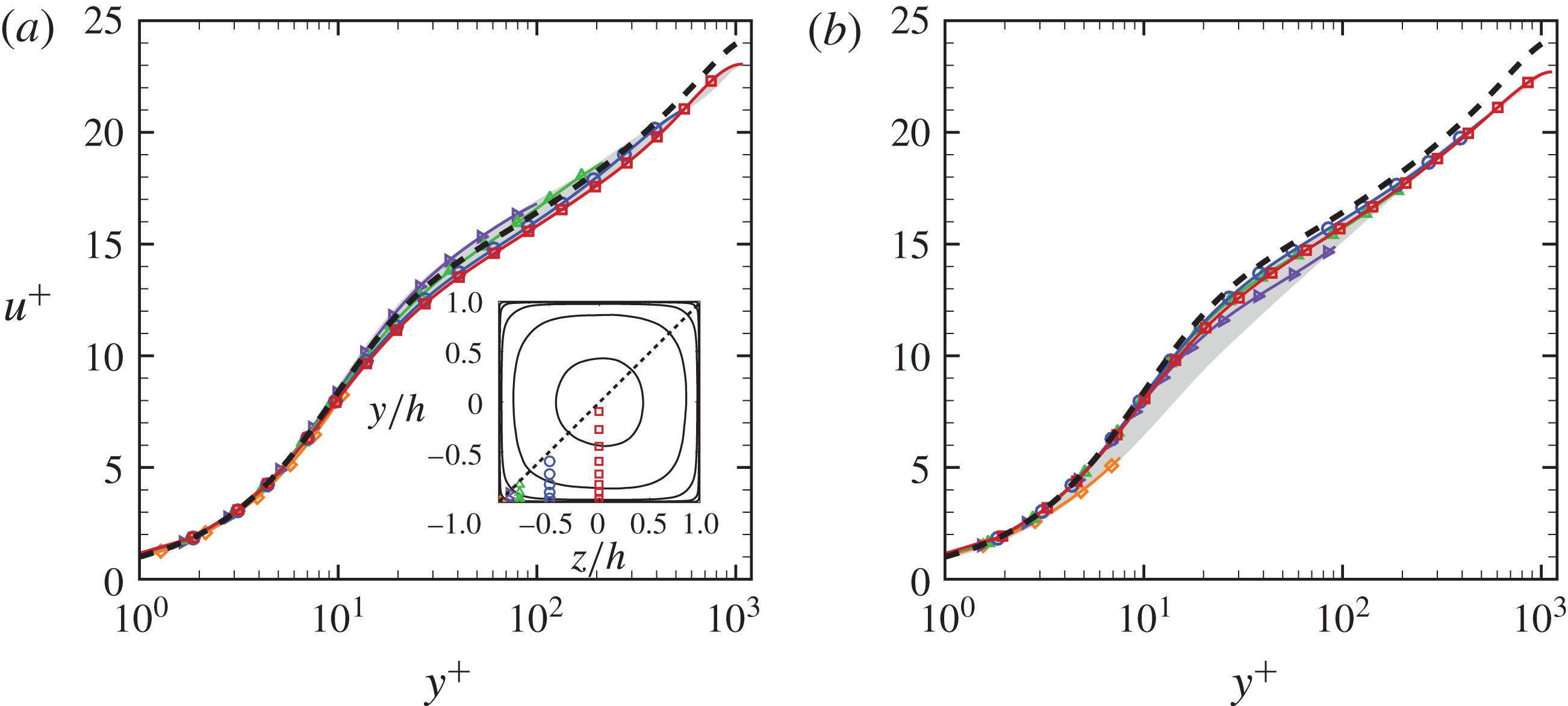
Mean streamwise velocity profiles along the wall-normal
 $y$
direction, given in local wall units at all
 $z$
up to the corner bisector, for flow cases D and D0 in (a) and (b), respectively. Representative stations along the bottom wall are highlighted, namely
 $(z+h)=15\unicode[STIX]{x1D6FF}_{v}^{\ast }$
(diamonds),
 $(z+h)/h=0.1$
(right triangles),
 $(z+h)/h=0.25$
(triangles),
 $(z+h)/h=0.5$
(circles),
 $(z+h)/h=1$
(squares), see inset in (a). The dashed lines denote profiles from DNS of pipe flow at
 $Re_{\unicode[STIX]{x1D70F}}=1140$
(Wu & Moin Reference Wu and Moin2008).

The inner-scaled wall-normal mean velocity profiles are shown in figure 6 for the highest Reynolds number cases. For the sake of clarity, the profiles are scaled in local wall units at each
 $z$
location along the bottom wall, and shown up to the corner bisector
 $y=z$
(see inset in panel a), where velocity has local maxima. The mean velocity profiles for circular pipe flow (Wu & Moin Reference Wu and Moin2008) are also included for comparison. As pointed out by Pirozzoli et al. (Reference Pirozzoli, Modesti, Orlandi and Grasso2018), local wall scaling yields excellent collapse of the velocity distributions up to the corner bisector, thus supporting the robustness of the law of the wall in wall-bounded turbulence. However, removing the secondary motions (panel b) yields greater data scatter in the buffer layer, and deviations from the pipe velocity profile are consequently larger also in the outer layer. In this respect we again recall that the analysis of Spalart et al. (Reference Spalart, Garbaruk and Stabnikov2018) shows that a log law can only be achieved in ducts with complex cross-section if the wall shear is uniform. Hence, the observed greater universality of the inner-scaled velocity profiles in the presence of secondary motions is likely to be the side result of greater uniformity in the wall shear stress distributions. In this sense, we may further state that secondary motions contribute to establishing universality of the flow statistics.
5 Conclusions
Based on the results of this study, we are in a position to make a judgement about the actual effect of secondary motions on the flow statistics, thus providing quantitative answers to a frequently debated subject. As regards the bulk flow properties, we find that secondary motions contribute as much as 6 % to the mean duct friction coefficient, hence their suppression may in principle yield some relief in terms of a reduced pressure drop. This expectation is not realized in practice, and we find that artificially suppressing the secondary motions changes the structure of the turbulence terms in a partially compensating fashion. Hence, a drag increase is found at low Reynolds number, and a drag reduction of no more than 3 %, at sufficiently high Reynolds number. Notably, this drag reduction is comparable to that obtained with a change of duct shape from square to circular. Indeed, assuming that friction is controlled by the Reynolds number based on the hydraulic diameter, and considering for simplicity the Blasius friction law, namely
 $C_{f}=0.079Re_{D}^{-1/4}$
, it is easily found that the ratio of the friction coefficient in a square duct as compared with a circular pipe with the same area is
 $(2/\sqrt{\unicode[STIX]{x03C0}})^{1/4}\approx 1.03$
.
As regards the general flow organization, we are able to quantitatively confirm that the main role of the secondary motions is to bring high-momentum fluid from the side bisectors towards the corners, hence tending to compensate the momentum defect at the duct corners and to make for a fuller mean velocity profile, thus counteracting non-uniformities induced by the viscous and turbulence terms. As a result, the distributions of the wall shear stress also tend to be more uniform than would be obtained if only the viscous and turbulence terms were retained. Artificial suppression of the secondary motions changes the qualitative structure of the turbulence terms, which then assume a uniforming role similar to mean convection, thus suggesting that secondary motions are an intrinsic mechanism of turbulence, which acts to restore uniform wall scaling. However, the wall shear stress distributions are less flat than in the case of the full DNS. As a result, DNS including the secondary motions tend to have greater universality of the wall-normal mean velocity profiles, which follow with good fidelity the canonical log law.
A further outcome of the present analysis is that the azimuthally averaged mean momentum budget terms reveals a structure similar to that found in circular pipe flow, thus supporting the extended validity of Townsend’s similarity hypothesis also for flows in ducts with complex shape. In the presence of secondary motions, mean convection provides a contribution comparable to the turbulent stresses, especially near the walls, which however adds to the turbulent contribution, yielding an effective averaged stress distribution which is very similar to pipe flow.
Acknowledgements
We acknowledge support from J. Jimenez for hosting us during the Third Madrid Turbulence Workshop, funded by the COTURB ERC project. We further acknowledge that the data reported in this paper have been computed using the PRACE Research Infrastructure resource MARCONI based at CINECA, Casalecchio di Reno, Italy.