Nomenclature
- AoA
-
angle-of-attack
- AoY
-
angle-of-yaw
- APU
-
auxilirary power unit
- CHARME
-
CHallenge AéRoMEchanique
- D
-
characteristic dimmension [m]
- DGAC
-
Direction Générale de l’Aviation Civile
- g
-
Earth’s surface standard gravitational acceleration [m/s
 $^2$
]
- H/C
-
helicopter
- LSD
-
Linear Spectral Density
- PIV
-
Particle Image Velocimetry
- PSD
-
Power Spectral Density
- PU
-
Power Unit
- Q
-
mass flow at the APU air intake [kg/s]
- Re
-
Reynolds number [–]
- RMS
-
Root Mean Square
- St
-
Strouhal Number [–]
- U
-
flow velocity longitudinal component [m/s]
- V
-
flow velocity lateral component [m/s]
-
${V_h}$
-
maximum level-flight speed [m/s]
-
${V_y}$
-
best rate-of-climb speed [m/s]
- W
-
flow velocity vertical component [m/s]
- WTT
-
Wind-Tunnel Tests


Greek symbol
-
$\kappa $
-
inverse of the WTT scale ratio [–]

Indices
- FS
full scale
- WT
wind-tunnel scale
1.0 Introduction
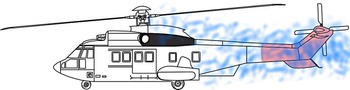
Tail-shake is commonly defined as the vibratory response of the overall helicopter structure throughout its elastic eigenmodes to aerodynamic excitations of the tail parts [Reference Cassier, Weneckers and Pouradier1]. Tail-shake has historically been identified as strong interactions between the wakes emitted from the main-rotor assembly and/or flow separations over the fuselage, and the impinged areas at the tail unit in forward flight [Reference Sheridan and Smith2], as illustrated in Fig. 1.
The sources of wake vary from one platform to another. Nonetheless, for conventional helicopters, the most frequent influencing factors are the flight conditions, the rotor rotational speed and of course the design of some critical components, e.g. the main rotor hub, the upper deck [Reference Roesch and Dequin3], the rear-ramp angle, the architecture of the bottom parts (skids, cross-tubes or wheels), the implementation of optionals, additional air inlets/outlets, as well as the proximity of the rotor to the fuselage [Reference De Waard and Trouvé4].
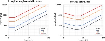
The resulting low-frequency vibrations in the cabin often exhibit erratic lateral-or-vertical kicks that must be endured by the crew and passengers [Reference Cassier, Weneckers and Pouradier1]. The discomfort caused by those vibrations depends of course on their characteristic frequencies and magnitudes, but also on the vibration direction, the point of contact with the body, and the duration of vibration exposure. The International Standard 2,631 (ISO 1974, 1985, 1997) defines exposure limits, which are set approximately at half the level considered to be the threshold of pain for healthy human subjects, as illustrated in Fig. 2. Vibrations induced by tail-shake typically occur between 5 and 20Hz, with peak amplitudes greater than
 $0.1g$
at the pilot seats [Reference Roesch and Vuillet5], thus corresponding to a frequency range where humans are particularly sensitive, and to magnitudes preventing from long daily exposure [Reference Griffith6].
Schematic illustration of the tail-shake phenomenon in forward flight; in blue: wake; in red: impingement areas.

ISO 2631 daily exposure limits for human response to whole-body vibrations; amplitudes in % of the Earth’s surface standard gravitational acceleration g. Left: Longitudinal/lateral vibrations. Right: Vertical vibrations, from Ref. (Reference Griffith6).

Whole-body vibrations can also impair the acquisition of information (e.g. by the eyes), the output of information (e.g. by hand or foot movements) or the complex central processes that relate inputs to outputs (e.g. decision-making) [Reference Griffith6]. As an example, in some critical situations, tail-shake vibrations may increase the pilot workload, e.g. the dashboard may become difficult to read. They might also damage onboard equipment. Of course, tail-shake is not the unique source of vibrations in cabin, but it may be a major source of discomfort in some particular flight conditions, e.g. in cruise or descent flight. This is why tail-shake has to be prevented.
Tail parts are straightforward components that are involved in the tail-shake phenomenon. Nonetheless, the upper deck may also play a major role for the following reasons:
The engine cowlings may be the origin of large flow separations especially in high-pitch situations [Reference Roesch and Dequin3]. Large vortices are thus shed and may impinge the tail unit after a long convection with potential non-linear interactions with wakes emitted by other systems.
Pylon fairings are principally aimed at limiting the drag generated by the rotor hub and improving the tail-parts efficiency; the rotor mast, the swashplate, the control rods and the scissors are partially or totally shielded thus avoiding major aerodynamic interactions of those components with the tail unit [Reference Graham, Sung, Young, Louie and Stroub7]. But as comprehensively described by Roesch and Vuillet [Reference Roesch and Vuillet5], pylon fairings may also be smartly designed so as to mitigate flow separations at the aft cowlings, and tail-shake risks as a side effect. Indeed, thanks to the protruding lips at the pylon-fairing sides – as implemented on almost all the range of Airbus Helicopters products – the airstream approaching the pylon deck is deflected upwards and escapes laterally around the lips into tip vortices. These vortices exert a suction effect on the air flowing past the side of the pylon fairing. The pair of vortices also produces a suction effect on the wake which follows the aft portion of the pylon fairing [Reference Roesch and Vuillet5]. In addition, counter-rotating lip vortices tend to counterbalance any lateral deviations of the flow at the aft cowlings. The consequence is usually delayed flow separations, along with an increased robustness of the cowlings to a change of pitch or yaw angles regarding flow attachment.
Several air inlets are usually implemented on helicopter upper deck; those are of course the intakes of engines or power units (PU) but also inlets ensuring cooling functions such as oil cooling, air cooling in cabin etc. Depending on their locations, shapes and associated mass flows, they may alter the favourable aerodynamic behaviour of the pylon fairing regarding tail-shake, and/or induce flow separations at the cowlings. Installation losses, reingestion and performance aspects remain obviously the key drivers in the implementation of air intakes, but the aforementioned elements also invite to consider the air-intake locations with care regarding tail-shake.
Inflight rotor/airframe/flow interactions at the origin of the tail-shake phenomenon remain particularly challenging to predict with confidence before maiden flights of a new helicopter. Historically, redesign loops relying on Wind-Tunnel Test campaigns had to be conducted during prototyping phases, as reported for SA365N [Reference Roesch and Vuillet5], Tiger [Reference Cassier, Weneckers and Pouradier1], NH90 [Reference Hakkaart8, Reference Hermans, Hakkaart and Hegen9] or EC135 [Reference Kampa, Enenkl, Polz and Roth10], because of the lack of highly accurate prediction methods for tail-shake during the predesign phase. Late redesign loops usually entail additional development costs along with an increased time to market that could jeopardise the profitability of a new development. That’s why they have to be avoided. As a consequence, and despite some representativeness limitations (missing rotors, unreliable dynamic response of the airframe), wind-tunnel tests still play an important role in the tail-shake derisking process. Indeed, they allow:
-
• identifying critical flight configurations which present a potential tail-shake hazard;
-
• drawing the general trends and define suitable airframe design modifications, by ranking numerous shapes at a reasonable cost based on the evaluation of unsteady characteristics of the flow;
-
• producing databases to mature and improve numerical models, which become more and more promising [Reference Schäferlein, Keßler and Krämer11].
In this work, the role of the upper deck – including the air intakes installed on it – as a potential source of tail-shake is investigated. The study relies on a wind-tunnel test (WTT) campaign as part of a more general development logic regarding tail-shake derisking. The tests have been performed on a mock-up representative of the upper deck of a heavy-weight class helicopter. As the tail-shake risks are characterised at the source, tail parts of mock-ups have been discarded.
2.0 Experimental set-up
2.1 Marignane wind tunnel
The WTT campaign has been conducted at the Airbus Helicopters’ Wind-Tunnel facilities located in Marignane, France. The Marignane Wind Tunnel (WT) is an open return tunnel with a test section of dimension 3m (diameter)
 $ \times $
3m (length). The maximum flow velocity in the test section is 40m/s under atmospheric conditions. The turbulence rate is approx. 3%.
2.2 Tested parts
2.2.1 Fuselage
An unpowered mock-up representing a generic heavy helicopter fuselage has been considered. The model has been downscaled to scale 1:3.5. The large scale has been mandatory to prevent from a significant reduction of the Reynolds number with respect to full scale, as well as to ensure a representative PU air-intake design. The upper-deck representativeness is also mandatory in order to feed the aft pylon fairing with a high-fidelity-inflected incoming flow. No tail-boom nor tail parts are implemented on the model. In addition, in order to isolate the wake generation to evaluate, no rotor head nor lower parts have been considered. The main-engine intakes and exhausts are plugged. The rotor cavity at the pylon fairing remains also always plugged during the whole campaign.
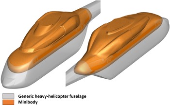
A minibody has been chosen as the most relevant solution to satisfy the aforementioned constraints. It also allows to maintain the blockage coefficient of the bench test below a reasonable value – typically 10%. At last, the minibody is characterised by a high clearance despite the large scale, which allows to explore a wide range of flight conditions, as the angle-of-attack has been adjustable between
 $ - {12^ \circ }$
and
 $ + {12^ \circ }$
. The minibody geometry roughly consists in considering a half oblate spheroid as a replacement of the nose of the generic heavy-weight helicopter. It ensures a reduction by half of its cell’s height, as depicted in Fig. 3.
Generic heavy-helicopter fuselage and associated minibody.

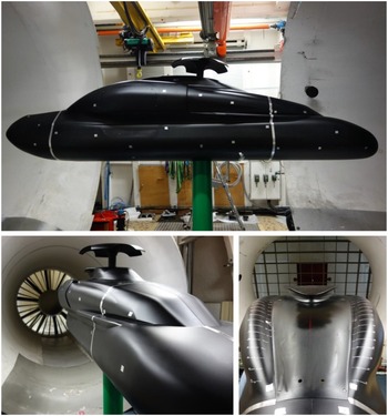
Several design iterations have been needed to converge to a clean design that preserves the representativeness of the flow at the upper deck without any spurious perturbations from the redesign of the nose or the reduction of the cell size. At scale 1:3.5, the minibody is 340cm long and 160cm high. The mock-up is mounted on a 180mm-diameter mast. The whole test bench is shown in Fig. 4.
Overview of the minibody configuration in the Marignane Wind-Tunnel facilities (here with a hub cap).

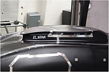
Baseline pylon-fairing shape with no APU air intake (AI_NONE).

2.2.2 Air intakes
Only the air intakes of an auxiliary power unit (APU) are considered in what follows. Indeed, the APU air intake installation on the upper deck represents a significant architectural challenge with a lower maturity level regarding tail-shake than for the main-engine ones. For the latter they are usually tailored for a certain H/C velocity range – typically around the maximum level-flight speed (
 ${V_h}$
) – such that disturbances of the flow are minimal. The main-engine air intakes have thus been plugged on the mock-up. Three different air-intake implementations to supply an APU have been tested. Given the narrow volume available at the upper deck for an additional air intake, the number of possible implementations remains limited, as the intake mouth has to be sufficiently large to ensure low pressure drops in hover.
-
• The baseline pylon-fairing shape with no APU air intake (AI_NONE), as shown in Fig. 5.
-
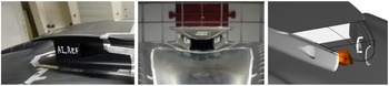
• Air intake #1, implemented at the pylon-fairing trailing edge (AI_REF), as illustrated in Fig. 6. Two NACA inlets have been implemented on the sides so as to improve the efficiency of the intake in advancing conditions.
-
• Air intake #2, implemented upstream of the pylon-fairing lips (AI_BU) on each side of the pylon fairing, close to its maximum cross-section location. This configuration is depicted in Fig. 7. An enlargement of the pylon fairing by 100mm at scale 1:1 on each side has been required to implement the ducts from the inlets to the APU. This type of implementation is more classical but it has several drawbacks, in particular the increase of the H/C empty weight due to the ducts and the larger pylon fairing, along with less efficient air intakes in hover.
2.2.3 Mitigation means
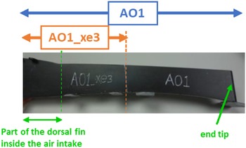
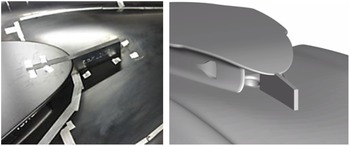
Air intake #1 (AI_REF) has a priori a high probability of disturbing the favourable aerodynamic behaviour of the pylon fairing regarding tail-shake. This is why two mitigation means are proposed. They consist in separating walls of different length to be mounted at the air-intake mouth along the cowling centreline (“dorsal fin”), as patented in EP3395690 [Reference Desvigne12]. Those separating walls are aimed at limiting the interactions between the pylon-fairing lip vortices – which must be kept undisturbed as much as possible – and the suction at the APU air intake. The baseline “dorsal fin” (AO1) is 408mm long, with 90mm inside the air intake. A shortened variant (AO1_xe3) has also been considered, by cutting the long dorsal fin at 45% from the end tip, as illustrated in Fig. 8. Those mitigation means present the advantage of being very easy to implement on the cowlings, together with a limited impact on the H/C empty weight. The short dorsal fin mounted on the mock-up is depicted in Fig. 9.
Air intake #1 (AI_REF) located at the aft portion of the pylon fairing.

Air intake #2 (AI_BU) located on the sides of the pylon fairing. Right: Overview of the enlarged pylon fairing hosting AI_BU (in orange) w.r.t. baseline.

Dorsal fin AO1 before cut; the length limit for the shorter variant AO1_xe3 is delimited by the orange dot line.

Dorsal fin AO1_xe3 i.e. AO1 after cut.

2.3 Operating conditions at full scale
In order to cover all the possible cases of interactions at the upper deck, the APU is tested both in on– and off–mode. Indeed, the additional power produced by the APU may not always be necessary all over the flight envelope. As a consequence, the APU may possibly be switched off during the flight – like in cruise at
 ${V_y}$
– and the case with no air inflow at the intake has to be considered accordingly. The campaign has focused on the flight conditions expected to be the most propitious for tail-shake to appear [Reference Cassier, Weneckers and Pouradier1, Reference Roesch and Vuillet5, Reference Graham, Sung, Young, Louie and Stroub7, Reference Hakkaart8, Reference Hermans, Hakkaart and Hegen9]. Those flight conditions are reported in Table 1. A generic mass flow at the APU air intake is also given.
Typical flight conditions potentially propitious to tail-shake at full scale

2.4 Downscaling the operating conditions
Downscaling the full-scale operating conditions is an important step when preparing the WTT campaign, because the analysis must be portable to the full scale. We propose in this part elements about how the APU mass flow, the scale and the incoming-flow velocity have been selected.
2.4.1 Mass flow at the APU air intake
When the APU operates, for the sake of representativeness, the stream tubes entering the air intake have to be preserved between the full scale and the wind-tunnel reduced scale. This leads to the following equation for rescaling the mass flow Q:
 \begin{align*} \frac{{{Q_{{\rm{WT}}}}}}{{{Q_{{\rm{FS}}}}}} = \frac{1}{{{\kappa ^2}}}\frac{{{U_{{\rm{WT}}}}}}{{{U_{{\rm{FS}}}}}} \end{align*}
where U is the incoming-flow velocity and
 $\kappa $
is the inverse of the scale ratio (
 $\kappa = 3.5$
for a downscaled model to the 1:3.5 scale). In the latter equation, the subscript WT stands for the wind-tunnel values, and the subscript FS for the values at full scale.
2.4.2 Reynolds number
The Reynolds number Re is a key parameter driving the following phenomena associated to tail-shake at the source:
-
• development of boundary layers over the structure
-
• transition to turbulence in the boundary layers
-
• flow separation and associated wake generation
The Reynolds number ratio between the wind-tunnel scale and the full scale is expressed as:
 \begin{align*} \frac{{{\rm{R}}{{\rm{e}}_{{\rm{WT}}}}}}{{{\rm{R}}{{\rm{e}}_{{\rm{FS}}}}}} = \frac{1}{\kappa }\frac{{{U_{{\rm{WT}}}}}}{{{U_{{\rm{FS}}}}}} \end{align*}
The Reynolds number based on the upper-cowling width is
 $8.0^{\prime} \times {10^6}$
at full scale for the baseline geometry considering a velocity
 ${U_{{\rm{FS}}}}$
of 80kt, and
 $1.5^{\prime} \times {10^7}$
for a velocity of 150kt. For the sake of representativeness, and based on the analogy with blunt bodies such as circular cylinders, the Reynolds number at the wind-tunnel scale should not be downscaled below roughly
 $3 \times {10^5}$
, so as to preserve turbulent boundary layers at flow separation points along with the generation of supercritical wakes. Thus, the downscaled Reynolds number based on the upper-cowling width
 $R{e_{{\rm{WT}}}}$
has to verify:
 \begin{align} {\rm{R}}{{\rm{e}}_{{\rm{WT}}}} \gt 3 \times {10^5} \end{align}
2.4.3 Strouhal Number
Flow separations occurring at the upper deck may be the source of wakes, whose spectral aspects are key regarding tail-shake. As a consequence, frequencies characterising the wakes in WTT must be rescalable so as to assess tail-shake risks at full scale. This is usually performed assuming a constant Strouhal number St, which is a non-dimensional number describing oscillating flow mechanisms such as vortex shedding. It is defined as:
 \begin{align*} {\rm{St}} = \frac{{fD}}{U} \end{align*}
where f is the dominating frequency of the oscillating flow and D a dimension characterising the body. For circular cylinders, the characteristic dimension is the diameter. The variations of the Strouhal number – representing the vortex shedding frequency – with respect to the Reynolds number have been widely studied, and is well documented in Refs (Reference Achenbach and Heinecke13, Reference Lienhard14). Those variations depend on the roughness of the cylinder surface, as illustrated in Fig. 10. The Strouhal number is revealed to show low variations around 0.2, except in the range of Reynolds number between
 ${10^5}$
and
 $2 \times {10^6}$
for smooth cylinders – corresponding to the transition from subcritical to supercritical wakes – in which the Strouhal number may be multiplied by a factor up to 2.25.
In the case of the minibody, the wake characteristics are of course expected to be more complex than for cylinders. Nonetheless, the analogy with circular cylinders may provide indications about the potential representativeness of the tests. Indeed, in order to preserve the representativeness in the frequencies involved in the vortex shedding process of smooth cylinders at comparable Reynolds numbers, the downscaled Reynolds number
 ${\rm{R}}{{\rm{e}}_{{\rm{WT}}}}$
has to be above
 $2 \times {10^6}$
or below
 ${10^5}$
. Injecting Equation (1) in the latter constraints gives following condition which ensure the WTT spectral representativeness on smooth mock-ups:
 \begin{align} {\rm{R}}{{\rm{e}}_{{\rm{WT}}}} \gt 2 \times {10^6} \end{align}
In approach at 80kt, the spectral representativeness would be ensured when the scale
 $1/\kappa $
and the inflow velocity
 ${U_{WT}}$
verify:
 \begin{align} \frac{{{U_{{\rm{WT}}}}}}{{{U_{{\rm{FS}}}}}} \gt \frac{\kappa }{4} \end{align}
In cruise at 150kt, the condition writes:
 \begin{align} \frac{{{U_{{\rm{WT}}}}}}{{{U_{{\rm{FS}}}}}} \gt \frac{{2\kappa }}{{15}} \end{align}
Cylinder-based representativeness conditions (3) and (4) are ensured at scale 1:3.5 for a WTT inflow velocity of 40m/s. Once again, this does not completely guarantee the representativeness of the WTT campaign on the minibody model, but it does provide a positive indicator for it.
Assuming the Strouhal number is preserved, frequencies of the oscillating flow at the reduced scale is linked to frequencies at full scale by the following relationship:
 \begin{align*} \frac{{{f_{{\rm{WT}}}}}}{{{f_{{\rm{FS}}}}}} = \kappa \frac{{{U_{{\rm{WT}}}}}}{{{U_{{\rm{FS}}}}}} \end{align*}
As a consequence, the typical tail-shake range of frequency at full scale – namely
 $[5;\;20{\rm{Hz}}]$
[Reference Roesch and Vuillet5] – becomes at the reduced scale
 $[17;\;70{\rm{Hz}}]$
and
 $[9;37{\rm{Hz}}]$
respectively for a full-scale true air speed of 80 and 150kt represented by an incoming-flow velocity of 40m/s in the wind tunnel.
2.4.4 Operating conditions at reduced scale
The full-scale operating conditions summarised in Table 1 have been adapted according to the conditions (3) and (4) for the WTT campaign. The corresponding flow conditions are reported in Table 2. The range of angle-of-attack (AoA) and angle-of-yaw (AoY) have needed to be slightly reduced so as to maintain the blockage coefficient under 10%. In the rest of the study, we principally focus on the two following cases: (AoA, AoY) =
 ${(0^ \circ }{,0^ \circ })$
for cruise and (AoA, AoY) =
 ${(10^ \circ }{,0^ \circ })$
for approach.
Downscaling to WT scale 1:3.5 of typical flight conditions potentially propitious to tail-shake

Strouhal number as a function of the Reynolds number for circular cylinders, from Refs. (Reference Achenbach and Heinecke13, Reference Lienhard14).

2.5 Power-unit mass-flow generation
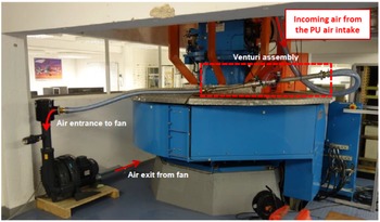
The aspiration is created with a fan placed at the ground floor and linked to the APU air intake with a plastic hose. A fan of type FPZ SCL K08-TD MOR IE2 has been used. This fan was chosen because it was immediately available for the campaign. The blower is able to create a maximal pressure delta of
 $ \pm $
425mbar corresponding to a volume flow of 518m
 $^3$
/h (equivalent in standard conditions of pressure and temperature to 178g/s). A typical rotational speed value of fan during the WTT is 2,250rpm (235.6Hz) to ensure a mass flow of 112g/s in standard atmospheric conditions. The maximal rotational speed of 2,940rpm has been used to synthetise the APU flow in approach, resulting in a massflow of 178g/s. The deviation of approx. 20g/s from the desired mass flow in approach has been considered as acceptable for the current purpose.
A Venturi assembly has been used to measure and monitor the mass flow created by the fan suction. An overview of the APU suction installation is proposed in Fig. 11. The complex suction system was shown to have a maximum of 2g/s of variations. Preliminary tests showed limited components at the fan frequency (and harmonics) in the spectral signature at the air intake on pressure and velocity.
2.6 Measurement means
2.6.1 Surface oil flow
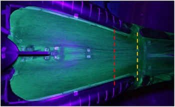
A specific liquid mixture has been used to be able to visualise the parietal flow topology in terms of friction lines on the surface of the rear cowlings. The liquid is mainly composed of kerosene, olive oil and UV pigments. The components are mixed to form a homogeneous liquid, which is applied on the upper cowlings. The wind speed is then put quickly to the nominal value of 40m/s. The kerosene drags the pigments along the friction lines and then evaporates. The result is a fixed and clear view of the friction lines when lighted by a UV lamp, as shown in Fig. 15. Separated areas appear in black, as the liquid cannot penetrate the separation boundaries. The wind needs to be set for roughly five minutes at nominal speed before the mix dries.
General view of the PU suction installation.

To facilitate result interpretation, equidistant lines are added on both sides of the rear cowlings. These lines are positioned along the longitudinal axis, with a 5cm distance between 2 lines, as depicted in Fig. 13. The first line is positioned at the aft of the pylon fairing.
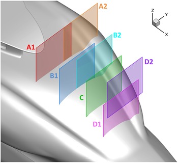
Overview of the seven PIV windows considered during the campaign, for zero angle-of-attack and zero yaw.

2.6.2 Particle Imagery Velocimetry (PIV)
A 2D-PIV measurement system has been used to measure the velocity components in the wake generated by the upper deck. The PIV measurement system is based on a laser plane delivered at a pulse frequency of 300Hz and a high-speed camera with a resolution of a
 $2,560 \times 1,600$
pixels, generating data at a rate of 3.4Gb/s. Seven PIV windows positioned perpendicularly to the fuselage centreline have been examined for each configuration and mock-up attitude, as illustrated in Fig. 12.
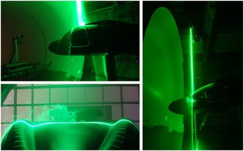
At the WT scale, plane family A is located 100mm downstream of the pylon-fairing trailing edge. The other plane families B, C and D are separated by 143mm along the longitudinal axis. In those areas, the instantaneous lateral and vertical velocity components are recorded. Roughly 1,500 snapshots (i.e. 5s of acquisition) have been needed to obtain converged mean-and-RMS velocity components with a tolerance of 1%. Given the distance between the camera and the laser plane, the effective field of view is of 316mm wide by 198mm high. Overviews of the PIV system are provided in Fig. 13.
2.6.3 Pressure probes at the cowling skin
Unsteady pressure measurements at the rear-cowling skin have been performed at locations as shown in Fig. 14. The pressure transducers are manufactured by Kulite, model XCQ-062, with a
 $ \pm $
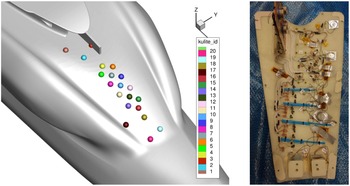
1psi range (differential pressure). Accuracy is roughly 0.1% of the full range, which gives an accuracy of 0.002psi or 13Pa. Unsteady pressures are recorded at a sampling frequency of 1,600Hz over a period of 30s. The complete pressure sensor implementation is depicted in Fig. 14. When mitigation means are implemented, overlapped sensors (e.g. sensor #3 in Fig.14) are deactivated.
General view of the PIV system during acquisition.

Left: pressure-sensor implementation on the rear cowlings and associated sensor ID. Right: Internal side of the rear cowling equipped with pressure sensors.

Left: Raw friction visualisation with surface oil flow. Right: Schematic flow-separation topology. Configuration AI_NONE
 $\textrm{AoA} = 0^{\circ}\;\textrm{AoY} = 0^{\circ}\;\textrm{U} = 40{\textrm{m/s}}$
.

Mean longitudinal vorticity in the PIV planes and interpreted vortex trajectory; configuration AI_NONE
 $\textrm{AoA} = 0^{\circ}\; \textrm{AoY} = 0^{\circ} \textrm{U} = 40{\textrm{m/s}}$
.

3.0 Results
3.1 Flow separation and wake topology over the baseline geometry
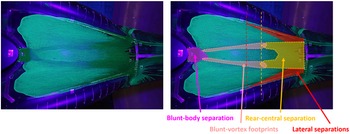
In this part, only the baseline configuration with no APU air intake is considered. It is aimed at providing a characterisation of the flow over the passive reference upper deck. Figure 15 shows the mean-flow separation topology at the rear cowlings for an angle-of-attack set to
 ${0^ \circ }$
(cruise conditions) and zero sideslip. Four different areas of flow separations are highlighted:
-
(i) A flow-separation zone at the pylon-fairing trailing edge (in magenta);
-
(ii) A central flow-separation area at the rear cowlings that goes up to about 30cm (6th line) upstream of the junction with the tail-boom, characterised by two long lateral branches (in yellow);
-
(iii) Two lateral flow-separation zones at the base of the longitudinal ridges on the rear-cowling sides (in red);
-
(iv) Two longitudinal separation lines characterised by a strong contraction of the friction lines, due to the two counter-rotating vortices generated at the pylon-fairing lips and convected in a close vicinity of the cowlings (in pink).
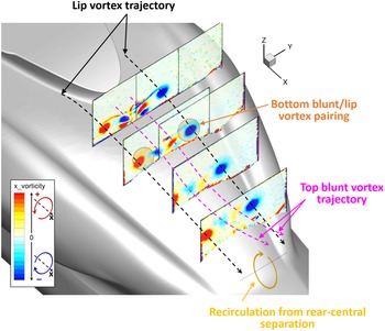
Figure 16 shows the mean longitudinal vorticity in the different PIV planes for a zero angle-of-attack and sideslip. The generation of two strong counter-rotating vortices at the pylon-fairing lips as described by Ref. (Reference Roesch and Vuillet5) is observed, along with the generation of a blunt-body wake at the base of pylon fairing following a pattern composed of four counter-rotating vortices. Lip vortices tend to remain rather close to the cowling skin. The rear-central flow separation at the aft cowlings highlighted by the surface oil flow leaves almost no traces on the mean longitudinal vorticity field, which tends to suggest that the wake generated in this area is more transversal. Intermediate PIV planes reveal that the blunt-body vortices tend to dissipate faster than the lip vortices. The bottom blunt vortices are co-rotating with the lip vortices and a vortex pairing can be observed in the PIV planes B. The field of mean longitudinal vorticity in the PIV plane D shows that the top blunt vortices generated by the rear of the pylon fairing – which remain rather close to the rear-cowling skin in PIV planes A – B and C are suddenly deviated in the vertical direction, likely because of a recirculation bubble generated by the rear-central flow separation at the aft cowlings. The global wake topology and vortex trajectories are sketched in Fig. 16.
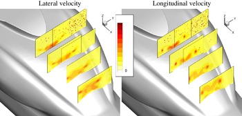
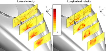
Unsteadiness in the flow may be assessed by computing the root mean square (RMS) velocity field along the lateral and vertical directions from all the PIV snapshots (Fig. 17). The lip vortices are shown to be very stable in PIV planes A, with only slight vertical oscillations of the vortex cores. The blunt-body wake generated at the rear of the pylon fairing shows much larger RMS levels. In planes B and C the vortex pairings described above between the lip vortices and the bottom blunt vortices appear clearly. Those interactions tend to significantly increase the lateral unsteadiness of the lip vortices, as it appears in plane D. The rear-central wake is mainly characterised by moderate levels of lateral RMS velocity.
RMS velocity field in the PIV planes. Left: Lateral velocity component. Right: Longitudinal velocity component. Configuration AI_NONE
 ${\textrm{AoA}} = 0^{\circ}\; {\textrm{AoY}} = 0^{\circ}\; \textrm{U} = 40{\rm{m/s}}$
.

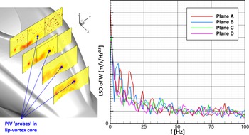
The spectral signature of the lip-vortex core fluctuations is analysed in Fig. 19. The Linear Spectral Density (LSD) – defined as the square root of the Power Spectral Density (PSD) – of the time signal of the vertical velocity is shown. The PSD have been computed using Hamming windowing and the periodogram overlapping technique with an overlap rate of 50%, resulting in a spectral resolution of 1Hz. Figure 18 reveals low-frequency fluctuations of lip-vortex cores all along their convection, in the range
 $[0;25]$
Hz. The secondary peaks around 5 and 15Hz observed in plane A are still present in plane B but tend to be damped in planes C and D, likely because of the vortex pairing with the bottom blunt vortices.
Left: RMS vertical velocity field in the PIV planes with probes located in the lip-vortex core. Right: Linear spectral density (LSD) of the vertical velocity component in the lip-vortex core in all PIV planes. Configuration AI_NONE
 ${\textrm{AoA}} = 0^{\circ}\; {\textrm{AoY}} = 0^{\circ}\; \textrm{U} = 40{\textrm{m/s}}$
.

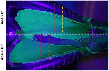
Locations of the mean flow-separation for
 ${\textrm{AoA}} = 0^{\circ}$
and
 ${\textrm{AoA}} = 10^{\circ}$
; rear-central separation in yellow; lateral separation in red. Configuration AI_NONE
 ${\textrm{AoY}} = 0^{\circ}\; \textrm{U} = 40{\textrm{m/s}}$
.

The mean-flow separation topology at the rear cowlings and the upper-deck wake pattern remain qualitatively rather the same for an angle-of-attack of
 ${10^ \circ }$
(approach conditions). The only major difference lies in the rear-central and lateral separation areas, which unsurprisingly extend upstream – by roughly additional 10cm – as well as the footprints of the lip vortices, which have been laterally spaced out, as shown in Fig. 19.
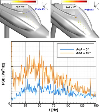
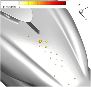
The signals recorded at the skin pressure sensors demonstrate low RMS pressure levels in both cases (
 ${\rm{AoA}}{ = 0^ \circ }$
and
 ${\rm{AoA}}{ = 10^ \circ }$
), except close to the base of pylon fairing where the RMS pressure notably increases, as illustrated in Fig. 20. In addition, those pressure fluctuations are characterised by a broadband spectral signature concentrated in the frequency range
 $[25;75]$
Hz.
Top: RMS pressure at the skin pressure sensors for
 ${\textrm{AoA}} = 0^{\circ}$
and
 ${\textrm{AoA}}= 10^{\circ}$
. The sensor sphere radii are sized and coloured by RMS pressure. Bottom: PSD of static pressure at probe #3. Configuration AI_NONE
 ${\rm{AoY}} = 0^{\circ}\; \textrm{U} = 40{\rm{m/s}}$
.

The risk of tail-shake associated with the baseline configuration is consequently believed to be small. The low-frequency components in the spectral signature of the pylon-fairing lips, along with a large separated areas at the rear cowlings are weak indicators of a potential risk of tail-shake. However, this is compensated by the moderate magnitudes of the unsteadiness in the upper-deck wake observed in the last PIV plane.
3.2 Influence of non-operating air intakes
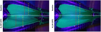
The influence of the APU air-intake positioning on the flow separation at the upper deck is highlighted in Fig. 21 in off mode, in cruise with a zero angle-of-attack and sideslip. The increase in the detached-flow area appears rather clearly when the air intake is located at the pylon-fairing trailing edge. A massive separation area appears along the centreline of the rear cowlings, extending upstream by 10 to 15cm with respect to the case without air intake. In addition, the lip-vortex footprints at the cowling skin are much more pronounced than in the case with no air intake. The impact of the AI_REF air intake is therefore negative in off mode, as its presence tends to be propitious to more wake generation. The second air intake (AI_BU) appears to have much less impact on the topology of the flow separation at the rear cowlings. Indeed, we observe separation areas that are quite comparable to what obtained without an air intake. The only slight difference is the larger flow separation area at the pylon-fairing trailing edge, as a result of the enlargement of the pylon fairing so as to allow the implementation of air ducts to collect fresh air at the pylon-fairing maximal cross-section.
Locations of the mean flow-separation for
 ${\textrm{AoA}} = 0^{\circ}$
; rear-central separation in yellow; lateral separation in red. Left: Configuration AI_REF. Right: Configuration AI_BU. Non-operating air intakes
 ${\textrm{AoY}} = 0^{\circ}\; \textrm{U} = 40{\rm{m/s}}$
.

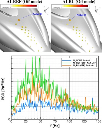
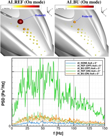
In terms of skin pressure, the largest RMS pressure are obtained at the base of pylon fairing. In off mode, both air intakes generate higher low-frequency components – in the range
 $[0:100]$
Hz – as it appears in Fig. 22. The increase is more important for the AI_REF configuration, originating from disturbances occurring in the inlet cavity.
Top: RMS pressure at the skin pressure sensors. Bottom: PSD of static pressure at probe #3. Non-operating air intakes
 ${\rm{AoA}} = 0^{\circ}\;{\textrm{AoY}} = 0^{\circ}\; \textrm{U} = 40{\rm{m/s}}$
.

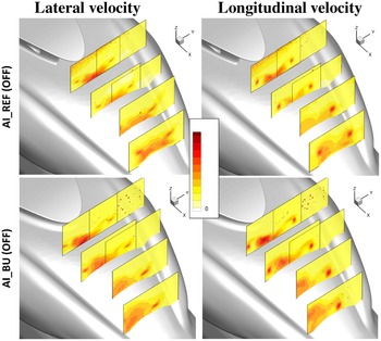
An overview of the RMS velocity fields is proposed in Fig. 23. An increase in the lateral turbulence intensity at the pylon-fairing trailing edge in the presence of the air intake AI_REF is highlighted. The air intake also seems to generate more lateral-velocity fluctuations along the whole central portion of the cowlings. In the last PIV plane, the topology of the flow observed without an intake (cf. Fig. 17) is modified when air intake AI_REF is implemented: a large zone of wake interactions is observed, regrouping the unsteadiness generated by the non-operating air intake, the wake arising from the rear-central flow detachment at the cowlings and the lip vortices. The lateral turbulence index may locally reach approx. 15%.
RMS velocity field in the PIV planes. Left: Lateral velocity component; Right: Longitudinal velocity component. Non-operating air intakes
 ${\textrm{AoA}} = 0^{\circ}\; {\textrm{AoY}} = 0^{\circ}\; \textrm{U} = 40{\rm{m/s}}$
.

Regarding the vertical RMS velocity field, the disturbance of the flow at the pylon-fairing trailing edge has little impact. The RMS lateral-and-vertical velocity fields obtained with the second air inlet AI_BU generally have slightly lower magnitudes than for the air intake at the pylon-fairing trailing edge. However, the fields are more asymmetric (a slight interaction between the left lip vortex and the blunt-body wake may be observed in planes B and D) and the areas of medium intensity – between 5% and 10% – are larger. A spectral analysis of lateral-and-vertical velocity fluctuations in the last PIV plane in areas maximising the RMS levels shows a frequency signature that is rather evenly distributed in frequency, with no clear peaks or broadband content. The spectral signature of the lip vortices remains roughly the same as in Fig. 18, but with slightly increased components in the low-frequency range
 $[0;25]$
Hz. The tail-shake risk induced by the non-operating air intakes increases to moderate for the two tested configurations. Indeed, the broadband spectral signature in the wake emission is still observed, with larger levels than for the baseline configuration without air intakes. For air intake #1, the cowlings are massively separated and the largest RMS values in skin pressure and velocity components in the volume are observed. For air intake #2 (AI_BU), the enlargement of the pylon fairing has been revealed to be penalising, as it produces a larger a more intense wake than with the thinner pylon fairing.
3.3 Influence of operating air intakes
During flight conditions for which additional power is required, the APU may operate and consequently, the air intake collects air to the power unit, creating a suction effect in its vicinity.
When the air intake operates, the flow-separation areas at the upper deck have only slightly increased compared to what is observed in off mode (cf. Fig. 21). However, the effect of the suction at the air intake is more significant on the skin-pressure fluctuations, especially for the air intake #1 (AI_REF), as illustrated in Fig. 24. It shows that the RMS levels are several times greater than what is observed when the air intake is inoperative and several dozen times greater than when the air intake is absent. The spectral content of pressure fluctuations at probe #3 is also shown. In the case of the operating air intake #1 (AI_REF), a broadband content in the range
 $[10;100]$
Hz is demonstrated. For operating air intake #2 (AI_BU), the levels are significantly lower, reaching the levels of the non-operating air intake #1. Its frequency signature remains rather broadband type, centred around
 $[25;75]$
Hz.
Top: RMS pressure at the skin pressure sensors. Bottom: PSD of static pressure at probe #3. Operating air intakes
 ${\textrm{AoY}} = 0^{\circ}\; \textrm{U} = 40{\rm{m/s}}$
.

An investigation of the pressure fluctuations at the cowlings around the nominal cruise conditions (zero angle-of-attack and sideslip) shows that the RMS levels tend to slightly increase as a function of the angle-of-attack (up to the tested value of
 ${12^ \circ }$
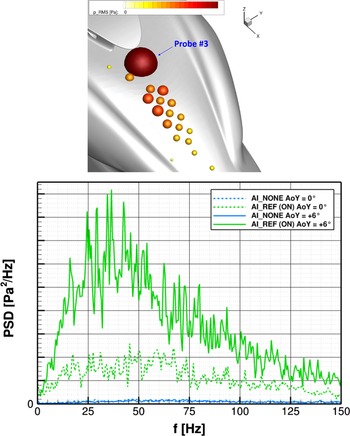
) for both air-intake designs. The low-frequency components of the spectral signature measured with at probe #3 tends to increase as well, especially for positive incidences. The effect is of course more pronounced for AI_REF. The impact of the yaw angle on the RMS pressure is impressive, particularly for the air intake located at the pylon-fairing trailing edge. Large to very large RMS levels are observed at almost all the pressure sensors, e.g. as shown in Fig. 25 for a yaw angle of
 $ + {6^ \circ }$
(i.e. wind from port side). At the probe located at the base of pylon fairing, the RMS level is very high, several times larger than what was observed for a zero yaw, for which high RMS levels have been already experienced. The broadband spectral signature is also preserved, with very high levels within the range
 $[25;75]$
Hz.
Top: RMS pressure at the skin pressure sensors for AI_REF configuration at
 ${\rm{AoY}} = + 6^{\circ}$
; the sensor sphere radii are sized and coloured by RMS pressure. Bottom: PSD of static pressure at probe #3. Operating air intakes;
 ${\rm{AoY}} = 6^{\circ}$
; PSD for a
 ${\rm{AoA}} = 0^{\circ}$
are also reported in dotted lines
 ${\rm{AoA}} = 0^{\circ}\; \textrm{U} = 40{\rm{m/s}}$
.

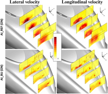
An overview of the RMS velocity field is proposed in Fig. 26 for both configurations. The air intake located at the pylon-fairing trailing edge is the source of a significant increase in the intensity of the lateral velocity fluctuations, with a large wake zone characterised by levels above typically 20% in the last PIV plane. A comparison to Fig. 23 reveals that the activation of the air intake AI_REF tends to dramatically increase spatially the size of the wake zones as well as the intensity of the fluctuations. Activating the second air intake (AI_BU) has a much more moderate effect on the lateral RMS velocity field, if not slightly beneficial. Indeed, the interactions between the left lip vortex and the blunt-body wake – observed when the air intake is inoperative – appears to be reduced. The vertical velocity field is also significantly impacted by the activation of the air intake #1 (AI_REF). Complex interactions are observed between the lip vortices, the wake of the air intake and the flow separations at the cowlings, which give rise to a vast wake zone characterised by very intense RMS levels, above 20% in the last plane of PIV. Air intake #2 behaves more transparently on the structure of the upper-deck wake. Indeed, a flow topology very comparable to what was observed for the baseline configuration (without air intake) is found. The overall level of fluctuations is, however, slightly higher at the base of the larger pylon fairing and in the core of the lip vortices because of the thicker aerofoil representing the pylon fairing.
RMS velocity field in the PIV planes. Left: Lateral velocity component; Right: Longitudinal velocity component. Operating air intakes
 ${\textrm{AoA}} = 0^{\circ}\; {\textrm{AoY}} = 0^{\circ}\; \textrm{U} = 40{\rm{m/s}}$
.

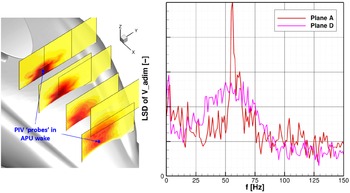
A spectral characterisation of the velocity fluctuations generated by air intake #1 (AI_REF) is proposed in Fig. 27. At the source (PIV plane A), evidence of strong lateral velocity fluctuations in the vicinity of the air intake is shown. The spectral signature exhibits significant levels up to 80Hz, with a dominant peak around 55Hz. This peak has been verified not to be correlated to the fan providing suction – which rotates at a frequency of 235Hz – nor any aliasing effects due the PIV bandlimit of 150Hz, which is smaller than the fan frequency. In the PIV plane D, the APU wake is characterised by a broadband spectral signature in the range
 $[25;90]$
Hz. Given the associated high magnitudes, a severe risk of potential tail-shake is anticipated.
Left: RMS lateral velocity field in the PIV planes with probes located in the APU wake. Right: Linear spectral density (LSD) of the lateral velocity component in APU wake. Configuration AI_REF; operating air intakes
 ${\textrm{AoA}} = 0^{\circ}\; {\textrm{AoY}} = 0^{\circ}\; \textrm{U} = 40{\rm{m/s}}$
.

3.4 Efficiency of mitigation means
In order to reduce the risk of tail-shake of the operating air intake #1 (AI_REF), two mitigations means have been proposed, based on patent EP3395690 [Reference Desvigne12]. The air intake AI_REF has been equipped with a separating wall mounted at the air-intake mouth along the cowling centreline (“dorsal fin”). The goal is to mitigate the intense lateral-velocity fluctuations appearing at the air-intake mouth, which – combined with their broadband spectral characteristics – constitute a potential severe source of tail-shake. The long dorsal fin did not show better results than the shorter one. Therefore, only the short variant of dorsal fins is at focus in the rest of the document. In what follows, the configuration AI_OA1_xe3 stands for the air intake AI_REF equipped with the short dorsal fin OA1_xe3.
The effect of the dorsal fin on the flow-separation pattern at the cowling skin is significant, as it appears in Fig. 28 for an angle-of-attack of
 ${\rm{AoA}}{ = 0^ \circ }$
. Indeed, the large areas of flow separation observed at the rear-centre cowling for the baseline configuration – and exacerbated by the operating air intake AI_REF – are completely eliminated. The trace of the lip vortices are also much attenuated. The lateral separations along the cowling ridges are drastically delayed as well.
Locations of the mean flow-separation for
 ${\textrm{AoA}} = 0^{\circ}$
. Rear-central separation in yellow; lateral separation in red. Configuration AI_AO1_xe3; operating air intakes
 ${\textrm{AoY}} = 0^{\circ}\; \textrm{U} = 40{\rm{m/s}}$
.

RMS pressure at the skin pressure sensors for AI_OA1_xe3 configuration. The sensor sphere radii are sized and coloured by RMS pressure. Operating air intakes
 ${\textrm{AoA}} = 0^{\circ}\; {\rm{AoY}} = 0^{\circ}\; U = 40{\rm{m/s}}$
.

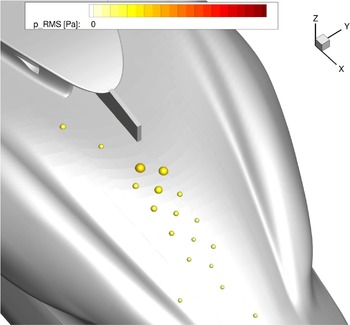
Along with the reduction of the flow-detachment areas, the levels of the RMS skin pressure have also notably decreased, as shown in Fig. 29, returning to levels comparable to what obtained when the APU is off (cf. Fig. 22).
RMS velocity field in the PIV planes. Left: Lateral velocity component. Right: Longitudinal velocity component. Configuration AI_OA1_xe3; operating air intakes
 ${\textrm{AoA}} = 0^{\circ}\; {\textrm{AoY}} = 0^{\circ }\; \textrm{U} = 40{\rm{m/s}}$
.

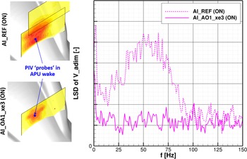
Left: RMS lateral velocity field in the PIV plane D with probes located at the maximum RMS level. Right: Linear spectral density (LSD) of the lateral velocity component in APU wake. Operating air intakes
 ${\rm{AoA}} = 0^{\circ}\; {\textrm{AoY}} = 0^{\circ}\; \textrm{U} = 40{\rm{m/s}}$
.

RMS pressure at the skin pressure sensors for AI_OA1_xe3 configuration. The sensor sphere radii are sized and coloured by RMS pressure
 ${\rm{AoA}} = 0^{\circ}\; {\textrm{AoY}} = + 6^{\circ}\; \textrm{U} = 40{\rm{m/s}}$
.

Figure 30 shows the influence of dorsal fin on lateral-and-vertical RMS velocity in the different PIV planes. The effect of the dorsal fin on the wake mitigation is spectacular; indeed a reduction of more than 50% in the RMS lateral velocity is observed in the last PIV plane, which was the expected effect. More precisely, the wake at the air-intake mouth has been revealed to be almost fullly suppressed, and the wake observed in PIV plane D is principally the wake of the dorsal fin itself. In addition, the dorsal fin is shown to also play a beneficial role in mitigating the velocity fluctuations in the vertical direction.
In terms of spectral components contained in the wake, the broadband characteristics of the wake generated by the air intake are perfectly mitigated by the dorsal fin, as illustrated in Fig. 31, which shows the spectral decomposition of the lateral-velocity fluctuations at a location in plane D which maximise the associated RMS level.
The robustness of the benefits from the dorsal fin has been investigated for angle-of-attack up to
 $ + {10^ \circ }$
and a yaw angle up to
 $ + {6^ \circ }$
. The flow is reportedly kept well attached along the cowlings, except in the vicinity of the tail-boom junction where the rear-central separation slightly increases. The case of yaw of
 $ + {6^ \circ }$
was particularly interesting because it maximised the RMS levels of skin pressure on the cowlings when the air intake AI_REF operated. The critical situation has also been well mitigated by the dorsal fin, as shown in Fig. 32.
When the APU does not operate, the dorsal fin has almost no effect on the wake generated at the upper deck.
4.0 Conclusions
A wind-tunnel test campaign aimed at assessing the role of the upper-deck – including two different air-intake designs installed on it – as a potential source of tail-shake has been performed at Airbus Helicopters’ Marignane wind-tunnel facilities. The campaign has been conducted on a mock-up representative of the upper deck of a heavy-weight class helicopter, in the form of a minibody model. A scale 1:3.5 has been considered so as to preserve the representativeness of the flow over the H/C upper deck. Given the large size of the model, the tail-shake risks have been characterised at the source only. The campaign mostly focuses on flight conditions around cruise and approach, for which the typical tail-shake frequency range could be rescaled respectively to
 $[9;37]$
and
 $[17;70]$
Hz at the WT scale.
Different measurement methods to evaluate aerodynamic interactions and wake sources are proposed. They consist in flow-separation assessments from skin-friction painting visualisations, time-resolved particle image velocimetry (PIV) measurements in the volume, as well as unsteady pressure measurements at the cowlings. Basically, a configuration that produces strong vortices characterised by a broadband spectral signature is believed to gather all the conditions for tail-shake to emerge. Based on the analysis carried out in this document, the following major conclusions are drawn:
-
(i) For all the angle-of-attack and sideslip combinations studied, the flow-separation topology is characterised by four distinct zones for the baseline configuration (i.e. without air intakes), the most critical ones being the blunt-body separation at the pylon-fairing trailing edge and a large flow-separation area appearing at the rear-central part of the cowlings. The analysis based on the PIV measurements of the lateral-and-vertical velocity components indicates a wake pattern composed of well-established lip vortices which are then slightly disturbed by the wake generated by the rear of the pylon fairing. The resulting low-frequency spectral components in the upper-deck wake, along with rather low RMS levels indicate a small risk of tail-shake for the baseline configuration.
-
(ii) The presence of an inoperative air intake at the rear of the pylon fairing (air intake #1) causes a significant increase in the flow-detachment area at the aft cowlings, associated with higher skin-pressure RMS levels, especially in the vicinity of the air intake. In the volume, the wake pattern described for the baseline configuration has been fairly modified: a large area of intense wake interaction is observed, regrouping the disturbances generated by the non-operating air intake, the wake originating from the flow separation at rear-central cowlings and the lip vortices generated by the pylon fairing curved sides, in total interaction. The lateral turbulence index locally reaches approx. 15%. The risk of tail-shake is higher accordingly.
-
(iii) The operating air intake #1 has a strong effect on the flow unsteadiness. Large to very large RMS levels are observed at almost all the skin-pressure sensors. The upper-deck wake is characterised by very strong lateral-velocity RMS levels, along with a broadband spectral signature in the range
$[25;90]$
Hz. Therefore the risk of tail-shake is believed to be high in this case. -
(iv) A mitigation mean has been investigated in the form of a separating wall (or “dorsal fin”) mounted at the mouth of the air intake, so as to reduce the lateral velocity fluctuations at its vicinity. The benefits on the wake mitigation is spectacular: a reduction of more than 50‘% on the RMS levels of both lateral-and-vertical velocity components are observed, along with the total suppression of the broadband component in the wake spectral signature. The robustness of the benefits with small variations of angle-of-attack and sideslip has also been verified.
-
(v) A second air-intake design has been evaluated. It consists in two air intakes implemented on each side of the pylon fairing, close to its maximum cross-section location. An enlargement of the pylon fairing by 100mm (at scale 1:1) on each side has been required to implement the ducts from the inlets to the APU. This type of implementation is more classical but it has several drawbacks, in particular the increase of the H/C empty weight due to the ducts and the larger pylon fairing, along with less efficient air intakes in hover. This air-intake concept appears to be less intrusive on the flow structure at the upper deck. However, the enlargement of the pylon fairing exacerbates the blunt-body separation at the pylon-fairing trailing edge. The flow analysis demonstrates that this concept does not provide significantly better results regarding the tail-shake risk than the air intake implemented at the pylon-fairing trailing edge with the dorsal fin despite notable penalties on weight and hover performance.

Acknowledgements
This work was supported by CHAllenge AéRo-thermo-MEchanique (CHARME) Projects, partially funded by Direction Générale de l’Aviation Civile (DGAC). The authors are grateful for the support from Debbie Leusink and Manuel Bucharles.