1 Introduction
Turbulence at a high Reynolds number consists of innumerable vortices with various scales. Although the characteristics of large-scale vortices depend on the driving force and/or the boundary conditions of the flow, the statistics of smaller-scale vortices are independent of them. This small-scale universality was predicted by the similarity hypothesis of Kolmogorov (Reference Kolmogorov1941) and it has been supported by many experiments and direct numerical simulations (DNS) of statistically stationary turbulence. The similarity hypothesis therefore gives the basis for the theories of turbulence. In textbooks on turbulence (Tennekes & Lumley Reference Tennekes and Lumley1972; Frisch Reference Frisch1995; Davidson Reference Davidson2004), the origin of the hypothesis is explained in terms of the energy cascade. Namely, through the scale-by-scale energy transfer from larger to smaller vortices, small-scale vortices become independent of the characteristics of the large-scale vortices.
Although the energy cascade is essential in the dynamics of turbulence, its physical mechanism is not fully understood. This is because we need to investigate the dynamics of three-dimensional structures in turbulence at high Reynolds numbers with a sufficiently large scale separation. For the turbulence in a periodic cube, which is a model of turbulence away from solid walls, many authors (Kerr Reference Kerr1985; Hussain Reference Hussain1986; Melander & Hussain Reference Melander and Hussain1993; Goto Reference Goto2008, Reference Goto2012; Cardesa, Vela-Martin & Jiménez Reference Cardesa, Vela-Martin and Jiménez2017; Goto, Saito & Kawahara Reference Goto, Saito and Kawahara2017) investigated the physical mechanism of the energy cascade. In a periodic cube, smaller-scale turbulent vortices are created by vortex stretching in larger-scale strain-rate fields. However, in a periodic cube, we need an external body force to sustain the hierarchy of vortices. On the other hand, in a more realistic situation, where an external body force is absent (or rotation-free), it is a solid wall that generates vorticity. The main aim of the present study is to reveal the sustaining mechanism of a hierarchy of multiscale vortices in a fully developed zero-pressure-gradient turbulent boundary layer over a flat plate, which is the most fundamental turbulent flow near a wall.
Although DNS of the wall-bounded turbulence have revealed quite a few pieces of important knowledge of its dynamics and statistics (see the review by Jiménez (Reference Jiménez2018) and references therein), there are only a few studies that focus on the small-scale universality. Jiménez (Reference Jiménez2012) reviewed studies at that time on the self-similarity of the flow structures and cascades in wall-bounded turbulence. Recently, Cimarelli et al. (Reference Cimarelli, De Angelis, Jiménez and Casciola2016) examined energy cascade in turbulent channel flows to show that the anisotropic production and inhomogeneous flux lead to complex dynamics of the cascades. We emphasize that current supercomputers are powerful enough to investigate the physics behind the small-scale universality of the wall-bounded turbulence. In fact, the DNS (e.g. Schlatter et al. Reference Schlatter, Li, Örlü, Hussain and Henningson2014), as well as the experiments (e.g. Hutchins & Marusic Reference Hutchins and Marusic2007), of high-Reynolds-number turbulent boundary layers show the so-called second peak (see figure 2 c, below) of the premultiplied spanwise energy spectrum. As will be discussed below (see § 2.1), the appearance of the second peak is evidence of the scale separation, because it is associated with the existence of large-scale structures (Tomkins & Adrian Reference Tomkins and Adrian2003; Hambleton, Hutchins & Marusic Reference Hambleton, Hutchins and Marusic2006; Hutchins & Marusic Reference Hutchins and Marusic2007; Dennis & Nickels Reference Dennis and Nickels2011b ; Schlatter et al. Reference Schlatter, Li, Örlü, Hussain and Henningson2014; Lee, Sung & Zaki Reference Lee, Sung and Zaki2017). Incidentally, the second peak was observed not only in turbulent boundary layers but also in turbulence in a pipe (Kim & Adrian Reference Kim and Adrian1999) and in a channel (Abe, Kawamura & Choi Reference Abe, Kawamura and Choi2004; Toh & Itano Reference Toh and Itano2005; Hwang Reference Hwang2015). Some of the studies demonstrated that it is associated with large-scale counter-rotating roll modes (del Álamo et al. Reference del Álamo, Jiménez, Zandonade and Moser2006; Marusic & Hutchins Reference Marusic and Hutchins2008; Hutchins et al. Reference Hutchins, Chauhan, Marusic, Monty and Klewicki2012). We therefore conduct DNS of a turbulent boundary layer with the second peak of the premultiplied spanwise energy spectrum to investigate the generation mechanism of multiscale vortices in the turbulence. Though the Reynolds number examined in the present study is not higher than the recent DNS by other authors (e.g. Borrell, Sillero & Jiménez Reference Borrell, Sillero and Jiménez2013; Schlatter et al. Reference Schlatter, Li, Örlü, Hussain and Henningson2014), we use a simple coarse-graining method and detailed statistical analysis to reveal the multiscale nature of turbulent boundary layers.
The scope of the present study is in revealing the real-space image and sustaining mechanism of the hierarchical structure of multiscale vortices in a high-Reynolds-number turbulent boundary layer. These lay the foundation for future studies on the energy cascade and small-scale universality of wall-bounded turbulence. More concretely, in the present paper, we propose the scenario of the generation mechanism of the hierarchy of vortices in a high-Reynolds-number turbulent boundary layer. (i) In the log layer of high-Reynolds-number turbulent boundary layers, large- and small-scale vortices coexist. Large-scale vortices with the size of the order of the distance from the wall are stretched and amplified by the mean flow, whereas smaller-scale vortices are generated predominantly by stretching in strain-rate fields induced by the large-scale vortices. In other words, small-scale vortices are created by an energy cascade process. (ii) In the buffer layer, in contrast, since there is no scale separation, vortices are stretched directly by the mean flow. (iii) Similarly, in low-Reynolds-number turbulent boundary layers, there are only vortices with the size of the order of the boundary layer thickness, and they are stretched and amplified directly by the mean shear. The crossover of the dominance of the stretching from mean flow to larger-scale vortices occurs at a Reynolds number at which the energy spectrum shows the inertial-range scaling.
In the rest of the present paper, we quantitatively verify the proposed scenario of the generation mechanism of the hierarchy of vortices. For this purpose, we identify the hierarchy of multiscale vortices by applying a Gaussian filter to the DNS velocity field. Numerical schemes of the DNS and the coarse-graining method are described in § 2. By analysing the coarse-grained velocity field, we numerically examine, in § 3, how vortices at a given scale are created. These statistical analyses allow us to verify the proposed scenario. Furthermore, we demonstrate, in § 4, concrete examples of the generation process of the hierarchy of vortices in the log layer, which also support the scenario.
2 Numerical methods
2.1 Direct numerical simulation
We numerically simulate a zero-pressure-gradient turbulent boundary layer over a flat plate by solving the Navier–Stokes equations of an incompressible fluid by a standard finite difference scheme. The streamwise, wall-normal and spanwise directions are denoted by
 $x$
,
 $y$
and
 $z$
, and the velocity components in these directions are by
 $u$
,
 $v$
and
 $w$
, respectively. The terms in the governing equations are spatially discretized by using a fully conservative second-order central difference scheme on a staggered grid (Kajishima & Taira Reference Kajishima and Taira2017, pp. 73–146). A non-uniform grid is set in the wall-normal direction so that small-scale structures in the near-wall region are well resolved (the grid width in the wall-normal direction is always finer than
 $1.5\unicode[STIX]{x1D702}$
in terms of the Kolmogorov length
 $\unicode[STIX]{x1D702}$
). The viscous terms are integrated in time implicitly by using the second-order Crank–Nicolson method and the convective terms are treated explicitly by using the second-order Adams–Bashforth method. Applying the simplified marker and cell (SMAC) method (Amsden & Harlow Reference Amsden and Harlow1970) to the governing equations, we solve the four-step time-advancement equations.
Since the difficulty of the DNS of high-Reynolds-number turbulent boundary layers stems from the inflow turbulence generation, several techniques have been proposed (see the review by Wu (Reference Wu2017) for methods about how to impose an inlet condition). In the present study, we use the time-series data of the fully developed turbulent velocity field at
 $Re_{\unicode[STIX]{x1D703}}=U_{\infty }\unicode[STIX]{x1D703}/\unicode[STIX]{x1D708}=1200$
(
 $Re_{\unicode[STIX]{x1D70F}}=u_{\unicode[STIX]{x1D70F}}\unicode[STIX]{x1D6FF}_{99}/\unicode[STIX]{x1D708}=452$
) provided by Lee et al. (Reference Lee, Jung, Sung and Zaki2013, Reference Lee, Sung and Zaki2017) for the inflow condition, where
 $U_{\infty }$
is the free-stream velocity,
 $\unicode[STIX]{x1D703}$
is the momentum thickness,
 $\unicode[STIX]{x1D708}$
is the kinematic viscosity, and
 $u_{\unicode[STIX]{x1D70F}}$
is the skin-friction velocity. For the top boundary conditions (
 $y=L_{y}$
), we impose
 $\unicode[STIX]{x2202}u/\unicode[STIX]{x2202}y=\unicode[STIX]{x2202}w/\unicode[STIX]{x2202}y=0$
and the suction velocity
 $v$
, which is determined (in the same way as in Lee et al. (Reference Lee, Sung and Zaki2017)) by the experimental data (Monkewitz, Chauhan & Nagib Reference Monkewitz, Chauhan and Nagib2008), to maintain a zero streamwise pressure gradient on average. The non-slip boundary condition is imposed at the wall (
 $y=0$
). The boundary condition at the exit (
 $x=L_{x}$
) of the computational domain is
 $\unicode[STIX]{x2202}u_{i}/\unicode[STIX]{x2202}t+U_{c}\unicode[STIX]{x2202}u_{i}/\unicode[STIX]{x2202}x=0$
, where
 $U_{c}$
is the bulk velocity at the exit, with a small correction to enforce the global mass conservation (see Simens et al.
Reference Simens, Jiménez, Hoyas and Mizuno2009). The periodic boundary condition is imposed in the spanwise direction.
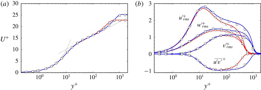
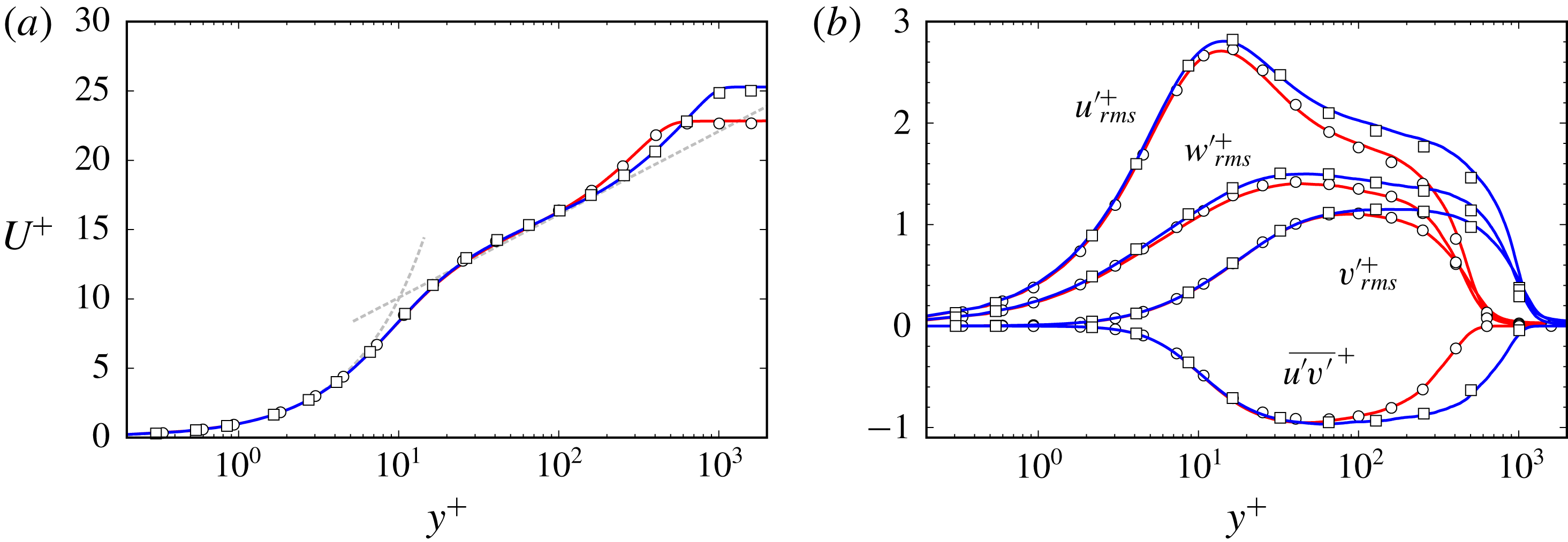
Wall-normal profiles of (a) the mean streamwise velocity and (b) the root-mean-square values of the fluctuation velocity components and the turbulent stress. Red line, the present DNS at
 $Re_{\unicode[STIX]{x1D703}}=1410$
; blue line, the present DNS at
 $Re_{\unicode[STIX]{x1D703}}=3030$
; open circles, Schlatter & Örlü (Reference Schlatter and Örlü2010) at
 $Re_{\unicode[STIX]{x1D703}}=1410$
; open squares, Schlatter & Örlü (Reference Schlatter and Örlü2010) at
 $Re_{\unicode[STIX]{x1D703}}=3030$
. In (a) the grey dashed lines indicate the law of the wall:
 $U^{+}=y^{+}$
and
 $U^{+}=(1/\unicode[STIX]{x1D705})\ln (y^{+})+B$
, with
 $\unicode[STIX]{x1D705}=0.384$
and
 $B=4.1$
.
Numerical parameters of the DNS. Here,
 $L_{x},~L_{y}$
and
 $L_{z}$
are the sides of the computational domain (where
 $\unicode[STIX]{x1D703}_{in}$
is the momentum thickness at the inlet),
 $N_{x},~N_{y}$
and
 $N_{z}$
are the numbers of grid points, and
 $\unicode[STIX]{x0394}x^{+},\unicode[STIX]{x0394}y_{min}^{+}$
and
 $\unicode[STIX]{x0394}z^{+}$
are the resolutions at the downstream exit.

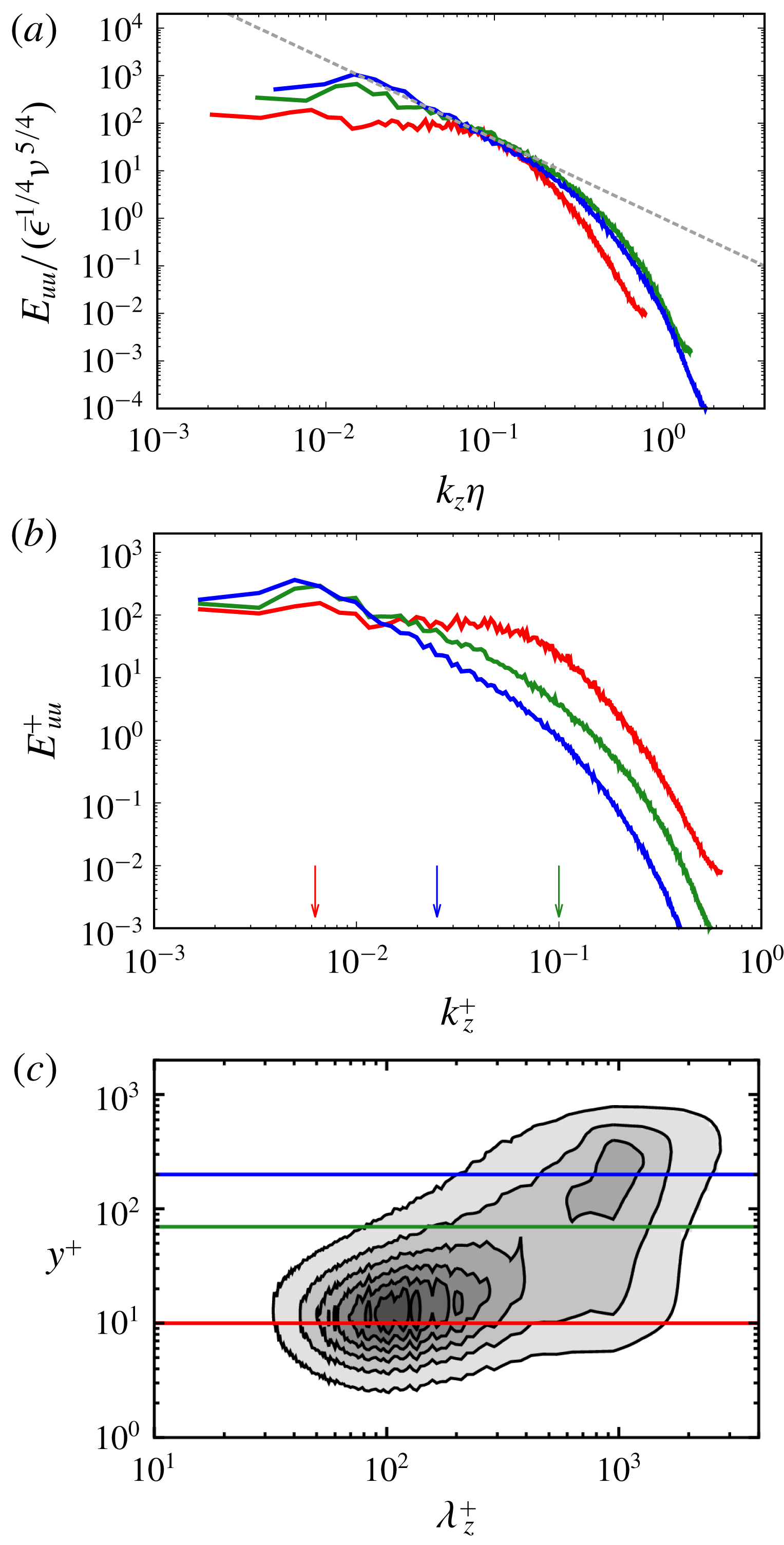
(a) Spanwise energy spectrum
 $E_{uu}^{+}$
(non-dimensionalized by the mean energy dissipation rate
 $\overline{\unicode[STIX]{x1D716}}$
and by
 $\unicode[STIX]{x1D708}$
) of the streamwise velocity component at three heights,
 $y^{+}=10$
(red),
 $70$
(green) and
 $200$
(blue), at a streamwise location corresponding to
 $Re_{\unicode[STIX]{x1D703}}=3170$
. The grey dashed line indicates the
 $-5/3$
power law,
 $E_{uu}\propto k_{z}^{-5/3}$
. (b) The same as in (a) but in wall units. The arrows indicate the spanwise wavenumber (
 $k_{z}^{+}=1/\unicode[STIX]{x1D70E}^{+}$
) corresponding to the three filter scales in figure 4. (c) Premultiplied spanwise energy spectrum
 $k_{z}^{+}E_{uu}^{+}$
of the streamwise velocity component at
 $Re_{\unicode[STIX]{x1D703}}=3170$
as a function of the height
 $y^{+}$
and the spanwise wavelength
 $\unicode[STIX]{x1D706}_{z}^{+}$
. The coloured lines indicate the heights for which
 $E_{uu}$
is shown in (a) and (b).
The numerical parameters of this DNS are given in table 1. The domain size is the same as the DNS of Lee et al. (Reference Lee, Sung and Zaki2017) and the number of grid points is also almost the same. To validate this simulation, figure 1 shows the wall-normal profiles of the mean streamwise velocity
 $U$
and root-mean-square values
 $u_{rms}^{\prime }$
,
 $v_{rms}^{\prime }$
and
 $w_{rms}^{\prime }$
of the velocity components and the turbulent stress
 $\overline{u^{\prime }v^{\prime }}$
at two different Reynolds numbers, which are in good agreement with the results of Schlatter & Örlü (Reference Schlatter and Örlü2010) as well as Lee et al. (Reference Lee, Sung and Zaki2017). Here, the superscript plus sign
 $\cdot ^{+}$
denotes the wall units defined in terms of
 $u_{\unicode[STIX]{x1D70F}}$
and
 $\unicode[STIX]{x1D708}$
; and the overbar
 $\overline{\,\cdot \,}$
denotes the average in the spanwise direction and time.
Before verifying the scenario of the sustaining mechanism of a hierarchy of multiscale vortices, it is important to show that the simulated turbulence is fully developed to have a hierarchy. Figure 2(a) shows the spanwise energy spectrum
 $E_{uu}(k_{z})$
(non-dimensionalized by the mean energy dissipation rate
 $\overline{\unicode[STIX]{x1D716}}$
and by
 $\unicode[STIX]{x1D708}$
) of the streamwise velocity component at the three heights (
 $y^{+}=10$
,
 $70$
and
 $200$
) for the Reynolds number
 $Re_{\unicode[STIX]{x1D703}}=3170$
(
 $x=980\unicode[STIX]{x1D703}_{in}$
). We can see that the turbulence at
 $y^{+}=200$
has a broad energy spectrum, which approximately obeys the
 $-5/3$
power law. We therefore expect that the turbulence is composed of a hierarchy of multiscale vortices. The scaling range disappears in the near-wall region.
We also plot the premultiplied energy spectrum
 $k_{z}^{+}E_{uu}^{+}$
as a function of the wavelength
 $\unicode[STIX]{x1D706}_{z}^{+}$
and the height
 $y^{+}$
in figure 2(c). We observe not only the first peak at
 $y^{+}\approx 10$
and
 $\unicode[STIX]{x1D706}_{z}^{+}\approx 10^{2}$
but also the second one at
 $y^{+}\approx 10^{2}$
and
 $\unicode[STIX]{x1D706}_{z}^{+}\approx 10^{3}$
. It is often explained that the former peak indicates the near-wall streak structure and the latter large-scale motion. It is evident in figure 2 that when the
 $-5/3$
power law of
 $E_{uu}$
is established (the blue curves in figure 2
a,b), the second peak of the premultiplied energy spectrum also appears (figure 2
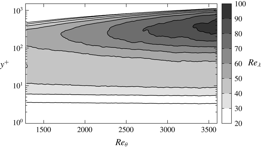
c). As will be shown below (see figure 9 in § 3.2), the Taylor-length-based Reynolds number
 $Re_{\unicode[STIX]{x1D706}}$
is approximately
 $90$
at
 $y^{+}=300$
and
 $Re_{\unicode[STIX]{x1D703}}=3170$
, where the second peak is observed. This is consistent with the appearance of the inertial range, which requires
 $Re_{\unicode[STIX]{x1D706}}\gtrsim 50$
. We will show in the following that the generation mechanisms of vortices are essentially different in low- and high-Reynolds-number turbulent boundary layers. Here, high-Reynolds-number turbulence denotes the flow with a hierarchy of vortices in real space and with the statistics such as the
 $-5/3$
power law of
 $E_{uu}$
and the second peak of
 $k_{z}E_{uu}$
.
2.2 Coarse-graining method
Several methods have been proposed to identify the hierarchy of vortices at different scales. For example, a band-pass filter (Leung, Swaminathan & Davidson Reference Leung, Swaminathan and Davidson2012; Goto et al. Reference Goto, Saito and Kawahara2017) or a low-pass filter (Goto Reference Goto2008, Reference Goto2012) of the Fourier modes were used for turbulence in a periodic cube. However, we cannot educe the structures at an arbitrary scale using these methods in a turbulent boundary layer, since the flow is inhomogeneous in the streamwise and wall-normal directions. For turbulent boundary layers, to separate the near-wall streak structures from the larger-scale flow, Tomkins & Adrian (Reference Tomkins and Adrian2003) used low-pass filtering only in the spanwise direction. Lee & Sung (Reference Lee and Sung2011) and Lee et al. (Reference Lee, Sung and Zaki2017) applied Gaussian filters to the velocity to highlight large-scale motions in turbulent boundary layers, and many other authors (Lee et al. Reference Lee, Lee, Choi and Sung2014; Hwang et al. Reference Hwang, Lee, Sung and Zaki2016; Lozano-Durán, Holzner & Jiménez Reference Lozano-Durán, Holzner and Jiménez2016, e.g.) used Gaussian filters to identify arbitrary-scale motions in turbulent channel flows. Incidentally, del Álamo et al. (Reference del Álamo, Jiménez, Zandonade and Moser2006) extracted large-scale vortical structures by conditionally averaging velocity fields.
In this study, we also identify quantities at a given scale by applying the three-dimensional Gaussian filter to the velocity field,
 $$\begin{eqnarray}\displaystyle \tilde{u} _{i}(x,y,z;\unicode[STIX]{x1D70E}) & = & \displaystyle \mathop{\sum }_{z_{p}}\mathop{\sum }_{y_{p}}\mathop{\sum }_{x_{p}}u_{i}(x_{p},y_{p},z_{p})\nonumber\\ \displaystyle & & \displaystyle \times \underbrace{C(y)\exp \left(-\frac{2}{\unicode[STIX]{x1D70E}^{2}}((x_{p}-x)^{2}+(y_{p}-y)^{2}+(z_{p}-z)^{2})\right)\unicode[STIX]{x0394}x\unicode[STIX]{x0394}y\unicode[STIX]{x0394}z}_{K(x_{p},y_{p},z_{p};x,y,z)}.\nonumber\\ \displaystyle & & \displaystyle\end{eqnarray}$$
Here,
 $x_{p}$
,
 $y_{p}$
and
 $z_{p}$
are located at grid points, and
 $C$
is a coefficient to ensure that the summation of the Gaussian kernel,
 $K$
, is unity, i.e.
 $$\begin{eqnarray}\mathop{\sum }_{z_{p}}\mathop{\sum }_{y_{p}}\mathop{\sum }_{x_{p}}K(x_{p},y_{p},z_{p};x,y,z)=1.\end{eqnarray}$$
Note that the filter scale
 $\unicode[STIX]{x1D70E}$
is twice as large as that defined in Lee et al. (Reference Lee, Sung and Zaki2017). The Gaussian filter corresponds to the low-pass filter of the Fourier mode, and the coarse-grained velocity
 $\tilde{u} _{i}$
defined by (2.1) contains the information larger than
 $\unicode[STIX]{x1D70E}$
. We evaluate the coarse-grained quantity
 $q^{(\unicode[STIX]{x1D70E})}$
from the coarse-grained velocity
 $\tilde{u} _{i}$
.
3 Results
3.1 Hierarchy of vortices
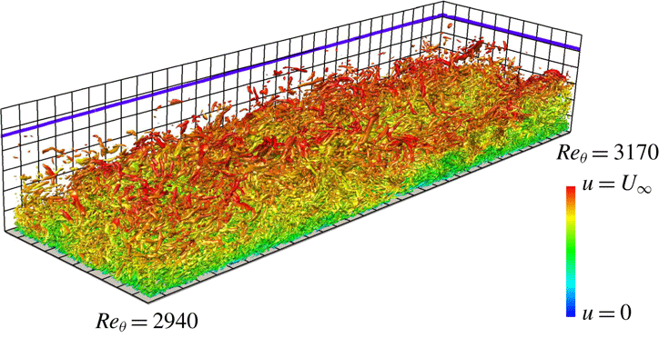
Isosurfaces of the second invariant
 $Q^{+}~(=1.6\times 10^{-3})$
of the velocity gradient tensor. The threshold is set as
 $m_{Q}+0.4s_{Q}$
. The colour indicates the streamwise velocity
 $u$
, ranging from
 $u=0$
(blue) to
 $u=U_{\infty }$
(red). Half of the spanwise direction of the computational domain is visualized. The Reynolds number
 $Re_{\unicode[STIX]{x1D703}}$
changes from
 $2940$
to
 $3170$
in the streamwise direction. The flow is from lower left to upper right. The black grid width is
 $200$
wall units evaluated at the plane corresponding to
 $Re_{\unicode[STIX]{x1D703}}=2860$
, and the blue solid line indicates the
 $99\,\%$
boundary layer thickness
 $\unicode[STIX]{x1D6FF}_{99}$
.

To capture vortical structures in turbulent shear flows, the second invariant
 $Q~(=1/2\unicode[STIX]{x1D6FA}_{ij}\unicode[STIX]{x1D6FA}_{ij}-1/2\unicode[STIX]{x1D61A}_{ij}\unicode[STIX]{x1D61A}_{ij})$
of the velocity gradient tensor is widely used, where
 $\unicode[STIX]{x1D6FA}_{ij}$
and
 $\unicode[STIX]{x1D61A}_{ij}$
are the rate-of-rotation and rate-of-strain tensors. Setting the criterion as
 $Q>Q_{0}$
, with
 $Q_{0}$
being a positive threshold, we can identify vortical regions. Let us start by observing vortical structures identified by the
 $Q$
criterion without the coarse-graining. Previous DNS of turbulent boundary layers at high Reynolds numbers showed that hairpin vortices disappear in downstream regions (Jiménez et al.
Reference Jiménez, Hoyas, Simens and Mizuno2010; Schlatter et al.
Reference Schlatter, Li, Örlü, Hussain and Henningson2014). Our DNS also shows similar results. Figure 3 illustrates the vortical structures obtained by our DNS with a choice of
 $Q_{0}=m_{Q}+0.4s_{Q}$
, so that those in the log layer are visualized. Here,
 $m_{Q}$
and
 $s_{Q}$
are, respectively, the mean and standard deviation of
 $Q$
at
 $y^{+}=200$
and
 $Re_{\unicode[STIX]{x1D703}}=3170$
. Some of the vortices visualized in the region apart from the wall are arch-like, but they are not connected to streamwise vortices. Schlatter et al. (Reference Schlatter, Li, Örlü, Hussain and Henningson2014) also showed similar results by using the
 $\unicode[STIX]{x1D706}_{2}$
criterion (Jeong & Hussain Reference Jeong and Hussain1995). Here,
 $\unicode[STIX]{x1D706}_{2}$
is the second eigenvalue of
 $\unicode[STIX]{x1D61A}_{ik}\unicode[STIX]{x1D61A}_{kj}+\unicode[STIX]{x1D6FA}_{ik}\unicode[STIX]{x1D6FA}_{kj}$
. These DNS results imply that it is hard to identify hairpin vortices by using the
 $Q$
or
 $\unicode[STIX]{x1D706}_{2}$
criteria in a turbulent boundary layer at high Reynolds numbers. We must, however, emphasize that the velocity gradient tensor, and therefore
 $\unicode[STIX]{x1D6FA}_{ij}$
,
 $\unicode[STIX]{x1D61A}_{ij}$
,
 $Q$
and
 $\unicode[STIX]{x1D706}_{2}$
, are associated with the smallest-scale vortices. Therefore, the
 $Q$
or
 $\unicode[STIX]{x1D706}_{2}$
criterion identifies only the smallest-scale vortices. Multiscale vortices ranging from the length of the order of the boundary layer thickness to the Kolmogorov length coexist in the turbulence at high Reynolds numbers. Therefore, until we identify each scale of the vortices, we cannot approach the intrinsic vortex dynamics in a turbulent boundary layer.
Next, to identify such multiscale coherent structures, and to quantitatively verify the scenario proposed in § 1, we apply the Gaussian filter (2.1) to the velocity field. We show the isosurfaces of the second invariant
 $Q^{(\unicode[STIX]{x1D70E})}$
of the velocity gradient tensor coarse-grained at three length scales in figure 4, to see if a hierarchy of vortices can be captured by this coarse-graining method. The three filter scales are set as
 $\unicode[STIX]{x1D70E}^{\oplus }=10$
(figure 4
a),
 $40$
(figure 4
b) and
 $160$
(figure 4
c), where
 $\cdot ^{\oplus }$
denotes non-dimensionalization in wall units at
 $Re_{\unicode[STIX]{x1D703}}=2860$
. The arrows in figure 2(b) indicate the spanwise wavenumbers corresponding to these filter scales. We choose the thresholds of the isosurfaces as
 $Q_{0}=m_{Q}+0.5s_{Q}$
so that the vortices in the log layer are visualized. Figure 4 shows that a hierarchy of vortices indeed exists in the turbulent boundary layer. Noting that
 $200$
wall units are indicated by the grid width, we may see that the length scales of the vortices approximately correspond to the filter scales. In particular, we notice that at
 $\unicode[STIX]{x1D70E}^{\oplus }=160$
(figure 4
c) the larger-scale vortices have spatially organized structures and some of them are arch-like (see § 4.1 for more detailed discussions). We emphasize that these structures are invisible without the coarse-graining, even if we use lower thresholds of the isosurfaces. On the other hand, the small-scale vortices (
 $\unicode[STIX]{x1D70E}^{\oplus }=10$
, figure 4
a) are similar to the structures (figure 3) without the coarse-graining.
Isosurfaces of the second invariant of the velocity gradient tensor coarse-grained at (a)
 $\unicode[STIX]{x1D70E}^{\oplus }=10$
, (b)
 $40$
and (c)
 $160$
at the same instant and location as in figure 3. Thresholds are set as
 $Q=m_{Q}+0.5s_{Q}$
, namely, (a)
 $Q^{(\unicode[STIX]{x1D70E})+}=1.6\times 10^{-3}$
, (b)
 $3.8\times 10^{-4}$
and (c)
 $2.9\times 10^{-5}$
. The black grid width is
 $200$
wall units evaluated at the plane corresponding to
 $Re_{\unicode[STIX]{x1D703}}=2860$
, and the blue solid line indicates the
 $99\,\%$
boundary layer thickness
 $\unicode[STIX]{x1D6FF}_{99}$
. (d) All structures in (a–c) are simultaneously visualized.

3.2 Scale-dependent contributions to the stretching
The transport equation of the enstrophy
 $1/2|\unicode[STIX]{x1D714}_{i}|^{2}$
is expressed by
 $$\begin{eqnarray}\displaystyle \frac{1}{2}\frac{\text{D}|\unicode[STIX]{x1D714}_{i}|^{2}}{\text{D}t}=\unicode[STIX]{x1D714}_{i}\unicode[STIX]{x1D61A}_{ij}\unicode[STIX]{x1D714}_{j}+\unicode[STIX]{x1D708}\unicode[STIX]{x1D714}_{i}\unicode[STIX]{x1D6FB}^{2}\unicode[STIX]{x1D714}_{i}, & & \displaystyle\end{eqnarray}$$
where
 $\unicode[STIX]{x1D714}_{i}$
is the vorticity. The enstrophy is amplified only when the enstrophy production term
 $\unicode[STIX]{x1D714}_{i}\unicode[STIX]{x1D61A}_{ij}\unicode[STIX]{x1D714}_{j}$
is positively large, because the viscous term
 $\unicode[STIX]{x1D708}\unicode[STIX]{x1D714}_{i}\unicode[STIX]{x1D6FB}^{2}\unicode[STIX]{x1D714}_{i}$
weakens the enstrophy. We can therefore see how the vortices are amplified by investigating the magnitude of the enstrophy production term.
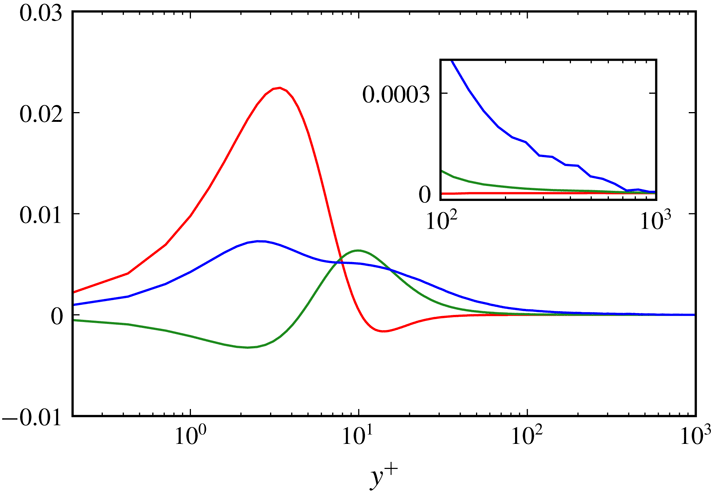
Wall-normal distribution of each term of (3.5) at the streamwise location corresponding to
 $Re_{\unicode[STIX]{x1D703}}=3170$
. Red,
 $2\overline{\overline{\unicode[STIX]{x1D714}_{i}}\unicode[STIX]{x1D61A}_{ij}^{\prime }\unicode[STIX]{x1D714}_{j}^{\prime }}^{+}$
; green,
 $\overline{\unicode[STIX]{x1D714}_{i}^{\prime }\overline{\unicode[STIX]{x1D61A}_{ij}}\unicode[STIX]{x1D714}_{j}^{\prime }}^{+}$
; blue,
 $\overline{\unicode[STIX]{x1D714}_{i}^{\prime }\unicode[STIX]{x1D61A}_{ij}^{\prime }\unicode[STIX]{x1D714}_{j}^{\prime }}^{+}$
. The inset shows the close-up for the range
 $10^{2}\leqslant y^{+}\leqslant 10^{3}$
.

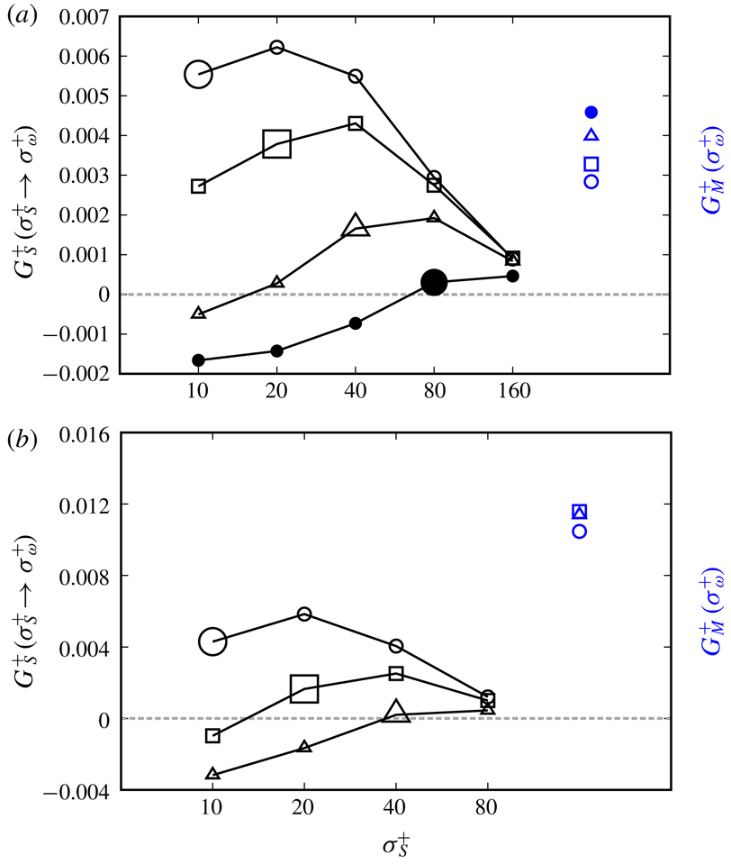
Contribution (3.6) of the strain rate coarse-grained at
 $\unicode[STIX]{x1D70E}_{S}$
to the stretching of vortices at
 $\unicode[STIX]{x1D70E}_{\unicode[STIX]{x1D714}}^{+}=10~(\circ )$
,
 $20~(\Box )$
,
 $40~(\triangle )$
,
 $80~(\bullet )$
and
 $160~(\blacksquare )$
for
 $Re_{\unicode[STIX]{x1D703}}=3170$
at (a)
 $y^{+}=300$
, (b)
 $100$
and (c)
 $40$
. The larger symbols correspond to the self-contribution (
 $\unicode[STIX]{x1D70E}_{s}^{+}=\unicode[STIX]{x1D70E}_{\unicode[STIX]{x1D714}}^{+}$
). Blue symbols indicate the contributions (3.7) from the mean stretching.

For a turbulent boundary layer,
 $$\begin{eqnarray}\displaystyle & \displaystyle \overline{\unicode[STIX]{x1D714}_{1}}=\overline{\unicode[STIX]{x1D714}_{2}}=0, & \displaystyle\end{eqnarray}$$
 $$\begin{eqnarray}\displaystyle & \displaystyle \overline{\unicode[STIX]{x1D61A}_{13}}=\overline{\unicode[STIX]{x1D61A}_{31}}=\overline{\unicode[STIX]{x1D61A}_{23}}=\overline{\unicode[STIX]{x1D61A}_{32}}=\overline{\unicode[STIX]{x1D61A}_{33}}=0, & \displaystyle\end{eqnarray}$$
where
 $$\begin{eqnarray}\unicode[STIX]{x1D714}_{i}=\overline{\unicode[STIX]{x1D714}_{i}}+\unicode[STIX]{x1D714}_{i}^{\prime },\quad \unicode[STIX]{x1D61A}_{ij}=\overline{\unicode[STIX]{x1D61A}_{ij}}+\unicode[STIX]{x1D61A}_{ij}^{\prime }.\end{eqnarray}$$
Here, the overbar
 $\overline{\,\cdot \,}$
denotes the average in the spanwise direction and time, the prime
 $\cdot \,^{\prime }$
denotes the deviation from the mean, and the subscripts
 $1$
,
 $2$
and
 $3$
denote the
 $x$
,
 $y$
and
 $z$
directions, respectively. Substituting (3.4) into the production term on the right-hand side of (3.1) and taking the average, we can rewrite it as
 $$\begin{eqnarray}\displaystyle \overline{\unicode[STIX]{x1D714}_{i}\unicode[STIX]{x1D61A}_{ij}\unicode[STIX]{x1D714}_{j}}=2\overline{\overline{\unicode[STIX]{x1D714}_{i}}\unicode[STIX]{x1D61A}_{ij}^{\prime }\unicode[STIX]{x1D714}_{j}^{\prime }}+\overline{\unicode[STIX]{x1D714}_{i}^{\prime }\overline{\unicode[STIX]{x1D61A}_{ij}}\unicode[STIX]{x1D714}_{j}^{\prime }}+\overline{\unicode[STIX]{x1D714}_{i}^{\prime }\unicode[STIX]{x1D61A}_{ij}^{\prime }\unicode[STIX]{x1D714}_{j}^{\prime }}. & & \displaystyle\end{eqnarray}$$
Here, we have used (3.2) and (3.3).
In figure 5, we show the wall-normal distribution of each term of (3.5) at the streamwise location corresponding to
 $Re_{\unicode[STIX]{x1D703}}=3170$
. The first term
 $2\overline{\overline{\unicode[STIX]{x1D714}_{i}}\unicode[STIX]{x1D61A}_{ij}^{\prime }\unicode[STIX]{x1D714}_{j}^{\prime }}$
(red line) is important only in the viscous sublayer, and it has a positive peak at
 $y^{+}\approx 3$
.
The second and third terms are more important for the generation mechanism of vortices in the buffer and log layers. The second term
 $\overline{\unicode[STIX]{x1D714}_{i}^{\prime }\overline{\unicode[STIX]{x1D61A}_{ij}}\unicode[STIX]{x1D714}_{j}^{\prime }}$
has a peak at
 $y^{+}\approx 10$
, and it decreases away from the wall. This trend means that the enstrophy produced by the strain-rate fields induced by the mean velocity is dominant in the buffer layer. As will be shown below, this corresponds to the event that the mean flow stretches the vortices in the buffer layer. However, this effect becomes less important in the log layer (
 $y^{+}\gtrsim 10^{2}$
), where the third term
 $\overline{\unicode[STIX]{x1D714}_{i}^{\prime }\unicode[STIX]{x1D61A}_{ij}^{\prime }\unicode[STIX]{x1D714}_{j}^{\prime }}$
is the largest. In other words, the enstrophy in the log layer, where a hierarchy of vortices exists, is generated predominantly by the stretching by the turbulent fluctuation rather than the mean flow.
Next, we investigate the scale dependence of the contribution of the rate-of-strain tensor to the enstrophy production. For this purpose, we introduce a quantity
 $$\begin{eqnarray}\displaystyle G_{S}(\unicode[STIX]{x1D70E}_{S}\rightarrow \unicode[STIX]{x1D70E}_{\unicode[STIX]{x1D714}})=\overline{\left.\left(\frac{\unicode[STIX]{x1D714}_{i}^{\prime (\unicode[STIX]{x1D70E}_{\unicode[STIX]{x1D714}})}\unicode[STIX]{x1D61A}_{ij}^{\prime (\unicode[STIX]{x1D70E}_{S})}\unicode[STIX]{x1D714}_{j}^{\prime (\unicode[STIX]{x1D70E}_{\unicode[STIX]{x1D714}})}}{|\unicode[STIX]{x1D714}_{i}^{\prime (\unicode[STIX]{x1D70E}_{\unicode[STIX]{x1D714}})}|^{2}}\right)\right|}_{Q^{(\unicode[STIX]{x1D70E}_{\unicode[STIX]{x1D714}})}>0}, & & \displaystyle\end{eqnarray}$$
where
 $\unicode[STIX]{x1D714}_{i}^{\prime (\unicode[STIX]{x1D70E}_{\unicode[STIX]{x1D714}})}$
is the fluctuation vorticity coarse-grained at the scale
 $\unicode[STIX]{x1D70E}_{\unicode[STIX]{x1D714}}$
, and
 $\unicode[STIX]{x1D61A}_{ij}^{\prime (\unicode[STIX]{x1D70E}_{S})}$
is the fluctuation rate-of-strain tensor coarse-grained at the scale
 $\unicode[STIX]{x1D70E}_{S}$
, both of which are calculated from the coarse-grained fluctuation velocity
 $\tilde{u} _{i}^{\prime }$
at
 $\unicode[STIX]{x1D70E}$
. Since
 $G_{S}(\unicode[STIX]{x1D70E}_{S}\rightarrow \unicode[STIX]{x1D70E}_{\unicode[STIX]{x1D714}})$
indicates the contribution of the strain rates coarse-grained at
 $\unicode[STIX]{x1D70E}_{S}$
to the stretching of the vortices coarse-grained at
 $\unicode[STIX]{x1D70E}_{\unicode[STIX]{x1D714}}$
, if
 $G_{S}(\unicode[STIX]{x1D70E}_{S}\rightarrow \unicode[STIX]{x1D70E}_{\unicode[STIX]{x1D714}})$
is positive (negative), it indicates the stretch (contraction) of the vortices. A similar quantity was defined by Goto et al. (Reference Goto, Saito and Kawahara2017) for turbulence in a periodic cube. Here, in order to evaluate the stretching of the vortices identified by the
 $Q$
criterion, we use the average conditioned by
 $Q^{(\unicode[STIX]{x1D70E}_{\unicode[STIX]{x1D714}})}>0$
. In addition, we also define contributions from the mean flow stretching as
 $$\begin{eqnarray}\displaystyle G_{M}(\unicode[STIX]{x1D70E}_{\unicode[STIX]{x1D714}})=\overline{\left.\left(\frac{\unicode[STIX]{x1D714}_{i}^{\prime (\unicode[STIX]{x1D70E}_{\unicode[STIX]{x1D714}})}\overline{\unicode[STIX]{x1D61A}_{ij}}\unicode[STIX]{x1D714}_{j}^{\prime (\unicode[STIX]{x1D70E}_{\unicode[STIX]{x1D714}})}}{|\unicode[STIX]{x1D714}_{i}^{\prime (\unicode[STIX]{x1D70E}_{\unicode[STIX]{x1D714}})}|^{2}}\right)\right|}_{Q^{(\unicode[STIX]{x1D70E}_{\unicode[STIX]{x1D714}})}>0}. & & \displaystyle\end{eqnarray}$$
Same as in figure 6 at (a)
 $y^{+}=160$
and (b)
 $y^{+}=60$
(i.e.
 $y/\unicode[STIX]{x1D6FF}_{99}\approx 0.3$
) for lower Reynolds numbers (a)
 $Re_{\unicode[STIX]{x1D703}}=1640$
and (b)
 $440$
.

We evaluate these quantities defined by (3.6) and (3.7) at a streamwise location corresponding to
 $Re_{\unicode[STIX]{x1D703}}=3170$
. Results are plotted in figure 6 for three heights from the wall, (a)
 $y^{+}=300$
, (b)
 $100$
and (c)
 $40$
. Looking at the open symbols in figure 6(a), we can see that for smaller scales (i.e.
 $\unicode[STIX]{x1D70E}_{\unicode[STIX]{x1D714}}^{+}=10$
,
 $20$
and
 $40$
) the contribution
 $G_{S}(2\unicode[STIX]{x1D70E}_{\unicode[STIX]{x1D714}}\rightarrow \unicode[STIX]{x1D70E}_{\unicode[STIX]{x1D714}})$
from the strain-rate fields of twice-larger scales is the most significant. It is also seen that the contribution
 $G_{M}(\unicode[STIX]{x1D70E}_{\unicode[STIX]{x1D714}})$
from the mean shear (blue symbols) is less important than
 $G_{S}(2\unicode[STIX]{x1D70E}_{\unicode[STIX]{x1D714}}\rightarrow \unicode[STIX]{x1D70E}_{\unicode[STIX]{x1D714}})$
. In contrast, for larger scales (i.e.
 $\unicode[STIX]{x1D70E}_{\unicode[STIX]{x1D714}}^{+}=80$
and
 $160$
), denoted by closed symbols in figure 6(a), the contribution
 $G_{M}(\unicode[STIX]{x1D70E}_{\unicode[STIX]{x1D714}})$
from the mean shear is larger than
 $G_{S}(\unicode[STIX]{x1D70E}_{S}\rightarrow \unicode[STIX]{x1D70E}_{\unicode[STIX]{x1D714}})$
. These trends observed for the height
 $y^{+}=300$
(figure 6
a) are valid also for the height
 $y^{+}=100$
(figure 6
b). Therefore, an important conclusion drawn from figure 6(a,b) is that, in the log layer, the strain rates at the scale that is twice as large as the stretched vortices, rather than the mean flow, contribute most to the stretching of the small-scale vortices (say,
 $\unicode[STIX]{x1D70E}_{\unicode[STIX]{x1D714}}^{+}\lesssim y^{+}/5$
; see figure 10 and the discussion of the figure). In the buffer layer, on the other hand, the mean-flow stretching is more important than the contribution from the strain-rate fields induced by the other scales. The evidence is given in figure 6(c), where the results for
 $y^{+}=40$
are shown. Among the contributions from the fluctuating strain-rate fields, the twice-larger scale contributes the most, but
 $G_{S}(2\unicode[STIX]{x1D70E}_{\unicode[STIX]{x1D714}}\rightarrow \unicode[STIX]{x1D70E}_{\unicode[STIX]{x1D714}})$
is smaller than the contribution
 $G_{M}(\unicode[STIX]{x1D70E}_{\unicode[STIX]{x1D714}})$
from the mean shear. In summary, the mean flow contributes most to the stretching of large-scale vortices, i.e. the vortices whose size is of the order of the distance from the wall.
For comparison, we show in figure 7 results for relatively low Reynolds numbers
 $Re_{\unicode[STIX]{x1D703}}=1640$
(figure 7
a) and
 $Re_{\unicode[STIX]{x1D703}}=440$
(figure 7
b). Both results are for a height
 $y/\unicode[STIX]{x1D6FF}_{99}\approx 0.3$
. The result for
 $Re_{\unicode[STIX]{x1D703}}=440$
is obtained by another DNS (see appendix A). Similarly to the higher-Reynolds-number cases, among the contributions from fluctuating strain-rate fields, those twice as large as the stretched vortices contribute most significantly. However, the lower the Reynolds number is, the larger the contribution to the vortex stretching from the mean flow becomes.
We have shown that small-scale vortices are stretched predominantly either by the mean flow or by the strain-rate fields at the scale twice as large as themselves. The dominance depends on the distance from the wall, the size of the vortices and the Reynolds number. To quantitatively evaluate the dominance, we define the ratio
 $$\begin{eqnarray}\displaystyle \unicode[STIX]{x1D6E4}(\unicode[STIX]{x1D70E}_{\unicode[STIX]{x1D714}})=\frac{G_{S}(2\unicode[STIX]{x1D70E}_{\unicode[STIX]{x1D714}}\rightarrow \unicode[STIX]{x1D70E}_{\unicode[STIX]{x1D714}})}{G_{M}(\unicode[STIX]{x1D70E}_{\unicode[STIX]{x1D714}})} & & \displaystyle\end{eqnarray}$$
of the contribution
 $G_{S}(2\unicode[STIX]{x1D70E}_{\unicode[STIX]{x1D714}}\rightarrow \unicode[STIX]{x1D70E}_{\unicode[STIX]{x1D714}})$
of the coarse-grained strain rates to the stretching of the vortices coarse-grained at their half-scale and the contribution
 $G_{M}(\unicode[STIX]{x1D70E}_{\unicode[STIX]{x1D714}})$
of the mean flow. Here, we note that
 $\unicode[STIX]{x1D6E4}$
as well as
 $G_{S}$
and
 $G_{M}$
are functions not only of
 $\unicode[STIX]{x1D70E}_{\unicode[STIX]{x1D714}}$
but also of
 $y^{+}$
and
 $Re_{\unicode[STIX]{x1D703}}$
. For brevity, however, we omit the arguments
 $y^{+}$
and
 $Re_{\unicode[STIX]{x1D703}}$
of
 $\unicode[STIX]{x1D6E4}$
. When
 $\unicode[STIX]{x1D6E4}(\unicode[STIX]{x1D70E}_{\unicode[STIX]{x1D714}})>1$
, the vortices at
 $\unicode[STIX]{x1D70E}_{\unicode[STIX]{x1D714}}$
are stretched predominantly by the strain rates twice as large as themselves; otherwise, they are stretched mainly by the mean flow.
Let us first investigate
 $\unicode[STIX]{x1D6E4}$
for the smallest-scale vortices. Figure 8 shows the results for
 $\unicode[STIX]{x1D6E4}(\unicode[STIX]{x1D70E}_{\unicode[STIX]{x1D714}}^{+}=10)$
as a function of
 $Re_{\unicode[STIX]{x1D703}}$
and height
 $y^{+}$
. The ratio
 $\unicode[STIX]{x1D6E4}$
is less than
 $1$
for
 $y^{+}\lesssim 40$
for any Reynolds numbers, which means that the contribution to the stretching from the mean flow is larger for
 $y^{+}\lesssim 40$
, that is, even the very small vortices (
 $\unicode[STIX]{x1D70E}_{\unicode[STIX]{x1D714}}^{+}=10$
) in the buffer layer are stretched directly by the mean flow (see also figure 6
c). In contrast, in the log layer (
 $y^{+}\gtrsim 100$
),
 $\unicode[STIX]{x1D6E4}$
is greater than
 $1$
, which means that the contribution from the strain-rate fields induced by the twice-larger scale is more significant than from the mean shear.
The ratio (3.8) between the contribution of strain rate coarse-grained at
 $\unicode[STIX]{x1D70E}_{S}^{+}=20$
to the stretching of vortices coarse-grained at
 $\unicode[STIX]{x1D70E}_{\unicode[STIX]{x1D714}}^{+}=10$
and the contribution of the mean flow as a function of
 $Re_{\unicode[STIX]{x1D703}}$
and the height
 $y^{+}$
. The blue line indicates the crossover (
 $\unicode[STIX]{x1D6E4}=1$
) of the dominance of the stretching from the mean flow to large-scale vortices. Only the region
 $y^{+}<\unicode[STIX]{x1D6FF}_{99}^{+}$
is plotted.

Taylor-length-based Reynolds number
 $Re_{\unicode[STIX]{x1D706}}$
as a function of
 $Re_{\unicode[STIX]{x1D703}}$
and
 $y^{+}$
. Only the region
 $y^{+}<\unicode[STIX]{x1D6FF}_{99}^{+}$
is plotted.

To explain these observation, we plot the Taylor-length-based Reynolds number
 $Re_{\unicode[STIX]{x1D706}}=u_{rms}^{\prime }\unicode[STIX]{x1D706}/\unicode[STIX]{x1D708}$
as a function of
 $Re_{\unicode[STIX]{x1D703}}$
and
 $y^{+}$
in figure 9. Here, the Taylor length is defined by
 $$\begin{eqnarray}\displaystyle \unicode[STIX]{x1D706}=\sqrt{\frac{{u_{rms}^{\prime }}^{2}}{\,\overline{(\unicode[STIX]{x2202}u^{\prime }/\unicode[STIX]{x2202}z)^{2}}\,}}. & & \displaystyle\end{eqnarray}$$
Comparing figures 8 and 9, we see that, in the buffer and log layers,
 $\unicode[STIX]{x1D6E4}$
is larger when
 $Re_{\unicode[STIX]{x1D706}}$
is larger. More precisely, in the buffer layer (say,
 $y^{+}\lesssim 40$
),
 $Re_{\unicode[STIX]{x1D706}}$
is always smaller than
 $50$
, which means that there is no scale separation, and
 $\unicode[STIX]{x1D6E4}$
is always smaller than
 $1$
, which means that all vortices in the buffer layer are directly stretched by mean shear (figures 6
c, 7
b and 8). Figure 8 also shows that the crossover
 $\unicode[STIX]{x1D6E4}(\unicode[STIX]{x1D70E}_{\unicode[STIX]{x1D714}}^{+}=10)\gtrless 1$
(the blue line in figure 8) occurs at
 $y^{+}$
between
 $40$
and
 $60$
. According to figure 9, this corresponds to
 $Re_{\unicode[STIX]{x1D706}}\approx 50$
. This value of
 $Re_{\unicode[STIX]{x1D706}}$
is reasonable, since it is known that the inertial range starts to appear for
 $Re_{\unicode[STIX]{x1D706}}\gtrsim 50$
. Furthermore, we can confirm that, for the locations with
 $Re_{\unicode[STIX]{x1D706}}\gtrsim 50$
(figure 9),
 $\unicode[STIX]{x1D6E4}(\unicode[STIX]{x1D70E}_{\unicode[STIX]{x1D714}}^{+}=10)$
is always larger than
 $1$
(figure 8). Note that such points are located only in the log layer for
 $Re_{\unicode[STIX]{x1D703}}\gtrsim 1000$
. We emphasize that
 $\unicode[STIX]{x1D6E4}$
is always smaller than
 $1$
for any heights (except for the outer layer) when
 $Re_{\unicode[STIX]{x1D703}}\lesssim 500$
(figure 7
b).
The ratio (3.8) between the contribution of strain rates coarse-grained at
 $2\unicode[STIX]{x1D70E}_{\unicode[STIX]{x1D714}}^{+}$
to the stretching of vortices coarse-grained at
 $\unicode[STIX]{x1D70E}_{\unicode[STIX]{x1D714}}^{+}$
and the contribution of the mean flow as a function of
 $\unicode[STIX]{x1D70E}_{\unicode[STIX]{x1D714}}^{+}$
and
 $y^{+}$
for
 $Re_{\unicode[STIX]{x1D703}}=3170$
. Blue line, the crossover (
 $\unicode[STIX]{x1D6E4}=1$
) of the dominance of the stretching from the mean flow to large-scale vortices; red line,
 $\unicode[STIX]{x1D70E}_{\unicode[STIX]{x1D714}}=5\unicode[STIX]{x1D702}$
; green dotted line,
 $\unicode[STIX]{x1D70E}_{\unicode[STIX]{x1D714}}=0.7L_{c}$
; black dashed line,
 $\unicode[STIX]{x1D70E}_{\unicode[STIX]{x1D714}}=y/5$
. The contours are plotted by the interpolation of
 $\unicode[STIX]{x1D6E4}$
evaluated for the four cases (
 $\unicode[STIX]{x1D70E}_{\unicode[STIX]{x1D714}}^{+}=10$
,
 $20$
,
 $40$
and
 $80$
).

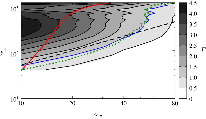
In figure 8, we have examined the contribution ratio
 $\unicode[STIX]{x1D6E4}$
(3.8) between the vortex stretching by twice-larger-scale vortices and the mean-flow stretching for the smallest scale (
 $\unicode[STIX]{x1D70E}_{\unicode[STIX]{x1D714}}^{+}=10$
) in the flow. However, although the scale (
 $\unicode[STIX]{x1D70E}_{\unicode[STIX]{x1D714}}^{+}=10$
) is smallest in the buffer layer, it is not necessarily smallest in the log layer. Therefore in figure 10 we show
 $\unicode[STIX]{x1D6E4}$
as a function of the filter scale
 $\unicode[STIX]{x1D70E}_{\unicode[STIX]{x1D714}}^{+}$
(namely, the size of vortices) and
 $y^{+}$
for a given Reynolds number (
 $Re_{\unicode[STIX]{x1D703}}=3170$
). The red line indicates
 $\unicode[STIX]{x1D70E}_{\unicode[STIX]{x1D714}}=5\unicode[STIX]{x1D702}$
as a function of
 $y^{+}$
. Since
 $5\unicode[STIX]{x1D702}$
is approximately the radius of the Kolmogorov-scale vortex tubes, we should look at
 $\unicode[STIX]{x1D6E4}$
in the region
 $\unicode[STIX]{x1D70E}_{\unicode[STIX]{x1D714}}\gtrsim 5\unicode[STIX]{x1D702}$
. For example,
 $\unicode[STIX]{x1D6E4}$
on the red line shows the dominance of the contribution to the stretching of the smallest vortices at each height. Looking at the value of
 $\unicode[STIX]{x1D6E4}$
on the red line, we see that the crossover (
 $\unicode[STIX]{x1D6E4}\gtrless 1$
) occurs at
 $y^{+}\approx 50$
, which is approximately the lower boundary of the log layer. It is also interesting to observe that the crossover (blue line) occurs at the height
 $y^{+}\approx 5\unicode[STIX]{x1D70E}_{\unicode[STIX]{x1D714}}^{+}$
(black dashed line) for
 $y^{+}\lesssim 200$
(within the log layer), but this scaling does not hold in the outer layer (
 $y^{+}\gtrsim 200$
for this
 $Re_{\unicode[STIX]{x1D703}}$
). It is important to show that the height
 $y$
where
 $\unicode[STIX]{x1D6E4}=1$
is proportional to the Corrsin scale
 $L_{c}$
(Corrsin Reference Corrsin1958; Jiménez Reference Jiménez2013), which is defined by
 $L_{c}=\overline{\unicode[STIX]{x1D716}}^{1/2}S^{-3/2}$
with
 $S$
being the shear rate of the mean flow. In figure 10, the green dotted line indicates
 $0.7L_{c}$
, which is in good agreement with the blue line (
 $\unicode[STIX]{x1D6E4}=1$
). This observation is reasonable because the shearing time scale
 $S^{-1}$
and the cascade time scale (i.e. the eddy turnover time)
 $\ell ^{2/3}\hspace{2.22198pt}\overline{\unicode[STIX]{x1D716}}^{-1/3}$
are balanced at
 $\ell \approx L_{c}$
. Incidentally, Jiménez (Reference Jiménez2013) concluded that
 $L_{c}\approx 0.3y$
in the log layer, which is consistent with the above observation that the size
 $\unicode[STIX]{x1D70E}_{\unicode[STIX]{x1D714}}$
of vortices for
 $\unicode[STIX]{x1D6E4}=1$
is approximately
 $y/5$
(
 ${\approx}(2/3)L_{c}\approx 0.7L_{c}$
). In summary, figure 10 shows that
 $\unicode[STIX]{x1D6E4}<1$
in the buffer layer even for higher
 $Re_{\unicode[STIX]{x1D703}}$
(see also figures 6
c, 7
b and 8), whereas, in the log layer,
 $\unicode[STIX]{x1D6E4}>1$
in the scales between the red (
 $5\unicode[STIX]{x1D702}$
) and blue (
 $y/5\approx 0.7L_{c}$
) lines.
3.3 Alignment of vorticity and eigenvectors of rate-of-strain tensor
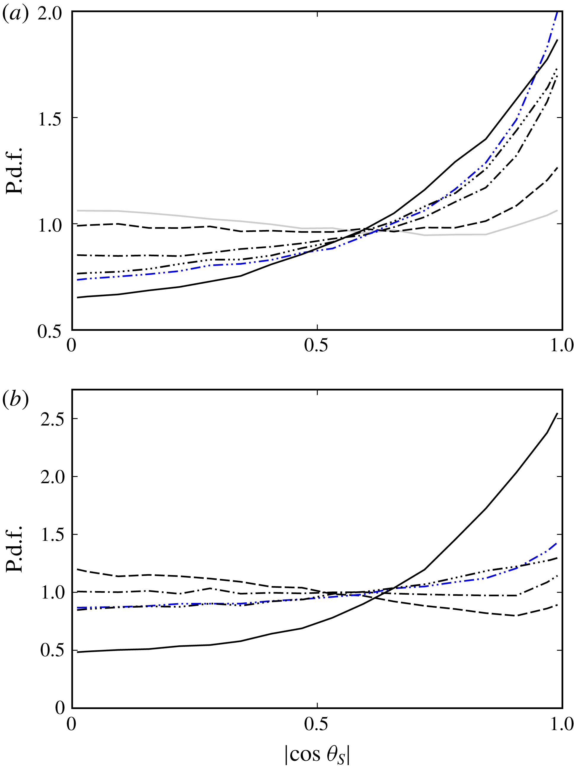
Conditional p.d.f. of the alignment between the vorticity coarse-grained at (a)
 $\unicode[STIX]{x1D70E}_{\unicode[STIX]{x1D714}}^{+}=20$
(
 $\unicode[STIX]{x1D70E}_{\unicode[STIX]{x1D714}}\approx 6\unicode[STIX]{x1D702}$
) and (b)
 $\unicode[STIX]{x1D70E}_{\unicode[STIX]{x1D714}}^{+}=10$
(
 $\unicode[STIX]{x1D70E}_{\unicode[STIX]{x1D714}}\approx 4\unicode[STIX]{x1D702}$
) and the first eigenvector of the rate-of-strain tensor coarse-grained at
 $\unicode[STIX]{x1D70E}_{S}=1/2\unicode[STIX]{x1D70E}_{\unicode[STIX]{x1D714}}$
(grey solid line),
 $\unicode[STIX]{x1D70E}_{S}=\unicode[STIX]{x1D70E}_{\unicode[STIX]{x1D714}}$
(dashed line),
 $\unicode[STIX]{x1D70E}_{S}=2\unicode[STIX]{x1D70E}_{\unicode[STIX]{x1D714}}$
(dot-dashed line),
 $\unicode[STIX]{x1D70E}_{S}=4\unicode[STIX]{x1D70E}_{\unicode[STIX]{x1D714}}$
(double dot-dashed line, blue) and
 $\unicode[STIX]{x1D70E}_{S}=8\unicode[STIX]{x1D70E}_{\unicode[STIX]{x1D714}}$
(triple dot-dashed line) at two different positions: (a)
 $y^{+}=300$
for
 $Re_{\unicode[STIX]{x1D703}}=3170$
; and (b)
 $y^{+}=60$
for
 $Re_{\unicode[STIX]{x1D703}}=440$
. The black solid line denotes the conditional p.d.f. of
 $|\!\cos \unicode[STIX]{x1D703}_{M}|$
.
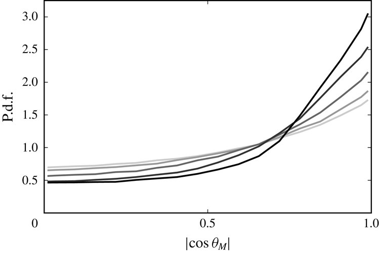
Conditional p.d.f. of the alignment between the vorticity coarse-grained at
 $\unicode[STIX]{x1D70E}_{\unicode[STIX]{x1D714}}^{+}=10$
(very light grey),
 $\unicode[STIX]{x1D70E}_{\unicode[STIX]{x1D714}}^{+}=20$
(light grey),
 $\unicode[STIX]{x1D70E}_{\unicode[STIX]{x1D714}}^{+}=40$
(grey),
 $\unicode[STIX]{x1D70E}_{\unicode[STIX]{x1D714}}^{+}=80$
(dark grey) and
 $\unicode[STIX]{x1D70E}_{\unicode[STIX]{x1D714}}^{+}=160$
(black) and the stretching direction of the mean flow at
 $y^{+}=300$
for
 $Re_{\unicode[STIX]{x1D703}}=3170$
.

We rewrite the production term of the fluctuation enstrophy as
 $$\begin{eqnarray}\displaystyle \frac{\unicode[STIX]{x1D714}_{i}^{\prime }\unicode[STIX]{x1D61A}_{ij}^{\prime }\unicode[STIX]{x1D714}_{j}^{\prime }}{|\unicode[STIX]{x1D714}_{i}^{\prime }|^{2}}=s_{i}^{\prime }({\widehat{\boldsymbol{e}}_{i}}^{\prime }\boldsymbol{\cdot }\widehat{\unicode[STIX]{x1D74E}}^{\prime })^{2}, & & \displaystyle\end{eqnarray}$$
where
 $s_{i}^{\prime }$
(
 $s_{1}^{\prime }\geqslant s_{2}^{\prime }\geqslant s_{3}^{\prime }$
) are the eigenvalues of the fluctuation rate-of-strain tensor
 $\unicode[STIX]{x1D61A}_{ij}^{\prime }$
,
 ${\widehat{\boldsymbol{e}}_{i}}^{\prime }$
are the corresponding eigenvectors, and
 $\widehat{\unicode[STIX]{x1D74E}}^{\prime }$
is the normalized vorticity
 $\widehat{\unicode[STIX]{x1D74E}}^{\prime }=\unicode[STIX]{x1D74E}^{\prime }/\unicode[STIX]{x1D714}^{\prime }$
. Since
 $s_{1}^{\prime }+s_{2}^{\prime }+s_{3}^{\prime }=0$
for incompressible fluids,
 ${\widehat{\boldsymbol{e}}_{1}}^{\prime }$
corresponds to the direction with maximum stretching. In this section, we investigate the alignment between the vorticity and the stretching direction so that we can further clarify the picture of the vortex stretching in a turbulent boundary layer. For this purpose, we evaluate the probability density function (p.d.f.) of
 $$\begin{eqnarray}\displaystyle \cos \unicode[STIX]{x1D703}_{S}={\widehat{\boldsymbol{e}}_{1}}^{\,\prime (\unicode[STIX]{x1D70E}_{S})}\,\boldsymbol{\cdot }\,\widehat{\unicode[STIX]{x1D74E}}^{\prime (\unicode[STIX]{x1D70E}_{\unicode[STIX]{x1D714}})}, & & \displaystyle\end{eqnarray}$$
where
 ${\widehat{\boldsymbol{e}}_{1}}^{\,\prime (\unicode[STIX]{x1D70E}_{S})}$
is the stretching direction of the fluctuation rate-of-strain tensor coarse-grained at scale
 $\unicode[STIX]{x1D70E}_{S}$
and
 $\widehat{\unicode[STIX]{x1D74E}}^{\prime (\unicode[STIX]{x1D70E}_{\unicode[STIX]{x1D714}})}$
is the normalized fluctuation vorticity coarse-grained at scale
 $\unicode[STIX]{x1D70E}_{\unicode[STIX]{x1D714}}$
. We investigate the tendency of the alignment between the vortices at
 $\unicode[STIX]{x1D70E}_{\unicode[STIX]{x1D714}}$
and the stretching direction at
 $\unicode[STIX]{x1D70E}_{S}$
by calculating the p.d.f. of (3.11) using the conditional average for
 $Q^{(\unicode[STIX]{x1D70E}_{\unicode[STIX]{x1D714}})}>0$
in the same way as in § 3.2. We also investigate the conditional p.d.f. of
 $$\begin{eqnarray}\displaystyle \cos \unicode[STIX]{x1D703}_{M}=\bar{\boldsymbol{e}}_{1}\,\boldsymbol{\cdot }\,\widehat{\unicode[STIX]{x1D74E}}^{\prime (\unicode[STIX]{x1D70E}_{\unicode[STIX]{x1D714}})}, & & \displaystyle\end{eqnarray}$$
where
 $\bar{\boldsymbol{e}}_{1}$
denotes the stretching direction of the mean flow.
Fixing the filter scale
 $\unicode[STIX]{x1D70E}_{\unicode[STIX]{x1D714}}$
of the vorticity, we evaluate the conditional p.d.f. of
 $|\cos \unicode[STIX]{x1D703}_{S}|$
for various
 $\unicode[STIX]{x1D70E}_{S}$
for two different Reynolds numbers (figure 11
a,
 $Re_{\unicode[STIX]{x1D703}}=3170$
; figure 11
b,
 $Re_{\unicode[STIX]{x1D703}}=440$
). Figure 11(a) shows the result for the small scale (
 $\unicode[STIX]{x1D70E}_{\unicode[STIX]{x1D714}}^{+}=20$
) at
 $y^{+}=300$
(same as in figure 6
a) and figure 11(b) is for
 $\unicode[STIX]{x1D70E}_{\unicode[STIX]{x1D714}}^{+}=10$
at
 $y^{+}=60$
(same as in figure 7
b). In both cases, among different
 $\unicode[STIX]{x1D70E}_{S}$
, the tendency that
 ${\widehat{\boldsymbol{e}}_{1}}^{\,\prime (\unicode[STIX]{x1D70E}_{S})}\Vert \widehat{\unicode[STIX]{x1D74E}}^{\prime (\unicode[STIX]{x1D70E}_{\unicode[STIX]{x1D714}})}$
is the strongest for
 $\unicode[STIX]{x1D70E}_{S}^{+}=4\unicode[STIX]{x1D70E}_{\unicode[STIX]{x1D714}}^{+}$
(double dot-dashed blue lines in figure 11). Namely, the trend of parallel alignment between the vorticity at a small scale and the stretching direction at a scale four times as large is the strongest. This result is similar to the observation in decaying homogeneous isotropic turbulence that vortices at a given scale tend to align with the stretching direction at the scale
 $3$
–
 $5$
times as large as the given scale (Leung et al.
Reference Leung, Swaminathan and Davidson2012). Despite this result, it is the strain-rate scale twice as large as the vortices that are dominant (figures 6 and 7) because the stretching rate is larger for smaller scales.
However, looking at the black solid curves in figure 11, we notice that the tendency that the coarse-grained fluctuation vorticity is parallel to the stretching direction of the mean flow is also relatively strong even for the higher-Reynolds-number case (
 $Re_{\unicode[STIX]{x1D703}}=3170$
, figure 11
a). To investigate the scale dependence of the alignment between the coarse-grained fluctuation vorticity and the stretching direction of the mean flow, we plot the conditional p.d.f. of
 $|\cos \unicode[STIX]{x1D703}_{M}|$
for five different scales in figure 12. The Reynolds number and height are the same as in figure 11(a). Figure 12 shows that larger-scale vortices are more likely to align with the stretching direction of the mean flow. We confirm that this is the case also in the buffer layer (figures are omitted). This result is consistent with the fact that the contribution to the enstrophy production from the mean flow is larger for larger scales (figures 6 and 7). Note again that the enstrophy production depends not only on the alignment between the vorticity and the eigenvectors but also on the magnitude of the eigenvalues, and that the stretching rate is larger for smaller scales. Comparing the results for the two Reynolds numbers in figure 11, we also see that the parallel alignment of the vorticity with the stretching direction by the mean flow becomes more likely for lower Reynolds numbers. This is also consistent with the observation that the contribution to the stretching from the mean shear increases as the Reynolds number decreases (figure 7).
In summary, for larger scales at a given
 $Re_{\unicode[STIX]{x1D703}}$
, and for lower
 $Re_{\unicode[STIX]{x1D703}}$
at a given scale, vortices are more likely to align in the stretching direction of the mean shear. In other words, small-scale vortices become less aligned (i.e. more isotropic) as the Reynolds number increases, which is consistent with the visualization (figure 3). These are also consistent with the conclusions of the review by Jiménez (Reference Jiménez2013) that shear interacts with large-scale ‘eddies’, whereas small-scale vortices away from the wall decouple from the shear and become isotropic.
4 Discussion
4.1 Generation events of the hierarchy of multiscale vortices
Isosurfaces of the second invariant of the coarse-grained velocity gradient tensor. The coarse-graining scale is
 $\unicode[STIX]{x1D70E}^{\oplus }=80$
, the threshold is chosen as
 $m_{Q}+0.5s_{Q}~(=1.2\times 10^{-4})$
, and the Reynolds number changes as
 $Re_{\unicode[STIX]{x1D703}}=2670{-}3170$
. The flow is from lower left to upper right. The black grid width is
 $200$
wall units evaluated at the plane corresponding to
 $Re_{\unicode[STIX]{x1D703}}=2860$
, and the blue solid line indicates the
 $99\,\%$
boundary layer thickness
 $\unicode[STIX]{x1D6FF}_{99}$
.

In the previous section, we have quantitatively verified the scenario of the generation mechanism of the hierarchy of vortices. Namely, large-scale structures are stretched and created by mean velocity, whereas small-scale vortices in the log layer are generated and created by the large-scale vortices. It is therefore not difficult to find many concrete events in the physical space which are consistent with the quantitative results in §§ 3.2 and 3.3. Among them, we show the clearest examples in the following (figures 14 and 15).
First, we show in figure 13 a snapshot of isosurfaces of the second invariant
 $Q^{(\unicode[STIX]{x1D70E})}$
of the velocity gradient tensor coarse-grained at
 $\unicode[STIX]{x1D70E}^{\oplus }=80$
to identify large-scale vortices. We see that the large-scale vortices tend to align with the stretching direction of the mean flow, which is inclined at approximately
 $\unicode[STIX]{x03C0}/4$
from the streamwise direction. We also notice that the downstream part of the vortices is lifted up to the boundary layer thickness and some of them orient into the spanwise direction to form a hairpin-like structure. This observation is consistent with the alignment between large-scale vortices and the stretching direction induced by the mean flow (figure 12). Incidentally, as was shown in figure 3, the orientation of the smallest-scale vortices apart from the wall is random, which is also consistent with the p.d.f. shown in figure 11(a).
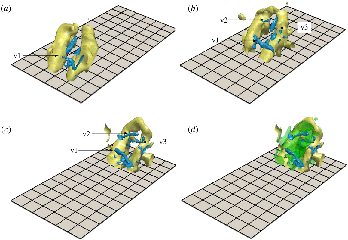
An example of the generation process of small-scale vortices (v1, v2 and v3) around a large-scale hairpin-like vortex. Only a small domain in figure 13 is shown. The flow is from lower left to upper right. The two different colours correspond to the isosurfaces of the second invariant of the velocity gradient tensor coarse-grained at two different scales: yellow,
 $\unicode[STIX]{x1D70E}^{\oplus }=80$
; and blue,
 $40$
. Thresholds are set as
 $m_{Q}+0.5s_{Q}$
. Time elapses as (a)
 $t^{\oplus }=0$
, (b)
 $30$
and (c)
 $74$
. (d) The isosurfaces of
 $\unicode[STIX]{x1D61A}_{ij}^{\prime (\unicode[STIX]{x1D70E})}\unicode[STIX]{x1D61A}_{ij}^{\prime (\unicode[STIX]{x1D70E})}$
coarse-grained at
 $\unicode[STIX]{x1D70E}^{\oplus }=80$
with the threshold
 $3.8\times 10^{-4}$
are also shown at the same time as in (c). The black grid width on the wall is the same as in figure 13. Small-scale vortices are visualized in the region
 $200\lesssim y^{+}\lesssim 670$
.

Next, let us look at generation events of small-scale vortices in the log layer. For this purpose, we educe a large-scale hairpin-like vortex and the surrounding small-scale vortices in figure 14. Here, we visualize the vortices only in a rectangular box whose faces are parallel to those of the computational domain to track the generation process of small-scale vortices around the large-scale vortex. The height of the visualization box for the large-scale vortex is
 $100\lesssim y^{+}\lesssim \unicode[STIX]{x1D6FF}_{99}^{+}$
and that for the small-scale vortices is
 $200\lesssim y^{+}\lesssim 670$
. The large-scale hairpin-like vortex (yellow) consists of two legs in the mean-flow-stretching direction and a spanwise head. The part of the spanwise head is approximately at the boundary layer thickness. By tracking this large-scale hairpin-like vortex in figure 14(a–c), we can see the generation process of small-scale vortices (v1, v2 and v3). Figure 14(d) shows the (green) isosurfaces of
 $\unicode[STIX]{x1D61A}_{ij}^{\prime (\unicode[STIX]{x1D70E})}\unicode[STIX]{x1D61A}_{ij}^{\prime (\unicode[STIX]{x1D70E})}$
coarse-grained at
 $\unicode[STIX]{x1D70E}^{\oplus }=80$
around the large-scale vortex. Noting that the legs of the large-scale hairpin-like vortex are a pair of counter-rotating vortices, we can see the reason why the strong strain-rate fields are created in the region, where the small-scale vortices (blue) are indeed stretched and amplified in the direction perpendicular to the legs. This is a typical example of small-scale vortex generation due to stretching by larger-scale vortices.
Other examples of the generation of small-scale structures in the log layer are shown in figure 15. The observed small-scale vortices (blue) are not the streamwise vortices stretched by the mean flow, but they are likely to be stretched by larger-scale strain rates in the same way as in figure 14. In particular, figure 15(a–c) shows the example for the one-legged hairpin-like vortex, and the small-scale vortex (v4) is generated by the nearby larger-scale vortex. Figure 15(d–f) shows that a quasi-streamwise (or one-legged hairpin-like) large-scale vortex stretches two small-scale vortices (v5 and v6) which never align to the stretching direction of the mean shear.
These concrete examples are consistent with the quantitative results that large-scale vortices are stretched and created by the mean flow and they tend to align with the mean shear (figure 13), whereas small-scale vortices apart from the wall are mainly stretched by the strain-rate field induced by large-scale vortices (figures 14 and 15). Here, it is worth mentioning that the shown small-scale vortex generation events in the log layer of the high-Reynolds-number turbulent boundary layer are qualitatively similar to those observed in turbulence in a periodic cube. We recall that the energy spectrum in the log layer approximately obeys the
 $-5/3$
power law (figure 2
a). In turbulence without a wall at sufficiently high Reynolds numbers, on each level of the hierarchy of vortices, vortex tubes tend to align with each other in an antiparallel manner (Goto et al.
Reference Goto, Saito and Kawahara2017). Since a pair of counter-rotating vortex tubes induces strongly shearing flows around it, such a pair of vortices effectively stretches and amplifies smaller-scale vortices. These events are similar to the vortex generation events around the legs of a hairpin-like vortex (figure 14). Furthermore, not only vortex pairs but also single vortex tubes can induce shear flow and create smaller-scale vortices (Hussain Reference Hussain1986; Melander & Hussain Reference Melander and Hussain1993). Such events are also similarly observed in the turbulent boundary layer (figure 15). These observations imply the similarity in the generation mechanism of small-scale vortices in these different turbulent flows, which might be an indication of small-scale universality. It is also worth mentioning that such generation events of small-scale vortices in a periodic cube are relevant to an energy cascading process (Goto Reference Goto2008). The observed events in figures 14 and 15 are therefore likely to correspond to the energy cascade process. However, more detailed investigations in terms of energy transfer in physical space are required to draw a solid conclusion on the energy cascade in a turbulent boundary layer. This is a near-future target of our studies.
Other examples of the generation process of small-scale vortices (v4, v5 and v6) around a large-scale (a–c) one-legged hairpin-like vortex and (d–f) stretching-direction vortex in figure 13. The flow is from lower left to upper right. The two different colours correspond to the isosurfaces of the second invariant of the velocity gradient tensor coarse-grained at two different scales: yellow,
 $\unicode[STIX]{x1D70E}^{\oplus }=80$
; blue,
 $40$
. Thresholds are set as
 $m_{Q}+0.5s_{Q}$
. Time elapses as (a)
 $t^{\oplus }=0$
, (b)
 $22$
, (c)
 $45$
, (d)
 $0$
, (e)
 $15$
and (f)
 $30$
. The black grid width on the wall is the same as in figure 13. Small-scale vortices are visualized in the region
 $450\lesssim y^{+}\lesssim 750$
.

4.2 Hairpin vortices
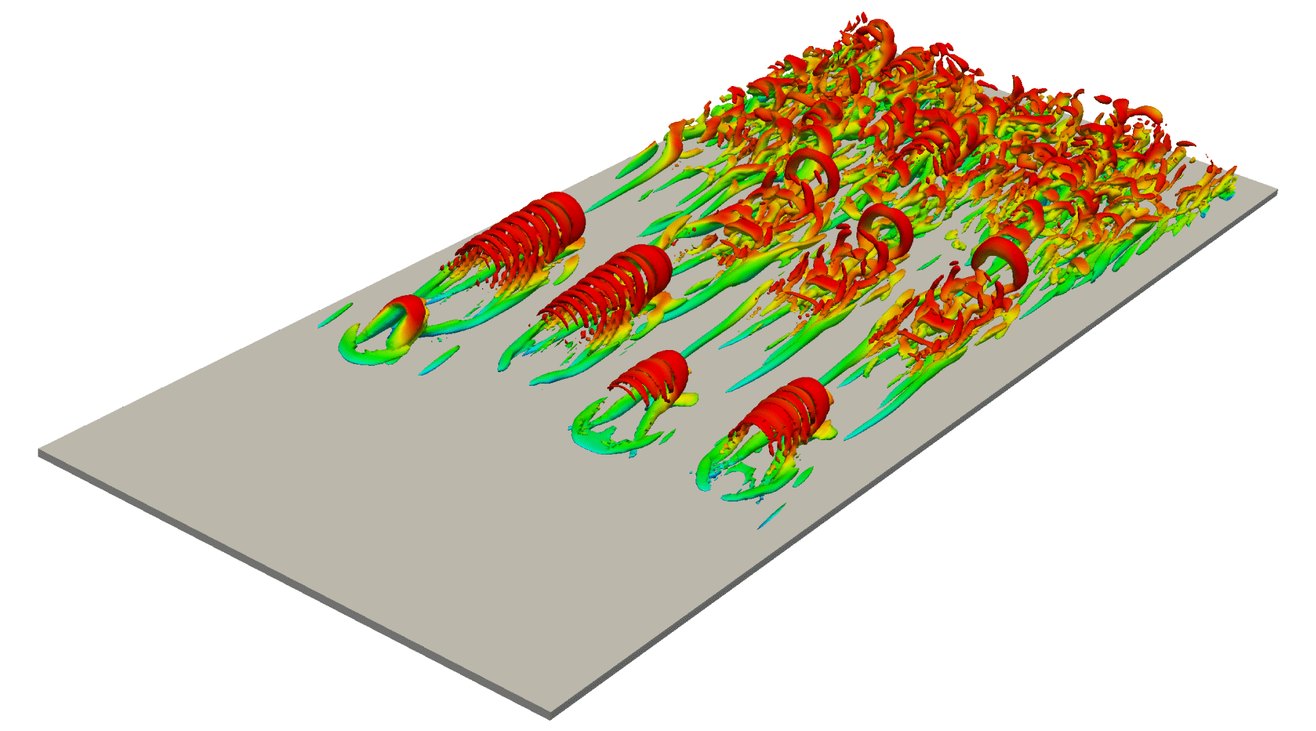
Although there is no objective definition of a hairpin vortex (Eitel-Amor et al. Reference Eitel-Amor, Örlü, Schlatter and Flores2015), we frequently observe hairpin-like vortices in turbulent boundary layers (see figure 16 in appendix A, for example). In fact, since the hairpin vortices were proposed as coherent structures in turbulent boundary layers by Theodorsen (Reference Theodorsen1952), evidence has been presented by many numerical simulations (Robinson Reference Robinson1991; Chong et al. Reference Chong, Soria, Perry, Chacin, Cantwell and Na1998; Wu & Moin Reference Wu and Moin2009) and experiments (Head & Bandyopadhyay Reference Head and Bandyopadhyay1981; Perry & Chong Reference Perry and Chong1982; Christensen & Adrian Reference Christensen and Adrian2001; Ganapathisubramani, Longmire & Marusic Reference Ganapathisubramani, Longmire and Marusic2003; Adrian Reference Adrian2007; Dennis & Nickels Reference Dennis and Nickels2011a ; Jodai & Elsinga Reference Jodai and Elsinga2016). Moreover, Adrian (Reference Adrian2007) reported that the hairpin packet model is consistent with the attached eddy hypothesis proposed by Townsend (Reference Townsend1976), in which the size of the eddies increases linearly with the distance from the wall.
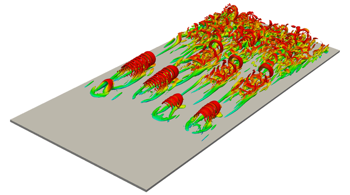
However, some DNS studies have reached the controversial conclusion that hairpin vortices are absent in developed turbulent boundary layers. Schlatter et al. (Reference Schlatter, Li, Örlü, Hussain and Henningson2014) showed that the hairpin vortices disappear by visualizing vortices and identifying the averaged structure with an objective vortex-eduction method when the Reynolds number increases. Jiménez et al. (Reference Jiménez, Hoyas, Simens and Mizuno2010) investigated the geometry of the vortical structures at moderate Reynolds numbers and concluded that it is hard to describe them as forests of hairpins (Wu & Moin Reference Wu and Moin2009). Eitel-Amor et al. (Reference Eitel-Amor, Örlü, Schlatter and Flores2015) also conducted the DNS of a turbulent boundary layer at relatively low Reynolds numbers, and reported that the flow is not dominated by hairpin vortices in a downstream region where turbulence is well developed. Our DNS also show similar results (see hairpin vortices for low Reynolds numbers in figure 16 and randomly oriented vortices for high Reynolds numbers in figure 3). Although quite a few hairpin vortex models were proposed to describe a turbulent boundary layer (Theodorsen Reference Theodorsen1952; Townsend Reference Townsend1976; Perry & Chong Reference Perry and Chong1982; Perry & Marusic Reference Perry and Marusic1995; Adrian, Meinhart & Tomkins Reference Adrian, Meinhart and Tomkins2000), it is unclear even whether the hairpin vortices exist.
Isosurfaces of the second invariant
 $Q^{+}~(=4.0\times 10^{-2})$
of the velocity gradient tensor. The colour indicates the streamwise velocity
 $u$
, ranging from
 $u=0$
(blue) to
 $u=U_{\infty }$
(red). Half of the spanwise direction of the computational domain is visualized. The Reynolds number
 $Re_{\unicode[STIX]{x1D703}}$
changes from
 $180$
to
 $370$
. The flow is from lower left to upper right.
The results shown in the present paper, however, imply that these previous observations are not necessarily conflicting. As shown in §§ 3.2 and 3.3, vortices with a size of the order of the height are directly stretched and amplified by the mean shear and form vortices in the direction of the mean-flow stretching. When such a pair of vortices is lifted up to the boundary layer thickness (i.e. turbulent/non-turbulent interface), the vortices are connected to the spanwise direction to form a hairpin-like vortex. In other words, only vortices with the size of the order of the boundary layer thickness can be hairpin-like vortices. In fact, this explains the observations. First, it is consistent with the disappearance of hairpin vortices in the buffer layer for higher Reynolds numbers. Although vortices in the buffer layer are directly stretched by the mean shear (figures 6 c, 7 b and 8), they cannot be lifted up to the boundary layer thickness. This is the reason why streamwise vortices, rather than hairpin vortices, are observed in the buffer layer at high Reynolds numbers (Jiménez Reference Jiménez2013). Second, small-scale vortices in the log layer are stretched and amplified by larger-scale fluctuating strain-rate fields (figures 6 a,b, 7 a and 8), and therefore their orientations are random (figures 3 and 11 a), and they cannot be hairpin vortices. Third, the largest-scale vortices (red ones in figure 4 and yellow ones in figures 13 and 14) in the log layer can be hairpin-shaped because they are directly stretched and amplified by the mean shear (figures 6 a,b and 7 a) and because they are as large as the boundary layer thickness. Indeed, some of the large-scale structures are hairpin-like (figures 4 c, 13 and 14). These observations are similar to those found by del Álamo et al. (Reference del Álamo, Jiménez, Zandonade and Moser2006) and Dennis & Nickels (Reference Dennis and Nickels2011a ). They identify large-scale hairpin vortices in the conditionally averaged fields. We emphasize that such large-scale vortices, identified in terms of velocity gradients, are not educed without coarse-graining. This is because the velocity gradients (and therefore their second invariant) take larger values for smaller scales. On the other hand, since velocity magnitudes take larger values for larger scale, the large-scale motions may be visible in terms of the velocity without coarse-graining and they are further clarified by (conditional) averaging to smooth out small-scale motions.
5 Conclusions
To understand the generation mechanism of multiscale vortical structures, we have conducted DNS of a turbulent boundary layer at high Reynolds numbers. Using the inlet flow condition provided by Lee et al. (Reference Lee, Jung, Sung and Zaki2013, Reference Lee, Sung and Zaki2017), we simulate turbulence at a Reynolds number high enough for the energy spectrum to show the Kolmogorov
 $-5/3$
power law and for the premultiplied energy spectrum to have the second peak (figure 2). We decompose the velocity field into the mean and fluctuations, and we further decompose the fluctuation fields into different scales by using the three-dimensional Gaussian filter (2.1). We then examine the contributions, defined by (3.6) and (3.7), to the enstrophy production term from the mean and scale-dependent fluctuation strain-rate fields to show the following. (i) In the log layer, vortices smaller than approximately one-fifth of the height are predominantly stretched and amplified by strain-rate fields at a scale twice as large as themselves, whereas larger vortices are directly stretched and amplified by the mean shear (figures 6
a,b and 7
a). (ii) In the buffer layer, all vortices are ‘large’ in the sense that they are as large as the height, and therefore they are stretched and amplified by the mean shear (figure 6
c). (iii) This is also the case for low Reynolds numbers (figure 7
b). The crossover of the dominance of the contributions from the mean to the turbulent fluctuations (figure 8) is explained in terms of the Taylor-length-based Reynolds number
 $Re_{\unicode[STIX]{x1D706}}$
(figure 9). More precisely,
 $Re_{\unicode[STIX]{x1D706}}$
must be larger than, at least,
 $50$
for even the smallest-scale vortices to be stretched and amplified by larger-scale strain-rate fields (rather than by the mean shear). This is consistent with the knowledge of homogeneous isotropic turbulence that the inertial range starts to appear for
 $Re_{\unicode[STIX]{x1D706}}\gtrsim 50$
. On the other hand, the upper bound of the size for vortices to be stretched by twice-larger strain-rate fields (rather than the mean shear) is approximately
 $y/5\approx 0.7L_{c}$
, where
 $L_{c}$
is the Corrsin scale, in the log layer (figure 10). The alignments between the vortices and stretching direction (figures 11 and 12) are also consistent with these pictures. That is, in the log layer of high-Reynolds-number turbulence, larger-scale vortices tend to align in the direction of the mean shear and smaller-scale vortices tend to align with the stretching direction in the scale four times as large as themselves. These results imply that the direct creation due to the mean shear is less important for smaller scales in the log layer. As a consequence, larger-scale structures (which are identified in terms of the second invariant of the coarse-grained velocity gradient tensor, figure 13) rather than the smallest-scale structures (which are identified in terms of the raw velocity gradient tensor, figure 3) have hairpin-like shapes. Furthermore, the counter-rotating legs of such large-scale hairpin-like vortices induce shear flow around them and effectively stretch and amplify smaller-scale vortices (figure 14).
Acknowledgements
We are grateful to Dr T. A. Zaki and Dr S. Y. Jung for providing us with their turbulent inlet data. This work was partly supported by JSPS Grant-in-Aid for Scientific Research No. 16H04268. The DNS were conducted under the auspices of the NIFS Collaboration Research Programs (NIFS17KNSS101 and NIFS18KNSS108).
Parameters of the DNS of the laminar–turbulent transition. Here,
 $L_{x},~L_{y}$
and
 $L_{z}$
are the sides of the computational domain,
 $N_{x},~N_{y}$
and
 $N_{z}$
are the numbers of grid points, and
 $\unicode[STIX]{x0394}x^{+},\unicode[STIX]{x0394}y_{min}^{+}$
and
 $\unicode[STIX]{x0394}z^{+}$
are the resolutions at the exit.

Appendix A. Low-Reynolds-number direct numerical simulation
In order to understand the Reynolds-number dependence of the generation mechanism of small-scale vortices, we conduct the DNS of laminar-to-turbulent transition in a turbulent boundary layer. The Blasius solution (
 $Re_{\unicode[STIX]{x1D6FF}_{in}^{\ast }}=450$
, where
 $\unicode[STIX]{x1D6FF}_{in}^{\ast }$
is the displacement thickness at the inlet) is used for the inlet condition and to determine the suction velocity at
 $y=L_{y}$
. The boundary conditions
 $\unicode[STIX]{x2202}u/\unicode[STIX]{x2202}y=\unicode[STIX]{x2202}w/\unicode[STIX]{x2202}y=0$
are imposed at
 $y=L_{y}$
. We employ a simulation set-up similar to the one by Eitel-Amor et al. (Reference Eitel-Amor, Örlü, Schlatter and Flores2015) to obtain a turbulent state triggered by the trip force representing an ejection event as
 $$\begin{eqnarray}\displaystyle F_{i} & = & \displaystyle C_{i}\left[1-\!\left(\frac{z-z_{0}}{l_{z}}\right)^{2}\right]\nonumber\\ \displaystyle & & \displaystyle \times \,\exp \left[-\!\left(\frac{x-x_{0}}{l_{x}}\right)^{2}-\left(\frac{y-y_{0}}{l_{y}}\right)^{4}-\left(\frac{z-z_{0}}{l_{z}}\right)^{2}-\left(\frac{t-t_{0}}{T}\right)^{2}\right]\!,\end{eqnarray}$$
where
 $\boldsymbol{C}=(-0.19,0.96,0)^{\text{T}}(\unicode[STIX]{x1D70C}U_{\infty }/\unicode[STIX]{x1D6FF}_{in}^{\ast })$
,
 $l_{x}=1.80\unicode[STIX]{x1D6FF}_{in}^{\ast }$
,
 $l_{y}=3.78\unicode[STIX]{x1D6FF}_{in}^{\ast }$
,
 $l_{z}=2.70\unicode[STIX]{x1D6FF}_{in}^{\ast }$
,
 $T=1.56\unicode[STIX]{x1D6FF}_{in}^{\ast }/U_{\infty }$
and
 $y_{0}=z_{0}=0$
(Eitel-Amor et al.
Reference Eitel-Amor, Örlü, Schlatter and Flores2015). The volumetric force is imposed to generate eight hairpin vortices in the spanwise direction. The numerical parameters of this simulation are given in table 2. We show in figure 16 a snapshot of the vortical structures obtained by this DNS. Hairpin vortices are observed in this transitional region.