1. Explanatory Reasoning and Bayesianism
Humans constantly make use of explanatory considerations when they reason. Mundane examples abound: I notice that the books on my shelf are disarranged, and I reason that my toddler has been playing in the office; I observe a large crowd waiting at the bus stop, and I hypothesize that the 10:00 bus has not yet come around. In both of these cases, there is seen to be some reason in a hypothesis's favor precisely because of its ability to explain some observed fact. Explanatory considerations not only pervade everyday human reasoning, but they are also ubiquitous in intellectual practices such as science and medicine: scientists reason to the existence of a hitherto unobserved planet given their observations of the motion of Uranus; a doctor diagnoses a patient with the measles after considering that patient's symptoms.
In recent years, Bayesians have turned their attention to the epistemology of such “explanatory reasoning.” Okasha (Reference Okasha2000, 702–6) proposes necessary probabilistic conditions for one hypothesis's being a better explanation than another. Lipton (Reference Lipton, Hon and Rakover2001, Reference Lipton2004, chap. 7), on the other hand, suggests various possible probabilistic renderings of his notion of explanatory loveliness. The culmination of this work, however, has been the attempt to define a measure of the strength of the potential explanation that a particular hypothesis  provides for some explanandum
 —that is,
 's degree of “explanatory power” relative to
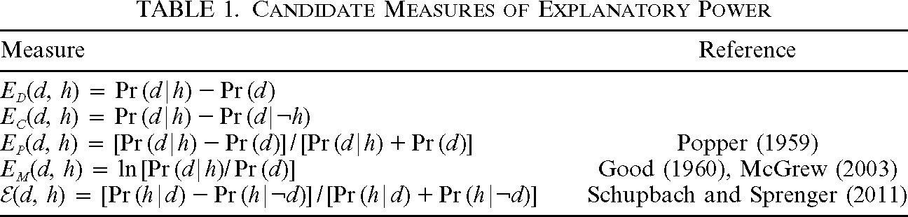
 . This project was undertaken decades ago by Popper (Reference Popper1959) and Good (Reference Good1960, Reference Good1968). Very recently, McGrew (Reference McGrew2003) and Schupbach and Sprenger (Reference Schupbach and Sprenger2011) put forward such measures in their work. All of these corresponding measures, along with some other plausible candidate measures, are shown in table 1.

| Measure | Reference |
 |
|
 |
|
 |
Popper (Reference Popper1959) |
 |
Good (Reference Good1960), McGrew (Reference McGrew2003) |
 |
Schupbach and Sprenger (Reference Schupbach and Sprenger2011) |
Measures  and
 are both related to Bayesian measures of confirmation; in fact, these measures are structurally equivalent to the confirmation measures of Keynes (Reference Keynes1921) and Kemeny and Oppenheim (Reference Kemeny and Oppenheim1952). However, regarding interpretation, each reference to evidence
 and hypothesis
 in the confirmation measures is replaced with a reference to
 and
 , respectively, in these measures. Measures
 and
 have been built in the same way from two other confirmation measures—due to Eells (Reference Eells1982) and Christensen (Reference Christensen1999), respectively—and added to the list of measures to consider here.
It is also worth noting that  and
 are closely related. Indeed, they are ordinally equivalent to one another, meaning that they always impose the same ordinal relations on degrees of explanatory power. Put formally, for any
 ,
 ,
 , and
 ,
 =,
 if and only if
 =,
 .
Each of the measures shown in table 1 aims to clarify the precise formal relation that is attained between  and
 to the extent that the former is explanatory of the latter. It has been argued that these measures thereby allow us to answer substantive questions about the epistemic value of explanatory power. In fact, all three of the above measures that have been put forward in the literature have been used to defend explanatory reasoning as having normative merit. McGrew (Reference McGrew2003, 558), for instance, shows (in terms of his measure
 ) that “of two hypotheses with equal priors, the one with greater explanatory power will have the greater posterior probability”; Schupbach (Reference Schupbach2011, chap. 5) gives this same result in terms of
 . Similarly, Popper (Reference Popper1959, 401) proves that the amount of explanatory power (as measured by
 ) that a hypothesis has relative to some evidence is positively related to the degree of “corroboration” that the former receives from the latter.
These measures thus attempt to provide normative accounts of explanatory power and explanatory reasoning. First and foremost, they offer competing formal accounts of how we ought to think about the concept of explanatory power. Additionally, they each assert that, under certain conditions, explanatory considerations do guide us to hypotheses that are more probable (or better corroborated). Accordingly, they tell us that we ought to reason explanatorily under such conditions. These measures thus unquestionably have interesting normative interpretations and consequences.
What has not yet been investigated regarding these measures is the separate question of whether any of them are also descriptive of people's actual explanatory judgments. Of course, the normative nature of these measures does not imply their descriptive accuracy. It may well be that a measure makes precise the way people generally ought to think about explanatory power and that, if they think about it in this way, then they ought to reason in favor of better explanations, and it may simultaneously be true that people do not typically do as they epistemically ought. Alternatively, if some measure doubles as a good descriptor of people's explanatory judgments, then the normative implications of that measure suggest an interesting defense of actual explanatory reasoning. The issue then is whether people actually think about explanatory power in any of the ways that these epistemologists have said that they should.
This descriptive study also has important bearing for the normative accounts themselves. Here, the question is to what extent the measures resemble the concept of explanatory power as it is generally used. If all of the measures diverge widely from people's actual explanatory intuitions, then it may be that people do not understand explanatory power in the way that they should; however, it might more plausibly be the case that the measures just fail to capture in any substantive way the notion of explanatory power. Conversely, if any particular candidate measure fits well with such intuitions, then this provides some support for the general accuracy of that particular measure.
This article investigates the descriptive question. In light of the above, it should thus be of interest to both philosophers and psychologists interested in explanatory reasoning.
2. Experiment: Comparing the Descriptive Merits of the Measures
In this section, I summarize my own recent experimental research investigating the descriptive question. The overarching goal of this project was to test and compare the relative descriptive merits of the aforementioned candidate measures of explanatory power. To this end, I used an experimental design based closely on a chance setup previously applied by Phillips and Edwards (Reference Phillips and Edwards1966) and more recently by Tentori et al. (Reference Tentori, Crupi, Bonini and Osherson2007) in their comparison of various Bayesian measures of confirmation.
2.1. Materials and Procedure
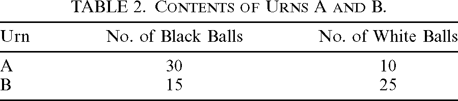
In this experiment, participants were asked to judge how well various hypotheses explain certain sets of data. These judgments were elicited during an individual interview involving a probabilistic scenario of black and white balls being drawn without replacement from one of two possible urns. During the interview, participants were first presented with two opaque urns and then informed of their respective contents. The urns were composed of black and white balls as specified in table 2. At this point, participants were also given a visual representation of the urns’ contents to which they could refer throughout the experiment.

| Urn | No. of Black Balls | No. of White Balls |
| A | 30 | 10 |
| B | 15 | 25 |
The decision of which urn to use throughout the remainder of the interview was next decided via an actual flip of a fair coin. Participants saw that the coin flip determined our choice of urn; however, whether the chosen urn was A or B was left hidden. The experiment then proceeded with a series of 10 random drawings without replacement from the chosen urn. These drawings and the corresponding results were performed in full view of the participants. Additionally, balls that were the results of prior drawings were lined in front of the participants in the order in which they had been withdrawn; thus, at any time during the interview, participants could refer to all of the results up to that point. Throughout each interview, the coin flip and drawings were truly chance events so that which urn was used and which balls were withdrawn differed between participants. Participants were faced with six tasks after each individual drawing.
Task 1. Participants were first asked to make a mark on an “impact scale” representing the degree to which “the hypothesis that urn A was chosen [( )] explains the results from all of the drawings so far.” Each impact scale was printed on a strip of paper and consisted of a dotted line with arrows pointing out of either end. The following five descriptive labels were spaced evenly from left to right over the line (with the line extending in both directions beyond the labels):
• This hypothesis is an extremely poor explanation of the results collected so far.
• This hypothesis is a poor explanation of the results collected so far.
• This hypothesis is neither a good nor a poor explanation of the results collected so far.
• This hypothesis is a good explanation of the results collected so far.
• This hypothesis is an extremely good explanation of the results collected so far.
Fresh copies of the scale were used for each of the 10 drawings, and all of a participant's previously marked judgments were organized in his or her view to refer to if desired. On a given impact scale, the marked distance from the neutral point was used to quantify judged degrees of explanatory power. Upon receiving the impact scale, participants were told that the scale was intended to be continuous and that distances would matter to how their responses were recorded.
Task 2. Next, participants were asked to repeat the first task but this time with regard to the hypothesis that urn B was chosen ( ). Ultimately then, participants were asked to make 20 judgments of explanatory power throughout the experiment (10 pertaining to
 and 10 pertaining to
 ).
Tasks 3 and 4. In tasks 3–6, participants estimated various relevant probabilities. For the first two of these tasks, participants were faced with the following two questions (in the questions listed below,  was set to the number of balls that had been drawn at that point in the interview):
• Considering the color of the first
 balls, what now is the probability that the urn selected is A?
• Considering the color of the first
balls, what now is the probability that the urn selected is B?
 balls, what now is the probability that the urn selected is A?
 balls, what now is the probability that the urn selected is B?
Participants were instructed that their answers could be written in whatever format they preferred (decimals, fractions, or percentages); however, they had to sum either to 1 (if they chose to write decimals or fractions) or 100%.
Tasks 5 and 6. For the final two tasks performed with each drawing, participants were asked the following two questions:
• Assuming that the selected urn is A, what at this point was the probability of drawing a ball of this color?
• Assuming that the selected urn is B, what at this point was the probability of drawing a ball of this color?
Again, participants were instructed that their answers could be written in whatever format they preferred; for these two questions, it was pointed out that there was no need for the two answers to sum to 1 (or 100%).
Tasks 3 and 4 were used to assess participants’ judgments about the probabilities of the respective hypotheses conditional on all of the “evidence” received from the drawings. That is, in the  th round of the interview, each participant's response to task 3 was interpreted as that person's subjective probability for
 conditional on the
 results of all of the drawings up to that point:
 . Similarly, participants’ responses to task 4 were taken to provide values for
 .
On the other hand, tasks 5 and 6 assessed participant judgments about the probabilities of the latest result conditional on the respective hypotheses and all preceding results. That is, in the  th round of the interview, each participant's response to task 5 was interpreted as that person's subjective probability for the result of the
 th drawing conditional on
 and on the
 preceding results:
 . Similarly, responses to task 6 were taken to provide values for
 .
Given the chance nature and the quantitative details of this experimental design, the following corresponding objective probabilities were calculated for each drawing in each interview:  ,
 ,
 , and
 . These probabilities (in both their subjective and objective varieties) were then plugged into the measures listed in table 1 in order to derive theoretical degrees of explanatory power for
 and
 . In this way, the experiment elicited a host of participant judgments about explanatory power along with the same number of corresponding results derived from each measure (first using subjective probabilities and then using objective probabilities).
2.2. Participants
Twenty-six undergraduate students from the University of Pittsburgh participated in this study in exchange for $10 each. The average age of the participants was 20 years. Among the participants, there were 14 men and 12 women.
3. Results
3.1. Preparing the Measures for Comparison
To compare the descriptive accuracies of the measures, we rely first on the measure of the Euclidean distance between participant judgments and the “theoretical results” derived from each particular measure. This distance (relative to a particular hypothesis  , and in
 -dimensional space) between a set of
 judged degrees of explanatory power and a corresponding set of
 theoretical results is given by the following equation, where
 represents a participant's judgment of the degree to which
 explains
 , and
 stands in for any particular candidate measure of explanatory power:

In words, the Euclidean distance  between participant judgments
 and the theoretical results derived from E is given by summing the squares of the “residuals” (the differences between each judged value and theoretical value) and then calculating that sum's square root. The lower the value of
 , the closer E is to participant judgments J.
This choice of measure requires defense, especially in light of Tentori et al.'s similar study comparing the descriptive merits of various confirmation measures. Tentori et al. (Reference Tentori, Crupi, Bonini and Osherson2007, 115) rely primarily on a Pearson correlation test to decide which confirmation measure “corresponds most closely to judged evidential impact.” The experimental design applied here is based on that used by Tentori et al.; furthermore, the nature of our experimental results and our aims in analyzing them are closely related. So why is there this change in how we proceed with the analysis?
Pearson's correlation test measures the degree of linear dependence that holds between two variables. As such, it provides a powerful tool for showing the degree to which the values of one variable can be predicted as a linear function of another variable. More specific to our context, if J and a set of theoretical results derived from a measure E were shown to be highly correlated, then this would constitute evidence that E could be used as a predictor of people's explanatory judgments. This would surely be an interesting finding. However, a measure of explanatory power that hopes to be descriptively valid claims to be more than merely capable of being made into a good predictor of such judgments. Indeed, the most descriptively accurate measure will be the one whose results actually correspond most closely to judged degrees of explanatory power themselves. This notion of proximity is just what is measured by a distance measure such as d. On the other hand, the concept of correlation can diverge significantly from this notion. Indeed, two variables can be perfectly correlated even while taking vastly different corresponding values. Thus, in order to test the full descriptive merits of our measures, we opt for a distance measure.Footnote 1
Our choice to use a distance measure does, however, lead to a new complication. In order for us to compare the distances between each of our measures and actual human judgments, all derived and judged degrees of explanatory power must be identically scaled. Participants’ marked judgments are easily placed onto a [−1, 1] scale with the extreme left point of the dotted line on the impact scale representing −1, the center point 0, and the extreme right point 1. Moreover,  ,
 ,
 , and
 are all on the same [−1, 1] scale with interpretations corresponding to the labels provided with the impact scale. Measure
 agrees with our other candidate measures that the value 0 is to be interpreted as the neutral point at which
 is “explanatorily irrelevant” to d. However, while all other candidate measures are finitely scaled,
 has the range
 . In order to measure the distance between the results provided by such a measure and a set of judged degrees on a finite scale then,
 must be given a finite rescaling.
This can be done by feeding the results of  into any function that has all of the real numbers as its domain and the real numbers from −1 to 1 as its range. More specifically, such a function minimally ought to satisfy the following conditions of adequacy in order to rescale
 appropriately:
Finite Boundedness. The function F must have all of the real numbers as its domain and the set of real numbers from −1 to 1 as its range:
.Monotonicity. F must be monotonically increasing:
.Neutrality.
if and only if .Asymptotic Behavior. The rate at which
increases or decreases approaches 0 for the limiting points: and .
 .
 .
 if and only if
 .
 increases or decreases approaches 0 for the limiting points:
 and
 .
These conditions of adequacy are all easily motivated as requirements for our function F. Finite Boundeness has already been discussed above. Monotonicity ensures that the degree of explanatory power as measured by F will increase with the degree of explanatory power as measured by  . We also want F to preserve the fact that
 is normalized around 0 with this value representing explanatory irrelevance; thus, we require Neutrality. Finally, as values of
 increase (or decrease) without bound, corresponding degrees of explanatory power become less distinguishable and their differences less meaningful. Accordingly, we enforce the Asymptotic Behavior requirement for F.
Hartmann and Sprenger (Reference Hartmann and Sprenger2010) introduce (for purposes entirely different than our own) a family of functions that, with a minor modification elegantly satisfies our conditions of adequacy.Footnote 2 This family is defined by the following equation:

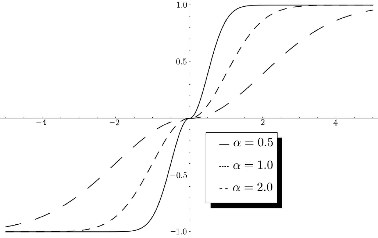
Here  provides us with any number of functional rescalings of
 depending on the parameter α (three members of the
 family are pictured in fig. 1). This fact constitutes a significant advantage for
 when it comes to testing and comparing our measures’ proximities to participant judgments. To measure
 's distance from participant judgments, we can essentially evaluate a wide range of the members of
 and then choose that member of
 that is closest. In this sense,
 is much more flexible and thereby has a prima facie advantage over the other measures.
Three members of the  family.

3.2. Comparing the Measures
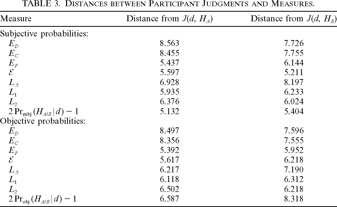
We are now prepared to compare the descriptive merits of our various candidate measures of explanatory power. Results are displayed in the top half of table 3. We first apply measure  to the results derived from each of our candidate measures of explanatory power using participants’ subjective probabilities. These results change somewhat if we now apply the measure
 to the results derived from the candidate measures using objective probabilities. Results are displayed in the bottom half of table 3.

| Measure | Distance from  |
Distance from  |
| Subjective probabilities: | ||
 |
8.563 | 7.726 |
 |
8.455 | 7.755 |
 |
5.437 | 6.144 |
 |
5.597 | 5.211 |
 |
6.928 | 8.197 |
 |
5.935 | 6.233 |
 |
6.376 | 6.024 |
 |
5.132 | 5.404 |
| Objective probabilities: | ||
 |
8.497 | 7.596 |
 |
8.356 | 7.555 |
 |
5.392 | 5.952 |
 |
5.617 | 6.218 |
 |
6.217 | 7.190 |
 |
6.118 | 6.312 |
 |
6.502 | 6.218 |
 |
6.587 | 8.318 |
This table reveals some interesting findings. First, the last row of the top and bottom half of each table provides the distance between participant judgments and the corresponding posterior probabilities (rescaled to [−1, 1]) that the urn chosen is A or is B in light of d. These probabilities come remarkably close to participant judgments of explanatory power. In particular, the subjective posterior probabilities come closest to participant judgments about  , while these probabilities are second only to
 in proximity to judgments about
 . These results might suggest either of the following. First, it could be that participants confuse the concepts of explanatory power and probability; in this case, when asked to judge how well a hypothesis explains some set of data, participants tend to read the question as asking for their judgment of how probable the hypothesis is in light of that data. Alternatively, participants may have distinct concepts of explanatory power and posterior probability that are nevertheless closely related (as the normative implications of our candidate measures would imply). In either case, we would expect participant judgments of one of these concepts to track judgments of the other. We will have more to say below about the relative merits of these two alternatives.
Second, the table shows that, whether we use subjective or objective probabilities in our derivations, measures  ,
 , and various rescalings of
 consistently come the closest of all of the measures to participant judgments. This observation immediately leads to a further question insofar as we want a full comparison of our measures. Recall that measure
 has the advantage of corresponding to any number of rescaled measures
 . While
 and
 look as though they generally come closer to participant judgments than
 ,
 , or
 , it may be that some other rescaling of
 nonetheless outperforms
 and
 . To investigate this possibility, we must run a more careful analysis of the
 family to get a closer estimate of which of its members comes the closest to participant judgments. Then, we can compare that member to
 and
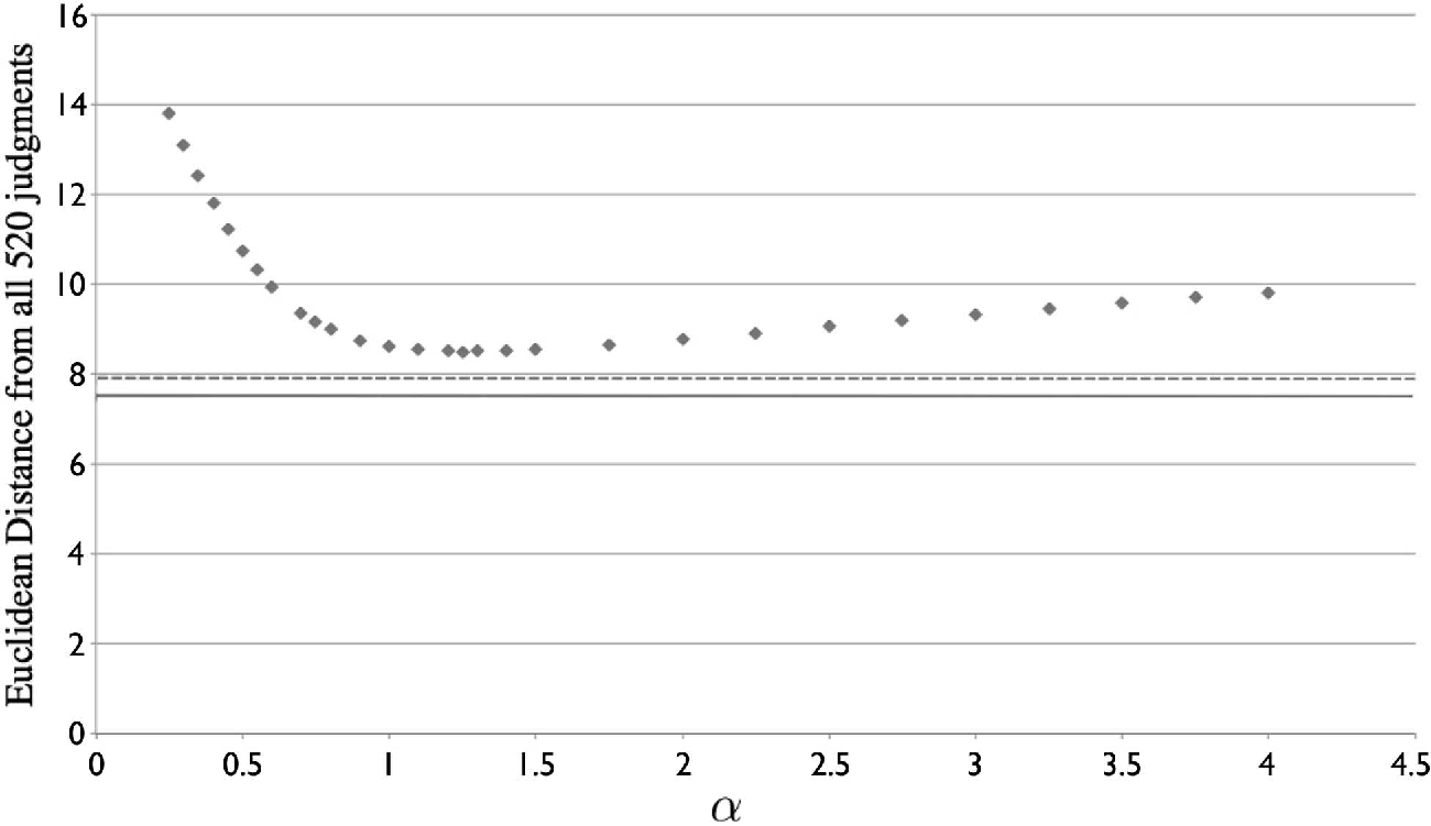
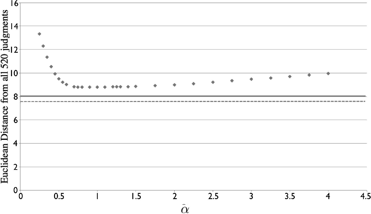
 . Figures 2 and 3 summarize the results of such an analysis. Looking at these figures, we can see that the overall Euclidean distance (over all 520 participant judgments—260 pertaining to
 and 260 pertaining to
 ) corresponding to members of
 never dips below that for
 or for
 . We can also now estimate which member of the
 family is the closest competitor to
 and
 . When using subjective probabilities, we estimate the best-performing member of
 to be
 ; when using objective probabilities, we choose
 .
Distances of members of  (dots) versus those of
 (dashed line) and
 (solid line) calculated using subjective probabilities.

Distances of members of  (dots) versus those of
 (dashed line) and
 (solid line) calculated using objective probabilities.

In light of the preceding discussion, at least two important questions still remain. First, do participants simply conflate the notions of explanatory power and posterior probability, or do they take these to be distinct, albeit closely related to one another? Second,  and
 are generally shown by d to be closer to participant judgments than the other measures. Yet one might still wonder what degree of confidence we can have in this conclusion given our data and whether we can run a distinct comparison between these two measures which will single one out as providing the best fit with participants’ judgments.
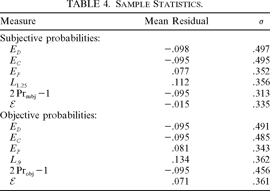
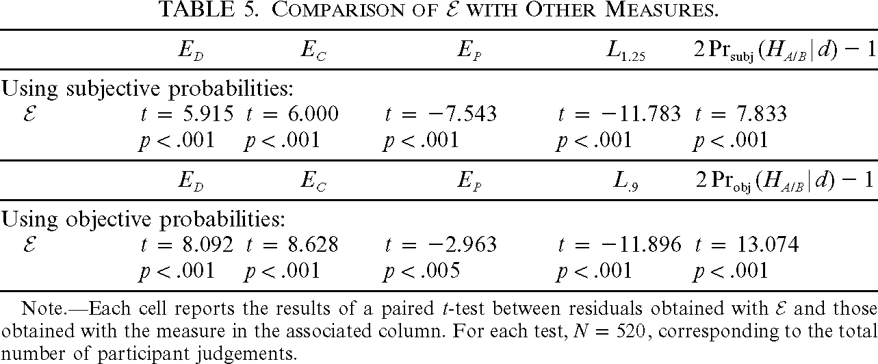
As it turns out, we can shed light on both of these questions by performing a more sophisticated comparison of our measures. Specifically, we compare the various distributions of the residuals (i.e.,  ) between the theoretical results provided by each candidate measure and participant judgments. Mean residuals (and corresponding standard deviations) are displayed in table 4. As this table shows,
 's results have the mean residual that comes closest to the ideal value of 0, and this is true whether we are using subjective or objective probabilities to derive our theoretical values. Furthermore, table 5 reveals results from a series of paired t-tests collectively showing that
 's mean residual differs quite significantly from each of those corresponding to the other measures. Note, in particular, that
 's mean residual is significantly closer to 0 than that of
 and
 (when using subjective probabilities) and
 and
 (when using objective probabilities). Accordingly, from our experimental data, we can now conclude that
 comes significantly closer to participant judgments than any other candidate measure (including any
 rescaling of
 ).

| Measure | Mean Residual |  |
| Subjective probabilities: | ||
 |
−.098 | .497 |
 |
−.095 | .495 |
 |
.077 | .352 |
 |
.112 | .356 |
 |
−.095 | .313 |
 |
−.015 | .335 |
| Objective probabilities: | ||
 |
−.095 | .491 |
 |
−.095 | .485 |
 |
.081 | .343 |
 |
.134 | .362 |
 |
−.095 | .456 |
 |
.071 | .361 |

 |
 |
 |
 |
 |
|
| Using subjective probabilities: | |||||
 |
 |
 |
 |
 |
 |
 |
 |
 |
 |
 |
|
 |
 |
 |
 |
 |
|
| Using objective probabilities: | |||||
 |
 |
 |
 |
 |
 |
 |
 |
 |
 |
 |
|
Note Each cell reports the results of a paired t-test between residuals obtained with  and those obtained with the measure in the associated column. For each test,
 , corresponding to the total number of participant judgements.
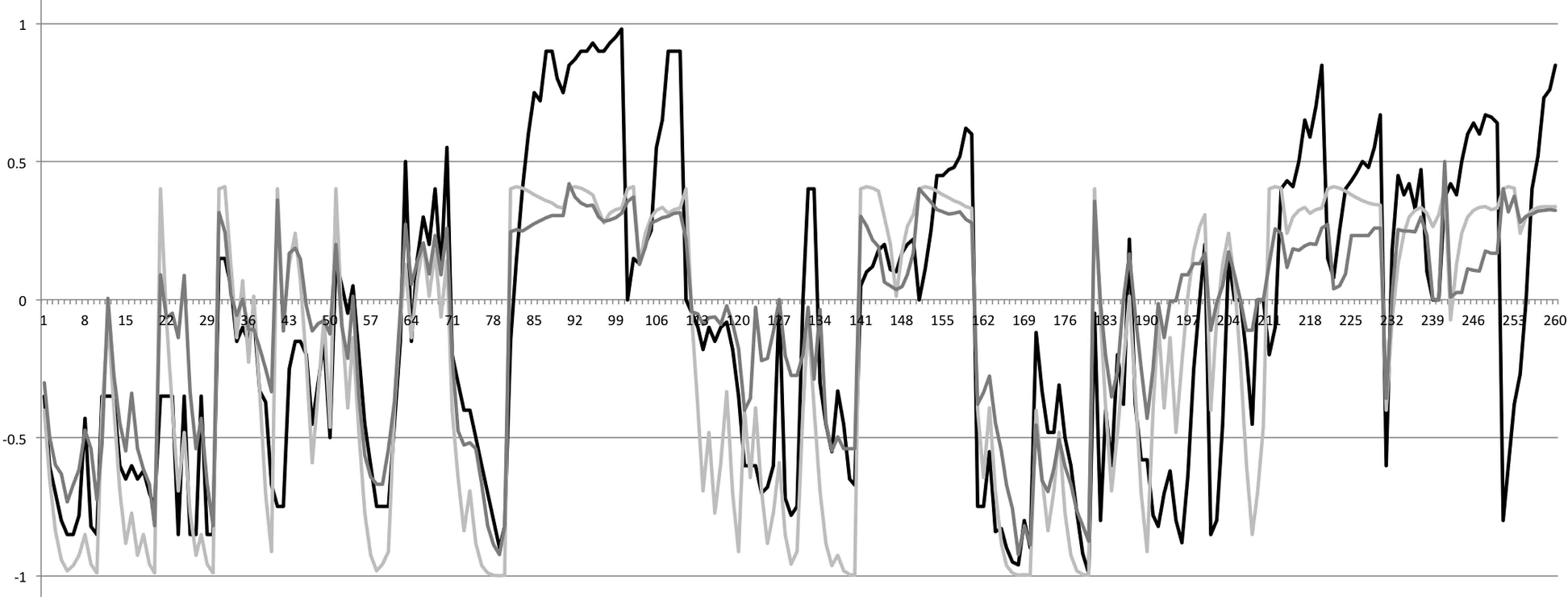
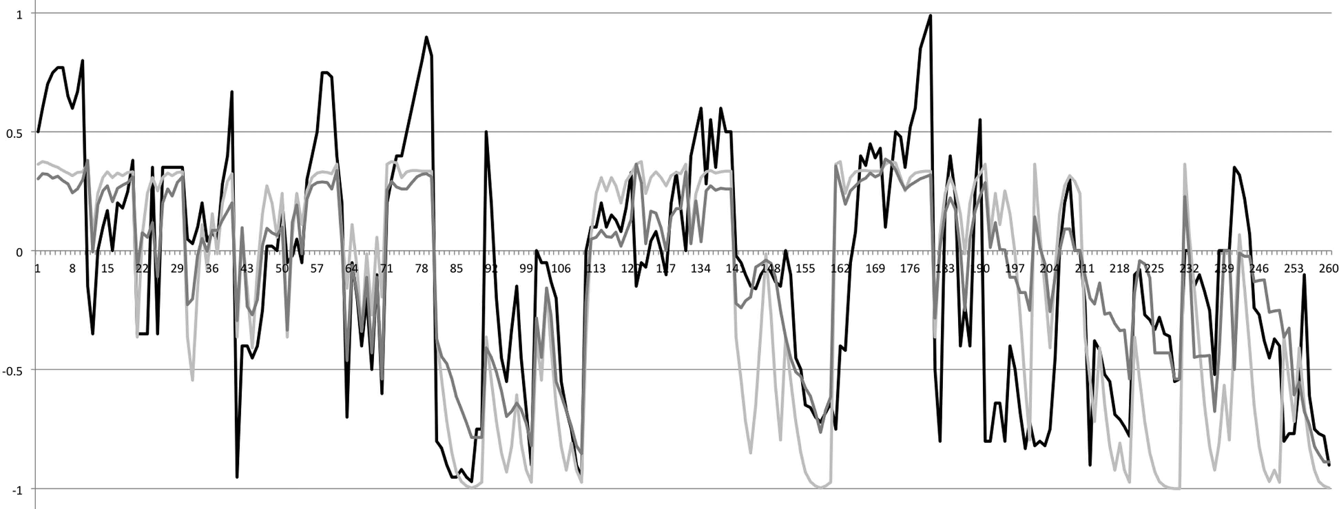
Importantly,  not only does comparatively well in this regard, but it also does remarkably well on its own. In particular, the mean residual between
 's results (calculated using subjective probabilities) and participant judgments does not differ significantly from
 (
 ,
 ,
 ). This result does not hold true for any other measure; in all other cases (using either subjective or objective probabilities) a measure's mean residual differs significantly from the ideal value
 (for all of these comparisons,
 ). Figures 4 and 5 give visual representations of the fit between
 and participant judgments.
Participant judgments about  (black) plotted with values derived from
 using subjective probabilities (dark gray) and objective probabilities (light gray).

Participant judgments about  (black) plotted with values derived from
 using subjective probabilities (dark gray) and objective probabilities (light gray).

We may now return to the question of whether participants are simply conflating the notions of explanatory power and posterior probability. If this were true, then we would expect the mean residual corresponding to the posterior probability to be very close to 0. This should particularly prove true in cases in which the residuals represent the differences in a participant's judged degree of explanatory power and that same participant's own stated subjective posterior probability; presumably, a participant who conflates these two concepts will give the same response in each case. In the subjective and objective cases, however, the mean residual is −.095, which differs very significantly from the expected value of 0 ( using subjective probabilities, and
 using objective probabilities). This means that, on average (over 520 data points), participants judge explanatory power to be significantly lower than the corresponding posterior probability. Thus, our experimental data provide us with evidence that, even while intuitions about explanatory power are linked closely to judgments of posterior probability (as evidenced by their small Euclidean distance), these notions remain conceptually distinct.
4. Discussion
This experiment has important implications for both the epistemology and the psychology of explanatory reasoning. Regarding the former, Schupbach and Sprenger (Reference Schupbach and Sprenger2011) argue that measure  corresponds most closely to our notion of explanatory power because this measure alone satisfies several intuitive conditions of adequacy for such an account. This article augments that case for
 with empirical evidence suggesting that this measure also does the best at describing actual explanatory judgments. The case for
 as our most accurate formal analysis of explanatory power thus looks to be strong indeed.
Regarding this experiment's implications for psychology, the results here support the claim that  is a useful predictor of human explanatory judgments. At worst then,
 provides psychologists with a useful but merely instrumental theory of explanatory reasoning. On the other hand, at best,
 may lend insight into some of the mental heuristics—and ultimately the cognitive mechanisms—that people use in making judgments pertaining to explanation and probability. To take one example, from these experiments, we see clear signs that participants’ judgments of explanatory power are closely aligned with, though distinct from, their judgments of probability. This finding accords well with the normative implications of
 , as spelled out in Schupbach (Reference Schupbach2011). It also suggests that people may well use their intuitions about how well a hypothesis explains data as a heuristic when trying to gauge that hypothesis's probability in light of those data. As Peter Lipton (Reference Lipton2004, 121) repeatedly quips: “explanatory loveliness is a guide to judgments of likeliness.”
Last, and of interest to both philosophers and psychologists, these experiments form the basis of a normative defense of everyday human explanatory reasoning. If, as suggested here, people's explanatory judgments fit well with the formal account  , then their judgments will tend to benefit from this measure's positive, normative implications. Consequently, given that, according to
 , the best explanation of some set of facts d must also be the most probable hypothesis in light of d (under certain formal conditions), and given that people's explanatory judgments tend to agree with the results of
 , then (given certain corresponding conditions) people will tend to choose more probable hypotheses when they reason explanatorily. The specific conditions that must attain in order for this to hold true can be spelled out quite precisely (thanks to the clarity inherent in the formal analysis
 ). Such further work, moreover, can give us a better sense of where we should expect explanatory reasoning to break down and lead humans astray given
 . Such a project is beyond the scope of the current article, however, and thus constitutes one possible avenue for further research in the light of this study.

 , which satisfies Monotonicity only in the domain
 . Our measure
 provides us with a function that satisfies Monotonicity generally over
 .