





1. Introduction
Slippery surfaces, including superhydrophobic (SH) surfaces, have received much attention in recent years since they provide a drag reduction and flow manipulation in microfluidic devices (Rahmani et al. Reference Rahmani, Larachi and Taghavi2024; Bai et al. Reference Bai, Zhao and Cao2025). The SH surfaces constitute a particularly notable category, distinguished by a combination of microscale/nanoscale roughness and low surface energy, often achieved through hydrophobic coatings or surface chemical modification, which facilitates air entrapment within their structured features (Gaddam et al. Reference Gaddam, Sharma, Ahuja, Dimov, Joshi and Agrawal2021; Khan & Daschakraborty Reference Khan and Daschakraborty2024). The presence of this air layer serves to markedly diminish friction at the interface, thereby amplifying slip effects and significantly reducing drag (Gluzdov & Gatapova Reference Gluzdov and Gatapova2023; Xu et al. Reference Xu, Ruan and Zhang2024). Nevertheless, the realization of large slip lengths in practical systems can be strongly compromised by trace surfactants or interfacial contaminants, which may generate Marangoni stresses and partially immobilize the liquid–air interface, thereby reducing the expected drag-reduction performance (Peaudecerf et al. Reference Peaudecerf, Landel, Goldstein and Luzzatto-Fegiz2017). Owing to these remarkable attributes, SH surfaces have garnered significant attention in the study of microfluidic systems (Yohe et al. Reference Yohe, Colson and Grinstaff2012; Falde et al. Reference Falde, Freedman, Herrera, Yohe, Colson and Grinstaff2015; Seo et al. Reference Seo, García-Mayoral and Mani2018) and fluid transport phenomena (Ijaola et al. Reference Ijaola, Farayibi and Asmatulu2020; Hasan et al. Reference Hasan, Sun, Bahaeddine, Liang, Damulira and Chen2024).
Seminal studies by Philip (Reference Philip1972a , Reference Philipb ) established the classical framework for Newtonian flow over surfaces combining no-slip and no-shear regions, forming the basis for slip analysis on patterned substrates. Lauga & Stone (Reference Lauga and Stone2003) subsequently derived semianalytical solutions for pressure-driven flows under such mixed boundary conditions. Building on this foundation, numerous works (Feuillebois et al. Reference Feuillebois, Bazant and Vinogradova2009, Reference Feuillebois, Bazant and Vinogradova2010; Belyaev & Vinogradova Reference Belyaev and Vinogradova2010; Vinogradova & Belyaev Reference Vinogradova and Belyaev2011; Schmieschek et al. Reference Schmieschek, Belyaev, Harting and Vinogradova2012; Zhou et al. Reference Zhou, Belyaev, Schmid and Vinogradova2012; Asmolov et al. Reference Asmolov, Zhou, Schmid and Vinogradova2013; Nizkaya et al. Reference Nizkaya, Asmolov and Vinogradova2013; Dubov et al. Reference Dubov, Nizkaya, Asmolov and Vinogradova2018; Asmolov et al. Reference Asmolov, Nizkaya and Vinogradova2020) systematically quantified effective slip lengths for creeping flows over SH surfaces with varying groove geometries and periodic textures. Complementary analytical treatments (Crowdy Reference Crowdy2010; Crowdy Reference Crowdy2016, Reference Crowdy2017b,c , Reference Crowdy2021; Kirk et al. Reference Kirk, Karamanis, Crowdy and Hodes2020; Mayer & Crowdy Reference Mayer and Crowdy2022; Miyoshi et al. Reference Miyoshi, Rodriguez-Broadbent, Curran and Crowdy2022; Rodriguez-Broadbent et al. Reference Rodriguez-Broadbent, Miyoshi and Crowdy2024) examined longitudinal and transverse grooves, clarifying the roles of symmetry, interfacial curvature and boundary-condition arrangement. Related studies (Hodes et al. Reference Hodes, Kirk, Karamanis and MacLachlan2017; Kirk et al. Reference Kirk, Hodes and Papageorgiou2017; Kirk et al. Reference Kirk, Karamanis, Crowdy and Hodes2020; Hodes et al. Reference Hodes, Kane, Bazant and Kirk2023) addressed pressure-driven and thermocapillary flows, highlighting velocity-field asymmetries and flow–geometry coupling. These studies established the fundamental understanding of slip mechanisms, interface morphology and geometric confinement in creeping Newtonian flows. It should be emphasized, however, that the Stokes-flow limit adopted in these classical analyses does not necessarily restrict effective-slip descriptions to Reynolds numbers much smaller than unity. In laminar flows over some SH textures, especially ridges or grooves aligned with the mean flow direction (i.e. nearly parallel flows), the effective slip may remain only weakly dependent on the Reynolds number over a finite Reynolds number range (Cheng et al. Reference Cheng, Teo and Khoo2009). Such behaviour is, however, geometry- and regime-dependent, since secondary effects associated with flow-induced meniscus deformation, gradients in meniscus curvature or variations in the liquid and gas cross-sectional areas may introduce finite-Reynolds-number corrections (Hyväluoma & Harting Reference Hyväluoma and Harting2008; Gao & Feng Reference Gao and Feng2009; Asmolov et al. Reference Asmolov, Nizkaya and Vinogradova2020).
More recent work has extended this framework to increasingly realistic regimes. Numerical studies incorporating inertia, microchannel confinement and structured surfaces with posts, holes or longitudinal slits (Game et al. Reference Game, Hodes, Keaveny and Papageorgiou2017; Sharma et al. Reference Sharma, Gaddam, Agrawal, Joshi and Dimov2019, Reference Smith, Varanasi, Jordan and Boers2020; Zimmermann & Schönecker Reference Zimmermann and Schönecker2024) demonstrated departures from classical creeping-flow scaling. For longitudinal ridges, Game et al. (Reference Game, Hodes and Papageorgiou2019) considered pressure-driven flow in the Cassie state when the meniscus curvature varies slowly along the channel. Their asymptotic analysis showed that such axial variations lead to a non-parallel flow and modify the relation between flow rate and pressure drop, thereby introducing inertial corrections beyond the usual fully developed slip description. In a related finite-Reynolds-number context, Cowley et al. (Reference Cowley, Maynes and Crockett2016) numerically studied laminar SH microchannel flow and proposed empirical correlations in which the apparent slip length depends on both Reynolds number and texture geometry. Moreover, Sharma et al. (Reference Sharma, Gaddam, Agrawal and Joshi2019) showed that effective slip depends on Reynolds number, viscosity contrast and cavity aspect ratio, while Zimmermann & Schönecker (Reference Zimmermann and Schönecker2024) quantified the combined effects of groove morphology and viscosity variation for circular grooves and longitudinal slits. Experimental investigations have further refined this picture: Ko et al. (Reference Ko, Kim, Ha and Lee2020) reported large slip lengths
 $(\sim 8\,{\unicode[Arial]{x03BC}} \mathrm{m})$
and strong air retention for copper oxide nanostructures, and Ren et al. (Reference Ren, Chen, Mu, Khoo, Zhang and Xu2018, Reference Ren, Hu, Bao, Zhang, Wen and Xie2021) demonstrated how inertia modifies drag reduction and slip behaviour, bridging classical theory and practical microfluidic conditions.
Despite extensive work on Newtonian flows over SH surfaces, non-Newtonian counterparts remain comparatively underexplored (Rahmani et al. Reference Rahmani, Larachi and Taghavi2024). Existing studies have largely focused on shear-thinning fluids (Haase et al. Reference Haase, Wood, Sprakel and Lammertink2017; Patlazhan & Vagner Reference Patlazhan and Vagner2017; Gaddam et al. Reference Gaddam, Sharma, Ahuja, Dimov, Joshi and Agrawal2021; Ray et al. Reference Ray, Bouvier and Papageorgiou2023). For example, Crowdy (Reference Crowdy2017a ) analysed semi-infinite shear-driven flows over SH surfaces with longitudinal and transverse grooves, showing that shear-thinning rheology enhances effective slip relative to Newtonian fluids. In pressure-driven configurations, Haase et al. (Reference Haase, Wood, Sprakel and Lammertink2017) reported a non-monotonic dependence of slip length on flow velocity for transverse SH textures. Complementary experimental and numerical work by Gaddam et al. (Reference Gaddam, Sharma, Ahuja, Dimov, Joshi and Agrawal2021) demonstrated that groove orientation and surface architecture strongly govern the flow response: as in Newtonian systems, slip is substantially larger over longitudinal grooves and post arrays than over transverse grooves or perforated surfaces. By contrast, shear-thickening rheology suppresses interfacial slip, leading to reduced slip lengths compared with Newtonian behaviour (Zhang et al. Reference Zhang, Zhou, Crick, Ng and Poole2025).
Viscoplastic fluids, on the other hand, behave differently due to the presence of a yield stress, below which they behave as a solid and above which they flow. This behaviour leads to the formation of a plug layer at the liquid–air interface, referred to as the SH plug (Rahmani & Taghavi Reference Rahmani and Taghavi2022, Reference Rahmani and Taghavi2023). Consequently, the effective slip length over SH surfaces in viscoplastic fluids is strongly governed by the yield stress (Rahmani & Taghavi Reference Rahmani and Taghavi2022, Reference Rahmani and Taghavi2023). Beyond the SH plug, viscoplastic fluids can also develop a central plug region within the bulk flow (Frigaard et al. Reference Frigaard, Howison and Sobey1994; Rahmani & Taghavi Reference Rahmani and Taghavi2022). The morphology of this centre plug is influenced by various parameters, including the yield stress, flow rate and the characteristics of SH surface’s grooves (Rahmani & Taghavi Reference Rahmani and Taghavi2022, Reference Rahmani and Taghavi2023; Rahmani et al. Reference Rahmani, Kumar, Greener and Taghavi2023; Rahmani & Taghavi Reference Rahmani and Taghavi2024b ). Recently, it was demonstrated that, in thin channels, the unyielded central plug can undergo significant deformation and, at high slip numbers, may even break. Conversely, in thick channels, the unyielded plug largely retains its shape, characterized by a flat yield surface (Rahmani & Taghavi Reference Rahmani and Taghavi2022, Reference Rahmani and Taghavi2023; Rahmani et al. Reference Rahmani, Kumar, Greener and Taghavi2023; Rahmani & Taghavi Reference Rahmani and Taghavi2024a , Reference Rahmani and Taghavib ). Notably, the presence of two SH walls not only enhances the effective slip length, reducing drag substantially, but also affects the morphology of the central unyielded plug (Joulaei et al. Reference Joulaei, Rahmani and Taghavi2024). The relative alignment or misalignment of grooves on the opposing walls plays an important role in determining the morphology of the plug, its deformation or its breakage. To explore the optimal misalignment between two SH walls for achieving maximum velocity field asymmetry, deep learning techniques were employed. This optimal misalignment is influenced by both the yield stress and the groove characteristics (Joulaei et al. Reference Joulaei, Pal, Rahmani and Taghavi2025a ). Furthermore, introducing asymmetric groove morphology on the upper and lower SH surfaces defines the concept of slippery equivalent systems, where different groove configurations on the walls can produce identical effective slip lengths, but lead to distinct centre plug morphologies (Joulaei et al. Reference Joulaei, Rahmani and Taghavi2025b ).
To analyse the slip behaviour of SH surfaces with a given liquid–gas interface, many studies (including those mentioned above) have applied either shear-free (Luchini Reference Luchini2015; Kirk et al. Reference Kirk, Karamanis, Crowdy and Hodes2020) or partial-slip boundary conditions at the liquid–gas interface, often assuming it to be perfectly flat (Dubov et al. Reference Dubov, Nizkaya, Asmolov and Vinogradova2018; Bao et al. Reference Bao, Priezjev and Hu2020; Ren et al. Reference Ren, Hu, Bao, Zhang, Wen and Xie2021; Rahmani & Taghavi Reference Rahmani and Taghavi2022). In this idealized single-phase flow problems, both the meniscus curvature and dynamics of the gas phase are neglected. Some more recent investigations have explored the role of meniscus curvature in determining the frictional properties of SH surfaces, while considering single-phase flow problems (Crowdy Reference Crowdy2010, Reference Crowdy2016; Haase et al. Reference Haase, Wood, Sprakel and Lammertink2017; Li et al. Reference Li, Ji, Zhang and Li2023). Most of these studies neglected gas flow dynamics, focusing instead on the relationship between the meniscus protrusion angle and the effective slip length. In this regard, several studies (Haase et al. Reference Haase, Karatay, Tsai and Lammertink2013; Arun et al. Reference Arun, Dilip and Ranjith2021; Li et al. Reference Li, Ji, Zhang and Li2023) have extensively examined bubble mattresses characterized by varying protrusion angles to assess their influence on the effective slip length, conclusively demonstrating that the optimal enhancement in slip is attained when the protrusion angle resides within the approximate range of
 $0^\circ$
–
 $10^\circ$
. Nevertheless, a key limitation of these studies is their neglect of flow-induced meniscus deformation, i.e. they assume the interfacial shape remains static despite evolving under hydrodynamic forces. A comparative overview of the single-phase analysis of the Newtonian and non-Newtonian flow over SH surfaces is presented in tables 1 and 2, respectively.
Summary of representative single-phase Newtonian flow studies over SH surfaces, highlighting the considered geometries, key modelling assumptions and principal physical outputs.

Table 1. Long description
A table with four columns and eleven rows. The columns are labeled ‘References’, ‘Geometry’, ‘Main limitations’, and ‘Principal outputs’. Each row provides details of different studies. Row 1: References, Asmolov et al. (2013); Geometry, Grooved channel wall; Main limitations, Small local slip length; sharp-edge effects neglected; Principal outputs, Scaling laws for effective slip length. Row 2: References, Belyaev & Vinogradova (2010); Geometry, Striped channel wall; Main limitations, Flat liquid–gas interface; negligible inertia; Principal outputs, Analytical expression for effective slip length. Row 3: References, Schmieschek et al. (2012); Geometry, Grooved channel wall; Main limitations, Stokes flow; undeformed meniscus; Principal outputs, Anisotropic slip-length tensor. Row 4: References, Schönecker & Hardt (2013); Geometry, Single groove on plate; Main limitations, Lubrication approximation; shallow grooves; Principal outputs, Elliptic spatial distribution of local slip. Row 5: References, Nizkaya et al. (2014); Geometry, Single groove on plate; Main limitations, Large viscosity contrast limit; Principal outputs, Smooth effective slip profiles. Row 6: References, Davies et al. (2006); Geometry, Ribbed microchannel; Main limitations, Flat meniscus; Newtonian fluid; Principal outputs, Reduction in pressure drop. Row 7: References, Ou & Rothstein (2005); Geometry, Striped channel wall; Main limitations, Flat interface; Principal outputs, Experimental validation of slip velocity. Row 8: References, Teo & Khoo (2010); Geometry, Grooved channel wall; Main limitations, Longitudinal flow only; Principal outputs, Dependence of slip on meniscus curvature. Row 9: References, Ge et al. (2018); Geometry, Lubricant-filled groove; Main limitations, Two-phase Newtonian system; Principal outputs, Slip length and meniscus deformation versus Ca. Row 10: References, Hyväluoma & Harting (2008); Geometry, Bubble mattress; Main limitations, Deformable bubbles; moderate Ca; Principal outputs, Slip-length variation with bubble deformation. Row 11: References, Tomlinson & Papageorgiou (2022); Geometry, Grooved channel wall; Main limitations, Flat interface; linear stability analysis; Principal outputs, Identification of new instability modes.
Summary of representative single-phase non-Newtonian flow studies over SH surfaces, highlighting the considered geometries, key modelling assumptions and principal physical outputs.

Table 2. Long description
A table with four columns and nine rows. The columns are labeled ‘References’, ‘Geometry’, ‘Main limitations’, and ‘Principal outputs’. The rows list various studies with their respective geometries, main limitations, and principal outputs. Row 1: References, Crowdy (2017a); Geometry, Slotted flat plate; Main limitations, Weak shear-thinning; flat interface; Principal outputs, Perturbative correction to slip length. Row 2: References, Ray et al. (2023); Geometry, Grooved plate; Main limitations, Moderate meniscus deformation; longitudinal flow; Principal outputs, Non-monotonic dependence of slip on Carreau number. Row 3: References, Rahmani & Taghavi (2022); Geometry, Grooved channel wall; Main limitations, Mostly flat interface; limited inertia range; Principal outputs, Yielded and unyielded regions on the meniscus. Row 4: References, Patlazhan & Vagner (2017); Geometry, Grooved channel wall; Main limitations, Inelastic shear-thinning model; flat meniscus; Principal outputs, Apparent slip induced via theology. Row 5: References, Haase et al. (2017); Geometry, Bubble mattress; Main limitations, Two-dimensional transverse flow; Principal outputs, Slip enhancement due to shear-thinning effects. Row 6: References, Rahmani & Taghavi (2023); Geometry, Grooved channel wall; Main limitations, Thin-channel limit; regularized Bingham model; Principal outputs, Interaction between wall and core plug regions. Row 7: References, Rahmani et al. (2023); Geometry, Grooved channel wall; Main limitations, Flat-interface assumption; Principal outputs, Inertial effects on plug yielding. Row 8: References, Joulaei et al. (2024); Geometry, Grooved channel walls; Main limitations, Flat-interface assumption; Principal outputs, Groove misalignment between sidewalls affects the plug morphology. Row 9: References, Rahmani & Taghavi (2024a); Geometry, Patterned channel wall; Main limitations, Thick-channel limit; flat-interface assumption; Principal outputs, Longitudinal, transverse and oblique flow configurations. Row 10: References, Joulaei et al. (2025b); Geometry, Grooved channel with asymmetric SH walls; Main limitations, Flat-interface assumption; Principal outputs, Introduction of the slippery-equivalent system concept.
The dynamics of the liquid–air interface is a central determinant of SH surface performance and has been extensively investigated for Newtonian fluids. Analytical (Sbragaglia & Prosperetti Reference Sbragaglia and Prosperetti2007; Nizkaya et al. Reference Nizkaya, Asmolov and Vinogradova2014; Crowdy Reference Crowdy2016, Reference Crowdy2017b ; Asmolov et al. Reference Asmolov, Nizkaya and Vinogradova2020; Miyoshi et al. Reference Miyoshi, Rodriguez-Broadbent, Curran and Crowdy2022), numerical (Teo & Khoo Reference Teo and Khoo2010; Dubov et al. Reference Dubov, Nizkaya, Asmolov and Vinogradova2018; Ge et al. Reference Ge, Holmgren, Kronbichler, Brandt and Kreiss2018) and experimental (Karatay et al. Reference Karatay, Haase, Visser, Sun, Lohse, Tsai and Lammertink2013; Xue et al. Reference Xue, Lv, Liu, Shi, Lin and Duan2015; Mohammadshahi et al. Reference Mohammadshahi, Fanasia and Ling2025) studies have demonstrated that meniscus curvature strongly governs effective slip. In most works, interfacial protrusion or recession was controlled via hydrostatic pressure, while flow-induced deformation was largely neglected (Hyväluoma & Harting Reference Hyväluoma and Harting2008; Gao & Feng Reference Gao and Feng2009). Only a limited number of numerical studies addressed dynamic deformation, showing that strongly protruding, pinned bubbles undergo substantial shape changes at large capillary numbers, resulting in pronounced slip modification (Hyväluoma & Harting Reference Hyväluoma and Harting2008). Several studies further established that effective slip is highly sensitive to interface deflection (Biben & Joly Reference Biben and Joly2008; Li et al. Reference Li, Alame and Mahesh2017; Crowdy Reference Crowdy2017b ).
Semianalytical models accounting for trapped gas predicted a non-uniform distribution of local slip along the liquid–gas interface for Newtonian fluids (Schönecker & Hardt Reference Schönecker and Hardt2013; Nizkaya et al. Reference Nizkaya, Asmolov and Vinogradova2014; Schönecker et al. Reference Schönecker, Baier and Hardt2014), with the effective slip explicitly depending on the viscosities of both phases and the SH geometry (Schönecker et al. Reference Schönecker, Baier and Hardt2014). In shallow textures, the local slip length is governed by the viscosity contrast and the local gas-layer thickness (Nizkaya et al. Reference Nizkaya, Asmolov and Vinogradova2014; Dubov et al. Reference Dubov, Nizkaya, Asmolov and Vinogradova2018), whereas in deep textures it is controlled solely by the groove width and is independent of texture depth (Nizkaya et al. Reference Nizkaya, Asmolov and Vinogradova2014). Meniscus deformation may further lead to interface collapse: for transverse shallow grooves, the transition between deformed and collapsed states depends on capillary number, viscosity ratio and groove aspect ratio (Gao & Feng Reference Gao and Feng2009; Asmolov et al. Reference Asmolov, Nizkaya and Vinogradova2020). Interface failure may occur through depinning from groove edges, although for extremely shallow grooves the meniscus reaches the bottom wall before depinning can arise (Asmolov et al. Reference Asmolov, Nizkaya and Vinogradova2020). Depending on meniscus shape, distinct flow regimes emerge in which the interface remains pinned, depins or is entirely eliminated due to the competition between shear and surface tension (Gao & Feng Reference Gao and Feng2009), with the effective slip length intrinsically tied to the prevailing regime (Gao & Feng Reference Gao and Feng2009). More recent studies of partially filled and lubricant-infused SH grooves under transverse shear have shown that meniscus deformation and depinning depend sensitively on viscosity ratio, groove depth and the advancing contact angle of the outer liquid (Ge et al. Reference Ge, Holmgren, Kronbichler, Brandt and Kreiss2018; Asmolov et al. Reference Asmolov, Nizkaya and Vinogradova2020). A comparison of two-phase analyses for flow over SH surfaces is provided in table 3.
Representative two-phase flow studies over SH surfaces, summarizing the considered geometries, dominant modelling assumptions and principal physical outcomes related to slip and interfacial stability.

Table 3. Long description
The table has four columns: References, Geometry, Main limitations, and Principal outputs. It contains 18 rows, each representing a different study. Row 1: Vinogradova et al. (2009), Textured surfaces, Complex experimental protocols, Direct experimental measurement of slip. Row 2: Luchini (2015), Grooved surface, Shear-free liquid–gas interface, Assessment of effective-slip models. Row 3: Rothstein (2010), Patterned surface, Partial-slip boundary condition, Scaling of slip length with texture fraction. Row 4: Peaudecerf et al. (2017), Grooved channel, Surfactant-laden interfaces, Slip reduction via Marangoni stresses. Row 5: Bao et al. (2020), Microtextured surface, Flat liquid–gas interface, Drag reduction optimization. Row 6: Ren et al. (2021), Hierarchical texture, Undeformed meniscus, Multiscale textures. Row 7: Dubov et al. (2018), Grooved surface, Simplified gas-phase dynamics, Local slip boundary conditions. Row 8: Crowdy (2016, 2017b), Bubble mattresses, Inviscid gas assumption, Closed-form slip expressions for curved menisci. Row 9: Zhu et al. (2024), Microgrooved surface, Static contact-angle model, Influence of meniscus curvature on slip. Row 10: Li et al. (2023), Textured surface, Small-interface deformation, Spatial distribution of local slip. Row 11: Biben & Joly (2008), Grooved surface, Diffuse-interface formulation, Wetting and depinning dynamics. Row 12: Li et al. (2017), Micropillar array, Idealized pillar geometry, Interface deformation and drag trends. Row 13: Schönecker & Hardt (2013) and Schönecker et al. (2014), Grooved surface, Lubrication approximation, Non-uniform local slip profiles. Row 14: Nizkaya et al. (2014), Grooved surface, Stokes-flow regime, Gas-cushion model for effective slip. Row 15: Gao & Feng (2009), Grooved surface, Simple groove geometry, Interface collapse and failure regimes. Row 16: Asmolov et al. (2020), Grooved surface, Shallow grooves, Meniscus depinning and stability limits. Row 17: Joulaei et al. (2026a), Transverse grooved surface, Deep grooves; thin-channels limit, Design guideline for groove morphology.
While the influence of a deflected liquid–air interface on Newtonian fluid dynamics over SH surfaces has been extensively studied, the existing research on viscoplastic flows has predominantly assumed a flat interface. This assumption is restrictive for channel flows of yield-stress materials, such as Carbopol gels, emulsions, suspensions, cement pastes, drilling muds and coating or printing fluids, for which pressure-driven transport is controlled by the combined effects of wall slip, plug formation and local yielding (Geraud et al. Reference Geraud, Bocquet and Barentin2013; Younes et al. Reference Younes, Bertola, Castelain and Burghelea2020; Mollah et al. Reference Mollah, Poddar, Islam and Alam2021; Rahmani & Taghavi Reference Rahmani and Taghavi2026). In an SH channel, the liquid–air interface can therefore alter the flow not only by reducing friction, but also by changing the stress distribution that determines the SH plug and the yielded regions near the wall. Therefore, studying yield stress fluids over SH surfaces may provide insights into the possibility of drag reduction and flow control using superhydrophobicity for non-Newtonian fluids, which are generally associated with higher drag due to their larger apparent viscosities. The present work addresses this gap by analysing plane Poiseuille flow of a Bingham fluid in a channel with an air-filled grooved SH wall. Considering the superior performance of longitudinal grooves in drag reduction, an interesting topic for future work could be the study of yield stress Bingham fluids in channels decorated with longitudinal grooves. We employ a combined numerical and semianalytical approach. Our semianalytical framework tackles the two-phase problem by accounting for infinitesimal wall-induced perturbations, solving the governing equations via Fourier series expansion for the outer flow and a lubrication theory-based solution within the groove. This model is validated by complementary two-phase simulations in OpenFOAM, which also enable the analysis of a broader range of groove configurations where lubrication theory becomes inaccurate. Via these, we systematically investigate the problem across a wide spectrum of groove depths, quantifying the interplay between meniscus deformation and viscoplastic flow dynamics to provide a comprehensive and accurate framework for predicting flow behaviour over SH surfaces.
The present manuscript is organized as follows. Section 2 introduces the problem set-up and the governing equations, followed by descriptions of the numerical approaches and the semianalytical modelling in §§ 3 and 4, respectively. The main results are then discussed in § 6. Finally, § 7 provides a brief summary of the work and highlights the main conclusions.
2. Problem set-up and governing equations
2.1. Problem set-up
The present investigation examines Poiseuille flow of a viscoplastic fluid within a channel with a lower SH wall, characterized by transversely positioned air-filled grooves. The viscoplastic fluid flows from left to right, transverse to the groove direction. The air flow inside the groove resembles a two-dimensional cavity flow. The SH wall consists of a periodic array of rectangular grooves, showing a periodicity length of
 $\hat {L}$
, which, when normalized by the half-channel height
 $\hat {H}$
, defines the dimensionless periodicity length as
 $\ell = \hat {L}/\hat {H}$
. In the present study, we confine our analysis to a thick-channel regime, wherein
 $\ell \ll 1$
. The groove width and depth are denoted by
 $\hat {\delta }$
and
 $\hat {d}$
, respectively. We then define the slip area fraction on the SH surface as
 $\varphi = \hat {\delta }/\hat {L}$
, while the groove aspect ratio is expressed as
 $d = \hat {d}/\hat {\delta }$
(see figure 1).
The two-dimensional simulations are interpreted as representing the central region of a high-aspect-ratio microchannel, for which the width is much larger than the height and lateral-wall effects are negligible. Although finite-width channels may exhibit spanwise velocity variations and secondary circulations, these effects are expected to be negligible near the midwidth plane (Vagner & Patlazhan Reference Vagner and Patlazhan2019), where the flow approaches a two-dimensional Poiseuille-type state. A second modelling assumption concerns the streamwise periodicity of the textured wall. In a finite microchannel containing several SH grooves, as illustrated schematically in figure 1(a), inlet-induced disturbances may affect the first few texture periods. Once these entrance effects have decayed, however, the flow and the liquid–air interface response are expected to become nearly periodic over successive grooves, as commonly assumed in studies of patterned SH channels (Joulaei et al. Reference Joulaei, Rahmani and Taghavi2026a
). The present simulations therefore model this periodic region using a single representative groove with cyclic boundary condition in the streamwise direction, as shown in figure 1(b). The local meniscus geometry,
 $\hat {\eta }(\hat {x})$
, groove width and depth,
 $\hat {\delta }$
and
 $\hat {d}$
, and the interface and contact angles,
 $\theta$
and
 $\varTheta$
, are illustrated in figures 1(c) and 1(d). In figure 1(d) the schematic air flow inside the groove and the interfacial deformation associated with the onset of depinning are shown.
Three-dimensional schematic of viscoplastic flow in a channel with a lower SH surface. (b) Two-dimensional schematic of (a) is shown containing one groove, where axial velocity at the liquid–air interface is shown via pink colour. Velocity profile of yielded region (in black), centre plug velocity profile (in orange), liquid–air interfaces (in brown) and no-slip liquid–solid regions (in red) are indicated. Unyielded regions (centre plug and SH plug) are shaded in grey. (c) Dimensional schematic of the liquid–air interface,
 $\hat {\eta }(\hat x)$
, is illustrated where the concave meniscus meets the upstream groove edge at angle
 $\theta$
, defined relative to the vertical axis. (d) Air velocity profile inside the groove, showing the liquid–air interface at the onset of depinning from the upstream edge for
 $\varTheta \lt 135^\circ$
. Throughout the manuscript, the dimensional quantities are denoted by a hat (
 $\hat {\boldsymbol{\cdot }}$
), while the dimensionless quantities are given without notation.

2.2. Governing equations
For both viscoplastic liquid and air flows, for which indices
 $i=p$
and
 $i=a$
are used, respectively, the dimensionless continuity and momentum balance equations can be presented in a compact form as
 \begin{align} \boldsymbol{\nabla }\boldsymbol{\cdot }\boldsymbol{U} &= 0, \\[-12pt]\nonumber \end{align}
 \begin{align} \rho _i R \left ( \frac {\partial \boldsymbol{U}}{\partial t} + \boldsymbol{U} \boldsymbol{\cdot }\boldsymbol{\nabla }\boldsymbol{U} \right ) &= -\boldsymbol{\nabla }\!P + \boldsymbol{\nabla }\boldsymbol{\cdot }\boldsymbol{\tau }, \end{align}
where
 $t$
is time and
 $\boldsymbol{U} = U e_x + V e_y$
is the dimensionless velocity vector, scaled with the average velocity of viscoplastic flow (
 $\hat U_{ave}$
), with
 $U$
and
 $V$
representing the velocity components in the
 $x$
and
 $y$
directions, respectively. Here, time and length are scaled with
 $\hat H/\hat U_{ave}$
and
 $\hat H$
, respectively. Here
 $P$
and
 $\boldsymbol{\tau }$
represent the dimensionless pressure and deviatoric stress tensor, respectively, which are scaled with a characteristic viscous stress (
 $\hat \mu _{\!p} \hat U_{ave}/\hat H$
;
 $\hat \mu _{\!p}$
is the plastic viscosity). Also, the dimensionless density is expressed as
 $\rho _i=\hat \rho _i / \hat \rho _{\!p}$
, leading to
 $\rho _a= \hat \rho _a / \hat \rho _{\!p}$
for air while
 $\rho _{\!p}=1$
for viscoplastic flow, where
 $\hat \rho _{\!p}$
is the viscoplastic fluid density. We then define the Reynolds number as
 $R={\hat {\rho }_{\!p}\hat {U}_{ave}\hat {H}}/{\hat {\mu }_{p}}$
. One should note that the present flow is assumed to be two-dimensional, i.e. the velocity component and the flow gradients in the
 $z$
direction vanish.
The air phase is considered Newtonian, and its stress tensor is expressed as
 $\boldsymbol{\tau }_a = \mu _a \dot {\boldsymbol{\gamma }}_a$
, where the strain-rate tensor is generally defined as
 $\dot {\boldsymbol{\gamma }}_i = \boldsymbol{\nabla }\boldsymbol{U}_{\kern-1pt i} + (\boldsymbol{\nabla }\boldsymbol{U}_{\kern-1pt i})^T$
. The Bingham model is used to describe the viscoplastic rheology, and its dimensionless form is given by
 \begin{equation} \begin{cases} \boldsymbol{\tau }_{\!p} = \left (1 + \dfrac {B}{\dot {\gamma }}\right ) \dot {\boldsymbol{\gamma }}_{\!p}, & \tau \gt B, \\[11pt] \dot {\boldsymbol{\gamma }}_{\!p} = 0, & \tau \leqslant B, \end{cases} \end{equation}
where the Bingham number represents the ratio between the yield stress and the characteristic viscous stress and is expressed as
 $B = \hat {\tau }_0 \hat {H} / (\hat {\mu }_{\!p} \hat {U}_{ave})$
. Here,
 $\dot {\boldsymbol{\gamma }}_{\!p}$
is the viscoplastic strain-rate tensor, while the norm of the stress and strain-rate tensor is represented by the tensor’s second invariant as
 $\tau = \sqrt {\tau _{ij} \tau _{ij}/2}$
and
 $\dot {\gamma } = \sqrt {\dot {\gamma }_{ij} \dot {\gamma }_{ij}/2}$
, respectively. For a two-dimensional flow, the strain-rate magnitude becomes
 $\dot {\gamma } = \sqrt { ( {\partial U}/{\partial y} + {\partial V}/{\partial x} )^2 + 4 ({\partial U}/{\partial x} )^2}$
.
At the interface, the viscoplastic and air flow dynamics are coupled through the normal stress balance. Therefore, within the numerical framework, a surface tension forcing term is added to the momentum equation that will be discussed in § 3.1. With respect to the semianalytical modelling, surface tension is taken into account through a simplified version of the normal stress balance, which is discussed in detail in § 4. Therefore, we define the capillary number as
 $\textit{Ca} = \hat {\mu }_{\!p} \hat {U}_{ave} / \hat \varGamma$
, where
 $\hat \varGamma$
represents the surface tension, to account for the surface tension effects.
3. Numerical framework
3.1. Numerical solver
To carry out the numerical simulations, we use the multiphaseInterFoam (MIF) solver from the open-source software OpenFOAM. We evaluated the accuracy of the numerical model in Appendix F, where the model’s performance in predicting the liquid–air interface dynamics is compared with different benchmark problems and predictions of other two-phase numerical solvers. The MIF solver is developed for modelling multiphase flow problems involving two or more immiscible phases using the volume of fluid (VOF) approach. Within this formulation, the volume fraction
 $ \alpha _i$
denotes the proportion of each computational cell occupied by the
 $ i$
th phase. Specifically,
 $ \alpha _a$
corresponds to the air phase and
 $ \alpha _{\!p}$
to the viscoplastic fluid phase. The volume fraction for each phase varies continuously from 0 to 1. For instance,
 $ \alpha _a = 1$
indicates that the cell is entirely occupied by air, while
 $ \alpha _{\!p} = 1$
signifies complete occupation by the viscoplastic fluid. Intermediate values correspond to interface regions. Therefore, at each computational cell, we find
 $\alpha _a + \alpha _{\!p}=1$
, where
 $\alpha _a, \alpha _{\!p} \in [0 \; 1]$
. To model the surface tension effects, the forcing term
 $\boldsymbol{F}_{\!s}$
is added to the momentum equation as follows:
 \begin{equation} \rho R \left ( \frac {\partial \boldsymbol{U}}{\partial t} + \boldsymbol{U} \boldsymbol{\cdot }\boldsymbol{\nabla }\boldsymbol{U} \right ) = -\boldsymbol{\nabla }\!P + \boldsymbol{\nabla }\boldsymbol{\cdot }\boldsymbol{\tau }+\boldsymbol{F}_{\!s}, \end{equation}
where above equation represents the compact form of the momentum equation. We should note that the mixture properties at the interface are calculated by a weighted linear combination of that property for each phase. For example, the mixture density is calculated as
 ${\rho }=\alpha _a{\rho }_a+\alpha _{\!p}$
(recall that
 $\hat \rho _{\!p}$
was used for scaling the density). Similarly, we find
 $\boldsymbol{U}=\alpha _a\boldsymbol{U}_a+\alpha _{\!p}\boldsymbol{U}_{\!p}$
, etc. Moreover, in (3.1), the surface tension force is calculated through the proposed model by Brackbill et al. (Reference Brackbill, Kothe and Zemach1992) and is given as follows:
 \begin{equation} \boldsymbol{F}_{\!s} = -\frac {1}{\textit{Ca}} \left ( \boldsymbol{\nabla }\boldsymbol{\cdot }\left ( \frac {\boldsymbol{\nabla }\alpha _a}{|\boldsymbol{\nabla }\alpha _a|} \right ) \right ) \boldsymbol{\nabla }\alpha _a . \end{equation}
Equation (3.2) is the continuum surface force representation of capillarity for the fluid–fluid interface in a VOF method (Hirt & Nichols Reference Hirt and Nichols1981; Brackbill et al. Reference Brackbill, Kothe and Zemach1992). Although the term is written as a body force in (3.1), it is localized by the volume-fraction gradient and therefore contributes only in cells containing the liquid–air interface; in single-phase regions,
 $\boldsymbol{\nabla }\alpha _a=0$
. The solid–liquid wettability is represented by the prescribed contact angle condition on the phase fraction at the solid boundary, as a common approach in VOF solvers (Deshpande et al. Reference Deshpande, Anumolu and Trujillo2013).
The volume fraction
 $\alpha$
of each phase is updated using the advection equation. Writing this equation for the air phase we find
 \begin{equation} \frac {\partial \alpha _a}{\partial t} + \boldsymbol{\nabla }\boldsymbol{\cdot }(\alpha _a \boldsymbol{U}) = 0. \end{equation}
To maintain a sharp interface between the phases, an artificial compression term is introduced into (3.3). The modified form of the equation, solved in the vicinity of the interface, can be expressed as (Dritselis & Karapetsas Reference Dritselis and Karapetsas2022)
 \begin{equation} \frac {\partial \alpha _a}{\partial t} + \boldsymbol{\nabla }\boldsymbol{\cdot }\left [\alpha _a \boldsymbol{U} + \alpha _a(1-\alpha _a)\boldsymbol{U}_{\kern-1pt c}\right ] = 0, \end{equation}
where
 $\boldsymbol{U}_{\kern-1pt c}$
denotes the artificial compression velocity.
The Papanastasiou regularization method is employed to implement the Bingham model, which modifies the effective viscosity in its dimensionless form as
 \begin{equation} \mu _{e} = 1 + \frac {B\left (1 - \exp \left (-M\dot \gamma \right )\right )}{\dot \gamma }, \end{equation}
where
 $\mu _{e} = \hat {\mu }_{e}/\hat {\mu }_{p}$
represents the dimensionless effective viscosity of Bingham fluid, while
 $M = \hat {m}\hat {U}_{ave}/\hat {H}$
is the dimensionless regularization parameter (
 $\hat {m}$
is the dimensional regularization parameter). Although this approach smooths the transition across the yield surface, it retains the essential characteristics of viscoplastic flow. A parametric study was performed to select a suitable value of
 $M$
, and
 $M = 10^3$
was adopted to provide a satisfactory tradeoff between numerical stability and accuracy in capturing the plug regions and yield surfaces (see Appendix D).
3.2. Numerical methodology
To enforce velocity-pressure coupling, the PIMPLE algorithm is employed. The Euler temporal discretization scheme is used, and an adjustable time step formulation based on the Courant–Friedrichs–Lewy criterion is adopted, with the maximum Courant–Friedrichs–Lewy number set to
 $10^{-2}$
. Time integration was performed using a first-order implicit Euler scheme. Spatial derivatives were discretized using Gauss-based schemes. Momentum convection was treated with a Gauss upwind scheme, while the volume-fraction transport employed a bounded second-order Gauss van Leer scheme to preserve interface sharpness. The interface compression flux and viscous stress divergence terms were discretized using Gauss linear schemes. Laplacian terms were evaluated using a second-order Gauss linear corrected scheme. Also, convergence is achieved once the velocity residuals diminish below the threshold of
 $10^{-8}$
.
The simulations are performed within a periodic computational domain, incorporating a single groove on the SH surface, wherein the dimensionless periodicity length
 $\ell$
, slip area fraction
 $\varphi$
and aspect ratio
 $d$
can systematically vary. Therefore, the domain length is set equal to the periodicity length of the lower SH wall, with cyclic boundary conditions imposed at
 $x=-\ell /2$
and
 $x=\ell /2$
. While the half-channel height and plastic viscosity remain fixed, the average velocity and yield stress are determined in terms of the Reynolds and Bingham numbers.
Furthermore, concerning the channel height, previous experimental studies have reported a broad range of values. For instance, Ou & Rothstein (Reference Ou and Rothstein2005) investigated a microchannel configuration in which the height varied between
 $2\hat {H} = 76.2$
and
 $254$
 ${\unicode[Arial]{x03BC}}$
m, whereas Younes et al. (Reference Younes, Bertola, Castelain and Burghelea2020) documented a channel height of
 $2\hat {H} = 200$
 ${\unicode[Arial]{x03BC}}$
m. Comparable values have also been observed in related studies (Sundin et al. Reference Sundin, Zaleski and Bagheri2021; Sundin & Bagheri Reference Sundin and Bagheri2022; Breveleri et al. Reference Breveleri, Mohammadshahi, Dunigan and Ling2023). In light of these findings, we adopt
 $\hat {H} = 100$
 ${\unicode[Arial]{x03BC}}$
m as the half-channel height for the present study.
In the numerical simulations, the groove is initially filled with air, and the liquid–air interface is initialized as flat and pinned at the groove edges. The interface is not constrained to remain flat; rather, it evolves in response to the local pressure jump, viscous stresses and surface tension, consistent with the normal stress balance.
The computational domain is discretized using a non-uniform structured mesh, while the mesh refinement, following the approach demonstrated in prior works (Tan Reference Tan2018; Vrionis et al. Reference Vrionis, Samouchos and Giannakoglou2019), is particularly focused near the liquid–air interface to accurately capture the interface. To ensure that the results are independent of the mesh resolution, a mesh refinement study is conducted, the details of which are presented in Appendix G.
To the best of our knowledge, no experimental studies specifically investigate viscoplastic flows over SH surfaces. Therefore, to validate the accuracy of our numerical simulations, we compare the results obtained from our solver, applied to a Newtonian fluid, with existing experimental data for the Newtonian counterpart to confirm the reliability of the computational approach. A detailed description of the validation process is provided in Appendix F.
3.3. Rheological properties
The viscoplastic properties of the fluid are established based on previous experimental studies, particularly those on Carbopol gels, which offer tuneable rheology. Reported yield stress values vary with concentration and pH, with measurements such as
 $\hat {\tau }_0 = 13.7$
 $\text{Pa}$
for a 0.15 % (
 $\text{wt.}/\text{wt.}$
) solution (Eslami & Taghavi Reference Eslami and Taghavi2019) and
 $\hat {\tau }_0 = 25.3$
 $\text{Pa}$
for a 0.2 % (
 $\text{wt.}/\text{wt.}$
) solution (Pourzahedi et al. Reference Pourzahedi, Zare and Frigaard2021). Comparable ranges have been documented in other works (Daneshi et al. Reference Daneshi, Pourzahedi, Martinez and Grecov2019; Faramarzi et al. Reference Faramarzi, Akbari and Taghavi2024; Hassanzadeh et al. Reference Hassanzadeh, Wilson, Frigaard and Taghavi2024; Faramarzi et al. Reference Faramarzi, Akbari and Taghavi2025; Mousavi et al. Reference Mousavi, Hassanzadeh, Larachi, Ohl and Taghavi2025). The plastic viscosity of Carbopol gels generally falls within the range of
 $0.001 \leqslant \hat {\mu }_{\!p} \leqslant 0.1$
 $\text{Pa}\,\text{s}$
, and despite their inherent viscoplastic characteristics, the density of these gels closely approximates that of water (Balmforth et al. Reference Balmforth, Frigaard and Ovarlez2014; Eslami & Taghavi Reference Eslami and Taghavi2019). For the present study, a representative value of
 $\hat {\mu }_{\!p} = 0.01$
 $\text{Pa}\,\text{s}$
is selected (Faramarzi et al. Reference Faramarzi, Akbari and Taghavi2024), where the flow behaviour index
 $n$
in the Herschel–Bulkley model is close to
 $1$
, indicating a fluid behaviour similar to that of a Bingham fluid. Moreover, the yield stress
 $\hat {\tau }_0$
is determined using the Bingham number, ensuring that it falls within the experimentally observed range.
4. Mathematical modelling
The semianalytical formulation developed below is a creeping-flow approximation: inertial terms are neglected in both phases, and the model is therefore intended to describe the low-
 $R$
limit of the two-phase problem. Finite-
 $R$
effects, including inertia-induced interface deformation and depinning, are assessed using the numerical framework introduced in § 3.
Let us first explain the physical behaviour that motivates the model development. The model is developed for low-Reynolds-number flows where viscous effects are dominant. Considering a single groove, intuitively, the viscoplastic flow slides over the liquid–air interface while pushing the air near the interface from the upstream edge (left-hand edge in figure 1) towards the downstream edge (right-hand edge in figure 1). This causes a pressure buildup in the air flow near the downstream edge inside the groove, implying that an adverse pressure gradient forms inside the groove (as later shown in (4.14)). In other words, the air pressure increases from the upstream towards the downstream edge, while the viscoplastic-flow pressure should naturally decrease. The increased air pressure near the downstream edge pushes the air flow near the groove bottom wall towards the upstream edge, generating a dominant recirculating vortex. Therefore, the air flow inside the groove can be approximated as a Poiseuille–Couette flow with zero net flux. Eventually, the air pressure near the downstream edge can become larger than the viscoplastic-flow pressure; such a pressure discontinuity is balanced by surface tension through interface deflection towards the outer (viscoplastic) flow. The air pressure at the upstream edge, therefore, can be smaller than the outer-flow pressure, causing the interface to deflect towards the groove.
To conduct the mathematical modelling, we consider a small groove aspect ratio, i.e. we assume
 $d = ({\hat {d}}/{\hat {\delta }}) = \varepsilon \ll 1$
. At rest, the static liquid–air interface is assumed to be flat and located at
 ${y} = 0$
, while pinned at the edges of the groove. When the meniscus is perturbed by an external flow, i.e. by the viscoplastic flow, the meniscus may undergo a slight deformation, which can be expressed by a function
 $\eta (x)={\hat \eta } (\hat x) / \hat d$
. It is essential to highlight that the viscoplastic flow (the outer flow) is also influenced by the air flow dynamics and the liquid–air interface deformation. Moreover, the airflow is characterized by a net zero flow rate across any cross-section, as depicted in figure 1(c). The flow dynamics for both the inner air flow and the outer viscoplastic flow are solved at the steady-state condition.
4.1. Interface dynamics
The Stokes equation for air flow is considered as follows:
 \begin{align} -\boldsymbol{\nabla }\! P_a + \mu _a \boldsymbol{\Delta U}_a &= 0, \end{align}
where
 $\boldsymbol{\Delta }$
is the Laplacian operator and
 $\mu _a = {\hat {\mu }_a}/{\hat {\mu }_{\!p}}$
. We also consider a creeping viscoplastic outer flow, for which the creeping-flow equation is
 \begin{align} -\boldsymbol{\nabla }\! P_{\!p} + \boldsymbol{\nabla } \boldsymbol{\cdot }\boldsymbol{\tau }_{\!p} &= 0. \end{align}
At the liquid–air interface, described by
 $\hat{y} =\hat{\eta}(\hat{x})$
, the impermeability condition is implemented,
 \begin{equation} \boldsymbol{U}_{\!p} \boldsymbol{\cdot }\boldsymbol{n}^{\perp } = \boldsymbol{U}_a \boldsymbol{\cdot }\boldsymbol{n}^{\perp } = 0, \end{equation}
which is accompanied by the continuity of tangential velocities and stresses:
 \begin{align} \boldsymbol{U}_{\!p} \boldsymbol{\cdot }\boldsymbol{n}^{\parallel } &= \boldsymbol{U}_a \boldsymbol{\cdot }\boldsymbol{n}^{\parallel }, \\[-12pt]\nonumber \end{align}
 \begin{align} \boldsymbol{n}^{\parallel } \boldsymbol{\cdot }\boldsymbol{\sigma }_{\!p} \boldsymbol{\cdot }\boldsymbol{n}^{\perp } &= \boldsymbol{n}^{\parallel } \boldsymbol{\cdot }\boldsymbol{\sigma }_a \boldsymbol{\cdot }\boldsymbol{n}^{\perp }. \end{align}
Here,
 $\boldsymbol{n}^{\parallel }$
and
 $\boldsymbol{n}^{\perp }$
represent the unit tangent vector and the outward normal vector to the meniscus, respectively. The Cauchy stress tensors for the air and viscoplastic fluids are given by
 $\boldsymbol{\sigma _a} = \mu _a (\boldsymbol{\nabla }\boldsymbol{U_a} + (\boldsymbol{\nabla }\boldsymbol{U_a})^T ) - P_a \boldsymbol{ I}$
and
 $\boldsymbol{\sigma }_{\!p} = (1+( {B}/{{\dot \gamma })} ) (\boldsymbol{\nabla }\boldsymbol{U}_{\!p} + (\boldsymbol{\nabla }\boldsymbol{U}_{\!p})^T ) - P_{\!p} \boldsymbol{ I}$
, where
 $\boldsymbol{I}$
is the unit tensor.
The unit tangent and normal vectors at the interface can be approximated by
 \begin{equation} \boldsymbol{n}^{\parallel } \simeq \left (1, \varepsilon \varphi \ell \frac {\text{d} \eta }{\text{d} x},0\right )\!, \quad \boldsymbol{n}^{\perp } \simeq \left (- \varepsilon \varphi \ell \frac {\text{d} \eta }{\text{d} x},1,0\right )\!, \end{equation}
and this implies that the boundary conditions prescribed in (4.3)–(4.5) can be reformulated in the following simpler form:
 \begin{equation} V_{\!p} = V_a = 0, \quad U_{\!p} = U_a = u_s (x), \quad \left (1+\frac {B}{{\dot \gamma }}\right ) \frac {\partial U_{\!p}}{\partial y} = \mu _a \frac {\partial U_a}{\partial y}, \end{equation}
where
 $ u_s (x)$
represents the slip velocity at the interface.
Considering (4.6) and a force balance at the interface (i.e. the normal stress balance), while estimating the interface curvature using
 $\varepsilon \varphi \ell \, {\text{d}^2\eta }/{\text{d} x^2}$
, we find the condition for the normal stresses at the interface:
 \begin{equation} \sigma _{a,yy} = \sigma _{p,yy} + \left (\frac {\varepsilon \varphi \ell }{\textit{Ca}}\right ) \frac {\text{d}^2\eta }{\text{d} x^2}. \end{equation}
Here, we assume negative values for interface curvature when the meniscus protrudes into the viscoplastic fluid. In addition, the Cauchy normal stresses are obtained as follows:
 \begin{equation} \sigma _{p,yy} = 2 \left (1+\frac {B}{{\dot \gamma }}\right ) \frac {\partial V_{\!p}}{\partial y} - P_{\!p}, \quad \sigma _{a,yy} = 2 \mu _a \frac {\partial V_a}{\partial y} - P_a. \end{equation}
The airflow inside the groove is driven by the interfacial velocity
 $ u_s(x)$
, with the boundary conditions specified in (4.7) applying at the deformed meniscus
 $y = \varepsilon \varphi \ell \eta (x)$
, while the no-slip condition is imposed along the bottom and sidewalls of the groove. Since the slope of the meniscus remains small, one can apply the lubrication theory and assume a parallel air flow inside the groove. Introducing a coordinate transformation
 $ \xi = (( {y + \varepsilon \varphi \ell })/({\varepsilon \varphi \ell (1+\eta )}))$
, where
 $ \xi = 0$
corresponds to the bottom wall and
 $ \xi = 1$
corresponds to the interface, we find a solution for the Stokes equation (4.1),
 \begin{equation} U_a(\xi ,x) = u_s (x) \, \xi \left (3\xi - 2\right )\!, \quad V_a (\xi ,x) = 0, \end{equation}
where the above form of solution ensures the zero net flow rate within the groove.
Now, considering the continuity of tangential velocities and stresses, i.e. (4.7), and the obtained velocity solution for the air flow, i.e. (4.10), one can find a simple relation for the local slip number,
 \begin{equation} b(x) = \frac {\varepsilon \varphi \ell \left (1 +\eta (x)\right )}{4 \mu _a} = \frac {\text{d} \varphi \ell \left (1 +\eta (x)\right )}{4 \mu _a}. \end{equation}
Therefore, for the viscoplastic outer flow at the interface, the Navier slip law is formulated as
 \begin{equation} u_s(x) = \frac {\text{d} \varphi \ell \left (1 +\eta (x)\right )}{4 \mu _a} \left (1 + \frac {B}{\dot {\gamma }}\right ) \frac {\partial U_{\!p}}{\partial y}. \end{equation}
The air-phase velocity profile obtained from the semianalytical formulation, given by (4.10), is shown in Appendix E. This profile follows from the shallow-groove lubrication approximation: it satisfies the no-slip condition at the groove bottom and matches the interfacial slip velocity at the liquid–air interface. The comparison with the corresponding computational fluid dynamics (CFD) profile confirms that the lubrication approximation captures the leading-order shear-driven air motion inside the groove.
A comparison with the previous studies, e.g. Rahmani & Taghavi (Reference Rahmani and Taghavi2022), Rahmani et al. (Reference Rahmani, Kumar, Greener and Taghavi2023), Rahmani & Taghavi (Reference Rahmani and Taghavi2023) and Joulaei et al. (Reference Joulaei, Rahmani and Taghavi2024), reveals that the slip number, in the absence of significant meniscus deflection, remains constant and can be approximated as
 $\bar {b}={\text{d} \varphi \ell }/{4 \mu _a}$
. In fact,
 $\bar {b}$
may represent a constant local slip length on a flat liquid–air interface (Nizkaya et al. Reference Nizkaya, Asmolov and Vinogradova2013, Reference Nizkaya, Asmolov and Vinogradova2014).
Now that we could connect the slip number distribution to the interface deflection
 $\eta$
, the next step is to calculate
 $\eta$
. To do so, we first take the derivative of (4.8) with respect to
 $x$
:
 \begin{align} -\frac {\partial }{\partial x} \left ({\kern-1.5pt}2 \left ({\kern-1.5pt}1+\frac {B}{{\dot \gamma }}{\kern-1.5pt}\right ) \frac {\partial V_{\!p}}{\partial y}{\kern-1.5pt}\right ) + \frac {\partial P_{\!p}}{\partial x} + \frac {\partial }{\partial x} \left ({\kern-1.5pt}2 \mu _a \frac {\partial V_a}{\partial y}{\kern-1.5pt}\right ) - \frac {\partial P_a}{\partial x} = \left ({\kern-1.5pt}\frac {\varepsilon \varphi \ell }{\textit{Ca}}{\kern-1.5pt}\right ) \frac {\text{d}^3\eta }{\text{d} x^3}, {\kern-1pt}\quad{\kern-1pt} \text{at} \quad y=\varepsilon \varphi \ell \eta (x) . \end{align}
The shallow groove approximation may allow us to ignore the
 $x$
derivatives of normal stresses at the interface, leading to neglecting the first and third terms from the left-hand side of (4.13). On the other words, the reduced interfacial curvature equation is obtained by retaining the pressure-jump contribution while neglecting the viscous normal-stress terms under the shallow-groove, small-deflection approximation. Nevertheless, we should highlight that, at the groove edges, the Bingham fluid may undergo large extensional stresses that can affect the dynamics of interface depinning and evolution. However, the lubrication theory that we used to develop the semianalytical model dictates that the near-edge dynamics must be neglected. In fact, the lubrication theory is only valid in the middle of the groove, with a sufficient distance from the groove edges. In this region, the normal stress derivatives are indeed negligible. To model the effects of large extensional stresses near the groove edges, a more advanced modelling approach should be developed to account for the near-edge flow dynamics as well. Based on this discussion, for the limit of shallow grooves where
 $\varepsilon \ll 1$
, the dominant air flow velocity gradient is the shear gradient, i.e.
 ${\partial U_a}/{\partial y} \gg {\partial U_a}/{\partial x}$
. Considering the viscoplastic flow, still the flow shear gradient, i.e.
 ${\partial U_{\!p}}/{\partial y}$
, is generally more significant than the other shear and normal velocity gradients at the interface. Therefore, at the interface, we may approximate the norm of strain-rate to the leading order as
 $\dot \gamma \approx \partial U_{\!p} / \partial y$
. Therefore, this analysis may allow us to write the following relations for the pressure gradient terms in (4.13) using the Stokes equations:
 \begin{equation} \frac {\partial P_a}{\partial x} = \frac {6 \mu _a u_s(x)}{\varepsilon ^2 \varphi ^2 \ell ^2 \left (1 +\eta \right )^2}, \quad \frac {\partial P_{\!p}}{\partial x} = \frac {\partial ^2 U_{\!p}}{\partial y^2}, \quad \text{at} \quad y=\varepsilon \varphi \ell \eta (x) . \end{equation}
Eventually, (4.13) reduces to
 \begin{equation} \frac {\partial ^2 U_{\!p}}{\partial y^2} - \frac {6 \mu _a u_s(x)}{\varepsilon ^2 \varphi ^2 \ell ^2 (1 +\eta )^2} = \left (\frac {\varepsilon \varphi \ell }{\textit{Ca}}\right ) \frac {\text{d}^3\eta }{\text{d} x^3}, \end{equation}
where the terms
 ${\partial ^2 U_{\!p}}/{\partial y^2}$
and
 $u_s(x)$
(i.e. the slip velocity) are calculated form the outer viscoplastic flow at the interface. Furthermore, increase in the yield stress directly causes the growth of Bingham number, but may indirectly reduce
 $\mu _a$
due to the increase in the plastic viscosity. The plastic viscosity also appears in the definition of capillary number. Therefore, the yield stress may affect all the terms in (4.15).
We solve (4.15) numerically while considering the following conditions:
 \begin{equation} \int _{-\varphi \ell /2}^{\varphi \ell /2} \eta (x) \, \text{d}x = 0, \quad \eta \left (-\frac {\varphi \ell }{2}\right ) = \eta \left (\frac {\varphi \ell }{2}\right ) = 0, \end{equation}
where the above condition guarantees the conservation of air volume within the groove and the pinned interface at groove edges.
We note that the change in the pressure values along the channel may cause evolving interfaces, however, such a change in the interface deflection due to the change in pressure values is very small and belongs to the higher orders of outer flow perturbations, which justifies the periodic viscoplastic flow assumption.
4.1.1. Interface failure
To develop the model in (4.15) and (4.16), we rely on the assumption of a pinned liquid–air interface at the groove edges, while the interface does not touch the bottom wall of the groove. Therefore, this model may also allow us to evaluate the onset of interface failure. Two distinct interfacial failure mechanisms are identified. The primary failure scenario involves the depinning of the meniscus from its pinned positions at the groove edges. The second, which prevails in shallower geometries, is the interface collapse, where the meniscus deforms while pinned at the edges, until it touches the bottom wall of the groove.
We first attempt to develop a criterion for the onset of interface depinning. Following Asmolov et al. (Reference Asmolov, Nizkaya and Vinogradova2020), the conservation of the air volume within the groove may allow us to assume a nearly antisymmetric profile for the interface (see figure 1). Therefore, as shown in figure 1, at the upstream (left-hand) edge, the angle
 $\theta$
is limited by a value related to the advancing contact angle. The interface can also undergo depinning at the downstream (right-hand) edge. Considering the antisymmetric profile of the interface, the interface angle
 $\pi -\theta$
at the downstream edge, with respect to the
 $y$
axis, is limited by a value related to the receding contact angle. Based on the discussion in Quéré (Reference Quéré2008), Herminghaus et al. (Reference Herminghaus, Brinkmann and Seemann2008) and Asmolov et al. (Reference Asmolov, Nizkaya and Vinogradova2020), the contact angle of the liquid at the groove edges is bounded between
 $\varTheta + \pi /2$
and
 $\varTheta$
, where
 $\varTheta$
is the liquid’s Young contact angle on a planar horizontal surface. This suggests that the attainable contact angles, redefined with respect to the
 $y$
axis, are
 $\varTheta$
(advancing contact angle at the upstream edge) and
 $\varTheta -\pi /2$
(receding contact angle at the downstream edge). Assuming a simultaneous depinning from both edges, at the downstream edge we find
 $\pi - \varTheta = \varTheta -\pi /2$
, which suggests
 $\varTheta = 135^\circ$
. This means that for liquid contact angles less than
 $135^\circ$
, the interface will first undergo depinning at the upstream edge. Otherwise, depinning first occurs at the downstream edge. For many solids, the contact angle hardly reaches
 $120^\circ$
(Yakubov et al. Reference Yakubov, Vinogradova and Butt2000; Wexler et al. Reference Wexler, Jacobi and Stone2015; Asmolov et al. Reference Asmolov, Nizkaya and Vinogradova2020), thus the depinning is mainly expected to occur at the upstream edge. However, we should highlight that this analysis is limited to a low Reynolds number flow condition, where inertial effects are minimal. In addition, we assumed that the surface is chemically homogeneous and that other effects, such as phase change at the interface, are negligible.
In this work, naturally, we assume contact angles of less than
 $135^\circ$
, thus expecting the depinning to occur at the upstream edge. Therefore, a typical interface before depinning would show concavity (interface penetrates into the groove) near the upstream edge and convexity (interface penetrates into the viscoplastic flow) near the downstream edge. Therefore, one can evaluate the critical interface slope (
 $\hat \eta ^\prime _c$
) at the upstream edge to find the onset of liquid–air interface depinning through
 \begin{equation} \arctan (\hat \eta ^\prime _c)=\arctan (\varepsilon \varphi \ell \eta ^\prime _c)=\frac {\pi }{2} - \varTheta , \quad x=-\varphi \ell /2, \; y=0. \end{equation}
Based on above equation, for
 $|\hat \eta ^\prime | \geqslant |\hat \eta ^\prime _c|$
, the interface undergoes depinning at the upstream edge.
Although this is not the focus of this work, for contact angles larger than
 $135^\circ$
, the critical interface slope should be evaluated at the downstream edge via
 $\arctan (\hat \eta ^\prime _c)=\varTheta - \pi$
.
Let us further clarify how the depinning criterion is applied in the semianalytical model. The liquid–air interface shape is first obtained using the procedure described in § 4.1. In this step, the contact line is kept pinned at the groove edges, while the meniscus is allowed to deform from its initially flat configuration. Once the final interface shape is obtained, the apparent contact angles adjacent to the upstream edge is calculated and compared with the admissible contact-angle limits according to (4.17). If the apparent angle at the upstream edge reaches the corresponding critical value, the pinned solution is considered to lose admissibility and this condition is identified as the onset of depinning. Thus, the semianalytical model can predict the flat pinned state, the deflected pinned state and the onset of depinning, but does not describe the subsequent postdepinning contact-line motion.
The second failure mode, i.e. the interface collapse, where the interface touches the bottom wall of the groove, can be evaluated after solving for the interface location
 $\eta (x)$
based on (4.15). Therefore, one can find the maximum penetration of the interface into the groove (i.e. the minimum value of
 $\eta$
) and then compare it with the groove depth to assess whether the groove bottom wall is touched. This means when
 $\eta =-1$
, the interface reaches the groove bottom wall, which is the onset of interface collapse regime.
This criterion is specific to the present non-re-entrant groove geometry. Re-entrant textures, such as microhoodoo-type structures, may allow a contact angle of
 $180$
°, leading to metastable Cassie states, so that depinning or collapse would be governed by the geometry-dependent stability of the interface rather than by the same advancing/receding angle bounds (Tuteja et al. Reference Tuteja, Choi, Mabry, McKinley and Cohen2008; Domingues et al. Reference Domingues, Arunachalam and Mishra2017).
We note that wetting transitions over grooved surfaces can involve hydrodynamic hysteresis and metastable intermediate states, as shown by Varchanis et al. (Reference Varchanis, Dimakopoulos and Tsamopoulos2017) and Pettas et al. (Reference Pettas, Karapetsas, Dimakopoulos and Tsamopoulos2022) for Newtonian film flows over structured substrates. In particular, depinning from the top edge does not necessarily imply an immediate transition to a fully collapsed state; the contact line may move along the sidewall and partial wetting states with trapped air pockets may occur. It is shown that different wetting configurations may exist for the same flow conditions depending on the history of the interface motion (Varchanis et al. Reference Varchanis, Dimakopoulos and Tsamopoulos2017; Pettas et al. Reference Pettas, Karapetsas, Dimakopoulos and Tsamopoulos2022). In the present work, we do not attempt to resolve the full hydrodynamic hysteresis cycle or the unstable/metastable branches associated with partial wetting inside the grooves. Therefore, the interface depinning onset quantified by the semianalytical model represents the first loss of admissibility of the initially pinned Cassie-state solution, rather than the full postdepinning wetting path.
4.2. Viscoplastic flow dynamics
In this section, we develop a semianalytical model, to solve the outer Poiseuille-viscoplastic flow in a thick channel (
 $\ell \ll 1$
). To do so, we follow the method developed by Rahmani & Taghavi (Reference Rahmani and Taghavi2024a
) for Bingham flows in SH channels with flat liquid–air interfaces. This approach is mathematically sound due to the fact that the interface deflection is assumed to be small compared with the channel half-height (i.e. our flow length scale), rendering the outer viscoplastic flow to be affected by the air flow dynamics only through the slip number at the liquid–air interface calculated in (4.11). Therefore, the solution is based on perturbing the flow over the base no-slip Poiseuille–Bingham profile (see Appendix A) while considering the parameter
 $\epsilon =\kappa ^{-1}$
as perturbation parameter (
 $\kappa =2\pi /\ell$
). Thus, we may write
 $\boldsymbol{U}_{\!p} = \boldsymbol{U}_{0,p} + \epsilon \boldsymbol{u}^\prime _{\!p}$
, where
 $\boldsymbol{u}^\prime _{\!p}$
, defined as
 $\boldsymbol{u}^\prime _{\!p} = u_{\!p}^\prime e_x + v_{\!p}^\prime e_y$
, is the perturbation velocity vector, and
 $\boldsymbol{U}_{0,p}$
represents the no-slip velocity vector. Within this perturbation framework, the effective viscosity
 $\mu _e$
and the stress tensor of the Bingham fluid are expanded as follows:
 \begin{align} \mu _e(\boldsymbol{U}_{0,p}+\epsilon \boldsymbol{u}^\prime _{\!p}) &= \mu _e(\boldsymbol{U}_{0,p}) + \epsilon \dot {\gamma }_{ij}(\boldsymbol{u}^\prime _{\!p}) \frac {\partial \mu _e}{\partial \dot {\gamma }_{ij}} (\boldsymbol{U}_{0,p})+O(\epsilon ^2), \\[-12pt]\nonumber \end{align}
 \begin{align} \boldsymbol{\tau }_{\!p}(\boldsymbol{U}_{0,p} + \epsilon \boldsymbol{u}^\prime _{\!p}) &= \boldsymbol{\tau }_{\!p}(\boldsymbol{U}_{0,p}) + \epsilon \boldsymbol{\tau }_{\!p} (\boldsymbol{u}^\prime _{\!p})+O(\epsilon ^2). \\[10pt] \nonumber \end{align}
As detailed in Appendix C, we perturb the creeping-flow equation for the viscoplastic flow, define the perturbation stream function
 $\psi$
, apply a proper rescaling, and keep the leading-order terms, to find the following partial differential equation for the perturbation field:
 \begin{equation} \frac {\partial ^4 {\psi }}{\partial y^4} + \frac {\partial ^4 {\psi }}{\partial x^4} + \left ( 2 + \frac {4B}{C_1} \right ) \frac {\partial ^4 {\psi }}{\partial x^2 \partial y^2} = 0, \end{equation}
where
 $C_1$
is a parameter of the base no-slip flow and is defined in Appendix A. For simplicity, henceforth, we drop the
 $\epsilon$
from the perturbation equations and define
 $u_{\!p}$
and
 $v_{\!p}$
as
 $\epsilon u^\prime _{\!p} = \partial \psi / \partial y$
and
 $ \epsilon v^\prime _{\!p} = - \partial \psi / \partial x$
, respectively. Based on the new definition, we calculate the total velocity as
 $\boldsymbol{U}_{\!p} = \boldsymbol{U}_{0,p} + \boldsymbol{u}_{\!p}$
.
A Fourier series solution with coefficients
 $\mathcal{A}_n$
is assumed as
 \begin{equation} \psi (x,y)=\sum _{n=-\infty }^\infty \mathcal{A}_n \, \tilde \psi _n(y) \exp (in \kappa x), \end{equation}
through which (4.20) is reduced to an ordinary differential equation
 \begin{equation} \frac {\text{d} ^4 {\tilde \psi }_n}{\text{d} y^4} - \left ( 2 + \frac {4B}{C_1} \right ) n^2 \kappa ^2 \frac {\text{d}^2 {\tilde \psi }_n}{\text{d} y^2} + n^4 \kappa ^4 \tilde \psi _n= 0, \end{equation}
with boundary conditions
 \begin{equation} \tilde \psi _n (0)=0, \quad \tilde \psi _n(h) = 0, \quad \frac {\text{d} \tilde \psi _n}{\text{d} y} (h)=0, \quad \frac {\text{d}^2 \tilde \psi _n}{\text{d} y^2} (h)=0, \end{equation}
where the first condition guarantees the no-penetration condition at the SH wall (at both liquid–solid and liquid–air interface). One should note that since we assume a small interface deflection, i.e.
 $\hat \eta / \hat H \ll \epsilon$
(i.e.
 $\hat \eta \ll \hat L$
), the liquid–air interface can be evaluated at
 $y=0+O(\epsilon ^2)$
for the outer viscoplastic flow. This leading-order treatment remains consistent for identifying the onset of bottom-touch collapse in the shallow groove limit considered here, since even when the interface touches the groove bottom, the deflection
 $\hat {\eta }$
remains at least one order smaller than the outer flow perturbation length scale
 $\hat {L}$
. The second and third conditions imply the zero perturbation velocity at the yield surface (located at
 $y=h$
). The fourth condition is implemented to ensure the strain rate norm remains zero at the yield surface.
The solution of (4.22) includes four terms, i.e. two exponentially decaying and two exponentially growing terms. For the thick channel configuration, the SH wall induced perturbations decay fast in
 $y$
direction, rendering the two exponentially growing terms negligible. Therefore, we can establish
 $\tilde {\psi }_n(y)$
as
 \begin{equation} \tilde {\psi }_n (y) = \exp (-\lambda _1 n \kappa y) - \exp (-\lambda _2 n \kappa y) \quad \quad \begin{cases} \lambda _1 = \frac {\sqrt {C_1 \left ( 2B + C_1 + 2 \sqrt {B^2 + B C_1} \right )}}{C_1}, \\[11pt] \lambda _2 = \frac {\sqrt {C_1 \left ( 2B + C_1 - 2 \sqrt {B^2 + B C_1} \right )}}{C_1}, \end{cases} \end{equation}
where the above form of
 $\tilde \psi _n (y)$
guarantees satisfaction of the second and third conditions in (4.23); i.e. at the yield surface (
 $y=h$
),
 $\tilde \psi _n (h)$
and
 $({\text{d} \tilde \psi _n}/{\text{d} y}) (h)$
belong to the higher orders of perturbation and are indeed negligible. The fourth condition in (4.23) is satisfied through an iterative approach. We will elaborate more on this later.
In Rahmani & Taghavi (Reference Rahmani and Taghavi2024a
), the flow was symmetric with respect to the middle of groove (i.e.
 $y$
axis), since the interface was assumed flat. This led to finding a cosine Fourier series solution for (4.20). However, in this study, due to the asymmetric interface shape (i.e. the antisymmetric assumption), we expect having asymmetric slip profile (see (4.11)) which causes an asymmetric viscoplastic velocity with respect to
 $y$
axis. This implies having a Fourier series solution that includes both cosine and sine terms, as follows:
 \begin{equation} {\psi }(x,y) = \psi _0 (y) + \sum _{n=1}^{\infty } A_n \tilde {\psi }_n(y) \cos (n \kappa x) + B_n \tilde {\psi }_n(y) \sin (n \kappa x), \end{equation}
where
 $A_n$
and
 $B_n$
are the unknown Fourier coefficients which will be determined later using the boundary condition at the SH wall.
For the zeroth term (
 $n = 0$
),
 ${\psi }_0$
takes a quadratic form. Therefore, we find the solution for
 $\psi$
,
 $u_{\!p}$
and
 $v_{\!p}$
:
 \begin{align} {\psi }(x,y) &= A_0 \left (y-\frac {y^2}{2 h}\right ) + \sum _{n=1}^{\infty } A_n \tilde {\psi }_n(y) \cos (n \kappa x) + B_n \tilde {\psi }_n(y) \sin (n \kappa x), \\[-12pt]\nonumber \end{align}
 \begin{align} {u}_{\!p}(x,y) &= A_0 \left (1-\frac {y}{ h}\right ) + \sum _{n=1}^{\infty } A_n \frac {\text{d}\tilde {\psi }_n}{\text{d}y}(y) \cos (n \kappa x) + B_n \frac {\text{d}\tilde {\psi }_n}{\text{d}y}(y) \sin (n \kappa x), \\[-12pt]\nonumber \end{align}
 \begin{align} {v}_{\!p}(x,y) &= \sum _{n=1}^{\infty } A_n \tilde {\psi }_n(y) n \kappa \sin (n \kappa x)- B_n \tilde {\psi }_n(y) n \kappa \cos (n \kappa x). \end{align}
For the above solutions ((4.26)–(4.28)), the unknown Fourier coefficients are determined based on the boundary conditions at the SH wall.
4.3. Flow solution
In this section, we connect the inner (interface dynamics) and outer (viscoplastic flow dynamics) problems to complete the solution. Before interface failure, the interface deformation is small compared with the viscoplastic flow perturbation scale (
 $\hat \eta / \hat H \ll \epsilon \lt \ell$
), thus, the SH wall boundary condition can be appropriately mapped onto a flat interface, i.e. at
 $y=0+O(\epsilon ^2)$
. Therefore, using the definition of slip number from (4.11), we can find the distribution of the slip velocity at the liquid–air interface (based on the Navier slip law evaluated at
 $y=0$
), while assuming no-slip condition at the liquid–solid interfaces:
 \begin{align} u_s(x)=u_{\!p} (x,0) = \begin{cases} 0, & - \ell /2 \leqslant x \leqslant -\varphi \ell /2,\\[8pt] \dfrac {\varepsilon \varphi \ell (1 +\eta (x))}{4\mu _a} \left ( B + C_1 + \left . \dfrac {\partial u_{\!p}}{\partial y} \right |_{y=0} \right )\!, & -\varphi \ell /2 \leqslant x \leqslant \varphi \ell /2, \\[8pt] 0, & \varphi \ell /2 \leqslant x \leqslant \ell /2. \end{cases} \end{align}
The flow solution is obtained through an iterative approach, as illustrated in table 4. In the very first iteration, we assume having a flat interface, i.e.
 $\eta =0$
and then use it in (4.29) to find the unknown Fourier coefficients of the outer viscoplastic flow solution. This first step, in fact, provides us with the solution of the viscoplastic flow over a flat liquid–air interface, as also reported in Rahmani & Taghavi (Reference Rahmani and Taghavi2022, Reference Rahmani and Taghavi2024a
). Then, after updating the outer viscoplastic flow solution (
 $u_{\!p}$
and then
 $U_{\!p}=U_{0,p} + u_{\!p}$
) using (4.26)–(4.28), we can again solve (4.15) to update the interface deflection
 $\eta$
. Therefore, in the second iteration, we can find a deformed interface since
 $\eta \neq 0$
. Now, with the updated
 $\eta$
, the (4.29) is updated and its solution provides us with the updated values of the outer flow Fourier coefficients and eventually the velocity profile (
 $U_{\!p}$
). Then, again we solve (4.15) to update the interface deflection
 $\eta$
. We continue this iteration until the converged solution is found.
Computation procedure of the semianalytical solution for the Poiseuille–Bingham flow over an SH surface.

Table 4. Long description
A table detailing the computation procedure for the Poiseuille-Bingham flow over an SH surface. The table has 10 rows and 3 columns. The columns are labeled ‘Nos.’, ‘Step description’, ‘Relevant equation’, and ‘Action’. Row 1: Nos. 1, Step description Initial guess, Relevant equation η(x) = 0, Action Proceed to step 2. Row 2: Nos. 2, Step description Compute local slip number, Relevant equation (4.11), Action Proceed to step 3. Row 3: Nos. 3, Step description Apply slip condition and determine Fourier coefficients A_n, B_n, Relevant equation (4.32), Action Proceed to step 4. Row 4: Nos. 4, Step description Compute perturbation velocities u_p(x, y), v_p(x, y), Relevant equation (4.27)–(4.28), Action Proceed to step 5. Row 5: Nos. 5, Step description Construct total velocity field, Relevant equation (4.36)–(4.37), Action Proceed to step 6. Row 6: Nos. 6, Step description Update yield-surface location, Relevant equation γ|_y=h = 0, Action Proceed to step 7. Row 7: Nos. 7, Step description Check yield-surface convergence, Relevant equation |h_new - h| ≤ 10^-4, Action If satisfied, proceed to step 8. If not, set h = h_new and return to step 3. Row 8: Nos. 8, Step description Compute slip velocity, Relevant equation u_s(x) = u_p(x, 0), Action Proceed to step 9. Row 9: Nos. 9, Step description Solve normal stress balance for η(x), Relevant equation (4.15), Action Proceed to step 10. Row 10: Nos. 10, Step description Check interface convergence, Relevant equation |η_new - η| ≤ 10^-8, Action If satisfied, final solution. If not, set η = η_new and return to step 2.
To conduct the above solution steps, we define a method that could simplify the numerical solution. First, we extend the definition of the slip number to become valid in
 $-\ell /2 \leqslant x \leqslant \ell /2$
:
 \begin{equation} {b}^*(x) = \begin{cases} 0, & - \ell /2 \leqslant x \leqslant -\varphi \ell /2,\\[8pt] b(x)=\dfrac {\varepsilon \varphi \ell (1 +\eta (x))}{4\mu _a}, & -\varphi \ell /2 \leqslant x \leqslant \varphi \ell /2, \\[8pt] 0, & \varphi \ell /2 \leqslant x \leqslant \ell /2. \end{cases} \end{equation}
This definition preserves the no-slip condition at the liquid–solid interface and the slippery condition at the liquid–air interface with
 $b(x)=(( {\varepsilon \varphi \ell (1 +\eta (x))})/({4\mu _a}))$
. Therefore, after numerically solving for
 $\eta (x)$
, we can find a Fourier series form for
 $b^*(x)$
as follows:
 \begin{equation} {b^*}(x) = \alpha _0 + \sum _{n=1}^{\infty } \alpha _n \cos (n \kappa x) + \beta _n \sin (n \kappa x). \end{equation}
This allows writing the SH wall condition (4.29), for the first
 $N$
Fourier modes, as follows:
 \begin{align}& A_0 + (\lambda _2 - \lambda _1) \kappa \sum _{n=1}^{N} A_n n \cos (n \kappa x) + B_n n \sin (n \kappa x) \notag \\& \qquad \quad = \bigg[ \alpha _0 + \sum _{n=1}^{N} \alpha _n \cos (n \kappa x) + \beta _n \sin (n \kappa x) \bigg] \notag \\& \qquad \qquad \times \bigg ( B + C_1 - \frac {A_0}{h} + \big(\lambda _1^2 - \lambda _2^2 \big) \kappa ^2 \sum _{n=1}^{N} A_n n^2 \cos (n \kappa x) \notag \\& \qquad \qquad + B_n n^2 \sin (n \kappa x) \bigg ). \end{align}
We solve the above problem numerically by generating a system of linear equations to calculate the
 $2N+1$
number of Fourier series unknowns
 $A_0, \,A_n$
and
 $B_n$
. To do so, we discretize (4.32) in
 $-\ell /2 \leqslant x \leqslant \ell /2$
using
 $2N+1$
points. However, by ignoring the nonlinear trigonometric terms, which are generally smaller than the other terms, we may find approximate solutions for the unknowns as follows:
 \begin{align} &A_0 \approx \frac {\left (B+C_1\right ) \alpha _0 h}{\alpha _0+h}, \\[-12pt]\nonumber \end{align}
 \begin{align} &A_n \approx \frac {\left (B+C_1-\dfrac {A_0}{h}\right )\alpha _n}{\left (\lambda _2 - \lambda _1\right ) \kappa n - \alpha _0 \left (\lambda _1^2 -\lambda _2^2\right ) \kappa ^2 n^2}, \\[-12pt]\nonumber \end{align}
 \begin{align} &B_n \approx \frac {\left (B+C_1-\dfrac {A_0}{h}\right )\beta _n}{\left (\lambda _2 - \lambda _1\right ) \kappa n - \alpha _0\left (\lambda _1^2 - \lambda _2^2\right ) \kappa ^2 n^2}. \end{align}
As discussed earlier, the outer flow solution forms presented in (4.26)–(4.28) automatically satisfy some of the boundary conditions, including the no penetration condition at the SH wall, and the zero perturbation velocity at the yield surface (
 $y=h$
). After calculating the total streamwise velocity for the lower yielded zone as
 $U_{\!p} = U_{0,p} + u_{\!p}$
, we can update the location of the yield surface
 $h$
through a nested iterative step by finding the nearby location where the zero strain rate condition is recovered. Finally, the total velocity of the outer viscoplastic flow is obtained as
 \begin{equation} U_{\!p}(x,y) = \begin{cases} C_1 y + C_2 y^2 + u_{\!p} (x,y), & 0 \leqslant y \leqslant h,\\[8pt] C_1 h + C_2 h^2, & h \leqslant y \leqslant h^u, \\[8pt] C_5 (2-y) + C_6 (2-y)^2, & h^u \leqslant y \leqslant 2, \end{cases} \end{equation}
and
 \begin{equation} V_{\!p}(x,y) = \begin{cases} v_{\!p} (x,y), & 0 \leqslant y \leqslant h,\\[8pt] 0, & h \leqslant y \leqslant h^u, \\[8pt] 0, & h^u \leqslant y \leqslant 2, \end{cases} \end{equation}
where
 $h^u$
is the upper yield surface location. After determining
 $h$
, the location of the upper yield surface,
 $h^{u}$
, and the unknown coefficients
 $C_5$
and
 $C_6$
can be found by establishing three equations obtained from three conditions: (i) the fixed dimensionless flow rate of 2 across the channel; (ii) the continuity of velocity at the upper yield surface; (iii) the zero shear velocity gradient at the upper yield surface.
We should note that when the approximate forms of the Fourier coefficients from (4.33)–(4.35) are used in the solution, we refer to it as the approximate solution. However, when these coefficients are computed accurately by solving (4.32) via a system of equations, we refer to it as the semianalytical solution.
5. Other flow variables
5.1. Effective slip length
The effective slip length, which characterizes the average slip behaviour at the wall, is formally defined as the ratio of the average slip velocity to the average total velocity gradient normal to the surface. Physically, it can be interpreted as a virtual distance below the wall where the linearly extrapolated mean tangential velocity would vanish. For a transverse configuration, the effective slip length can be expressed as
 \begin{equation} \chi _e = \frac {\langle u_s \rangle }{\langle \partial U_{\!p} / \partial y \rangle _{y=0}}, \end{equation}
where
 $\langle \boldsymbol{\cdot }\rangle$
denotes spatial averaging over a single period of the SH surface in the
 $x$
direction, i.e. from
 $-\ell /2$
to
 $\ell /2$
. Using (4.27) and (4.36), one can find
 \begin{equation} \chi _e = \frac {A_0}{C_1 - \frac {A_0}{h}}, \end{equation}
which provides an exact expression for the effective slip length. We can define an approximate formula for the effective slip length using the approximate solution for
 $A_0$
obtained in (4.33),
 \begin{equation} \chi _{e,1} = \frac {(B + C_1)\alpha _0 h_0}{C_1 h_0 - B \alpha _0}, \end{equation}
where in the above relation, the yield surface location,
 $h$
, is approximated with its no-slip value,
 $h_0$
.
Rahmani & Taghavi (Reference Rahmani and Taghavi2024a
) derived a closed-form expression for the effective slip length in viscoplastic flows over patterned surfaces with transverse grooves. In their formulation, the liquid–air interface was assumed to remain flat and pinned at the edges of the grooves. Under this assumption, the Navier-slip boundary condition was applied along the interface to model the slip behaviour. The derived closed-form relation for the effective slip length requires an average slip number along the interface. Based on the discussion provided below (4.12), this average slip number is indeed
 $\bar b \simeq \text{d} \varphi \ell / (4\mu _a)$
. Therefore, we use the closed-form relation for the effective slip length along with the average slip number,
 $\bar b$
, to define
 \begin{equation} \chi _{e,2} = \dfrac {2 \left (1+\dfrac {B}{C_1}\right ) \ln \left ( \sec \left ( \dfrac {\pi \varphi }{2} \right ) \right )}{\kappa \left ( \lambda _1 + \lambda _2 \right ) + 2 \left ( \dfrac {4\mu _a}{\text{d} \varphi ^2 \ell } - \dfrac {B}{C_1} \left (1+\dfrac {B}{C_1} \right ) \right ) \ln \left ( \sec \left ( \dfrac {\pi \varphi }{2} \right ) \right )}, \end{equation}
where the above relation provides us with a closed-form solution while explicitly including effects of the groove geometry (
 $d$
) and the viscosity contrast (
 $\mu _a$
).
5.2. Onset of plug formation on liquid–air interface
Comprehensive analytical and numerical investigations have shown that viscoplastic flows over SH surfaces, where the liquid–air interface is modelled using the Navier-slip condition, exhibit the formation of a localized unyielded region (i.e. the SH plug) along the interface under certain conditions. Specifically, when the average slip number (
 $\bar b$
) exceeds a critical threshold, denoted as
 $ b_{\textit{cr}}$
, the local shear rate at the interface can asymptotically approach zero, i.e. indicating a zero strain-rate norm. Under this condition, the SH plug appears on the liquid–air interface and can further grow with the increase in slip number. The definition of the average slip velocity as
 $\bar b \approx \text{d} \varphi \ell /4 \mu _a$
may allow us to find a critical groove aspect ratio, denoted
 $ d_{\textit{cr}}$
, at which the SH plug appears. Next, (4.29) is first simplified by using the average slip number definition (i.e. by ignoring
 $\eta$
) and then is integrated over
 $ -({\ell }/{2}) \leqslant x \leqslant ({\ell }/{2})$
:
 \begin{equation} \int _{-\frac {\ell }{2}}^{\frac {\ell }{2}} u_{\!p}(x,0) \, \text{d}x = \int _{-\frac {\varphi \ell }{2}}^{\frac {\varphi \ell }{2}} \frac {\text{d} \varphi \ell }{4 \mu _a} \left (C_1 + \left .\frac {\partial u_{\!p}}{\partial y}\right |_{y=0}\right ) \text{d}x + \int _{-\frac {\varphi \ell }{2}}^{\frac {\varphi \ell }{2}} \frac {\text{d} \varphi \ell B}{4 \mu _a} \, \text{d}x. \end{equation}
Recognizing that
 $ A_0$
represents the average slip velocity, the integral on the left-hand side can be written as
 $A_0 \ell$
. Furthermore, at the onset of SH plug formation, the total shear gradient on the interface becomes negligible (
 $C_1 + (\partial u_{\!p} / \partial y)_{y=0} \to 0$
) and the second term on the right-hand side dominates. Therefore, the critical groove aspect ratio is found as
 \begin{equation} d_{\textit{cr}} \approx \frac {4 \mu _a}{B \varphi ^2 \ell } A_0. \end{equation}
We may use the approximate solution for
 $A_0$
(4.33) to find
 \begin{equation} d_{\textit{cr,1}} \approx \frac {4 \mu _a}{B \varphi ^2 \ell } \boldsymbol{\cdot }\frac {(B + C_1) \alpha _0 h_0}{\alpha _0 + h_0}. \end{equation}
Moreover, knowing the average slip number relation (i.e.
 $ \bar b \approx \text{d} \varphi \ell / (4\mu _a)$
), the alternative approach is to directly substitute this relation into the analytical model to obtain
 \begin{equation} d_{\textit{cr, 2}} = \frac {8 \mu _a C_1 \ln \left [\sec \left (\dfrac {\pi \varphi }{2}\right )\right ]}{\left (\kappa (\lambda _1 + \lambda _2) + 2\left (1 + \dfrac {B}{C_1}\right ) \ln \left [\sec \left (\dfrac {\pi \varphi }{2}\right )\right ] \right ) B \varphi ^2 \ell }. \end{equation}
5.3. Asymmetry of slip velocity profile
It would be insightful to quantify the asymmetry in the slip velocity profile induced by interface deflection. To do so, local symmetry indices are defined in (5.9), respectively. The local asymmetry index,
 $I_s$
, measures the difference between the slip velocities at two symmetric positions with respect to the groove centre, normalized by the mean slip velocity
 $\lt {u}_s\gt$
. Thus,
 $I_s$
provides a pointwise measure of the deviation from a symmetric velocity profile, where
 $I_s = 0$
corresponds to a perfectly symmetric distribution,
 \begin{equation} I_s= \frac {|u_s(x)-u_s(-x)|}{\lt {u}_s\gt }. \end{equation}
6. Results
We now examine the influence of flow and geometric parameters on the key hydrodynamic features: slip velocity distributions; velocity fields; effective slip length; SH plug deformation and morphology; liquid–air interface evolution. The parameter ranges considered are given in table 5. In the CFD simulations, the Reynolds number is varied by increasing the average velocity while keeping all other parameters fixed. In the semianalytical framework, the average velocity is fixed at the creeping-flow limit (
 $R=0.01$
), and the capillary number is varied by adjusting the surface tension (
 $\hat {\varGamma }$
).
Principal dimensionless groups governing the flow, defined in terms of yield stress
 $\hat {\tau }_0$
, half-channel height
 $\hat {H}$
, plastic viscosity
 $\hat {\mu }_{\!p}$
, average velocity
 $\hat {U}_{\textit{ave}}$
, groove width
 $\hat {\delta }$
, groove depth
 $\hat {d}$
and groove periodic length
 $\hat {L}$
. Corresponding parameter ranges used in this study are summarized.

Table 5. Long description
The table presents the influence of flow and geometric parameters on hydrodynamic features. It has 8 rows and 4 columns. The columns are labeled Parameter, Name, Definition, and Range. The rows list different parameters with their respective names, definitions, and ranges. Row 1: Parameter B, Name Bingham number, Definition (τ0H)/(ρpUaveH), Range 1–50. Row 2: Parameter R, Name Reynolds number, Definition (ρpUaveH)/(μp), Range 0.01–1000. Row 3: Parameter Ca, Name Capillary number, Definition (UaveμpH)/γ, Range 1 x 10^-4–1 x 10^2. Row 4: Parameter d, Name Groove aspect ratio, Definition (d/δ), Range 1 x 10^-3–1. Row 5: Parameter ℓ, Name Groove periodicity length, Definition (L/H), Range 0.1–0.2. Row 6: Parameter φ, Name Groove slip area fraction, Definition (δ/L), Range 0.1–0.9. Row 7: Parameter Θ, Name Equilibrium contact angle, Definition —, Range 95°–120°.
The interpretation of the results below requires distinguishing between the asymptotic semianalytical solution developed in § 4 and the fully resolved two-phase CFD simulations described in § 3.The semianalytical model is derived for shallow grooves,
 $d\ll 1$
, where the lubrication approximation for the air phase is valid, as discussed in § 4.1. As
 $d$
increases, the cavity flow is no longer lubrication-like and the gas motion becomes two-dimensional and recirculatory. The deep-groove cases are therefore evaluated using the CFD simulations. The semianalytical formulation remains useful, however, because it yields explicit relations that identify the leading parametric dependence of the effective slip length and the onset of SH-plug formation. In particular, the scaling relations derived in (5.3) and (5.7) are used below as correlation-type rough estimates when compared with the CFD data at larger
 $d$
. Thus, these correlations provide rough estimates, whereas the quantitative results for deep grooves are taken from the full two-phase simulations.
6.1. Viscous flow
From Appendices B and C, viscoplastic flows with
 $R\lesssim \kappa$
are viscous-dominated in both inner and outer regions. With
 $\ell =0.2$
(upper bound of the thick-channel limit), this corresponds to approximately
 $R\lesssim 50$
. In this range, the creeping-flow semianalytical model should provide accurate predictions. Since
 $d\lt 1$
throughout, the outer flow sets the upper Reynolds number limit. Accordingly, results in this section are restricted to
 $R\leqslant 50$
, i.e. the viscous-dominated regime.
The variations in slip velocity with slip area fraction, shown in figure 2(a), highlight the role of groove width in modulating the slippery behaviour. Overall, the larger slip area fractions lead to greater slip velocities. The semianalytical model also accurately reproduces the axial velocity profiles (figure 2
b) and predicts the position of the yield surfaces. Meanwhile, the asymmetry index
 $I_s$
(figure 2
c) provides additional insight into the deviation of the slip distribution from symmetric behaviour induced by the interface deflection. Figure 2(c) further shows that, as the slip area fraction increases, the asymmetry of the slip velocity profile becomes more pronounced, i.e. implying an enhanced interface deflection. As shown in figure 2, the semianalytical results show an excellent agreement with the CFD predictions, while the approximate solution indicate slightly deviated results.
In figure 2, a small Bingham number (
 $B=0.1$
) is used because the semianalytical solution applies only prior to SH plug formation. For the parameters of figure 2, an SH plug is expected at
 $B=1$
; thus, the admissible Bingham-number range depends on the remaining flow parameters. There,
 $d=0.05$
, but for smaller
 $d$
the model remains valid at larger
 $B$
, and subsequent figures include higher-
 $B$
cases computed semianalytically. For very small groove aspect ratios (
 $d\lt 0.05$
), CFD becomes computationally demanding due to the fine mesh required to resolve the air flow in the groove, whereas the semianalytical model remains efficient. A combined semianalytical and CFD approach is therefore necessary to capture the flow over a broad parameter range and across regimes.
The CFD and semianalytical results: (a) slip velocity, (b) axial velocity profiles, and (c) local asymmetry index (
 $I_s$
) from the semianalytical solution (4.32), the approximate solution ((4.33)–(4.35)), and numerical simulations (symbols: squares, triangles, circles for
 $\varphi =0.3$
,
 $0.5$
,
 $0.9$
). Parameters:
 $d=0.05$
,
 $B=0.1$
,
 $\textit{Ca}=0.03$
,
 $R=0.01$
,
 $\varTheta =95^\circ$
,
 $\ell =0.2$
. In (b), grey shading denotes the numerically obtained centre plug; dashed black lines indicate the lower (
 $h$
) and upper (
 $h^u$
) yield surfaces from the semianalytical solution (4.32).

As discussed, for very small groove aspect ratios, CFD becomes impractical due to mesh-resolution constraints and high computational cost; we therefore use the semianalytical solution in this regime. Figure 3 shows that both meniscus shape and slip velocity depend on groove geometry (
 $d$
), yield stress (
 $B$
) and surface tension (via
 $\textit{Ca}$
). Here,
 $\eta =\hat \eta / \hat d$
denotes interface deflection relative to groove depth. A flatter meniscus occurs for larger
 $d$
(figure 3
a) and smaller
 $B$
and
 $\textit{Ca}$
(figure 3
b,c). At fixed
 $\textit{Ca}$
, decreasing
 $d$
increases interfacial shear stress and thus deflection. At larger
 $B$
, maintaining a fixed flow rate requires a higher pressure gradient, increasing interfacial shear and deflection. Increasing
 $\textit{Ca}$
(weaker surface tension) likewise enhances deflection as surface tension cannot counteract shear forces.
Semianalytical results. (a–c) Liquid–air interface profiles for varying (a) groove aspect ratio (
 $B=0.1$
,
 $\textit{Ca}=0.03$
), (b) Bingham number (
 $d=10^{-2}$
,
 $\textit{Ca}=0.03$
) and (c) capillary number (
 $B=0.1$
,
 $\varTheta =95^\circ$
,
 $d=10^{-2}$
). All cases:
 $R=0.01$
,
 $\ell =0.2$
,
 $\varphi =0.5$
. (d–f) Corresponding slip velocity profiles for varying (d) groove aspect ratio, (e) Bingham number and (f) capillary number, under the same conditions. In (a–c),
 $\eta =-1$
denotes the groove bottom wall. Insets in (d–f): asymmetry index of the slip velocity profile (
 $I_s$
).

Figure 3. Long description
The image contains six line graphs arranged in two rows and three columns. Each graph shows the relationship between a variable on the x-axis and another variable on the y-axis. Panel A: The line graph shows the liquid-air interface profiles for varying groove aspect ratios. The x-axis is labeled ‘x’ with units of ℓ/4, and the y-axis is labeled ‘η’. Three lines represent different groove aspect ratios: d = 1 x 10^-1, 5 x 10^-2, and 1 x 10^-2. Panel B: The line graph shows the liquid-air interface profiles for varying Bingham numbers. The x-axis is labeled ‘x’ with units of ℓ/4, and the y-axis is labeled ‘η’. Three lines represent different Bingham numbers: B = 1 x 10^-2, 1 x 10^-1, and 1. Panel C: The line graph shows the liquid-air interface profiles for varying capillary numbers. The x-axis is labeled ‘x’ with units of ℓ/4, and the y-axis is labeled ‘η’. Three lines represent different capillary numbers: Ca = 1 x 10^-3, 1 x 10^-2, and 3 x 10^-2. Panel D: The line graph shows the corresponding slip velocity profiles for varying groove aspect ratios. The x-axis is labeled ‘x’ with units of ℓ/4, and the y-axis is labeled ‘u_s’. Three lines represent different groove aspect ratios: d = 1 x 10^-1, 5 x 10^-2, and 1 x 10^-2. An inset shows the asymmetry index of the slip velocity profile. Panel E: The line graph shows the corresponding slip velocity profiles for varying Bingham numbers. The x-axis is labeled ‘x’ with units of ℓ/4, and the y-axis is labeled ‘u_s’. Three lines represent different Bingham numbers: B = 1 x 10^-2, 1 x 10^-1, and 1. An inset shows the asymmetry index of the slip velocity profile. Panel F: The line graph shows the corresponding slip velocity profiles for varying capillary numbers. The x-axis is labeled ‘x’ with units of ℓ/4, and the y-axis is labeled ‘u_s’. Three lines represent different capillary numbers: Ca = 1 x 10^-3, 1 x 10^-2, and 3 x 10^-2. An inset shows the asymmetry index of the slip velocity profile.
The corresponding slip velocity profiles in figure 3(d–f) illustrate the effects of interface deflection. Increased meniscus deformation, occurring for smaller
 $d$
or larger
 $B$
and
 $\textit{Ca}$
, leads to a more asymmetric slip velocity distribution along the liquid–air interface, as also quantified by the local asymmetry index (
 $I_s$
) shown in the insets. As
 $d$
decreases, the slip number is reduced and the average slip correspondingly decreases (figure 3
d), whereas increasing
 $B$
results in a larger average slip (figure 3
e). An increase in
 $\textit{Ca}$
, associated with reduced surface tension, primarily amplifies the asymmetry of the slip profile.
In figure 4, the average slip velocity,
 $\langle u_s\rangle$
, is calculated using the semianalytical and CFD models over a wide range of groove aspect ratios, Bingham numbers and capillary numbers. In figure 4(a), the coloured curve is obtained from the semianalytical approach and indicates the onset of SH plug formation along the liquid–air interface. This line represents the limit up to which the semianalytical solution is valid. Above this line (i.e. the region highlighted in grey), the CFD model is the only modelling option, and its results are shown by markers. Figure 4(a) shows that the average slip increases with
 $d$
and
 $B$
. Also, there is good consistency between the semianalytical and CFD predictions. In figure 4(b), similar results are presented but for varying
 $\textit{Ca}$
and at
 $B=0.1$
. Again, there is a limit for the semianalytical solution, shown by the vertical line on the right-hand side. However, this figure also reveals the limitation of the CFD simulation: for very small groove aspect ratios, numerical results could not be obtained due to mesh-resolution constraints and the prohibitive computational cost of resolving the highly confined geometry. The variation of
 $\langle u_s\rangle$
with the capillary number shown in figure 4(b) further indicates that, although increasing
 $\textit{Ca}$
promotes deformation of the liquid–air interface, the resulting change in the average slip velocity remains modest. Furthermore, figure 4 implies that with increasing groove depth, the average slip eventually converges to its saturated value.
Semianalytical and CFD results: average slip velocity along the liquid–air interface,
 $\langle u_s \rangle$
, versus groove aspect ratio
 $d$
: (a)
 $B=0.1$
,
 $1$
,
 $10$
at
 $\textit{Ca}=1.37\times 10^{-4}$
; (b)
 $\textit{Ca}=1.37\times 10^{-4}$
,
 $0.01$
,
 $0.03$
at
 $B=0.1$
. In both panels
 $\ell =0.2$
,
 $\varphi =0.5$
,
 $\varTheta =95^\circ$
,
 $R=0.01$
. Coloured dashed lines: semianalytical solution. Symbols: CFD. Gradient-coloured line (see colour bar):
 $\langle u_s \rangle$
at the critical groove aspect ratio
 $d_{\mathit{cr}}$
for SH plug onset (semianalytical). In (a), grey shading is SH plug formation domain; in (b), blue and green shading is regions where CFD and semianalytical solutions are not feasible, respectively.

Figure 5, which illustrates the CFD results, elucidates the influence of groove depth and the fluid’s yield stress on the airflow dynamics and interface deflection. For both Newtonian (figure 5
a–d) and Bingham (figure 5
e–h) outer-flow scenarios, the airflow inside the groove sustains a primary recirculation vortex whose morphology is governed by the aspect ratio,
 $d$
: for the shallower groove, the vortex becomes more elongated. In addition, the liquid–air interface is more deflected for the shallower groove. Indeed, for a shallower groove, the airflow shear gradient becomes more significant, which can markedly affect the interface dynamics (as suggested by the second term on the left-hand side of (4.15)).
Comparing figure 5(a–d) and figure 5
(e–h), we observe that the yield stress affects the flow dynamics in two ways: (i) the interface is more deflected due to enhanced shear in the outer flow and at the interface (as suggested by the first term on the left-hand side of (4.15)), which is associated with the increased pressure gradient required to sustain the flow rate; (ii) an SH plug forms on the interface, which exhibits an asymmetric shape (with respect to the
 $y$
-axis). Although the results at
 $R=50$
are still viscous-dominated, inertia may still affect the morphology of the SH plug. Moreover, the deflected interface should also contribute to this asymmetric SH plug profile. Note that, inside the SH plug, the norm of the strain-rate is very small and falls below a critical value calculated at the yield surface location for a regularized Bingham model.
The CFD results: streamwise velocity contours within and near the groove for
 $d=0.05$
(a,e),
 $0.1$
(b, f),
 $0.2$
(c,g),
 $0.5$
(d,h), at
 $B=0$
(a–d) and
 $B=10$
(e–h);
 $R=50$
(
 $\textit{Ca}\approx 0.69$
),
 $\ell =0.2$
,
 $\varTheta =95^\circ$
,
 $\varphi =0.5$
. Solid black lines are liquid–air interface. For
 $B=10$
(e–h), dashed white lines are boundary of the SH plug region. Solid and dashed contours denote positive and negative streamwise velocity, respectively.

Figure 5. Long description
Panel A: A heat map showing streamwise velocity contours within and near the groove. The x-axis ranges from -ℓ/4 to ℓ/4 and the y-axis ranges from -5 to 5 times 10^-3. Solid black lines denote the liquid-air interface. Panel B: A heat map showing streamwise velocity contours within and near the groove. The x-axis ranges from -ℓ/4 to ℓ/4 and the y-axis ranges from -10 to 0. Solid black lines denote the liquid-air interface. Panel C: A heat map showing streamwise velocity contours within and near the groove. The x-axis ranges from -ℓ/4 to ℓ/4 and the y-axis ranges from -20 to 0. Solid black lines denote the liquid-air interface. Panel D: A heat map showing streamwise velocity contours within and near the groove. The x-axis ranges from -ℓ/4 to ℓ/4 and the y-axis ranges from -50 to 0. Solid black lines denote the liquid-air interface, and dashed white lines denote the boundary of the SH plug region. Panel E: A heat map showing streamwise velocity contours within and near the groove. The x-axis ranges from -ℓ/4 to ℓ/4 and the y-axis ranges from -5 to 5 times 10^-3. Solid black lines denote the liquid-air interface. Panel F: A heat map showing streamwise velocity contours within and near the groove. The x-axis ranges from -ℓ/4 to ℓ/4 and the y-axis ranges from -10 to 0. Solid black lines denote the liquid-air interface. Panel G: A heat map showing streamwise velocity contours within and near the groove. The x-axis ranges from -ℓ/4 to ℓ/4 and the y-axis ranges from -20 to 0. Solid black lines denote the liquid-air interface. Panel H: A heat map showing streamwise velocity contours within and near the groove. The x-axis ranges from -ℓ/4 to ℓ/4 and the y-axis ranges from -50 to 0. Solid black lines denote the liquid-air interface, and dashed white lines denote the boundary of the SH plug region.
6.2. Inertial flow
As discussed in the previous sections (see also Appendices B and C), for
 $R \lesssim 50$
the semianalytical solution is reliable and captures the creeping-flow dynamics. This conclusion follows from the negligible advection terms and the relatively weak deformation of the liquid–air interface. However, for
 $R\gt 50$
, inertial effects become important, for a typical thick channel with
 $\ell =0.2$
. In addition, as the Reynolds number increases, the interface deformation also intensifies. Collectively, these effects push the system beyond the validity range of the semianalytical model. Therefore, to resolve the flow field and characterize the dynamics at higher Reynolds numbers, we employ full CFD simulations, which can accommodate both the nonlinear inertial contributions and the enhanced interface deformation.
Figure 6 illustrates how rheology, inertia and groove aspect ratio influence the local slip-velocity distribution along the liquid–air interface. Figure 6(a,b) present the variations of
 $u_s(x)$
for a range of Bingham numbers, groove aspect ratios, and Reynolds numbers, while figure 6(c) shows the corresponding distribution of the asymmetry index along the interface for a broad range of Reynolds numbers. Figure 6(a) indicates that the slip-velocity profile
 $u_s(x)$
remains nearly symmetric with respect to
 $y$
axis across all conditions considered. For Newtonian fluids (
 $B=0$
), the slip velocity reaches its maximum at the groove centre and decreases monotonically towards the groove edges, forming a characteristic dome-shaped profile. Introducing yield stress (
 $B\gt 0$
) fundamentally alters this behaviour by generating a central plateau where
 $u_s$
remains constant. This plateau corresponds to the unyielded plug (i.e. the SH plug) observed in figure 5. Both the plateau width and the maximum slip velocity increase with the Bingham number. Figure 6(b) examines the influence of Reynolds number at
 $B=10$
and
 $d=0.5$
. Increasing the Reynolds number leads to a reduction in the dimensionless slip velocity, while simultaneously enlarging the central plateau associated with the SH plug region. However, as
 $R$
increases, the profiles become increasingly asymmetric. This behaviour is quantified in figure 6(c), which shows that the asymmetry grows with Reynolds number, particularly near the groove edges. In contrast, the central region where the unyielded SH plug appears indicates symmetry.
The CFD results. (a) Slip velocity profiles at the liquid–air interface for varying groove aspect ratio
 $d$
and
 $B=0$
(solid),
 $1$
(dashed),
 $10$
(dash–dotted), at fixed
 $R=50$
. (b) Slip velocity profiles for varying
 $R$
at
 $d=0.5$
,
 $B=10$
. (c) Slip velocity asymmetry index (
 $I_s$
) versus
 $R$
for
 $B=10$
,
 $d=0.5$
. All panels:
 $\ell =0.2$
,
 $\varphi =0.5$
,
 $\varTheta =95^\circ$
.

To elucidate the influence of inertia on the flow field within and adjacent to the groove, figure 7 shows contours of the streamwise velocity over a range of Reynolds (
 $R$
) and Bingham numbers (
 $B$
). The results reveal a complex evolution of the recirculation vortex with increasing inertia. In the creeping flow regime (
 $R=0.01$
), the vortex structure is symmetric. As the Reynolds number increases into the intermediate range (
 $50 \leqslant R \leqslant 100$
), the vortex core shifts towards the downstream edge of the groove. Interestingly, at higher Reynolds number (
 $R=500$
), this trend reverses and the vortex migrates back towards the upstream edge. This vortex behaviour is connected to the deflection mode of the interface. Under creeping flow condition,
 $R=0.01$
, the interface remains nearly flat and pinned to both groove edges (figure 7
a,e), leading to a symmetric vortex structure within the groove. For
 $50 \leqslant R \leqslant 100$
, where the shear increases but the viscous effects are still significant, the interface shape changes from concave (penetrating into the groove) to convex (penetrating into the viscoplastic flow) from the upstream to the downstream edge. Consistent with the discussion in § 4.1.1, this is the typical interface shape captured by the semianalytical model (see figure 3). The convex interface near the downstream edge explains the displacement of the vortex core towards that edge. In contrast, at
 $R=500$
, inertial effects become significant and control the interface dynamics, such that the interface becomes convex near the upstream edge. This causes the vortex to shift back towards the upstream edge. Generally, we may argue that the concave–convex mode of the interface shape is a signature of Stokes flow, where viscous effects are dominant. However, when inertia becomes significant, the interface deformation becomes more complex and typically shows a convex shape near the upstream edge. For example, in figure 7(d,h), where
 $R=500$
, we observe a convex–concave–convex mode for the interface shape. The SH plug also shows a complex evolution. It is evident that the SH plug expands with increasing
 $B$
, which is associated with a larger yield stress. On the other hand, with increasing
 $R$
, the SH plug becomes asymmetric, which is attributed to the interface shape and the asymmetric flow field.
The CFD results: streamwise velocity contours within and near the groove for
 $R=0.01$
(a,e),
 $50$
(b, f),
 $100$
(c,g),
 $500$
(d,h), at
 $B=1$
(a–d) and
 $B=10$
(e–h);
 $d=0.05$
,
 $\varTheta =95^\circ$
,
 $\varphi =0.5$
,
 $\ell =0.2$
. Solid black lines are liquid–air interface; dashed white lines are SH plug boundary. Solid and dashed contours denote positive and negative streamwise velocity, respectively.

The decrease of the dimensionless slip velocity,
 $u_s$
, with increasing Reynolds number should be interpreted as a feature of the present transverse-groove Bingham configuration, rather than as a general inertial effect in SH flows. In fact, in this work, we use the average velocity as the velocity scale, so that the characteristic stress becomes a viscous stress defined based on the average velocity. This choice generally leads to a decrease in the dimensionless slip velocity with increasing Reynolds number. Apart from the choice of scaling, another aspect is the possible effect of the Reynolds number on the interface dynamics and hence on the slip velocity, which may differ between transverse and longitudinal flow configurations. For example, for Newtonian flows over longitudinal ridges, inertial effects may either increase or decrease the flow-rate gain and the slip velocity depending on the meniscus geometry and channel configuration, as reported in Game et al. (Reference Game, Hodes and Papageorgiou2019). For our transverse flow configuration, as also reported in Rahmani & Taghavi (Reference Rahmani and Taghavi2022) and Rahmani et al. (Reference Rahmani, Kumar, Greener and Taghavi2023), the dimensionless slip velocities generally decrease with increasing Reynolds number, and the slip profile becomes more asymmetric. Similar effects were also reported for Newtonian transverse flow, as reported in Teo & Khoo (Reference Teo and Khoo2014).
The CFD results showing the liquid–air interface morphology for different Reynolds and Bingham numbers:
 $B=0$
in (a,d),
 $1$
in (b,e),
 $10$
in (c, f). Panels (a–c) correspond to
 $\varTheta =95^\circ$
, while (d–f) correspond to
 $\varTheta =120^\circ$
. In all cases,
 $d=0.05$
,
 $\varphi =0.5$
,
 $\ell =0.2$
. The line
 $\eta =-1$
denotes the groove bottom wall. Arrows indicate the locations where the liquid–air interface depins from the groove edges.

Figure 8. Long description
Panel A: A line graph shows the liquid-air interface morphology for Reynolds number (R) values of 0.01, 35, 50, 500, and 1000. The x-axis ranges from -ℓ/4 to ℓ/4, and the y-axis (η) ranges from -1.0 to 1.0. Panel B: Another line graph displays the interface morphology for the same R values. Panel C: A third line graph illustrates the interface morphology for the same R values. Panel D: A line graph shows the liquid-air interface morphology for Bingham numbers (Bn) of 0.01, 50, 100, and 500. The x-axis ranges from -ℓ/4 to ℓ/4, and the y-axis (η) ranges from -1.0 to 1.0. Panel E: Another line graph displays the interface morphology for the same Bn values. Panel F: A third line graph illustrates the interface morphology for the same Bn values. The line denotes the groove bottom wall, and arrows indicate where the liquid-air interface depins from the groove edges.
We take a closer look at the interface dynamics in figure 8. In this figure, the interface position is plotted for several Reynolds numbers from
 $R=0.01$
to
 $R=1000$
, for Newtonian flow (figures 8
a and 8
d) and for viscoplastic flows with
 $B=1$
(figures 8
b and 8
e) and
 $B=10$
(figures 8
c and 8
f). The contact angle is fixed at
 $\varTheta =95^\circ$
and
 $120^\circ$
for the figure 8(a–c) and figure 8(d–f), respectively. To quantify the onset of depinning in our simulations, we define a depinning criterion based on the displacement of the liquid–air interface from the groove edge: if the interface, located at
 $\alpha _a=0.5$
, remains within the first computational cell adjacent to the edge, it is considered pinned otherwise it is depinned. In typical VOF solvers, such as the OpenFOAM solver used in this work, at each time step the solver modifies the interface curvature at the wall using the imposed contact angle condition, which eventually leads to a change in the surface tension source term in the momentum equation. This change in the source term modifies the velocity and pressure fields near the wall. Then, the updated velocity field advects the interface (the
 $\alpha$
phase), and eventually the contact line moves because of the interface advection. Based on the above description, numerically, for a given mesh, depinning occurs when the contact line displaces exactly one cell from the groove edge along the groove sidewall. Of course, the absolute value of the displacement and the onset of depinning may depend on the cell size adjacent to the groove edge; however, we believe this is a decent way to characterize the depinning onset, because such a criterion is developed based on the numerical approach that the VOF solver uses to advect the interface. However, a mesh study is necessary to ensure that the depinning onset, characterized by critical dimensionless numbers (e.g. Reynolds number), is independent of the cell size. A mesh-sensitivity study confirmed that further refinement does not significantly change the detected depinning threshold; only minor changes in the detailed interface morphology were observed, which became negligible for the finer meshes (see Appendix G). Let us first discuss the results for
 $\varTheta =95^\circ$
. Considering the Newtonian flow, the interface is again nearly flat and pinned at the edges for
 $R=0.01$
. At
 $R=35$
and
 $50$
, where the flow is still viscous-dominated, we observe the concave–convex mode of the interface. In addition, for both Reynolds numbers
 $R = 35$
and
 $50$
, the interface first depins from the upstream edge. Interface state at the downstream edge, however, differs between the two cases: at
 $R = 35$
the interface remains pinned, whereas at
 $R = 50$
it depins, although the resulting displacement into the groove is less pronounced than at the upstream edge. This behaviour that the depinning first occurs at the upstream edge is expected for viscous-dominated flow, as discussed in § 4.1.1. When the Reynolds number increases to
 $R=500$
and
 $R=1000$
, the interface dynamics change completely: the interface shape mode becomes convex–concave–convex, and depinning occurs at the downstream edge. For viscoplastic flows, as the Bingham number increases, the interface deflection is amplified while the interface shape modes are preserved. In fact, increasing
 $B$
magnifies the interface deflection and causes greater penetration of the depinned interface into the groove from the downstream edge. This is due to the increased shear at the interface as
 $B$
increases.
For
 $\varTheta = 120^\circ$
(figure 8
d–f), at
 $R=50$
, depinning occurs only at the upstream edge for all values of Bingham number, in contrast to the
 $\varTheta = 95^\circ$
case, where depinning takes place at both groove edges. Another notable difference concerns the extent of interface penetration into the groove. Under identical conditions at
 $B=1$
and
 $R=50$
, the interface depins from the upstream edge and then penetrates into the groove up to an
 $\eta \approx -0.05$
for
 $\varTheta = 120^\circ$
, whereas such a penetration extends to
 $\eta \approx -0.17$
for
 $\varTheta = 95^\circ$
. These observations highlight the effective role of a larger contact angle in delaying depinning, suppressing interface penetration and thus sustaining the Cassie state.
The CFD regime boundaries in figure 8 should be interpreted as the detected onset of depinning from the initially pinned state during the imposed parameter sweep. They do not resolve possible hysteresis loops or metastable intermediate wetting states after depinning, which would require a dedicated history-dependent or continuation analysis (Varchanis et al. Reference Varchanis, Dimakopoulos and Tsamopoulos2017; Pettas et al. Reference Pettas, Karapetsas, Dimakopoulos and Tsamopoulos2022).
The results in figure 8 were obtained by prescribing a single equilibrium contact angle. This treatment should be interpreted as representing the limiting case of weak contact-angle hysteresis. Such an approximation is relevant for low-pinning hydrophobic or SH surfaces, for which the advancing and receding contact angles may differ only slightly. For example, liquid-like hydrophobic coatings can exhibit contact-angle hysteresis as small as
 $1^\circ$
–
 $3^\circ$
(Barrio-Zhang et al. Reference Barrio-Zhang, Ruiz-Gutiérrez, Armstrong, McHale, Wells and Ledesma-Aguilar2020). In addition, ultrahydrophobic surfaces with advancing/receding water contact angles of
 $177^\circ /177^\circ$
and
 $172^\circ /169^\circ$
have also been reported (Chen et al. Reference Chen, Fadeev, Hsieh, Öner, Youngblood and McCarthy1999; Öner & McCarthy Reference Öner and McCarthy2000). Thus, the calculations in figure 8, based on the equilibrium contact angle, provide a useful reference for the response of the liquid–air interface when contact-angle hysteresis is weak, particularly while the contact line remains pinned.
The CFD results: liquid–air interface morphology for varying Reynolds and Bingham numbers using the dynamic contact-angle condition. Panels correspond to
 $B=0$
(a),
 $B=1$
(b) and
 $B=10$
(c), while the Reynolds number is varied as indicated in the legend. In all cases,
 $d=0.05$
,
 $\varphi =0.5$
,
 $\ell =0.2$
,
 $\varTheta =95^\circ$
,
 $\theta _{{adv}}=120^\circ$
and
 $\theta _{\textit{rec}}=70^\circ$
. The line
 $\eta =-1$
denotes the groove bottom wall. Arrows indicate the detected liquid–air interface depinning locations.

To assess the influence of larger contact-angle hysteresis, we also performed an additional set of CFD simulations using a dynamic contact-angle condition. In these simulations, the equilibrium contact angle is set to
 $\varTheta =95^\circ$
, while the advancing and receding limits are prescribed as
 $\theta _{{adv}}=120^\circ$
and
 $\theta _{\textit{rec}}=70^\circ$
, respectively. This wider advancing–receding interval reflects the fact that hydrophobic surfaces can exhibit substantial hysteresis depending on surface chemistry, roughness and contact-line pinning. Previous dynamic-wetting simulations and measurements on hydrophobic substrates support advancing angles in the range
 $\theta _{{adv}}\simeq 105^\circ$
–
 $120^\circ$
and receding angles in the approximate range
 $\theta _{\textit{ rec}}\simeq 70^\circ$
–
 $100^\circ$
. For example, Yokoi et al. (Reference Yokoi, Vadillo, Hinch and Hutchings2009) used measured static advancing and receding angles of
 $107^\circ$
and
 $77^\circ$
, respectively, while Kim et al. (Reference Kim, Kavehpour and Rothstein2015) reported static advancing and receding angles of
 $98^\circ$
and
 $81^\circ$
on smooth polytetrafluoroethylene (PTFE). In addition, Malgarinos et al. (Reference Malgarinos, Nikolopoulos, Marengo, Antonini and Gavaises2014) considered hydrophobic VOF cases with
 $\theta _{{adv}}\simeq 105^\circ$
–
 $120^\circ$
, and polymeric hydrophobic surfaces such as PTFE may exhibit even larger hysteresis, with receding angles near
 $100^\circ$
despite much larger advancing angles (Pericet-Camara et al. Reference Pericet-Camara, Moraila-Martinez, Rodriguez-Valverde and Cabrerizo-Vilchez2009). The selected interval,
 $\theta _{\textit{ rec}}=70^\circ$
to
 $\theta _{{adv}}=120^\circ$
, is therefore used as a representative hysteretic hydrophobic wetting condition. The corresponding interface morphologies obtained with this dynamic wetting model are shown in figure 9(a–c) for Newtonian and viscoplastic fluid with
 $B=1$
,
 $10$
, respectively.
As shown in figure 9, the dynamic contact-angle condition preserves the main inertia-driven evolution of the interface morphology observed in figure 8. At low Reynolds number,
 $R=0.01$
, the interface remains nearly flat and pinned at both groove edges for all values of
 $B$
, indicating that the dynamic contact-angle condition has little influence while the contact line is not moving. As
 $R$
increases, the interface progressively develops an asymmetric shape and the local contact-angle condition is first violated at the upstream groove edges. Notably, the effect of the Bingham number remains qualitatively similar to that observed in the constant-
 $\varTheta$
simulations (cases modelled with equilibrium contact angle; see figure 8). Increasing
 $B$
amplifies the interface deformation and enhances the penetration of the liquid–air interface into the groove, particularly at larger Reynolds numbers.
A comparison between figure 9 and the constant-
 $\varTheta =95^\circ$
cases in figure 8(a–c) shows that the dynamic contact-angle model mainly affects the depinning behaviour near the groove edges, while the overall inertia-induced change in interface shape is preserved. In particular, allowing the apparent contact angle to vary between
 $\theta _{\textit{rec}}=70^\circ$
and
 $\theta _{{adv}}=120^\circ$
modifies the extent of contact-line displacement after depinning. For several cases, the dynamic contact-angle condition reduces excessive penetration compared with the constant-
 $\varTheta =95^\circ$
case, because the interface can adjust within the imposed advancing–receding interval before a stronger displacement into the groove develops. Thus, the dynamic wetting model does not change the main physical mechanism of interface evolution, namely inertia-driven asymmetric interface shapes, but it provides a more accurate prediction of the interface depinning onset and postdepinning contact line motion in the groove.
The SH plug morphology is examined in greater detail in figure 10, which presents the plug geometry across a wide range of groove aspect ratios and Reynolds numbers. The results clearly show that the plug remains symmetric in the creeping-flow regime but becomes increasingly asymmetric as
 $R$
increases. At
 $R=50$
and
 $R=100$
, the SH plug is oriented towards the downstream edge; however, at
 $R=500$
, it is oriented towards the upstream edge. This behaviour is related to the interface deflection, as discussed previously. Furthermore, increasing the groove aspect ratio enlarges the SH plug area for all Reynolds numbers considered. This is because, as the groove aspect ratio increases, the slip number increases, which promotes SH plug growth.
The CFD results: SH plug morphology versus groove aspect ratio
 $d$
for (a)
 $R=0.01$
, (b)
 $R=50$
, (c)
 $R=100$
, (d)
 $R=500$
, at
 $B=10$
;
 $\varphi =0.5$
,
 $\varTheta =95^\circ$
,
 $\ell =0.2$
.

6.3. Effective slip length
The overall performance of SH surfaces can be characterized by their effective slip length, which represents the surface’s capacity to reduce drag and enhance flow. Previous analyses of the flow fields have revealed the dynamics of slip velocity, interface deflection and SH plug formation. We now evaluate how the geometrical and flow parameters influence the effective slip length in figure 11. This analysis examines the dependence of the effective slip length,
 $\chi _e$
, on the groove aspect ratio
 $d$
, Bingham number
 $B$
, Reynolds number
 $R$
, slip-area fraction
 $\varphi$
and groove periodicity length
 $\ell$
.
In figures 11(a) and 11(b), the effective slip length is presented over a wide range of groove aspect ratios for the creeping and inertial flow regimes, respectively. In figure 11(a), for cases without an SH plug, the effective slip length is obtained from the semianalytical, approximate (5.3), and explicit (5.4) solutions, whereas for cases with an SH plug, the CFD results are used. The regions with and without an SH plug are separated by the colour-gradient line, which represents the onset of SH plug formation for different Bingham numbers, as indicated by the colourmap. The figure shows that the effective slip length increases with the groove aspect ratio
 $d$
and the Bingham number
 $B$
. Furthermore, comparison of the semianalytical, approximate and explicit solutions in figure 11(a) shows that, when the SH plug is absent (i.e. at small values of
 $d$
), the approximate and explicit approaches agree well with the semianalytical solution, particularly the semianalytical and explicit solutions, whose results nearly match. We may also use the explicit and approximate solutions for the effective slip length as useful correlations when an SH plug is present. Extending these solutions to the SH-plug regime, we observe a reasonable agreement between the CFD and explicit results, whereas a more considerable discrepancy exists between the CFD results and the approximate solution. This analysis reveals that the explicit solution for the effective slip length serves as an accurate prediction before SH plug formation and as a reasonably accurate correlation in the presence of an SH plug.
Figure 11(b) further demonstrates that, under inertial flow conditions,
 $\chi _e$
increases monotonically with
 $d$
across all examined Bingham numbers. However, for a fixed groove aspect ratio and Bingham number, increasing the Reynolds number leads to a reduction in the effective slip length. This can be mainly attributed to the decrease in the dimensionless slip velocity, as shown in figure 6. Treating the approximate and explicit solutions as useful correlations for the regime with an SH plug (typically at large
 $B$
), figures 11(c) and 11(d) present the scaled effective slip length (
 $\chi _e/\ell$
) versus the Bingham number for different slip-area fractions and groove periodicity lengths, respectively. These comparisons reveal that
 $\chi _e$
increases with increasing
 $B$
, and this enhancement becomes more pronounced for larger values of
 $\varphi$
and
 $\ell$
. This implies that, as the grooves become wider and the channel becomes thinner, the effective slip length increases. Figures 11(c) and 11(d) also indicate that the effective slip length (
 $\chi _e$
) is typically one to two orders of magnitude smaller than the groove periodicity length
 $\ell$
.
Semianalytical and CFD results: effective slip length variation with geometric and flow parameters at
 $\ell =0.2$
,
 $\varphi =0.5$
. (a,b) Effective slip length versus groove aspect ratio
 $d$
for
 $B=0.1$
,
 $1$
,
 $10$
, at (a)
 $R=0.01$
and (b)
 $R=50$
,
 $500$
. (c,d) Normalized effective slip length versus
 $B$
at
 $d=0.05$
: (c)
 $\varphi =0.3$
,
 $0.5$
,
 $0.7$
with
 $\ell =0.2$
; (d)
 $\ell =0.1$
,
 $0.2$
with
 $\varphi =0.5$
. In (a), (c) and (d), solid lines denote the explicit solution (5.4) in the regime where the shallow-groove semianalytical model provides an exact prediction; however, dotted lines denote the use of the same expression only as a correlation-type estimate. Colour-gradient line in (a) (see colourbar): effective slip length at
 $d_{\textit{cr}}$
from semianalytical solution. In (a), (c) and (d), dashed line, approximate solution (5.3). In (a) black and coloured symbols denote semianalytical and CFD results, respectively; in (b)–(d) symbols denote CFD. In (a), grey shading marks SH plug formation regime. All panels
 $\varTheta =95^\circ$
.

It would be insightful to compare the pressure drop provided by the SH surface for our SH channel with the pressure drop of an equivalent no-slip channel with increased height due to the addition of the groove depth, i.e.
 $\hat H+\hat d$
. This could demonstrate how the SH surface strategy could be effective in reducing the pressure drop compared with simply increasing the channel height for a no-slip channel. For
 $B=10$
,
 $R=0.01$
,
 $\hat L=0.2 \times 10^{-4}$
and
 $d=1$
, the pressure drop over one groove period is
 $0.275\,\mathrm{Pa}$
, for the SH surface. For a no-slip reference case in which the channel half-height is increased to account for the groove depth, i.e.
 $\hat H+\hat d$
, the pressure drop over the same streamwise period is found to be
 $0.302\,\mathrm{Pa}$
, which is still larger than the SH value of
 $0.275\,\mathrm{Pa}$
. Thus, even after accounting for the increased channel height, the SH surface provides an additional pressure-drop reduction of approximately 9.8 %.
Semianalytical, explicit and CFD results: comparison of effective slip length from the explicit solution,
 $\chi _{e,2}$
(5.4), with (a) semianalytical and (b) CFD predictions. Symbol face colour
 $B$
– log scale in (a), linear in (b); edge colour: slip area fraction
 $\varphi$
; size increases with groove aspect ratio
 $d$
. Triangles,
 $\ell =0.2$
; circles,
 $\ell =0.1$
. In (a)
 $\textit{Ca}=1.37\times 10^{-4}$
; in (b)
 $R=50$
. Both panels
 $\varTheta =95^\circ$
.

Figure 12. Long description
Panel A: A scatter plot compares semianalytical predictions of effective slip length. The x-axis is labeled ‘χe (Semianalytical)’ and the y-axis is labeled ‘χe,2’. The color of the symbols represents the log scale of B, ranging from -3 to 1. The size of the symbols increases with the groove aspect ratio, and the edge color indicates the slip area fraction φ. Triangles represent ℓ = 0.2, and circles represent ℓ = 0.1. The plot includes a dashed line indicating a reference or expected trend. Panel B: Another scatter plot compares CFD predictions of effective slip length. The x-axis is labeled ‘χe (CFD)’ and the y-axis is labeled ‘χe,2’. The color of the symbols represents the linear scale of B, ranging from 0.1 to 50. The size and edge color of the symbols follow the same conventions as in Panel A. The plot also includes a dashed line indicating a reference or expected trend.
To better compare the effective slip length obtained from the explicit solution (
 $\chi _{e,2}$
) with the semianalytical and CFD results, these values are plotted against one another in figure 12. In figure 12(a), where the semianalytical results are presented, the SH plug has not formed; however, in figure 12(b), the SH plug is present for most of the data, and the comparison is therefore made with the CFD results. The strong agreement observed in both comparisons, indicated by data points lying close to the line of perfect agreement, confirms the high predictive accuracy of the explicit model. This consistency is maintained across the entire range of Bingham numbers, groove aspect ratios and slip-area fractions examined. In addition, the close correspondence between the explicit solution and the CFD results show that the explicit formulation remains reliable even when an SH plug forms along the liquid–air interface. A small deviation appears only at large Bingham numbers (
 $B \geqslant 10$
) and at a groove periodicity length of
 $\ell = 0.2$
, where the SH plug becomes more pronounced. However, this difference remains minor, and the explicit model can still be treated as an accurate correlation for predicting the effective slip length in the presence of SH plug.
The CFD results showing the regime classification of the liquid–air interface morphology in the groove-aspect-ratio–Reynolds number (
 $d$
–
 $R$
) plane. (a,b), (c,d) and (e, f) correspond to
 $B=0$
,
 $B=1$
and
 $B=50$
, respectively; (a,c,e) correspond to
 $\varTheta =95^\circ$
, while (b,d, f) correspond to
 $\varTheta =120^\circ$
. Green, purple and red symbols denote Regimes I, II-a and II-b, respectively; Regime I corresponds to an interface pinned at both groove edges; Regime II-a corresponds to depinning from the upstream edge; Regime II-b corresponds to depinning from the downstream edge. Black cross symbols (
 $\times$
) denote CFD cases for which depinning was observed, but the simulations did not allow us to clearly determine whether depinning first occurred at the upstream or downstream groove edge.

Figure 13. Long description
Panel A: A scatter plot shows the regime classification for a specific groove aspect ratio. The x-axis represents the Reynolds number (R) on a logarithmic scale from 10^1 to 10^3, and the y-axis represents the dimensionless parameter d ranging from 0.05 to 1.00. Green circles denote Regime I, purple stars denote Regime II-a, and red squares denote Regime II-b. Black crosses indicate cases where depinning was observed but the exact edge could not be determined. Panel B: Another scatter plot for a different groove aspect ratio with the same axes and symbols. Panel C: A scatter plot for another groove aspect ratio with the same axes and symbols. Panel D: A scatter plot for yet another groove aspect ratio with the same axes and symbols. Panel E: A scatter plot for a different groove aspect ratio with the same axes and symbols. Panel F: A scatter plot for another groove aspect ratio with the same axes and symbols.
6.4. Regime mapping
Based on the detailed investigation of the liquid–air interface morphology presented in figures 5, 7 and 8, two distinct interfacial regimes are identified: a pinned interface (Regime I) and a depinned interface (Regime II), where the latter may involve depinning from the upstream edge (Regime II-a) or from the downstream edge (Regime II-b). Figure 13(a–f) classify these regimes in the
 $d$
–
 $R$
parameter space for Newtonian (
 $B=0$
) and viscoplastic fluids with
 $B=1$
and
 $B=50$
, at two contact angles
 $\varTheta =95^\circ$
and
 $\varTheta =120^\circ$
. For the Newtonian case (figures 13
a and 13
b), at low Reynolds numbers, the interface remains pinned (Regime I, green symbols) across all groove aspect ratios. As inertia increases (
 $R \gtrsim 70$
for
 $\varTheta =95^\circ$
and
 $R \gtrsim 200$
for
 $\varTheta =120^\circ$
), the interface transitions to Regime II-b (red symbols), in which detachment occurs only at the downstream edge, predominantly for deeper grooves (
 $d \gtrsim 0.2$
). At moderate Reynolds numbers (
 $50 \lesssim R \lesssim 70$
for
 $\varTheta =95^\circ$
and
 $80 \lesssim R \lesssim 200$
for
 $\varTheta =120^\circ$
), this transition follows a sequential pattern: the interface first depins from the upstream edge (Regime II-a, purple stars) and eventually detaches only at the downstream edge (Regime II-b, red squares). Depinning from the upstream edge also occur in shallow grooves (
 $d \lesssim 0.2$
), but at wider ranges of Reynolds number (
 $30 \lesssim R \lesssim 60$
for
 $\varTheta =95^\circ$
and
 $40 \lesssim R \lesssim 80$
for
 $\varTheta =120^\circ$
). The introduction of yield stress substantially suppresses Regime II-a. For
 $B=1$
(figures 13
c and 13
d), the region corresponding to depinning from upstream edge (Regime II-a, purple symbols) shrinks considerably. As the yield stress becomes large (
 $B=50$
, figures 13
e and 13
f), the influence is even more pronounced.
A direct comparison between the regime classification in figure 13 for
 $\varTheta = 95^\circ$
(figure 13
a,c,e) and
 $\varTheta = 120^\circ$
(figure 13
b,d, f) further highlights the stabilizing role of a larger contact angle. Increasing
 $\varTheta$
not only delays the onset of depinning from the upstream edge but also shifts the entire transition sequence (Regimes II-a
 $\rightarrow$
II-b) towards higher Reynolds numbers. Consequently, the depinned regimes require stronger inertial forcing to emerge. This trend is consistent across all Bingham numbers and groove aspect ratios, confirming that a larger contact angle systematically enhances the interface stability and promotes a sustained Cassie state. To further assess the influence of contact-angle hysteresis, figure 14 shows the regime classification obtained with the dynamic contact-angle condition,
 $\varTheta =95^\circ$
,
 $\theta _{{adv}}=120^\circ$
and
 $\theta _{\textit{rec}}=70^\circ$
. This case provides a direct comparison with the two constant-contact-angle limits in figure 13: its equilibrium value is identical to the lower case,
 $\varTheta =95^\circ$
, whereas its advancing limit coincides with the larger case,
 $\varTheta =120^\circ$
. Compared with the constant-
 $\varTheta =95^\circ$
results, the onset of upstream edge depinning is shifted to larger
 $R$
, because the contact line can sustain apparent angles up to
 $\theta _{{adv}}=120^\circ$
before losing pinning. However, the dynamic case does not reduce simply to the constant-
 $\varTheta =120^\circ$
limit, since the downstream edge is governed by the lower receding limit,
 $\theta _{\textit{rec}}=70^\circ$
, which controls the transition to downstream/receding-edge depinning at larger
 $R$
. Thus, the dynamic contact-angle condition preserves the main inertia-driven transition mechanism from pinned to depinned states, while providing a modified transition onset and regimen edge-specific classification: Regime II-a corresponds to depinning from the upstream/advancing edge (controlled by the advancing contact angle), and Regime II-b to depinning from the downstream/receding edge (controlled by the receding contact angle).
The CFD regime classification of the liquid–air interface morphology in the groove aspect ratio–Reynolds number
 $(d-R)$
plane for
 $B=0$
(a),
 $B=1$
(b) and
 $B=50$
(c). In all cases,
 $\varphi =0.5$
,
 $\ell =0.2$
and the dynamic contact-angle condition is prescribed with
 $\varTheta =95^\circ$
,
 $\theta _{{adv}}=120^\circ$
and
 $\theta _{\textit{rec}}=70^\circ$
. Symbols denote the identified interface state: green diamonds, Regime I, pinned at both groove edges; magenta stars; Regime II-a, depinning from the upstream/advancing edge at
 $x=-\varphi \ell /2$
; red squares; Regime II-b, depinning from the downstream/receding edge at
 $x=\varphi \ell /2$
. The regime classification highlights the edge-specific nature of depinning under transverse flow, where the first loss of pinning occurs when either the advancing or receding contact-angle limit is reached.

A closer examination of figure 13 reveals that for grooves with
 $d \gtrsim 0.2$
, the onset of depinning exhibits a threshold Reynolds number. In this range, there exists a critical Reynolds number beyond which the interface transitions from a pinned state (Regime I) to partial depinning at the upstream edge (Regime II-a). To evaluate this transition, we introduce the effective Reynolds number
 $R^* = R/(1+B)$
, which is defined based on the effective viscosity of viscoplastic flow and thus incorporates the increase in effective viscosity due to yield stress. Using this definition, the
 $R^*$
–
 $B$
plane is constructed to classify Regime I and Regime II for all cases with
 $d \gt 0.2$
.
As shown in figures 15(a) and 15(b) for
 $\varTheta =95^\circ$
and
 $\varTheta =120^\circ$
, respectively, the pinned regime (Regime I) occupies the lower portion of the
 $R^*$
–
 $B$
plane, while the depinned regimes (Regime II) emerges only above a well-defined threshold. The black dashed line represents a correlation extracted from the CFD data, given by
 $R^* = 30 B^{-1}$
and
 $R^* = 50 B^{-1}$
for
 $\varTheta =95^\circ$
and
 $\varTheta =120^\circ$
, respectively, which provides a reasonably accurate demarcation of the transition boundary for
 $B\gt 0$
and
 $d \gt 0.2$
. For the dynamic contact-angle case, shown in figure 15(c), the equilibrium contact angle is kept at
 $\varTheta =95^\circ$
, while the advancing and receding limits are prescribed as
 $\theta _{{adv}}=120^\circ$
and
 $\theta _{\textit{rec}}=70^\circ$
, respectively. The corresponding CFD data are described by the correlation
 $R^*=32B^{-1}$
. This value is close to the constant-
 $\varTheta =95^\circ$
correlation, but slightly shifted because the advancing limit allows the upstream contact line to sustain larger apparent angles before depinning, while the lower receding limit controls the downstream-edge depinning at higher Reynolds numbers. Comparing the correlation
 $R^* = 30 B^{-1}$
and
 $R^* = 50 B^{-1}$
, together with the dynamic-contact-angle correlation
 $R^*=32B^{-1}$
, with the effective Reynolds number relation
 $R^* = R/(1+B)$
, at sufficiently large
 $B$
(i.e.
 $B\gt 10$
), we can also argue that the transition Reynolds number
 $R$
is approximately fixed around
 $R\approx 40$
and
 $R\approx 70$
for
 $\varTheta =95^\circ$
and
 $\varTheta =120^\circ$
, respectively, and around
 $R\approx 32$
for the dynamic contact-angle case, which can also be observed in figures 13 and 14. This is an interesting observation and may be justified as follows. Depinning is mainly sensitive to the flow dynamics near the groove edges, where the shear rate (
 $\dot \gamma$
) is considerably large. This means that near the edges, the effective viscosity
 $\mu _e = 1 + B/\dot \gamma$
approaches the plastic viscosity
 $\mu _{\!p} = 1$
(viscosities are in dimensionless form). This also implies that near the edges, local definition of the Reynolds numbers based on local viscosities may converge (i.e.
 $R^* \to R$
locally near the edges). Therefore, we may argue that the yield stress contribution to the regime transition for deep grooves is less significant, and a fixed critical
 $R \approx 40$
and
 $R\approx 70$
for
 $\varTheta =95^\circ$
and
 $\varTheta =120^\circ$
, respectively, with
 $R\approx 32$
for the dynamic contact-angle condition, can effectively distinguish between the pinned and depinned regimes. We emphasize that the transition Reynolds numbers reported here are specific to
 $\ell =0.2$
and
 $\varphi =0.5$
, as well as to the prescribed contact-angle model, and that for other geometric parameters or wetting conditions the transition value of Reynolds numbers may differ.
The CFD regime classification of liquid–air interface morphology for
 $d\gt 0.2$
in the
 $R^{*}$
–
 $B$
plane, where
 $R^{*}=R/(1+B)$
. In all cases,
 $\varphi =0.5$
and
 $\ell =0.2$
. Panels (a) and (b) correspond to the equilibrium contact-angle cases
 $\varTheta =95^\circ$
and
 $\varTheta =120^\circ$
, respectively. Panel (c) corresponds to the dynamic contact-angle condition with
 $\varTheta =95^\circ$
,
 $\theta _{{adv}}=120^\circ$
, and
 $\theta _{\textit{rec}}=70^\circ$
. Green symbols denote Regime I, where the interface remains pinned at both groove edges. Magenta stars denote Regime II-a, corresponding to depinning from the upstream edge at
 $x=-\varphi \ell /2$
. Red squares denote Regime II-b, corresponding to depinning from the downstream edge at
 $x=\varphi \ell /2$
. The black dashed lines in (a) and (b) show the CFD-based correlations
 $R^{*}=30B^{-1}$
and
 $R^{*}=50B^{-1}$
, respectively, while the solid black curve in (c) shows the updated CFD-based correlation
 $R^{*}=32B^{-1}$
, valid for
 $B\gt 0$
and
 $d\gt 0.2$
.

We now examine the influence of capillarity on the interfacial morphology using the semianalytical model. Figure 16 presents the regime classification in the
 $d$
–
 $\textit{Ca}$
plane for two representative Bingham numbers,
 $B=0.1$
and
 $B=1$
. These results correspond to the low-Reynolds-number limit (
 $R=0.01$
), where inertial contributions are negligible and the interface dynamics is governed solely by the balance between capillary forces, imposed pressure gradients and the viscoplastic response. For both Bingham numbers, the regime map focuses on Regime I, in which the liquid–air interface remains pinned at the groove edges. Within this regime, the interface may be either flat or weakly deflected depending on the local interfacial slope: it is classified as flat when
 $\max (|\eta |) \leqslant 0.01$
, and as deflected otherwise. Figure 16 also delineates the thresholds for the onset of depinning from the upstream edge and for interface collapse, the latter corresponding to contact of the interface with the groove bottom wall. Both transition boundaries are predicted by the semianalytical model. Accordingly, at small capillary numbers (
 $\textit{Ca} \lesssim 10^{-3}$
) and for a broad range of groove aspect ratios, the interface remains flat and pinned at the groove edges. However, with increase in
 $\textit{Ca}$
, the interface, while still pinned, undergoes deflection for both values of
 $B$
considered (the onset of such deflection is shown by the red dashed line). Further increase in
 $\textit{Ca}$
lead to the onset of depinning, predicted by the semianalytical criterion defined in (4.17), and shown by the solid black line (
 $d \gtrsim 10^{-2}$
). Beyond this threshold, the interface enters Regime II-a. For very shallow grooves (
 $d \lesssim 10^{-2}$
), the semianalytical solution is also able to predict the onset of interface collapse, as discussed in § 4.1.1. This transition, marked by the dashed black line. As expected, the collapsed interface regime becomes more prominent for small values of
 $d$
, where even moderate deflection results in contact with the groove bottom wall. Furthermore, the onset of interface depinning occurs at a higher
 $\textit{Ca}$
for a larger contact angle
 $\varTheta$
.
Semianalytical results: regime classification of liquid–air interface morphology in the groove aspect ratio–capillary number (
 $d$
–
 $\textit{Ca}$
) plane for (a)
 $B=0.1$
and (b)
 $B=1$
;
 $\varphi =0.5$
,
 $\ell =0.2$
,
 $R=0.01$
. Green shading is pinned morphology (Regime I). In regime I, circles indicate flat pinned interfaces (
 $max(|\eta |) \leqslant 0.01$
), while diamonds indicate pinned but deflected interfaces (
 $max(|\eta |) \gt 0.01$
). The dashed red line separates the two subregimes. Solid black line is upstream depinning threshold from (4.17) with static contact angle
 $\varTheta =110^\circ$
and
 $120^\circ$
; dashed black line is interface collapse criterion.

Figure 16. Long description
Two scatter plots labeled (a) and (b) depict the relationship between capillary number (Ca) on the horizontal axis and dimensionless distance (d) on the vertical axis. Both plots feature a logarithmic scale for both axes. Panel (a) shows data for a contact angle of 110 degrees and 120 degrees, with green shading indicating pinned morphology (Regime I). Within Regime I, circles represent flat pinned interfaces, while diamonds represent pinned but deflected interfaces. A dashed red line separates these two subregimes. Solid and dashed black lines indicate upstream depinning thresholds and interface collapse criteria, respectively. Panel (b) similarly shows data for a contact angle of 120 degrees, with the same color and symbol scheme as Panel (a).
Based on the observations in figures 5, 7 and 10, the viscoplastic flow exhibits an unyielded region, referred to as the SH plug, located above the liquid–air interface. To systematically determine the conditions under which this SH plug forms, figure 17 is constructed using the relevant geometrical parameters, namely the groove aspect ratio, slip area fraction and groove periodicity length. This figure is inspired by figure 19 of Rahmani & Taghavi (Reference Rahmani and Taghavi2024a
), where the parameters shown on the
 $x$
- and
 $y$
-axes were obtained from analytical relations for the critical slip number. Here, we instead substitute the slip number using its definition, i.e.
 $\bar b \approx \varphi \ell d/4\mu _a$
. The figure identifies the onset of SH plug formation using the semianalytical, approximate and explicit solutions for two representative Bingham numbers. The comparison between the semianalytical prediction (solid line) and the CFD results for
 $B = 0.1$
demonstrates that the semianalytical formulation accurately captures the onset of SH plug formation across the entire range of geometrical parameters. Further examination of the semianalytical, explicit and approximate criteria shows that the explicit relation provides an excellent estimate of the critical groove aspect ratio
 $d_{cr}$
, with only a minor deviation from the semianalytical boundary. In contrast, the approximate solution exhibits a somewhat larger offset relative to the semianalytical curve; however, it still reproduces the correct qualitative dependence of
 $\textrm{d}_{cr}$
on key geometrical parameters such as the groove aspect ratio, slip area fraction and groove periodicity length.
Semianalytical and CFD results: regime map of SH wall plug presence at the liquid–air interface; light blue, no SH plug; red, SH plug. Blue and red markers: CFD cases for
 $B=0.1$
without and with SH plug, respectively. Transition boundaries from semianalytical solution (solid), explicit expression ((5.8), dash–dotted) and approximate relation ((5.7), dashed). Boundaries for
 $B=1$
also shown (thicker lines). Here
 $\textit{Ca}=1.37\times 10^{-4}$
,
 $\varTheta =95^\circ$
.

7. Summary and concluding remarks
In this study, we investigated the plane Poiseuille flow of viscoplastic fluids in a channel featuring an SH lower wall using a combination of CFD simulations and semianalytical modelling. In the CFD framework, the channel was initially filled with a viscoplastic fluid while air was trapped within the underlying grooves, and no-slip boundary conditions were imposed along all liquid–solid interfaces. The CFD simulations were performed using the OpenFOAM finite-volume solver, where the Papanastasiou regularization was employed to represent the Bingham model. On the analytical side, a lubrication-theory-based framework was developed for the air layer through assuming shallow grooves, coupled through the normal stress balance. Perturbation theory was applied to determine the viscoplastic flow field, and the complete semianalytical solution, including the liquid–air interface shape, was obtained by coupling the inner (air) and outer (viscoplastic) flows through an iterative procedure. By systematically varying the groove aspect ratio (
 $d$
), periodicity (
 $\ell$
), slip area fraction (
 $\varphi$
), and Bingham (
 $B$
), Reynolds (
 $R$
) and capillary (
 $\textit{Ca}$
) numbers, we analysed the influence of geometrical and flow parameters on the flow dynamics, interfacial deformation and SH plug formation.
In the low-Reynolds number regime, the viscoplastic flow slides over the liquid–air interface and drives air from the upstream to the downstream edge of a groove, building up downstream air pressure and thus creating an adverse pressure gradient inside the groove (
 $\partial P_a/\partial x\gt 0$
). This downstream pressure rise induces upstream motion near the groove bottom wall, forming a dominant recirculating vortex, so the groove air flow can be approximated as a zero-net-flux Poiseuille–Couette flow. When downstream air pressure exceeds the outer viscoplastic pressure, surface tension balances the resulting pressure jump via interface deflection towards the outer flow, while lower upstream air pressure (compared with the outer flow pressure) causes deflection towards the groove. With increasing Reynolds number, the deflection mechanism eventually changes and becomes dominated by the higher outer-flow pressure at the downstream edge due to inertia. This becomes the primary mechanism for interface depinning at the downstream edge, pushing the interface towards the groove.
This study delivers a comprehensive framework for predicting the flow of yield stress fluids over SH surfaces with deforming menisci. The primary output is the demonstration that interface deformation fundamentally alters the flow by inducing asymmetry in the slip velocity and reshaping the unyielded SH plug. Also, we systematically mapped the interfacial regimes as functions of the considered parameters; including
 $d$
,
 $R$
,
 $B$
,
 $\textit{Ca}$
. For relatively large aspect ratios (
 $d = O(10^{-1})$
), the interface remains flat in the creeping-flow limit and deforms only when inertia becomes sufficiently strong. The pinned-to-depinned transition is quantified by the effective Reynolds number
 $R^* = R/(1+B)$
. For a representative thick-channel configuration, the critical condition follows
 $R^* \approx 30 B^{-1}$
for
 $\varTheta = 95^\circ$
and
 $R^* \approx 50 B^{-1}$
for
 $\varTheta = 120^\circ$
, highlighting the coupled influence of yield stress and wettability on interface stability. When contact-angle hysteresis is included through the dynamic contact-angle condition, the transition is shifted to
 $R^*\approx 32B^{-1}$
. As inertia increases, the interface first depins from the upstream edge; however, with further increase in
 $R^*$
, depinning extends to both edges, producing a fully depinned meniscus. At larger
 $R^*$
, however, the upstream edge can recover the pinned state while depinning persists predominantly at the downstream edge. On the other hand, for shallow grooves, the lubrication theory accurately predicts the meniscus deformation, which increases monotonically with
 $\textit{Ca}$
. In this regime, depinning typically occurs at
 $\textit{Ca} = O(1)$
for small
 $B$
. However, when the grooves become very shallow (
 $d \lesssim 10^{-2}$
), geometric confinement limits the interface deformation, and collapse occurs earlier, before a classical depinning transition can take place. A second output is the derivation and validation of an explicit, predictive formula for the effective slip length and the critical groove aspect ratio, which remains fairly accurate even when the meniscus deforms and the SH plug appears. This formula bridges a critical gap between complex simulations and practical application.
In the present work, by varying the Bingham number, we demonstrated how yield stress strongly influences interfacial deformation, SH plug formation and the overall hydrodynamic response. Comparing with the previous studies on viscoplastic flow dynamics over SH textures where a flat liquid–air interface was assumed, the present study therefore extends our understanding by explicitly accounting for flow-induced interfacial deformation and its effects on slip, SH plug formation and overall flow dynamics. Therefore, we may conclude that our study provides two major outputs: (i) we can now predict the local and effective slip dynamics of viscoplastic flow in SH channels while accounting for interface deformation, and (ii) we can predict the onset of interface depinning and collapse, which is critical for sustaining a stable Cassie-state condition and can be used for design purposes.
A promising direction for future research is the incorporation of experimental studies to better resolve the flow characteristics within both the yielded and unyielded regions. In particular, laser-induced fluorescence and microparticle image velocimetry would enable direct measurement of velocity profiles, slip velocities and their gradients, and the spatial distribution of plug zones (Luu et al. Reference Luu, Philippe and Chambon2017). Relevant methodologies may be adapted from prior experimental investigations of velocity fields in slippery flows (Aktas et al. Reference Aktas, Kalyon, Marín-Santibáñez and Pérez-González2014; Vayssade et al. Reference Vayssade, Lee, Terriac, Monti, Cloitre and Tabeling2014; Daneshi et al. Reference Daneshi, Pourzahedi, Martinez and Grecov2019). Beyond SH textures, extending this analysis to liquid-infused surfaces represents a promising avenue. A particularly relevant application is the dispensing of Bingham-like products from lubricant-impregnated containers and coatings. The patent by Smith et al. (Reference Smith, Varanasi, Jordan and Boers2020) specifically targets materials that do not flow until a yield stress is exceeded, including toothpaste, ketchup, mayonnaise, margarine, paints, grease, bitumen and uncured cement, and proposes liquid-film-coated surfaces to reduce product adhesion and improve dispensing (Smith et al. Reference Smith, Varanasi, Jordan and Boers2020). This application is directly connected to liquid-infused surfaces: the retained lubricant forms an intermediate layer between the transported material and the textured solid, thereby reducing solid–product contact and allowing yield-stress fluids to move more readily. Consistently, Rapoport et al. (Reference Rapoport, Solomon and Varanasi2019) showed that lubricant-impregnated surfaces can mobilize yield-stress fluids even below their nominal yield stress, with the material moving in a plug-like manner rather than through strong wall-adjacent shear. In this case, the gas phase considered here would be replaced by a viscous lubricant, and the absence of direct solid–liquid contact would modify the mechanisms governing slip and interfacial stability. The presence of a viscous lubricant, combined with interfacial shear, drainage and potential lubricant depletion, introduces additional mechanisms governing interface stability, slip and plug formation. Exploring these effects experimentally and numerically for viscoplastic fluids would open new pathways for designing robust textured surfaces capable of sustaining interfacial integrity under practical operating conditions.
As future work, one could develop a boundary-perturbation treatment by transferring the interfacial boundary conditions from the deformed surface (
 $\hat{y}=\hat{\eta}(\hat{x})$
) to the reference plane (Crowdy Reference Crowdy2017b
; Kirk Reference Kirk2018). For the present transverse-groove configuration, however, this approach would be more challenging than for longitudinal-ridge configurations with essentially unidirectional flow.
Acknowledgements
A.J. and H.R. would like to thank the ESSOR, Pierre-Viger, Génie Par la Simulation (GPS) and CERMA PhD scholarship programmes for their financial support. Use of grammar and language tools are acknowledged to improve readability. We are also grateful to the Digital Research Alliance of Canada for generously allocating 1200 CPU core years to our project, thereby enhancing our capabilities in high-performance computing and parallel processing.
Funding
This study was conducted at Université Laval, and we extend our sincere appreciation to several organizations and funding bodies for their support. This includes the Canada Research Chair (CRC) in Modelling Complex Flows, which provided funding (grant no. CG125810), as well as the Canada Foundation for Innovation (grant no. GF130120, GQ130119 and GF525075). We also acknowledge the contributions of the Natural Sciences and Engineering Research Council of Canada (NSERC), which supported our work through both a Discovery Grant (grant no. CG109154) and a Research Tools and Instruments Grant (grant no. CG132931). H.R. also acknowledges NSERC and the Government of Canada’s Tri-agency Banting Postdoctoral Fellowship (BPF-204250).
Declaration of interests
The authors declare that they have no known competing financial interests or personal relationships that could have appeared to influence the work reported in this paper.
Data availability statement
Data will be made available upon reasonable request.
Appendix A. Classic Poiseuille–Bingham flow
To solve the outer viscoplastic flow, we perturbed it over the base no-slip profile. An analytical solution for Poiseuille flow of a Bingham fluid in a no-slip channel can be derived by solving the continuity and creeping-flow equations, resulting in the pressure field
 $ P_{0,p}$
and the velocity profile
 $ U_{0,p}$
:
 \begin{align} P_{0,p} &= - {\tau _{w}}x + \text{constant}, \\[-12pt]\nonumber \end{align}
 \begin{align} U_{0,p}(y) &= \left \{ \begin{array}{ll} C_1 y + C_2 y^2, & 0 \leqslant y \leqslant h_0, \\[5pt] C_3, & h_0 \leqslant y \leqslant 1, \end{array} \right . \end{align}
where the above solution is only shown for the lower-half of the channel due to the symmetry. Here,
 $C_1 = {{\tau _{w}} - B}$
,
 $C_2 = -{({\tau _{w}}/{2})}$
,
 $C_3 = (({{(\tau _{w} - B)^2})/({2\tau _{w}}}))$
and
 $h_0$
represents the lower yield surface distance from the lower wall. We then find the wall shear stress,
 $\tau _{w}$
, by solving
 \begin{equation} 2\tau _{w}^3 - (3B + 6)\tau _{w}^2 + {B^3} = 0. \end{equation}
Then the lower yield surface location is obtained as
 \begin{equation} {{h}_0= 1 - \frac {B}{{{\tau _{w}}}}}. \end{equation}
Appendix B. Lubrication analysis of air flow
The flow within the shallow air-filled groove is analysed under the assumption of a small groove aspect ratio,
 $d = \varepsilon \ll 1$
. In this section, we rescale the steady-state dimensionless momentum equation for the air phase in order to evaluate the significance of viscous term compared with the advection terms. Introducing the air flow velocity scale
 $\mathcal{U}^*=\ell \varphi U_{ave} = \ell \varphi$
(remind that dimensionless average velocity of viscoplastic flow is
 $U_{ave}=1$
), we define
 \begin{equation} x^* = \frac {x}{\ell \varphi }, \quad y^* = \frac {y}{\varepsilon \ell \varphi }, \quad t^*=\frac {t \mathcal{U}^*}{\ell \varphi }, \quad P^*_a=\frac {\varepsilon \ell \varphi P_a}{\mu _a \mathcal{U}^*}, \quad U^*_a=\frac {U_a}{\mathcal{U}^*}, \quad V^*_a = \frac {V_a}{\varepsilon \mathcal{U}^*}, \end{equation}
where
 $\ell = \hat L / \hat H$
,
 $\varphi = \hat \delta / \hat L$
and
 $\mu _a = \hat \mu _a / \hat \mu _{\!p}$
. Therefore, one can find
 $\ell \varphi = \hat \delta / \hat H$
and
 $\varepsilon \ell \varphi = \hat d / \hat H$
, representing the groove width and depth scaled with the half-channel height, respectively. Substituting these into the momentum equation (i.e. (2.2)) in
 $x$
(
 $x^*$
) direction gives
 \begin{equation} \varepsilon ^2 \frac {\rho _a \ell ^2 \varphi ^2}{\mu _a} R \left (U^*_a \frac {\partial U^*_a}{\partial x^*} + {V}^*_a \frac {\partial U^*_a}{\partial y^*} \right ) = - \varepsilon \frac {\partial P^*_a}{\partial x^*} + \frac {\partial ^2 U^*_a}{\partial {y^*}^2}. \end{equation}
Above, rescaling implies that for
 $\varepsilon ^2 \rho _a \ell ^2 \varphi ^2 R/\mu _a \ll 1$
, only the viscous term is significant, i.e. recovering the Stokes equation,
 \begin{equation} 0 = - \varepsilon \frac {\partial P^*_a}{\partial x^*} + \frac {\partial ^2 U^*_a}{\partial {y^*}^2}. \end{equation}
Therefore, in our study, where
 $\rho _a / \mu _a \approx 1$
, and
 $\ell \varphi \lesssim 0.2$
, to keep the advection terms at least one order of magnitude smaller than the viscous term, the viscoplastic flow Reynolds number should satisfy
 $R \lesssim 25 \varepsilon ^{-1}$
. For an upper bound of a shallow groove, i.e.
 $d=\varepsilon \approx 0.1$
, this means that
 $R \lesssim 250$
.
Sensitivity of the regularized Bingham solution to the Papanastasiou parameter
 $M$
. (a) Velocity profile
 $U$
compared with the exact solution for pressure-driven Bingham flow in a channel with a homogeneous slip condition at the lower wall for
 $B=50$
and
 $b=0.02$
. The inset highlights the transition near the upper yield-surface and (b) Sensitivity of the SH-plug morphology to
 $M$
, while
 $d=0.5$
,
 $R=0.01$
,
 $\varphi =0.5$
,
 $\ell =0.2$
and
 $B=10$
.

Figure 18. Long description
Panel A: A line graph shows the velocity profile compared with the exact solution for pressure-driven Bingham flow in a channel with a homogeneous slip condition at the lower wall. The x-axis represents the dimensionless velocity U, and the y-axis represents the dimensionless velocity y. Different lines represent varying values of the Papanastasiou parameter M, with an inset highlighting the transition near the upper yield surface. Panel B: Another line graph illustrates the sensitivity of the superhydrophobic (SH) plug morphology to the Papanastasiou parameter M. The x-axis represents the dimensionless position x, and the y-axis represents the dimensionless velocity y. Different lines represent varying values of M, showing how the SH-plug morphology changes with these parameters.
Appendix C. Analysis of outer viscoplastic flow
As discussed in the text, we perturbed the viscoplastic flow about the base no-slip profile to solve the viscoplastic outer problem. We used the perturbation parameter
 $\epsilon =\kappa ^{-1}$
, where
 $\kappa =2\pi /\ell$
is the SH surface wavenumber. Following Rahmani & Taghavi (Reference Rahmani and Taghavi2024a
), we rescale the perturbed system to better distinguish the different terms,
 \begin{equation} \epsilon X = x, \quad \epsilon Y = y, \quad \epsilon \boldsymbol{\psi } = \psi , \end{equation}
where
 $\psi$
is the perturbation stream function, defined such that
 $u_{\!p}=\partial \psi /\partial y$
and
 $v_{\!p}=-\partial \psi /\partial x$
. This rescaling is based on the fact that the SH-wall-induced perturbations are only significant near the SH wall, over a distance of order
 $\ell$
. Under this rescaling, the perturbed form of the momentum equations for the outer viscoplastic flow becomes
 \begin{equation} \begin{aligned} R \Biggl ( & U_0 \left ( \frac {\partial ^3 \boldsymbol{\psi }}{\partial X \partial Y^2} + \frac {\partial ^3 \boldsymbol{\psi }}{\partial X^3} \right ) \epsilon ^{2} + O(\epsilon ^3)\Biggr ) \\[3pt] = & \left ( \frac {\partial ^4 {\boldsymbol{\psi }}}{\partial Y^4} + \frac {\partial ^4 {\boldsymbol{\psi }}}{\partial X^4} + \left ( 2 + \frac {4B}{C_1} \right ) \frac {\partial ^4 {\boldsymbol{\psi }}}{\partial X^2 \partial Y^2} \right ) \epsilon ^{1} + O( \epsilon ^{2}). \end{aligned} \end{equation}
Based on the rescaled equation above, for
 $R \lesssim \epsilon ^{-1}=\kappa$
, the inertial terms are negligible compared with the viscous terms. For a typical thick channel with
 $\ell =0.2$
, which represents the upper bound of the thick-channel limit, this means that for
 $R \lesssim 30$
the inertial effects are negligible. We can consider a viscous-dominated regime for roughly
 $R \lesssim 50$
. For a creeping flow with
 $R=0.01$
, the creeping-flow equation is recovered,
 \begin{equation} \frac {\partial ^4 {\boldsymbol{\psi }}}{\partial Y^4} + \frac {\partial ^4 {\boldsymbol{\psi }}}{\partial X^4} + \left ( 2 + \frac {4B}{C_1} \right ) \frac {\partial ^4 {\boldsymbol{\psi }}}{\partial X^2 \partial Y^2}=0+O(\epsilon ). \end{equation}
Appendix D. Sensitivity to the Papanastasiou regularization parameter
The parameter
 $M$
in the Papanastasiou regularization method significantly influences how closely the regularized model approximates the ideal yield-stress behaviour (Papanastasiou Reference Papanastasiou1987; Mitsoulis & Huilgol Reference Mitsoulis and Huilgol2004). A higher
 $M$
value sharpens the transition between yielded and unyielded regions, thereby more closely approximating the true Bingham plastic behaviour and providing a more accurate representation of yield surfaces. However, very high
 $M$
values can lead to numerical convergence issues and increase the computational cost because of the sharp stress and viscosity gradients introduced into the regularized constitutive law. Conversely, lower
 $M$
values produce a smoother transition, which may be computationally more robust but can lead to a less accurate representation of the yield surface (Maazioui et al. Reference Maazioui, Kissami, Benkhaldoun and Ouazar2023).
To select an appropriate value of
 $M$
, we considered a benchmark problem for which an exact solution is available: pressure-driven Bingham flow in a channel with a homogeneous slip condition at the lower wall (Rahmani & Taghavi Reference Rahmani and Taghavi2023). The computed velocity profiles were compared with the exact solution for several values of
 $M$
, as shown in figure 18(a). The comparison focuses particularly on the transition between the yielded shear layer and the plug region, since this location is the most sensitive to the regularization parameter. For
 $M=10^2$
, the regularization is too smooth and the velocity profile deviates from the exact solution near the edge of the plug region. This deviation is visible in the inset of figure 18(a), where the transition to the plug plateau is shifted relative to the exact solution. Increasing the parameter to
 $M=10^3$
substantially improves the agreement with the exact solution and accurately captures the plug boundary. Further increases to
 $M=3\times 10^3$
,
 $5\times 10^3$
and
 $8\times 10^3$
produce nearly indistinguishable velocity profiles, indicating that the solution has become weakly dependent on
 $M$
over this range. Therefore, based on this sensitivity analysis,
 $M=10^3$
was selected for the simulations reported in the main text. This value is sufficiently large to reproduce the ideal Bingham velocity profile and yield-surface location, while avoiding the increased numerical stiffness and computational cost associated with larger regularization parameters.
Normalized streamwise air-phase velocity profiles within the groove
 $(y\lt 0)$
at different locations for
 $R=0.01$
,
 $\ell =0.2$
,
 $\varphi =0.5$
,
 $d=0.05$
,
 $B=0.1$
and
 $\textit{Ca}=10^{-4}$
. Symbols denote the semianalytical solution obtained from (4.10) after convergence of the iterative semianalytical solution, while the dashed line denotes the corresponding CFD result. The velocity is normalized as
 $U/\bar {u}_s$
, where
 $\bar {u}_s$
is the average slip velocity at the liquid–air interface, and the wall-normal coordinate is scaled as
 $y^*=\hat {y}/\hat {d}$
.

Figure 19. Long description
The image contains five scatter plots side by side, each representing normalized streamwise air-phase velocity profiles within grooves at different locations. Each plot shows the velocity profiles at specific x positions: -5ℓ/28, -3ℓ/28, -ℓ/28, ℓ/28, 3ℓ/28, and 5ℓ/28. The x-axis represents the normalized velocity U/Us, ranging from -1.0 to 1.5. The y-axis represents the wall-normal coordinate y*, ranging from -1.0 to 0. Symbols denote the semianalytical solution obtained from an equation after convergence of the iterative semianalytical solution, while the dashed line denotes the corresponding CFD result. The velocity is normalized as U/Us, where Us is the average slip velocity at the liquid-air interface, and the wall-normal coordinate is scaled as y*. Each plot shows a similar trend where the velocity profiles increase from -1.0 to 0 on the y-axis.
Since the present simulations may also involve the formation of an unyielded region adjacent to the liquid–air interface, as shown in figure 10, we further examined the sensitivity of the SH-plug morphology to the regularization parameter. The corresponding plug boundaries obtained for different values of
 $M$
are shown in figure 18(b). Increasing
 $M$
beyond
 $10^3$
does not produce a significant change in the plug morphology; the results for
 $M=10^3$
,
 $5\times 10^3$
and
 $8\times 10^3$
are nearly indistinguishable. Therefore,
 $M=10^3$
is used in the present simulations as a compromise between accuracy in predicting both the velocity profile and the unyielded-region morphology, and numerical robustness.
Appendix E. Air-phase velocity profile
In this appendix, we compare the air-phase velocity profile predicted by the shallow-groove lubrication solution with the corresponding CFD result. The semianalytical profile is obtained from (4.10), after convergence of the iterative procedure used to determine the interface deflection and the viscoplastic velocity field. Thus, the plotted profile corresponds to the final converged meniscus shape and the associated slip velocity. The profile satisfies the no-slip condition at the groove bottom and matches the interfacial slip velocity at the liquid–air interface. As shown in figure 19, it reproduces the leading-order variation of the air velocity across the groove depth. This agreement supports the use of the lubrication-based profile in defining the local slip relation, which is then used to prescribe the interfacial slip velocity for the outer viscoplastic flow, as given in (4.12) and discussed in § 4.2.
Appendix F. Numerical solver selection and verification
The performance of four numerical solvers, i.e. MIF, InterFoam-continuous surface force (CSF), InterFoam-sharp surface force (SSF) and InterFoam (IF), whose details are discussed in Joulaei et al. (Reference Joulaei, Villette and Taghavi2026b
), is compared with the phase-field model results of Ge et al. (Reference Ge, Holmgren, Kronbichler, Brandt and Kreiss2018), which serves as the benchmark for the liquid–air interface dynamics. Simulations were performed for a transverse groove configuration with slip area fraction of
 $\varphi = 0.5$
, groove periodicity length of
 $\ell = 0.25$
, capillary number
 $\textit{Ca} = 0.5$
and a contact angle
 $\varTheta = 80^\circ$
. The comparison aims to evaluate the accuracy of each model in capturing the interface shape.
Comparison of numerical solvers for the transverse groove configuration under two-phase flow conditions. The simulations were conducted for a Newtonian fluid at
 $R=0.13$
,
 $\textit{Ca}=0.5$
,
 $\varphi =0.5$
,
 $\ell =0.25$
and the contact angle
 $\varTheta =80^\circ$
.

The results are presented in figure 20 and indicate that the MIF solver exhibits superior performance in capturing the interface shape compared with the other solvers, providing a more accurate representation of the liquid–air interface. The CSF, SSF and IF solvers show reasonable performance but are less precise in resolving the interface. Therefore, based on this analysis we select the MIF solver to conduct our CFD simulations in this study.
To further evaluate the accuracy of the implemented numerical solver (i.e. MIF), additional verifications were conducted by comparing the simulation results for the liquid–air interface with established experimental and numerical benchmarks. The first comparison was performed with the experimental and analytical data of Ou et al. (Reference Ou, Perot and Rothstein2004), presented in figure 21(a), which measured the liquid–air interface deformation over transverse grooves under shear flow. The second comparison utilized the phase-field numerical simulations of Ge et al. (Reference Ge, Holmgren, Kronbichler, Brandt and Kreiss2018), which provide high-resolution predictions of the interface dynamics (figure 21 b).
In both cases, the simulations were conducted for a Bingham number of
 $B = 0$
, corresponding to Newtonian fluid behaviour. The volume of air trapped inside the grooves was set equal to the reference cases in both studies to ensure consistency in the geometric and physical parameters. The numerical predictions of the liquid–air interface closely matched the experimental measurements of Ou et al. (Reference Ou, Perot and Rothstein2004), reproducing the observed interface curvature and deformation within the experimental uncertainty. Additionally, the simulations demonstrated strong agreement with the phase-field results of Ge et al. (Reference Ge, Holmgren, Kronbichler, Brandt and Kreiss2018), for two different contact angle values. These comparisons confirm the reliability of the numerical solver MIF for predicting interfacial dynamics on SH surfaces and provide a basis for its application to the viscoplastic flow regimes investigated in this study.
Comparison of the liquid–air interface for cases with
 $B=0$
. (a) Experimental results from Ou et al. (Reference Ou, Perot and Rothstein2004) (symbols) compared with the predictions from the implemented numerical solver (solid line). The dashed line represents the analytical model developed by Ou et al. (Reference Ou, Perot and Rothstein2004). (b) Phase-field simulation results from Ge et al. (Reference Ge, Holmgren, Kronbichler, Brandt and Kreiss2018) (dashed line) compared with the numerical predictions (solid line). The comparison in (b) is performed for two different contact angles.

Appendix G. Mesh independency
A well-organized meshing approach plays a crucial role in improving computational efficiency while minimizing simulation costs. It is essential to create a mesh with a higher resolution and greater density, particularly near the SH walls and the liquid–air interface, where the velocity gradient is significantly higher and the interface should also be captured accurately. For the base mesh, we use the mesh configuration introduced in previous studies by Rahmani & Taghavi (Reference Rahmani and Taghavi2023), referred to as the coarse mesh. To better capture the interface and slip velocity, the mesh is refined once near the liquid–air interface for the medium mesh and twice for the fine mesh, ensuring more accurate results in these critical regions.
Comparison of slip velocity profiles at the liquid–air interface for three different mesh configurations with varying refinement levels. The profiles are shown for
 $R = 50$
and
 $100$
in (a) and (b), respectively, while
 $B=1$
,
 $d=0.05$
,
 $\ell =0.2$
and
 $\varphi =0.5$
. The insets display the liquid–air interface for each mesh configuration, highlighting the improved accuracy and convergence as the mesh is refined near the SH wall.

The slip velocity profiles at the liquid–air interface are compared across three different mesh configurations to identify the most efficient set-up. The results, illustrated in figure 22(a,b) for
 $R=50$
and
 $100$
, respectively, show good convergence of the slip velocity profiles across the different meshes. To further assess grid independence, the liquid–air interface for each mesh configuration is shown in the insets. It is evident that with increasing refinement near the wall, the interface is captured with greater precision, illustrating a clear trend towards convergence. Based on these observations, the mesh with a size of
 $n_x=60$
and
 $n_y=600$
, refined once near the SH wall, provides a suitable balance, yielding reasonably accurate results without significantly increasing computational effort.
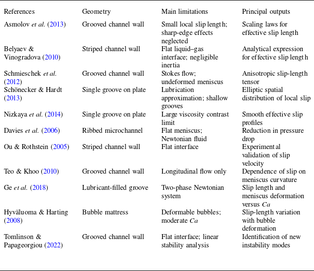
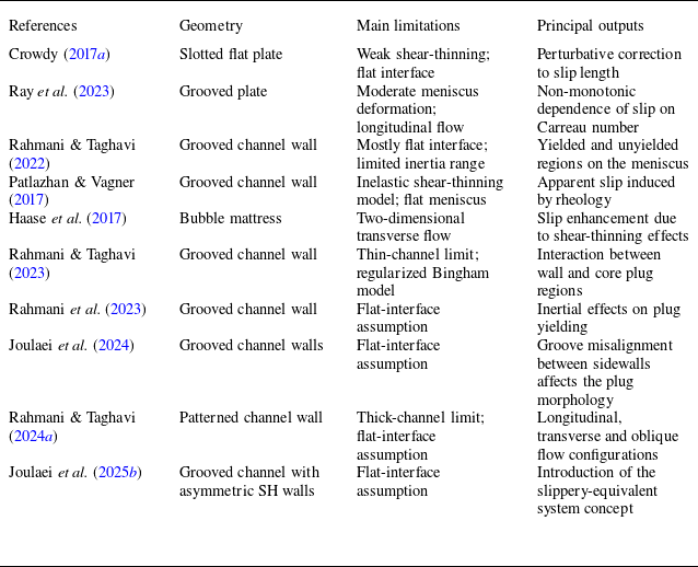
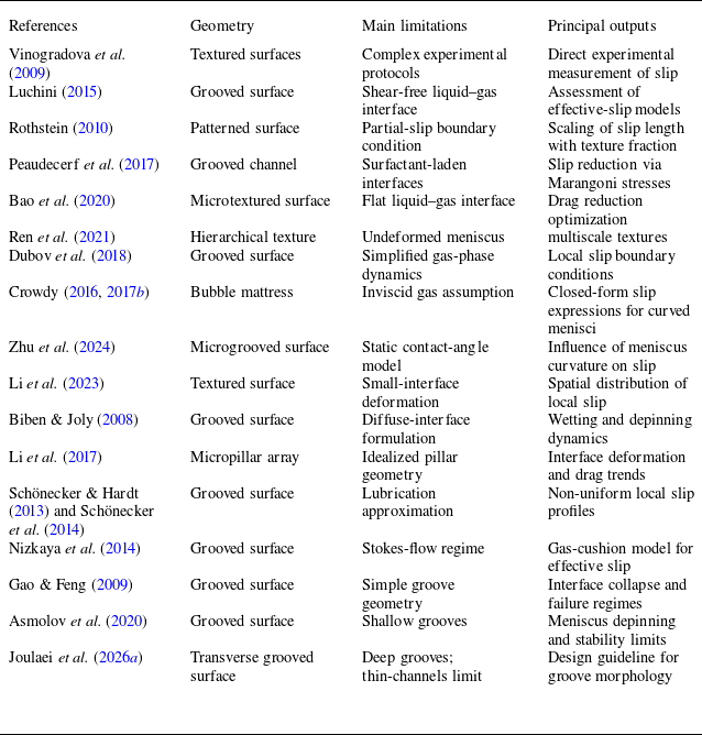

 η^(x^)
 θ
 Θ<135∘
 ⋅^
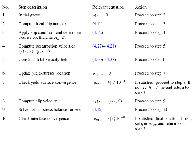
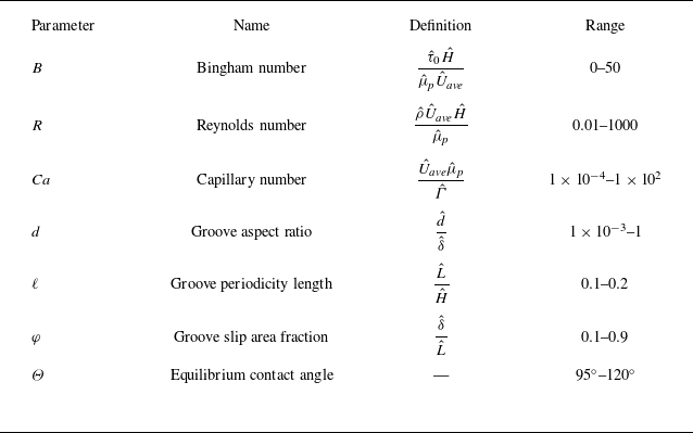
 τ^0
 H^
 μ^p
 U^ave
 δ^
 d^
 L^

 Is
 φ=0.3
 0.5
 0.9
 d=0.05
 B=0.1
 Ca=0.03
 R=0.01
 Θ=95∘
 ℓ=0.2
 h
 hu

 B=0.1
 Ca=0.03
 d=10−2
 Ca=0.03
 B=0.1
 Θ=95∘
 d=10−2
 R=0.01
 ℓ=0.2
 φ=0.5
 η=−1
 Is

 ⟨us⟩
 d
 B=0.1
 1
 10
 Ca=1.37×10⁻⁴
 Ca=1.37×10⁻⁴
 0.01
 0.03
 B=0.1
 ℓ=0.2
 φ=0.5
 Θ=95∘
 R=0.01
 ⟨us⟩
 dcr

 d=0.05
 0.1
 0.2
 0.5
 B=0
 B=10
 R=50
 Ca≈0.69
 ℓ=0.2
 Θ=95∘
 φ=0.5
 B=10

 d
 B=0
 1
 10
 R=50
 R
 d=0.5
 B=10
 Is
 R
 B=10
 d=0.5
 ℓ=0.2
 φ=0.5
 Θ=95∘

 R=0.01
 50
 100
 500
 B=1
 B=10
 d=0.05
 Θ=95∘
 φ=0.5
 ℓ=0.2

 B=0
 1
 10
 Θ=95∘
 Θ=120∘
 d=0.05
 φ=0.5
 ℓ=0.2
 η=−1
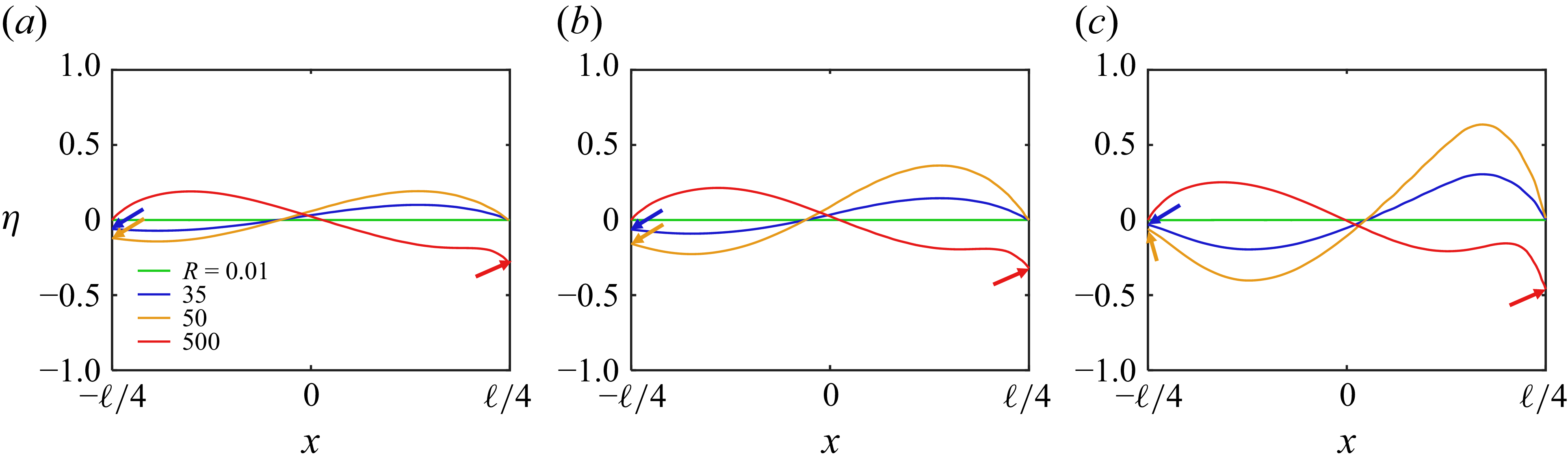
 B=0
 B=1
 B=10
 d=0.05
 φ=0.5
 ℓ=0.2
 Θ=95∘
 θadv=120∘
 θrec=70∘
 η=−1

 d
 R=0.01
 R=50
 R=100
 R=500
 B=10
 φ=0.5
 Θ=95∘
 ℓ=0.2

 ℓ=0.2
 φ=0.5
 d
 B=0.1
 1
 10
 R=0.01
 R=50
 500
 B
 d=0.05
 φ=0.3
 0.5
 0.7
 ℓ=0.2
 ℓ=0.1
 0.2
 φ=0.5
 dcr
 Θ=95∘

 χe,2
 B
 φ
 d
 ℓ=0.2
 ℓ=0.1
 Ca=1.37×10⁻⁴
 R=50
 Θ=95∘

 d
 R
 B=0
 B=1
 B=50
 Θ=95∘
 Θ=120∘
 ×

 (d−R)
 B=0
 B=1
 B=50
 φ=0.5
 ℓ=0.2
 Θ=95∘
 θadv=120∘
 θrec=70∘
 x=−φℓ/2
 x=φℓ/2

 d>0.2
 R∗
 B
 R∗=R/(1+B)
 φ=0.5
 ℓ=0.2
 Θ=95∘
 Θ=120∘
 Θ=95∘
 θadv=120∘
 θrec=70∘
 x=−φℓ/2
 x=φℓ/2
 R∗=30B−1
 R∗=50B−1
 R∗=32B−1
 B>0
 d>0.2

 d
 Ca
 B=0.1
 B=1
 φ=0.5
 ℓ=0.2
 R=0.01
 max(|η|)⩽0.01
 max(|η|)>0.01
 Θ=110∘
 120∘

 B=0.1
 B=1
 Ca=1.37×10⁻⁴
 Θ=95∘

 M
 U
 B=50
 b=0.02
 M
 d=0.5
 R=0.01
 φ=0.5
 ℓ=0.2
 B=10

 (y<0)
 R=0.01
 ℓ=0.2
 φ=0.5
 d=0.05
 B=0.1
 Ca=10−4
 U/u¯s
 u¯s
 y∗=y^/d^

 R=0.13
 Ca=0.5
 φ=0.5
 ℓ=0.25
 Θ=80∘

 B=0
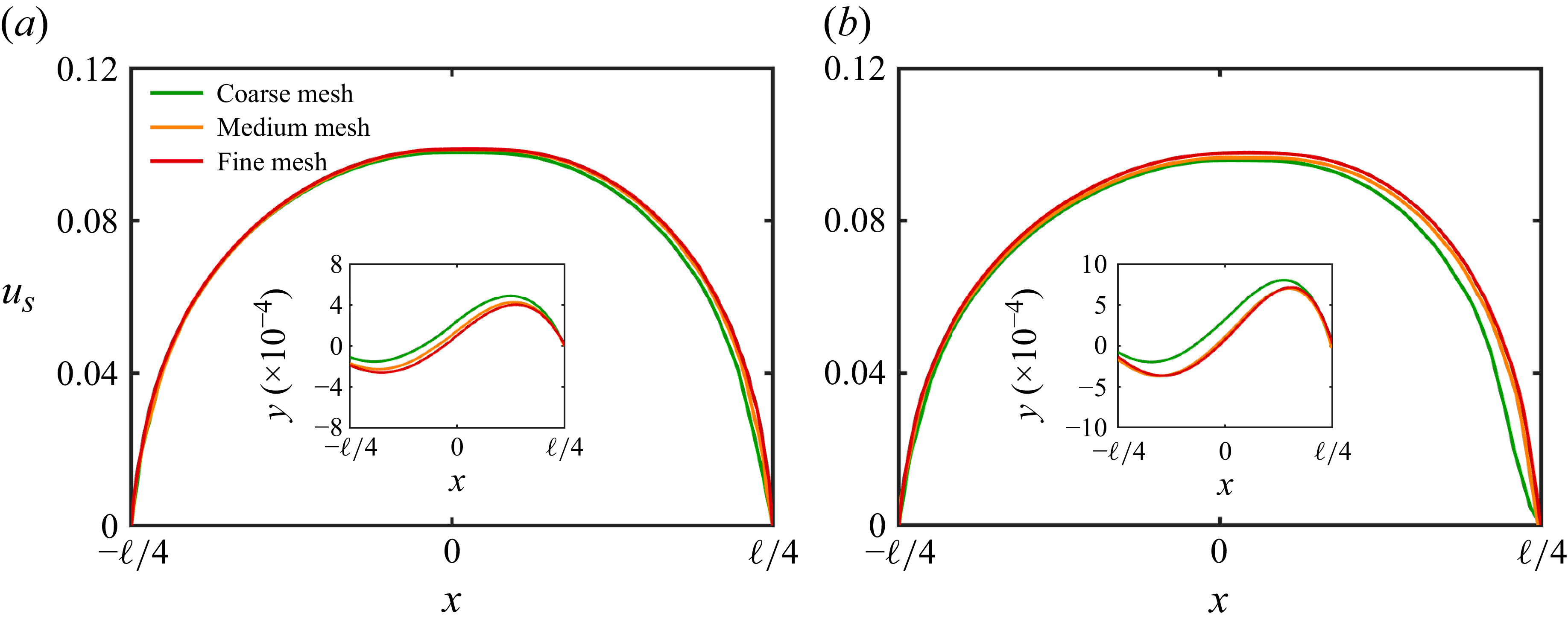
 R=50
 100
 B=1
 d=0.05
 ℓ=0.2
 φ=0.5

 Open access

