

Introduction
Switzerland has numerous indigenous and locally developed sheep breeds. These genetic resources with unique adaptive traits are assumed to respond best to the pressures of the local environment (Glowatzki-Mullis et al., Reference Glowatzki-Mullis, Muntwyler, Bäumle and Gaillard2009). To understand variation within and between local sheep breeds, the regular analysis of available genetic diversity is advised. Pedigree-based analysis of different genetic diversity parameters has been conducted for four main breeds using a generic report for population management named POPREP (Groeneveld et al., Reference Groeneveld, Westhuizen, Maiwashe, Voordewind and Ferraz2009): Swiss White Alpine (SWA), Swiss Black-Brown Mountain sheep (SBS), Valais Blacknose sheep (VBS) and Brown Headed Meat (Burren et al., Reference Burren, Flury, Aeschlimann, Hagger and Rieder2012). For the year 2008, almost 30 000 SWA lambs were produced by SWA, and, for the latter three breeds, about 10 000 lambs were born, according to herdbook records (Burren et al., Reference Burren, Flury, Aeschlimann, Hagger and Rieder2012). Due to the remarkable average inbreeding coefficient of 9.2 percent and an effective population size below 100 regular monitoring of the available genetic diversity was proposed for the VBS breed (Burren et al., Reference Burren, Flury, Aeschlimann, Hagger and Rieder2012), a local breed which is limited to one geographic region of Switzerland.
Beside the four main breeds under scrutiny, Glowatzki-Mullis et al. (Reference Glowatzki-Mullis, Muntwyler, Bäumle and Gaillard2009) investigated the genetic diversity of Engadine Red sheep (ERS), Swiss Mirror sheep (SMS), Valais Red sheep (VRS), East Friesian and Skudden sheep using 44 microsatellites. Using the software program Structure (Pritchard et al., Reference Pritchard, Stephens and Donnelly2000), the two local breeds (VRS and VBS), which originated in the same geographical area, could not be differentiated. In addition, genetic proximity between SWA and SMS was determined. These results were in line with the findings of an earlier study based on 31 microsatellites (Stahlberger-Saitbekova et al., Reference Stahlberger-Saitbekova, Schläpfer, Dolf and Gaillard2001).
Within the International Sheep Genomic Consortium (ISGC), a genome-wide single nucleotide polymorphism (SNP) panel was developed and tested based on genotypes from 2 819 sheep belonging to 74 breeds (Kijas et al., Reference Kijas, Lenstra, Hayes, Boitard, Porto Neto, Cristobal, Servin, McCulloch, Whan, Gietzen, Paiva, Barendse, Ciani, Raadsma, McEwan and Dalrymple2012). Out of these, seven were local sheep breeds from Switzerland. Based on a principal component analysis (PCA), this study showed clear genetic divisions separating European, Asian and African sheep breeds. Even though: aspects of genetic diversity and fine-scale populations of local Swiss breeds are only sparsely covered by these authors. Therefore, the public available genotypes from 168 individuals of seven Swiss breeds (SWA, SBS, VBS, ERS, SMS, VRS and Bundner Oberländer sheep (BOS)) were isolated from the ISGC (Kijas et al., Reference Kijas, Lenstra, Hayes, Boitard, Porto Neto, Cristobal, Servin, McCulloch, Whan, Gietzen, Paiva, Barendse, Ciani, Raadsma, McEwan and Dalrymple2012) and re-analysed with special focus on genetic diversity of local Swiss breeds. The primary goal of the current study was to investigate fine-scale population structures within and between Swiss sheep breeds using dense SNP data and applying network-based clustering methods. The results are compared with results from earlier studies based on microsatellites. Potential needs for genetic monitoring and conservation activities are underlined.
Material and methods
Data
The sheep breeds used in this study were previously described in detail by Kijas et al. (Reference Kijas, Lenstra, Hayes, Boitard, Porto Neto, Cristobal, Servin, McCulloch, Whan, Gietzen, Paiva, Barendse, Ciani, Raadsma, McEwan and Dalrymple2012). During the trial, 24 individuals from each of the seven indigenous Swiss sheep breeds were genotyped using the Illumina Ovine SNP50 BeadChip (Kijas et al., Reference Kijas, Lenstra, Hayes, Boitard, Porto Neto, Cristobal, Servin, McCulloch, Whan, Gietzen, Paiva, Barendse, Ciani, Raadsma, McEwan and Dalrymple2012). In the sheep HapMap project, it was subjected that a breed includes at least one parent–offspring pair, therefore some of the individuals included in the data sample are known relatives to each other (Kijas et al., Reference Kijas, Lenstra, Hayes, Boitard, Porto Neto, Cristobal, Servin, McCulloch, Whan, Gietzen, Paiva, Barendse, Ciani, Raadsma, McEwan and Dalrymple2012) and these relationship were described in the data release. Totally, the analysed data set comprised 20 trios (i.e. genotyped individual and genotypes for both parents) (Table S1). Beside this information, no more pedigree information was available for genotyped individuals.
The data set was filtered using Plink-1.07 (Purcell et al., Reference Purcell, Neale, Todd-Brown, Thomas, Ferreira, Bender, Maller, Sklar, de Bakker, Daly and Sham2007). Firstly, non-annotated SNPs or SNPs with missing positions were removed. Secondly, SNPs with a minor allele frequency below 0.05, with more than 10 percent missing genotypes per marker or per individual, or those deviating from Hardy–Weinberg equilibrium (p = 0.0001) were excluded. 45 193 SNPs (92 percent) from the initial available 49 034 SNPs passed the filtering procedure. Using quality filtered SNPs, the genome-wide proportions of shared alleles identical by descent (IBD) between all samples were calculated using Plink-1.07. The estimated genomic relationship (pi-hat) between two samples from the VRS breed was 100 percent (identical) and so one duplicate genotype was excluded from further analysis. Due to restricted sample size, the genotypic information for 20 trios was not omitted from the final analysis. Finally, the genotypic information from a total of 167 individuals and 45 193 SNPs covering 26 ovine autosomes was considered for the population structure analysis.
Cluster analysis and genomic relationships
The program Admixture (Alexander, Novembre and Lange, Reference Alexander, Novembre and Lange2009) was used to determine the optimal number of k clusters and for assigning individuals to their true clusters. The algorithms implemented in Admixture are considered to be computationally more efficient (Alexander, Novembre and Lange, Reference Alexander, Novembre and Lange2009) than the algorithms implemented in the software Structure (Pritchard et al., Reference Pritchard, Stephens and Donnelly2000) and can be easily applied on genome-wide data sets to infer individual ancestry. By adding the –cv flag, Admixture includes a cross-validation procedure that allows identification of the optimal value of k for which the model has best predictive accuracy (Alexander, Novembre and Lange, Reference Alexander, Novembre and Lange2009). Within this analysis, –cv was set to 10, and the k with the lowest cross-validation error was used for the choice of the optimal number of clusters for the set of genotypes under investigation. The software Distruct (Rosenberg, Reference Rosenberg2004) was used for the graphical presentation of each cluster assignment increasing k from 2 to 8.
Due to the availability of large numbers of SNPs, it was possible to calculate genome-wide IBD or identical by state (IBS) between samples using the Plink-1.07 (Purcell et al., Reference Purcell, Neale, Todd-Brown, Thomas, Ferreira, Bender, Maller, Sklar, de Bakker, Daly and Sham2007) option –genome. This option was used to estimate the genome-wide proportions of IBD (pi-hat) between individuals. The estimated proportions of IBD were graphically converted using the R-function levelplot of the package lattice (Sarkar, Reference Sarkar2008).
Besides the model-based cluster analysis, we further investigated the population structure of sheep breeds using PCA and multi-dimensional scaling (MDS). PCA and MDS are non-parametric approaches, which utilize pairwise relationships between individuals for the final visualization of genome-wide population structures.
PCA identified the principal components that represented the population structure based on genetic correlations (shared ibs segments) between individuals, whereas MDS identified dimensions that explained observed genetic distance between individuals (Wang et al., Reference Wang, Sun, Stand, Berlin, Wilcos and Li2009). For MDS analysis, genome-wide pairwise ibs-distances between individuals were used in conjunction with the –mds-plot –cluster = 3 option in Plink-1.07 (Purcell et al., Reference Purcell, Neale, Todd-Brown, Thomas, Ferreira, Bender, Maller, Sklar, de Bakker, Daly and Sham2007). The MDS plot was created using the R-package scatterplot3d (Ligges and Mächler, Reference Ligges and Mächler2003).
Finally, we used high definition network visualization for the available SNP genotypes to detect fine-scale population structures within and between sheep breeds (Neuditschko, Kathkar and Raadsma, Reference Neuditschko, Kathkar and Raadsma2012). The so-called NetView approach (Neuditschko, Kathkar and Raadsma, Reference Neuditschko, Kathkar and Raadsma2012) consists of five distinct components: data preparation and editing, calculation of a genetic-relationship or genetic distance matrix among all individuals and samples, network construction, clustering of individuals within the population network and finally, the visualization of the clustering results using the software Cytoscape (Shannon et al., Reference Shannon, Markiel, Ozier, Baliga, Wang, Ramage, Amin, Schwikowski and Ideker2003). The number of nearest neighbours (k-NN) was set equal 10. For additional visualization of hierarchical population structures, the R-package phytools (Revell, Reference Revell2012) was applied. Thickness of lines connecting individuals was set in proportion to ibs-distances between individuals (i.e. ibs-distances >0.8 = thick line; ibs-distances <0.8 = thin line).
Phylogenetic analysis
To evaluate the general hierarchical population structure of the sheep breeds, pairwise FST-values were calculated among the seven sheep breeds from population allele frequencies across all 45 193 autosomal SNPs using the program package Genepop 4.1.4 (Rousset, Reference Rousset2008). For the graphical presentation of phylogenetic relationships between the seven breeds, the common applied neighbour-joining (NJ)-method was chosen, as implemented in the program Splitstree4 (Huson and Bryant, Reference Huson and Bryant2006).
Derivation of linkage disequilibrium (LD) and estimation of effective population size (N e)
Plink-1.07 (Purcell et al., Reference Purcell, Neale, Todd-Brown, Thomas, Ferreira, Bender, Maller, Sklar, de Bakker, Daly and Sham2007) was used to estimate pairwise LD between SNPs. r 2-values over all 26 autosomes were grouped according to their physical intermarker-distances, assuming a constant recombination rate, and were then averaged for distance bins of 50 kb. The smallest bin ranged from 0 to 50 kb and the largest from 1 950 to 2 000 kb, resulting in bins with a minimum average intermarker-distance of 25 kb up to a maximum of 1 975 kb. To derive estimates of recent effective population sizes (i.e. N e five or ten generations ago) two ‘maxi’-bins for pairs of SNPs with an average intermarker-distance of 4 975 and 9 975 kb, respectively, were created.
For the derivation of N e, Sved's equation (Sved, Reference Sved1971) was applied
 $$E\lpar {r^2}\rpar =1/\lpar 1+4{N_{\rm e}}c\rpar .$$
In the case of restricted sample sizes, Weir and Hill (Reference Weir and Hill1980) proposed that the equation be completed using the term (1/n). Thus, the equation was converted allowing for an estimation of N e
 $$E\lpar {r^2}\rpar =1/\lpar 1+4{N_{\rm e}}c\rpar +1{\rm /}n\comma \;$$
where E(r 2 ) is the expectation of the correlation between allele frequencies of two loci, n is 2* sampled animals, c is the genetic distance between loci in Morgan and N e is the effective population size. The genetic distance between SNPs (c) was approximated by setting 1 Mb equal to 0.01 Morgan. Applying this formula, N e was estimated for 1/2c previous generations (Hayes et al., Reference Hayes, Visscher, McPartlan and Goddard2003).
Results
Cluster analysis and genomic relationships
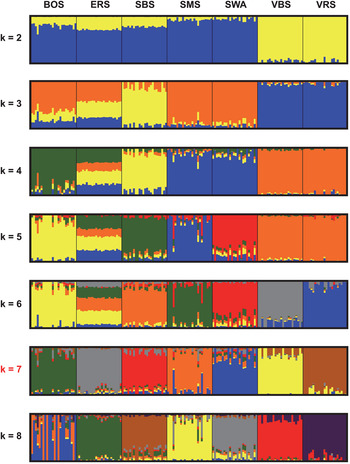
The graphical visualization of the results from cluster analysis of the 167 animals for k ranging from two to eight clusters is shown in Figure 1. The cross-validation error was assessed to define the optimal value for k for the different number of clusters (Supplementary Figure S2). The cross-validation error decreased to k = 7 and then increased again. Therefore, k = 7 was determined to be an optimal number of clusters for the analysis given in Figure 1.
Results cluster analysis for k = 2–8. Based on the cross-validation k = 7 had the best fit and is therefore indicated in red.

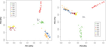
The first principal component (PC1) explained 25 percent of the observed variation (Figure 2), the second (PC2) 8 percent and the third (PC3) 7 percent, respectively. The separation of the seven breeds was obvious by contrasting PC1 versus PC2 and PC2 versus PC3. The first component identified the separation of the Valais breeds (VBS and VRS) from the other breeds, whereas the second component showed the separation between SBS, ERS and BOS, as well as SMS and SWA. Using the third component, the separation between BOS and ERS became clearer, whereas the Valais breeds (VBS and VRS) and SMS had higher connection with SWA. The MDS plot is given in Supplementary Figure S1.
PCA for the seven breeds

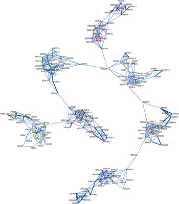
The visualization of the investigated network for the data is given in Figure 3. The thickness of the lines varies in proportion with the genetic distance and is used to visualize the individual relationships within and between populations. The node size varied in proportion to the numbers of edges per node, and illustrated how well each individual was connected within the population (Neuditschko, Kathkar and Raadsma, 2012).
Organic NetView for the seven breeds (yellow: VBS, brown: VRS, green: BOS, red: SBS, grey: ERS, orange SMS and blue: SWA).

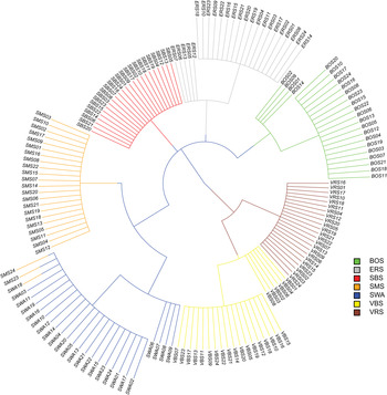
Additionally, the network-based-cluster tree is given in Figure 4, where each breed is represented by the same colour as in Figure 3. At the base of the tree, the Valais breeds (VBS and VRS) were separated from the other five breeds. At the second level, all breeds were assigned into distinct clusters, except SMS and SWA individuals. At the third level substructures within BOS, ERS and the VBS breed became visible, while VRS, SBS and SMS reflect homogenous samples. Additionally, SWA and SMS were clustered according to the initial breed assignment into distinct groups, except two SMS individuals (SMS24 and SMS23). Substructure in SWA occurred at the fourth and the final level of the tree.
Network-based-cluster tree for the seven breeds (thick lines equal ibs-distances >0.8 and thin lines equal ibs-distances <0.8).

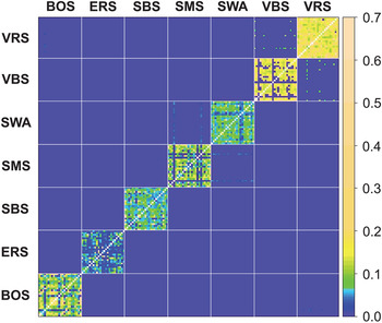
Genomic relationships within and between breeds are given in Figure 5. The average genomic relationships (within breeds) varied from 5 percent (ERS), 9 percent (SBS), 9 percent (SWA), 10 percent (SMS), 12 percent (BOS), 12 percent (VBS) to 20 percent (VRS). Some genomic relationships (>0 between populations) were found for two SMS individuals (SMS24 and SMS23) and SWA (light blue), for some VRS individuals with VBS (light green) and for one BOS individual with VRS. Estimated genomic relationships between the 20 offspring with their genotyped parents are given in Supplementary Table S1. For seven offspring genomic relationships below 0.35 with one parent were found.
Genomic relationships within and between breeds (the colour scale for the levels of genomic relationships is given at the right end of the matrix).

Phylogenetic analysis
The NJ-tree (Supplementary Figure S3) represents the phylogenetic relationships for the seven Swiss sheep breeds based on FST-distances. VBS and VRS were found to be clearly distinct from other breeds. SWA and SMS were also on a separate branch, but less far away from the other breeds. The shortest FST-distance was found between SBS and ERS breeds.
Marker-based estimation of effective population size
Estimates of pairwise LD between SNPs for different distance bins were used to derive effective population sizes for the seven Swiss sheep breeds investigated. The result for the development of N e over the last 2 000 generations for all breeds is shown in Supplementary Figure S4, where the population sizes for all seven breeds showed a decreasing trend. Based on the two maxi bins, estimates for recent N e (last five to ten generations) as 18–35 for SBS, 27–44 for VRS, 26–47 for BOS, 29–49 for SMS, 29–58 for VBS, 30–58 for ERS and 31–66 for SWA, respectively, were determined.
Discussion
Genetic diversity between breeds
Based on the PCA results (Figure 2) and the MDS plot (Supplementary Figure S1), the seven breeds can be clustered into five distinct groups with evidence of additional sub-structures. The three breeds, BOS, SBS and ERS, comprised distinct groups, whereby VBS/VRS and SMS/SWA individuals were not clearly separated from each other. The proximity between VBS/VRS and SMS/SWA was further supported by the Admixture and NetView analysis presented in Figures 1 and 4, while these two methods divide the individuals into seven respective breed groups. However, based on these results, it was assumed that the proximities within these two clusters are of different origin. VBS and VRS are local Swiss alpine breeds, which are geographically restricted to the canton of Valais. The differentiation of these two breeds from the other five breeds was supported by data shown in Figure 1, i.e. from k = 2 to 5, the two breeds clustered together and are clearly distinct from all others. In Figure 4, VBS and VRS are separated from the other breeds at the base of the tree. Data illustrated in Figure S3 showed that the common branch connecting the two breeds with the other breeds is quite long. Therefore, it was assumed that the geographical differences for these two breeds compared with the other breeds is, genetically, rather old. The proximity between VRS and VBS was determined using 44 microsatellites (Glowatzki-Mullis et al., Reference Glowatzki-Mullis, Muntwyler, Bäumle and Gaillard2009) and 31 microsatellites (Stahlberger-Saitbekova et al., Reference Stahlberger-Saitbekova, Schläpfer, Dolf and Gaillard2001). Based on PCA, Kijas et al. (Reference Kijas, Lenstra, Hayes, Boitard, Porto Neto, Cristobal, Servin, McCulloch, Whan, Gietzen, Paiva, Barendse, Ciani, Raadsma, McEwan and Dalrymple2012) found the two Valais breeds to be genetically distinct from the other breeds. Based on their genetic uniqueness, a high potential for conservation is attributed to these two breeds.
Network visualization (Figure 3) showed that VRS21 was related to BOS07. This relationship was supported by four genomic relationships that were slightly greater than zero (0.0376, 0.0283, 0.0251 and 0.0247) between this VRS individual and two BOS individuals (Figure 5). This connection was thought to originate from breeding practices over the last 20 years. Four sheep breeds (BOS, ERS, SMS and VRS) were not officially annotated before 1999. In the year 1982, the foundation ‘ProSpecieRara’ was created to promote plant and livestock genetic resources (FOAG, 2007). The foundation collected remaining animals of these four sheep breeds and supported farms keeping such individuals. Therefore, it is possible that a certain exchange between these breeds happened by chance on farms with small herds of different breeds or before the collection of remaining individuals.
The similarity between SMS and SWA was supported by Glowatzki-Mullis et al. (Reference Glowatzki-Mullis, Muntwyler, Bäumle and Gaillard2009), Stahlberger-Saitbekova et al. (Reference Stahlberger-Saitbekova, Schläpfer, Dolf and Gaillard2001) and Kijas et al. (Reference Kijas, Lenstra, Hayes, Boitard, Porto Neto, Cristobal, Servin, McCulloch, Whan, Gietzen, Paiva, Barendse, Ciani, Raadsma, McEwan and Dalrymple2012). The SMS is a descendant of the ancient Grisons breed (FOAG, 2007) and, as stated previously, was not officially annotated until 1999. The main visual differentiation between SMS and SWA are the dark-haired patterns found in SMS animals around the mouth and the eyes (resembling spectacles). It is expected that crossbreeding with SWA – the most popular sheep breed in Switzerland – occurred in the recent past before the breeding programme for SMS started (Stahlberger-Saitbekova et al., Reference Stahlberger-Saitbekova, Schläpfer, Dolf and Gaillard2001; Glowatzki-Mullis et al., Reference Glowatzki-Mullis, Muntwyler, Bäumle and Gaillard2009). The results from network-analysis (Figure 3) showed that one SMS individual (SMS23) fell between the SMS and the SWA clusters and one individual from SMS (SMS24) lay in the SWA cluster, which is related to SMS. The first individual was assumed to be a crossbred with SWA, although for the second sheep, a wrong breed assignment of the sampled DNA could be an explanation. In Figure 4, these two individuals were grouped into the SWA cluster. In Figure 5, these two SMS individuals could be recognized, based on the genomic relationships. They were almost certainly not related to the majority of the other individuals from the SMS sample, but showed a certain relationship with many individuals of the SWA breed. Unfortunately, animal identities were not available and therefore the retrospective reconstruction of such connections based on herdbook-information was not possible.
The results for the ERS breed were also interesting. In the PCA plot (Figure 2) and the MDS plot (Supplementary Figure S1), the sample group for the ERS fell between all the other clusters. Based on the results from Admixture (Alexander, Novembre and Lange, Reference Alexander, Novembre and Lange2009) for k = 3–6, the breed seemed to be a conglomerate of genetic resources from different origins (Figure 1). However, with k = 7, ERS became clearly distinguishable from the other clusters. The specific pattern of the ERS sample was not observed in a cluster analysis based on 41 microsatellites (Glowatzki-Mullis et al., Reference Glowatzki-Mullis, Muntwyler, Bäumle and Gaillard2009). The network visualization allowed a more detailed understanding of connections between individuals of the ERS sample to individuals of the other breeds (Figure 3). One ERS individual fell outside the ERS cluster and had connections to individuals from the BOS and SBS breeds. Additionally, this individual was directly related to an ERS individual that was connected to an outlier of the SMS breed (Figure 3). According to the data shown in Supplementary Figure S3, the differentiation time was shortest between ERS and SBS, followed by BOS. However, no genomic relationships (>0) could be found between the 24 ERS individuals and those from the SBS and BOS samples. The origins of the ERS can be traced back to the Stone sheep of the Eastern Alps and the Bergamasca sheep (FOAG, 2007). In a recently published study, the genetic relationships between Italian sheep breeds and other European sheep breeds were derived using genome-wide SNP data (Ciani et al., Reference Ciani, Crepaldi, Nicoloso, Lasagna, Sarti, Moioli, Napolitano, Carta, Usai, D'Andrea, Marletta, Ciampolini, Riggio, Occidente, Matassino, Kompan, Modesto, Macciotta, Ajmone-Marsan and Pilla2014). This study confirms the known proximity between ERS and the Bergamasca breed at molecular level as ERS clustered closest to this Italian breed in a NJ tree based on Reynolds-genetic distances. Hence, for the ERS breed it is concluded, that the consideration of samples from Swiss sheep breeds only, limits the understanding of its fine-scale population structures.
Genetic diversity within breeds
Average genomic relationships within breeds ranged from 5 percent (ERS) to 20 percent (VRS) (Figure 5). As previously stated, the VRS breed is historically restricted to a single region in the canton Valais. Furthermore, the actual population size of VRS is considerably small (about 1 000 herdbook individuals). With average genomic relationships of 12 percent, the VBS and BOS breeds showed the second highest average genomic relationships within breed. Based on pedigree information, an average inbreeding coefficient of 9.2 percent was found for the 10 000 VBS individuals born in the year 2008 (Burren et al., Reference Burren, Flury, Aeschlimann, Hagger and Rieder2012). For SBS, SMS and SWA breeds, the average genomic relationships ranged from 9 to 10 percent. The lowest average genomic relationships within the ERS sample was not surprising due to the known historic influences of different breeds mentioned above. The availability of dense SNP data allows the derivation of pairwise genomic relationships when pedigree information is missing (Hasler et al., Reference Hasler, Flury, Menet, Haase, Leeb, Simianer, Poncet and Rieder2011). The genomic relationships of parent–offspring pairs for the 20 trio indicated in the initial file are given in Supplementary Table S1. For seven offspring, the estimated genomic relationships with one parent were found to be lower than 0.35. Due to the remarkable discrepancy of the realized genomic relationships from the expected relationships (eq. (0.5)) it assumed that the indication of six sires and one dam for these seven offspring is not correct. This finding was further supported by missing thick lines between these pairs in Figure 4.
NetView visualization demonstrated that the samples for all breeds showed a certain substructure (Figures 3 and 4). Reasons for this could include the sampling procedure (i.e. sampling related individuals from one herd) and crossbreeding. The substructure of the VBS and the SWA sample (Figures 3 and 4) is mainly a fact of the sampling of directly related animals (i.e. trio). The two main Swiss sheep breeds SWA and SBS are especially known to be influenced by other European sheep breeds. This result was supported by Kijas et al. (Reference Kijas, Lenstra, Hayes, Boitard, Porto Neto, Cristobal, Servin, McCulloch, Whan, Gietzen, Paiva, Barendse, Ciani, Raadsma, McEwan and Dalrymple2012), where SWA, SBS and SMS were in an intermediate position in the PCA of European sheep breeds.
Estimates of ancestral and recent N e for the seven sheep breeds based on SNP data are shown in Supplementary Figure S4. The N e showed a decreasing trend over the last 2 000 generations, with an increasingly steeper slope since about 700 generations ago. The highest historically effective population size was found for ERS and the lowest for SMS. For recent effective population sizes, the estimates varied from 18 (SBS) to 31 (SWA) five generations ago, to 35 (SBS) and 66 (SWA) ten generations ago. Generally, the differences for recent effective population sizes between breeds were rather small. However, as some of the investigated samples were influenced by admixture and restricted sample sizes, those estimates should be interpreted with caution (Corbin et al., Reference Corbin, Liu, Bishop and Woolliams2012).
Based on the genetic uniqueness of the VRS and the VBS breed and the high level of relatedness within those two breeds, the implementation of monitoring programmes to control genetic diversity in daily breeding practice is proposed. For the other breeds, regular monitoring of genetic diversity is advised.
Conclusions
Genomic relationships greater than zero were found for some individuals from different breeds. Thus having genome-wide SNP data available, it is possible to overcome the limitation of pedigree information and derive genomic relationships between breeds. The results related to general population structures are comparable with those from earlier studies based on microsatellites. However, dense SNP data used here in combination with network-theory allowed for a more detailed analysis of fine-scale population structures of seven Swiss sheep breeds. The two geographically separated breeds, VBS and VRS, are clearly distinct from the other Swiss sheep breeds and show remarkable genomic relationships within population. Therefore, the implementation of mechanisms to control genetic diversity is proposed for these breeds.
Acknowledgements
The Swiss Federal Office of Agriculture is acknowledged for the financial support of the costs for genotyping. Lucy Waldron is acknowledged for grateful support related to language editing.