3.1. Statistically averaged quantities

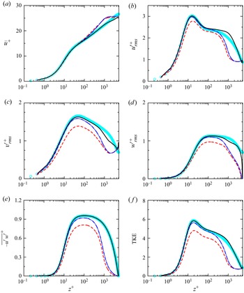
Figure 1 shows the mean streamwise velocity profiles ($\bar {u}^+$) and profiles of root-mean-square (r.m.s.) of velocity fluctuations ($u'^+_{rms}$, $v'^{+}_{rms}$ and $w'^{+}_{rms}$), turbulent Reynolds stress ($-\overline {u'w'}^{+}$) and TKE of the carrier phase. For the unladen case, the present DNS results are compared with the DNS results of turbulent channel flow at $Re_{\tau } = 5186$ from Lee & Moser (Reference Lee and Moser2015). For $z^+ \le 1000$, the mean streamwise velocity profile in the open channel compares well with the closed channel, and a distinct wake region can be observed in both unladen and laden cases for $z^+ > 1000$. Here $u'^+_{rms}$ compares well in the inner layer (i.e. $z^+ \le 100$), whereas $v'^{+}_{rms}$ and $w'^{+}_{rms}$ compare well in a slightly larger region (i.e. $z^+ \le 500$). We find that $-\overline {u'w'}^{+}$ compares well across the channel height, but the TKE shows similar behaviour as the r.m.s. of velocity fluctuations. The peak values of r.m.s. velocity fluctuations and the corresponding locations matches well with the closed channel. Differences in the outer layer are attributed to the differences in channel versus open channel flow near the centreline/boundary, i.e. blocking effect of the shear-free condition on the free surface (Calmet & Magnaudet Reference Calmet and Magnaudet2003).

Figure 1.

(a) Mean streamwise velocity profile and (b–f) profiles of r.m.s. of velocity fluctuations: (b) $u'^+_{rms}$, (c) $v'^{+}_{rms}$, (d) $w'^{+}_{rms}$, (e) $\overline {u'w'}^{+}$ and ( f) TKE; ($\circ$, cyan), DNS results from Lee & Moser (Reference Lee and Moser2015); ——, present DNS results for the unladen case (C0); – – – –, high-$St$ case (C1); —$\cdot$—, low-$St$ case (C2). Values in all panels are normalised by viscous scales.

For the particle-laden cases, the mean streamwise velocity profiles tend to follow the log-law with a smaller Kármán constant for $30 \le z^+ \le 1000$, and a distinct wake region can also be observed for $z^+ > 1000$, which is noticeably flatter than the unladen case. The r.m.s. velocity fluctuations, turbulent Reynolds stress and TKE are all reduced compared with the unladen case, and this suppression is strongest for the high-$St$ particles. These modifications to first- and second-order statistics are generally consistent with the observations in both experimental (Righetti & Romano Reference Righetti and Romano2004) and numerical investigations (Dritselis & Vlachos Reference Dritselis and Vlachos2008; Zhao, Andersson & Gillissen Reference Zhao, Andersson and Gillissen2010; Lee & Lee Reference Lee and Lee2015; Vreman Reference Vreman2015), with some exceptions (particularly in the changes to $u'^+_{rms}$). Meanwhile, the peak locations are the same as for the unladen case.

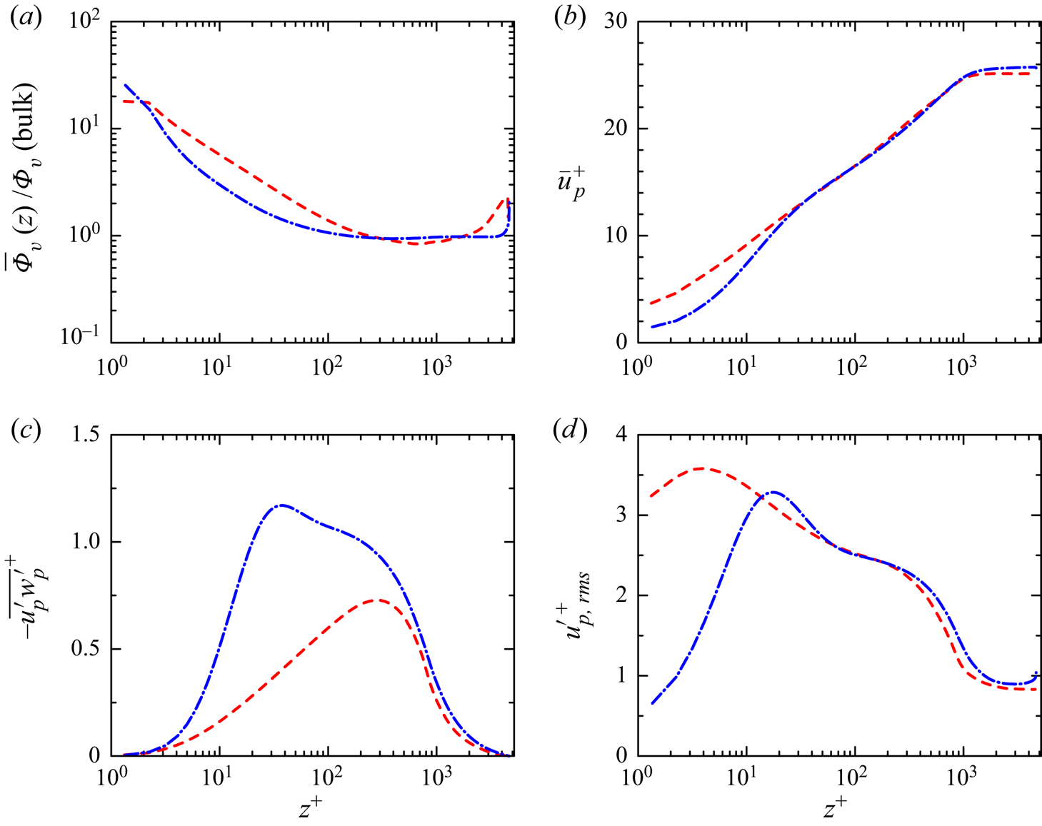
Figure 2 shows the distributions of the mean particle volume concentration ($\bar {\varPhi }_v$), mean streamwise particle velocity ($\bar {u}_p^+$), particle Reynolds stresses ($-\overline {u'_p w'_p}^+$) and r.m.s. particle streamwise velocity fluctuations ($u'^+_{p,rms}$). In addition to the near-wall preferential accumulation, the particles also exhibit a tendency to accumulate preferentially near the free surface, which is observed by Jie, Andersson & Zhao (Reference Jie, Andersson and Zhao2021) in particle-laden channel flow at $Re_{\tau } =600$ but missing in low-$Re_{\tau }$ flows, due to the existence of a quiescent core region characterised by relatively uniform velocity magnitude and weak turbulence levels. This is ultimately a result of turbophoresis due to the gradient of TKE. The near-surface particle accumulation is also observed by Fornari et al. (Reference Fornari, Formenti, Picano and Brandt2016) and Yu et al. (Reference Yu, Lin, Shao and Wang2017) in channel flow laden with finite-size particles ($Re_{\tau } = 180$), but they attributed the particle migration towards the channel centre to particle collision and turbulence–particle interactions, respectively. For $z^+ < 30$, the streamwise particle velocity profile for the low-$St$ case transitions from a logarithmic to a linear behaviour, whereas for the high-$St$ case no linear law is observed; this is also reported by Righetti & Romano (Reference Righetti and Romano2004). The particle Reynolds stress is important for particle deposition in wall-bounded turbulent flows (Young & Leeming Reference Young and Leeming1997). It is found that $-\overline {u'_p w'_p}^+$ increases with decreasing $\bar {\varPhi }_v$ (see also Zhu, Yu & Shao Reference Zhu, Yu and Shao2018), and then decreases to zero at the free surface; however, the peak location of $-\overline {u'_p w'_p}^+$ is smaller than the location of lowest $\bar {\varPhi }_v$. The low-$St$ case exhibits larger $-\overline {u'_p w'_p}^+$, which is similar to r.m.s. velocity fluctuations of the carrier phase (see figure 1). R.m.s. particle streamwise velocity fluctuations $u'^+_{p,rms}$ for the low-$St$ case display a similar behaviour as the carrier phase, but the peak location of the high-$St$ case is closer to the wall, due to their more ballistic trajectories and collisions with the wall, which produce larger differences between the fluid and particle phases (i.e. slip velocity).

Figure 2.

(a) Distributions of the mean particle volume concentration $\bar {\varPhi }_v$ along the wall-normal direction, scaled by the bulk mean concentration $\varPhi _v$. (b) Mean streamwise particle velocity, $\bar {u}_p^+$. (c) Particle Reynolds stress, $-\overline {u'_p w'_p}^+$. (d) R.m.s. of particle streamwise velocity fluctuations, $u'^+_{p,rms}$. Curves:– – – –, high-$St$ case (C1); —$\cdot$—, low-$St$ case (C2). Values in (b,c,d) are normalised by $u_{\tau }$.

3.2. Momentum exchange and interphasial energy transfer

The slip velocity describes the exchange of momentum between the fluid and particle phases. An accurate characterisation of the slip velocities is essential to the modelling of particle trajectories in particle-laden LES (Fede & Simonin Reference Fede and Simonin2006), Reynolds-averaged Navier–Stokes (RANS)-based particle dispersion models (Arcen & Tanière Reference Arcen and Tanière2009), two-fluid model development (Simonin, Deutsch & Minier Reference Simonin, Deutsch and Minier1993), etc. The reaction force, directly related with the slip velocity, governs the particle trajectories and segregation (Marchioli & Soldati Reference Marchioli and Soldati2002), and subsequently modulates the turbulent flow (Tanaka & Eaton Reference Tanaka and Eaton2008; Zhao, Andersson & Gillissen Reference Zhao, Andersson and Gillissen2013).

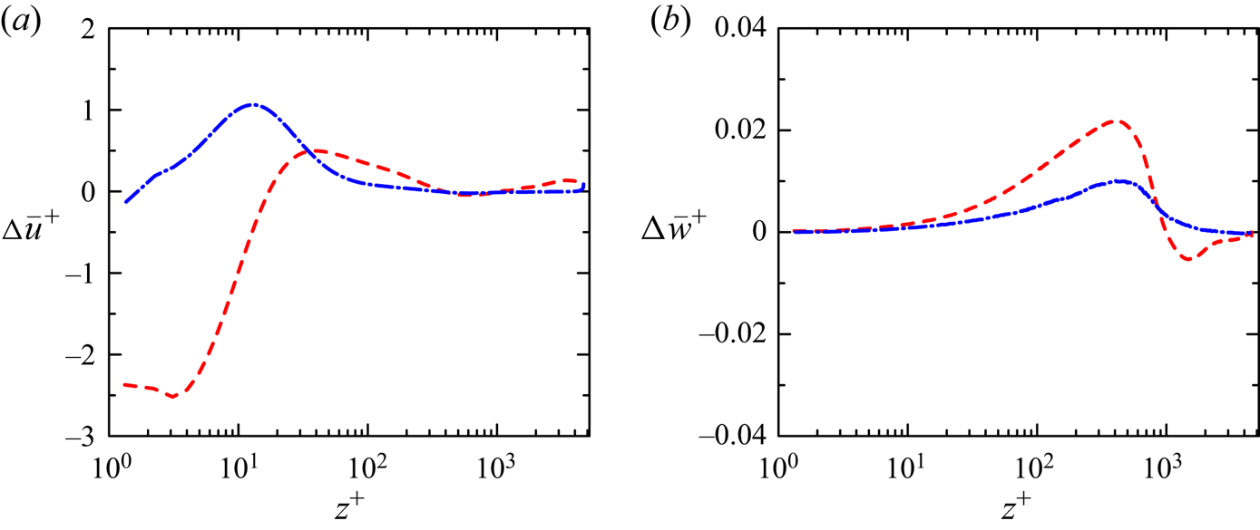
The streamwise and wall-normal slip velocity, i.e. $\Delta \bar {u}^+$ and $\Delta \bar {w}^+$, are shown in figure 3. In the streamwise direction, Zhao, Marchioli & Andersson (Reference Zhao, Marchioli and Andersson2012) found that particles tend to lead the fluid ($\Delta \bar {u}^+<0$) for $z^+< 20$, whereas lag behind the fluid ($\Delta \bar {u}^+>0$) for $z^+> 20$. This behaviour is confirmed in our high-$St$ case, however, the low-inertia particles always lag behind the fluid, except very close to the wall ($z^+<1.5$). In the wall-normal direction, Zhao et al. (Reference Zhao, Marchioli and Andersson2012) found that particles tend to lead the fluid ($\Delta \bar {w}^+<0$) for $z^+<50$, whereas lag behind the fluid ($\Delta \bar {w}^+>0$) for $z^+> 50$. Two distinct regions can also be observed in the high-$St$ case, and the transition is located at approximately $z^+=1000$. The low-inertia particles (C2) always tend to lag behind the fluid, similar to $\Delta \bar {u}^+$. The magnitude of the slip velocity increases with particle inertia, which indicates that the adaption of particles to the fluid motion is reduced with increasing inertia (Zhao et al. Reference Zhao, Marchioli and Andersson2012). Muste & Patel (Reference Muste and Patel1997) experimentally found that $\Delta \bar {u}^+$ increases with the particle concentration (while referring to constant particle diameter). In the present DNS, the streamwise slip velocity seems to be associated with $\bar {\varPhi }_v$, i.e. for $z^+>200$, $\Delta \bar {u}^+$ tends to be zero when $\bar {\varPhi }_v$ approaches the bulk mean volume concentration.

Figure 3.

(a) Streamwise slip velocity $\Delta \bar {u}^+ = (\bar {u}-\bar {u}_p)/{u_{\tau }}$ and (b) wall-normal slip velocity $\Delta \bar {w}^+ = (\bar {w}-\bar {w}_p)/{u_{\tau }}$. Curves: – – – –, high-$St$ case (C1); —$\cdot$—, low-$St$ case (C2).

To gain further insight, we examine the streamwise momentum balance. The total stress $\tau (z)$ can be given by the integral of the streamwise mean momentum equation from $h$ to $z$,

(3.1)\begin{equation} \tau (z) = \rho \nu \frac{\partial \bar{u}}{\partial z} - \rho \overline{u'w'} + \rho \int_h^z \bar{F}_x(z')\,{\rm d} z' = \rho u^2_{\tau} \left(1-\frac{z}{h} \right), \end{equation}

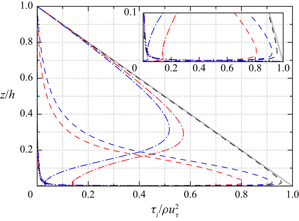
where $\bar {F}_x$ is the mean horizontal feedback force. The first and second terms on the right-hand side of (3.1) denote the fluid viscous and turbulent Reynolds stresses, and the third term is the particle stress, which represents horizontal momentum transferred in the wall-normal direction by the average motions of particles. Profiles of these stress components are shown in figure 4. The total stress shows a linear profile with a slope of $-1/h$ (Costa, Brandt & Picano Reference Costa, Brandt and Picano2021; Zheng, Feng & Wang Reference Zheng, Feng and Wang2021a). The viscous sub-layer is dominant by the viscous stress, above which the turbulent Reynolds stress achieves the maximum value and decrease monotonically up to the free surface, almost linear for the unladen case. The particles reduce the turbulent flux by momentum extraction, and this reduction is more pronounced for the high-$St$ case due to larger slip velocity (figure 3), which has been reported in numerous experimental and numerical investigations (Li et al. Reference Li, McLaughlin, Kontomaris and Portela2001; Righetti & Romano Reference Righetti and Romano2004; Richter & Sullivan Reference Richter and Sullivan2014). In the wake region ($z/h>0.2$), the particle stress is dominant in the momentum budget, which makes the mean velocity profile more uniform (see figure 1a).

Figure 4.

Profiles of the total (solid), viscous (dot-dot-dashed), turbulent (dashed) and particle (dot-dashed) stresses over the channel height. Different colours refer to different cases: black, unladen case (C0); red, high-$St$ case (C1); blue, low-$St$ case (C2).

The momentum exchange between the particle and fluid phases acts as a direct source/sink in the fluid Reynolds stress and TKE budgets (Richter Reference Richter2015). Particle sources to the $\overline {u'u'}$, $\overline {w'w'}$, $\overline {u'w'}$ and TKE budget are given by

(3.2a–d)\begin{align} \bar{\varPsi}_{11}=\overline{F_{x}^{\prime} u^{\prime}},\quad \bar{\varPsi}_{22}=\overline{F_{z}^{\prime} w^{\prime}},\quad \bar{\varPsi}_{12}=\overline{F_{x}^{\prime} w^{\prime}+F_{z}^{\prime} u^{\prime}},\quad \bar{\varPsi}=\overline{F_{x}^{\prime} u^{\prime} +F_{y}^{\prime} v^{\prime} + F_{z}^{\prime} w^{\prime}}, \end{align}

where $F_{x}^{\prime }$, $F_{y}^{\prime }$ and $F_{z}^{\prime }$ are fluctuations of the particle feedback force on the carrier phase in the streamwise, spanwise and wall-normal directions, respectively. The particle sources are dependent on the characteristics of particle clusters (Capecelatro, Desjardins & Fox Reference Capecelatro, Desjardins and Fox2018) and also strongly related to the particle inertia (Richter Reference Richter2015).

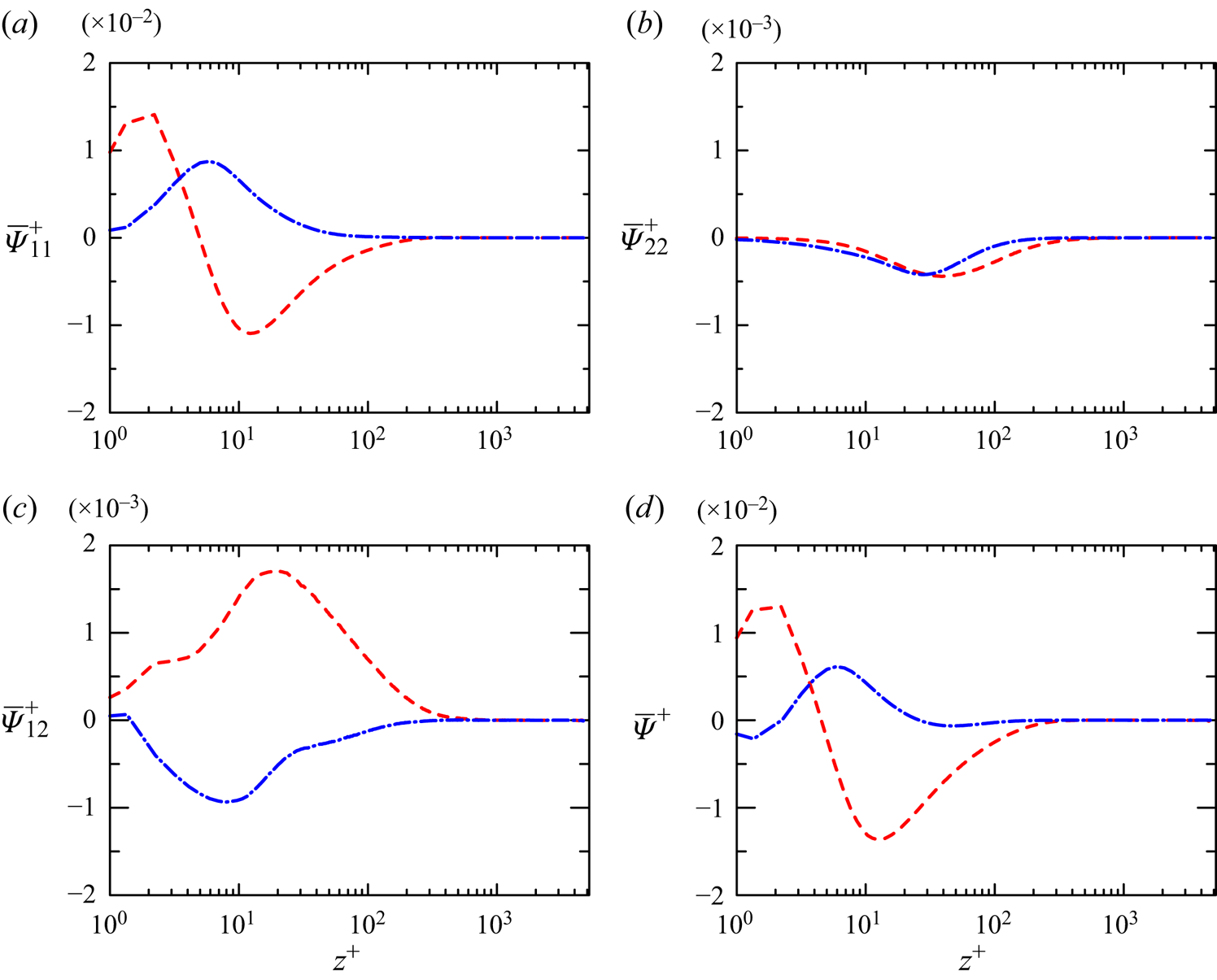
Figure 5 shows the particle source terms $\bar {\varPsi }_{11}^+$ ($\overline {u'u'}$ budget), $\bar {\varPsi }_{22}^+$ ($\overline {w'w'}$ budget), $\bar {\varPsi }_{12}^+$ ($\overline {u'w'}$ budget) and $\bar {\varPsi }^+$ (TKE budget). The feedback terms are maximum near the wall where the shear rate is the strongest, which generates the major evident signature of the turbulence modulation by particles. $\bar {\varPsi }_{11}^+$ is always positive (source) for the low-$St$ case, meaning that the streamwise velocity fluctuations are forced by the Stokes drag (Gualtieri et al. Reference Gualtieri, Picano, Sardina and Casciola2013). For the high-$St$ case, $\bar {\varPsi }_{11}^+$ is almost always negative (sink) except for $z^+<5$. Here $\bar {\varPsi }^+$ shows similar trend as $\bar {\varPsi }_{11}^+$. This is consistent with the idea that heavy, inertial particles inhibit strong turbulent fluctuations by simply acting as obstacles in the viscous and buffer layers (Richter Reference Richter2015). We find that $\bar {\varPsi }_{22}^+$ is always negative (sink), meaning that Stokes drag intercepts momentum from the fluid turbulence and depletes the velocity fluctuations in the wall-normal direction. The $St$ dependence of $\bar {\varPsi }_{11}^+$ and $\bar {\varPsi }_{22}^+$ is similar to the DNS results of Wang & Richter (Reference Wang and Richter2020). We find that $\bar {\varPsi }_{12}^+$ is always negative (sink) for low $St$, but positive (source) for high $St$, which is actually opposite to $\bar {\varPsi }_{11}^+$. It can be noted that the particle contributions to both the Reynolds stress and TKE budgets tend to vanish for $z^+ \ge 300$. As argued in Richter (Reference Richter2015) and Wang & Richter (Reference Wang and Richter2019), however, it is important to recognise that the direct contribution $\varPsi$ is not the only mechanism by which particles can modify turbulence.

Figure 5.

Profiles of the particle feedback terms to Reynolds stress budget: (a) particle sources to the $\overline {u'u'}$ budget, $\bar {\varPsi }_{11}^+$; (b) particle sources to the $\overline {w'w'}$ budget, $\bar {\varPsi }_{22}^+$; (c) particle sources to the $\overline {u'w'}$ budget, $\bar {\varPsi }_{12}^+$; (d) particle contributions to the TKE budget, $\bar {\varPsi }^+$. Curves: – – – –, high-$St$ case (C1); —$\cdot$—, low-$St$ case (C2). All terms are normalised by $u_{\tau }^3 / \delta _{\nu }$.

Owing to the slip velocity induced by particle inertia, the particles working on the fluid not only act as a direct source/sink in the Reynolds stress budgets, but also transfer energy between fluid and particles. The imbalance between the energy transferred from the fluid to the particles and the energy received from the particles to the fluid reflects energy dissipation, which may help describe the mechanism of drag reduction in particle-laden flow. The time rate of the work done by the local fluid to a particle $W_{p}$, the work done by a particle on the local fluid $W_{f}$, and the particle dissipation $\epsilon$ are expressed as (Zhao et al. Reference Zhao, Andersson and Gillissen2013)

(3.3) \begin{equation} \left.\begin{gathered} W_{p} =6 {\rm \pi}\mu a(u_{f,i}-u_{p,i}) u_{p,i}, \\ W_{f} ={-}6 {\rm \pi}\mu a(u_{f,i}-u_{p,i}) u_{f,i}, \\ \epsilon=W_{p}+W_{f} ={-}6 {\rm \pi}\mu a(u_{f,i}-u_{p,i})(u_{f,i}-u_{p,i}), \end{gathered}\right\} \end{equation}

where $a$ is the particle radius, and $u_{p,i}$ and $u_{f,i}$ are the particle velocity and the fluid velocity seen by the particle, respectively.

Figure 6 shows the mean power transferred between fluid and particles. Due to larger magnitudes of slip velocities at high $St$, i.e. $\Delta \bar {u}^+$ and $\Delta \bar {w}^+$ (see figure 3), the intensity of energy transfer and dissipation at high $St$ is much stronger than that at low $St$. For the low-$St$ case, the particles exert work on the local fluid ($\bar {W}_{p}<0$, $\bar {W}_{f}>0$) for $z^+ < 20$, above which the energy transfer mechanism is negligible. For the high-$St$ case, the particles exert work on the local fluid for $z^+ < 500$, whereas receive energy from the fluid ($\bar {W}_{p}>0$, $\bar {W}_{f}<0$) for $z^+ > 20$. The peak locations of $\bar {W}_{p}$ and $\bar {W}_{f}$ are consistent with the streamwise slip velocity (figure 3). The non-zero $\bar {\epsilon }$ denotes extra energy dissipation caused by particles. The particle dissipation is most pronounced in the near-wall region but retain an appreciable level below the wake region for the high-$St$ case. The overall trend of $W_{p}$, $W_{f}$ and $\epsilon$ is qualitatively similar to Zhao et al. (Reference Zhao, Andersson and Gillissen2013), although their analysis is restricted to heavy particles at $Re_{\tau } =180$. Zhao et al. (Reference Zhao, Andersson and Gillissen2013) reported a transient location, i.e. $z^+ =36$, above which that particles receive energy from the fluid ($\bar {W}_{p}>0$, $\bar {W}_{f}<0$). The present DNS indicates that the transient location is not only a function of the Reynolds number, but also dependent on the Stokes number.

Figure 6.

Profiles of the mean power transferred between fluid and particles: (a) from the fluid to the particle, $\bar {W}_{p}^+$; (b) from the particle to the fluid, $\bar {W}_{f}^+$; (c) particle dissipation, $\bar {\epsilon }^+$. Curves: – – – –, high-$St$ case (C1); —$\cdot$—, low-$St$ case (C2). The mean power is normalised by $6{\rm \pi} \mu a u_{\tau }^2$.

3.3. Spectral analysis

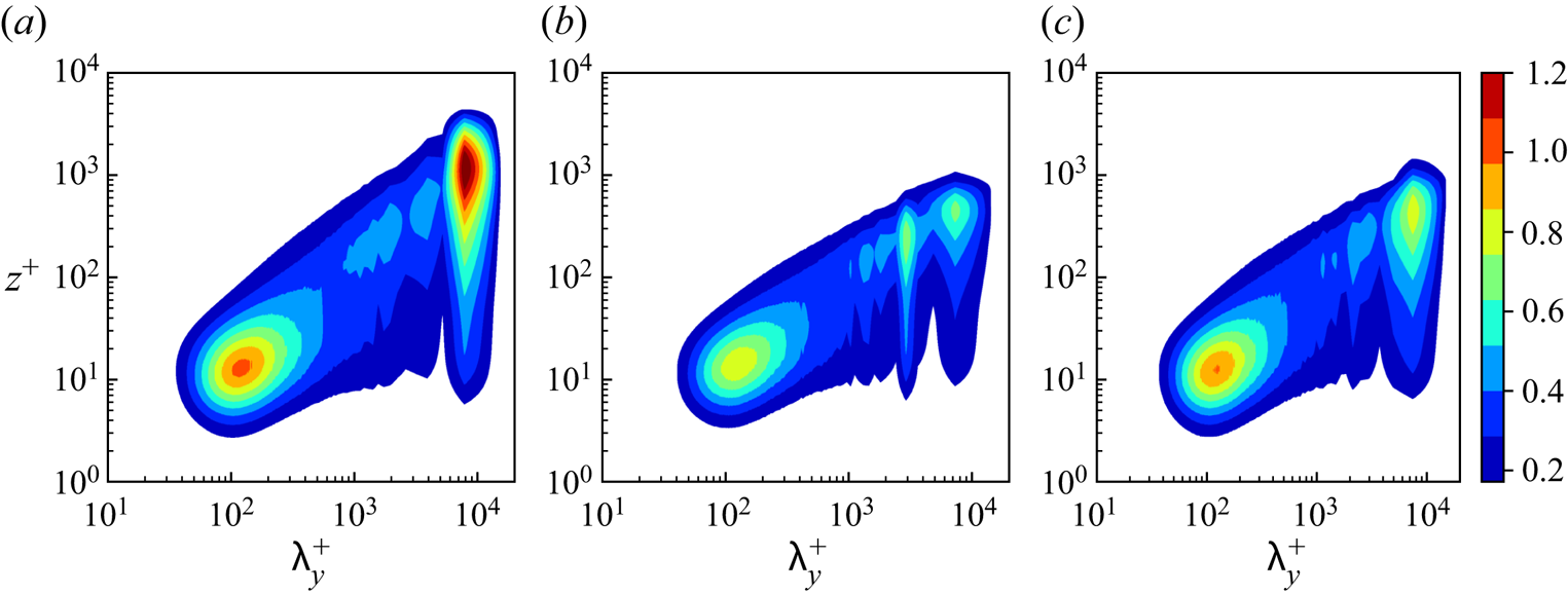
High-Reynolds-number wall-bounded turbulence is characterised by scale separations between the near-wall and outer-layer turbulence, which is at the heart of all scaling theories (McKeon & Sreenivasan Reference McKeon and Sreenivasan2007). This separation of scales can be seen in the one-dimensional velocity spectra. Figure 7 shows the wavenumber-premultiplied one-dimensional $u$-spectra $k_y \varPhi _{u'u'} (k_y)/u^2_{\tau }$, where $\varPhi _{u'u'} (k_y) = \langle \hat {u}'(k_y) \hat {u}^{* \prime }(k_y) \rangle$ ($\hat {u}'$ is the Fourier coefficient of $u'$), as functions of spanwise wavelength $\lambda ^+_y$. For the unladen case, the energy spectral density of $u$ in the spanwise direction contains two distinct peaks, i.e. one at $\lambda ^+_y =117$, $z^+=13$, and the other at $\lambda ^+_y =7762$, $z^+=1122$. Such distinct peaks have previously been observed in high-Reynolds-number experimental (Hutchins & Marusic Reference Hutchins and Marusic2007; Marusic et al. Reference Marusic, McKeon, Monkewitz, Nagib, Smits and Sreenivasan2010; Smits et al. Reference Smits, McKeon and Marusic2011) and DNS investigations (Lee & Moser Reference Lee and Moser2015; Yamamoto & Tsuji Reference Yamamoto and Tsuji2018). In DNS of particle-laden open channel flows ($Re_{\tau }=550, 950, 2.42 \le St^+ \le 908$), Wang & Richter (Reference Wang and Richter2019) found that particles weaken LSMs in the inner layer whereas they enhance VLSMs in the outer layer. At the higher Reynolds number of the present simulations, however, both LSMs and VLSMs are generally weakened in the inner and outer layers, as shown in figure 7. The peaks in the spectra located at $\lambda _{y}^{+} \approx 150$ and $\lambda _{y}^{+} \approx 10{\,}000$ are significantly reduced in magnitude (particularly the VLSM peak), whereas there is a small region of energy enhancement around $\lambda _{y}^{+} \approx 3000$ for the high-$St$ particles. The vertical range containing VLSMs is also reduced by the particles, especially for the high-$St$ case. The weakened strength increases with increased $St$, and the contribution from VLSMs forms a bimodal spanwise spectrum in the outer layer for the high-$St$ case: this feature is muted in the low-$St$ case.

Figure 7.

Wavenumber-premultiplied one-dimensional $u$-spectra $k_y \varPhi _{u'u'} (k_y)/u^2_{\tau }$ as functions of spanwise wavelength and wall-normal direction: (a) unladen case (C0), (b) high-$St$ case (C1) and (c) low-$St$ case (C2). The values are scaled by the maximum value in the inner layer of the unladen flow.

In Wang & Richter (Reference Wang and Richter2019), it was demonstrated that the particles tended to enhance VLSM energy at $Re_{\tau } = 550$ and $Re_{\tau } = 950$, and that this was a non-monotonic function of Stokes number. The DNS showed that VLSM energy was enhanced at two different $St$, but through two different mechanisms: direct interaction between particles and VLSM structures at high $St$, and indirect, nonlinear interactions between particles, near-wall LSM and VLSM structures at low $St$. In the present simulations, however, figure 7 indicates that, at least for the two $St$ considered presently, the peak LSM and VLSM energy is damped, and that the behaviour observed by Wang & Richter (Reference Wang and Richter2019) is somehow not present. Although this discrepancy may be simply due to the fact that the previous Reynolds numbers were only just entering the asymptotic regime for wall-bounded turbulence and therefore the VLSMs are only emergent (Smits et al. Reference Smits, McKeon and Marusic2011), we turn to the spectral signature of energy production to understand the mechanism behind the changes in LSM and VLSM energy observed in figure 7.

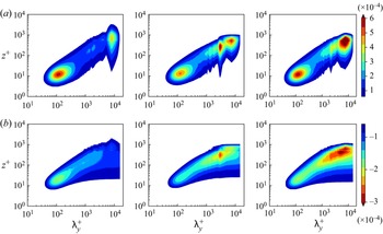
In spectral space, the modulation of LSMs and VLSMs by particles is at least partially related to the direct influence on velocity fluctuations, which, in turn, can modify the production of TKE and Reynolds shear stress (see figure 5 and the discussion in Wang & Richter Reference Wang and Richter2019). This is demonstrated in figure 8, where we present the $\overline {u'u'}$ spectral production term $\hat {P}_{11}=-\langle \hat {u}^{\prime } (k_{y}, z) \hat {w}^{\prime *} (k_{y}, z) \rangle \mathrm {d} \bar {u} / \mathrm {d} z$, as well as the $\overline {u'w'}$ spectral production term $\hat {P}_{12}=-\langle \hat {w}^{\prime } (k_{y}, z) \hat {w}^{\prime *} (k_{y}, z) \rangle \mathrm {d} \bar {u} / \mathrm {d} z$, as functions of spanwise wavelength $\lambda ^+_y$. Throughout the wall-normal direction, $\hat {P}_{11}$ is positive whereas $\hat {P}_{12}$ is negative. Comparing the premultiplied $u$-spectrum (figure 7) and $\hat {P}_{11}$-spectrum, we find that they have a similar overall shape. In the inner layer associated with LSMs, the $\overline {u'u'}$ production term $\hat {P}_{11}$ is weakened by particles, but enhanced in the outer layer associated with VLSMs. This means that in the inner layer, the presence of particles reduces the production of $\overline {u'u'}$ compared with the unladen case, whereas in the outer layer they act to promote VLSM energy. Indeed, the peak in $\hat {P}_{11}$ near $\lambda _{y}^{+} \approx 3000$ for the high-$St$ case seems to correspond directly to the local maximum of TKE observed in figure 7(b) – at these wavelengths at the large Stokes numbers, energy is being directly used to promote LSMs at a very narrow wavenumber band. Thus, the particles would seem to act as a direct source of streamwise kinetic energy at the VLSM scale based only on $\hat {P}_{11}$.

Figure 8.

Spectral production contribution to the streamwise TKE budget and Reynolds shear stress budget: (a) $\hat {P}_{11}$, (b) $\hat {P}_{12}$, normalised by $u^3_{\tau }/{\delta _v}$. Panels from left to right correspond to the unladen case (C0), high-$St$ case (C1) and low-$St$ case (C2), respectively.

Figure 7, however, showed a considerable decrease in VLSM energy centred around $\lambda _{y}^{+} \approx 10{\,}000$. In figure 5(b), it is observed that the particles simultaneously act as a sink in the Reynolds shear stress budget at the VLSM scale. This is evident in figure 1(e), and indicates a severe reduction of TKE shear production. This reduction of energy production ultimately wins the competition for decreasing the energy contained in the VLSM range, over the direct contribution $\hat {P}_{11}$ from the particles. Figure 5 also shows that the primary effect of $St$ is to alter the magnitude of the impacts on $\hat {P}_{11}$ and $\hat {P}_{12}$ (similar to the energy in figure 7). This is in contrast to Wang & Richter (Reference Wang and Richter2019), who observed qualitatively different patterns in $\hat {P}_{11}$ and $\hat {P}_{12}$ for the low- and high-Stokes number cases (see their figure 12). The present results at the higher Reynolds number would seem to suggest that the results of Wang & Richter (Reference Wang and Richter2019) may unique to Reynolds numbers near the cusp of being considered asymptotic in the outer layer, but additional simulations at a wider range of $St$ at $Re_{\tau } = 5186$ would be needed to confirm this. It is worth noting that at much larger Reynolds numbers in the atmospheric surface layer ($Re_{\tau } = O(10^{6})$), Wang, Gu & Zheng (Reference Wang, Gu and Zheng2020a) and Liu, He & Zheng (Reference Liu, He and Zheng2021) have observed that the effect of airborne sand/dust is to increase the energy contained in the VLSM range as compared with dust-free conditions.

3.4. Instantaneous flow structure and particle behaviour

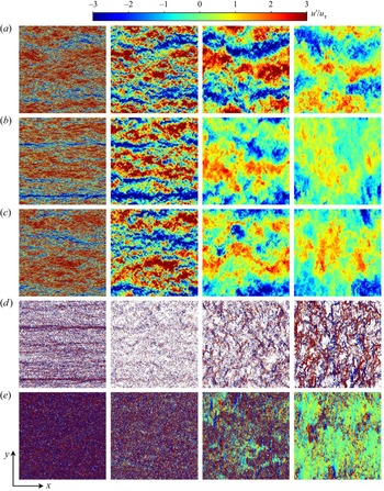
In order to visualise the turbulent structures associated with local enhancements of particle population, figure 9 shows the instantaneous streamwise velocity fluctuation and the corresponding snapshots of particle locations at four $x$–$y$ slabs, i.e. 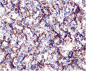$z^+ = 13, 270, 1122, 3630$, where $z^+ = 13$ and $z^+ = 1122$ correspond to the peak locations of the premultiplied $u$-spectrum for the unladen case; $z^+ = 270$ corresponds to the outer peak locations of the premultiplied $u$-spectrum for the laden case; $z^+ = 3630$ corresponds to the wake region. Particles accumulating in the inner-flow low-speed streaks can be observed for the high-$St$ case (figure 9b,d), whereas low-inertia particles tend to distribute homogeneously in wall-normal planes (figure 9e). This is similar to many other studies (Pan & Banerjee Reference Pan and Banerjee1996; Marchioli & Soldati Reference Marchioli and Soldati2002; Wang & Richter Reference Wang and Richter2019).

Figure 9.

Instantaneous streamwise velocity fluctuation $u'/u_{\tau }$ for the (a) unladen case (C0), (b) high-$St$ case (C1), (c) low-$St$ case (C2) and the corresponding instantaneous snapshots of particle locations for (d) high-$St$ case (C1), $(e)$ low-$St$ case (C2) in four $x$–$y$ planes (panels from left to right: $z^+ = 13$, $z^+ = 270$, $z^+ = 1122$, $z^+ = 3630$). The particles are coloured by the instantaneous streamwise slip velocity $\Delta u^+ = (u-u_p)/u_{\tau }$, which shares the colourmap of $u'/u_{\tau }$ within $[-0.03,0.03]$. For better visualisations, all the figures are stretched in the $y$-direction.

To characterise the anisotropic clustering of the particles in the ensemble-averaged sense, we employ the angular distribution functions (ADFs) (Gualtieri, Picano & Casciola Reference Gualtieri, Picano and Casciola2009). Here we consider the two-dimensional angular distribution function, $\operatorname {ADF}(r, \theta )$, defined as

(3.4) \begin{equation} \operatorname{ADF}(r, \theta)=\frac{\displaystyle\sum_{i=1}^{n_{p}} \delta N_{i}(r, \theta)/ (\delta r \delta \theta r n_{p})}{N /(L_{x} L_{y})},\quad 0 \leqslant \theta \leqslant {\rm \pi}/ 2, \end{equation}

where particles are collected from a slab with thickness of $2d$; $\delta N_{i}(r, \theta )$ is the particle number in a sector between $r-\delta r/2$ and $r + \delta r/2$ in the radial direction and $r-\delta \theta /2$ and $r + \delta \theta /2$ in the angular direction from the centre of particle $i$; $\theta =0$ and $\theta = {\rm \pi}/2$ correspond to the spanwise and streamwise directions, respectively. Following Wang & Richter (Reference Wang and Richter2020), we set $\delta r = 0.008h$ ($\delta r^+ \approx 40$) and $\delta \theta = 0.025 {\rm \pi}$ to compute $\operatorname {ADF}(r, \theta )$. The mean value is from the average of $n_p$ particles from multiple snapshots in time. Finally, the distribution functions are normalised by the surface average particle number in the $x$–$y$ plane ($N/L_xL_y$ representing a randomly distributed particle number density, where $N$ denotes the mean particle number of the two-dimensional $x$–$y$ slab taken in the wall-normal direction). Periodic boundary conditions are used for particles in the streamwise and spanwise directions.

Figure 10 shows $\operatorname {ADF}(r, \theta )$ in the spanwise ($\theta =0$) and streamwise ($\theta = {\rm \pi}/2$) directions at two typical wall-normal heights: $z^+ = 13$ (inner layer) and $z^+ = 1122$ (outer layer). For the high-$St$ case, the particle density from a reference particle in the streamwise direction is higher than in the spanwise direction. For the low-$St$ case, the particles tend to distribute homogeneously without obvious clustering behaviour, consistent with figure 9.

Figure 10.

The (a) spanwise and (b) streamwise ADF of particles in the $x$–$y$ slabs with thickness of $2d$ at two wall-normal heights: $z^+ = 13$ (left), $z^+ = 1122$ (right). Curves: – – – –, high-$St$ case (C1); —$\cdot$—, low-$St$ case (C2).

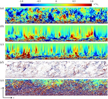
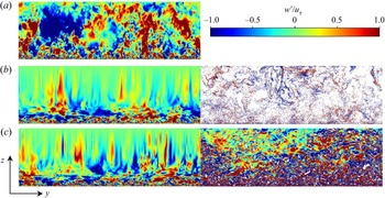
Figures 11 and 12 show the instantaneous wall-normal velocity fluctuation and the corresponding snapshots of particle locations in the $x$–$z$ and $y$–$z$ planes, respectively. In the near-wall region ($z/h \le 0.2$), we can observe inclined structures that high-speed regions alternate with low-speed regions, which is similar to the observation by Zhang, Hu & Zheng (Reference Zhang, Hu and Zheng2018) in the atmospheric boundary layer with suspended dust. In the wake region ($z/h>0.2$), vertical structures can be observed in the laden cases, i.e. regions of positive vertical velocity fluctuations are flanked on either side by regions of negative vertical velocity fluctuations in both the streamwise and spanwise directions. The size of these vertical structures are larger due to the particle–turbulence interaction, compared with the unladen case. The low-inertia particles act as scalar tracers near the free surface, in accordance with the observations in figure 9.

Figure 11.

Instantaneous wall-normal velocity fluctuation $w'/u_{\tau }$ for the (a) unladen case (C0), (b) high-$St$ case (C1), (c) low-$St$ case (C2) and the corresponding instantaneous snapshots of particle locations for (d) high-$St$ case (C1), (e) low-$St$ case (C2) in the $x$–$z$ plane. The particles are coloured by the instantaneous wall-normal slip velocity $\Delta w^+ = (w-w_p)/u_{\tau }$, which shares the colourmap of $w'/u_{\tau }$ within $[-0.01,0.01]$.

Figure 12.

Instantaneous wall-normal velocity fluctuation $w'/u_{\tau }$ for the (a) unladen case (C0), (b) high-$St$ case (C1), (c) low-$St$ case (C2) and the corresponding instantaneous snapshots of particle locations (right) in the $y$–$z$ plane. The particles are coloured by the instantaneous wall-normal slip velocity $\Delta w^+ = (w-w_p)/u_{\tau }$, which shares the colourmap of $w'/u_{\tau }$ within $[-0.01,0.01]$.

3.5. Correlation analysis

The spatial two-point correlations of streamwise velocity fluctuations are utilised to explore the effect of particles on the average spatial structure of the flow. The streamwise two-point autocorrelations of the streamwise velocity fluctuations at different reference planes are computed as

(3.5)\begin{equation} R_{uu} (\Delta x, z_r)= \frac{\overline{ \langle u'(x+\Delta x,y,z) u'(x,y,z_r) \rangle} }{\langle u_{rms}'(x+\Delta x,y,z) \rangle \langle u_{rms}'(x,y,z_r) \rangle}, \end{equation}

where the brackets denotes an averaging operation over the homogenous horizontal plane.

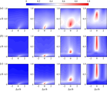
Figure 13 shows the contour plots of $R_{uu} (\Delta x, z_r)$ for both laden and unladen cases, which are computed at four reference planes, as illustrated in figure 9. The high-correlation region near the wall highlights the inclined VLSMs, as noted in figures 11 and 12, which is similar to the atmospheric surface layer at $Re_{\tau } \sim O(10^6)$ (Wang et al. Reference Wang, Gu and Zheng2020a). However, the particles tend to decrease the inclination angles of VLSMs, which is opposite to the observations by Wang et al. (Reference Wang, Gu and Zheng2020a). The vertical structures are also observed in the wake region ($z/h>0.2$) for the laden cases. In the inner layer associated with LSMs ($z_r^+ =13$), the LSMs in the unladen case have stronger correlations with the VLSMs of the outer region compared with the laden case, which indicates stronger interactions between LSMs and VLSMs. In the wake region ($z_r^+ =1122$), the particles weaken the streamwise correlation, and the weakened strength is even stronger for the high-$St$ case, consistent with the $u$-spectrum shown in figure 7. However, this behaviour is opposite at $z_r^+ =3630$ for the laden cases, i.e. the streamwise correlation of high-$St$ case is slightly stronger than the low-$St$ case.

Figure 13.

Contours of $R_{uu}(\Delta x,z_r)$ for the (a) unladen case (C0), (b) high-$St$ case (C1), (c) low-$St$ case (C2) at four $z_r$ locations $z_r^+ = 13$, $z_r^+ = 270$, $z_r^+ = 1122$ and $z_r^+ = 3630$.

A better understanding of the growth of coherent structures with wall distance can be gained from $R_{uu} (\Delta x, \Delta y)$, computed as

(3.6)\begin{equation} R_{uu} (\Delta x, \Delta y)= \frac{\overline{ \langle u'(x,y) u'(x+\Delta x,y+\Delta y) \rangle}}{\langle u_{rms}'(x,y) \rangle \langle u_{rms}'(x+\Delta x,y+\Delta y) \rangle}. \end{equation}

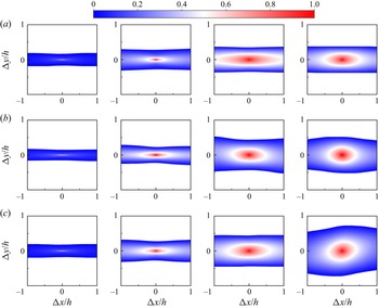
Figure 14 shows the contour plots of $R_{uu} (\Delta x, \Delta y)$ at four reference planes (same as figure 13). Here only positive correlated regions ($R_{uu} (\Delta x, \Delta y) \ge 0.05$) are shown, where the threshold value of $0.05$ indicates the coherent structure edge according to Hutchins & Marusic (Reference Hutchins and Marusic2007). Positive correlation regions are flanked by anti-correlated behaviour (not shown) in the spanwise direction, reflecting the spanwise striping of high- and low-momentum regions as noted in figure 9 (Hutchins & Marusic Reference Hutchins and Marusic2007). For all cases, the spanwise width of coherent structures increases with wall distance, and the growth rate is larger in the log region whereas smaller in the wake region, which is in consistent with the observation by Monty et al. (Reference Monty, Stewart, Williams and Chong2007). The spanwise scale in the log region is similar, but the particles widen these scales in the wake region, particularly for the low-$St$ case (see also figure 9). The streamwise size of the VLSMs is largest for the unladen case, and the presence of particles shortens their extent, especially for high $St$, which indicates the weakening effects of particles as noted in figure 7.

Figure 14.

Contours of $R_{uu}(\Delta x, \Delta y)$ for the (a) unladen case (C0), (b) high-$St$ case (C1), (c) low-$St$ case (C2) in four $x$–$y$ planes $z^+ = 13$, $z^+ = 270$, $z^+ = 1122$ and $z^+ = 3630$. Here $R_{uu} < 0.05$ are cut off.

3.6. Alignment of the vorticity and the strain-rate tensor

In order to gain a better insight into the dynamics at small scales, we analyse the alignment of the vorticity vector, ${\boldsymbol {\omega }}$ with the eigenvectors of the strain-rate tensor $s_{ij}$, whose associated eigenvalues are $\lambda _1 < \lambda _2 < \lambda _3$, also referred to as the principal strain rates. Due to incompressibility, the trace of $s_{ij}$ must be zero, which results in $\lambda _1 < 0$ and $\lambda _3 > 0$. The eigenvectors associated with $\lambda _1$, $\lambda _2$ and $\lambda _3$ represent the principal compressing, intermediate and stretching stress directions, respectively. The orientation of the vorticity vector ${\boldsymbol {\omega }}$ with the principal eigenvectors is commonly expressed by the cosine of the angle, i.e. $\cos (\boldsymbol {\omega }, \lambda _i) (i=1,2,3)$, which is determined from the inner products of vectors.

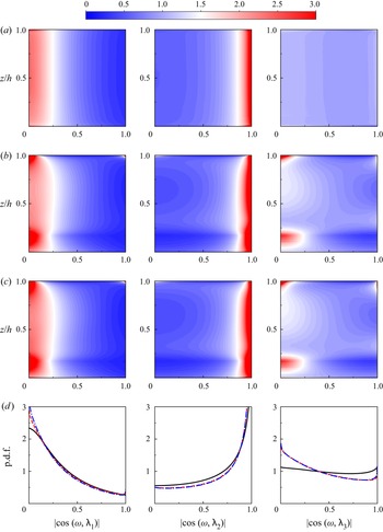
Figure 15 shows the probability density functions (p.d.f.s) of $\cos (\boldsymbol {\omega }, \lambda _i)$. The vorticity displays a preferential alignment with the intermediate eigenvector, showing as an increased probability of $| \cos (\omega, \lambda _2) | =1$, for both laden and unladen cases. This is in agreement with previous observations in isotropic turbulence (Ashurst et al. Reference Ashurst, Kerstein, Kerr and Gibson1987), free and contracted shear flow (Mullin & Dahm Reference Mullin and Dahm2006; Mugundhan et al. Reference Mugundhan, Pugazenthi, Speirs, Samtaney and Thoroddsen2020), turbulent boundary layer flow (Elsinga & Marusic Reference Elsinga and Marusic2010) and turbulent channel flow (Lozano-Durán, Holzner & Jiménez Reference Lozano-Durán, Holzner and Jiménez2016, $Re_{\tau }=932$). It should be noted that these references only include the spatially averaged p.d.f.s, which lack the detailed structures along the wall-normal direction. For the unladen case, the p.d.f.s of $\cos (\boldsymbol {\omega }, \lambda _i)$ are almost uniform in the $z$-direction, but for the particle-laden cases, the alignment of ${\boldsymbol {\omega }}$ with $\lambda _2$ intensifies in the near-wall and free-surface regions, showing increased probability of $| \cos (\omega, \lambda _1) | =0$ and $| \cos (\omega, \lambda _3) | =0$. The wall-normal averaged p.d.f.s of $| \cos (\omega, \lambda _2) |$ (see figure 15d) also show this difference, i.e. slightly higher p.d.f.s close to $| \cos (\omega, \lambda _2) | =1$. Furthermore, the vorticity is mostly oriented normal to the compressing eigenvector, and particles slightly intensify this. The particle effects become apparent for the stretching eigenvector, more of which are perpendicular to the vorticity. Overall, the alignment preference seems to be independent of the particle Stokes number.

Figure 15.

Probability density functions of the cosine of the angle between the vorticity vector and the three eigenvectors of the strain-rate tensor (panels from left to right: compressing vector, intermediate vector and stretching vector): (a) unladen case (C0), (b) high-$St$ case (C1), (c) low-$St$ case (C2) and (d) wall-normal averaged p.d.f.s. Curves: ——, unladen case; – – – –, high-$St$ case; —$\cdot$—, low-$St$ case.

These findings are essential particularly in the context of LES and the development of subgrid-scale (SGS) model, especially the structure-based SGS models (Meneveau & Katz Reference Meneveau and Katz2000). One such physical model is the stretched-spiral vortex SGS model originally developed by Misra & Pullin (Reference Misra and Pullin1997). They introduced a stretched vortex to model the SGS effect for LES in the following way: embedded within each computational cell, there exists a superposition of stretched vortices, each having orientation taken from a p.d.f. It is essentially a local alignment model, which assumes a fraction of the local dominant subgrid structures tend to align with the stretching eigenvector and the remainder align with the intermediate eigenvector. Chung & Pullin (Reference Chung and Pullin2009) orients the SGS vortices along the stretching eigenvector, and this idea has been applied successfully in LES of wall-bounded turbulent flows: turbulent channel flow (Chung & Pullin Reference Chung and Pullin2009; Gao, Cheng & Samtaney Reference Gao, Cheng and Samtaney2020), turbulent boundary layer flow (Inoue & Pullin Reference Inoue and Pullin2011) and airfoil flow (Gao et al. Reference Gao, Zhang, Cheng and Samtaney2019). The alignment of the vortical structures in particle-laden flows is, in a sense, a validation of the assumption of orientation along stretching eigenvectors in the stretched-spiral vortex SGS model. Our DNS results in the particle-laden open channel flow may serve as a guide to other SGS models that rely on the vortex alignment in LES of particle-laden flows.