


1 Introduction
Turbulent flows in rotating systems are of great practical importance in industrial applications involving turbomachinery. In such flows, system rotation introduces additional body forces (i.e. Coriolis and centrifugal forces) arising from the non-inertial reference frame. These additional forces are known to have a substantial effect on turbulent flow statistics and structure.
(a) Schematic geometry of SR in a turbulent channel flow. (b) Conceptual illustration of the resolvent analysis.

The simplest flow in this category is a fully developed channel flow under spanwise rotation (SR), i.e. where the entire system rotates around the spanwise axis at the channel centreline. This particular model flow has been studied extensively through both laboratory experiments and numerical simulations. The pioneering experiments pursued by Johnston, Halleen & Lezius (Reference Johnston, Halleen and Lezius1972) and direct numerical simulations (DNS) carried out by Kristoffersen & Andersson (Reference Kristoffersen and Andersson1993) showed that SR induces a number of important changes relative to canonical turbulent channel flows. For example, the streamwise mean velocity profile becomes asymmetric across the channel centreline. In particular, a constant linear slope appears in the mean velocity at the channel centreline, with a shear rate close to twice the angular velocity of the system rotation. In other words, the absolute mean vorticity in this region reduces to almost zero. Further, turbulence intensities are enhanced on the pressure side where the rotation is in the same direction as the mean flow, and suppressed on the suction side where the rotation is counter to the mean flow direction (see figure 1 a). Finally, large-scale roll cells emerge in rotating channel flows due to Taylor–Görtler instabilities, and these roll cells move towards the pressure side with increasing rotation rates.
Building on these early studies, Wu & Kasagi (Reference Wu and Kasagi2004) investigated, using DNS, the effect of arbitrary system rotation in turbulent channel flows by combining streamwise, spanwise and wall-normal rotation, and found that SR has the dominant influence. More recently, Grundestam, Wallin & Johansson (Reference Grundestam, Wallin and Johansson2008) have carried out DNS at much higher rotation rates compared to those used by Kristoffersen & Andersson (Reference Kristoffersen and Andersson1993). These simulations show that, while turbulence is initially enhanced on the pressure side due to system rotation, a further increase in rotation rate leads to turbulence suppression on the pressure side. Moreover, complete flow laminarization occurs at a rotation number of
 $\mathit{Ro}_{\unicode[STIX]{x1D70F}}=2\unicode[STIX]{x1D6FA}h/u_{\unicode[STIX]{x1D70F}}\leqslant 180$
for friction Reynolds number
 $\mathit{Re}_{\unicode[STIX]{x1D70F}}=u_{\unicode[STIX]{x1D70F}}h/\unicode[STIX]{x1D708}=180$
. Note that
 $\unicode[STIX]{x1D6FA}$
is the system rotation rate,
 $u_{\unicode[STIX]{x1D70F}}$
is the global friction velocity in the channel,
 $h$
is the channel half-height and
 $\unicode[STIX]{x1D708}$
is the kinematic viscosity. Subsequent linear analyses conducted by Wallin, Grudestam & Johansson (Reference Wallin, Grundestam and Johansson2013) show results consistent with the DNS of Grundestam et al. (Reference Grundestam, Wallin and Johansson2008), and indicate that the critical rotation number for relaminarization is a monotonic function of Reynolds number. The success of these analyses also suggests that laminarization in rapidly rotating turbulent channel flows is dominated by linear mechanisms.
In addition to the studies described above, Yang & Wu (Reference Yang and Wu2012) and Xia, Shi & Chen (Reference Xia, Shi and Chen2016) have also performed DNS of rotating channel flow at
 $\mathit{Re}_{\unicode[STIX]{x1D70F}}=180$
. Based on a helical wave decomposition, Yang & Wu (Reference Yang and Wu2012) showed that the fluctuation energy is concentrated in large-scale modes for slow SR (
 $\mathit{Ro}_{\unicode[STIX]{x1D70F}}<2.5$
), but shifts towards smaller scales as the rotation number increases (
 $\mathit{Ro}_{\unicode[STIX]{x1D70F}}>2.5$
). For
 $\mathit{Ro}_{\unicode[STIX]{x1D70F}}>20$
, the wavenumber carrying maximum energy is larger than that in the non-rotating channel. Xia et al. (Reference Xia, Shi and Chen2016) conducted DNS over a wider range of rotation number compared to Kristoffersen & Andersson (Reference Kristoffersen and Andersson1993) and Grundestam et al. (Reference Grundestam, Wallin and Johansson2008), providing more detailed insight into the variation of turbulence statistics with rotation rate.
In their latest work, Brethouwer (Reference Brethouwer2017) investigated the effect of SR on channel flow at constant bulk Reynolds number
 $\mathit{Re}_{b}$
in the range 3000–31 600. The friction Reynolds number
 $\mathit{Re}_{\unicode[STIX]{x1D70F}}$
was allowed to vary with rotation rate. This is in contrast to the studies mentioned above, which were all carried out for a constant pressure gradient (i.e. fixed
 $\mathit{Re}_{\unicode[STIX]{x1D70F}}$
). Two-point correlations obtained by Brethouwer (Reference Brethouwer2017) indicated that the roll cell-like structures that emerge under SR varied considerably with
 $\mathit{Re}_{b}$
.
The present work seeks to provide further insight into the mechanisms leading to the changes to turbulent flow structure and statistics described above by conducting resolvent analysis (McKeon & Sharma Reference McKeon and Sharma2010) for turbulent channel flow under SR. We consider the effect of SR on turbulent flow structures on the unstable pressure side of the channel for a range of rotation rates at both low and high Reynolds number. Specifically, we generate resolvent-based predictions at
 $\mathit{Re}_{\unicode[STIX]{x1D70F}}=180$
, as considered in previous DNS, and at
 $\mathit{Re}_{\unicode[STIX]{x1D70F}}=2000$
, which corresponds roughly to conditions under which the so-called very-large-scale motions (VLSMs) or superstructures become important. In addition to allowing an exploration at high Reynolds number, resolvent analysis also allows us to decouple the two different effects that can influence turbulent flow structure and statistics: the changes in the mean profile arising from system rotation and the introduction of additional body forces in the governing equations. Further, this paper also serves to evaluate whether the resolvent formulation, which has previously been shown to generate useful predictions for flows with wall-based active control (Luhar, Sharma & McKeon Reference Luhar, Sharma and McKeon2014; Nakashima, Fukagata & Luhar Reference Nakashima, Fukagata and Luhar2017), can account for flows in which the external forcing appears as a distributed body force (e.g. the Coriolis term in turbulent channel flows with SR).
The remainder of this paper is organized as follows. In § 2, we review the flow configuration and governing equations (§ 2.1) and the theoretical formulation for resolvent analysis (§ 2.2), and provide details of numerical implementation (§ 2.3). In § 3, we consider the effect of SR on turbulent flow structures on the pressure side at
 $\mathit{Re}_{\unicode[STIX]{x1D70F}}=180$
(§ 3.1) and
 $\mathit{Re}_{\unicode[STIX]{x1D70F}}=2000$
(§ 3.2), focusing in particular on how the effect of SR is distributed across spectral space. We provide further discussion of scale effects and Reynolds number effects in § 3.3, and present concluding remarks in § 4.
2 Analysis method
2.1 Governing equations and flow configuration
As shown schematically in figure 1(a), we consider a fully developed turbulent flow between two infinite parallel plates under SR with constant angular velocity
 $\unicode[STIX]{x1D734}=[0~0~\unicode[STIX]{x1D6FA}]^{\text{T}}$
. The governing Navier–Stokes equations and continuity constraint for this system can be expressed as
 $$\begin{eqnarray}\unicode[STIX]{x1D735}\boldsymbol{\cdot }\boldsymbol{u}=0,\quad \frac{\unicode[STIX]{x2202}\boldsymbol{u}}{\unicode[STIX]{x2202}t}=-\unicode[STIX]{x1D735}p-\boldsymbol{u}\boldsymbol{\cdot }\unicode[STIX]{x1D735}\boldsymbol{u}+\frac{1}{\mathit{Re}_{\unicode[STIX]{x1D70F}}}\unicode[STIX]{x1D6FB}^{2}\boldsymbol{u}-\mathit{Ro}_{\unicode[STIX]{x1D70F}}\frac{\unicode[STIX]{x1D734}}{\unicode[STIX]{x1D6FA}}\times \boldsymbol{u},\end{eqnarray}$$
where
 $\boldsymbol{u}=[u~v~w]^{\text{T}}$
represents the velocity with
 $u$
,
 $v$
and
 $w$
being the streamwise (
 $x$
), wall-normal (
 $y$
) and spanwise (
 $z$
) components,
 $p$
is the pressure and
 $t$
is the time. The last term of (2.1) represents the Coriolis force, while the centrifugal force is absorbed into the pressure term. Here, the variables are made dimensionless using the channel half-width
 $h$
and the friction velocity
 $u_{\unicode[STIX]{x1D70F}}$
. The superscript
 $+$
is used to denote normalization with respect to
 $u_{\unicode[STIX]{x1D70F}}$
and the kinematic viscosity
 $\unicode[STIX]{x1D708}$
. The two dimensionless parameters dictating system behaviour are the rotation number
 $$\begin{eqnarray}\displaystyle \mathit{Ro}_{\unicode[STIX]{x1D70F}}=\frac{2\unicode[STIX]{x1D6FA}h}{u_{\unicode[STIX]{x1D70F}}} & & \displaystyle\end{eqnarray}$$
and the friction Reynolds number
 $$\begin{eqnarray}\displaystyle \mathit{Re}_{\unicode[STIX]{x1D70F}}=\frac{u_{\unicode[STIX]{x1D70F}}h}{\unicode[STIX]{x1D708}}. & & \displaystyle\end{eqnarray}$$
As noted in § 1, under the SR, the streamwise mean velocity profile becomes asymmetric and flow in the channel can be divided into two distinct parts: the pressure side and the suction side. Thus, the friction velocity, which is defined as
 $$\begin{eqnarray}\displaystyle u_{\unicode[STIX]{x1D70F}}=\sqrt{\unicode[STIX]{x1D708}\left|\frac{\text{d}U}{\text{d}y}\right|_{wall}} & & \displaystyle\end{eqnarray}$$
for non-rotating channel flows, differs on the pressure and suction sides. The global friction velocity for rotating channel flow is defined as
 $$\begin{eqnarray}\displaystyle u_{\unicode[STIX]{x1D70F}}=\sqrt{\frac{(u_{\unicode[STIX]{x1D70F}}^{p})^{2}+(u_{\unicode[STIX]{x1D70F}}^{s})^{2}}{2}}, & & \displaystyle\end{eqnarray}$$
where
 $u_{\unicode[STIX]{x1D70F}}^{p}$
and
 $u_{\unicode[STIX]{x1D70F}}^{s}$
are the local friction velocities on the pressure and suction sides, respectively.
2.2 Resolvent formulation
The resolvent formulation proposed by McKeon & Sharma (Reference McKeon and Sharma2010) is a systems-level representation of the governing equations that considers the nonlinear term in the Fourier-transformed Navier–Stokes equations as a forcing that acts upon the remaining linear terms to generate velocity and pressure responses across wavenumber–frequency space (figure 1 b). Compared to linear stability analysis, resolvent analysis offers two key advantages: (i) the nonlinearity is included explicitly in the input–output system and (ii) resolvent analysis can account for the non-normal lift-up effects (i.e. the action of the vertical fluctuating velocity on the mean shear) that give rise to high transient growth, and are responsible for sustaining the dynamically important near-wall (NW) cycle comprising streaks and streamwise vortices as well as the VLSMs found further from the wall. Moreover, as discussed below, this non-normal term is directly modified by the Coriolis force under SR, making resolvent analysis an ideal candidate for generating low-order models for SR flows.
Over the past five years, a number of studies have demonstrated the utility of this formulation in predicting coherent structure, turbulence statistics and scaling behaviour in wall-bounded turbulent flows (e.g. McKeon, Jacobi & Sharma Reference McKeon, Jacobi and Sharma2013; Moarref et al. Reference Moarref, Sharma, Tropp and McKeon2013, Reference Moarref, Jovanovic, Sharma, Tropp and McKeon2014; Sharma & McKeon Reference Sharma and McKeon2013). Further, it has been shown recently that resolvent formulation also has the potential to serve as a powerful tool that can assess the performance of feedback control schemes for turbulent skin friction reduction at low computational cost (Luhar et al. Reference Luhar, Sharma and McKeon2014; Luhar, Sharma & McKeon Reference Luhar, Sharma and McKeon2015, Reference Luhar, Sharma and McKeon2016; Nakashima et al. Reference Nakashima, Fukagata and Luhar2017). The resolvent analysis methodology described below for rotating flows is an extension of the work by McKeon & Sharma (Reference McKeon and Sharma2010). Computations for the present study are performed by modifying the code of Nakashima et al. (Reference Nakashima, Fukagata and Luhar2017).
For a fully developed turbulent channel flow, the velocity and pressure fields can be expressed as a superposition of Fourier modes with streamwise wavenumber
 $k_{x}$
, spanwise wavenumber
 $k_{z}$
and temporal frequency
 $\unicode[STIX]{x1D714}$
:
 $$\begin{eqnarray}\displaystyle \left[\begin{array}{@{}c@{}}\boldsymbol{u}(x,y,z,t)\\ p(x,y,z,t)\end{array}\right]=\int \int \int _{-\infty }^{\infty }\left[\begin{array}{@{}c@{}}\boldsymbol{u}_{\boldsymbol{k}}(y)\\ p_{\boldsymbol{k}}(y)\end{array}\right]\text{e}^{\text{i}(k_{x}x+k_{z}z-\unicode[STIX]{x1D714}t)}\,\text{d}k_{x}\,\text{d}k_{z}\,\text{d}\unicode[STIX]{x1D714}, & & \displaystyle\end{eqnarray}$$
where
 $\text{i}=(-1)^{1/2}$
and
 $[\boldsymbol{u}_{\boldsymbol{k}}p_{\boldsymbol{k}}]^{\text{T}}=[u_{\boldsymbol{k}}v_{\boldsymbol{k}}w_{\boldsymbol{k}}~p_{\boldsymbol{k}}]^{\text{T}}$
are complex Fourier coefficients for the velocity and pressure fields, which vary in the non-homogeneous
 $y$
direction. Each wavenumber–frequency combination
 $\boldsymbol{k}=(k_{x},k_{z},c=\unicode[STIX]{x1D714}/k_{x})$
indicates a flow structure with streamwise wavelength
 $\unicode[STIX]{x1D706}_{x}=2\unicode[STIX]{x03C0}/k_{x}$
and spanwise wavelength
 $\unicode[STIX]{x1D706}_{z}=2\unicode[STIX]{x03C0}/k_{z}$
propagating downstream at speed
 $c$
. Based on this Fourier transformation, at each
 $\boldsymbol{k}$
, the Navier–Stokes equations can be expressed in the following operator-based form:
 $$\begin{eqnarray}\displaystyle \left[\begin{array}{@{}c@{}}\boldsymbol{u}_{\boldsymbol{k}}\\ p_{\boldsymbol{k}}\end{array}\right] & = & \displaystyle \left(-\text{i}\unicode[STIX]{x1D714}\left[\begin{array}{@{}cc@{}}\boldsymbol{I} & \\ & 0\end{array}\right]-\left[\begin{array}{@{}cc@{}}\boldsymbol{L}_{\boldsymbol{k}} & -\unicode[STIX]{x1D735}_{\boldsymbol{k}}\\ \unicode[STIX]{x1D735}_{\boldsymbol{k}}^{\text{T}} & 0\end{array}\right]\right)^{-1}\left[\begin{array}{@{}c@{}}\boldsymbol{I}\\ 0\end{array}\right]\boldsymbol{f}_{\boldsymbol{k}}=\boldsymbol{ H}_{\boldsymbol{k}}\boldsymbol{ f}_{\boldsymbol{k}}.\end{eqnarray}$$
Here,
 $\unicode[STIX]{x1D735}_{\boldsymbol{k}}=[\text{i}k_{x}~\unicode[STIX]{x2202}/\unicode[STIX]{x2202}y~\text{i}k_{z}]^{\text{T}}$
and
 $\unicode[STIX]{x1D735}_{\boldsymbol{k}}^{\text{T}}$
represent the gradient and divergence operators, and
 $\boldsymbol{f}_{\boldsymbol{k}}=(-u\boldsymbol{\cdot }\unicode[STIX]{x1D735}u)_{\boldsymbol{k}}$
represents the Fourier transformed nonlinear term.
As noted earlier, the resolvent formulation considers the nonlinear terms to be a forcing to the linear Navier–Stokes system. The transfer function
 $\boldsymbol{H}_{\boldsymbol{k}}$
that translates this forcing into a velocity and pressure response is known as the resolvent operator. In (2.7),
 $\boldsymbol{L}_{\boldsymbol{k}}$
is the linear operator:
 $$\begin{eqnarray}\displaystyle & \boldsymbol{L}_{\boldsymbol{k}}=\left[\begin{array}{@{}ccc@{}}-\text{i}k_{x}U+\mathit{Re}_{\unicode[STIX]{x1D70F}}^{-1}\unicode[STIX]{x1D6FB}_{\boldsymbol{k}}^{2} & -(\unicode[STIX]{x2202}U/\unicode[STIX]{x2202}y)+\mathit{Ro}_{\unicode[STIX]{x1D70F}} & 0\\ -\mathit{Ro}_{\unicode[STIX]{x1D70F}} & -\text{i}k_{x}U+\mathit{Re}_{\unicode[STIX]{x1D70F}}^{-1}\unicode[STIX]{x1D6FB}_{\boldsymbol{k}}^{2} & 0\\ 0 & 0 & -\text{i}k_{x}U+\mathit{Re}_{\unicode[STIX]{x1D70F}}^{-1}\unicode[STIX]{x1D6FB}_{\boldsymbol{k}}^{2}\end{array}\right], & \displaystyle\end{eqnarray}$$
where
 $U(y)$
represents the mean velocity profile and
 $\unicode[STIX]{x1D6FB}_{\boldsymbol{k}}^{2}=-k_{x}^{2}-(\unicode[STIX]{x2202}^{2}/\unicode[STIX]{x2202}y^{2})-k_{z}^{2}$
. Note that the boundary conditions (no-slip in the present case) are implemented in the resolvent operator itself.
For each
 $\boldsymbol{k}$
combination, a complete basis in
 $y$
can be determined using a singular value decomposition (SVD) of the discretized resolvent operator:
 $\boldsymbol{H}_{\boldsymbol{k}}=\sum _{m}\boldsymbol{u}_{\boldsymbol{k},m}\unicode[STIX]{x1D70E}_{\boldsymbol{k},m}{\boldsymbol{f}_{\boldsymbol{k},m}}^{\ast }$
. The SVD identifies orthonormal sets of unit-energy forcing modes (
 $\boldsymbol{f}_{\boldsymbol{k},m}$
) and unit-energy response modes (
 $\boldsymbol{u}_{\boldsymbol{k},m}$
) that are ordered by the corresponding gains,
 $\unicode[STIX]{x1D70E}_{\boldsymbol{k},m}$
. Here,
 $\ast$
denotes the complex conjugate. Note that the resolvent is scaled prior to conducting the SVD to enforce an
 $L^{2}$
norm for the velocity response and forcing modes.
Generally, for
 $\boldsymbol{k}$
combinations energetic in real flows, the resolvent operator tends to be of low rank, i.e. the first singular value tends to be much larger than the rest. In such conditions, the first singular mode (rank-1 mode) is expected to dominate the turbulent flow field (e.g. McKeon & Sharma Reference McKeon and Sharma2010). Bear in mind that, per Moarref et al. (Reference Moarref, Sharma, Tropp and McKeon2013), singular values often come in equal pairs for channel flows due to the wall-normal symmetry (i.e.
 $\unicode[STIX]{x1D70E}_{\boldsymbol{k},1}=\unicode[STIX]{x1D70E}_{\boldsymbol{k},2}\gg \unicode[STIX]{x1D70E}_{\boldsymbol{k},3}=\unicode[STIX]{x1D70E}_{\boldsymbol{k},4}\geqslant \cdots >0$
). One singular value in the pair corresponds to a mode shape that is symmetric across the centreline while the other corresponds to a mode shape that is antisymmetric. In this case, one can restrict analysis to either symmetric or anti-symmetric modes without much loss of generality. This rank-1 approximation has been shown to yield useful predictions in recent modelling studies of the effect of wall-based control for skin friction reduction (Luhar et al.
Reference Luhar, Sharma and McKeon2014, Reference Luhar, Sharma and McKeon2015; Nakashima et al.
Reference Nakashima, Fukagata and Luhar2017).
For rotating channel flows, however, the symmetry across the centreline disappears and the rank-1 approximation needs to be reconsidered. Recall that the mechanism of energy transfer from the mean flow to the turbulence in wall-bounded flows is via the non-normal lift-up term, i.e.
 $v(\text{d}U/\text{d}y)$
. As shown in (2.8), for flows with SR, this term is modified to
 $v(\text{d}U/\text{d}y-\mathit{Ro}_{\unicode[STIX]{x1D70F}})$
. Since the sign of
 $\text{d}U/\text{d}y$
changes from the pressure side to the suction side of the channel, but the sign of
 $\mathit{Ro}_{\unicode[STIX]{x1D70F}}$
does not, the symmetry in energy extraction is broken. The singular values no longer come in equal pairs. Generally, odd-numbered singular values correspond to modes on the pressure side of the channel, while even-numbered singular values correspond to modes on the suction side. This is because modes localized on the pressure side are generally more highly amplified under rotation.
Profile showing wall-normal variation of Reynolds shear stress structure for resolvent modes resembling the near-wall coherent structure at
 $\mathit{Re}_{\unicode[STIX]{x1D70F}}=180$
:
 $(\unicode[STIX]{x1D706}_{x}^{+},\unicode[STIX]{x1D706}_{z}^{+},c^{+})\approx (10^{3},10^{2},10)$
. Black dashed line, non-rotating case; red line,
 $\mathit{Ro}_{\unicode[STIX]{x1D70F}}=0.1$
(rank-1); blue line,
 $\mathit{Ro}_{\unicode[STIX]{x1D70F}}=0.1$
(rank-2). Also,
 $\unicode[STIX]{x1D70E}_{\boldsymbol{k}0,1}=\unicode[STIX]{x1D70E}_{\boldsymbol{k}0,2}\approx 3.6$
;
 $\unicode[STIX]{x1D70E}_{\boldsymbol{k}c,1}\approx 4.0$
;
 $\unicode[STIX]{x1D70E}_{\boldsymbol{k}c,2}\approx 3.3$
. Here,
 ${\mathcal{R}}(\cdot )$
denotes the real component.

As an example, figure 2 shows the wall-normal variation of Reynolds shear stress for resolvent modes resembling the dynamically important NW cycle, i.e. structures with
 $(\unicode[STIX]{x1D706}_{x}^{+},\unicode[STIX]{x1D706}_{z}^{+},c^{+})\approx (10^{3},10^{2},10)$
at
 $\mathit{Re}_{\unicode[STIX]{x1D70F}}=180$
. The peak amplitude of Reynolds shear stress for the rank-1 mode under rotation with
 $\mathit{Ro}_{\unicode[STIX]{x1D70F}}=0.1$
(red line) is larger than that for the non-rotating case (black line) near the lower wall. In contrast, Reynolds shear stress for the rank-2 mode at
 $\mathit{Ro}_{\unicode[STIX]{x1D70F}}=0.1$
(blue line) is smaller than that for the non-rotating case near the upper wall. In other words, the NW cycle appears to be energized on the pressure side and suppressed on the suction side. This result is also consistent with previous DNS studies for
 $\mathit{Ro}_{\unicode[STIX]{x1D70F}}=0.1$
(e.g. Xia et al.
Reference Xia, Shi and Chen2016).
For the remainder of this paper, we focus primarily on the amplification or suppression of turbulent structures on the pressure side. As such, we primarily consider the rank-1 system of singular values and forcing/response modes from here onwards, dropping the subscript 1 for convenience, e.g.
 $\unicode[STIX]{x1D70E}_{\boldsymbol{k}}=\unicode[STIX]{x1D70E}_{\boldsymbol{k},1}$
.
2.3 Numerical implementation
Table 1 summarizes the range and resolution of the wave parameters utilized in this study. For discretization in the non-homogeneous wall-normal (
 $y$
) direction, the Chebyshev collocation method developed by Weideman & Reddy (Reference Weideman and Reddy2000) is used. The number of grid points used in the
 $y$
direction increased from
 $N_{y}=100$
at
 $\mathit{Re}_{\unicode[STIX]{x1D70F}}=180$
to
 $N_{y}=160$
at
 $\mathit{Re}_{\unicode[STIX]{x1D70F}}=2000$
. The number of discretization points in wave speed was
 $N_{c}=200$
for the case of
 $\mathit{Ro}_{\unicode[STIX]{x1D70F},180}=3$
,
 $8$
and
 $\mathit{Ro}_{\unicode[STIX]{x1D70F},2000}=6\times 10^{1}$
; other computations are performed with
 $N_{c}=100$
. Note that
 $\mathit{Ro}_{\unicode[STIX]{x1D70F},180}$
denotes
 $\mathit{Ro}_{\unicode[STIX]{x1D70F}}$
at
 $\mathit{Re}_{\unicode[STIX]{x1D70F}}=180$
and
 $\mathit{Ro}_{\unicode[STIX]{x1D70F},2000}$
represents that at
 $\mathit{Re}_{\unicode[STIX]{x1D70F}}=2000$
. It has been verified that further refinement of grid sizes and excluded wavenumber and frequency ranges do not appreciably change the results presented below. Specifically, the grid number dependency was investigated by evaluating the relative change in the singular value ratio
 $\unicode[STIX]{x1D70E}_{\boldsymbol{k}c}/\unicode[STIX]{x1D70E}_{\boldsymbol{k}0}$
between the cases with
 $N_{c}$
specified above and
 $2N_{c}$
. As an example, the differences in
 $\unicode[STIX]{x1D70E}_{\boldsymbol{k}c}/\unicode[STIX]{x1D70E}_{\boldsymbol{k}0}$
for modes resembling the NW cycle (
 $\mathit{Re}_{\unicode[STIX]{x1D70F}}=180$
and
 $2000$
) and VLSMs (
 $\mathit{Re}_{\unicode[STIX]{x1D70F}}=2000$
) were less than 7 % at higher resolutions.
Parameters used for numerical computations. In the wall-normal direction,
 $N_{y}$
Chebyshev collocation points are used. In the streamwise and spanwise direction,
 $N_{x}$
and
 $N_{z}$
logarithmically spaced wavelengths are used between
 $\unicode[STIX]{x1D706}_{min}^{+}$
and
 $\unicode[STIX]{x1D706}_{max}^{+}$
in spectral space.
 $N_{c}$
linearly spaced propagating speeds are employed between zero and centreline velocity. (
 $U_{CL}^{+}$
: centreline mean velocity).

To assess how rotation affects resolvent modes that serve as models for important turbulent flow features, we use the singular value itself, i.e. the forcing–response gain. If the singular value in the rotating case decreases relative to that in a non-rotating channel flow (
 $\unicode[STIX]{x1D70E}_{\boldsymbol{k}c}/\unicode[STIX]{x1D70E}_{\boldsymbol{k}0}<1$
), we expect the mode to be suppressed by the rotation. If the singular value increases (
 $\unicode[STIX]{x1D70E}_{\boldsymbol{k}c}/\unicode[STIX]{x1D70E}_{\boldsymbol{k}0}>1$
), we expect the mode to be amplified (i.e. turbulence enhancement). Of course, this indicator neglects the nonlinear interaction between resolvent modes which generates the forcing. However, previous successes of analogous rank-1 models for turbulence control (e.g. Nakashima et al.
Reference Nakashima, Fukagata and Luhar2017) show that the change in gain can still provide substantial insight into the problem.
It is worth noting that the mean velocity profile in
 $\boldsymbol{H}_{\boldsymbol{k}}$
is obtained from a well-known turbulent eddy viscosity model (Reynolds & Tiederman Reference Reynolds and Tiederman1967) for both the rotating and non-rotating cases. In other words, we assume exactly the same mean velocity profile – corresponding to the non-rotating turbulent channel flow – for all the rotating cases. We recognize this is a weak assumption since the mean velocity profile in turbulent channel flow with SR is known to become increasingly asymmetric with rotation. However, this also allows us to decouple the two effects that are likely to be important in rotating channel flow: the asymmetric change in the mean velocity profile and the appearance of the Coriolis force. The predictions provided below only account for the latter effect. Therefore, strictly speaking, the present results are a better indicator of the initial response of the non-rotating channel flow to the applied rotation rather than the structure of statistically steady flow under rotation. Despite this, we show that resolvent analysis is able to reproduce trends observed in previous DNS reasonably well.
In a sense, this is not too surprising since many previous studies show that the turbulence adjusts much quicker to the imposition of a body force compared to the mean velocity profile. Nevertheless, we have also conducted additional analyses with mean profiles obtained from DNS of rotating channel flow (Xia et al.
Reference Xia, Shi and Chen2016) at
 $\mathit{Re}_{\unicode[STIX]{x1D70F}}=180$
. The predictions obtained under the true mean velocity obtained from DNS did not change substantially relative to predictions made using the eddy viscosity model for
 $\mathit{Ro}_{\unicode[STIX]{x1D70F},180}<O(1)$
. For higher rotation rates, there were quantitative differences in the distribution of singular values across spectral space, though the overall trends – and therefore the conclusions drawn below – did not change. A more complete comparison of predictions made using the eddy viscosity model with those made using the mean profile from DNS for
 $\mathit{Re}_{\unicode[STIX]{x1D70F}}=180$
is presented in the Appendix. Note that a similar comparison is not possible for
 $\mathit{Re}_{\unicode[STIX]{x1D70F}}=2000$
since there are no prior DNS data for rotating channel flow at this Reynolds number.
For further information regarding the resolvent framework as well as similarities and differences compared to other modal analysis techniques, readers are referred to recent review articles by McKeon (Reference McKeon2017) and Taira et al. (Reference Taira, Brunton, Dawson, Rowley, Colonius, McKeon, Schmidt, Gordeyev, Theofilis and Ukeiley2017).
3 Results and discussion
3.1 Effect of SR at low Reynolds number
In this section, we consider the effect of SR on turbulent flows with the friction Reynolds number set at
 $\mathit{Re}_{\unicode[STIX]{x1D70F}}=180$
. First, we investigate the effect of SR across wavenumber space, by assuming broadband forcing in wave speed
 $c$
, such that each unit-energy mode is weighted by its singular value. In other words, we predict the effect of rotation on modes as a function of streamwise and spanwise wavelength by simply integrating the singular value over all propagation speeds (
 $0<c^{+}\leqslant U_{CL}^{+}$
, where
 $U_{CL}^{+}$
is a centreline velocity). Note that, under this broadband forcing assumption, the resolvent operator, or equivalently the singular value, acts as a filter on what mode speeds are likely to be dominant in real turbulent flows.
Amplification rate of singular value
 $(\unicode[STIX]{x1D70E}_{\boldsymbol{k}c}/\unicode[STIX]{x1D70E}_{\boldsymbol{k}0})-1$
: (a)
 $Ro_{\unicode[STIX]{x1D70F},180}=1\times 10^{-1}$
; (b)
 $Ro_{\unicode[STIX]{x1D70F},180}=3\times 10^{0}$
; (c)
 $Ro_{\unicode[STIX]{x1D70F},180}=7\times 10^{0}$
; (d)
 $Ro_{\unicode[STIX]{x1D70F},180}=4\times 10^{1}$
. Cross symbol indicates the location of
 $(\unicode[STIX]{x1D706}_{x}^{+},\unicode[STIX]{x1D706}_{z}^{+})\approx (10^{3},10^{2})$
. A region enclosed by black dashed lines corresponds to the domain used by the previous DNS studies (Grundestam et al.
Reference Grundestam, Wallin and Johansson2008; Yang & Wu Reference Yang and Wu2012; Xia et al.
Reference Xia, Shi and Chen2016).

Figure 3 shows predictions for the normalized change in singular value relative to the non-rotating case for four different rotation rates. For each wavelength combination
 $(\unicode[STIX]{x1D706}_{x}^{+},\unicode[STIX]{x1D706}_{z}^{+})$
, these plots indicate whether resolvent modes on the pressure side are amplified (i.e.
 $\unicode[STIX]{x1D70E}_{\boldsymbol{k}c}/\unicode[STIX]{x1D70E}_{\boldsymbol{k}0}-1>0$
) or attenuated (i.e.
 $\unicode[STIX]{x1D70E}_{\boldsymbol{k}c}/\unicode[STIX]{x1D70E}_{\boldsymbol{k}0}-1<0$
) by rotation. The region enclosed by black dashed lines corresponds the domain used in the previous DNS studies for rotating turbulent channel flow (Grundestam et al.
Reference Grundestam, Wallin and Johansson2008; Yang & Wu Reference Yang and Wu2012; Xia et al.
Reference Xia, Shi and Chen2016):
 $(\unicode[STIX]{x1D706}_{x}^{+},\unicode[STIX]{x1D706}_{z}^{+})\leqslant (4\unicode[STIX]{x03C0}\times 180,2\unicode[STIX]{x03C0}\times 180)$
. Hereafter, we refer to this region as the near-wall domain (NWD). Unlike DNS, resolvent analysis is not limited to small domains due to computation expense and so arbitrarily large wavelengths can be considered.
Figure 3(a) shows predictions for
 $\mathit{Ro}_{\unicode[STIX]{x1D70F},180}=1\times 10^{-1}$
, which is the smallest rotation rate considered in previous DNS studies (Xia et al.
Reference Xia, Shi and Chen2016). For this low rotation rate, a region of increased amplification (red shading) appears at large streamwise wavelengths,
 $\unicode[STIX]{x1D706}_{x}^{+}>O(10^{3})$
. This region of increased amplification only marginally enters into the NWD considered in previous DNS studies, which suggests that such large-scale modes are unlikely to have been observed in the simulations. As
 $\mathit{Ro}_{\unicode[STIX]{x1D70F},180}$
increases, the amplified region expands across spectral space. At
 $\mathit{Ro}_{\unicode[STIX]{x1D70F},180}=3\times 10^{0}$
, the smallest streamwise length scale of the enhanced region reaches
 $\unicode[STIX]{x1D706}_{x}^{+}\approx 2\times 10^{2}$
(figure 3
b), compared to
 $\unicode[STIX]{x1D706}_{x}^{+}\approx 10^{3}$
at
 $\mathit{Ro}_{\unicode[STIX]{x1D70F},180}=1\times 10^{-1}$
. In addition, figure 3(b) also shows a region of mode suppression (blue shading) at high streamwise wavelengths, which appears just outside the NWD (i.e.
 $\unicode[STIX]{x1D706}_{x}^{+}\geqslant 4\unicode[STIX]{x03C0}h^{+}\sim 2\times 10^{3}$
). However, as
 $\mathit{Ro}_{\unicode[STIX]{x1D70F},180}$
increases further, the region of mode enhancement in the NWD starts to diminish, while the region of mode suppression widens. In other words, the region of mode suppression gradually erodes into the region of mode enhancement with increasing rotation rate. This progression is clearly evident in figure 3(c), which shows predictions for
 $\mathit{Ro}_{\unicode[STIX]{x1D70F},180}=7$
. Finally, under the rapid rotation with
 $3\times 10^{1}\leqslant \mathit{Ro}_{\unicode[STIX]{x1D70F},180}<1.5\times 10^{2}$
, mode enhancement is limited to a very small region of spectral space which represents relatively long streamwise structures with small spanwise extent (around
 $\unicode[STIX]{x1D706}_{x}^{+}\geqslant 10^{2}$
and
 $\unicode[STIX]{x1D706}_{z}^{+}\sim 10^{1}$
in figure 3
d). For
 $\mathit{Ro}_{\unicode[STIX]{x1D70F},180}\geqslant 1.5\times 10^{2}$
, the region of mode enhancement disappears entirely, although not shown here for brevity.
Note that all of the observations presented above are qualitatively consistent with previous DNS. For instance, Grundestam et al. (Reference Grundestam, Wallin and Johansson2008) reported that under high
 $\mathit{Ro}_{\unicode[STIX]{x1D70F},180}>O(10)$
, turbulence is strongly damped by rotation. Significant wall-normal fluctuations (
 $v^{\prime }$
) are only observed in a thin band close to the wall on the pressure side. Mode shape predictions discussed in the following paragraph suggest that these wall-normal fluctuations arise from structures corresponding to the highly amplified streamwise-long and spanwise-short region marked B in figure 3(d). Previous DNS studies have also reported that the streamwise component,
 $u^{\prime }$
, which is dominant in non-rotating flows, yields the smallest contribution to total turbulent kinetic energy at high rotation rates (see e.g. Grundestam et al.
Reference Grundestam, Wallin and Johansson2008).
Amplitude profiles for streamwise velocity (blue) and wall-normal velocity (red) on the pressure side for: (a) resolvent modes resembling the NW cycle, which are damped by rotation (
 $\unicode[STIX]{x1D70E}_{\boldsymbol{k}c}/\unicode[STIX]{x1D70E}_{\boldsymbol{k}0}\approx 0.23/3.6$
); (b) resolvent modes with wavenumber–frequency combination corresponding to
 $(\unicode[STIX]{x1D706}_{x}^{+},\unicode[STIX]{x1D706}_{z}^{+},c^{+})\approx (10^{2},20,10)$
from the amplified region B in figure 3(d), with
 $\unicode[STIX]{x1D70E}_{\boldsymbol{k}c}/\unicode[STIX]{x1D70E}_{\boldsymbol{k}0}\approx 0.11/0.099$
. Dashed lines represent the non-rotating case; solid lines show predictions for
 $\mathit{Ro}_{\unicode[STIX]{x1D70F},180}=40$
.

Consistent with the results of Grundestam et al. (Reference Grundestam, Wallin and Johansson2008), the predicted resolvent mode shapes also suggest that vertical velocity fluctuations tend to be more energetic than streamwise velocity fluctuations under rapid rotation, i.e.
 $|v|>|u|$
. Figure 4 shows the wall-normal variation in scaled amplitude of the streamwise velocity (
 $\unicode[STIX]{x1D70E}_{\boldsymbol{k}}u_{\boldsymbol{k}}$
, blue) and wall-normal velocity (
 $\unicode[STIX]{x1D70E}_{\boldsymbol{k}}v_{\boldsymbol{k}}$
, red) on the pressure side for two representative resolvent modes. Figure 4(a) shows a mode with length and velocity scales comparable to the NW cycle
 $(\unicode[STIX]{x1D706}_{x}^{+},\unicode[STIX]{x1D706}_{z}^{+},c^{+})\approx (10^{3},10^{2},10)$
while figure 4(b) shows a mode from the high-amplified region B in figure 3(d), with length and velocity scales
 $(\unicode[STIX]{x1D706}_{x}^{+},\unicode[STIX]{x1D706}_{z}^{+},c^{+})\approx (10^{2},20,10)$
. Note that the NW-type mode corresponds to the damped region labelled A in figure 3(d).
As expected, the weighted streamwise and wall-normal velocities for the NW-type mode are strongly reduced by rotation. This is primarily due to the singular value for this mode being reduced by more than a factor of 10 under SR. However, the mode from region B (Mode B) shows very different trends. Compared to the non-rotating case (dashed lines), the weighted streamwise velocity is suppressed by rotation while the wall-normal component is amplified (figure 4
b). Further, the peak wall-normal velocity is greater than the peak streamwise velocity (i.e.
 $|v_{\boldsymbol{k}c}|>|u_{\boldsymbol{k}c}|$
). These observations indicate that modes which are further amplified under SR tend to produce larger wall-normal velocity fluctuations, which is consistent with the Reynolds stresses obtained in previous DNS (Grundestam et al.
Reference Grundestam, Wallin and Johansson2008). Note also that, for the non-rotating case, the weighted velocity components for the mode resembling the NW cycle are much larger than those for Mode B. However, under rapid rotation,
 $\mathit{Ro}_{\unicode[STIX]{x1D70F}}=40$
, the weighted velocities for both modes are comparable. In other words, modes from the amplified region B are expected to be as energetically important as the NW cycle at high rotation rates.
Singular value-weighted velocity structure for NW modes at
 $Re_{\unicode[STIX]{x1D70F}}=180$
: (a) non-rotating; (b)
 $Ro_{\unicode[STIX]{x1D70F},180}=1$
; (c)
 $Ro_{\unicode[STIX]{x1D70F},180}=40$
. Velocities are normalized by the maximum value in the non-rotating case.

Singular value-weighted velocity structure for the amplified mode B in figure 3(d), i.e.
 $(\unicode[STIX]{x1D706}_{x}^{+},\unicode[STIX]{x1D706}_{z}^{+},c^{+})\approx (10^{2},20,10)$
: (a) non-rotating; (b)
 $Ro_{\unicode[STIX]{x1D70F}}=40$
. Velocities are normalized by the maximum value in the non-rotating case.

Figures 5 and 6 show, respectively, the cross-sectional velocity structure for the NW mode and for Mode B on the pressure side at
 $Re_{\unicode[STIX]{x1D70F}}=180$
. These velocity fields are computed via an inverse Fourier transform of the response mode, scaled by the singular value, and they include contributions from both oblique modes (
 $k_{z}>0$
and
 $k_{z}<0$
). Note that these figures show the cross-section where the magnitude of the streamwise velocity is maximum. Since the resolvent formulation assumes periodic flow structures, maxima and minima occur at intervals of
 $\unicode[STIX]{x1D706}_{x}^{+}/2$
in the streamwise direction. For the mode resembling the NW cycle, high- and low-speed streaks and counter-rotating streamwise vortices are clearly observed in the non-rotating case (Figure 5
a). At
 $Ro_{\unicode[STIX]{x1D70F}}=1$
(figure 5
b), the streaks and streamwise vortices shift towards the wall and are further amplified. On the other hand, at
 $Ro_{\unicode[STIX]{x1D70F}}=40$
(figure 5
c), the velocity structure corresponding to the NW cycle is significantly suppressed. As for Mode B, enhancement of cross-sectional velocity is observed at
 $Ro_{\unicode[STIX]{x1D70F}}=40$
(figure 6
b) as compared to the non-rotating case (figure 6
a). Note that the highly amplified Mode B is likely distinct from the Taylor–Görtler vortices observed in previous DNS. The wall-normal velocity distributions averaged over one field and the two-point correlations at a similar rotation number (
 $Ro_{\unicode[STIX]{x1D70F}}\approx 37$
) shown in Grundestam et al. (Reference Grundestam, Wallin and Johansson2008) suggest that the spanwise length scale of Taylor–Görtler vortices is
 $\unicode[STIX]{x1D706}_{z}^{+}/h^{+}\approx 0.5$
and the wall-normal extent is about the channel half-height, which are significantly greater than those of Mode B.
To provide further insight into the effect of rotation on turbulent flow structure and energetics, Yang & Wu (Reference Yang and Wu2012) conducted DNS at
 $\mathit{Re}_{\unicode[STIX]{x1D70F}}=180$
and employed a helical wave decomposition of the stored flow fields. Through this analysis, they evaluated multiple nonlinear mechanisms leading to energy transfer from the mean flow to the helical wave modes, as well as the nonlinear transfer of energy arising from interactions between the helical wave modes. Following notation used by Yang & Wu (Reference Yang and Wu2012),
 $T_{i}(k)$
represents these various energy transfer pathways, which are evaluated from the helical coefficients of the fluctuating velocity and the Lamb-vector, and are a function of the absolute wavenumber
 $k$
. Also,
 $T_{2}$
represents the mechanism by which the fluctuating flow extracts energy from the mean flow field and
 $T_{1}$
denotes how this extracted energy is redistributed among different modes. The term we want to focus on here is
 $T_{3}$
, which reflects energy transfer between fluctuating modes (i.e. mode–mode interactions responsible for the forcing in the resolvent formulation). Yang & Wu (Reference Yang and Wu2012) defined the nonlinear energy flux arising from this mechanism as
 $\displaystyle \unicode[STIX]{x1D6F1}(K)=\sum _{k>K}T_{3}(k)$
, which represents the energy flux through wavenumber
 $K$
for all modes with
 $k>K$
. When this flux is positive, energy is transfered from large scales to small scales, and vice versa. For small rotation rates,
 $0.1\leqslant \mathit{Ro}_{\unicode[STIX]{x1D70F}}\leqslant 10$
, only positive fluxes were observed by Yang & Wu (Reference Yang and Wu2012), and the peak value of this flux was larger than in the non-rotating case. However, the peak value of this energy flux decreased above
 $\mathit{Ro}_{\unicode[STIX]{x1D70F}}\geqslant 20$
. Further, negative fluxes were observed for
 $\mathit{Ro}_{\unicode[STIX]{x1D70F}}\geqslant 20$
, suggesting the presence of an inverse energy cascade at high rotation rates, and these negative fluxes extended to higher wavenumbers (i.e. smaller length scales) as the rotation number increased.
The results obtained by Yang & Wu (Reference Yang and Wu2012) suggest the following interpretation for the present resolvent-based predictions. The distribution of
 $(\unicode[STIX]{x1D70E}_{\boldsymbol{k}c}/\unicode[STIX]{x1D70E}_{\boldsymbol{k}0})-1$
across spectral space for
 $\mathit{Ro}_{\unicode[STIX]{x1D70F},180}=4\times 10^{1}$
in figure 3(d) shows that there is a gradient in amplification – a surrogate for energy in the present analysis – from small scales to large scales, i.e. from the amplified region labelled B to the suppressed region labelled A. We hypothesize that when there is a substantial difference in energy content between neighbouring modes, or structures with similar length scales, energy is redistributed from energetic modes to less energetic modes. Although the direction and rate of energy transfer can only be evaluated by DNS, this hypothesis is supported by the work of Gomez et al. (Reference Gomez, Blackburn, Rudman, Sharma and McKeon2016a
,Reference Gomez, Blackburn, Rudman, Sharma and McKeon
b
), who demonstrated that the nonlinear forcing in the resolvent formulation works to redistribute energy from high-gain modes to low-gain modes. Based on this hypothesis, figure 3(d) suggests the presence of an inverse energy cascade for
 $\mathit{Ro}_{\unicode[STIX]{x1D70F},180}=4\times 10^{1}$
. On the other hand, for low
 $\mathit{Ro}_{\unicode[STIX]{x1D70F},180}\leqslant 3$
, increased amplification is only observed around large-scale modes with length scales comparable to the NW cycle in the NWD (see figure 3
a,b). This suggests that the usual energy cascade persists, and energy transfer from large scales to small scales is augmented by the SR at these low rotation numbers.
Of course, one should bear in mind that the present analysis does not explicitly account for the nonlinear interactions responsible for this energy transfer (i.e. mode–mode interactions), it merely provides insight into the distribution of energy amplification across spectral space. However, since the resolvent formulation includes the nonlinearity as an input or forcing (e.g. McKeon Reference McKeon2017) that appears to redistribute energy from high-gain modes to low-gain modes (Gomez et al. Reference Gomez, Blackburn, Rudman, Sharma and McKeon2016a ,Reference Gomez, Blackburn, Rudman, Sharma and McKeon b ), the discussion above (largely supported by the DNS results of Yang & Wu (Reference Yang and Wu2012)) suggests that gradients in singular value across spectral space may serve as a useful starting point for modelling the nonlinear forcing.
Ratio of rotating to non-rotating case of singular value
 $\unicode[STIX]{x1D70E}_{\boldsymbol{k}c}/\unicode[STIX]{x1D70E}_{\boldsymbol{k}0}$
as a function of (a)
 $\mathit{Ro}_{\unicode[STIX]{x1D70F},180}$
and (b)
 $\mathit{Ro}_{\unicode[STIX]{x1D70F}}/\mathit{Re}_{\unicode[STIX]{x1D70F}}$
. Black circle,
 $\mathit{Re}_{\unicode[STIX]{x1D70F}}=180$
; red cross,
 $\mathit{Re}_{\unicode[STIX]{x1D70F}}=2000$
. Each panel considers modes with length scales comparable to the NW cycle.

Up to now, we have discussed the effect of rotation across the entire spectral space. Hereafter, we investigate the mode corresponding to the NW cycle in more detail. It is well known that the dynamics and energetics of low-Reynolds-number wall turbulence are dominated by the NW cycle comprising streaks and quasi-streamwise vortices. These coherent structures have streamwise length and spanwise spacing of approximately
 $10^{3}$
and
 $10^{2}$
viscous units, respectively. Therefore, we next focus on how rotation affects modes with length scales comparable to the NW cycle:
 $(\unicode[STIX]{x1D706}_{x}^{+},\unicode[STIX]{x1D706}_{z}^{+})\approx (10^{3},10^{2})$
. Previous studies have shown that resolvent modes with these length scales are structurally similar to the NW cycle, exhibiting the presence of counter-rotating quasi-streamwise vortices as well as periodic streaks (Luhar et al.
Reference Luhar, Sharma and McKeon2014; Nakashima et al.
Reference Nakashima, Fukagata and Luhar2017). As before, the results discussed below correspond to integrals over all
 $c^{+}$
, assuming broadband forcing.
Figure 7(a) shows how the rotation rate,
 $\mathit{Ro}_{\unicode[STIX]{x1D70F},180}$
, affects the singular value ratio,
 $\unicode[STIX]{x1D70E}_{\boldsymbol{k}c}/\unicode[STIX]{x1D70E}_{\boldsymbol{k}0}$
, for modes resembling the NW cycle. Initially, the singular value ratio increases monotonically with increasing rotation. Maximum amplification is observed at
 $\mathit{Ro}_{\unicode[STIX]{x1D70F},180}=3$
. Above this threshold, the ratio starts to decrease and the modes are suppressed relative to the non-rotating case for
 $\mathit{Ro}_{\unicode[STIX]{x1D70F},180}\geqslant 9$
. Note that these resolvent-based predictions are quantitatively consistent with previous DNS results. Specifically, Yang & Wu (Reference Yang and Wu2012) reported that the helical wave energy spectrum exhibited a peak in the low wavenumber range corresponding to the NW cycle at
 $\mathit{Ro}_{\unicode[STIX]{x1D70F},180}=2.5$
. For the lower and higher rotation rates considered in DNS,
 $\mathit{Ro}_{\unicode[STIX]{x1D70F},180}=1.0$
and
 $5.0$
, the peak value of the energy spectrum decreased and moved to higher wavenumbers. Similarly, figure 7(a) shows that the amplification of modes with length scales comparable to the NW cycle is higher at
 $\mathit{Ro}_{\unicode[STIX]{x1D70F},180}=2.5$
compared to that at
 $\mathit{Ro}_{\unicode[STIX]{x1D70F},180}=1.0$
and
 $\mathit{Ro}_{\unicode[STIX]{x1D70F},180}=5.0$
. Yang & Wu (Reference Yang and Wu2012) also reported that the magnitude of the peak in the helical energy spectrum was smaller that for the non-rotating case for rotation rates
 $\mathit{Ro}_{\unicode[STIX]{x1D70F},180}\geqslant 30$
. Further, DNS results obtained by Xia et al. (Reference Xia, Shi and Chen2016) show that the peak values of the Reynolds shear stress and turbulent kinetic energy are smaller than those for the non-rotating case for
 $\mathit{Ro}_{\unicode[STIX]{x1D70F},180}\geqslant 80$
and
 $\mathit{Ro}_{\unicode[STIX]{x1D70F},180}\geqslant 100$
, respectively. For SR with
 $\mathit{Ro}_{\unicode[STIX]{x1D70F},180}\geqslant 30$
, resolvent analysis predicts that modes resembling the NW cycle are suppressed substantially (
 $\unicode[STIX]{x1D70E}_{\boldsymbol{k}c}/\unicode[STIX]{x1D70E}_{\boldsymbol{k}0}<0.3$
; see figure 7
a). This suppression of the NW cycle partially explains the suppressed statistics observed in previous studies.
The series of a posteriori observations presented in this section confirm that resolvent analysis is able to qualitatively and quantitatively predict the effect of SR on turbulent channel flow at low Reynolds number (
 $\mathit{Re}_{\unicode[STIX]{x1D70F}}=180$
). This holds despite important simplifying assumptions regarding the mean velocity profile and the distribution of nonlinear forcing across spectral space.
3.2 Effect of SR at high Reynolds number
Amplification rate of singular value
 $(\unicode[STIX]{x1D70E}_{\boldsymbol{k}c}/\unicode[STIX]{x1D70E}_{\boldsymbol{k}0})-1$
: (a,b)
 $\mathit{Ro}_{\unicode[STIX]{x1D70F}}\approx 1\times 10^{0}$
; (c,d)
 $\mathit{Ro}_{\unicode[STIX]{x1D70F}}\approx 3\times 10^{1}$
; (a,c)
 $\mathit{Re}_{\unicode[STIX]{x1D70F}}=180$
; (b,d)
 $\mathit{Re}_{\unicode[STIX]{x1D70F}}=2000$
. Fine black dashed lines indicate scales with a wavelength
 $h^{+}$
. Cross symbols indicate the length scales comparable to the NW cycle and VLSMs, respectively.

One of the key advantages of resolvent analysis is low computational expense, which is relatively independent of Reynolds number. This enables prediction at much higher
 $\mathit{Re}_{\unicode[STIX]{x1D70F}}$
. As a result, in this section, we generate resolvent-based predictions for how rotation affects turbulent flows at
 $\mathit{Re}_{\unicode[STIX]{x1D70F}}=2000$
. In particular, we compare these results with those obtained at
 $\mathit{Re}_{\unicode[STIX]{x1D70F}}=180$
, and provide some insight into Reynolds number scaling.
Figure 8 shows predictions for the normalized change in singular value relative to the non-rotating case as a function of streamwise and spanwise wavelength for both
 $\mathit{Re}_{\unicode[STIX]{x1D70F}}=180$
(figure 8
a,c) and
 $\mathit{Re}_{\unicode[STIX]{x1D70F}}=2000$
(figure 8
b,d). The fine black dashed lines in the figure indicate wavelengths corresponding to
 $h^{+}=\mathit{Re}_{\unicode[STIX]{x1D70F}}$
. The
 $+$
symbols in the figure indicate length scales comparable to the NW cycle, which is dominant at low Reynolds number, and the VLSMs, which are known to become increasingly important at higher Reynolds numbers (
 $\unicode[STIX]{x1D706}_{x}^{+}\approx 6h^{+}=1.2\times 10^{4}$
and
 $\unicode[STIX]{x1D706}_{z}^{+}\approx 0.6h^{+}=1.2\times 10^{3}$
; see e.g. Hutchins & Marusic Reference Hutchins and Marusic2007). Note that the entire region shown in these plots corresponds approximately to domain sizes employed in previous DNS studies at these Reynolds numbers: the NWD at
 $\mathit{Re}_{\unicode[STIX]{x1D70F}}=180$
, and
 $(\unicode[STIX]{x1D706}_{x}^{+},\unicode[STIX]{x1D706}_{z}^{+})\leqslant (8\unicode[STIX]{x03C0}h^{+},3\unicode[STIX]{x03C0}h^{+})\approx (5\times 10^{4},2\times 10^{4})$
at
 $\mathit{Re}_{\unicode[STIX]{x1D70F}}=2000$
(Lee & Moser Reference Lee and Moser2015; Brethouwer Reference Brethouwer2017). Hereafter, we refer to the spectral region corresponding to these high-Reynolds-number simulations
 $(\unicode[STIX]{x1D706}_{x}^{+},\unicode[STIX]{x1D706}_{z}^{+})\leqslant (5\times 10^{4},2\times 10^{4})$
as the large-scale domain.
Figure 8 shows some interesting features. First, for fixed rotation number
 $\mathit{Ro}_{\unicode[STIX]{x1D70F}}$
, the effects of SR at different friction Reynolds number appear to be similar when scaled in outer units, i.e. the changes in amplification across spectral space appear similar for outer-normalized wavelengths
 $\unicode[STIX]{x1D706}_{x}^{+}/h^{+}$
and
 $\unicode[STIX]{x1D706}_{z}^{+}/h^{+}$
. This suggests the presence of some self-similarity across Reynolds number in rotating channel flows, which needs to be evaluated further. The above observation also means that rotation at fixed
 $\mathit{Ro}_{\unicode[STIX]{x1D70F}}$
has different effects on the NW cycle, which scales in inner units, at different Reynolds number. For low rotation rates,
 $\mathit{Ro}_{\unicode[STIX]{x1D70F}}\approx 1\times 10^{0}$
, the NW cycle is strengthened at
 $\mathit{Re}_{\unicode[STIX]{x1D70F}}=180$
but essentially unaffected at
 $\mathit{Re}_{\unicode[STIX]{x1D70F}}=2000$
(figure 8
a,b). For higher rotation rates,
 $\mathit{Ro}_{\unicode[STIX]{x1D70F}}\approx 3\times 10^{1}$
, the structures are suppressed by rotation at
 $\mathit{Re}_{\unicode[STIX]{x1D70F}}=180$
but strongly amplified at
 $\mathit{Re}_{\unicode[STIX]{x1D70F}}=2000$
(figure 8
c,d). Finally, rotation rate has a non-monotonic effect on VLSM-type modes at
 $\mathit{Re}_{\unicode[STIX]{x1D70F}}=2000$
. Similar to observations for the NW modes at
 $\mathit{Re}_{\unicode[STIX]{x1D70F}}=180$
, the VLSMs are further amplified due to rotation at
 $\mathit{Ro}_{\unicode[STIX]{x1D70F},2000}=1$
(figure 8
b) and suppressed at
 $\mathit{Ro}_{\unicode[STIX]{x1D70F},2000}=30$
(figure 8
d).
It is not possible to directly compare the present resolvent-based predictions for VLSMs with DNS, since no DNS is currently available for such high Reynolds and rotation numbers. However, there is some support for these predictions in the DNS results obtained by Brethouwer (Reference Brethouwer2017) at constant flow rate with
 $\mathit{Re}_{b}=20\,000$
(
 $\mathit{Re}_{\unicode[STIX]{x1D70F}}=1000$
for non-rotating case). Specifically, Brethouwer (Reference Brethouwer2017) clearly observed energetic wide and long structures at
 $\mathit{Ro}_{\unicode[STIX]{x1D70F}}\approx 3$
, but not at
 $\mathit{Ro}_{\unicode[STIX]{x1D70F}}\approx 30$
. This is broadly consistent with the present resolvent-based predictions, despite the differences in flow conditions.
Next we focus on the effect of rotation on modes resembling the NW cycle at different rotation and Reynolds numbers. Figure 7(b) shows the ratio of singular values for the rotating case relative to the non-rotating case as a function of
 $Ro_{\unicode[STIX]{x1D70F}}/Re_{\unicode[STIX]{x1D70F}}$
. In general, there is close correspondence between the black symbols, which show predictions for
 $\mathit{Re}_{\unicode[STIX]{x1D70F}}=180$
, and the red symbols, which show predictions for
 $\mathit{Re}_{\unicode[STIX]{x1D70F}}=2000$
. This suggests that the influence of rotation on the NW cycle scales depends primarily on the ratio
 $Ro_{\unicode[STIX]{x1D70F}}/Re_{\unicode[STIX]{x1D70F}}$
. This dimensionless parameter can also be expressed as
 $$\begin{eqnarray}\displaystyle \frac{\mathit{Ro}_{\unicode[STIX]{x1D70F}}}{\mathit{Re}_{\unicode[STIX]{x1D70F}}}=\frac{2\unicode[STIX]{x1D6FA}h/u_{\unicode[STIX]{x1D70F}}}{u_{\unicode[STIX]{x1D70F}}h/\unicode[STIX]{x1D708}}=\frac{2\unicode[STIX]{x1D6FA}}{u_{\unicode[STIX]{x1D70F}}^{2}/\unicode[STIX]{x1D708}}=\frac{2\unicode[STIX]{x1D6FA}}{(\text{d}U/\text{d}y)_{wall}}\sim \frac{\text{(Angular velocity)}}{\text{(Mean wall shear)}}. & & \displaystyle\end{eqnarray}$$
Equation (3.1) suggests that the effect of SR on the NW cycle depends on the ratio of angular velocity to the mean shear at the wall. Since the NW cycle is thought to scale purely with inner units, the velocity fluctuations associated with these structures scale as
 $u_{\unicode[STIX]{x1D70F}}$
while the wall-normal distance scales as
 $\unicode[STIX]{x1D708}/u_{\unicode[STIX]{x1D70F}}$
. As a result, the mean shear at the wall,
 $(\text{d}U/\text{d}y)_{wall}=u_{\unicode[STIX]{x1D70F}}^{2}/\unicode[STIX]{x1D708}$
, also determines the shear associated with the NW cycle. Thus, collapse of the singular value ratios with
 $\mathit{Ro}_{\unicode[STIX]{x1D70F}}/Re_{\unicode[STIX]{x1D70F}}$
simply suggests that the effect of SR on the NW cycle depends on the ratio of angular velocity to the shear associated with these structures. As
 $\mathit{Re}_{\unicode[STIX]{x1D70F}}$
increases, so does the friction velocity and the shear associated with the NW cycle. This increase in shear means that larger rotation rates,
 $\mathit{Ro}_{\unicode[STIX]{x1D70F}}$
, are required for a similar effect. One should keep in mind that over the range
 $10^{-2}\leqslant \mathit{Ro}_{\unicode[STIX]{x1D70F}}/\mathit{Re}_{\unicode[STIX]{x1D70F}}<3\times 10^{-2}$
, the singular value ratio
 $\unicode[STIX]{x1D70E}_{\boldsymbol{k}c}/\unicode[STIX]{x1D70E}_{\boldsymbol{k}0}$
for
 $\mathit{Re}_{\unicode[STIX]{x1D70F}}=2000$
is smaller than that for
 $\mathit{Re}_{\unicode[STIX]{x1D70F}}=180$
(figure 7
b). This issue is discussed further in § 3.3.
The above discussion can also be framed in terms of time scales or frequencies. The expression shown in (3.1) essentially represents the rotation rate normalized by inner units,
 $\mathit{Ro}_{\unicode[STIX]{x1D70F}}/\mathit{Re}_{\unicode[STIX]{x1D70F}}=2\unicode[STIX]{x1D6FA}\unicode[STIX]{x1D708}/u_{\unicode[STIX]{x1D70F}}^{2}=2\unicode[STIX]{x1D6FA}^{+}$
. The frequency associated with the NW cycle is expected to scale with inner units, as
 $\unicode[STIX]{x1D714}_{NW}^{+}=2\unicode[STIX]{x03C0}c^{+}/\unicode[STIX]{x1D706}_{x}^{+}\approx 6\times 10^{-2}$
. With this in mind, the results shown in figure 7(b) suggest that it is the relative magnitude of
 $\unicode[STIX]{x1D6FA}^{+}$
and
 $\unicode[STIX]{x1D714}_{NW}^{+}$
that dictates how SR affects the NW cycle. The NW cycle is damped substantially once
 $\mathit{Ro}_{\unicode[STIX]{x1D70F}}/\mathit{Re}_{\unicode[STIX]{x1D70F}}\geqslant O(10^{-2})$
, or
 $\unicode[STIX]{x1D6FA}^{+}\gg \unicode[STIX]{x1D714}_{NW}^{+}$
.
The expression shown in (3.1) is similar in form to the well-known stability parameter for flows under SR:
 $$\begin{eqnarray}\displaystyle S=-\frac{2\unicode[STIX]{x1D6FA}}{\text{d}U/\text{d}y}, & & \displaystyle\end{eqnarray}$$
which represents the ratio of vorticity induced by the rotation to vorticity associated with the mean shear. Previous theoretical studies and DNS results have shown that turbulence is damped when
 $S>0$
or
 $S<-1$
, and amplified when
 $-1<S<0$
(e.g. Tritton Reference Tritton1992; Brethouwer Reference Brethouwer2005). On the pressure side, the mean shear is expected to remain positive
 $\text{d}U/\text{d}y>0$
, and so the stability parameter
 $S$
is negative while the parameter shown in (3.1) is positive. Thus, the non-monotonic behaviour observed in previous studies for
 $S<0$
is consistent with the predictions in figure 7(b), which show amplification at low
 $\mathit{Ro}_{\unicode[STIX]{x1D70F}}/\mathit{Re}_{\unicode[STIX]{x1D70F}}$
and suppression at higher values. However, even though the parameters shown in (3.1) and (3.2) reflect similar physical effects, they are not identical. As discussed above,
 $\mathit{Ro}_{\unicode[STIX]{x1D70F}}/\mathit{Re}_{\unicode[STIX]{x1D70F}}$
essentially represents the rotation rate normalized in viscous units. Note also that the ratio of angular frequency to mean shear essentially reflects the relative magnitudes of the two contributions to the modified non-normal term,
 $(\text{d}U/\text{d}y-\mathit{Ro}_{\unicode[STIX]{x1D70F}})$
in (2.8), which is responsible for energy transfer to the fluctuations.
The collapse of NW singular value ratios as a function of
 $\mathit{Ro}_{\unicode[STIX]{x1D70F}}/Re_{\unicode[STIX]{x1D70F}}$
also explains some of the results shown in figures 3 and 8. For example, figure 8(b), which corresponds to
 $\mathit{Ro}_{\unicode[STIX]{x1D70F},2000}=1.1\times 10^{0}$
(
 $\mathit{Ro}_{\unicode[STIX]{x1D70F}}/Re_{\unicode[STIX]{x1D70F}}=5.5\times 10^{-4}$
), shows similar behaviour in the NWD to figure 3(a), which considers a similar
 $\mathit{Ro}_{\unicode[STIX]{x1D70F}}/Re_{\unicode[STIX]{x1D70F}}$
ratio at
 $\mathit{Re}_{\unicode[STIX]{x1D70F}}=180$
. However, there is a large region of enhanced amplification around length scales comparable to the VLSMs in the larger domain considered at high Reynolds number. These trends suggests that the low inner-normalized rotation rate
 $\mathit{Ro}_{\unicode[STIX]{x1D70F}}/\mathit{Re}_{\unicode[STIX]{x1D70F}}\approx 5\times 10^{-4}$
has little impact on NW coherent structures. However, the same rotation rate has a strong amplifying effect on larger-scale turbulent structures found further from the wall, where the mean shear is lower. These larger-scale structures also have lower inner-normalized frequencies, with
 $\unicode[STIX]{x1D714}_{VLSM}^{+}\approx 8\times 10^{-3}$
at
 $\mathit{Re}_{\unicode[STIX]{x1D70F}}=2000$
. Figure 8(d) also shows that for higher rotation rates,
 $\mathit{Ro}_{\unicode[STIX]{x1D70F},2000}=3.3\times 10^{1}$
, which corresponds to
 $\mathit{Ro}_{\unicode[STIX]{x1D70F}}/Re_{\unicode[STIX]{x1D70F}}=1.6\times 10^{-2}$
, the spectral region around modes resembling the VLSMs is suppressed, while the spectral region around modes resembling the NW cycle is enhanced. Since
 $\unicode[STIX]{x1D714}_{VLSM}^{+}<1.6\times 10^{-2}<\unicode[STIX]{x1D714}_{NW}^{+}$
, this observation suggests that the relative ratio of the inner-normalized rotation rate
 $\mathit{Ro}_{\unicode[STIX]{x1D70F}}/Re_{\unicode[STIX]{x1D70F}}$
and mode frequency dictates whether the turbulent structure under consideration is suppressed or amplified.
Note that the collapse as a function of
 $\mathit{Ro}_{\unicode[STIX]{x1D70F}}/Re_{\unicode[STIX]{x1D70F}}$
is not perfect across Reynolds number. For instance, the region of enhanced amplification in the NWD at
 $\mathit{Ro}_{\unicode[STIX]{x1D70F}}/Re_{\unicode[STIX]{x1D70F}}=1.6\times 10^{-2}$
shown in figure 8(d) for
 $\mathit{Re}_{\unicode[STIX]{x1D70F}}=2000$
looks smaller than that shown in figure 3(b) for a similar
 $\mathit{Ro}_{\unicode[STIX]{x1D70F}}/Re_{\unicode[STIX]{x1D70F}}$
at
 $\mathit{Re}_{\unicode[STIX]{x1D70F}}=180$
. This Reynolds number dependence is discussed further in § 3.3.
(a) Singular values for the non-rotating (black line) and rotating cases (coloured lines) at
 $\mathit{Re}_{\unicode[STIX]{x1D70F}}=2000$
. Blue line,
 $\mathit{Ro}_{\unicode[STIX]{x1D70F}}/Re_{\unicode[STIX]{x1D70F}}=5.5\times 10^{-4}$
; green line,
 $\mathit{Ro}_{\unicode[STIX]{x1D70F}}/Re_{\unicode[STIX]{x1D70F}}=2.5\times 10^{-3}$
; red line,
 $\mathit{Ro}_{\unicode[STIX]{x1D70F}}/Re_{\unicode[STIX]{x1D70F}}=1.6\times 10^{-2}$
. The figure considers modes with length scales comparable to the NW cycle. (b,c) Singular value ratios as a function of streamwise and spanwise wavelength at
 $\mathit{Ro}_{\unicode[STIX]{x1D70F},2000}=3.3\times 10^{1}$
(
 $\mathit{Ro}_{\unicode[STIX]{x1D70F}}/Re_{\unicode[STIX]{x1D70F}}=1.6\times 10^{-2}$
): (b) integrated over wave speed
 $0\leqslant c^{+}<16$
; (c) integrated over wave speed
 $16\leqslant c^{+}\leqslant U_{CL}^{+}$
.

To provide further insight into the effect of SR on turbulent structures with varying frequency, we consider resolvent modes with length scale comparable to the NW cycle, but varying propagation speed. Figure 9(a) shows the singular values for such modes at
 $\mathit{Re}_{\unicode[STIX]{x1D70F}}=2000$
as a function of propagation speed
 $c^{+}$
ranging from
 $0$
to the centreline velocity
 $U_{CL}^{+}\approx 23.8$
. Singular values for the non-rotating case (black line) confirm that the broadband forcing assumption does not weigh all propagating components equally: only modes with speeds in the range
 $8\leqslant c^{+}\leqslant 20$
show substantial amplification (i.e.
 $\unicode[STIX]{x1D70E}_{\boldsymbol{k}}\geqslant 0.2\unicode[STIX]{x1D70E}_{\boldsymbol{k},max}$
). This wave speed range corresponds to inner-normalized frequencies
 $\unicode[STIX]{x1D714}^{+}\approx 0.05$
–
 $0.13$
. The lowest rotation rate considered
 $\mathit{Ro}_{\unicode[STIX]{x1D70F}}/Re_{\unicode[STIX]{x1D70F}}=5.5\times 10^{-4}$
(blue line) does not have a substantial influence on these modes, which is likely due to the sufficiently large separation between rotation rate and mode frequency. At slightly higher rotation rates,
 $\mathit{Ro}_{\unicode[STIX]{x1D70F}}/Re_{\unicode[STIX]{x1D70F}}=2.5\times 10^{-3}$
(green line), the energetic modes appear to be further amplified. For the highest rotation rate considered,
 $\mathit{Ro}_{\unicode[STIX]{x1D70F}}/Re_{\unicode[STIX]{x1D70F}}=1.6\times 10^{-2}$
, resolvent modes are highly amplified in the range
 $11\leqslant c^{+}<17$
and maximum amplification is observed at
 $c^{+}\approx 15$
. Note that modes with speed
 $c^{+}\geqslant 17$
appear to be suppressed marginally at this high rotation rate.
For wavelengths comparable to the NW cycle, previous studies interpret slower modes with speed
 $c^{+}\leqslant 10$
as being attached to the wall (McKeon & Sharma Reference McKeon and Sharma2010; McKeon et al.
Reference McKeon, Jacobi and Sharma2013). This is because the wall-normal location of these slow-moving modes does not change substantially with propagation speed. However, modes with faster propagation speeds (
 $c^{+}>10$
) are regarded as critical modes because the location of the peak mode amplitude traces the local mean velocity, i.e. the response mode peaks near the critical layer
 $y_{c}$
where
 $U^{+}(y_{c}^{+})\approx c^{+}$
. Luhar et al. (Reference Luhar, Sharma and McKeon2014) and Nakashima et al. (Reference Nakashima, Fukagata and Luhar2017) showed that wall-based active control (e.g. involving blowing and suction) can affect slower-moving attached modes but not necessarily high-speed modes with a limited near-wall footprint. In contrast, the present results suggest that rotation has a markedly different effect. Despite the fact that body force arising from Coriolis effects is present across the entire channel, rotation has a more pronounced effect on high-speed critical modes compared to low-speed attached modes. Specifically, attached eddies are damped and become much less dominant at
 $\mathit{Ro}_{\unicode[STIX]{x1D70F}}/\mathit{Re}_{\unicode[STIX]{x1D70F}}=1.6\times 10^{-2}$
(
 $\mathit{Ro}_{\unicode[STIX]{x1D70F}}=33$
). This observation is consistent with the DNS result of Brethouwer (Reference Brethouwer2017), who deduced from energy spectra at
 $\mathit{Re}_{\unicode[STIX]{x1D70F}}=544$
and
 $\mathit{Ro}_{\unicode[STIX]{x1D70F}}=33.1$
that attached eddies are much less prominent in very rapidly rotating wall-bounded flows.
3.3 Discussion of Reynolds number effects
Finally, we consider Reynolds number effects. It should be noted again that the present analysis does not account for the modification in the mean velocity profile. Therefore, the Reynolds number effects discussed here are also more representative of the initial response of a non-rotating channel flow to the applied rotation. Based on the form of the resolvent operator and the self-similar nature of the turbulent mean velocity profile in the inner region of the flow, Moarref et al. (Reference Moarref, Sharma, Tropp and McKeon2013) showed that resolvent modes with
 $c^{+}\leqslant 16$
(i.e. modes with critical layers at or below
 $y_{c}^{+}\approx 100$
) can be considered universal inner region modes. Moarref et al. (Reference Moarref, Sharma, Tropp and McKeon2013) also showed that these modes scale purely with inner units, and account for the vast majority of near-wall turbulence intensity at all Reynolds numbers.
Thus far, we have considered all propagating modes in the range
 $0<c^{+}\leqslant U_{CL}^{+}$
. As shown in the table 1,
 $U_{CL}^{+}$
is
 $18$
at
 $\mathit{Re}_{\unicode[STIX]{x1D70F}}=180$
, while
 $U_{CL}^{+}\approx 24$
at
 $\mathit{Re}_{\unicode[STIX]{x1D70F}}=2000$
. This suggests that the low-Reynolds-number case with
 $\mathit{Re}_{\unicode[STIX]{x1D70F}}=180$
focuses primarily on the universal inner region modes, while the high
 $\mathit{Re}_{\unicode[STIX]{x1D70F}}$
case also accounts for other modes, with critical layers far above
 $y_{c}^{+}\approx 100$
. With this in mind, it is instructive to consider the effect of rotation on modes with
 $c^{+}\leqslant 16$
and
 $c^{+}>16$
separately at high Reynolds number.
Figure 9(b) shows the change in singular values under rotation at
 $\mathit{Ro}_{\unicode[STIX]{x1D70F},2000}=3.3\times 10^{1}$
(
 $\mathit{Ro}_{\unicode[STIX]{x1D70F}}/Re_{\unicode[STIX]{x1D70F}}=1.6\times 10^{-2}$
) integrating contributions purely from the inner region modes with
 $0<c^{+}<16$
, while figure 9(c) integrates contributions from faster modes with
 $16\leqslant c^{+}\leqslant U_{CL}^{+}$
. Figure 9(b) shows broadly similar trends to the predictions shown in figure 8(d), which includes contributions from all modes (i.e. with
 $0<c^{+}<U_{CL}^{+}$
); however, there is a much more limited region of mode suppression in the NWD. In contrast, figure 9(c) shows that faster moving modes with
 $16\leqslant c^{+}\leqslant U_{CL}^{+}$
are primarily suppressed by rotation both inside and outside the NWD considered in low-Reynolds-number DNS. Further, note that the behaviour inside the NWD observed in figure 9(b) is consistent with the low
 $\mathit{Re}_{\unicode[STIX]{x1D70F}}$
case with similar
 $\mathit{Ro}_{\unicode[STIX]{x1D70F}}/Re_{\unicode[STIX]{x1D70F}}$
shown in figure 3(b). A comparison of isocontours from figures 3(b) and 9(b) verifies that the region of mode amplification in the NWD matches closely across the two different cases despite the substantial difference in Reynolds number.
Taken together, the observations presented above suggest that the slight decrease in singular value ratios observed in figure 7(b) at
 $\mathit{Re}_{\unicode[STIX]{x1D70F}}=2000$
compared to
 $\mathit{Re}_{\unicode[STIX]{x1D70F}}=180$
can be attributed to contributions from faster-moving modes with
 $c^{+}>16$
. These faster-moving modes are more prevalent at high Reynolds number and, as shown in figure 9(c), rotation primarily serves to suppress such structures. Suppression of these faster modes also explains the differences in mode amplification across spectral space observed from
 $\mathit{Re}_{\unicode[STIX]{x1D70F}}=180$
(figure 3
b) to
 $\mathit{Re}_{\unicode[STIX]{x1D70F}}=2000$
(figure 8
d) at identical
 $\mathit{Ro}_{\unicode[STIX]{x1D70F}}/Re_{\unicode[STIX]{x1D70F}}$
.
Ratio of rotating to non-rotating case of singular value
 $\unicode[STIX]{x1D70E}_{\boldsymbol{k}c}/\unicode[STIX]{x1D70E}_{\boldsymbol{k}0}$
as a function of
 $\mathit{Ro}_{\unicode[STIX]{x1D70F}}/\mathit{Re}_{\unicode[STIX]{x1D70F}}$
: cross,
 $\mathit{Re}_{\unicode[STIX]{x1D70F}}=2000$
integrating singular value over
 $0\leqslant c^{+}\leqslant U_{CL}^{+}$
; red dashed line,
 $\mathit{Re}_{\unicode[STIX]{x1D70F}}=2000$
integrating singular value over
 $0\leqslant c^{+}<16$
; blue dashed line,
 $\mathit{Re}_{\unicode[STIX]{x1D70F}}=2000$
integrating singular value over
 $16\leqslant c^{+}\leqslant U_{CL}^{+}$
. The figure considers modes with length scales comparable to the NW cycle.

Finally, figure 10 shows
 $\unicode[STIX]{x1D70E}_{\boldsymbol{k}c}/\unicode[STIX]{x1D70E}_{\boldsymbol{k}0}$
as a function of
 $\mathit{Ro}_{\unicode[STIX]{x1D70F}}/\mathit{Re}_{\unicode[STIX]{x1D70F}}$
for resolvent modes with length scale comparable to the NW cycle, separating contributions from slower-moving inner-region modes and faster-moving outer modes. Similar to figure 7(b), the cross markers show predictions for
 $\mathit{Re}_{\unicode[STIX]{x1D70F}}=2000$
integrating singular values over the entire range
 $0<c^{+}\leqslant U_{CL}^{+}$
. The integrated contribution to
 $\unicode[STIX]{x1D70E}_{\boldsymbol{k}c}/\unicode[STIX]{x1D70E}_{\boldsymbol{k}0}$
from the slower-moving inner-region modes (red line,
 $c^{+}\leqslant 16$
) is similar to the total contribution represented by the crosses. However, the degree of amplification is slightly larger over rotation rates
 $7\times 10^{-3}<\mathit{Ro}_{\unicode[STIX]{x1D70F}}/\mathit{Re}_{\unicode[STIX]{x1D70F}}<3\times 10^{-2}$
. Further, the greatest increase in amplification for this inner-region contribution occurs near
 $\mathit{Ro}_{\unicode[STIX]{x1D70F}}/\mathit{Re}_{\unicode[STIX]{x1D70F}}=1.6\times 10^{-2}$
. In contrast, the integrated contribution to
 $\unicode[STIX]{x1D70E}_{\boldsymbol{k}c}/\unicode[STIX]{x1D70E}_{\boldsymbol{k}0}$
from the faster-moving outer modes (blue line,
 $c^{+}>16$
) peaks at
 $\mathit{Ro}_{\unicode[STIX]{x1D70F}}/\mathit{Re}_{\unicode[STIX]{x1D70F}}\approx 7.8\times 10^{-3}$
, and decreases for
 $\mathit{Ro}_{\unicode[STIX]{x1D70F}}/\mathit{Re}_{\unicode[STIX]{x1D70F}}>1.6\times 10^{-2}$
. These observations provide further support to the hypothesis that the effect of rotation on inner-region modes does not vary across
 $\mathit{Re}_{\unicode[STIX]{x1D70F}}$
. At both Reynolds numbers considered here,
 $\mathit{Re}_{\unicode[STIX]{x1D70F}}=180$
and
 $2000$
, these inner-region modes are further amplified by rotation when
 $\mathit{Ro}_{\unicode[STIX]{x1D70F}}/\mathit{Re}_{\unicode[STIX]{x1D70F}}\sim O(10^{-2})$
. Instead, the Reynolds number effects observed in earlier sections can be attributed to contributions from faster-moving outer modes, which are suppressed as the rotation rate increases above
 $\mathit{Ro}_{\unicode[STIX]{x1D70F}}/\mathit{Re}_{\unicode[STIX]{x1D70F}}>1.6\times 10^{-2}$
.
Note that, in actual rotating channel flows, the mean velocity profile in the outer layer is linear and follows
 $\text{d}U/\text{d}y\approx 2\unicode[STIX]{x1D6FA}$
. This suggests the response of the large-scale outer modes is less affected by the Reynolds number, and may depend primarily on the rotation rate. Since modifications in the mean velocity profile are not considered in the present study, the present results may show a stronger Reynolds effect for the large-scale outer modes.
4 Concluding remarks
This paper shows that the resolvent analysis serves as a powerful tool for the study of SR turbulent channel flow. The formulation employed in this study only considers the effect of the Coriolis force, and neglects the asymmetric change to the mean velocity profile relative to the non-rotating case. Despite this, resolvent analysis reproduces a number of important qualitative and quantitative features observed in previous DNS, and provides useful insight into Reynolds number scaling.
Consideration of mode amplification and suppression across spectral space for a wide range of rotation numbers
 $\mathit{Ro}_{\unicode[STIX]{x1D70F}}=10^{-1}$
–
 $150$
at low Reynolds number,
 $\mathit{Re}_{\unicode[STIX]{x1D70F}}=180$
, corresponding to previous DNS (Grundestam et al.
Reference Grundestam, Wallin and Johansson2008; Yang & Wu Reference Yang and Wu2012; Xia et al.
Reference Xia, Shi and Chen2016) suggests the following trends. For low rotation number,
 $\mathit{Ro}_{\unicode[STIX]{x1D70F}}\sim 10^{-1}$
, there is a region of mode enhancement for large streamwise wavelengths (
 $\unicode[STIX]{x1D706}_{x}^{+}>O(10^{3})$
; figure 3
a). As the rotation number increases, this region of mode enhancement extends to lower wavelengths. For
 $\mathit{Ro}_{\unicode[STIX]{x1D70F}}>4$
, a region of mode suppression emerges for large-scale modes, and this suppressed region widens with increasing rotation rate, and erodes the enhanced region discussed above. These trends are further strengthened under rapid rotation. For
 $\mathit{Ro}_{\unicode[STIX]{x1D70F}}\geqslant 30$
, mode enhancement is only observed in a thin band of spectra space corresponding to structures that are short in the spanwise direction (
 $\unicode[STIX]{x1D706}_{z}^{+}<50$
; figure 3
d). These resolvent-based predictions are generally consistent with DNS observations of wavenumber spectra. In addition, the predicted structure modes that are highly amplified under strong rotation indicate that the wall-normal component of velocity, which is enhanced by rotation, tends to be larger than the streamwise component, which is attenuated by rotation. This change in mode structure relative to the non-rotating case, in which the streamwise component of velocity tends to be dominant, is also consistent with observations from previous DNS (e.g. Grundestam et al.
Reference Grundestam, Wallin and Johansson2008).
One of the weaknesses of the current formulation is that the nonlinear terms are treated as a broadband forcing, with unit energy in the direction of the most amplified forcing mode at all wavenumber–frequency combinations. While this assumption provides useful insight into the flow physics, it cannot quantitatively reproduce turbulence statistics and spectra (Moarref et al. Reference Moarref, Sharma, Tropp and McKeon2013, Reference Moarref, Jovanovic, Sharma, Tropp and McKeon2014). We hypothesize that when there is a substantial difference in singular values, which is an indicator of energetic content, between neighbouring modes, energy is redistributed from the more energetic mode to the less energetic mode. Under this hypothesis, the spectral predictions discussed above imply the presence of an inverse energy cascade at high rotation rates, which is similar to observations made by Yang & Wu (Reference Yang and Wu2012). This hypothesis also suggests that the gradient in singular value across spectral space may serve as a concise first step for modelling the nonlinearity.
Focusing specifically on resolvent modes resembling the energetic NW cycle, the present analysis shows that the rotation numbers corresponding to maximum amplification (
 $\mathit{Ro}_{\unicode[STIX]{x1D70F}}=3$
) and suppression (
 $\mathit{Ro}_{\unicode[STIX]{x1D70F}}>20$
) of singular value are quantitatively consistent with previous DNS.
We also generate resolvent-based predictions for rotating turbulent channel flows at higher Reynolds number
 $\mathit{Re}_{\unicode[STIX]{x1D70F}}=2000$
, where the effect of VLSMs begins to appear in non-rotating flows. A comparison across Reynolds numbers shows that the effect of SR across spectral space, when scaled in outer-units, may be similar for fixed
 $\mathit{Ro}_{\unicode[STIX]{x1D70F}}$
. This suggests the presence of some self-similarity across Reynolds number in rotating turbulent channel flows, which needs to be evaluated further. For fixed rotation number,
 $\mathit{Ro}_{\unicode[STIX]{x1D70F}}$
, the effect of SR on modes resembling the NW cycle does change with Reynolds number,
 $\mathit{Re}_{\unicode[STIX]{x1D70F}}$
. However, the singular value ratios at all rotation and Reynolds numbers collapse together when the rotation rate is normalized in inner-units, i.e.
 $\mathit{Ro}_{\unicode[STIX]{x1D70F}}/Re_{\unicode[STIX]{x1D70F}}=2\unicode[STIX]{x1D6FA}^{+}$
. Further, a comparison of time scales suggests that the NW cycle is damped when
 $\unicode[STIX]{x1D6FA}^{+}\gg \unicode[STIX]{x1D714}_{NW}^{+}$
.
Finally, we also considered modes with fixed streamwise and spanwise wavelengths corresponding to the NW cycle, but summing together contributions across all mode speeds
 $0\leqslant c^{+}\leqslant U_{CL}^{+}$
at different Reynolds numbers. In this case, the collapse as a function of inner-normalized rotation rate
 $10^{-2}\leqslant \mathit{Ro}_{\unicode[STIX]{x1D70F}}/Re_{\unicode[STIX]{x1D70F}}=2\unicode[STIX]{x1D6FA}^{+}<3\times 10^{-2}$
was not complete. The singular value ratios for
 $\mathit{Re}_{\unicode[STIX]{x1D70F}}=2000$
were smaller than that for
 $\mathit{Re}_{\unicode[STIX]{x1D70F}}=180$
. We conclude that this difference is due to the fact that SR at fixed
 $\unicode[STIX]{x1D6FA}^{+}$
has differing effects on modes of varying speed. In particular, faster-moving modes localized far from the wall (i.e. localized in regions of lower mean shear) are more likely to be damped at these low rotation rates compared to slower-moving modes found closer to the wall, in regions of higher mean shear. Since damped faster-moving modes are more prevalent at high Reynolds number, the singular value ratio summing together contributions from all modes is lower at
 $\mathit{Re}_{\unicode[STIX]{x1D70F}}=2000$
. To demonstrate this effect quantitatively, we separated the effect of SR on modes with
 $c^{+}>16$
(i.e. modes with critical layer above
 $y_{c}^{+}\approx 100$
) and
 $c^{+}\leqslant 16$
(i.e. modes with critical layer at or below
 $y_{c}^{+}\approx 100$
). The effect of rotation on the slower-moving modes was found to be nearly identical at both Reynolds numbers.
Normalized change of singular values relative to the non-rotating case
 $(\unicode[STIX]{x1D70E}_{\boldsymbol{k}c}/\unicode[STIX]{x1D70E}_{\boldsymbol{k}0})-1$
: (a,b)
 $Ro_{\unicode[STIX]{x1D70F}}=1$
; (c,d)
 $Ro_{\unicode[STIX]{x1D70F}}=10$
; (e,f)
 $Ro_{\unicode[STIX]{x1D70F}}=20$
; (a,c,e) using the RT model to predict mean velocities for both rotating and non-rotating cases; (b,d,f) using the RT model for the non-rotating case and DNS data for rotating cases. The spectral region covered is approximately equal to the NWD.
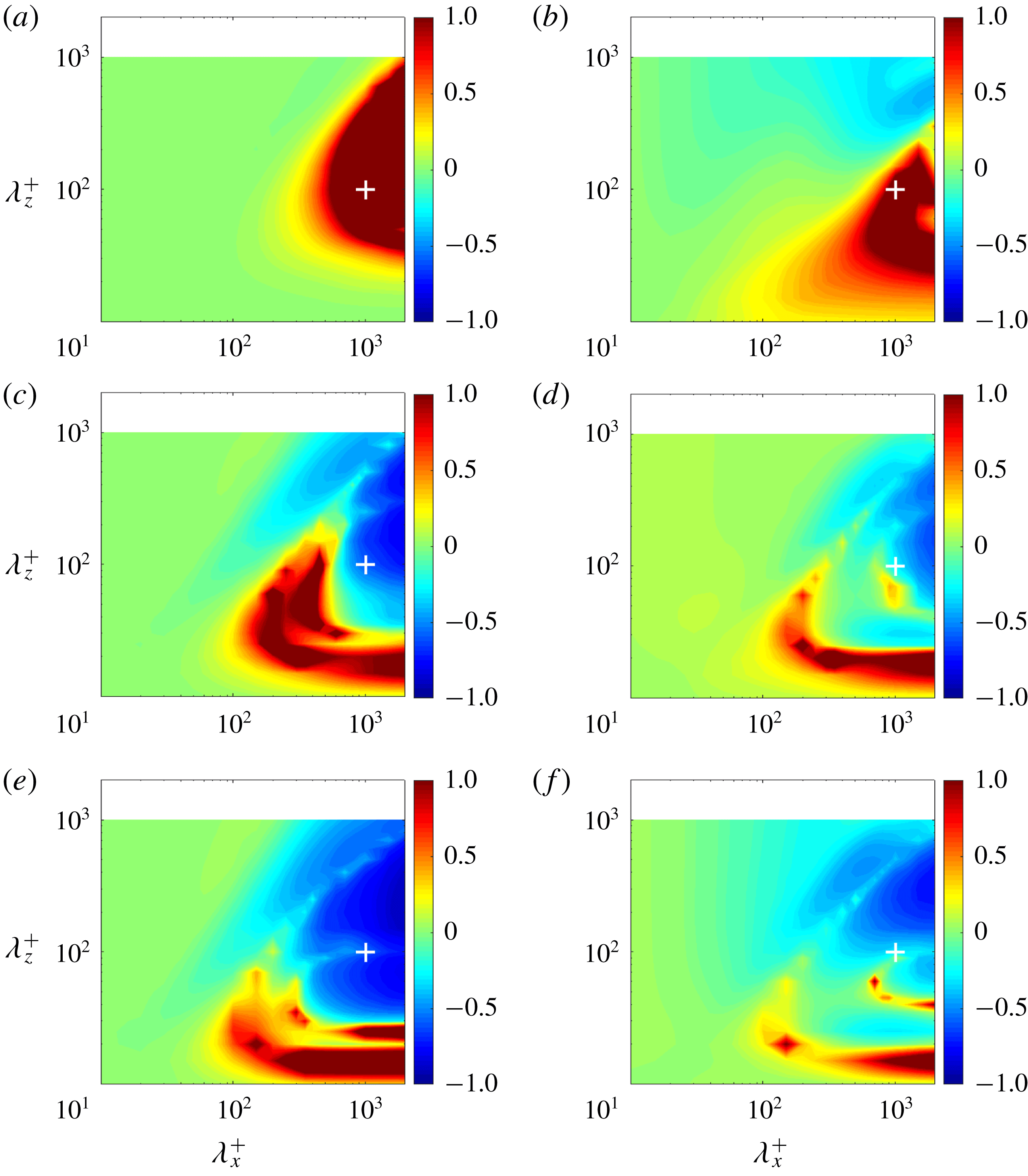
Acknowledgements
The authors are grateful to Dr Z. Xia (Peking University) for providing DNS data for turbulent channel flow with SR. S.N. and K.F. are grateful to Drs S. Obi and K. Ando (Keio University) for fruitful discussions. This work was supported through JSPS KAKENHI grant nos 25420129 and 18H03758 by the Japan Society for the Promotion of Science (JSPS).
Appendix
As a preliminary sensitivity analysis, this appendix compares resolvent-based predictions obtained using the mean velocity profile computed from the Reynolds and Tiederman eddy viscosity model (RT model) against resolvent-based predictions obtained using mean profiles from DNS of rotating channel flow at
 $Re_{\unicode[STIX]{x1D70F}}=180$
(Xia et al.
Reference Xia, Shi and Chen2016).
Relationship between
 $Ro_{\unicode[STIX]{x1D70F}}$
and
 $(\unicode[STIX]{x1D70E}_{\boldsymbol{k}c}/\unicode[STIX]{x1D70E}_{\boldsymbol{k}0})$
. Black circles show predictions obtained using the RT model for both non-rotating and rotating cases. Red crosses show predictions obtained using the RT model for the non-rotating case and DNS data for rotating cases.

Figure 11 shows the normalized change in singular values for rotating channel flow relative to the non-rotating case at
 $Re_{\unicode[STIX]{x1D70F}}=180$
:
 $(\unicode[STIX]{x1D70E}_{\boldsymbol{k}c}/\unicode[STIX]{x1D70E}_{\boldsymbol{k}0})-1$
. Figure 11(a,c,e) shows results obtained using the RT model for both rotating and non-rotating cases, while figure 11(b,d,f) shows results obtained using the RT model for the non-rotating case and DNS profiles for rotating cases. At each rotation number, the overall trend is similar in both scenarios, though there are important qualitative differences. As an example, at
 $Ro_{\unicode[STIX]{x1D70F}}=1$
, the amplified region (red) in figure 11(a) for
 $\unicode[STIX]{x1D706}_{z}^{+}\gtrapprox 300$
is replaced by a region of suppression (blue) in figure 11(b).
For a more quantitative evaluation of these differences, we focus on modes resembling the NW cycle, i.e. the modes with
 $(\unicode[STIX]{x1D706}_{x}^{+},\unicode[STIX]{x1D706}_{z}^{+},c^{+})\approx (10^{3},10^{2},10)$
considered in § 3.1. Figure 12 shows the effect of the rotation rate,
 $Ro_{\unicode[STIX]{x1D70F}}$
, on the singular value ratio,
 $(\unicode[STIX]{x1D70E}_{\boldsymbol{k}c}/\unicode[STIX]{x1D70E}_{\boldsymbol{k}0})$
. The black circles in figure 12 are the same as those in figure 7(a), while the red crosses show predictions obtained using mean profiles from DNS. For the DNS profile-based predictions (red crosses), the singular value ratio initially increases monotonically with increasing rotation number; maximum amplification is observed at
 $Ro_{\unicode[STIX]{x1D70F}}=1$
. For
 $Ro_{\unicode[STIX]{x1D70F}}\geqslant 2.5$
, the singular value ratio decreases monotonically, indicating that the NW modes are suppressed relative to the non-rotating case. These trends are again qualitatively consistent with the RT model-based predictions (black circles). However, there are some important differences: at
 $Ro_{\unicode[STIX]{x1D70F}}\approx 2.5$
, the black circles show very high amplification, while the red crosses indicate suppression. Interestingly, the model-based predictions show better agreement with the DNS results of Yang & Wu (Reference Yang and Wu2012) discussed in § 3.1.
Nevertheless, the results presented in this appendix suggest that resolvent analysis does not show extreme sensitivity to the mean profile when it comes to qualitative trends (e.g. the effect of rotation rates). However, there are local differences in mode amplification or suppression across spectral space.



