INTRODUCTION
Coastal barriers are sensitive to environmental dynamics. Micro- and mesotidal settings, gently dipping continental shelves, and sediment availability favor the development of coastal barriers (McCubbin, Reference McCubbin, Scholle and Spearing1982). Therefore, these environments have an increased possibility to record coastal evolution and environmental variations such as climate events and relative sea-level changes (Reading and Collinson, Reference Reading, Collinson and Reading1996; Van Heteren et al., Reference van Heteren, Huntley, van de Plassche and Lubberts2000; Plint, Reference Plint, James and Dalrymple2010; Tamura, Reference Tamura2012; Lima et al., Reference Lima, Dillenburg, Medeanic, Barboza, Rosa, Tomazelli, Dehnhardt and Caron2013; Dillenburg et al., Reference Dillenburg, Barboza, Rosa, Caron and Sawakuchi2017) as noted in studies discussing costal barrier formation and evolution (Tanner, Reference Tanner1995; Taylor and Stone, Reference Taylor and Stone1996; Otvos, Reference Otvos2000). Coastal barriers can also preserve records of ancient beach morphodynamic stages (e.g., Short and Hesp, Reference Short and Hesp1982; Taylor and Stone, Reference Taylor and Stone1996).
The knowledge of these factors — coastal evolution and environmental variations — is very important in the understanding of climate change and depositional processes (e.g., Ainsworth et al., 2011; Johnson et al., Reference Johnson, Moore, Ells, Murray, Adams, MacKenzie and Jaeger2014; Cooper et al., Reference Cooper, Green and Loureiro2018; Moore and Murray, Reference Moore and Murray2018). Therefore, we explore paleomorphodynamic aspects (number of breaker bars, beach gradient variations), recurrence time of severe storms, progradation rates, and relative sea-level changes along the entire Holocene micro-tidal barrier located on the coastal plain of Rio Grande do Sul State, southernmost Brazil. This coastal plain contains the most complete Quaternary record along the Brazilian coastline (Tomazelli and Villwock, Reference Tomazelli and Villwock1992), and includes a Holocene barrier formed during the last 7 ka (Dillenburg et al., Reference Dillenburg, Roy, Cowell and Tomazelli2000).
Studies discussing the formation and evolution of coastal barriers using ground-penetrating radar (GPR) and optically stimulated luminescence dating (OSL) are common due to the excellent results obtained by these methods (e.g., Tamura et al., Reference Tamura, Murakami, Nanayama, Watanabe and Saito2008; Tamura, Reference Tamura2012; Billy et al., Reference Billy, Robin, Hein, Certain and FitzGerald2015; Oliver et al., Reference Oliver, Thom and Woodroffe2016; Dillenburg et al., Reference Dillenburg, Barboza, Rosa, Caron and Sawakuchi2017). Thus, we acquired and used data from both GPR and OSL and compared the results with modern beach profiles.
Our description of an extensive sand barrier relies on a qualitative analysis of the sigmoidal-shaped, seaward-dipping reflectors and associated hummocky features, and on the quantitative comparison between the GPR data and the gradient, extent, maximum depth, number, and spacing of breaker bars from the present beach. These comparisons with the modern shoreline made it possible to elaborate on a beach profile model, which led us to an interpretation of reflectors that differs relative to some previous models (Dillenburg et al., Reference Dillenburg, Tomazelli and Barboza2004, 2017; Dillenburg and Barboza, Reference Dillenburg and Barboza2014; Hede et al., Reference Hede, Sander, Clemmensen, Pejrup and Nielsen2015; Rosa et al., Reference Rosa, Barboza, Abreu, Tomazelli and Dillenburg2017) and is in agreement with other previous models (e.g., Rodriguez and Meyer, Reference Rodriguez and Meyer2006; Bristow and Pucillo, Reference Bristow and Pucillo2006; Rodriguez et al., 2008). The reflectors that are continuous and gently dipping towards the ocean are related to the backshore/foreshore and upper shoreface environments. The underlying irregular, discontinuous, flat-to-sinuous reflectors are related to the lower shoreface. This compartmentation differs from previous works (Dillenburg et al., Reference Dillenburg, Tomazelli and Barboza2004, Reference Dillenburg, Barboza, Rosa, Caron and Sawakuchi2017; Dillenburg and Barboza, Reference Dillenburg and Barboza2014; Hede et al., Reference Hede, Sander, Clemmensen, Pejrup and Nielsen2015; Rosa et al., Reference Rosa, Barboza, Abreu, Tomazelli and Dillenburg2017) where the parallel/inclined reflectors are related to the foreshore and the irregular underlying reflectors are related to the upper shoreface. Our methodology allowed us to obtain important information for improving our knowledge of coastal evolution, and to infer climate changes in the study area. Thus, our approach brings new information understanding of evolution of this coastal barrier and to the ancient morphodynamic stages of sand barriers.
Regional setting
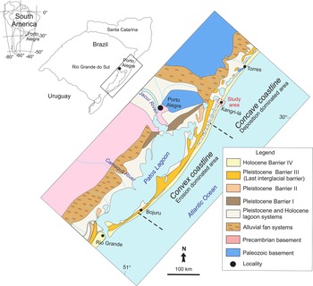
The coastal plain of Rio Grande do Sul State, located in the southernmost portion of the Brazilian continental margin, represents the emerged part of the Pelotas Basin, which is related to the opening of the Atlantic Ocean (Asmus and Porto, Reference Asmus and Porto1972). The coastal plain contains alluvial fans as well as three Pleistocene and one Holocene juxtaposed lagoon-barrier systems created by successive transgressive-regressive (TR) cycles (Fig. 1; Villwock, Reference Villwock1984; Tomazelli and Villwock, Reference Tomazelli, Villwock, Holz and De Ros2000; Dillenburg et al., Reference Dillenburg, Barboza, Tomazelli, Hesp, Clerot, Ayup-Zouain, Dillenburg and Hesp2009). The last TR cycle is responsible for the formation of the Holocene barrier that is the subject of this study. According to Angulo et al. (Reference Angulo, Lessa and de Souza2006), the Holocene barrier and adjacent lagoons registered the last marine transgression that ended between 7.7 ka and 6.9 ka. Relative sea level reached its maximum height of ~3 m above the modern level ca. 6 ka, then dropped to its modern position.
Maps indicating the location of the study area within South America, southern Brazil, and on a geological map of the Coastal Plain of Rio Grande do Sul State (modified after Dillenburg and Barboza, Reference Dillenburg and Barboza2014).

The gently sloping inner continental shelf (0.027° to 0.125°; Dillenburg et al., Reference Dillenburg, Roy, Cowell and Tomazelli2000) is bordered by dissipative to intermediate beaches (Toldo et al., Reference Toldo, Almeida, Dillenburg, Tabajara, Ferreira and Borghetti1993; Calliari et al., Reference Calliari, Klein and Barros1996). The coastal sands in this area are fine- to very fine-grained and consist of ~97% quartz grains (Carassai et al., Reference Carassai, Lavina, Chemale and Girelli2018). Bioclast concentrations were observed in a few sites where marine erosion dominates (Calliari et al., Reference Calliari, Klein and Barros1996).
Along the coastal barrier, the tide is semi-diurnal and has a mean range of 0.5 m (Dillenburg et al., Reference Dillenburg, Barboza, Tomazelli, Hesp, Clerot, Ayup-Zouain, Dillenburg and Hesp2009). Two high-pressure centers control wave regime: the South Atlantic Anticyclone and the Polar Mobile Anticyclone. The South Atlantic Anticyclone dominates during spring and summer, generating northeasterly winds. The Polar Mobile Anticyclone dominates during the fall and winter, and creates southwesterly winds (Tomazelli, Reference Tomazelli1993). Storms deriving from the action of the Polar Mobile Anticyclone can raise sea level (meteorological tides) up to 1.9 m for short periods (Parise et al., Reference Parise, Calliari and Krusche2009). Net littoral drift moves sand in a northeasterly direction (Tomazelli and Villwock, Reference Tomazelli and Villwock1992; Toldo et al., Reference Toldo, Almeida, Dillenburg, Tabajara, Ferreira and Borghetti1993).
The Holocene sand barrier is >700 km long, is present in in Brazil and Uruguay, and encompasses the entire Rio Grande do Sul State coastline (~500 km long). However, its width is quite variable, ranging from 18 km at Cassino Beach, thinning out to areas where its width is zero, and the Holocene barrier has been entirely removed by marine erosion (e.g., Hermenegildo Beach). This remarkable difference results from zones where either erosion (convex coastline) or deposition (concave coastline) dominate along the coastline (Fig. 1). Dillenburg et al. (Reference Dillenburg, Roy, Cowell and Tomazelli2000), Lima (Reference Lima2012), and Dillenburg and Barboza (Reference Dillenburg and Barboza2014) assigned this differentiation to oceanographic processes; more specifically, to differentiation of wave energy dissipation and longshore currents along the coastline. However, we relate this zonation to differential isostatic movements that led to the creation of relative uplift (erosion) and subsidence (deposition) zones along the coast. Therefore, distinct oceanographic processes along the coastal barrier are driven by coastal morphology rather than its cause.
This study focuses on the northern portion of the Holocene barrier in Xangri-lá County (Fig. 1), where the barrier is ~3 km wide. The shoreface displays a moderate slope (varying between a gradient of 0.011 to 0.021, or 0.009° to 0.019°) and is composed of well-sorted, very fine- to fine-grained sand (Gruber et al., Reference Gruber, Toldo, Barboza and Nicolodi2003, Reference Gruber, Toldo, Barboza, Nicolodi and Ayup-Zouain2006b). During fall and winter, the beach displays a dominant dissipative profile due to frequent storms, whereas during spring and summer, it shows an intermediate profile (Machado et al., Reference Machado, Calliari, Melo and Klein2010). Its surf zone usually contains three bars. During beach accretion, coupling of the intermediary and inner bars may occur. Larger, moderate, and smaller waves dissipate their energy on the outer, intermediary, and inner bars, respectively, which are ~300 m, ~160 m, and ~90 m oceanward from the foreshore (Tabajara et al., Reference Tabajara, Almeida and Martins2008).
METHODS
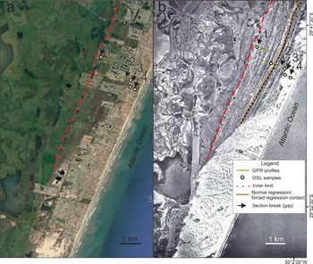
The study relies on geological and geomorphological data obtained from Google Earth (https://earth.google.com/web) images, GPR surveys, and OSL dating. In addition, we used aerial photographs from the Geological Survey of Brazil (CPRM) taken in 1964 before intense urbanization took place from the 1970s to present that caused the removal of most of the eolian dunes (Fig. 2).
Images showing locations where GPR profiles and OSL samples were taken: (a) base photo from Google Earth (https://earth.google.com; accessed March 2020), (b) aerial photo from 1964 provided by the Geological Survey of Brazil. Note intense urbanization in the Google Earth image. The contact between normal regression and forced regression and the landward (inner) limit of the Holocene barrier are also shown.

Ground-penetrating radar (GPR)
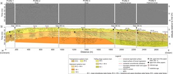
GPR acquisition was performed along flat, almost-horizontal roads and smoothed terrains. Subsurface data come from five complementary GPR profiles acquired perpendicular to the shoreline (Figs. 2, 3). Together, the profiles display 2.78 km of subsurface data that cover the entire width of the Holocene barrier (Fig. 2). GPR acquisition was performed using a RAMAC MALA® Georadar operating with a 250 MHz shielded antenna. Data processing was done in Reflexw® software v. 4.5 (https://www.sandmeier-geo.de/reflexw.html) and included the following steps: set time zero, filters and gain, velocity analysis (determination of wave velocity by hyperbole superposition method), migration, and topographic correction. The hyperbole adjustment method was applied for subsurface velocity evaluation and time-to-depth conversion, resulting in a velocity of 0.06 m/ns. This is the expected velocity for water-saturated sands (Neal and Roberts, Reference Neal and Roberts2000), and it is a logical result considering that the water table in the region is very shallow, being only a few tens of centimeters deep in the area. The vertical resolution of GPR data is ~25 cm.
Data interpretation was an adaptation of the seismic stratigraphic method (Payton, Reference Payton1977) to GPR profiles (Neal, Reference Neal2004). Hence, reflector geometry, patterns, and terminations (onlap, downlap, toplap) were analyzed. For topographic correction, altitude was measured in each measurement using a total station and the Leica TS15 optical prism. Topography was adjusted to modern mean sea level (msl) using the RN 178IF reference level of the Instituto Brasileiro de Geografia e Estatística (IBGE).
Current beach morphology was also investigated to compare and associate recent features with subsurface features recorded in the GPR profiles. We used a modern beach profile created by Tabajara et al. (Reference Tabajara, Almeida and Martins2008) and Google Earth (https://earth.google.com; accessed May 2018) images for our modern beach morphology profile. Based on this dataset, we measured several parameters (distance from the beginning of the sigmoidal depositional units and length, depth, and dip of the main morphological elements) to compare modern and ancient beach features.
Optically stimulated luminescence (OSL) ages
Approximately 2.54-cm-wide and ~10.16-cm-long aluminum tubes were used for sampling and storage of material for OSL dating (Figs. 2, 3). Trenches were dug to sample the material and to observe the water table level. Sampling was performed with a tube in a horizontal, strike-oriented position in order to sample sediments of the same layer. Collected material was sent to the Dating and Dosimetry Laboratory of the Universidade Federal de São Paulo (UNIFESP). OSL samples were cleaned with H2O2 for two hours to remove organic material, and then washed with distilled H2O, immersed in 30% hydrofluoric acid (HF) for 45 minutes to remove carbonates and the surface of the quartz grains, thus eliminating ionization from the α-particle, then washed again with distilled H2O. The samples were then immersed in 10% HCl for two hours to eliminate possible fluorides formed during the HF bath, then washed again with distilled water. Finally, samples were immersed in sodium polytungstate (SPT) to eliminate feldspar (density = <2.62 g/cm3) and heavy minerals (density = >2.75 g/cm3) to obtain pure quartz grains.
(a) GPR profiles of barrier in the Xangri-lá County and (b) interpretation of radar facies. Note the three distinct systems tracts: transgressive, highstand, and falling stage. Black dashed line represents the limit between the normal regression (NR) and forced regression (FR). Ages from this study given in Table 1; ages from other studies and references given in Table 2; ns is nanoseconds.

Natural radioactive contents (U, Th, and 40K) were determined by γ-spectroscopy, and the spectra of the samples from sediments close to the edges of the tubes were measured with a Canberra Inc. hyper-pure germanium (HPGe) detector with ultra-low background shield and compared to the soil-pattern spectra for JR-1, 182 JB-3, JG1a, and JG-3 using the GSJ standards of the geochemical reference samples database. Contributions of cosmic radiation were calculated using equations from Prescott and Hutton (Reference Prescott and Hutton1994). Finally, the annual dose rates were calculated based on the U, Th, and 40K concentrations using the conversion factors of Guérin et al. (Reference Guérin, Mercier and Adamiec2011). Radiation and luminescence readings were performed in a Risø OSL/TL DA-20 and DA-15 with blue-light stimulation, Hoya U-340 filters, and a 90Sr/90Y integrated beta source. The radial plot was used to analyze the distribution of equivalent doses (Galbraith and Roberts, Reference Galbraith and Roberts2012), overdispersion (OD) values were evaluated, and the central age model (CAM; Galbraith et al., Reference Galbraith, Roberts, Laslett, Yoshida and Olley1999) was applied to calculate the final De (equivalent dose). The two samples from the oldest portion of the Holocene barrier (B4-9M and B4-0M; Table 1) came from the lower part of the eolian deposits, ~ 2 m below the surface. Younger samples collected closer to the ocean were taken ~40 cm below the surface, also from eolian deposits. At these sites, a high water table precluded sampling from deeper levels.
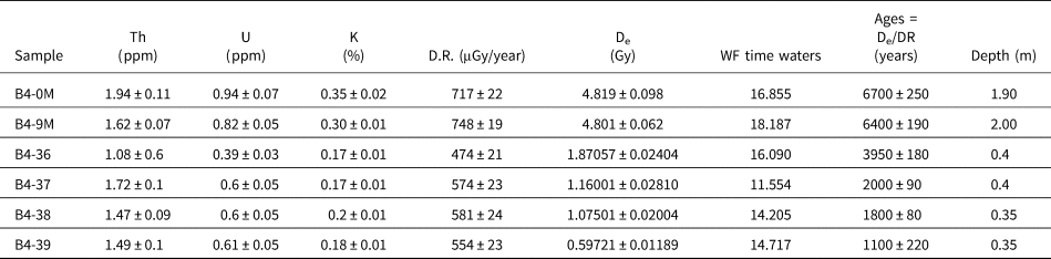
Results for samples dated by the OSL method, including radionuclide concentrations (238U, 232Th, and K), dose rate (DR), equivalent dose (De) data used for calculation of OSL ages. W is the saturation water content and F is the fraction of saturation corresponding to the assumed average water content over the entire burial period.

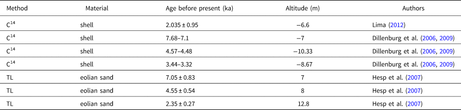
In addition to the ages presented here, the evolution of the Holocene barrier was also supported by previously dated sites nearby (Dillenburg et al., Reference Dillenburg, Tomazelli, Hesp, Barboza, Clero and da Silva2006, Reference Dillenburg, Barboza, Tomazelli, Hesp, Clerot, Ayup-Zouain, Dillenburg and Hesp2009; Hesp et al., Reference Hesp, Dillenburg, Barboza, Clerot, Tomazelli and Ayup-Zouain2007; Lima, Reference Lima2012). These previous results (Table 2) were projected into our section following the almost parallel-to-coastline vegetated eolian dunes, within the same facies, and at the same position relative to mean sea level. Next, these ages were transposed onto the most proximal point of the associated ridge, just below the limit between eolian and beach deposits. This procedure was performed to compare the eolian (this study) and beach (Table 2) sediment ages. It is worth noting that the ages of the beach sands and the eolian deposits resting on top of them are a quite good match.
Previously published ages for the northern portion of the PCRS. The ages presented by Dillenburg et al. (Reference Dillenburg, Tomazelli, Hesp, Barboza, Clero and da Silva2006) were calibrated and later published in Dillenburg et al. (Reference Dillenburg, Barboza, Tomazelli, Hesp, Clerot, Ayup-Zouain, Dillenburg and Hesp2009).

Relative sea-level envelope
The limit between the eolian and beach deposits along a certain time is a proxy for the changes of the relative sea level during this same time interval. We plotted the available chronological data (Table 1, Table 2) and the respective altimetric positions relative to current msl of the boundary between the eolian and beach deposits taken from our GPR data. The connection of the altimetric values of this limit along time delineates the upper limit of a relative sea-level envelope if no erosion has taken place (i.e., it records the trajectory of the foredune base). However, this surface may include minor or major erosion, down to the actual relative sea level 1.5 m below the foredune base in the same region (Barboza et al., Reference Barboza, Dillenburg, Ritter, Angulo, da Silva, da Camera Rosa, Caron and de Souza2021). Considering these data, we constructed a curve 1.5 m below the upper limit of the relative sea-level envelope to delineate the lower boundary of the relative sea-level envelope. Therefore, this envelope includes all possible positions of relative sea level along an analyzed time interval.
RESULTS
Description
In the studied area, the Holocene coastal barrier is 2.78 km wide. A 1964 aerial photograph (Fig. 2b) displays a series of roughly parallel, slightly sinuous, inactive, low-relief dunes nearly parallel to the present coastline that we interpret as poorly developed transgressive dune fields attached to the foredune. There are a similar number of eolian ridges (Fig. 2b) and sigmoidal erosive surfaces in the beach facies (Fig. 3), suggesting a relationship between beach erosion and eolian accumulation. Eastwards and southwards, truly transgressive, mostly active dune fields occur. Since 1964, urban growth has expanded to occupy the transgressive dune field, including where GPR lines were acquired close to the present coastline (Fig. 2). The uneven distance between the ridges due to their slightly sinuous shape resembles the external limits of currently active dune fields. In accordance with Hesp et al.'s (Reference Hesp, Dillenburg, Barboza, Tomazelli, Ayup-Zouain, Esteves, Gruber, Toldo, Tabajara and Clerot2005) criteria, these features were therefore interpreted as the landward border of poorly developed transgressive dune fields instead of beach ridges.
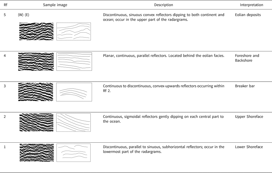
The GPR section presents good resolution up to 10 m deep (Fig. 3). Close to the modern beach, signal quality abruptly declines due to the presence of a saline wedge. Five radar facies (Rf) were identified (Table 3). Rf 1 occurs in the lowermost portion of the radargrams and comprises a > 2-m thick package defined by discontinuous, irregular, sinuous, subparallel to parallel reflectors that dip both onshore and offshore (Figs. 3, 4). Rf 2 encompasses a 3- to 5-m-thick interval composed of continuous, sigmoidal reflectors that dip gently seaward (mean dip = 1.7°), and merge downslope and upslope into Rf 1 and Rf 4, respectively (Figs. 3, 4). Closely associated with Rf 2, there are two to three 20 to 50 m long and up to 1 m high sets of continuous to discontinuous, convex-upward reflectors (hummocky geometry) that constitute Rf 3 (Figs. 3, 4). Rf 4 is composed of continuous, parallel, and subhorizontal reflectors that grade seawards to the steeper reflectors of Rf 2 (Figs. 3, 4). Rf 5 comprises the uppermost interval that gradually thins towards the ocean (Fig. 3). This package is 0.5 to 4 m thick and rests on an erosive to bypass surface (diastem) above Rf 4 (Fig. 5). It is composed of (1) sub-horizontal, discontinuous, irregular, sinuous, subparallel to parallel reflectors, (2) wide sets (> 50-m wide and > 1-m thick) of trough cross-bedded reflectors, and (3) asymmetrical or symmetrical (mound or hummocky geometry) reflectors dipping towards both the ocean and continent.
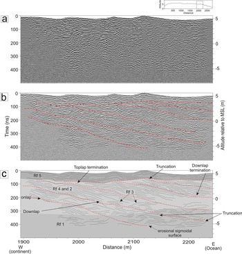
Bounding surfaces analyses (see small upper figure for the location of the radargram within the entire GPR section given in Figure 3): (a) uninterpreted radargram; (b) partially interpreted radargram delineating the largest boundaries (red dashed lines), including contacts among sigmoidal sand units as well as between them and the overlying eolian unit; and (c) entirely interpreted radargram showing the relationships between internal reflectors and bounding surfaces (truncation, downlap, toplap, and onlap).

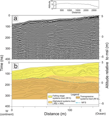
(a) Radargram and (b) interpretation of part of the overall GPR section shown in Figure 3 (see small upper figure in (a) for location of radargram within the entire GPR section), showing the limit between transgressive and highstand systems tracts. The surface between these facies is interpreted as a maximum flooding surface (MFS).

Radar facies (Rf) description and interpretation based on reflection configuration.

The Rf 5/Rf 4 boundary constitutes the most extensive stratigraphic surface in the GPR cross section (Fig. 3). Its position above present sea level varies from 1 m at the western limit of the cross section, then it rises to up to 4 m along the intermediate portion of the section, and gradually falls to 1.3 m above present sea level near the modern shoreline (Fig. 3). Below this major surface, the entire package contains 28 increments of sigmoidal sandy units that gently dip towards the ocean (Fig. 3). The sigmoidal bounding surfaces truncate earlier reflectors (erosional phase) and are overlain during the ensuing depositional phases (Figs. 4, 6). The sigmoidal sand units are initially gentler (0.5° to 0.8°) and become steeper (0.9° to 1.6°) from 1,900 m to the end of the cross section (Fig. 3).
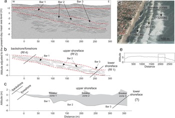
Comparison between (a) GPR data and (b) interpretation of this study, (c) modern beach profile from Tabajara et al. (Reference Tabajara, Almeida and Martins2008), and (d) satellite image from Google Earth (https://earth.google.com; accessed May 2018); GPR line location is presented in (e). To facilitate the comparison between the ancient (a, b) and modern (c, d) beach profiles, altitude and distance as shown in (e) were adjusted based on the present position of the foreshore/shoreface transition. Note that the actual horizontal spacing of subenvironments (breaker bars, foreshore/backshore, upper and lower shoreface) is similar to the ancient beach profile (GPR data).

Table 1 presents luminescence dating data. Accepted aliquots showed recycling rates from 0.9 to 1.1 and recuperation values smaller than 5%. Equivalent dose distribution shows 3% to 12% over dispersion values. Because equivalent dose dispersion is small, a CAM allows for the determination of equivalent dose values (Galbraith and Roberts, Reference Galbraith and Roberts2012). Dating along the section allowed us to estimate barrier age (ca. 7.1 ka), and to date the main associated phases related to relative sea-level trajectory (Fig. 3). It should be noted that only the upper eolian deposits (Rf 5) were dated by OSL.
The oldest dated sample in our section (6.7 ka) came from a location situated ~200 m from the section origin (Fig. 3, Table 1). Approximately 20 m from this first sampling site (sample B4-0M; Table 1), another sample (B4-9M; Table 1) was collected and analyzed. The ages of both samples are similar (6.70 ± 0.25 ka and 6.40 ± 0.19 ka). A sample collected 1,440 m seaward from the inner limit of the barrier where the Rf 4/Rf 5 boundary reaches its highest position (Fig. 3), ~4 m above msl, was dated at 3.95 ka. The path of the Rf 4/Rf 5 boundary around its highest position is smooth. Samples dated as 2 ka and 1.8 ka are located 2,100 m and 2,300 m seaward from the inner limit of the barrier, respectively, where the Rf 4/Rf 5 limit altitude is ~3.3 m above msl. The 1.1 ka age at 2,500 m seaward from the inner limit of the barrier is ~2.5 m above msl (Fig. 3).
Interpretation
GPR section and beach profile
The radar facies description provides the basic evidence to create a beach profile model (Fig. 6). The stratal relationship indicates two distinct beach profiles: one erosive and gently dipping, and another depositional and steeper. Therefore, the gently dipping erosional sigmoidal surfaces (Figs. 3, 4, 6) limit sets of slightly steeper reflectors that delineate progradational pulses of the barrier (Figs. 3, 5). The erosive boundaries record discontinuities associated with increased wave energy, sediment input change, or rapid sea-level fluctuations (Johnston et al., Reference Johnston, Thompson, Baedke, Baker and Jol2007). During storm surges, the beach is flooded and partially eroded (Parise et al., Reference Parise, Calliari and Krusche2009; Machado et al., Reference Machado, Calliari, Melo and Klein2010; Guimarães et al., Reference Guimarães, Farina, Toldo, Diaz-Hernandez and Akhmatskaya2015). We related these sigmoidal surfaces, or diastems, to erosional events produced by severe storms. These 28 sigmoidal depositional sets (Fig. 3) show similar thicknesses along the section (2.9, 2.3, and 2.5 m for the maximum, minimum, and mean thickness), suggesting a periodic or quasiperiodic organization. Based on an estimated age of 7.1 ka for the entire barrier, and the presence of 28 sigmoidal depositional sets, each depositional increment is inferred to record ca. 250 years of sedimentation/beach progradation. We analyzed radar facies changes along the dips of the sigmoidal depositional sets (Fig. 6), and used the eolian/beach bounding surface as the inner limit for the description of the downdip facies tracts.
Rf 1 appears from 5 to 7 m below the eolian/beach boundary (Figs. 3, 6). Following a single depositional surface, these uppermost deposits (i.e., the shallower portion of this facies) record sedimentation taking place ~300 m seaward from the eolian/beach boundary. The undulating, discontinuous, and subhorizontal nature of Rf 1 is compatible with a depositional setting dominated by oscillatory flows (Fig. 6b). All together, these pieces of evidence match what should be expected for a lower shoreface setting.
Rf 2 and Rf 4 occur from the eolian/beach limit to depths of 5–7 m. Their dip extent ranges from 250 to 300 m along a slope with a mean declivity of 0.02 or 1.3°. According to Gruber et al. (Reference Gruber, Corrêa, Nicolodi and Barboza2006a), the modern, high-energy beach zone (foreshore and upper shoreface) in this part of the coastal plain extended downwards to 6 m depth and presented a gradient of about 0.021. Tabajara et al. (Reference Tabajara, Almeida and Martins2008) indicated that the modern upper shoreface is 300-m long. Therefore, the depth of the boundary between the lower and upper shoreface, the beach zone horizontal distance, and its gradient are remarkably like those recorded in the GPR section. The striking similarity between both modern and ancient beach profiles supports the inference that Rf 2 corresponds to the upper shoreface.
Rf 2 includes two to three sets of sigmoidal bodies (Rf 3) positioned approximately 90, 150/200 and 250/300 m seaward from the shoreline within each distinct depositional unit (Fig. 6b). The Rf 3 reflectors’ geometry and spacing match the shape and position of the three modern breaker bars (compare Fig. 6b, c, and d). The second bar may be more complex, and composed of two partially amalgamated bars (Fig. 6b, c).
However, some authors have related the inclined, seaward-dipping reflectors (Rf 2) and the underlying sub-horizontal, parallel to sinuous (Rf 1) reflectors to backshore/foreshore and upper shoreface settings, respectively (Dillenburg et al., Reference Dillenburg, Tomazelli and Barboza2004, Reference Dillenburg, Barboza, Rosa, Caron and Sawakuchi2017; Dillenburg and Barboza, Reference Dillenburg and Barboza2014; Hede et al., Reference Hede, Sander, Clemmensen, Pejrup and Nielsen2015; Rosa et al., Reference Rosa, Barboza, Abreu, Tomazelli and Dillenburg2017). We disagree based on a quantitative comparison between our radargrams (shape, declivity, continuity, and depths of the reflectors) and a beach profile of the same region by Tabajara et al. (Reference Tabajara, Almeida and Martins2008).
The near-horizontal reflectors at the landward end of the sigmoidal sand units were interpreted as foreshore/backshore facies (Rf 4). Within each depositional sigmoidal increment, this facies is up to 0.5 m thick and 50 m to 90 m long. These figures are also compatible with the modern backshore/foreshore extent. Additionally, the distance between inner bar and shoreline and the geometry of this segment of the beach profile also match the size and geometry of the horizontal reflectors that characterize the landward edge of the sigmoidal bodies (Fig. 6b, c). Therefore, we related these horizontal reflectors to the foreshore and backshore facies (Rf 4) that could have been partially eroded as shown by the truncated reflectors shown in Figure 4. This interpretation agrees with other authors who also described radar facies interpreted as foreshore and upper shoreface deposits together (e.g., Tercier et al., Reference Tercier, Knight and Jol2000; Bristow and Pucillo, Reference Bristow and Pucillo2006; Rodriguez and Meyer, Reference Rodriguez and Meyer2006).
Finally, the uppermost radar facies (Rf 5) corresponds to the exposed eolian deposits formed by southwestward-migrating parabolic (hummocky reflectors) and barchan (wide sets of trough cross-bedded reflectors) dunes and associated interdunes (sub-horizontal, irregular, subparallel to parallel reflectors) (Fig. 3). At the base of the innermost portion of the section (first 150 m), large-scale sets of cross-bedded reflectors ~1.5-m thick and >50 m wide were associated with Holocene eolian barchan dunes (7.1 ka, Dillenburg et al., Reference Dillenburg, Tomazelli, Hesp, Barboza, Clero and da Silva2006). Foreshore and upper shoreface deposits of Rf 2 and Rf 4 overlie these eolian deposits (Fig. 5).
Relative sea-level and progradation rates
Radar facies interpretation (Table 3) and OSL ages (Table 1), associated with ages published elsewhere (Table 2), made it possible to describe the evolution of the Holocene barrier (Fig. 3). It is important to note that the luminescence data indicate well-bleached sediments and no post-depositional mixing. As pointed out by other authors, the Holocene barrier contains a sedimentological record of the last 7 ka (e.g., Dillenburg et al., Reference Dillenburg, Tomazelli, Hesp, Barboza, Clero and da Silva2006, Reference Dillenburg, Barboza, Rosa, Caron and Sawakuchi2017; Hesp et al., Reference Hesp, Dillenburg, Barboza, Clerot, Tomazelli and Ayup-Zouain2007; Lima, Reference Lima2012).
Stratigraphic analysis of the GPR data shows three distinct depositional elements associated with the transgressive (TST), highstand (HST), and falling stage (FSST) systems tracts (Hunt and Tucker, Reference Hunt and Tucker1992). The TST occurs only in the first 150 m of the GPR cross section, where eolian deposits (Rf 5) are overlain by foreshore and upper shoreface facies (Rf 2 and Rf 4). In this first 150 m, the boundary between the eolian and beach deposits is interpreted as the maximum flooding surface, which delineates the beginning of a HST (Figs. 3, 5). The 6.7 ka age of the eolian (Rf 5) facies suggests that the TST is older. According to Dillenburg et al. (Reference Dillenburg, Tomazelli, Hesp, Barboza, Clero and da Silva2006, Reference Dillenburg, Barboza, Tomazelli, Hesp, Clerot, Ayup-Zouain, Dillenburg and Hesp2009), the Holocene coastal barrier in the Curumim area, ~20 km north of the study area, was already prograding ca. 7.1 ka. By projecting this age into our section, we estimate that the HST begun ca. 7.1 ka. Based on micropaleontological, stratigraphic, and chronological data from a nearby location, Lima (Reference Lima2012) dated the end of the TST at 7.2 ka. Therefore, we assume that the end of the transgression and onset of coastal barrier progradation took place at 7.1 ka (Fig. 3).
In terms of the ensuing regressive phase, it is important to note that the sector comprising the backshore/shoreface and/or the innermost portion of the upper shoreface is entirely preserved as sigmoidal sand units (Fig. 3). Therefore, the altitude of the limit between the eolian/innermost portion of the sigmoidal sand units approximates the position of relative sea level. Sea-level rise and fall may also be followed by another boundary that delineates the contact between the upper and lower shoreface (Fig. 3). Because both boundaries are parallel to each other and following the same trend along the entire section, the variation in the eolian/beach facies boundary can be used as an indicator of relative sea-level changes. Therefore, the regressive phase of the Holocene barrier comprises two systems tracts (Fig. 2): a first systems tract associated with a stage of relative sea-level rise to stillstand (HST), and a second systems tract related to a period of relative sea-level fall (FSST). The HST (Fig. 3) is composed of two stages. The earlier stage records a slightly rising relative sea-level phase (0 m to 480 m), which lasted 1.5 ka (7.1 to 5.6 ka), and the second stage registers a stillstand (480 to 1440 m), which persisted for 1.7 ka (5.6 to 3.9 ka). Therefore, the progradational rate of the barrier during the HST changed from 0.32 m/year (aggradational phase) to 0.5 m/year (stillstand).
The FSST includes two progradational stages. The first stage covers a period of a slow rate of relative sea-level fall and was observed between 1,440 and 2,340 m (3.9 to ca. 1.8 ka). The second stage, in which the rate of relative sea-level fall accelerates, is represented by the segment between 2,340 and 2,780 m that covers a period of 1.8 ka. Thus, the progradational rates of the barrier varied from 0.5 m/year (lower rate of relative sea-level fall) to 0.3 m/year (higher rate of relative sea-level fall).
The progradational rates were calculated using the ages obtained in this study. We only used our ages in the calculation of the progradation rates to eliminate additional sources of error. Previously calculated ages from beach facies close to the study area (Dillenburg et al., Reference Dillenburg, Tomazelli, Hesp, Barboza, Clero and da Silva2006; Hesp et al., Reference Hesp, Dillenburg, Barboza, Clerot, Tomazelli and Ayup-Zouain2007; Lima et al., Reference Lima, Dillenburg, Medeanic, Barboza, Rosa, Tomazelli, Dehnhardt and Caron2013) were correlated to our section, and showed a very good agreement. The age agreements for the backshore/foreshore and eolian facies indicate a small diastem between the eolian and beach deposits.
The trajectory of the limit between the eolian and beach deposits is a proxy for changes in relative sea level. From the position of this limit and respective ages (Fig. 3), we calculated the relative sea-level envelope (Fig. 7).
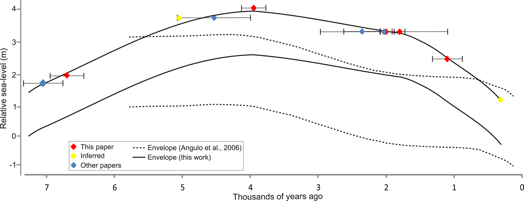
Holocene relative sea-level envelope for the studied area (solid line) based on ages and altimetric position of the contact between eolian and beach facies (Table 1 and Table 2; Fig 3). The horizontal error bar is related to confidence interval of age data. For comparison, the sea-level envelope curve of Santa Catarina State (dashed lines) is shown (Angulo et al., Reference Angulo, Lessa and de Souza2006).

During the aggradational phase of the HST, the relative sea level gradually rose at a rate of 1.8 mm/year, from 1.0 to 3.8 m above msl, and stayed constant from 5.6 to 3.9 ka. During the first phase of the FSST, relative sea level fell at a rate of 0.4 mm/year, from 3.8 m to 3.0 m. FInally, during the second phase, relative sea level fell at a rate of 1.6 mm/year, from 3 m to present msl.
DISCUSSION
Storms, beach profile, and morphodynamic inferences
The sigmoidal surfaces noted in our study are erosive, and record energy changes such as major storms (Figs. 3, 4). Erosive scours are only visible along the backshore/foreshore and upper shoreface deposits. Therefore, we think that deposition took place in the deeper setting of lower shoreface to offshore during these erosional events. Ancient storms have been studied through GPR profile in sand barriers, and sigmoidal surfaces are accepted as records of these events (e.g., Rodriguez and Meyer, Reference Rodriguez and Meyer2006; Tillmann and Wunderlich, Reference Tillmann and Wunderlich2013; Gontz et al., Reference Gontz, Moss and Wagenknecht2014; Goslin and Clemmensen, Reference Goslin and Clemmensen2017). The kind of severe storm recorded in our data could be like Hurricane Catarina, the first and the only hurricane recorded in the south of Brazil, so it is a rare event in the region. It occurred in March 2004 with winds of 44 m s-1 (85 kt) (McTaggart-Cowan and Bosart, Reference McTaggart-Cowan, Bosart, Davis, Atallah, Gyakum and Emanuel2006). Data suggests that severe storms are cyclical, but to confirm this cyclicity, a more detailed study of these sigmoidal surfaces by sediment cores and absolute ages is required (Dougherty et al., Reference Dougherty, FitzGerald and Buynevich2004; Clemmensen et al., Reference Clemmensen, Glad and Kroon2016; Goslin and Clemmensen, Reference Goslin and Clemmensen2017).
Beach morphology is mainly controlled by grain size, wave regime, and antecedent beach morphology (Sunamura and Horikawa, Reference Sunamura and Horikawa1974; Wright and Short, Reference Wright and Short1984; Wright et al., Reference Wright, Short and Green1985). In addition, the morphology and number of shoreface bars are directly related to the morphodynamic stage of the beach (Short and Aagaard, Reference Short and Aagaard1993; Gallagher et al., Reference Gallagher, Elgar and Guza1998). Because grain size does not vary in the studied area, changes in beach profile should reflect hydrodynamic fluctuations. Therefore, the seasonal nature of coastal winds and waves in southernmost Brazil is likely responsible for alternation between intermediate and dissipative beach morphodynamic stages (Tomazelli and Villwock, Reference Tomazelli and Villwock1992; Toldo et al., Reference Toldo, Almeida, Dillenburg, Tabajara, Ferreira and Borghetti1993). The intermediate morphodynamic beach stage is due to the action of fair weather waves that produce episodes of beach growth. This accretionary regime results in onshore shifts of the bars, and this bar migration can lead to the coupling of the internal and intermediate bars. Continuous accretion produces a gradually steeper beach profile and a smaller number of bars. The dissipative stage is the result of storm events in which high-energy waves erode the beach and transport sand to offshore. As a result, the beach profile becomes less steep. It is important to note that the external bar (bar farthest from the shoreline) is less mobile and, thus, has a greater potential for preservation (Lippmann and Holman, Reference Lippmann and Holman1990; Aagaard, Reference Aagaard1991; Lippmann et al., Reference Lippmann, Holman and Hathaway1993; Calliari et al., Reference Calliari, Muehe, Hoefel and Toldo2003).
Thus, the presence of two or three bars observed in the GPR section seems to indicate oscillations between dissipative and intermediate stages. Currently, this oscillation between dissipative and intermediate stages is annual and related to seasonal behavior associated with the regional wave regime (summer and winter). However, erosive events are much faster than accretion episodes (Machado et al., Reference Machado, Calliari, Melo and Klein2010; Machado and Calliari, Reference Machado and Calliari2016). Thus, it can be inferred that periods with numerous storm events tend to preserve a beach-ridge profile with three breaker bars. Periods in which fair weather conditions prevail tend to preserve two breaker bars. GPR data and the beach profile from Tabajara et al. (Reference Tabajara, Almeida and Martins2008) showed the intermediate breaker bar was segmented (Fig. 6).
Because the GPR section does not display a uniform quality, some areas had a very low resolution. Thus, it was not possible to quantify changes in the number of bars along the evolution of the coastal barrier during the Holocene, or to infer the most recurrent bar morphodynamic stage throughout the entire barrier. It is only possible to state that both dissipative and intermediate stages are recorded in the GPR section.
Analyses of both progradation rate and dip changes of the erosional sigmoidal surfaces allowed us to infer changes in environmental energy during the evolution of the barrier. Both slope and progradation rate changes coincide with an acceleration of the relative sea-level fall that took place ca. 2 ka (Fig. 3). At this time, the sigmoidal surfaces slope increased, suggesting a reduction in hydrodynamic energy (Johnston et al., Reference Johnston, Thompson, Baedke, Baker and Jol2007), and progradation rates lessened, indicating a smaller sediment input. Therefore, both parameters point to a decrease in wave energy from ca. 2 ka to present.
Relative sea-level changes
Geomorphological proxies of ancient sea level are usually used in sand barriers where changes in relative sea-level are recorded by sedimentary features. On the other hand, there are several subsurface indicators of relative sea-level changes. The limit between eolian and beach deposits is widely used (e.g., Otvos, Reference Otvos2000; Tamura, Reference Tamura2012; Billy et al., Reference Billy, Robin, Hein, Certain and FitzGerald2015; Barboza et al., Reference Barboza, Dillenburg, Ritter, Angulo, da Silva, da Camera Rosa, Caron and de Souza2021) and was adopted herein.
The precision of relative sea-level curves is mainly conditioned by the marker type and date. The use of the interface between eolian and beach deposits as a relative sea-level indicator has some issues related to precision. The modern limit between eolian and beach deposits has a natural topographic variability due to run-up and erosive events. This variability needs to be considered for reliable information about relative sea level. Costas et al. (Reference Costas, Ferreira, Plomaritis and Leorri2016) demonstrated that the estimated error from the use of this indicator can be low if modern environmental conditions of each study area were considered. The topography of the boundary between the eolian and beach deposits responds linearly to variations in the average sea-level due to the control of vegetation and wave and tide interactions (Short and Hesp, Reference Short and Hesp1982). To reduce these uncertainties, it is necessary to know the modern analogue of each indicator (Angulo and Souza, Reference Angulo and de Souza2014). For our study, the modern limit between eolian and beach deposits and run-up is ~1.5 m above modern msl (Barboza et al., Reference Barboza, Dillenburg, Ritter, Angulo, da Silva, da Camera Rosa, Caron and de Souza2021). For this reason, we created a 1.5-m-wide envelope because our readings of the eolian/beach boundary may have ranged from the actual msl to the uppermost part of the backshore (base of the foredunes).
Post-depositional erosive processes can also be an inherent source of error for this proxy (Nielsen and Clemmensen, Reference Nielsen and Clemmensen2009; Hede et al., Reference Hede, Bendixen, Clemmensen, Kroon and Nielson2013). Our data show sites where backshore/foreshore reflectors were partially eroded (Fig. 4). Therefore, it is important to highlight that the interface between eolian and beach deposits is a diastem, and this limit between eolian and beach deposits may be up to 1.5 m below the record given by the indicator. Considering this information, and the data obtained from the GPR profiles, we drew an envelope of the relative sea-level changes (Fig. 7).
Relative to the GPR method, errors may derive from the resolution and/or from variations in the propagation of the electromagnetic waves throughout the sediments. Depth estimation in the radargrams may be strongly influenced by changes in the physics properties of the sediments and therefore in the wave propagation velocity. Because a mean velocity is used, these variations can generate errors on depth estimation. However, the sediments in our study area are very homogeneous (very fine- to fine-grained, mature sands) and therefore, this kind of error is minimized.
Despite the existence of possible errors, we observed a clear trend in the conditioning of relative sea-level. As discussed by other authors and verified in this work, micro-tide regions have more reliable/accurate data of relative sea-level indicators (e.g., Barlow et al., Reference Barlow, Shennan, Long, Gehrels, Saher, Woodroffe and Hillier2013). The distinction of system tracts reveal coherence in the behavior of our curve, going from transgression (TST) through progradation with a rising to stable base level (HST normal regression) to a progradation with a falling base level (TST forced regression).
Barboza et al. (Reference Barboza, Dillenburg, Ritter, Angulo, da Silva, da Camera Rosa, Caron and de Souza2021) proposed a relative sea-level curve based on data acquired 20 km north of our study area. Compared to our data (Fig. 7), both envelopes may be subdivided into three stages: (1) an early relative sea-level rise to stillstand; (2) an intermediate, slow, sea-level fall; and (3) a late, fast, relative sea-level drop. However, the exact time intervals of these three stages are not identical. In our envelope, Stage 1 ranges from ca. 7.1 to ca. 3.9 ka; Stage 2 from 3.9 to 1.1 ka; and Stage 3 from 1.1 ka to present. A relative sea-level envelope for southernmost Brazil was also proposed by Angulo et al. (Reference Angulo, Lessa and de Souza2006) based on C14-dated vermetids. Both Angulo et al. (Reference Angulo, Lessa and de Souza2006) and our data sets show a relative sea-level drop starting ca. 4 ka (stages 1 and 2 boundary) and an acceleration of the relative sea-level fall ca. 1 ka (limit between stages 2 and 3) (Fig. 7).
Our results indicate that the maximum relative sea level (RSL) may have reached up to 3.8 m above msl (Fig. 7). However, it is likely that the RSL reached a maximum value ~2.3 m (value referring to the removal of the altimetric difference between the beginning of the eolian dunes and the mean sea level in the modern environment; 1.5 m). This agrees with the findings of Angulo et al. (Reference Angulo, Lessa and de Souza2006), which indicated a maximum RSL not greater than 4 m above present msl, and a little higher than the 1.9 m recorded by Barboza et al. (Reference Barboza, Dillenburg, Ritter, Angulo, da Silva, da Camera Rosa, Caron and de Souza2021). It is important to note that this limit does not represent the exact value of the relative sea-level changes because marine facies contain part of the backshore/foreshore deposits, and also due to the different types of possible errors as mentioned above.
CONCLUSIONS
Detailed analyses of GPR reflectors and qualitative and quantitative comparison between these reflectors and modern coastal environment data generated new information on the evolution of the Holocene barrier of a segment of the Rio Grande do Sul Coastal Plain in southernmost Brazil. According to our interpretation, sigmoidal and continuous reflectors that gently dip towards the ocean record foreshore/backshore and upper shoreface settings, whereas the underlying, discontinuous, parallel, flat-to-sinuous subhorizontal reflectors represent the lower shoreface realm. The progradational phase of the Holocene barrier evolved during the last 7.1 ka. This phase included four segments that recorded relative sea-level changes: I) progradation with aggradation (7.1 to 5.6 ka), II) stillstand (5.6 to 3.9 ka), III) progradation with during a slow fall of relative sea level (3.9 to 1.8 ka), and IV) faster fall of relative sea level (1.9 to present). The progradational record is composed of 28 sigmoidal-shaped sand units, each recording about 250 years of relatively steady deposition limited by erosive surfaces. An increase of the steepness of the sigmoidal-shaped sand units (internal and external boundary surfaces) as well as an increase in the progradational rate, suggest a decrease in the environmental energy from 2 ka onwards. Changes in the amount of breaker bars through time suggest a high frequency of variation in the coastal wave energy, which indicates an alternation between dissipative and intermediate stages of barrier morphodynamics.
Acknowledgments
This study is part of the first author's PhD supported by the Coordenação de Aperfeiçoamento de Pessoal de Nível Superior-Brasil (CAPES). We also thank the Laboratório de Cristais Iônicos, Filmes Finos e Datação (LACIFID) of the Instituto de Física of the Universidade de São Paulo for the OSL analyses. We also express thanks to the Geological Survey of Brazil for supplying the aerial photographs. Both the second and third authors acknowledge the continuous support of the Brazilian Research Council (CNPq) throughout this work.