



1. Introduction
Supersonic jets are known to produce intense noise. In particular, imperfectly expanded supersonic jets emit shock-associated noise, which arises from the interaction between the shock waves and disturbances in the shear layer (Tam Reference Tam1995). This noise comprises two components: broadband shock-associated noise (BBSAN) (Harper-Bourne & Fisher Reference Harper-Bourne and Fisher1973) and screech tones (Powell Reference Powell1953a , Reference Powellb ). The main difference between them is that the latter is amplified by a feedback loop (Raman Reference Raman1998). Early research (Lighthill Reference Lighthill1953; Ribner Reference Ribner1954) focused on the noise due to the interaction of turbulence with a single shock wave, which was found later to have little relevance to the shock-associated noise. Instead the quasi-periodic shock-cell structure is the key to the generation of the associated noise (Tam & Tanna Reference Tam and Tanna1982).
In imperfectly expanded supersonic jets, shock cells are induced due to the mismatch between the nozzle exit pressure and the ambient pressure. This quasi-periodic structure, composed of alternating regions of compression and expansion, was first observed by Mach & Salcher (Reference Mach and Salcher1890). Using Töpler’s schlieren method, they obtained a series of photographs showing clearly that the initially quasi-periodic shock-cell structure underwent significant changes with the increase of the nozzle pressure ratio (NPR), i.e. the ratio between the stagnation pressure upstream of the nozzle exit to the ambient pressure. Subsequently, Emden (Reference Emden1899) conducted a more detailed investigation, and found that the shock cells became longer as the NPR was increased. An empirical formula for the average shock-cell length was then proposed. The first theoretical model for shock cells was proposed by Prandtl (Reference Prandtl1904) and then extended by Pack (Reference Pack1950), where the shock cells were treated as small-amplitude disturbances superimposed on the mean flow, which was approximated by a vortex sheet, i.e. an axial velocity with a top-hat profile. The resulting linearised equations were solved with a boundary condition assuming that the shock cells are trapped completely in the core of the jet. This theory, referred to as the vortex-sheet model, provides a simple relationship between the shock-cell spacing and the jet Mach number. The vortex-sheet model was later extended to predict the shock-cell spacing in non-circular jets (Tam Reference Tam1988; Morris et al. Reference Morris, Bhat and Chen1989). The relation between the empirical formula of Emden (Reference Emden1899) and theoretical Prandtl–Pack relation (Prandtl Reference Prandtl1904; Pack Reference Pack1950) was discussed by Powell (Reference Powell2010), and both formulae have been used for correlating the frequencies of screech tones (Powell Reference Powell1953a ; Gao & Li Reference Gao and Li2010) and modelling the spectra of BBSAN (Tam Reference Tam1972, Reference Tam1987).
However, the vortex-sheet model cannot capture the decrease of shock-cell spacing along the flow direction, which has been observed in experiments (Seiner & Yu Reference Seiner and Yu1981, Reference Seiner and Yu1984). Tam et al. (Reference Tam, Jackson and Seiner1985) developed a multiple-scale model, which accounts for the slow streamwise variation of the mean flow and the viscous effect, to describe the linear evolution of shock-cell structures. The improved theory successfully captured the reduction of shock-cell spacing. A similar but somewhat simpler linear approach was employed by Morris et al. (Reference Morris, Bhat and Chen1989), a minor difference being that the viscous effect was neglected and the Rayleigh equation was solved. They found that the presence of the shear layer of finite thickness could reduce the shock-cell spacing by
 $20\,\,\%$
compared with that predicted by the vortex-sheet model.
The physical characteristics of shock cells, particularly their radial distribution as well as length and intensity, are crucial to the associated noise prediction. It has long been recognised since Powell (Reference Powell1953a
) that noise emitted from under/over-expanded jets is due to interactions of (organised) convected disturbances (vortices or wavepackets) with shock cells (Harper-Bourne & Fisher Reference Harper-Bourne and Fisher1973; Tam & Tanna Reference Tam and Tanna1982; Raman Reference Raman1998). The precise mechanisms have slowly been unveiled. Norum & Seiner (Reference Norum and Seiner1982a
,
Reference Norum and Seinerb
) used a microphone array to measure the near-field pressures of the shock cells and the far-field noise. They found that the radiated noise was generated in the downstream region where the shock cells were weak and the shear layer had grown, indicating that the shear layer was as important as the shock cells. By combining phase-averaged schlieren images and the measurement of pressure fluctuations, Panda et al. (Reference Panda, Raman and Zaman1997) and Panda (Reference Panda1999) showed that convected disturbances interact with the shock cells primarily in the region between the third and fourth shock cells, generating dominant screech noise. They also observed a standing wave in the shear layer with a new length scale, which was approximately
 $80\,\%$
of the average shock-cell spacing. Interestingly, this wavelength provided a more accurate correlation formula for the screech frequency. The acoustic measurements and schlieren visualisation of Mercier et al. (Reference Mercier, Castelain and Bailly2017) also identified the source of screech to be at either the third or fourth reflection points of shocks. The features observed were explained by consideration of the dynamics in spectral space, i.e. the interactions between the shock cells and instability waves of appropriate wavenumbers (which represent the convected disturbances).
Direct insight into the dynamics and acoustics of the jet can be gained from investigating spatial–temporal behaviour of the shock oscillations, which arise as the convected disturbances pass through and interact with the shock cells. Westley & Woolley (Reference Westley and Woolley1968) observed that the disturbances accelerated from one shock to the next, leading to the alternating displacement of shock reflection points within the shear layer. Suda et al. (Reference Suda, Manning and Kaji1993) found, by using a laser schlieren system, that as the disturbances swept past the third cell a travelling shock was generated, which propagated downstream, causing shock oscillations and altering the shock-cell spacing. The shock oscillations generate sound waves, of which the upstream-propagating ones impinge on the nozzle lip, re-exciting the convected disturbances thereby sustaining the screech tones. Panda (Reference Panda1995, Reference Panda1998) conducted phase-averaged measurements of shock motions using a laser shock detection technique. Their results reaffirmed the close connection between shock oscillations and the screech, and further revealed splitting and large-amplitude oscillations of the shock cells, which were due to high nonlinearity. By utilising the particle image velocimetry (PIV) technology combined with the proper orthogonal decomposition, Edgington-Mitchell et al. (Reference Edgington-Mitchell, Oberleithner, Honnery and Soria2014) studied the interaction between shock cells and coherent structures. Their results unveiled the bidirectional nature of the interaction: the coherent structures (which may be represented by instability modes) were modulated by the shock cells, while the shock cells in the downstream region were also influenced by the coherent structures.
Numerical simulation has become an effective tool for studying shock cells and shock-associated noise. Shen & Tam (Reference Shen and Tam1998, Reference Shen and Tam2002) solved the unsteady Reynolds-averaged Navier–Stokes equations (URANS) with the
 $k-\epsilon$
closure model to investigate the screech of circular jets. The predicted spacing and amplitude of shock cells showed agreement with experimental measurements. Major screech modes were reproduced with their frequencies/intensities being very/reasonably well predicted. Li & Gao (Reference Li, Liu, Hao, Zhang and He2005, Reference Li and Lyu2008) performed refined URANS calculations. In addition to confirming (most of) the earlier findings, their numerical solutions captured mode jumping observed in experiments, and provided better characterisation of non-axisymmetric (flapping and helical) screech modes. However, for certain screech modes, the calculated amplitudes differed considerably from the measurements. Berland et al. (Reference Berland, Bogey and Bailly2007) conducted a compressible large-eddy simulation (LES) of the shock-associated noise in a planar underexpanded jet. The shock-cell spacing given by the LES turned out to be smaller than that observed in the experiment of Panda et al. (Reference Panda, Raman and Zaman1997). The far field consists of mixing noise and BBSAN as well as screech tones; the frequencies and directivity of the last were in agreement with experimental data. Markesteijn et al. (Reference Markesteijn, Semiletov, Karabasov, Tan, Wong, Honnery and Edgington-Mitchell2017) carried out a LES of an underexpanded supersonic circular jet under two different NPR conditions. The shock-cell structures were well reproduced, and for the smaller NPR of 3.4, the computed mean velocity and turbulent kinetic energy compared well with the PIV data. Significant discrepancies exist for the higher NPR of 4.2. The LES data were used in the Ffowcs Williams–Hawkings method to extrapolate the acoustic far field. This approach predicted rather well the spectra of the mixing noise and BBSAN, but screech tones were completely missing. The less successful performance of the LES in this case compared with that in Berland et al. (Reference Berland, Bogey and Bailly2007) is probably due to a much higher Reynolds number (
 $3.2\times 10^5$
versus
 $6\times 10^4$
). A direct numerical simulation (DNS) was performed by Li et al. (Reference Li, Zhang, Hao and He2020) to investigate the screech dynamics of an underexpanded circular jet. Remarkably, the numerical results were able to reproduce all key screech modes, giving quantitatively accurate frequencies of screech tones. It should be noted that the Reynolds number in this DNS is very low (
 $2.5 \times 10^3$
), and similarly in the URANS calculations the eddy viscosity in the closure model leads to rather low effective Reynolds numbers.
Given the issues noted above, one may conclude that predicting screech noise and dynamics in high-Reynolds-number jets remains a challenge. Notwithstanding the success of numerical simulations in reproducing the observations, for improved a priori understanding, there is still a need for developing first-principle-based theoretical descriptions of the key aspects of noise emission of imperfectly expanded supersonic jets, including shock cells, coherent structures, their interactions leading to the generation of sound waves and complete feedback loops sustaining the screech tones. Pertinent to the third aspect, a key theoretical ‘building block’ was provided by Tam & Tanna (Reference Tam and Tanna1982), and recent progress was made by Li & Lyu (Reference Li and Lyu2023). Li et al. (Reference Li, Zhang and Lyu2025) developed a theory for the excitation of instability waves by an upstream-propagating acoustic wave impinging on the nozzle, which is a crucial link in the feedback loop. The latest mathematical theories, both for a planar jet, are formulated on the basis of the vortex-sheet model, the Prandtl–Pack linear theory for shock cells and the Kelvin–Helmholtz (K-H) instability modes representing coherent structures. Development of improved theories for a round jet necessitates, first of all, an investigation of nonlinear effects on shock cells in a realistic jet.
In imperfectly expanded supersonic jets, nonlinear interactions play a significant role, occurring not only between shock cells and coherent structures, but also among the constituting components of the shock cells. Linear shock-cell theories are valid in the limit of small pressure mismatch. Nonlinear effects were implied by the fact that the shock-cell spacing or length increases substantially with the NPR, as has been frequently reported (Powell Reference Powell2010) ever since the earliest observations (Mach & Salcher Reference Mach and Salcher1890; Emden Reference Emden1899). It is expected that nonlinear effects influence the amplitude of the shock cells and (even more significantly) the modal composition, which would in turn impact the emission of shock-associated noise. The research of Panda (Reference Panda1998) suggested that nonlinear interactions among shock waves could be a critical factor influencing shock-cell splitting and oscillations. An added importance of nonlinear effects comes from a simple but hitherto unnoted property of the eigenmodes, namely, their eigenvalues form an arithmetic sequence to a remarkable degree of accuracy. As a result, resonances can take place among triplets and quartets of the shock-cell modes. Therefore, in this paper we develop a weakly nonlinear theory to shed light on the impact of nonlinearity on shock cells.
Shock cells reside in the near-nozzle region, where a thin shear layer develops from the nozzle lip. This leads us to represent the jet by a profile containing a shear layer with an initially small but finite thickness, which increases in the streamwise direction. The vortex-sheet model is inadequate in a few aspects that are important for the emission of the shock-associated noise. It is worth pointing out that full resolution of this thin layer in typical high-Reynolds-number jets presents a numerical challenge. Precisely this disparity in the length scales allows us to take an asymptotic approach and make considerable analytical progress. From the methodological viewpoint, our theoretical effort would complement numerical simulations. The present study is intended as a first step towards developing a first-principle description of the shock-associated noise, which will be pursued by extending the earlier works of Wu (Reference Wu2005), Wu & Zhang (Reference Wu and Zhang2019) and Zhang & Wu (Reference Zhang and Wu2020, Reference Zhang and Wu2022).
The rest of the paper is organised as follows. In § 2 the problem is formulated. The asymptotic scaling is identified such that nonlinear effects influence the development of shock cells, and the appropriate expansion is deduced, in which the terms at the lowest three orders represent the fundamental shock-cell modes, the nonlinearly generated sum/difference modes as well as the mean-flow distortion and the regenerated fundamental modes. In § 3, these quantities are analysed with particular attention to the resonances identified for the first time in this paper. The analysis leads to a coupled evolution system consisting of the nonlinear amplitude equations and the parabolic equations governing the mean-flow distortion. The evolution system is solved numerically, and the results are presented in § 4, where extensive comparisons are made with the measurement data available in the literature. Conclusions are summarised and future work highlighted in § 5.
2. Mathematical formulation
We consider an imperfectly expanded supersonic jet, where there is a pressure difference
 $\Delta p$
between the nozzle exit pressure and the ambient pressure. In order to balance the pressure difference, shock waves or expansion waves are thus induced near the nozzle lip, which propagate downstream, reaching the jet shear layer. Since the ambient velocity is subsonic, these perturbations cannot go beyond the shear layer and are thus reflected back to the core region and then to the shear layer on the opposite side. This reflection continues downstream, forming quasi-periodic shock-cell structures.
A schematic of the quasi-periodic shock cells in an axisymmetric jet is shown in figure 1, where
 $p_a$
is the ambient pressure,
 $p_a+\Delta p$
the jet pressure at the nozzle exit and
 $R_{\!j}^*$
denotes the radius of the fully expanded jet. A jet with
 $\Delta p$
positive/negative is referred to as being under/over-expanded. Since we will consider axisymmetric disturbances, it is convenient to use cylindrical coordinates
 $ (x,r )$
, which are non-dimensionalised by
 $R_{\!j}^*$
. The fully expanded jet exit speed
 $U_{\!j}^*$
will be taken as the reference velocity to non-dimensionalise the streamwise and radial velocities
 $ (u,v )$
. The density
 $\rho$
, temperature
 $\theta$
and viscosity
 $\mu$
are non-dimensionalised by the fully expanded jet exit density
 $\rho _{\!j}^*$
, temperature
 $\theta _{\!j}^*$
and viscosity
 $\mu _{\!j}^*$
, respectively, and the pressure
 $p$
is non-dimensionalised by
 $\rho _{\!j}^*U_{\!j}^{*2}$
. Here, the superscript
 $*$
signifies a dimensional quantity and the subscript
 $j$
indicates a reference parameter evaluated at the fully expanded jet nozzle exit. The resulting dimensionless parameters, including the Reynolds number
 $\textit{Re}$
, the fully expanded jet Mach number
 $M$
and the Prandtl number
 $\textit{Pr}$
, are defined as
 \begin{align} \textit{Re}=\rho _{\!j}^*U_{\!j}^*R_{\!j}^*/\mu _{\!j}^*,\quad M=U_{\!j}^*/\sqrt {\gamma R_g^*\theta _{\!j}^*},\quad \textit{Pr}=\mu _{\!j}^*c_{\!p}^*/k_{\!j}^*, \end{align}
where
 $R_g^*$
denotes the gas constant,
 $k_{\!j}^*$
is the thermal conductivity and
 $\gamma =c_{\!p}^*/C_v^*$
the ratio of the constant-pressure to the constant-volume specific heat capacities,
 $c_{\!p}^*$
and
 $C_v^*$
.
Schematic of the shock-cell structures in an imperfectly expanded axisymmetric supersonic jet.

Figure 1 Long description
A diagram of the shock-cell structures in an imperfectly expanded axisymmetric supersonic jet. The diagram shows a nozzle emitting a supersonic jet into a shear layer. Key components include the nozzle, shear layer, and various pressure and velocity annotations. The nozzle exit is marked with a radius R-star and a pressure difference Δp. The jet exits with a velocity U and interacts with the ambient pressure p_a. The shear layer is depicted with a radius R-j-star and contains velocity fluctuations. The diagram includes annotations for pressure (p_a + Δp), velocity (U and U-bar_a), and the thickness of the shear layer (b_0). The interactions between the jet and the ambient medium create shock cells, which are represented by oscillating lines and arrows indicating the direction of flow and pressure variations.
The dimensionless compressible axisymmetric Navier–Stokes equations for a perfect gas in the cylindrical coordinates are written as (Schlichting & Gersten Reference Schlichting and Gersten2017)
 \begin{equation} \frac {\mathrm{d}\rho }{\mathrm{d}t}+\rho \boldsymbol{\nabla }\boldsymbol{\cdot }\boldsymbol{ u} =0, \end{equation}
 \begin{equation} \rho \frac {\mathrm{d}u}{\mathrm{d}t}=-\frac {\partial p}{\partial x}-\frac {2}{3\textit{Re}}\frac {\partial }{\partial x}\left (\mu \boldsymbol{\nabla }\boldsymbol{\cdot }\boldsymbol{ u}\right )+\frac {2}{\textit{Re}}\frac {\partial }{\partial x}\left (\mu \frac {\partial u}{\partial x}\right )+\frac {1}{\textit{Re}}\frac {\partial }{r\partial r}\left [r\mu \left (\frac {\partial u}{\partial r}+\frac {\partial v}{\partial x}\right )\right ]\!, \end{equation}
 \begin{equation} \rho \frac {\mathrm{d}v}{\mathrm{d}t}=-\frac {\partial p}{\partial r}-\frac {2}{3\textit{Re}}\frac {\partial }{\partial r} (\mu \boldsymbol{\nabla }\boldsymbol{\cdot }\boldsymbol{ u})+\frac {2}{\textit{Re}}\frac {\partial }{r\partial r}\left (r\mu \frac {\partial v}{\partial r}\right ) +\frac {1}{\textit{Re}}\frac {\partial }{\partial x}\left [\mu \left (\frac {\partial v}{\partial x}+\frac {\partial u}{\partial r}\right )\right ]-\frac {2\mu }{\textit{Re}}\frac {v}{r^2}, \end{equation}
 \begin{equation} \rho \frac {\mathrm{d}\theta }{\mathrm{d}t}=\left (\gamma -1\right )M^2\frac {\mathrm{d}p}{\mathrm{d}t}+\frac {1}{\textit{PrRe}}\left [\frac {\partial }{\partial x}\left (\mu \frac {\partial \theta }{\partial x}\right )+\frac {\partial }{r\partial r}\left (r\mu \frac {\partial \theta }{\partial r}\right )\right ] +\frac {\left (\gamma -1\right )M^2}{\textit{Re}}\varPhi , \end{equation}
 \begin{equation} \gamma M^2p-\rho \theta =0, \end{equation}
where the total differentiation (material derivative), the velocity divergence and the dissipation function are defined as
 \begin{equation} \frac {\mathrm{d}}{\mathrm{d}t}\equiv \frac {\partial }{\partial t}+u\frac {\partial }{\partial x}+v\frac {\partial }{\partial r}, \quad \boldsymbol{\nabla }\boldsymbol{\cdot }\boldsymbol{ u}=\frac {\partial u}{\partial x}+\frac {\partial v}{\partial r}+\frac {v}{r}, \end{equation}
 \begin{equation} \varPhi =2\mu \bigg [\left (\frac {\partial u}{\partial x}\right )^2+\left (\frac {\partial v}{\partial r}\right )^2+\left (\frac {v}{r}\right )^2+\frac {1}{2}\left (\frac {\partial v}{\partial x}+\frac {\partial u}{\partial r}\right )^2-\frac {1}{3}\left (\boldsymbol{\nabla }\boldsymbol{\cdot }\boldsymbol{ u}\right )^2\bigg ]. \end{equation}
2.1. The base flow
In the present study the quasi-periodic shock cells are treated as small-amplitude perturbations to the local base flow with their pressure and velocity fields being represented by standing waves, as done in previous investigations (Prandtl Reference Prandtl1904; Pack Reference Pack1950; Tam et al. Reference Tam, Jackson and Seiner1985). Therefore, all terms involving a derivative with respect to time
 $t$
in (2.2)–(2.6) are set to zero, and the total field
 $( u, v, p, \theta , \rho )$
is decomposed into the base flow
 $( \bar {U}, \bar {v}, \bar {p}, \bar {T}, \bar {R})$
and the shock-cell perturbation
 $( u_s, v_s,p_s ,\theta _s, \rho _s)$
:
 \begin{equation} ( u, v, p, \theta , \rho )=( \bar {U}, \bar {v}, \bar {p}, \bar {T}, \bar {R})+( u_s, v_s,p_s ,\theta _s, \rho _s). \end{equation}
The pressure of the base flow,
 $\bar p$
, does not vary in the radial or axial direction and, hence, remains a constant in the entire flow field. At the nozzle exit and the jet axis (
 $(x,r)=(0,0)$
), the base-flow density
 $\bar R=1$
and temperature
 $\bar T\equiv \bar \theta =1$
due to the non-dimensionalisation adopted. It follows from the state equation (2.6) that
 $\bar p=1/(\gamma M^2)$
and
 $\bar R\bar T=1$
, but
 $\bar T$
and
 $\bar R$
vary in both the radial and axial directions. The viscosity
 $\mu$
is usually a function of the temperature, i.e.
 $\mu =\mu (\theta )$
. Here we simply use Chapman’s law that
 $\mu =\theta$
, and the viscosity
 $\mu$
can also be decomposed as
 $\mu =\bar {T}+\theta _s$
. The shock cells are to be obtained by solving the perturbation equations.
Considering that the base flow varies slowly in the streamwise direction, its velocity and temperature fields can be written as
 \begin{equation} \left (\bar {U}\left (\hat {x},r\right ),\bar {\epsilon }\bar {V}\left (\hat {x},r\right ),\bar {T}\left (\hat {x},r\right )\right )\!, \end{equation}
where
 $\hat {x}$
is the slow streamwise variable defined as
 \begin{equation} \hat {x}=\bar {\epsilon }x, \end{equation}
with
 $\bar {\epsilon }\ll 1$
being a small parameter measuring the spreading rate of the mean jet flow. According to boundary layer theory,
 $\bar {\epsilon }= O(\textit{Re}^{-1})$
on the assumption that the flow remains laminar in the axial region of interest.
2.2. Shock cells and weakly nonlinear interactions
As stated above, the shock cells can be treated at leading order as a superposition of a countable number of small-amplitude standing-wave modes. When the nonlinear interactions between these modes are taken into account, sum and difference modes are generated at quadratic order as is the mean-flow distortion. Through interacting with the sum/difference modes and the mean-flow distortion, the constituting (fundamental) components are regenerated at cubic order. Therefore, the asymptotic expansion of the weak shock cells in terms of
 $\epsilon _s$
takes the form
 \begin{align} q_s & = \epsilon _s\sum _{n=1}A_n(\hat {x})q_n^{(1)}(\hat {x},r)\mathrm{e}^{\mathrm{i}\alpha _nx} +\epsilon _s^2\sum _{n=1}\Bigl [A_n(\hat {x})\sum _{m=n}A_m(\hat {x})q_{mn}^{(2+)}(\hat {x},r)\mathrm{e}^{\mathrm{i}(\alpha _m+\alpha _n)x} \nonumber \\& \quad +A_n^*(\hat {x})\sum _{m=n+1}A_m(\hat {x})q_{mn}^{(2-)}(\hat {x},r)\mathrm{e}^{\mathrm{i}(\alpha _m-\alpha _n)x}\Bigr ]+\text{c.c.}+\epsilon _s^2q_{00}(\hat {x},r) \nonumber \\& \quad +\epsilon _s^3\sum _{n=1}q_n^{(3)}(\hat {x},r)\mathrm{e}^{\mathrm{i}\alpha _nx}+\text{c.c.}+{\cdots} , \end{align}
where
 $q_s$
represents any of
 $u_s$
,
 $v_s$
,
 $p_s$
,
 $\theta _s$
and
 $\rho _s$
,
 $\epsilon _s\ll 1$
measures the shock-cell strength,
 $A_{n}$
is the amplitude function and
 $\alpha _{n}$
the streamwise wavenumber of each constituting mode. Here
 $q_{mn}^{(2+)}$
and
 $q_{mn}^{(2-)}$
denote the sum and difference modes, respectively, while
 $q_{00}=[u_{00},\bar {\epsilon } v_{00},p_{00},\theta _{00},\rho _{00}]$
stands for the spatially modulated mean-flow distortion, where the superscript
 $*$
signifies the complex conjugate. Note that the indices
 $mn$
obey the restrictions
 $m\geqslant n$
in
 $q_{mn}^{(2+)}$
and
 $m\gt n$
in
 $q_{mn}^{(2-)}$
in order to make the sum and difference modes uniquely defined.
The
 $O(\epsilon _s^3)$
regenerated fundamental components balance the
 $O(\bar \epsilon \epsilon _s)$
streamwise modulation of the shock cells and non-parallelism if
 $\epsilon _s^3=O(\bar \epsilon \epsilon _s)$
, i.e.
 \begin{equation} \epsilon _s=O \big(\bar \epsilon ^{1/2}\big)=O \big(\textit{Re}^{-1/2}\big), \end{equation}
for which the weakly nonlinear interactions influence the streamwise development. Although the scaling and expansion are similar to those in classical weakly nonlinear theory, significant differences arise in treating the mean-flow distortion and the resonant interactions that are identified here for the first time. The solutions at
 $O(\epsilon _s)$
,
 $O(\epsilon _s^2)$
and
 $O(\epsilon _s^3)$
will be considered in the next section to derive the nonlinear system governing the evolution of the shock cells.
3. Derivation of the nonlinear evolution system
3.1. The eigenmodes and their initial amplitudes
Substitution of (2.12) into (2.2)–(2.6) yields at leading order the continuity, momentum, energy and state equations for each component, which can be written in the compact form
 \begin{equation} \boldsymbol{ L}_{(\alpha _n)} \boldsymbol{ q}_n^{(1)}=0, \end{equation}
where
 $\boldsymbol{ q}_n^{(1)}=[{\rho }_n^{(1)},{u}_n^{(1)},{v}_n^{(1)},{\theta }_n^{(1)},p_n^{(1)}]^{\textrm {T}}$
and the matrix operator
 $\boldsymbol{ L}_{(\alpha _n)}$
is defined in Appendix A. Elimination of
 ${u}_n^{(1)},{v}_n^{(1)},{\theta }_n^{(1)}$
and
 ${\rho }_n^{(1)}$
leads to the compressible Rayleigh equation for pressure
 ${p}_n^{(1)}$
, i.e.
 \begin{equation} \mathscr{L}_{(\alpha _n)}{p}_n^{(1)}=0,\quad \end{equation}
which satisfies the boundary (regularity) condition at
 $r=0$
and the far-field condition
 \begin{align} p_n^{(1)} \text{ is finite as } r\rightarrow 0;\quad p_n^{(1)}\rightarrow 0 \quad \text{as} \quad r\rightarrow \infty , \end{align}
where
 $\mathscr{L}_{(\alpha _n)}$
is the Rayleigh operator in the cylindrical polar coordinates, defined as
 \begin{equation} \mathscr{L}_{(\alpha _n)}\equiv \frac {\partial ^2}{\partial r^2}+\frac {1}{r}\frac {\partial }{\partial r}+\left (\frac {\bar {T}'}{\bar {T}}-\frac {2\bar {U}'}{\bar {U}}\right )\frac {\partial }{\partial r}+\alpha _n^2\left ( \frac {M^2}{\bar {T}}\bar {U}^2-1\right )\!. \end{equation}
The prime indicates the differentiation with respect to
 $r$
unless stated otherwise in this paper. The eigenvalue problem (3.2)–(3.4) admits infinitely many but a countable number of eigensolutions
 $(\alpha _{n},p_n^{(1)})$
(
 $n=1$
,
 $2$
,
 $\ldots$
), which satisfy the orthogonality condition
 \begin{equation} \int _{0}^{\infty }\frac {r\bar {T}}{\bar {U}^2}\left (\frac {M^2}{\bar {T}}\bar {U}^2-1\right ){p}_n^{(1)}{p}_m^{(1)}\mathrm{d}r=0\quad \text{if} \quad n\neq m. \end{equation}
Each solution will be referred to as a shock-cell mode.
More precisely, when
 $r\rightarrow 0$
,
 ${p}_n^{(1)}$
satisfies the regularity requirement in the form of a zeroth-order Bessel function, namely,
 \begin{equation} {p}_n^{(1)}\rightarrow \mathscr{C}_{n,0}\Bigl [ 1+\frac {1}{4}\big(1-M^2\bar {U}_{\!j}^2/\bar {T}_{\!j}\big)\alpha _{n}^2 r^{2}+{\cdots} \Bigr ]\quad \text{as} \quad r\rightarrow 0, \end{equation}
where
 $\mathscr{C}_{n,0}$
is a constant,
 $\bar {U}_{\!j}$
and
 $\bar {T}_{\!j}$
stand for the base-flow axial velocity and temperature on the jet axis, respectively. In the ambient fluid, where
 $\bar {U}\rightarrow \bar {U}_a$
(a small constant) and
 $\bar {T}\rightarrow \bar {T}_a$
(constant), the solution to (3.2) behaves as
 \begin{equation} {p}_n^{(1)}\rightarrow \frac {\mathscr{C}_{n,\infty }}{\sqrt {r}}\mathrm{exp}\Big (-\alpha _{n}r\sqrt {1-M^2\bar {U}_a^2/\bar {T}_a}\Big )\quad \text{as} \quad r\rightarrow \infty, \end{equation}
where
 $\bar {U}_a$
and
 $\bar {T}_a$
stand for the ambient velocity and temperature of the base flow,
 $\mathscr{C}_{n,\infty }$
is another constant, which is, together with
 $\mathscr{C}_{n,0}$
, to be determined by normalisation of the eigenfunction. For simplicity, we impose the normalisation condition
 \begin{equation} p_n^{(1)}=1 \quad \text{at} \quad r=0, \end{equation}
that is,
 $\mathscr{C}_{n,0}=1$
. The solution for the velocities
 $u_n^{(1)}$
and
 $v_n^{(1)}$
, temperature
 $\theta _n^{(1)}$
and density
 $\rho _n^{(1)}$
of each shock-cell mode can be expressed in terms of
 ${p}_n^{(1)}$
; see Appendix A. Note that
 $p_n^{(1)}$
,
 $u_n^{(1)}$
,
 $\theta _n^{(1)}$
and
 $\rho _n^{(1)}$
are real valued whereas
 $v_n^{(1)}$
is purely imaginary.
At the nozzle exit
 $\hat {x}=0$
, the disturbance pressure in an underexpanded supersonic jet satisfies the initial condition (Tam et al. Reference Tam, Jackson and Seiner1985)
 \begin{equation} p_s= \begin{cases} \Delta p, & r\leqslant \sigma _{\!j},\\[3pt]0, &\sigma _{\!j}\lt r \leqslant 1, \end{cases} \end{equation}
where
 $\sigma _{\!j}=R^*/R_{\!j}^*$
is the ratio of the radius of the nozzle to that of the fully expanded jet, which can be calculated by using the isentropic flow relation (Tam & Tanna Reference Tam and Tanna1982)
 \begin{equation} \sigma _{\!j}=\bigg [\frac {1+\left (\gamma -1\right )M^2/2}{1+\left (\gamma -1\right )M_d^2/2}\bigg ]^{-(\gamma +1)/[4(\gamma -1)]}\bigg (\frac {M_d}{M}\bigg )^{-1/2}, \end{equation}
where
 $M_d$
is the nozzle design Mach number. The leading-order solution of the shock-cell pressure can be written as
 \begin{equation} p_s=2\epsilon _s\sum _{n=1}A_n(0)p_n^{(1)}\left (0,r\right ) \quad \text{at} \quad \hat {x}=0, \end{equation}
where
 $A_n(0)$
is the initial amplitude of each mode in the shock cells, and can be determined using the orthogonality condition (3.5) and the initial condition (3.9). Multiplying (3.11) by
 $r (M^2-\bar {T}/\bar {U}^2 )p_n^{(1)}$
and integrating with respect to
 $r$
from
 $r=0$
to
 $r=\infty$
, we find that
 \begin{equation} \epsilon _sA_n(0)=\frac {\mathcal{I}_n }{2\mathcal{J}_n}\Delta p, \end{equation}
where
 \begin{align} \mathcal{I}_n=\int _{0}^{\sigma _{\!j}}\left(M^2-\frac {\bar {T}}{\bar {U}^2}\right)rp_n^{(1)}\mathrm{d}r,\quad \mathcal{J}_n=\int _{0}^{\infty }\left(M^2-\frac {\bar {T}}{\bar {U}^2}\right)rp_n^{(1)}p_n^{(1)}\mathrm{d}r. \end{align}
The streamwise velocity of the base flow at
 $\hat {x}=0$
is indicated by the orange line in figure 1, and
 $b_0$
is the initial shear-layer thickness (Fontaine et al. Reference Fontaine, Elliott, Austin and Freund2015). As
 $b_0\rightarrow 0$
, the streamwise velocity and temperature of the base flow are almost unity within
 $r\lt 1$
, so that the eigenfunction
 $p_n^{(1)}(0,r)$
approaches the zeroth-order Bessel function
 $\mathrm{J}_0(\lambda _n r)$
of the first kind, where
 $\lambda _n$
are the roots of
 \begin{equation} \mathrm{J}_0(\lambda _n)=0. \end{equation}
It follows that (3.12) approaches the initial amplitude predicted by the vortex-sheet model (Prandtl Reference Prandtl1904; Pack Reference Pack1950; Tam et al. Reference Tam, Jackson and Seiner1985), i.e.
 \begin{equation} \epsilon _sA_n(0)=\frac { \sigma _{\!j} \mathrm{J}_1\left (\lambda _n \sigma _{\!j}\right )}{\lambda _n\mathrm{J}_1^2(\lambda _n)}\Delta p, \end{equation}
where
 $\mathrm{J}_k(k=0,1)$
denote the
 $k$
th-order Bessel functions of the first kind. The wavenumber
 $\alpha _n$
predicted by the vortex-sheet model is
 \begin{equation} \alpha _n=\lambda _n/\sqrt {M^2-1}. \end{equation}
The solution of the vortex-sheet model, (3.16) with (3.14), will be used for a brief comparison with our results obtained for a more realistic jet profile containing a shear layer with finite thickness.
For an overexpanded supersonic jet, the initial condition is given by
 \begin{equation} p_s= \begin{cases} \Delta p, & r\leqslant 1,\\0, &r \gt 1, \end{cases} \end{equation}
and the initial amplitude is again given by (3.12), (3.13) and (3.15) provided that the factor
 $\sigma _{\!j}$
is replaced by unity.
Since
 $\Delta p$
and
 $p_n^{(1)}(0,r)$
are real, (3.12) indicates that
 $A_n(0)$
is a real number. However,
 $A_n(0)$
can be either positive or negative. Moreover, downstream of the nozzle exit
 $A_n(\hat x)$
may in general assume a complex value due to interactions among shock-cell modes. Therefore, for convenience in the subsequent analysis, we express
 $A_n(0)$
in the complex form
 \begin{equation} A_n(0)=\hat {A}_{n,0}\mathrm{e}^{\mathrm{i}\hat {\varPhi }_{n,0}}, \end{equation}
where
 $\hat {A}_{n,0}$
and
 $\hat {\varPhi }_{n,0}$
are the modulus and phase of
 $A_n(0)$
, respectively.
The ensuing algebra is rather involved, but the reader who is primarily interested in the key ideas and results can skip much of the detail and follow just the main steps, which are simply as follows. In § 3.2 the
 $O(\epsilon _s^2)$
sum and difference modes are considered, while in § 3.4 the
 $O(\epsilon _s^2)$
mean-flow distortion is analysed. In § 3.5 we consider the regenerated fundamental modes at
 $O(\epsilon _s^3)$
, obtaining the formal solutions for these components as well as deriving the amplitude equations for
 $A_n$
through the solvability condition. The final output of the analysis is the coupled evolution system consisting of the equations (3.40) governing the mean-flow distortion and the amplitude equations (3.53) for
 $A_n$
.
3.2. Equations for the sum and difference modes
At
 $O (\epsilon _s^2 )$
, the sum and difference modes are governed by the system of equations
 \begin{equation} \boldsymbol{ L}_{(\alpha _m\pm \alpha _n)} \boldsymbol{ q}_{mn}^{(2\pm )}=-\boldsymbol{N}^{\pm }, \end{equation}
where
 $\boldsymbol{ q}_{mn}^{(2\pm )}=[\rho _{mn}^{(2\pm )},u_{mn}^{(2\pm )},v_{mn}^{(2\pm )},\theta _{mn}^{(2\pm )},p_{mn}^{(2\pm )}]^{\textrm {T}}$
and the forcing term on the right-hand side is defined as
 \begin{equation} \boldsymbol{N}^{\pm }=[N_c^{\pm },N_1^{\pm },N_2^{\pm },N_e^{\pm },N_s^{\pm }]^{\textrm {T}}, \end{equation}
with the expression for each component being provided in Appendix B. The reader is reminded that all leading-order quantities are real except
 ${v}_n^{(1)}$
, which is purely imaginary so that
 ${v}_n^{(1)*}=-{v}_n^{(1)}$
(whereafter the superscript
 $*$
represents the complex conjugate unless stated otherwise). For brevity, we omit the superscripts ‘(1)’, using
 ${\bullet }_{n}$
instead of
 ${\bullet }_{n}^{(1)}$
in the rest of this paper. Eliminating the velocities
 $u_{mn}^{(2\pm )}$
and
 $v_{mn}^{(2\pm )}$
, temperature
 $\theta _{mn}^{(2\pm )}$
and density
 $\rho _{mn}^{(2\pm )}$
, we obtain the equations for the pressure of the sum and difference mode
 $p_{mn}^{(2\pm )}$
, i.e.
 \begin{equation} \mathscr{L}_{(\alpha _m\pm \alpha _n)}{p}_{mn}^{(2\pm )}=-F^\pm , \end{equation}
which is subject to the far-field condition that
 $p_{mn}^{(2\pm )}\rightarrow 0$
as
 $r\rightarrow \infty$
, and the boundary (regularity) condition that
 $p_{mn}^{(2\pm )\prime }\rightarrow 0$
as
 $r\rightarrow 0$
, where
 \begin{eqnarray} F^\pm &=&\frac {1}{\bar {T}}\left [\mathrm{i}\left (\alpha _{m}\pm \alpha _{n}\right )N_1^\pm +(rN_2^\pm )'/r \right ]-\frac {2\bar {U}'}{\bar {T}\bar {U}}N_2^\pm \nonumber \\ &&-\mathrm{i}\left (\alpha _{m}\pm \alpha _{n}\right )\bar {U}\big (N_e^\pm /\bar {T}^2+N_c^\pm \big )+\left (\alpha _{m}\pm \alpha _{n}\right )^2\bar {U}^2N_s^\pm /\bar {T}. \end{eqnarray}
Note that
 $N_2^\pm$
and
 $N_s^\pm$
are real while
 $N_c^\pm$
,
 $N_1^\pm$
and
 $N_e^\pm$
are purely imaginary. It turns out that
 $F^\pm$
and, hence,
 $p_{mn}^{(2\pm )}$
are real valued. It follows that
 $v_{mn}^{(2\pm )}$
is purely imaginary while
 $u_{mn}^{(2\pm )}$
,
 $\theta _{mn}^{(2\pm )}$
and
 $\rho _{mn}^{(2\pm )}$
are all real, as with the leading-order solution; see Appendix B. This observation will enable us to deduce that in the regenerated pressure equation at
 $O(\epsilon _s^3)$
, the nonlinear interactions generate a real-valued forcing, and the balance of this forcing with the linear term
 $\mathrm{i}A_n'(\hat {x})$
implies that the coefficients of the nonlinear terms in the ensuing amplitude equations are purely imaginary.
3.3. Resonance at cubic order among shock-cell modes
As was mentioned before, in the upstream limit
 $\hat x\rightarrow 0$
the wavenumber
 $\alpha _n$
of each constituting mode in the shock cells approaches
 $\lambda _n/\sqrt {M^2-1}$
((3.14)–(3.16)); here,
 $\lambda _n$
denotes the roots of the zeroth-order Bessel function of the first kind, which form, in close approximation, an arithmetic sequence, i.e.
 $\alpha _{n+1}-\alpha _n\approx \alpha _n-\alpha _{n-1}$
are almost a constant,
 $\Delta \alpha$
say, for any
 $n\gt 1$
. This property remains true for a realistic jet profile with a shear layer of finite thickness in the extended axial region
 $x\leqslant 20$
as numerical solutions will show. It follows that the wavenumber
 $\alpha _n$
can be written as
 \begin{equation} \alpha _n=\alpha _1+(n-1)\Delta \alpha +\sigma _n, \end{equation}
where
 $\sigma _n\ll 1$
measures detuning. Furthermore,
 \begin{align} \alpha _n \approx \alpha _k+\alpha _l-\alpha _{k+l-n}, \quad \alpha _n\approx \alpha _k-\alpha _l+\alpha _{l-k+n} \quad \text{or }\quad\alpha _n\approx \alpha _l-\alpha _k+\alpha _{k-l+n}, \end{align}
which indicate that the
 $n$
th component can be excited, and its development influenced, by nonlinear interactions among other components, namely, the
 $k$
th,
 $l$
th and
 $(k+l-n)$
th,
 $(l-k+n)$
th or
 $(k-l+n)$
th modes, which are all distinct in general except when
 $k=l \neq n$
with (3.24a
). We conclude that resonances take place among quartets or (in the special case) triplets of certain constituting components in the shock cells. Specifically, as relations (3.24a
–
c
) imply, the
 $k$
th and
 $l$
th components interact to generate the sum and difference modes, which interact in turn with the
 $(k+l-n)$
th,
 $(l-k+n)$
th and
 $(k-l+n)$
th components, contributing to the amplitude equation for
 $A_n$
nonlinear terms of the form
 $A_kA_l A^*_{k+l-n}$
,
 $A_kA_l^*A_{l-k+n}$
and
 $A_k^*A_l A_{k-l+n}$
, respectively. The resonances of this type, identified for the first time here, occur at a cubic level and differ from the familiar quadratic resonant-triad resonance (Craik Reference Craik1985; Mankbadi et al. Reference Mankbadi, Wu and Lee1993; Wu Reference Wu2019); the latter does not arise here because the required condition
 $\alpha _{k\pm l}= \alpha _k\pm \alpha _l$
is not satisfied as numerical solutions will show.
As these resonance-induced nonlinear terms are either proportional to
 $A_n^*$
or involve no
 $A_n$
at all, they are different from the usual non-resonant terms, which take the form of
 $|A_k|^2 A_n$
and, thus, vanish if
 $A_n=0$
. As shown later, all the nonlinear terms have purely imaginary coefficients, but the resonant terms are distinguished because they cause energy exchange among different components, which would otherwise be absent. It turns out that (3.23) holds as well for a realistic jet model in a considerable streamwise range, and therefore, resonances identified above will be accounted for in our analysis.
At cubic order, the sum and difference modes,
 $q_{kl}^{(2\pm )}$
, interact with each leading-order mode in the shock cells,
 $q_m$
, generating forcing terms of the forms
 \begin{equation} \epsilon _s^3\sum _{\substack {k,l,m \\ k\geqslant l}}q_{kl}^{(2+)}q_m^*A_kA_lA_m^*\mathrm{e}^{\mathrm{i}\left (\alpha _k+\alpha _l-\alpha _m\right )x}, \end{equation}
 \begin{equation} \epsilon _s^3\sum _{\substack {k,l,m \\ k\gt l}}q_{kl}^{(2-)}q_mA_kA_l^*A_m\mathrm{e}^{\mathrm{i}\left (\alpha _k-\alpha _l+\alpha _m\right )x} \end{equation}
and
 \begin{equation} \epsilon _s^3\sum _{\substack {k,l,m \\ k\gt l}}q_{kl}^{(2-)*}q_mA_k^*A_lA_m\mathrm{e}^{\mathrm{i}\left (\alpha _l-\alpha _k+\alpha _m\right )x}. \end{equation}
We note that in the three triple sums above, the forcing terms regenerate the
 $n$
th mode
 $A_nq_n\mathrm{e}^{\mathrm{i}\alpha _nx}$
if
 \begin{align} m=k+l-n, \quad m=l-k+n,\quad m=k-l+n, \end{align}
in (3.25)–(3.27), respectively. Therefore, the total nonlinear forcing terms, resonant or non-resonant, on the
 $n$
th mode can be written as
 \begin{align} & \epsilon _s^3\left(\! \sum _{\substack {k,l \\k \geqslant l}}q_{kl}^{(2+)}q_{k+l-n}^*A_kA_lA_{k+l-n}^*\mathrm{e}^{\mathrm{i}\sigma _{n,kl}^{(1)}\hat {x}}+\sum _{\substack {k,l \\ k\gt l}}q_{kl}^{(2-)}q_{l-k+n}A_kA_l^*A_{l-k+n}\mathrm{e}^{\mathrm{i}\sigma _{n,kl}^{(2)}\hat {x}} \right. \nonumber \\& \quad \left. +\sum _{\substack {k,l \\ k\gt l}}q_{kl}^{(2-)*}q_{k-l+n}A_k^*A_lA_{k-l+n}\mathrm{e}^{\mathrm{i}\sigma _{n,kl}^{(3)}\hat {x}} \! \right )\mathrm{e}^{\mathrm{i}\alpha _nx}, \end{align}
where use had been made of (3.23), and the detuning parameters are defined as
 \begin{equation} \sigma _{n,kl}^{(1)}=\left (\sigma _k+\sigma _l-\sigma _{k+l-n}-\sigma _n\right )/\bar {\epsilon }, \end{equation}
 \begin{equation} \sigma _{n,kl}^{(2)}=\left (\sigma _k-\sigma _l+\sigma _{l-k+n}-\sigma _n\right )/\bar {\epsilon }, \end{equation}
 \begin{equation} \sigma _{n,kl}^{(3)}=\left (\sigma _l-\sigma _k+\sigma _{k-l+n}-\sigma _n\right )/\bar {\epsilon }. \end{equation}
The self nonlinear interactions of the second-order sum and difference modes also generate quartic forcing terms, i.e.
 \begin{align} \epsilon _s^4\bigg (&\sum _{\substack {k,l,n \\ k\geqslant l }}q_{kl}^{(2+)}q_{k+l-n,n}^{(2+)*}A_kA_lA_{k+l-n}^*A_n^*\mathrm{e}^{\mathrm{i}\sigma _{n,kl}^{(1)}\hat {x}} \nonumber \\ &+\sum _{\substack {k,l,n \\ k\gt l}}q_{kl}^{(2-)*}q_{k-l+n,n}^{(2-)}A_k^*A_lA_{k-l+n}A_n^*\mathrm{e}^{\mathrm{i}\sigma _{n,kl}^{(3)}\hat {x}}\bigg )+\text{c.c.}, \end{align}
which would contribute to the
 $O(\epsilon _s^2)$
mean-flow distortion. Note that these two forcing terms are further selected by the restrictions
 $k+l-n\geqslant n$
and
 $k-l+n\gt n$
, which simplify to
 $k+l\geqslant 2n$
and
 $k\gt l$
, respectively.
3.4. Equations for the mean-flow distortion
During the spatial evolution of the shock-cell structure, nonlinear interactions cause also a mean-flow distortion, which is scaled as
 $\epsilon _s^2(u_{00}$
,
 $\bar {\epsilon }v_{00}$
,
 $p_{00}$
,
 $\theta _{00}$
,
 $\rho _{00})$
. Substitution of (2.12) into (2.2), (2.3) and (2.5) gives, at
 $O(\epsilon _s^4)$
, a set of coupled differential equations:
 \begin{equation} \left . \begin{aligned} \frac {\mathrm{D}\rho _{00}}{\mathrm{D}\hat {x}} +\boldsymbol{u}_{00}\boldsymbol{\cdot }\boldsymbol{\nabla} _{\hat {x}}\bar {R}+ \bar {R}\bigg (\frac {\partial u_{00}}{\partial \hat {x}} + \frac {\partial v_{00}}{\partial r}+\frac {v_{00}}{r}\bigg ) + \rho _{00}\bigg (\frac {\partial \bar {U}}{\partial \hat {x}} + \frac {\partial \bar {V}}{\partial r}+\frac {\bar {V}}{r}\bigg ) &= -N_{c0} - \mathcal{R}_{c0},\\[5pt] \frac {\mathrm{D}u_{00}}{\mathrm{D}\hat {x}} + \boldsymbol{u}_{00}\boldsymbol{\cdot }\boldsymbol{\nabla} _{\hat {x}}\bar {U} + \bar {T}\rho _{00}\,\frac {\mathrm{D}\bar {U}}{\mathrm{D}\hat {x}} + \bar {T}\frac {\partial p_{00}}{\partial \hat {x}} - \bar {T}\mathcal{L}_{\mu }[u_{00}] &= -N_{10} - \mathcal{R}_{10},\\[5pt] \frac {\mathrm{D}\theta _{00}}{\mathrm{D}\hat {x}} + \boldsymbol{u}_{00}\boldsymbol{\cdot }\boldsymbol{\nabla} _{\hat {x}}\bar {T} + \bar {T}\rho _{00}\,\frac {\mathrm{D}\bar {T}}{\mathrm{D}\hat {x}} - (\gamma -1)M^2\bar {T}\,\frac {\mathrm{D}p_{00}}{\mathrm{D}\hat {x}} - \frac {1}{\textit{Pr}}\bar {T}\mathcal{L}_{\mu }[\theta _{00}] &= -N_{e0} - \mathcal{R}_{e0}. \end{aligned}\right \} \end{equation}
Here the velocity vectors, the total differentiation (material derivative), the gradient operator and the viscous operator are defined as
 \begin{align} \boldsymbol{u}_{00}=(u_{00},v_{00}), \quad \bar {\boldsymbol{U}}=(\bar {U},\bar {V}), \quad \frac {\mathrm{D}}{\mathrm{D}\hat {x}} = \bar {U}\frac {\partial }{\partial \hat {x}} + \bar {V}\frac {\partial }{\partial r}, \end{align}
 \begin{align} \boldsymbol{\nabla} _{\hat {x}} = \left (\frac {\partial }{\partial \hat {x}}, \frac {\partial }{\partial r}\right )\!, \quad \mathcal{L}_{\mu }[\bullet ] = \frac {1}{r}\frac {\partial }{\partial r}\left (r\bar {T}\frac {\partial \bullet }{\partial r}\right )\!. \end{align}
The forcing terms in (3.34) consist of two kinds: non-resonant (
 $N_{c0}$
,
 $N_{10}$
,
 $N_{e0}$
) and resonance-induced (
 $\mathcal{R}_{c0}$
,
 $\mathcal{R}_{10}$
,
 $\mathcal{R}_{e0}$
) terms. Their expressions are given in Appendix C. Here it suffices to note that the non-resonant forcing terms involve the regenerated fundamental at
 $O(\epsilon _s^3)$
.
Substitution of (2.12) into the
 $r$
-momentum equation gives the equation for the pressure
 $p_{00}$
, i.e.
 \begin{equation} \bar {T}\frac {\partial p_{00}}{\partial r}=\sum _{n=1}\left |A_n\right |^2\left (\bar {T}^2\rho _n^*p_n^\prime -\mathrm{i}\alpha _{n}u_n^*v_n-v_n^*v_n^\prime +\text{c.c.}\right )=2\sum _{n=1}\left |A_n\right |^2\bar {T}\left (rv_n^2/\bar {T}\right )^\prime \big /r, \end{equation}
which is subject to the far-field condition that
 $p_{00}\rightarrow 0$
as
 $r\rightarrow \infty$
. Equation (3.37) is thus integrated to determine
 \begin{equation} p_{00}=2\sum _{n=1}\left |A_n\right |^2\int _{\infty }^{r}\left (r^\star v_n^2/\bar {T}\right )^\prime \big /r^\star \mathrm{d}r^\star . \end{equation}
The state equation is expanded as
 $\gamma M^2p_{00}-\bar {R}\theta _{00}-\bar {T}\rho _{00}=N_{s0}$
, which gives
 \begin{equation} \rho _{00}=\gamma M^2\bar {R}p_{00}-\bar {R}^2\theta _{00}-\bar {R}N_{s0}, \end{equation}
where
 $N_{s0}=2\sum _{n=1}|A_n|^2\rho _n\theta _n$
.
The mean-flow distortion exhibits several significant features worth emphasising. Firstly, the non-parallel-flow effect, corresponding to the axial variation and the radial velocity of the base flow as well as the axial distortions of the shock-cell amplitude and eigenfunction, plays a leading-order role; this differs from the usual mean-flow distortion induced by wave–wave interactions, where non-parallelism is a higher-order effect. Secondly, the usually expected
 $O(\epsilon _s^2)$
quadratic forcing terms in the continuity, streamwise momentum and energy equations vanish because the shock-cell modes are neutral. Instead, forcing terms are of
 $O(\epsilon _s^4)$
and yet drive a larger,
 $O(\epsilon _s^2)$
, mean-flow distortion. Moreover, these forcing terms,
 $N_{c0}$
,
 $N_{10}$
and
 $N_{e0}$
, contain the higher-order component
 $q_n^{(3)}$
, which means that the
 $O(\epsilon _s^3)$
regenerated fundamental component influences the
 $O(\epsilon _s^2)$
mean-flow distortion through nonlinear interactions. Since the
 $O(\epsilon _s^3)$
regenerated fundamental component is evidently influenced at the same time by the
 $O(\epsilon _s^2)$
mean-flow distortion, it is necessary in general to solve the mean-flow distortion and the regenerated component simultaneously. Thirdly, the
 $O(\epsilon _s^2)$
quadratic forcing terms appear in the radial momentum equation (3.37) and the state equation (3.39) generating the mean pressure gradient correction, and influencing the relation between the mean density and temperature corrections. Upon substituting this into the continuity, streamwise and energy equations, these quadratic terms would appear together with the quartic forcing and the secondary quadratic forcing associated with the viscous diffusion and dissipation terms.
By substituting (3.38) and (3.39) into (3.34),
 $p_{00}$
and
 $\rho _{00}$
are eliminated, leading to a system of parabolic equations for
 $[\theta _{00}, u_{00}, v_{00}]$
, i.e.
 \begin{equation} \left . \begin{aligned} \boldsymbol{u}_{00}\boldsymbol{\cdot }\boldsymbol{\nabla} _{\hat {x}}\bar {R}+ \bar {R}\bigg (\frac {\partial u_{00}}{\partial \hat {x}} + \frac {\partial v_{00}}{\partial r}+\frac {v_{00}}{r}\bigg ) - \bar {R}^2\frac {\mathrm{D}\theta _{00}}{\mathrm{D}\hat {x}} - \bar {R}\left (\bar {\boldsymbol{U}}\boldsymbol{\cdot }\boldsymbol{\nabla} _{\hat {x}}\bar {R}\right )\theta _{00} &= f_1,\\[5pt] \frac {\mathrm{D}u_{00}}{\mathrm{D}\hat {x}} + \boldsymbol{u}_{00}\boldsymbol{\cdot }\boldsymbol{\nabla} _{\hat {x}}\bar {U} - \bar {R}\frac {\mathrm{D}\bar {U}}{\mathrm{D}\hat {x}}\theta _{00} - \bar {T}\mathcal{L}_{\nu }[u_{00}] &= f_2,\\[5pt] \frac {\mathrm{D}\theta _{00}}{\mathrm{D}\hat {x}} + \boldsymbol{u}_{00}\boldsymbol{\cdot }\boldsymbol{\nabla} _{\hat {x}}\bar {T} - \bar {R}\frac {\mathrm{D}\bar {T}}{\mathrm{D}\hat {x}}\theta _{00} - \frac {1}{\textit{Pr}}\bar {T}\mathcal{L}_{\nu }[\theta _{00}] &= f_3, \end{aligned} \right \} \end{equation}
where the viscous operator is defined as
 \begin{equation} \mathcal{L}_\nu [\bullet ] = \bar {T}\frac {\partial ^2\bullet }{\partial r^2} + \left ( \frac {\bar {T}}{r} + \bar {T}'\right )\frac {\partial \bullet }{\partial r}; \end{equation}
the forcing terms are written as
 \begin{equation} f_1=-N_{c0}-\mathcal{R}_{c0}-\gamma M^2\bar {R}\frac {\mathrm{D} p_{00}}{\mathrm{D} \hat {x}}+\bar {R}\frac {\mathrm{D} N_{s0}}{\mathrm{D} \hat {x}}, \end{equation}
 \begin{equation} f_2=-N_{10}-\mathcal{R}_{10}-\left (\bar {U}\bar {U}_{\hat {x}}+\bar {V}\bar {U}'\right )\big (\gamma M^2p_{00}-N_{s0}\big )-\bar {T}\frac {\partial p_{00}}{\partial \hat {x}}, \end{equation}
 \begin{equation} f_3=-N_{e0}-\mathcal{R}_{e0}-\left (\bar {U}\bar {T}_{\hat {x}}+\bar {V}\bar {T}'\right )\big (\gamma M^2p_{00}-N_{s0}\big )+\left (\gamma -1\right )M^2\bar {T}\frac {\mathrm{D} p_{00}}{\mathrm{D} \hat {x}}. \end{equation}
On noting that the disturbance is axisymmetric, the boundary conditions are specified as
 \begin{equation} \frac {\partial \theta _{00}}{\partial r}=\frac {\partial u_{00}}{\partial r}=v_{00}=0\quad \text{at} \quad r=0, \end{equation}
while in the far field the attenuation condition is imposed:
 \begin{align} \theta _{00}\rightarrow 0,\quad u_{00}\rightarrow 0\quad \text{as } \quad r\rightarrow \infty . \end{align}
It is reasonable to assume that the mean-flow distortion is generated by nonlinear interactions during the course of evolution. The initial condition is then specified as
 \begin{equation} \theta _{00}=u_{00}=0 \quad \text{at} \quad \hat {x}=0. \end{equation}
Since the forcing terms on the right-hand side and the coefficients of (3.40) depend on
 $\hat {x}$
, a marching procedure in the
 $\hat {x}$
direction must be implemented numerically. It follows from (C1) to (C6) that the forcing terms
 $f_1$
,
 $f_2$
and
 $f_3$
, (3.42)–(3.44), are related to
 $A_n$
,
 $\partial A_n/\partial \hat {x}$
and
 $q_n^{(3)}$
, which must be obtained by solving the equations governing the regenerated fundamental component at
 $O (\epsilon _s^3 )$
.
3.5. The regenerated fundamental component at
 $O(\epsilon _s^3)$

The regenerated fundamental component at
 $O (\epsilon _s^3 )$
arises due to the nonlinear interactions as well as the linear effects (viscosity, the modulation of the leading-order shock cells and the streamwise variation and radial velocity of the base flow). The governing equations can be written in the compact form
 \begin{equation} \boldsymbol{L}_{(\alpha _n)} \boldsymbol{q}_{n}^{(3)}=-\boldsymbol{L}_s+\boldsymbol{L}_{\nu }-\boldsymbol{N}, \end{equation}
where
 $\boldsymbol{q}_{n}^{(3)}=[\rho _n^{(3)},u_n^{(3)},v_n^{(3)},\theta _n^{(3)},p_n^{(3)}]^{\textrm {T}}$
, and the forcing terms representing the non-parallelism, viscosity and nonlinearity are defined respectively as
 \begin{equation} \boldsymbol{L}_s=[L_{s,c},L_{s,1},L_{s,2},L_{s,e},0]^{\textrm {T}},\quad \boldsymbol{L}_{\nu }=A_n[0,L_{\nu ,1},L_{\nu ,2},L_{\nu ,e},0]^{\textrm {T}}, \end{equation}
 \begin{equation} \boldsymbol{N}=[N_c,N_{1},N_{2},N_{e},N_s]^{\textrm {T}}; \end{equation}
the expressions for the components in these forcing terms are given in Appendix D.
Eliminating
 $u_n^{(3)},v_n^{(3)},\theta _n^{(3)}$
and
 $\rho _n^{(3)}$
from system (3.48), we obtain the inhomogeneous Rayleigh equation for
 $p_n^{(3)}$
:
 \begin{eqnarray} \mathscr{L}_{(\alpha _n)}p_n^{(3)}&=&2\mathrm{i}\alpha _n\left (M^2\bar {U}^2/\bar {T}-1\right )p_n\frac {\partial A_n}{\partial \hat {x}}+\big [K_{\nu}\left (\hat {x},r\right )-K_L\left (\hat {x},r\right )\big ]A_n -K_{00}\left (\hat {x},r\right )A_n \nonumber \\ &&-\sum _{\substack {k\geqslant l}}K_{kl}^{(1)}\left (\hat {x},r\right )\mathrm{e}^{\mathrm{i}\sigma _{n,kl}^{(1)}\hat {x}}A_k A_lA_{k+l-n}^*+\sum _{\substack {k\gt l }}K_{kl}^{(2)}\left (\hat {x},r\right )\mathrm{e}^{\mathrm{i}\sigma _{n,kl}^{(2)}\hat {x}}A_k A_l^*A_{l-k+n} \nonumber \\ &&+\sum _{\substack { k\gt l }}K_{kl}^{(3)}\left (\hat {x},r\right )\mathrm{e}^{\mathrm{i}\sigma _{n,kl}^{(3)}\hat {x}}A_k^* A_lA_{k-l+n}. \end{eqnarray}
Here the coefficients of the terms representing the effect of non-parallelism and viscosity
 $K_L$
and
 $K_\nu$
, and the coefficients of the terms representing the effect of mean-flow distortion and nonlinearity
 $K_{00}$
and
 $K_{kl}^{(i)}$
 $(i=1,2,3)$
are derived in Appendix D.
Equation (3.51) is subject to the boundary and far-field conditions
 \begin{equation} p_{n}^{(3)} \text{ is finite as }r\rightarrow 0,\quad p_{n}^{(3)}\rightarrow 0\quad \text{ as } \quad r\rightarrow \infty . \end{equation}
For the boundary-value problem (3.51) with (3.52) to have solutions, a solvability condition must be satisfied, which can be obtained by multiplying both sides of (3.51) by
 $ (r\bar {T}/\bar {U}^2 )p_n$
and integrating from
 $0$
to
 $\infty$
with respect to
 $r$
. This leads to the amplitude equations
 \begin{align} A_n' & = \kappa _n(\hat {x})A_n+c_{00}(\hat {x})A_n+\sum _{\substack { k\geqslant l}}c_{kl}^{(1)}(\hat {x})\mathrm{e}^{\mathrm{i}\sigma _{n,kl}^{(1)}\hat {x}}A_k A_lA_{k+l-n}^* \nonumber \\& \quad +\sum _{\substack { k\gt l }}c_{kl}^{(2)}(\hat {x})\mathrm{e}^{\mathrm{i}\sigma _{n,kl}^{(2)}\hat {x}}A_k A_l^*A_{l-k+n} +\sum _{\substack { k\gt l }}c_{kl}^{(3)}(\hat {x})\mathrm{e}^{\mathrm{i}\sigma _{n,kl}^{(3)}\hat {x}}A_k^* A_lA_{k-l+n}, \end{align}
where
 $\kappa _n (\hat {x} )=J_L/J_0$
,
 $c_{00} (\hat {x} )=J_{00}/J_0$
and
 $c_{kl}^{(i)} (\hat {x} )=J_{kl}^{(i)}/J_0$
with
 \begin{align} &\, J_0 (\hat {x})=-2\mathrm{i}\alpha _{n}\int _{0}^{\infty }\big (r\bar {T}/\bar {U}^2\big )\big (M^2\bar {U}^2/\bar {T}-1\big)p_n^2\mathrm{d}r, \\[-12pt]\nonumber \end{align}
 \begin{align} &\qquad J_L (\hat {x})=\int _{0}^{\infty }\big (r\bar {T}/\bar {U}^2\big )\left (-K_L+K_{\nu}\right )p_n\mathrm{d}r, \\[-12pt]\nonumber \end{align}
 \begin{align} J_{00} (\hat {x})=-\!\int _{0}^{\infty } &\big (r\bar {T}/\bar {U}^2\big )K_{00}p_n\mathrm{d}r,\quad J_{kl}^{(i)} (\hat {x})=-\!\int _{0}^{\infty }\big (r\bar {T}/\bar {U}^2\big)K_{kl}^{(i)}p_n\mathrm{d}r \quad (i=1,2,3). \end{align}
Among these, only
 $J_0$
is purely imaginary.
As was mentioned in Appendix D, the coefficients
 $K_L$
and
 $K_{\nu}$
resulting from non-parallel and viscous effects are purely imaginary, and therefore,
 $\kappa _n$
is real so that the linear term
 $\kappa _n A_n$
would directly affect only the modulus of each amplitude function. The coefficients
 $K_{00}$
and
 $K_{kl}^{(i)}$
 $(i=1,2,3)$
resulting from the mean-flow distortion and the resonance are real, and it follows that
 $c_{00}$
and
 $c_{kl}^{(i)}$
 $(i=1,2,3)$
are all purely imaginary. Of these,
 $c_{00}$
represents the contribution of the mean-flow distortion, which is driven by terms quartic in
 $A_k$
as well as quadratic ones. It follows that
 $c_{00} A_n$
in (3.53) may be viewed as containing quintic terms although it cannot be expressed as products of
 $A_k$
, and
 $c_{00}A_n$
is non-local because the mean-flow distortion has to be calculated by marching. In contrast, the remaining nonlinear terms in (3.53) are local and cubic in terms of
 $A_k$
so that their coefficient
 $c_{kl}^{(i)}$
 $(i=1, 2, 3)$
may be referred to as Landau coefficients. These nonlinear terms consist of two kinds. The first are the usual non-resonant ones, which correspond to
 $k=n$
for
 $l\leqslant n$
and
 $l=n$
for
 $k\geqslant n$
in
 $c_{kl}^{(1)}$
,
 $k=n$
for
 $l\lt n$
in
 $c_{kl}^{(2)}$
and
 $l=n$
for
 $k\gt n$
in
 $c_{kl}^{(3)}$
; in all these cases,
 $\sigma ^{(i)}_{n,kl}=0$
 $(i=1, 2, 3)$
so that the sum of these nonlinear terms can be written as
 \begin{equation} \left[\sum _{k\leqslant n} c_{nk}^{(1)} |A_k|^2 +\sum _{k\geqslant n} c_{kn} ^{(1)} |A_k|^2 +\sum _{k\lt n} c_{nk}^{(2)}|A_k|^2 +\sum _{k\gt n} c_{kn} ^{(3)} |A_k|^2 \right] A_n. \end{equation}
The presence of these nonlinear terms does not rely on the special property that the eigenvalues form an arithmetic sequence. The remaining cubic terms are contributed by the resonances, and can be further characterised as follows. For
 $l=2n-k$
,
 $l=n$
and
 $k=n$
in
 $c_{kl}^{(i)}$
 $(i=1,2,3)$
, respectively, the nonlinear terms take the form
 $A_n^* A_kA_{2n-k}$
(
 $k\neq n$
), which involve
 $A_n^*$
and arise from the resonant triplets of three (
 $k$
th,
 $n$
th and
 $(2n-k)$
th) modes in the shock cells. All other terms contain neither
 $A_n$
nor
 $A_n^*$
, and are contributed by resonant quartets consisting of the
 $k$
th,
 $l$
th,
 $(k+l-n)$
th and
 $n$
th modes, among which the interactions of the first three modes excite and influence the last (i.e. the
 $n$
th mode).
When the effect of the resonances is ignored, the non-resonant nonlinear interactions, which contribute the nonlinear terms (3.57) and part of
 $c_{00} A_n$
in (3.53), only modulate the phase of each shock-cell mode. However, when the resonance effect is included, the dynamics of the amplitudes and phases are fully coupled, as a result of which the resonant and non-resonant nonlinear terms mediate energy transfer between modal amplitudes, albeit directly and indirectly, respectively.
In order to determine the shock-cell amplitude, the effect of the mean-flow distortion as measured by
 $c_{00}$
must be accounted for. As was mentioned before,
 $c_{00}$
is inherently coupled with
 $p_n^{(3)}$
, and consequently with all the modal amplitudes
 $A_n$
. The mean-flow distortion, the regenerated fundamentals and the amplitudes must be solved for simultaneously.
In usual weakly nonlinear theory, there is no need to solve fully the equation at cubic level; it suffices to impose just the solvability condition for the purpose of deriving the amplitude equation. However, in the present problem the full solution for the regenerated fundamental at
 $O(\epsilon _s^3)$
is required as it interacts with the leading-order fundamental to generate the
 $O(\epsilon _s^2)$
mean-flow distortion. Solutions to (3.51) and (3.52) can be obtained by using the method of parameter variation, and the general solution for
 $p_{n}^{(3)}$
is found to be
 \begin{equation} p_{n}^{(3)}=C_1(\hat {x})p_n+C_2(\hat {x})p_n\int _{1}^{r}\frac {\bar {U}^2}{r^\star \bar {T}p_n^2}\mathrm{d}r^\star +p_{n}^{(3,p)}, \end{equation}
where the first two terms on the right-hand side represent the two complementary solutions, while the third,
 $p_{n}^{(3,p)}$
, is the particular solution
 \begin{equation} p_{n}^{(3,p)}=p_n\int _{0}^{r}\frac {\bar {U}^2}{r^\star \bar {T}p_n^2}\tilde {J}\left (\hat {x},r^\star \right )\mathrm{d}r^\star , \end{equation}
with
 \begin{equation} \tilde {J}\left (\hat {x},r\right )=\int _{0}^{r}\frac {r^\star \bar {T}p_n}{\bar {U}^2}\tilde {I}\left (\hat {x},r^\star \right )\mathrm{d}r^\star , \end{equation}
where
 $\tilde {I} (\hat {x},r^\star )$
denotes the right-hand side of (3.51). Note that the particular solution
 $p_n^{(3,p)}$
is regular at
 $r=0$
, whereas the second term on the right-hand side of (3.58) is singular. In order for
 $p_{n}^{(3)}$
to satisfy the boundary condition at
 $r=0$
, it is necessary to set
 $C_2=0$
and then by imposing the orthogonality condition,
 $C_1$
is found as
 \begin{equation} C_1=-{\int _{0}^{\infty }\big (M^2-\bar {T}/\bar {U}^2\big )r p_np_{n}^{(3,p)}\mathrm{d}r}\Bigl /{\int _{0}^{\infty }\big (M^2-\bar {T}/\bar {U}^2\big )r p_n^2\mathrm{d}r}. \end{equation}
With the solution at cubic order being obtained as above, the coupled system of the mean-flow distortion and modal amplitudes, (3.40) and (3.53), is closed. This nonlinear evolution system represents the final outcome of the derivation in this section. It is worth pointing out that the derivation is based upon self-consistent asymptotic approximations, and with rapid streamwise variations accounted for spectrally, it suffices to describe the relatively slow evolution on the long length scale. The evolution system is to be solved simultaneously using a downstream marching method based upon a predictor–corrector scheme, the detail of which is given in Appendix E.
For convenience in the subsequent analysis, we write each amplitude function in the complex form as
 \begin{equation} A_n=\hat {A}_n(\hat {x})\mathrm{e}^{\mathrm{i}\hat {\varPhi }_n(\hat {x})}, \end{equation}
where
 $\hat {A}_n$
and
 $\hat {\varPhi }_n$
are the modulus and phase function, respectively. To monitor the nonlinear impact on the shock cells, we decompose the phase function into two components as
 \begin{equation} \hat {\varPhi }_n=\hat {\varPhi }_{n,0}+\hat {\varPhi }_{n,N}, \end{equation}
where
 $\hat {\varPhi }_{n,0}$
is the initial phase defined by (3.18) and
 $\hat {\varPhi }_{n,N}$
denotes the phase caused by nonlinear effects. The leading-order solution for the flow field of the weakly nonlinear shock cells, (2.12), can be expressed as
 \begin{equation} [p_s,u_s,\theta _s,\rho _s]=2\epsilon _s\sum _{n=1}\hat {A}_n\left [p_n,u_n,\theta _n,\rho _n\right ]\cos \big (\alpha _nx+\hat {\varPhi }_n\big ), \end{equation}
 \begin{equation} v_{s}=2\epsilon _s\sum _{n=1}\hat {A}_n\mathrm{Im}(v_n)\cos \left (\alpha _nx+\hat {\varPhi }_n+\frac {\pi }{2}\right )\!, \end{equation}
with
 $\mathrm{Im}(\bullet )$
denoting the imaginary part. The linear solution of the shock cells can be calculated by setting
 $\hat {\varPhi }_n\equiv \hat {\varPhi }_{n,0}$
, i.e.
 $\hat {\varPhi }_{n,N}\equiv 0$
and replacing
 $\hat {A}_n$
by
 $\hat {A}_{n,L}$
, so that in the linear limit each amplitude function assumes the exponential form
 \begin{equation} \hat {A}_{n,L}=\hat {A}_{n,0}\mathrm{exp}\left [\int _0^{\hat {x}} \kappa _n \left (\hat {x}^\star \right ) \mathrm{d}\hat {x}^\star \right ]\!, \end{equation}
with
 $\hat {A}_{n,0}$
given by (3.18). The linear solution will be used as a reference case in order to assess the influence of nonlinearity.
4. Results and discussions
4.1. The base flow and numerical method
In our numerical computations, we choose the base flow suggested by Sandham et al. (Reference Sandham, Salgado and Agarwal2008), where the streamwise velocity is expressed in terms of the hyperbolic tangent as
 \begin{equation} \bar {U}=\frac {1}{2}\left [\tanh \left (\frac {r+R_0}{b}\right )-\tanh \left (\frac {r-R_0}{b}\right )\right ]\left (1-\bar {U}_{a}\right )+\bar {U}_{a}; \end{equation}
here
 $R_0$
and
 $b$
, functions of
 $\hat {x}$
, represent the central position and thickness of the shear layer, respectively. The constant
 $\bar {U}_{a}$
is a weak co-flow, which is usually present in practice, but here is introduced to render the far-field condition of the Rayleigh equation to be of a simple exponential form (3.7); we take
 $\bar {U}_{a}=1\,\%$
in this paper (Suponitsky et al. Reference Suponitsky, Sandham and Morfey2010). For a properly chosen
 $R_0$
or
 $b$
, it is possible to describe the development of the streamwise velocity profile from the nozzle exit to the fully developed region (Tam & Burton Reference Tam and Burton1984a
,
Reference Tam and Burtonb
). We consider an isothermal jet with a uniform Prandtl number so that the temperature profile is given by Crocco’s relation
 \begin{equation} \bar {T}=1+\frac {1}{2}(\gamma -1)M^2\bar {U}\left (1-\bar {U}\right )\!. \end{equation}
The density is set to
 $\bar {R}=1/\bar {T}$
and the pressure
 $\bar {p}=1/ (\gamma M^2 )$
with the specific heat ratio being taken to be
 $\gamma =1.4$
. The base-flow radial velocity is obtained by integrating the continuity equation as was done in Zhang & Wu (Reference Zhang and Wu2020).
A reasonable formula for
 $b$
is necessary to determine the above base flow. Here, we take a linear function
 $b=b_0+\sigma _s \hat {x}$
as was done by Tam et al. (Reference Tam, Jackson and Seiner1985), where
 $\sigma _s$
means the spreading rate of the shear layer and
 $b_0$
is the initial thickness of the shear layer at the nozzle exit. Then
 $R_0$
is obtained by the condition of conservation of momentum flux, i.e.
 \begin{equation} \int _{0}^{\infty }\bar {R}\bar {U}^2r\mathrm{d}r=1/2. \end{equation}
To estimate the shear-layer thickness
 $b$
, we consider the incompressible case with no co-flow, allowing the momentum thickness to be defined as
 \begin{equation} \varTheta =\int _{0}^{\infty }\bar {U}\left [\tanh \left (R_0/b\right )-\bar {U}\right ]\mathrm{d}r. \end{equation}
Since
 $R_0/b\gg 1$
in the region of interest, the integral in (4.4) can be approximated to give
 \begin{equation} \varTheta =b/2+R_0\left [\tanh \left (R_0/b\right )-1/\tanh (2R_0/b) \right ]\rightarrow b/2-R_0\mathrm{e}^{-2R_0/b}, \end{equation}
which implies that
 $\varTheta \approx b/2$
. Therefore, in our numerical calculations, the initial thickness
 $b_0$
and the spreading rate
 $\sigma _s$
of the shear layer are obtained through the momentum thickness, i.e.
 $b_0=2\varTheta (0)$
and
 $\sigma _s=2\mathrm{d}\varTheta /\mathrm{d}\hat {x}$
, where
 $\varTheta (0)$
and
 $\mathrm{d}\varTheta /\mathrm{d}\hat {x}$
are the initial momentum thickness and its spreading rate, respectively, and they are taken from experimental data.
With the base-flow profile defined as above, the compressible Rayleigh equation (3.2) is solved at each fixed
 $\hat {x}$
location by employing a shooting method based on a fourth-order Runge–Kutta integrator. With two initial guesses for the wavenumber
 $\alpha _n$
, (3.7) are used to integrate (3.2) from
 $r=r_\infty (=8)$
to the jet axis
 $r=r_0(=0.002)$
, and an iteration is implemented to seek the eigenvalue that renders the value of
 $p_n$
at
 $r=r_0$
to equal its asymptote (3.6).
In order to describe the weakly nonlinear development of the shock-cell structure, the sum and difference modes, the regenerated fundamental component and the mean-flow distortion must be calculated. The first two are governed by inhomogeneous Rayleigh equations, and can be obtained by using a finite-difference method with a second-order accuracy. The parabolic system governing the mean-flow distortion is solved numerically by a marching procedure based upon the Crank–Nicolson scheme, which has a second-order accuracy with respect to both the mesh size in the radial direction and the step in the axial direction.
A uniform grid is used in both the
 $\hat {x}$
and
 $r$
directions, with the spacings set to be
 $\Delta \hat {x}=0.05\textit{Re}^{-1}$
and
 $\Delta r=0.002$
. The total number of mesh points is
 $401\times 4000$
, and correspondingly the numerical computational domain is
 $\hat {x}=0\sim 20\textit{Re}^{-1}$
and
 $r=0.002\sim 8$
. Note that in our formulation, the parameters and the quantities of interest such as the shear-layer thickness
 $b$
, the modulus function
 $\hat {A}_n$
and phase function
 $\hat {\varPhi }_n$
of the amplitude, are all functions of
 $\hat {x}$
. In order to facilitate direct comparison with experiments,
 $\hat {x}$
is converted to the streamwise coordinate
 $x$
through
 $x=\bar {\epsilon }^{-1}\hat {x}$
after calculation, where
 $\bar {\epsilon }=\textit{Re}^{-1}$
. All our results will be presented in the
 $x$
and
 $r$
coordinates.
4.2. Results for a typical
$\Delta p$

4.2.1. Shock-cell modes on a jet with a finite-thickness shear layer
Base-flow quantities of an underexpanded supersonic jet with
 $M=2.24$
and
 $M_d=2.0$
:
 $(a)$
thickness and central position of the shear layer,
 $b$
and
 $R_0$
;
 $(b)$
streamwise velocity profiles at three
 $x$
positions;
 $(c)$
streamwise velocity
 $\bar {U}_{\!j}$
along the jet axis
 $r=0$
.

In the present calculation we choose to focus on a case studied by Norum & Seiner (Reference Norum and Seiner1982b
), where the fully expanded supersonic jet Mach number
 $M=2.24$
and the design Mach number
 $M_d=2.0$
. We take the Reynolds number
 $\textit{Re}=10^4$
. According to the experimental data of Fontaine et al. (Reference Fontaine, Elliott, Austin and Freund2015), the initial momentum thickness
 $\varTheta (0)$
ranges from 0.005 to 0.04 and
 $\mathrm{d}\varTheta /\mathrm{d}x$
from 0.015 to 0.02. Here, we choose
 $\varTheta (0)=0.04$
and
 $\mathrm{d}\varTheta /\mathrm{d}x=0.015$
so that
 $b_0=0.08$
and
 $\sigma _s=0.03\textit{Re}$
in our calculation.
Figure 2
 $(a)$
illustrates the variation in the thickness and central position of the shear layer. The central position
 $R_0$
calculated from (4.3) increases slowly, exhibiting an approximately linear trend as the shear-layer thickness
 $b$
does. Figure 2
 $(b)$
displays the streamwise velocity profiles at different
 $x$
positions. Starting from a top-hat-like profile at the nozzle exit
 $(x=0)$
, the shear layer spreads out progressively downstream, while the streamwise velocity along the jet axis
 $r=0$
decreases gradually as is shown in figure 2
 $(c)$
. It reduces to 0.95 at
 $x=20$
, indicating that the flow is just exiting the potential core region.
Eigenvalues
 $(a$
,
 $c$
,
 $e$
,
 $g)$
and eigenfunctions
 $(b$
,
 $d$
,
 $f$
,
 $h)$
of the first four shock-cell modes:
 $(a$
,
 $b)$
mode 1,
 $(c$
,
 $d)$
mode 2,
 $(e$
,
 $f)$
mode 3,
 $(g$
,
 $h)$
mode 4. The eigenvalues and eigenfunctions of the vortex-sheet model are plotted using red triangles and red lines, respectively. The eigenvalues and eigenfunctions calculated by a direct method are plotted in circles.

Figure 3 Long description
The image contains eight line graphs arranged in four pairs, each pair representing a different shock-cell mode. Each graph shows the relationship between a variable on the x-axis and another on the y-axis. Panel A: The line graph shows the eigenvalue (alpha 1) on the y-axis versus x on the x-axis. The data points are marked with circles, and a red triangle indicates a specific value. Panel B: The line graph shows the eigenfunction (p 1) on the y-axis versus r on the x-axis for different x values (0, 10, 20), with solid, dashed, and dotted lines representing these values respectively. Panel C: The line graph shows the eigenvalue (alpha 2) on the y-axis versus x on the x-axis. The data points are marked with circles, and a red triangle indicates a specific value. Panel D: The line graph shows the eigenfunction (p 2) on the y-axis versus r on the x-axis for different x values (0, 10, 20), with solid, dashed, and dotted lines representing these values respectively. Panel E: The line graph shows the eigenvalue (alpha 3) on the y-axis versus x on the x-axis. The data points are marked with circles, and a red triangle indicates a specific value. Panel F: The line graph shows the eigenfunction (p 3) on the y-axis versus r on the x-axis for different x values (0, 10, 20), with solid, dashed, and dotted lines representing these values respectively. Panel G: The line graph shows the eigenvalue (alpha 4) on the y-axis versus x on the x-axis. The data points are marked with circles, and a red triangle indicates a specific value. Panel H: The line graph shows the eigenfunction (p 4) on the y-axis versus r on the x-axis for different x values (0, 10, 20), with solid, dashed, and dotted lines representing these values respectively.
Figures 3
 $(a$
), 3(
 $c$
), 3(
 $e$
) and 3(
 $g)$
show the eigenvalues of the first four modes, with their corresponding eigenfunctions at different
 $x$
positions being displayed in figures 3
 $(b$
), 3(
 $d$
), 3(
 $f$
) and 3(
 $h)$
, respectively. The wavenumber of the first mode increases slowly along the streamwise direction, implying that the shock-cell length decreases gradually, consistent with previous research (Tam et al. Reference Tam, Jackson and Seiner1985). Higher modes have appreciably greater wavenumbers (figures 3
 $c$
, 3
 $e$
and 3
 $g$
), and increasingly oscillatory eigenfunctions (figures 3
 $d$
, 3
f and 3
 $h$
), which implies smaller scales in the axial and radial directions. The wavenumbers of the second, third and fourth modes overall increase along the streamwise direction except within
 $x\lt 5$
, where they decrease slightly. However, the reduction of these wavenumbers is less than 2 %, and thus, has little impact on the overall features of the shock-cell structure. Since the base flow develops slowly downstream, the eigenfunction of each mode changes slowly in the
 $x$
direction. The eigenvalues
 $\alpha _n=\lambda _n/\sqrt {M^2-1}$
and eigenfunctions
 \begin{equation} p_n = \begin{cases} \mathrm{J}_0(\lambda _n r), & r\leqslant 1,\\0, & r\gt 1 \end{cases} \end{equation}
of the vortex-sheet model are plotted using red triangles and red lines, respectively. Each eigenfunction approaches the zeroth-order Bessel function as
 $x\rightarrow 0$
, as expected. The eigenfunctions deviate from the Bessel function appreciably for
 $x=O(1)$
. With a finite-thickness shear layer, the shock-cell signature is no longer completely trapped in the core, but spreads out beyond it. The eigenvalues and eigenfunctions were also calculated by using a direct eigenvalue solver based on finite-difference discretisation with a second-order accuracy. Selected eigenvalues at five
 $x$
positions and the eigenfunctions at
 $x=0$
are marked with circles in figure 3, and they are in excellent agreement with the results obtained by the shooting method.
The profile (4.1) is similar to those used in other studies (e.g. Tam et al. Reference Zhang and Wu1985, Zhang & Wu Reference Zhang and Wu2020) in that it mimics the characteristic top-hat-like distribution of the velocity at the nozzle exit. Trial calculations indicate that the predictions are insensitive to the specific form, and the relevant parameters are the initial thickness and the spreading rate of the shear layer, for the same values of which the respective low modes are virtually identical for different profiles with the detailed shear layer being largely irrelevant. Difference emerges for sufficiently high modes whose radial length scale, measured by the distance between the two consecutive radial locations where the eigenfunction changes its sign, becomes as small as the shear-layer thickness.
Difference wavenumbers between two consecutive modes,
 $\Delta \alpha _n=\alpha _{n+1}-\alpha _n$
, for the first eight modes (
 $n=1-7$
). The wavenumbers of the first three modes are plotted as red lines.

Figure 4 shows the difference wavenumbers between two consecutive modes,
 $\Delta \alpha _n=\alpha _{n+1}-\alpha _n$
, for the first eight modes (
 $n=1-7$
). The wavenumbers of the first three modes are replotted in red lines for comparison. All the difference wavenumbers are observed to cluster within the range of 1.5–1.8. Notably, the values of
 $\Delta \alpha _n$
are nearly identical for all eight modes in the upstream region
 $ (x\lt 7 )$
and start to diverge moderately from
 $x\approx 7$
, but the maximum deviation among them remains less than 0.2. The result indicates that the eigenvalues form, to a good approximation, an arithmetic sequence. An important consequence of this simple property is that resonances take place at a cubic level among triplets and quartets of the shock-cell modes as was described in the previous section. Note that while
 $\Delta \alpha _n$
are nearly constant for
 $n\leqslant 7$
and
 $x\leqslant 20$
, they differ appreciably from
 $\alpha _1$
. As a result,
 $\alpha _{k\pm l}\neq \alpha _k\pm \alpha _l$
, implying that the familiar quadratic resonant-triad interaction does not arise.
With the eigenmodes being obtained, the nonlinear development of the shock cells can be described. Since the initial amplitudes of higher-order modes are small, and their wavenumbers are large, affecting only small-scale structures of the shock cells (Tam et al. Reference Tam, Jackson and Seiner1985), retaining the first eight shock-cell eigenmodes is found to be sufficient. More specifically, the choice of tracking the first eight modes is made by balancing the accuracy need and computational cost. Due to their even smaller initial amplitudes and greater damping rates, addition of higher modes
 $(n\gt 8)$
is found not to cause an appreciable difference (to the graphic precision) to the evolution of lower modes
 $(n\leqslant 8)$
, nor to the overall spatial features of the shock-cell structures. On the other hand, those higher modes have shorter axial wavelengths and more oscillatory eigenfunctions, and thus resolving them requires finer meshes in both the axial and radial directions. As a result, the computational cost increases rapidly. As the level of nonlinearity is controlled by the pressure difference
 $\Delta p$
, we first perform calculations for a
 $\Delta p$
comparable to that in representative experiments. Subsequently, we vary
 $\Delta p$
to examine its impact on the shock-cell structure.
4.2.2. Nonlinear development of shock cells
The present theory pertains to the case where the fully expanded jet Mach number
 $M$
slightly deviates from the design Mach number
 $M_d$
. The value of
 $\Delta p$
can be calculated by using one-dimensional isentropic nozzle-flow relations as (Tam et al. Reference Tam, Jackson and Seiner1985)
 \begin{equation} \Delta p=\frac {1}{\gamma M^2}\Bigg \lbrace \bigg [ \frac {1+\left (\gamma -1\right )M^2/2}{1+\left (\gamma -1\right )M_d^2/2}\bigg ]^{\gamma /\left (\gamma -1\right )} -1\Bigg \rbrace . \end{equation}
We consider the case of
 $M=2.24$
and
 $M_d=2.0$
, for which
 $\Delta p=0.065$
.
 $(a)$
Linear growth rate
 $\bar {\epsilon }\kappa _n$
vs
 $x$
, and
 $(b)$
modulus
 $\epsilon _s\hat {A}_n$
vs
 $x$
for each mode with
 $\Delta p=0.065$
. Each modal amplitudes of the vortex-sheet model (3.15) and linear prediction (3.66) are plotted in triangles and dotted lines, respectively. Colours in
 $(b)$
match those used for the corresponding modes in
 $(a)$
.

Figure 5 shows the linear growth rate
 $\kappa _n$
and the modulus function
 $\hat {A}_n$
of the shock-cell amplitude for each mode. The linear growth rate in the
 $x$
coordinate should be represented by
 $\bar {\epsilon }\kappa _n$
, which is plotted using distinct colours for different modes in figure 5
 $(a)$
. The linear growth rate is negative for each mode, meaning that the viscous effect and non-parallelism attenuate each shock-cell mode. Higher modes have greater damping rates, and hence, undergo faster attenuation. These are indicated by the corresponding amplitude moduli in the linear limit, plotted using dotted lines in figure 5
 $(b)$
, where the initial amplitudes of the eight modes in the vortex-sheet model are indicated using triangles (colours in figure 5
b match those used for the corresponding modes in figure 5
a). The initial modal amplitudes estimated using the finite-thickness and vortex-sheet models are in good agreement with a slight difference being barely appreciable to the graphical precision. It can be observed that the value of the initial amplitude decreases with the mode number for
 $n \leqslant 5$
. In the linear theory, the amplitude of each mode decays monotonically with the higher modes decaying much faster. The amplitudes of the modes with
 $n \gt 5$
have almost diminished near
 $x=15$
, so that their influence on the shock-cell structure downstream would be negligible in a linear theory. The linear behaviour of each shock-cell mode would remain if the usual nonlinear interactions are accounted for but the resonance effects ignored. However, when the resonant interactions are considered, all eight modes except the first evolve differently as figure 5
 $(b)$
shows. The amplitudes of modes
 $(n\geqslant 2)$
do not decrease monotonically any longer. Instead, they undergo oscillations and even amplification, which are substantial for high modes
 $n\geqslant 4$
. For instance, the amplitudes of the fifth and sixth modes increase, reaching their peaks at
 $x=14$
, which are comparable to that of the second mode. Subsequently, the amplitudes decay but remain at a considerable level up to
 $x=20$
. An important implication is that these modes cannot be neglected, and may play a significant role in the radiation of shock-associated noise owing to their enhanced amplitudes in the downstream region (where
 $x\approx 14$
), and the fact that their interactions with coherent structures (instability modes) generate supersonic upstream-propagating components. On the other hand, the first and second modes are slightly and moderately influenced by the resonances, respectively. This is due to the fact that the first and second modes are influenced nonlinearly only by higher modes, which have smaller amplitudes and, thus, contribute a weaker effect. Furthermore, the relatively higher amplitudes of the first and second modes make them less prone to the nonlinear effect. In contrast, higher modes are influenced by interactions of lower modes, which have larger amplitudes and, hence, contribute a stronger nonlinear effect. The smaller amplitudes of the higher modes also render them rather sensitive to the nonlinear effect. The behaviour of these high modes is quite robust for any sensibly chosen inflow profile that mimics the characteristic top-hat-like shape according to our parametric and test studies.
Phase function
 $\hat {\varPhi }_{n,N}$
generated by nonlinearity for each mode with
 $\Delta p=0.065$
.

Figure 6 Long description
Panel: A line graph displays phase functions for different modes. The horizontal axis is labeled x ranging from 0 to 20. The vertical axis is labeled with phase function values ranging from -10 to 5. The graph includes eight different modes, each represented by a distinct line style and color. Mode 1 is shown with a black line with star markers, Mode 2 with a solid black line, Mode 3 with a dashed black line, Mode 4 with a dash-dotted black line, Mode 5 with a solid blue line with star markers, Mode 6 with a solid blue line, Mode 7 with a dashed blue line, and Mode 8 with a dash-dotted blue line. The lines show varying trends, with some decreasing and then increasing, while others remain relatively flat. An inset graph in the top right corner shows a zoomed-in view of Mode 1, with the horizontal axis labeled x ranging from 0 to 20 and the vertical axis labeled with phase function values ranging from -0.4 to 0. The inset graph shows a decreasing trend.
A comparison between the linear and nonlinear solutions at
 $r=0$
for the pressure of the first five modes
 $(a$
–
 $e)$
and the overall pressure
 $(f)$
.

Figure 6 shows the phase function
 $\hat {\varPhi }_{n,N}$
that is generated by nonlinearity for each mode. The phase functions of all modes are negative within
 $x \leqslant 15$
, indicating that nonlinear modal interactions mainly accumulated phase delays. The phases of the first two modes decrease monotonically along the
 $x$
direction thereby influencing the spacings of the shock-cell structures. The phases of higher modes
 $n \geqslant 4$
decrease first and then increase with
 $x$
. In order to provide a clearer illustration of the phase variation induced by nonlinear effects, a comparison between the linear and nonlinear solutions for the pressure of the first five modes, and for the overall pressure along the jet axis is shown in figure 7, where the
 $n$
th modal quantities
 $ [p_{s,n},u_{s,n},\theta _{s,n},\rho _{s,n},v_{s,n} ]$
are written as
 \begin{equation} \left [p_{s,n},u_{s,n},\theta _{s,n},\rho _{s,n}\right ]=2\epsilon _s \hat {A}_n\big [p_{n},u_{n},\theta _{n},\rho _{n}\big ]\cos \big (\alpha _n x +\hat {\varPhi }_n\big ), \end{equation}
 \begin{equation} v_{s,n}=2\epsilon _s \hat {A}_n\text{Im}\left (v_n\right )\cos \left(\alpha _n x +\hat {\varPhi }_n+\frac {\pi }{2}\right)\!. \end{equation}
As is illustrated, the phase delay effect is weak within the first three wavelengths due to moderate
 $\Delta p$
. However, the nonlinear solutions increasingly deviate from their linear counterparts as they develop downstream due to the accumulated phase delays. The nonlinearity slightly increases the wavelength of the first mode (figure 7
 $a$
). It alters the wavelength of the second mode significantly but not its magnitude (figure 7
 $b$
). The wavelength, and thus, the shock-cell spacing, is modified. For higher modes (
 $n\geqslant 3$
), the linear and nonlinear solutions differ; nonlinearity alters significantly not only the wavelengths but also the amplitudes. With resonant nonlinear effects included, the fifth mode acquires a much greater amplitude than otherwise (figure 7
 $e$
), and the same is true for the sixth and seventh modes (not shown), consistent with the result shown in figure 5
 $(b)$
. Moreover, the linear and nonlinear solutions are of opposite sign because the phase differences can even reach
 $\pi$
(figure 6). It may thus be expected that the effect of nonlinear resonances is crucial, especially in the downstream region, where they significantly impact the shock-cell structure. This is confirmed by figure 7
 $(f)$
, which shows the overall pressure predicted by the nonlinear and linear solutions. The difference is moderate for
 $x\lt 5$
, but becomes pronounced downstream
 $ (x\gt 5 )$
.
Shock-cell pressure spectra for
 $M=2.24$
and
 $M_d=2.0$
at four streamwise locations:
 $(a$
,
 $b)$
 $x=2$
,
 $(c$
,
 $d)$
 $x=8$
, (e, f)
 $x=10$
, and
 $(g$
,
 $h)$
 $x=12$
. Left column: pressure spectra at
 $r=0$
(centreline); right column: maximum pressure spectra for
 $r\geqslant 1$
(in the shear layer).

Figure 8 Long description
Eight line graphs depict shock-cell pressure spectra for Mach numbers 2.24 and 2.0 at four streamwise locations: x=2, x=8, x=10, and x=12. The left column shows pressure spectra at r=0 (centreline), while the right column shows maximum pressure spectra for r≥1 (in the shear layer). Each graph has the x-axis labeled with the Greek letter alpha (α) and the y-axis labeled with P_n and P(2±)_mn. The graphs compare nonlinear and linear spectra, indicated by solid and dashed lines respectively. Specific alpha values and their corresponding spectral peaks are annotated on each graph. Panel A and Panel B show data for x=2, Panel C and Panel D for x=8, Panel E and Panel F for x=10, and Panel G and Panel H for x=12. The graphs illustrate how the pressure spectra vary with streamwise location and highlight the differences between centerline and shear layer measurements.
We now consider key spectral components of the shock cells, which consist of fundamental modes and nonlinearly generated sum/difference modes. The shock-cell pressure spectra are defined as
 \begin{align} P_n=2\epsilon _s \big |\hat {A}_n p_n\big |,\quad P_{mn}^{(2\pm )}=2\epsilon _s^2\big |\hat {A}_n\hat {A}_m p_{mn}^{(2\pm )}\big |. \end{align}
Figure 8 shows the pressure spectra of the first five shock-cell modes as well as the sum and difference modes at four streamwise locations for
 $M=2.24$
and
 $M_d=2.0$
. The wavenumber range displayed is from 0 to 8; we speculate that it encompasses the wavenumbers of the shock-cell modes responsible for radiating shock-associated noise through the mechanism of Tam & Tanna (Reference Tam and Tanna1982), according to which a K-H (shear) instability mode with wavenumber
 $\alpha$
and frequency
 $\omega$
interacts with a shock-cell mode with a suitable wavenumber
 $\alpha _n$
to generate a ‘difference mode’
 $(\alpha -\alpha _n, \omega )$
, which may propagate supersonically and, hence, radiate sound, and our preliminary calculation indicates that these components become progressively weaker as
 $n$
is increased. Compared with their linear counterparts shown in dashed lines, nonlinear spectra (solid lines) contain a significantly richer content. The resonances among triplets and quartets of the shock-cell modes facilitate energy transfer among fundamental modes, which in turn influences the sum and difference modes. This energy redistribution process sustains the spectral contents. Along the jet centreline (the left column of figure 8), the fundamental modes are dominant with the first three modes (
 $n=1$
, 2 and 3) being only slightly affected by nonlinearity. However, the harmonics and sum/difference modes, which are absent in the linear case, gain appreciable amplitudes, of which
 $(\alpha _2+\alpha _1)$
and
 $(\alpha _3+\alpha _1)$
modes are most noticeable. In the downstream region (
 $x\geqslant 8$
), mode 5 acquires considerable strength due to the resonances, and furthermore, through interacting with mode 1 renders the difference mode
 $(\alpha _5-\alpha _1)$
significant as well (figures 8
 $c$
, 8
 $e$
and 8
 $g$
). In the shear layer (the right column of figure 8), the amplitudes of the fundamental modes attenuate to one-tenth of those at the centreline. On the other hand, the sum and difference modes become as at least strong as the fundamentals. The difference wavenumbers
 $(\alpha _2-\alpha _1)$
,
 $(\alpha _3-\alpha _2)$
,
 $(\alpha _4-\alpha _3)$
and
 $(\alpha _5-\alpha _4)$
are remarkably close, reaffirming the fact that the wavenumbers of the shock-cell modes form approximately an arithmetic sequence. These difference modes are practically identical, and their sum would give a considerable overall amplitude. The signatures of dominant fundamental and sum/difference modes outside of the core are important because they may interact with coherent structures (instability modes), which concentrate in the shear layer, to generate supersonically propagating components, thereby emitting shock-associated noise (Tam & Tanna Reference Tam and Tanna1982). Note that this mechanism is viable for a realistic jet profile containing a finite-thickness shear layer. However, if the vortex-sheet model is adopted, shock-cell modes are trapped in the core, as a result of which the key interactions with the coherent structures leading to noise emission do not occur.
An interesting and potentially important feature of shock cells is that the difference mode generated by the interaction of the first and second modes has an almost constant wavenumber of
 $1.56$
, corresponding to a wavelength of
 $4.03$
, which is about
 $82\,\%$
of the average wavelength of the first eigenmode. As was emphasised above, difference modes generated by the interaction of any two consecutive modes in the shock cells would have nearly the same wavelength (figure 4). We suggest therefore that superposition of these difference modes represents the standing wave with a wavelength
 $80\,\%$
of the average shock-cell spacing observed in the experiment of Panda (Reference Panda1999). An explanation for the origin of this structure was proposed by Panda (Reference Panda1999), which involves a supposition of an upstream-propagating sound wave and a downstream-propagating ‘hydrodynamic (K-H shear instability) wave’; these two waves have the same frequency but different wavenumbers (
 $k_s$
and
 $k_h\neq k_s$
) and amplitudes (
 $A$
and
 $B\neq A$
) so that their superposition may be written as (cf. equation (1) in Panda 1999)
 \begin{align} R=A\cos (k_s x+\omega t)+B\cos (k_h x -\omega t). \end{align}
However, Panda (Reference Panda1999) did not attribute the standing wave to
 $R$
per se, rather to
 $R^2$
averaged over one time period, which gives
 $-AB\cos (k_s+k_h)x$
. The wavelength of the standing-wave pattern corresponds to
 $2\pi /(k_s+k_h)$
. In the above proposal, this component appears to be merely a mathematical quantity defined in processing the data without obvious physical meaning. It is a physical entity if viewed alternatively as being driven by the nonlinear interaction (as opposed to a linear superposition) of the two waves. From either perspective, the standing wave is a passive byproduct of the two waves rather than an entity independent of them. The origin of the acoustic wave and the amplitude of the standing wave both remain undetermined. In contrast, our nonlinear theory indicates that the standing wave is simply part of the nonlinear shock-cell structure, existing independently of the instability and acoustic waves, and its wavelength and amplitude can both be precisely determined. Moreover, rather than being passive, this standing wave is likely to contribute to the shock-associated noise through the mechanism of Tam & Tanna (Reference Tam and Tanna1982).
It is worth noting also that within the present finite-thickness jet model, the sum and difference modes have, like fundamental modes, considerable magnitudes in the shear layer outside of the core
 $(r\gt 1)$
, rather than being trapped in the core as with the vortex-sheet model. This implies that the vortex-sheet model is inadequate for describing noise emission because the shock-cell signature is absent outside of the core. The nonlinear dynamics of shock cells within the shear layer are of great importance.
4.2.3. Mean-flow distortion, sum and difference modes
Mean-flow distortion
 $(a)$
 $\epsilon _s^2u_{00}$
,
 $(b)$
 $\epsilon _s^2\theta _{00}$
and
 $(c)$
 $\epsilon _s^2\bar {\epsilon }v_{00}$
at three axial positions.

Figure 9 displays the radial profiles of the mean-flow distortion
 $\epsilon _s^2[u_{00},\theta _{00},\bar {\epsilon }v_{00}]$
at three representative streamwise locations. Since the initial conditions are
 $u_{00}=\theta _{00}=0$
at
 $x=0$
, the streamwise velocity and temperature of the mean-flow distortion,
 $u_{00}$
and
 $\theta _{00}$
, are small at
 $x=0.05$
. However, they grow rapidly in the streamwise direction, acquiring their peak values at
 $x\approx 2.5$
. After that, they begin to attenuate slowly, but still retain considerable magnitudes up to
 $x=20$
. The radial velocity of the mean-flow distortion,
 $\epsilon _s^2\bar \epsilon v_{00}$
, is overall much smaller than its axial counterpart, but assumes its largest magnitude (about 0.01) near the nozzle exit (
 $x=0.05$
). It decays downstream and remains at a low level up to
 $x=20$
. The velocities and temperature of the mean-flow distortion concentrate primarily within the shear layer, and gradually spread out as they develop downstream.
Given that
 $\Delta p=0.065$
, which is rather small, the nonlinearly induced streamwise velocity and temperature, as shown in figure 9, appear exceptionally large. This is due to the sharp gradient of the shear layer as we now show. In the shear layer, the mean velocity and temperature gradients are estimated as
 \begin{align} \bar U'=O(1/b),\quad \bar T'=O(1/b), \end{align}
from which and (A2) and (A3) we can infer that
 \begin{align} p_n=O(b),\quad p_n'=O(1), \quad v_n=O(1);\end{align}
 \begin{align} u_n\sim (\bar {U}'/ \bar {U}^2)p_n'=O(1/b),\quad \rho _n,\, \theta _n=O(1/b), \end{align}
where the orders of the magnitude are relative to
 $\Delta p$
. The streamwise derivative converts according to
 \begin{equation} \frac {\partial }{\partial x}\rightarrow \frac {\partial }{\partial x} -(b'/b)\eta \frac {\partial }{\partial \eta }, \end{equation}
and the two terms on the right-hand side are practically comparable near the nozzle where
 $b'\sim b$
, while in the downstream region
 $b'/b \approx 0.1$
. It follows that
 \begin{equation} \frac {\partial u_n}{\partial x}=O(b'/b^2), \end{equation}
and the leading-order forcing terms in (3.34) are estimated as
 \begin{equation} \frac {\partial }{\partial x}(\rho _n\, u_n)= O(b'/b^3). \end{equation}
On the left-hand side of (3.34),
 $\partial /\partial x$
is converted according to (4.15) so that the balances give
 \begin{equation} u_{00},\,\, \theta _{00}=O\bigl (1/b^2\bigr ), \end{equation}
and the corresponding unrescaled quantities,
 $\epsilon _s^2 u_{00}$
and
 $\epsilon _s^2 \theta _{00}$
, are of
 $O\bigl ((\Delta p)^2/b^2\bigr )$
, much greater than
 $ O\bigl ((\Delta p)^2\bigr )$
as might be intuitively expected without considering the fact that the shear layer has a small thickness
 $b$
. The above analysis indicates that the enhanced mean-flow distortion is due to the presence of a thin shear layer. The same estimate and conclusion apply to the sum and difference modes. Since the mean-flow distortion would modulate the evolution of the instability waves (coherent structures), which also concentrate in the shear layer, it would influence the radiation of shock-associated noise.
Streamwise velocity (first column), temperature (second column) and radial velocity (third column) of the sum and difference modes at three axial positions:
 $(a$
–
 $c)$
first harmonic,
 $(d$
–
 $f)$
sum mode with
 $m=2$
and
 $n=1$
,
 $(g$
–
 $i)$
difference mode with
 $m=2$
and
 $n=1$
,
 $(j$
–
 $l)$
first fundamental mode.

Figure 10 Long description
The image contains twelve line graphs arranged in a 4x3 grid. Each column represents a different variable: streamwise velocity, temperature, and radial velocity. Each row corresponds to different modes: first harmonic, sum mode with m=2 and n=1, difference mode with m=2 and n=1, and first fundamental mode. Panel A: The line graph shows streamwise velocity at three axial positions (x=0, x=10, x=20) with the x-axis labeled 'r' and the y-axis labeled 'u_s,11'. Panel B: The line graph shows temperature at three axial positions (x=0, x=10, x=20) with the x-axis labeled 'r' and the y-axis labeled 'θ_s,11'. Panel C: The line graph shows radial velocity at three axial positions (x=0, x=10, x=20) with the x-axis labeled 'r' and the y-axis labeled 'v_s,11'. Panel D: The line graph shows streamwise velocity at three axial positions (x=0, x=10, x=20) with the x-axis labeled 'r' and the y-axis labeled 'u_s,21'. Panel E: The line graph shows temperature at three axial positions (x=0, x=10, x=20) with the x-axis labeled 'r' and the y-axis labeled 'θ_s,21'. Panel F: The line graph shows radial velocity at three axial positions (x=0, x=10, x=20) with the x-axis labeled 'r' and the y-axis labeled 'v_s,21'. Panel G: The line graph shows streamwise velocity at three axial positions (x=0, x=10, x=20) with the x-axis labeled 'r' and the y-axis labeled 'u_s,21'. Panel H: The line graph shows temperature at three axial positions (x=0, x=10, x=20) with the x-axis labeled 'r' and the y-axis labeled 'θ_s,21'. Panel I: The line graph shows radial velocity at three axial positions (x=0, x=10, x=20) with the x-axis labeled 'r' and the y-axis labeled 'v_s,21'. Panel J: The line graph shows streamwise velocity at three axial positions (x=0, x=10, x=20) with the x-axis labeled 'r' and the y-axis labeled 'u_s,1'. Panel K: The line graph shows temperature at three axial positions (x=0, x=10, x=20) with the x-axis labeled 'r' and the y-axis labeled 'θ_s,1'. Panel L: The line graph shows radial velocity at three axial positions (x=0, x=10, x=20) with the x-axis labeled 'r' and the y-axis labeled 'v_s,1'.
We now examine the sum and difference modes of
 $O (\epsilon _s^2 )$
, which can be written as
 \begin{eqnarray} \Big [p_{s,mn}^{(2\pm )},u_{s,mn}^{(2\pm )},\theta _{s,mn}^{(2\pm )},\rho _{s,mn}^{(2\pm )}\Big ]&=&2\epsilon _s^2\hat {A}_n\hat {A}_m\Big [p_{mn}^{(2\pm )},u_{mn}^{(2\pm )},\theta _{mn}^{(2\pm )},\rho _{mn}^{(2\pm )}\Big ] \nonumber \\ &&\times \cos \left [\big(\alpha _m x+\hat {\varPhi }_m\big )\pm \big (\alpha _n x+\hat {\varPhi }_n\big )\right ]\!, \end{eqnarray}
 \begin{equation} v_{s,mn}^{(2\pm )}=2\epsilon _s^2\hat {A}_n\hat {A}_m\textrm {Im}\big (v_{mn}^{(2\pm )}\big )\cos \left [\big(\alpha _m x+\hat {\varPhi }_m\big )\pm \big (\alpha _n x+\hat {\varPhi }_n\big )+\frac {\pi }{2}\right ]\!, \end{equation}
where
 $p_{mn}^{(2\pm )},u_{mn}^{(2\pm )},\theta _{mn}^{(2\pm )},\rho _{mn}^{(2\pm )}\text{ and }v_{mn}^{(2\pm )}$
have been determined by (3.21) and (B6)–(B9). Figure 10 shows the profiles of the streamwise velocity, temperature and radial velocity of (i) the first harmonic, and (ii) the sum and difference modes with
 $m=2$
and
 $n=1$
. These are compared with the corresponding profiles of the first fundamental mode, calculated using (4.8) and (4.9). The sum and difference modes within the shear layer have magnitudes smaller than that of the first fundamental mode but comparable to that of the mean-flow distortion, consistent with the previous analysis. Since the shear layer is thin near the nozzle exit, the streamwise velocities and temperatures at
 $x=0$
feature sharp peaks at
 $r \approx 1$
. As the shear layer develops downstream, these peaks gradually smooth out but maintain considerable magnitudes. The radial velocities of the first harmonic, the sum and difference modes are exactly zero at
 $x=0$
, but amplify, reaching a magnitude comparable to the streamwise velocities at
 $x=10$
and
 $20$
, and exceeding the radial velocity of the mean-flow distortion.
4.2.4. Overall spatial characteristics of nonlinear shock cells
Contour lines (
 $a$
,
 $c$
) and colour-filled contour plots (
 $b$
,
 $d$
) of the shock-cell pressure
 $p_s$
: (
 $a$
,
 $b$
) linear solution, (
 $c$
,
 $d$
) nonlinear solution. The axial positions of shock reflection points are indicated by the red (or white) dashed lines, and the spacing of the
 $k$
th shock cell is denoted as
 $s_k$
.

In order to shed light on nonlinear effects on the overall characteristics of the shock cells, the pressure contour lines and colour-filled contour plots of the nonlinear shock cells are compared with those of the linear shock cells in figure 11, where the axial positions of the shock reflection points within the shear layer are indicated by the red (or white) dashed lines to estimate the shock-cell spacing, and the spacing of the
 $k$
th shock cell is denoted as
 $s_k$
. Regardless of whether effects of nonlinearity are considered, distinctive quasi-periodic shock cells can be successfully captured by the present theory. They feature a diamond shape (figures 11
 $b$
and 11
 $d$
), just as revealed by schlieren images in experiments (Li et al. Reference Li, Liu, Hao, Zhang and He2021; Edgington-Mitchell et al. Reference Edgington-Mitchell, Li, Liu, He, Wong, Mackenzie and Nogueira2022). The lengths of the first two shock cells are approximately
 $4.0$
in the linear case; however, with nonlinear effects being accounted for, they rise to
 $4.5$
, an increase of
 $12.5\,\%$
.
Figure 12 shows a comparison of the axial pressure distribution predicted by the present theory with the measurement of Norum & Seiner (Reference Norum and Seiner1982b
) at three different radial positions. The large-scale shock-cell characteristics, such as the spacing and the amplitude, are captured reasonably well by both the linear and nonlinear solutions. However, the shock-cell spacing of the linear solution exhibits a slight discrepancy compared with the experimental results. Significant small-scale structures, as indicated by the red rectangles, are predicted by the nonlinear theory. These structures are attributed to high modes with
 $n \geqslant 5$
, which influence the shock cells in the downstream region since they may acquire large amplitudes through the nonlinear resonances (see figure 5
 $b$
). The small-scale structures are not present in the experimental data, possibly due to limited resolution in the data acquisition and/or smearing effect of data processing. In figure 12
 $(c)$
, discrepancies between our theoretical predictions and the experimental results are noticeable in the downstream region. This may be attributed to the fact that in the shear layer of the jet at
 $r=0.9$
, the disturbances are complex, possibly involving instability waves rather than just the shock-cell signature (Edgington-Mitchell et al. Reference Edgington-Mitchell, Oberleithner, Honnery and Soria2014). Nonetheless, the overall spatial characteristics predicted by the present theory are in reasonable agreement with the experimental data.
Axial distribution of the shock-cell pressure at three representative radial positions:
 $(a)$
 $r=0$
,
 $(b)$
 $r=0.5$
,
 $(c)$
 $r=0.9$
for
 $\Delta p=0.065$
. Significant small-scale structures are indicated by the red rectangles.

4.3. The effect of
$\Delta p$
on the shock-cell spacings

In order to investigate the effect of
 $\Delta p$
on the shock-cell structure, the fully expanded jet Mach number is still set to
 $M=2.24$
for simplicity. The base-flow profile thus remains unchanged, and so do the eigenvalues and eigenfunctions. We choose three different values of
 $\Delta p$
, namely –0.01, –0.05 and –0.1, which correspond to design Mach numbers
 $M_d=2.28$
,
 $2.52$
and
 $3.03$
, respectively, according to (4.7). These three cases represent overexpanded jets since
 $\Delta p\lt 0$
, and the initial amplitudes of the three cases are identical when normalised by
 $\Delta p$
. This indicates that the shock-cell structures predicted by linear theory are identical after the same normalisation. However, our weakly nonlinear theory will reveal that the shock-cell spacing varies with
 $\Delta p$
, which controls the level of nonlinearity.
Axial distribution of the pressure of (
 $a$
) the first mode, and (
 $b$
) the fifth mode at
 $r=0$
for different
 $\Delta p$
. The linear solution is plotted using a red line.

Figure 13 Long description
Two line graphs depict the axial distribution of pressure for different modes and pressure differences. Panel A: The line graph shows the axial distribution of the pressure of the first mode at r=0 for different Δp values. The x-axis represents the axial position (x) ranging from 0 to 20, and the y-axis represents the normalized pressure (p_s,1/Δp) ranging from -2 to 3. The graph includes three different Δp values: -0.01 (solid line with stars), -0.05 (solid line), and -0.1 (dashed line), along with a linear solution plotted using a red line. The data shows oscillatory behavior with varying amplitudes and frequencies. Panel B: The line graph shows the axial distribution of the pressure of the fifth mode at r=0 for different Δp values. The x-axis represents the axial position (x) ranging from 0 to 20, and the y-axis represents the normalized pressure (p_s,5/Δp) ranging from -1 to 1. Similar to Panel A, the graph includes three different Δp values: -0.01 (solid line with stars), -0.05 (solid line), and -0.1 (dashed line), along with a linear solution plotted using a red line. The data shows more frequent oscillations compared to Panel A, with varying amplitudes and frequencies.
Contour lines (
 $a$
,
 $c$
,
 $e$
,
 $g$
) and 677our-filled contour plots (
 $b$
,
 $d$
,
 $f$
,
 $h$
) of the normalised shock-cell pressure
 $p_s/\Delta p$
for different
 $\Delta p$
: (
 $a$
,
 $b$
) linear solution, (
 $c$
,
 $d$
)
 $\Delta p=-0.01$
, (
 $e$
,
 $f$
)
 $\Delta p=-0.05$
, and (
 $g$
,
 $h$
)
 $\Delta p=-0.1$
. The red (or white) dashed lines indicate the axial positions of the shock reflection points.

Since the wavelength of the shock-cell structure is mainly underpinned by the first mode, figure 13
 $(a)$
shows the axial distribution of the first mode pressure at
 $r=0$
for different
 $\Delta p$
, and the pressure is normalised by
 $\Delta p$
. The linear solution is plotted for comparison purposes. For a slight pressure mismatch
 $\Delta p=-0.01$
, the nonlinear effects (phase alteration and inter-modal energy exchange) are rather weak, leading to a nearly linear development of the shock cells within the computational domain. As the pressure mismatch is increased to
 $\Delta p=-0.05$
, the nonlinear effects cause phase delay only without altering the amplitude modulus. For
 $\Delta p=-0.1$
, nonlinearity becomes significant, the phase function grows and the wavelength of the first mode is appreciably altered, leading to a notable increase in the shock-cell spacing. Nonlinear effects have a more pronounced impact on higher modes, as evidenced by the strong modulation of the fifth mode (figure 13
 $b$
). When the pressure mismatch increases to
 $-0.05$
and
 $-0.1$
, substantial variations in both the phase and magnitude of this mode are observed downstream.
We present in figure 14 the contour lines and colour-filled contour plots of the normalised pressure for each
 $\Delta p$
, with the axial positions of each shock reflection point being indicated by red (or white) dashed lines. The corresponding linear shock-cell solution is also plotted for the purpose of comparison. Several distinctive shock cells can be identified for each of these cases. When
 $\Delta p=-0.01$
, the solution is practically linear and the resulting shock-cell spacing is almost equal to that in the linear case. However, when
 $\Delta p=-0.05$
and
 $-0.1$
, nonlinear effects cause differences, especially in the downstream region. Represented by pressure contours of nonlinear solutions, the first two shock cells are well defined, while the third and fourth appear somewhat blurred. This is due to the significantly enhanced higher modes and accumulated phase distortion downstream (see figure 5
 $b$
).
For overexpanded jets at
 $M=2.24$
, at least two shock-cell structures are clearly identifiable for
 $|\Delta p|\leqslant 0.1$
, and the shock-cell spacing, as defined by the first two shock cells, appears to increase with
 $|\Delta p|$
. Therefore, we calculated 10 cases with evenly spaced
 $\Delta p$
ranging from
 $-0.01$
to
 $-0.1$
and measured the first shock-cell spacing
 $s_1$
for each case. Figure 15 illustrates the variation of
 $s_1$
vs
 $|\Delta p|$
, and a quadratic function of
 $\Delta p$
,
 \begin{equation} s_1=s_l+s_n\left (\Delta p\right )^2 \!, \end{equation}
is used to fit the theoretical result at discrete values of
 $\Delta p$
, where
 $s_l$
and
 $s_n$
are constants with
 $s_l=4$
and
 $s_n=245$
. It is evident that within the range of
 $\Delta p$
the first shock-cell spacing follows well the quadratic function, plotted as the solid curve. The value of
 $s_l$
, represented by the dashed line in figure 15, is given by a linear model, the vortex-sheet model (Prandtl Reference Prandtl1904; Pack Reference Pack1950) or the multiple-scale model (Tam et al. Reference Tam, Jackson and Seiner1985). The second term on the right-hand side of (4.21) accounts for the influence of the nonlinear interactions among the shock-cell modes. The effect is found to increase the shock-cell spacing, with the increment being proportional to
 $ (\Delta p )^2$
. The effect of nonlinearity on the shock-cell spacing turned out to be rather pronounced, as reflected by the rather large value of
 $245$
for the coefficient
 $s_n$
, with which the shock-cell spacing
 $s_1$
increases from 4.0 at
 $\Delta p=-0.01$
to 6.45 at
 $\Delta p=-0.1$
, representing a
 $61\,\%$
increase.
Variation of the first shock-cell spacing
 $s_1$
with
 $|\Delta p|$
for overexpanded and underexpanded jets. The fitted curves follow
 $s_1 = 4 + 245(\Delta p)^2$
(overexpanded) and
 $s_1 = 4 + 115(\Delta p)^2$
(underexpanded) for
 $M = 2.24$
, and
 $s_1 = 2.64 + 32(\Delta p)^2$
(overexpanded) and
 $s_1 = 2.64 + 20(\Delta p)^2$
(underexpanded) for
 $M = 1.67$
. The experimental data of Norum & Seiner (Reference Norum and Seiner1982b
) are marked with red upper triangles (overexpanded) and down triangles (underexpanded).

Calculations were also performed for underexpanded jets at
 $M=2.24$
, where the pressure difference
 $\Delta p$
is positive. The first shock-cell spacing versus
 $\Delta p$
is also illustrated in figure 15. In the limit of
 $|\Delta p|\rightarrow 0$
, the shock-cell spacing of underexpanded jets approaches that of overexpanded jets since nonlinearity is weak. However, a clear difference in shock-cell spacing is observed between underexpanded and overexpanded jets with increasing
 $|\Delta p|$
, which is attributed to the effects of both the initial amplitudes and nonlinearity. Similarly, the first shock-cell spacing is again well fitted by the quadratic function (4.21) but with
 $s_l=4$
and
 $s_n=115$
. The shock-cell spacing increases by
 $28\,\%$
as
 $\Delta p$
is raised from
 $0.01$
to
 $0.1$
.
The variation of
 $s_1$
vs
 $|\Delta p|$
and the fitted curve for overexpanded (or underexpanded) jets at a lower
 $M=1.67$
are also illustrated in figure 15. The first shock-cell spacing is again well fitted by the quadratic function (4.21). For overexpanded jets,
 $s_l=2.64$
and
 $s_n=32$
, and the shock-cell spacing
 $s_1$
increases from
 $2.64$
at
 $\Delta p=-0.01$
to
 $2.96$
at
 $\Delta p=-0.1$
, representing a
 $12\,\%$
increase. For underexpanded jets,
 $s_l=2.64$
and
 $s_n=20$
, and the shock-cell spacing
 $s_1$
increases from
 $2.64$
at
 $\Delta p=0.01$
to
 $2.84$
at
 $\Delta p=0.1$
, an increase of
 $7.6\,\%$
. These results are compared with the experimental data of Norum & Seiner (Reference Norum and Seiner1982b
). Since the shock-cell spacings were not explicitly provided in the experiments, they must be estimated from the axial pressure distribution. It is observed from figure 12
 $(a)$
that the spacing between the first and second pressure peaks at
 $r=0$
in the nonlinear solution is about
 $5.0$
, and
 $90\,\%$
of this value is equal to the first shock-cell spacing of
 $4.5$
. Therefore, we measured the positions of the first and second pressure peaks at
 $r=0$
in the experiments of Norum & Seiner (Reference Norum and Seiner1982b
), and the shock-cell spacings are obtained by multiplying the peak spacings by
 $90\,\%$
. The parameters and the extracted results are displayed in table 1. Note that the experimental data are normalised by the radius of the jet nozzle
 $R^*$
; therefore, the shock-cell spacings listed in table 1 must be divided by
 $R_{\!j}^*/R^*$
to facilitate comparison with the present theoretical results. The three experimental data for
 $M=2.24$
and
 $M=1.67$
are marked with red triangles in figure 15. It is observed that the shock-cell spacing and its increasing trend predicted by the present theory agree well with the experimental data of Norum & Seiner (Reference Norum and Seiner1982b
).
Experimental data from Norum & Seiner (Reference Norum and Seiner1982b
), where the values of
 $\Delta p$
are calculated by (4.7), and the shock-cell spacings are obtained by multiplying the peak spacings by
 $90\,\%$
.

Table 1 Long description
A table comparing experimental data for shock-cell spacings in jets. The table has 3 rows and 8 columns. Column headers are M, M_d, Δp, First pressure peak, Second pressure peak, Peak spacing, Shock-cell spacing, and R_j^* / R^*. Row 1: M, 1.67; M_d, 1.5; Δp, 0.07; First pressure peak, 3.48; Second pressure peak, 6.68; Peak spacing, 3.20; Shock-cell spacing, 2.88; R_j^* / R^*, 1.055. Row 2: M, 1.67; M_d, 2.0; Δp, -0.10; First pressure peak, 1.06; Second pressure peak, 3.96; Peak spacing, 2.90; Shock-cell spacing, 2.61; R_j^* / R^*, 0.881. Row 3: M, 2.24; M_d, 2.0; Δp, 0.065; First pressure peak, 5.54; Second pressure peak, 11.14; Peak spacing, 5.60; Shock-cell spacing, 5.04; R_j^* / R^*, 1.110.
Schlieren images of Li et al. (Reference Li, Liu, Hao, Zhang and He2021) (left column) and contours of the shock-cell pressure predicted by the present theory (right column) for the fixed design Mach number
 $M_d=1.0$
and four different
 $M$
:
 $(a$
,
 $b)$
 $M=1.16$
,
 $(c$
,
 $d)$
 $M=1.19$
,
 $(e$
,
 $f)$
 $M=1.22$
,
 $(g$
,
 $h)$
 $M=1.40$
. The white dashed lines indicate the axial positions of the first three shock reflection points.

Figure 16 Long description
Panel A: A heat map showing schlieren images for a design Mach number of 1.0 and a Mach number of 1.16. The x-axis is labeled x* / R* and ranges from 0 to 10. The y-axis is labeled r* / R* and ranges from -2 to 2. White dashed lines indicate the axial positions of the first three shock reflection points. Panel B: A heat map showing contours of the shock-cell pressure predicted by the present theory for a design Mach number of 1.0 and a Mach number of 1.16. The x-axis is labeled x and ranges from 0 to 10. The y-axis is labeled r and ranges from -2 to 2. The color scale ranges from -0.5 to 0.5. Panel C: A heat map showing schlieren images for a design Mach number of 1.0 and a Mach number of 1.19. The x-axis is labeled x* / R* and ranges from 0 to 10. The y-axis is labeled r* / R* and ranges from -2 to 2. White dashed lines indicate the axial positions of the first three shock reflection points. Panel D: A heat map showing contours of the shock-cell pressure predicted by the present theory for a design Mach number of 1.0 and a Mach number of 1.19. The x-axis is labeled x and ranges from 0 to 10. The y-axis is labeled r and ranges from -2 to 2. The color scale ranges from -0.5 to 0.5. Panel E: A heat map showing schlieren images for a design Mach number of 1.0 and a Mach number of 1.22. The x-axis is labeled x* / R* and ranges from 0 to 10. The y-axis is labeled r* / R* and ranges from -2 to 2. White dashed lines indicate the axial positions of the first three shock reflection points. Panel F: A heat map showing contours of the shock-cell pressure predicted by the present theory for a design Mach number of 1.0 and a Mach number of 1.22. The x-axis is labeled x and ranges from 0 to 10. The y-axis is labeled r and ranges from -2 to 2. The color scale ranges from -1 to 1. Panel G: A heat map showing schlieren images for a design Mach number of 1.0 and a Mach number of 1.40. The x-axis is labeled x* / R* and ranges from 0 to 10. The y-axis is labeled r* / R* and ranges from -2 to 2. White dashed lines indicate the axial positions of the first three shock reflection points. Panel H: A heat map showing contours of the shock-cell pressure predicted by the present theory for a design Mach number of 1.0 and a Mach number of 1.40. The x-axis is labeled x and ranges from 0 to 10. The y-axis is labeled r and ranges from -2 to 2. The color scale ranges from -1 to 1.
Finally, we note that there exist quite a few experimental studies of shock-cell structures and associated noise in choked jets, where the design Mach number
 $M_d=1.0$
and the jet Mach number is varied (Li et al. Reference Li, Liu, Hao, Zhang and He2021; Edgington-Mitchell et al. Reference Edgington-Mitchell, Weightman, Lock, Kirby, Nair, Soria and Honnery2021, Reference Edgington-Mitchell, Li, Liu, He, Wong, Mackenzie and Nogueira2022; Nogueira et al. Reference Nogueira, Jaunet, Mancinelli, Jordan and Edgington-Mitchell2022). Calculations were thus performed pertinent to these cases. Figure 16 compares the schlieren images of Li et al. (Reference Li, Liu, Hao, Zhang and He2021) and contours of the shock-cell pressure predicted by the present theory for four different
 $M$
. Our solutions reproduce both the quasi-periodic shock-cell pattern and the diamond-shaped cells. Furthermore, the axial positions of the shock reflection points are indicated by the white dashed lines, showing that the shock-cell spacing increases with the Mach number
 $M$
. These theoretical results are in good agreement with experimental observations. We measured the spacings of the first three shock cells illustrated in figure 16 and made a comparison in table 2. Again, the experimental data must be divided by
 $R_{\!j}^*/R^*$
to facilitate comparison with the present theoretical results. The shock-cell spacings predicted by our weakly nonlinear theory agree well with the experimental results. The largest discrepancy arises for the case of
 $M=1.4$
and
 $\Delta p=0.25$
, but the deviation is less than
 $10\,\%$
.
Comparison of the spacings of the first three shock cells for different
 $M$
at the fixed design Mach number
 $M_d=1.0$
between the present results (values outside the brackets) and the experiments of Li et al. (Reference Li, Liu, Hao, Zhang and He2021) (values inside the brackets).

Table 2 Long description
A table comparing shock-cell spacings for different Mach numbers. The table has five rows and six columns. The columns are labeled M, Δp, First shock-cell spacing, Second shock-cell spacing, Third shock-cell spacing, and Rj*/R*. Row 1: M, 1.16; Δp, 0.11; First shock-cell spacing, 1.40 (1.38); Second shock-cell spacing, 1.40 (1.48); Third shock-cell spacing, 1.45 (1.42); Rj*/R*, 1.01. Row 2: M, 1.19; Δp, 0.13; First shock-cell spacing, 1.60 (1.58); Second shock-cell spacing, 1.65 (1.63); Third shock-cell spacing, 1.55 (1.51); Rj*/R*, 1.014. Row 3: M, 1.22; Δp, 0.15; First shock-cell spacing, 1.70 (1.72); Second shock-cell spacing, 1.75 (1.72); Third shock-cell spacing, 1.65 (1.63); Rj*/R*, 1.018. Row 4: M, 1.40; Δp, 0.25; First shock-cell spacing, 2.30 (2.55); Second shock-cell spacing, 2.50 (2.52); Third shock-cell spacing, 2.60 (2.37); Rj*/R*, 1.056.
Variation of the first shock-cell spacing
 $s_1$
with
 $M$
in choked jets (
 $M_d=1.0$
).

We carried out computations for nine cases with evenly spaced jet Mach numbers ranging from
 $M=1.05$
to 1.45. The first shock-cell spacing
 $s_1$
of each case is measured and plotted in figure 17. Obviously, the shock-cell spacing increases with the Mach number. The shock-cell spacings measured in the experiments of Edgington-Mitchell et al. (Reference Edgington-Mitchell, Weightman, Lock, Kirby, Nair, Soria and Honnery2021, Reference Edgington-Mitchell, Li, Liu, He, Wong, Mackenzie and Nogueira2022) and Nogueira et al. (Reference Nogueira, Jaunet, Mancinelli, Jordan and Edgington-Mitchell2022), and the numerical simulation of Li et al. (Reference Li, Zhang, Hao and He2020) are listed in table 3. These experimental data, along with those of Li et al. (Reference Li, Liu, Hao, Zhang and He2021) listed in table 2, are plotted using distinct symbols in figure 17. Excellent agreement with the nonlinear solution is noted, but the linear theory underestimates the spacings rather significantly.
First shock-cell spacings in the experiments of Edgington-Mitchell et al. (Reference Edgington-Mitchell, Weightman, Lock, Kirby, Nair, Soria and Honnery2021, Reference Edgington-Mitchell, Li, Liu, He, Wong, Mackenzie and Nogueira2022) and Nogueira et al. (Reference Nogueira, Jaunet, Mancinelli, Jordan and Edgington-Mitchell2022), and the numerical simulation of Li et al. (Reference Li, Zhang, Hao and He2020) for choked jets (design Mach number
 $M_d=1.0$
).

Table 3 Long description
A table comparing first shock-cell spacings across different studies. The table has 12 rows and 5 columns. The columns are labeled M, Δp, First shock-cell spacing, and Rj*/R*. The rows are labeled with the studies Edgington-Mitchell et al. (2021), Edgington-Mitchell et al. (2022), Nogueira et al. (2022), and Li et al. (2020). Each row lists values for M, Δp, First shock-cell spacing, and Rj*/R* for different cases. The values for M range from 1.09 to 1.45, Δp ranges from 0.06 to 0.17, First shock-cell spacing ranges from 0.88 to 2.85, and Rj*/R* ranges from 1.003 to 1.023.
 $(a)$
Contours of the axial velocity field of a choked jet
 $(M_d=1.0)$
with
 $M=1.19$
. Top: DNS data of Li et al. (Reference Li, Zhang, Hao and He2020); bottom: prediction by the present theory. The black dashed lines indicate the axial positions of the first four shock reflection points.
 $(b)$
Axial distribution of shock-cell density along the jet centreline.

Figure 18 Long description
Panel A: Two contour plots show the axial velocity field of a choked jet with Mach number 1.19. The top plot represents DNS data from Li et al., while the bottom plot shows predictions by the present theory. The x-axis is labeled x*/R* and ranges from 0 to 10. The y-axis is labeled r*/R* and ranges from -2 to 2. The color scale on the right indicates the axial velocity ux, ranging from 0 to 1.2. Black dashed lines mark the axial positions of the first four shock reflection points. Panel B: A line graph displays the axial distribution of shock-cell density along the jet centerline. The x-axis is labeled x*/R* and ranges from 0 to 12. The y-axis is labeled ρ*/ρ∞ and ranges from 0.5 to 2.0. The graph includes three data series: present results (solid line), Li et al. (2020) (dotted line), and Panda & Seasholtz (1999) (square markers).
Clearly, the comparisons in figures 12 and 15, 16 and 17 demonstrate that our nonlinear theory captured the overall features of the shock cells with a satisfactory degree of accuracy. A more detailed comparison of the flow field with experimental data is unfortunately impossible as the latter are not currently available. This led us to perform a comparison with the DNS data of Li et al. (Reference Li, Zhang, Hao and He2020). The Reynolds number in their DNS, based on the sound speed and the nozzle diameter, is 2500. It is converted to the
 $\textit{Re}$
in our formulation by a factor of
 $M/(2\sigma _{\!j})$
. The initial shear-layer thickness
 $b_0$
is accordingly prescribed as
 $0.1\sigma _{\!j}$
, while the spreading rate of the shear layer is still set to
 $\sigma _s=0.03\textit{Re}$
in our calculation. Figure 18
 $(a)$
compares the mean axial velocity field from the DNS with the total streamwise velocity
 $u_x=\bar {U}+u_s$
obtained from our computations for the case of
 $M=1.19$
. The overall shock-cell features including the spacings predicted by our theory are in reasonable agreement with the DNS result. The shock cells appear smeared, without exhibiting the characteristic sharp diamond-shaped pattern observed at higher Reynolds numbers (see figure 16). This may be attributed to excessive dissipation at the present very low
 $\textit{Re}$
of about 1500. Figure 18
 $(b)$
presents the streamwise density distribution. The theoretical prediction agrees fairly well with both the experimental data of Panda & Seasholtz (Reference Panda and Seasholtz1999) and the DNS results within
 $x\leqslant 5$
. The rapid variations in our theoretical solution are due to the presence of higher modes, which have considerable magnitudes in the near zone. We stress that our solution is well resolved as it is obtained by solving the evolution system on the long length scale, which yields smooth variation of each modal amplitude
 $A_n$
. High modes and the resulting rapid variations were probably averaged out in processing experimental data, and were under-resolved in the DNS (as we shall discuss further). In the downstream region (
 $x\gt 5$
), our theoretical result remains in good agreement with the experimental measurement up to
 $x=9$
, whereas the DNS result deviates significantly. Specifically, the shock-cell amplitude predicted by the DNS attenuates much more rapidly than the amplitude measured. This is probably caused by the numerical damping associated with a rather coarse grid used. We note that the finest mesh used in Li et al. (Reference Li, Zhang, Hao and He2020) has 864 points distributed over a streamwise range of
 $37D^*$
, giving an average mesh size of
 $0.043D^*$
. On the other hand, for a jet with a low
 $M=1.19$
, the fifth shock-cell mode has
 $\alpha _5\approx 25$
, corresponding to a wavelength of
 $0.13D^*$
. It appears that the mesh is unlikely to have resolved this and higher modes.
The current state of affairs as discussed above suggests that a high-fidelity DNS at high Reynolds numbers has to overcome several challenges. The first is to resolve the thin shear layer as well as the small-scale characteristics of high shock-cell modes associated with their large streamwise wavenumbers and the resulting rapid variation in the radial direction. The second challenge is due to the non-periodic nature of the shock-cell structure, which necessitates introduction of an artificial ‘sponge zone’ downstream. On the other hand, in addition to the downstream-propagating instability mode the jet also supports upstream-propagating ‘trapped modes’ (Tam & Hu Reference Tam and Hu1989), and the two types of modes are almost certainly excited by round-off errors and may even be coupled through their interactions with the shock cells. These facets may lead to extended upstream influence of the ‘sponge zone’, and render the convergence to the time-independent shock-cell solution difficult. We think that DNS at high Reynolds numbers to validate further the accuracy of our weakly nonlinear solutions is a major undertaking that has to be left for future investigation. It is worth noting that both difficulties are avoided by our theoretical approach: by representing the shock cells as a superposition of constituting modes, the rapid streamwise variation is resolved spectrally. This allows the resulting evolution system to be solved via downstream marching over the long length scale, thereby eliminating upstream influence and the need for a sponge zone altogether.
5. Conclusion and future work
In this paper, a weakly nonlinear theory is developed to describe the evolution of shock cells in imperfectly expanded jets. As in previous work, the jet axial velocity is represented by a profile with a finite-thickness shear layer, and the shock cells are considered as a superposition of a series of eigenmodes. A simple but important property of the eigenmodes is that their eigenvalues form, to a close approximation, an arithmetic sequence, as a result of which resonant interactions occur among triplets and quartets of the shock-cell modes in addition to the usual cubic interactions. Our theory accounts for these nonlinear interactions as well as the slow variation of the shear layer (non-parallelism) and viscous effect. By employing a multiple-scale method, we derived a system of coupled nonlinear amplitude equations for each mode and the parabolic equations governing the mean-flow distortion. The quadratic interactions of two modes generate a harmonic, a sum/difference mode and a mean-flow distortion. Each of the two modes interact with these entities at the cubic level, contributing nonlinear terms to its own amplitude equation. In addition to these interactions, the resonances among triplets and quartets of shock-cell modes contribute extra nonlinear terms of different forms. Another important feature of nonlinear effects is that the mean-flow distortion is primarily driven by the interactions between the leading-order and the regenerated fundamental modes as well as by the self-interactions of the sum/difference modes. The solution procedure adopted to deal with these rather subtle aspects differs considerably from that in usual weakly nonlinear theory, and represents a contribution from the methodological viewpoint.
The linear effects of non-parallelism and viscosity were found to inhibit the amplitude. The coefficients of all the nonlinear terms in the amplitude equations were shown to be purely imaginary. It follows that the non-resonant nonlinear interactions modulate the phase of each mode, which then influences the amplitudes of all modes indirectly through the resonant coupling. The newly identified resonant interactions are important as they directly not only modulate the amplitudes but also render the phases and amplitudes of all modes fully coupled, thereby facilitating energy transfer across the modes. The phase and amplitude modulations of the constituting modes alter the overall shock-cell intensity and spacing. The nonlinear effects within approximately 15 jet radii from the jet exit were found to cause the spacings of the first few shock cells to increase with the pressure difference
 $\Delta p$
.
The nonlinear interactions between any two consecutive eigenmodes generate a second-order difference mode with a wavelength of approximately
 $82\,\%$
of that of the first eigenmode. The corresponding pressure within the shear layer attains a considerable magnitude comparable to that of the first mode. This led us to suggest that this difference mode corresponds to the standing wave observed in the experiment of Panda (Reference Panda1999), which has a wavelength of approximately
 $80\,\%$
of the shock-cell spacing.
The impact of the pressure difference
 $\Delta p$
on the shock cells was investigated for a fixed Mach number of
 $M=2.24$
. Within the range of
 $|\Delta p|$
from 0.01 to 0.1, the increase of the shock-cell spacing due to nonlinear effects can reach up to
 $61\,\%$
of that predicted by linear theory. When
 $|\Delta p|$
reaches approximately 0.1, the flow field becomes spatially irregular in the downstream region, rendering shock cells less readily discernable. The variation of the shock-cell spacing with
 $\Delta p$
for
 $M=1.67$
was also calculated, and good agreement was noted with the experimental results of Norum & Seiner (Reference Norum and Seiner1982b
). The shock-cell spacings were calculated for choked jets having different jet Mach numbers
 $M$
, and comparisons with the experimental data (Li et al. Reference Li, Liu, Hao, Zhang and He2021; Edgington-Mitchell et al. Reference Edgington-Mitchell, Weightman, Lock, Kirby, Nair, Soria and Honnery2021, Reference Edgington-Mitchell, Li, Liu, He, Wong, Mackenzie and Nogueira2022; Nogueira et al. Reference Nogueira, Jaunet, Mancinelli, Jordan and Edgington-Mitchell2022) showed good agreement. All these findings suggest that nonlinear effects on the shock-cell structures are significant and cannot be ignored.
For a jet model with a finite-thickness shear layer, the fundamental modes as well as the nonlinearly driven sum and difference modes assume considerable amplitudes in the shear layer beyond the core
 $(r\gt 1)$
. These components may interact with instability waves to radiate shock-associated noise. The theory and the results presented in this study thus provide a necessary basis for developing the first-principle theory describing the emission of the shock-associated noise, including the BBSAN and the screech tone.
Acknowledgements
This work was supported by the Natural Science Foundation of China (No. 91952202).
Declaration of interests
The authors report no conflict of interest.
Appendix A. Matrix operator
$\boldsymbol{L}_{(\alpha _n)}$
in (3.1) and leading-order solution for the velocity, temperature and density

The matrix operator
 $\boldsymbol{L}_{(\alpha _n)}$
in (3.1) is defined as
 \begin{equation} \boldsymbol{L}_{(\alpha _n)} = \begin{pmatrix} \mathrm{i}\alpha _n \bar {U} & \mathrm{i}\alpha _n \bar {R} & \bar {R}' + \bar {R}\left ( \frac {\partial }{\partial r} + \frac {1}{r} \right ) & 0 & 0 \\[11pt] 0 & \mathrm{i}\alpha _n\bar {U} & \bar {U}' & 0 & \mathrm{i}\alpha _n \bar {T} \\[7pt] 0 & 0 & \mathrm{i}\alpha _n\bar {U} & 0 & \bar {T} \frac {\partial }{\partial r} \\[7pt] 0 & 0 & \bar {T}' & \mathrm{i}\alpha _n\bar {U} & -\mathrm{i}\alpha _n (\gamma -1) M^2 \bar {U}\bar {T} \\[7pt] -\bar {T} & 0 & 0 & -\bar {R} & \gamma M^2 \end{pmatrix}\!. \end{equation}
The leading-order solution for the velocity, temperature and density are expressed in terms of
 $\hat {p}_n^{(1)}$
:
 \begin{align} &{v}_n^{(1)}=\frac {\mathrm{i}\bar {T}}{\alpha _n\bar {U}}{p}_n^{(1)\prime },\quad {u}_n^{(1)}=-\frac {\bar {T}}{\bar {U}}{p}_n^{(1)}-\frac {\bar {T}\bar {U}'}{\alpha _n^2\bar {U}^2}{p}_n^{(1)\prime }, \\[-12pt]\nonumber \end{align}
 \begin{align} {\theta }_n^{(1)}=-\frac {\bar {T}\bar {T}'}{\alpha _n^2\bar {U}^2} & {p}_n^{(1)\prime }+(\gamma -1)M^2\bar {T}{p}_n^{(1)},\quad {\rho }_n^{(1)}=\frac {\bar {T}'}{\alpha _n^2\bar {T}\bar {U}^2}{p}_n^{(1)\prime }+\frac {M^2}{\bar {T}}{p}_n^{(1)}. \end{align}
Appendix B. Nonlinear forcing term in (3.19) and second-order solution for the velocity, temperature and density
The components of the forcing term in (3.19),
 $(N_c^{\pm },N_1^{\pm },N_2^{\pm },N_e^{\pm },N_s^{\pm })$
, are written as
 \begin{align} N_c^\pm & =\mathrm{i}\alpha _{m}{u}_{n}{\rho }_{m}\pm \mathrm{i}\alpha _{n}{u}_{m}{\rho }_{n}+{v}_{m}{\rho }_{n}^{\prime }\pm {v}_{n}{\rho }_{m}^{\prime } \pm {\rho }_{m}(\mathrm{i}\alpha _{n}{u}_{n}+{v}_{n}^{\prime }+{v}_{n}/r)\nonumber \\& \quad +{\rho }_{n}(\mathrm{i}\alpha _{m}{u}_{m}+{v}_{m}^{\prime }+{v}_{m}/r), \\[-12pt]\nonumber \end{align}
 \begin{align} N_1^\pm & = \mathrm{i}\left (\alpha _{m}\pm \alpha _{n}\right )u_m u_n+v_m u_n'\pm v_n u_m'-\bar {T}^2\mathrm{i}\left (\alpha _{m}\rho _n p_m \pm \alpha _{n}\rho _m p_n\right )\!, \\[-12pt]\nonumber \end{align}
 \begin{align} N_2^\pm & = \mathrm{i}\alpha _{n}u_m v_n+\mathrm{i}\alpha _{m}u_n v_m\pm v_m v_n'\pm v_n v_m'-\bar {T}^2\left (\rho _m p_n'+\rho _n p_m'\right )\!, \\[-12pt]\nonumber \end{align}
 \begin{align} N_e^\pm & =\mathrm{i}\alpha _{m}u_n \theta _m \pm \mathrm{i}\alpha _{n}u_m \theta _n+v_m \theta _n' \pm v_n \theta _m' -\left (\gamma -1\right ) M^2\bar {T}\big [\big (\mathrm{i}\alpha _{m}u_n p_m \nonumber \\& \quad \pm \mathrm{i}\alpha _{n}u_m p_n+v_m p_n'\pm v_n p_m'\big )-\bar {T}\bar {U}\left (\mathrm{i}\alpha _{m}\rho _n p_m \pm \mathrm{i}\alpha _{n}\rho _m p_n\right ) \!\!\big ], \\[-12pt]\nonumber \end{align}
 \begin{align} N_s^\pm & =-\left ( \rho _m\theta _n+\rho _n\theta _m\right )\!. \end{align}
Note that the sum mode with
 $m=n$
corresponds to the harmonics, in which case the nonlinear forcing terms (B1)–(B5) must be divided by 2.
The second-order solution for the velocity, temperature and density are expressed in terms of
 $p_{mn}^{(2\pm )}$
:
 \begin{equation} v_{mn}^{(2\pm )}=\frac {\mathrm{i}\bar {T}p_{mn}^{(2\pm )\prime }}{(\alpha _{m}\pm \alpha _n)\bar {U}}+\frac {\mathrm{i}N_2^{\pm }}{(\alpha _{m}\pm \alpha _n)\bar {U}}, \end{equation}
 \begin{equation} u_{mn}^{(2\pm )}=-\frac {\bar {T}}{\bar {U}}p_{mn}^{(2\pm )}-\frac {\bar {T}\bar {U}'p_{mn}^{(2\pm )\prime }}{(\alpha _{m}\pm \alpha _n)^2\bar {U}^2}+\frac {\mathrm{i}N_1^{\pm }}{(\alpha _{m}\pm \alpha _n)\bar {U}}-\frac {\bar {U}'N_2^{\pm }}{(\alpha _{m}\pm \alpha _n)^2\bar {U}^2}, \end{equation}
 \begin{equation} \theta _{mn}^{(2\pm )}=-\frac {\bar {T}\bar {T}'p_{mn}^{(2\pm )\prime }}{(\alpha _{m}\pm \alpha _n)^2\bar {U}^2}+(\gamma -1)M^2\bar {T}p_{mn}^{(2\pm )} -\frac {\bar {T}'N_2^{\pm }}{(\alpha _{m}\pm \alpha _n)^2\bar {U}^2}+\frac {\mathrm{i}N_e^{\pm }}{(\alpha _{m}\pm \alpha _n)\bar {U}}, \end{equation}
 \begin{equation} \rho _{mn}^{(2\pm )}=\frac {\bar {T}'p_{mn}^{(2\pm )\prime }}{(\alpha _{m}\pm \alpha _n)^2\bar {U}^2\bar {T}}+\frac {M^2}{\bar {T}}p_{mn}^{(2\pm )} +\frac {\bar {T}'N_2^{\pm }}{(\alpha _{m}\pm \alpha _n)^2\bar {U}^2\bar {T}^2}-\frac {\mathrm{i}N_e^{\pm }}{(\alpha _{m}+\alpha _{n})\bar {U}\bar {T}^2}+\frac {N_s^{\pm }}{\bar {T}}. \end{equation}
Appendix C. Nonlinear forcing terms in (3.34)
The non-resonant forcing terms in (3.34), (
 $N_{c0}$
,
 $N_{10}$
,
 $N_{e0}$
), are given as
 \begin{align} N_{c0}=&\sum _{n=1}\bigg [ \frac {\partial }{\partial \hat {x}}\Big (|A_{n}|^{2}u_{n}\rho _{n}^{*}\Big ) +A_{n}^{*}\Big (v_{n}^{*}\rho _{n}^{(3)}+\rho _{n}^{*}v_{n}^{(3)}\Big )^{\prime }+\frac {A_n^*}{r}\Big (\rho _n^*v_n^{(3)}+v_n^*\rho _n^{(3)}\Big )\bigg ] +\text{c.c.}, \end{align}
 \begin{align} N_{10}=&\sum _{n=1}\biggl \{\frac {1}{2}\frac {\partial }{\partial \hat {x}}\left ( \left |A_n\right |^2 \left |u_n\right |^2\right )+\bar {T}\left |A_n\right |^2\rho _n\left (\bar {U}\frac {\partial u_n^*}{\partial \hat {x}}+\bar {U}_{\hat {x}}u_n^*+ \bar {V}u_n^{\prime *}\right )+\bar {T}\bar {U}A_nu_n^*\rho _n\frac {\partial A_n^*}{\partial \hat {x}} \nonumber \\ &\qquad \!\! -\bar {T} |A_{n}|^{2}\Big [\left (\theta _nu_n^{\prime *}-\mathrm{i}\alpha _n\theta _nv_n^*\right )'+\theta _n\left (u_n^{\prime *}-\mathrm{i}\alpha _nv_n^*\right )/r\Big ]+A_n^*v_n^*u_n^{(3)\prime }+A_n^*u_n^{\prime *}v_n^{(3)} \nonumber \\ &\qquad \!\! +\bar {T}A_n^*\left [ \rho _n^*\left (\mathrm{i}\alpha _{n}\bar {U}u_n^{(3)}+\bar {U}'v_n^{(3)} \right ) +\left (-\mathrm{i}\alpha _{n}\bar {U}u_n^*+\bar {U}'v_n^* \right )\rho _{n}^{(3)}\right ]\biggr \}+\text{c.c.}, \end{align}
 \begin{align} N_{e0}=&\sum _{n=1}\biggl \{\bar {T}|A_n|^2 \rho _n^*\left (\bar {U}\frac {\partial \theta _n}{\partial \hat {x}}+\bar {T}_{\hat {x}}u_n+\bar {V}\theta _n^{\prime } \right )+\bar {T}\bar {U}A_n\rho _n\theta _n^*\frac {\partial A_n^*}{\partial \hat {x}} +A_nu_n\frac {\partial A_n^*\theta _n^*}{\partial \hat {x}}\nonumber \\ &\qquad \!\! -\left (\gamma -1\right ) M^2\bar {T}A_nu_n\frac {\partial A_n^*p_n^*}{\partial \hat {x}}-\frac {\bar {T}}{\textit{Pr}}|A_n|^2\left (\theta _n^*\theta _n'/r+|\theta _n'|^2+\theta _n^*\theta _n^{\prime \prime }\right ) \nonumber \\ &\qquad \!\! -(\gamma -1)M^2\bar {T}^2|A_n|^2\bigg [\frac {4}{3}\Big (|v_n'|^2+\alpha _n^2|u_n|^2 +|v_n|^2/r^2\Big )+\alpha _n^2|v_n|^2 +2\mathrm{i}\alpha _n v_n u_n^{\prime *}\nonumber \\ &\qquad \!\! +|u_n'|^2-\frac {4}{3}\Big (\mathrm{i}\alpha _n u_n v_n^{\prime *}+\mathrm{i}\alpha _n u_n v_n^*/r +v_n'v_n^*/r\Big )+2\bar {U}'\left (u_n^{\prime *}-\mathrm{i}\alpha _nv_n^*\right )\theta _n/\bar {T}\bigg ] \nonumber \\ &\qquad \!\! +A_n^*\mathrm{i}\alpha _n\left (u_n^*\theta _n^{(3)}-\theta _n^*u_n^{(3)}\right )+A_n^*\Big (v_n^*\theta _n^{(3)\prime }+\theta _n^{\prime *}v_n^{(3)}\Big ) \nonumber \\ &\qquad \!\! -\left (\gamma -1\right )M^2\bar {T}A_n^*\Big [\mathrm{i}\alpha _n\left (u_n^*p_n^{(3)}-p_n^*u_n^{(3)}\right )+\left (v_n^*p_n^{(3)\prime }+p_n^{\prime *}v_n^{(3)}\right ) \!\!\Big ] \nonumber \\ &\qquad \!\! +\bar {T} A_n^*\rho _n^*\left ( \mathrm{i}\alpha _{n}\bar {U}\theta _n^{(3)}+\bar {T}'v_n^{(3)}\right )+\bar {T} A_n^*\left ( -\mathrm{i}\alpha _{n}\bar {U}\theta _n^*+\bar {T}'v_n^*\right )\rho _n^{(3)}\biggr \} +\text{c.c.}, \end{align}
where
 $\bullet _{\hat {x}}$
represents the differentiation with respect to
 $\hat {x}$
unless stated otherwise in this paper.
The resonant forcing terms in (3.34), (
 $\mathcal{R}_{c0}$
,
 $\mathcal{R}_{10}$
,
 $\mathcal{R}_{e0}$
), have the expressions
 \begin{align} \mathcal{R}_{c0}=& {\sum _{\substack {k\geqslant l \\ k+l\geqslant 2n}}}\Big [ \mathrm{i}\left (\alpha _{k+l-n}+\alpha _n\right )\left (-u_{kl}^{(2+)}\rho _{k+l-n,n}^{(2+)*}-\rho _{kl}^{(2+)}u_{k+l-n,n}^{(2+)*}\right ) \nonumber \\ &\qquad \quad +\mathrm{i}\left (\alpha _k+\alpha _l\right )\left (u_{k+l-n,n}^{(2+)*}\rho _{kl}^{(2+)}+\rho _{k+l-n,n}^{(2+)*}u_{kl}^{(2+)}\right ) \nonumber \\ &\qquad \quad +v_{kl}^{(2+)}\rho _{k+l-n,n}^{(2+)\prime *}+v_{k+l-n,n}^{(2+)*}\rho _{kl}^{(2+)\prime }+\rho _{kl}^{(2+)}v_{k+l-n,n}^{(2+)\prime *}+\rho _{k+l-n,n}^{(2+)*}v_{kl}^{(2+)\prime } \nonumber \\ &\qquad \quad +\left (\rho _{kl}^{(2+)}v_{k+l-n,n}^{(2+)*}+\rho _{k+l-n,n}^{(2+)*}v_{kl}^{(2+)}\right )/r\Big ]\mathrm{e}^{\mathrm{i}\sigma _{n,kl}^{(1)}\hat {x}}A_k A_lA_{k+l-n}^*A_n^* \nonumber \\ &+{\sum _{\substack {k\gt l }}}\Big [ \mathrm{i}\left (\alpha _{k-l+n}-\alpha _n\right )\left (u_{kl}^{(2-)*}\rho _{k-l+n,n}^{(2-)}+\rho _{kl}^{(2-)*}u_{k-l+n,n}^{(2-)}\right ) \nonumber \\ &\qquad \quad +\mathrm{i}\left (\alpha _k-\alpha _l\right )\left (-u_{k-l+n,n}^{(2-)}\rho _{kl}^{(2-)*}-\rho _{k-l+n,n}^{(2-)}u_{kl}^{(2-)*}\right ) \nonumber \\ &\qquad \quad +v_{kl}^{(2-)*}\rho _{k-l+n,n}^{(2-)\prime }+v_{k-l+n,n}^{(2-)}\rho _{kl}^{(2-)\prime *}+\rho _{kl}^{(2-)*}v_{k-l+n,n}^{(2-)\prime }+\rho _{k-l+n,n}^{(2-)}v_{kl}^{(2-)*\prime } \nonumber \\ &\qquad \quad +\left (\rho _{kl}^{(2-)*}v_{k-l+n,n}^{(2-)}+\rho _{k-l+n,n}^{(2-)}v_{kl}^{(2-)*}\right )/r\Big ]\mathrm{e}^{\mathrm{i}\sigma _{n,kl}^{(3)}\hat {x}}A_k^* A_lA_{k-l+n}A_n^* +\text{c.c.}, \end{align}
 \begin{align} \mathcal{R}_{10}=&{\sum _{\substack {k\geqslant l \\k+l\geqslant 2n}}}\Big [ -\mathrm{i}\left (\alpha _{k+l-n}+\alpha _n\right )\left (u_{kl}^{(2+)}u_{k+l-n,n}^{(2+)*}+\bar {T}\bar {U}\rho _{kl}^{(2+)}u_{k+l-n,n}^{(2+)*}\right ) \nonumber \\ &\qquad \quad \, +v_{kl}^{(2+)}u_{k+l-n,n}^{(2+)\prime *}+v_{k+l-n,n}^{(2+)*}u_{kl}^{(2+)\prime }+\bar {T}\bar {U}'\left (\rho _{kl}^{(2+)}v_{k+l-n,n}^{(2+)*}+\rho _{k+l-n,n}^{(2+)*}v_{kl}^{(2+)}\right ) \nonumber \\ &\qquad \quad \,+\mathrm{i}\left (\alpha _{k}+\alpha _l\right )\left (u_{k+l-n,n}^{(2+)*}u_{kl}^{(2+)}+\bar {T}\bar {U}\rho _{k+l-n,n}^{(2+)*}u_{kl}^{(2+)}\right ) \Big ]\mathrm{e}^{\mathrm{i}\sigma _{n,kl}^{(1)}\hat {x}}A_k A_lA_{k+l-n}^*A_n^* \nonumber \\ &+{\sum _{\substack { k\gt l }}}\Big [ \mathrm{i}\left (\alpha _{k-l+n}-\alpha _n\right )\left (u_{kl}^{(2-)*}u_{k-l+n,n}^{(2-)}+\bar {T}\bar {U}\rho _{kl}^{(2-)*}u_{k-l+n,n}^{(2-)} \right )\nonumber \\ &\qquad \quad \, +v_{kl}^{(2-)*}u_{k-l+n,n}^{(2-)\prime }+v_{k-l+n,n}^{(2-)}u_{kl}^{(2-)\prime *}+\bar {T}\bar {U}'\left (\rho _{kl}^{(2-)*}v_{k-l+n,n}^{(2-)}+\rho _{k-l+n,n}^{(2-)}v_{kl}^{(2-)*}\right ) \nonumber \\ &\, -\mathrm{i}\left (\alpha _{k}-\alpha _l\right )\left (u_{k-l+n,n}^{(2-)}u_{kl}^{(2-)*}+\bar {T}\bar {U}\rho _{k-l+n,n}^{(2-)}u_{kl}^{(2-)*}\right )\!\!\Big ]\mathrm{e}^{\mathrm{i}\sigma _{n,kl}^{(3)}\hat {x}}A_k^* A_lA_{k-l+n}A_n^*+\text{c.c.}, \end{align}
 \begin{align} \mathcal{R}_{e0}=&{\sum _{\substack {k\geqslant l \\k+l\geqslant 2n}}}\Big [{-}\mathrm{i}\left (\alpha _{k+l-n}+\alpha _n\right )u_{kl}^{(2+)}\theta _{k+l-n,n}^{(2+)*}+\mathrm{i}\left (\alpha _k+\alpha _l\right )u_{k+l-n,n}^{(2+)*}\theta _{kl}^{(2+)} \nonumber \\ &\qquad \quad +\bar {T}\bar {U}\Big ({-}\mathrm{i}\left (\alpha _{k+l-n}+\alpha _n\right )\rho _{kl}^{(2+)}\theta _{k+l-n,n}^{(2+)*}+\mathrm{i}\left (\alpha _k+\alpha _l\right )\rho _{k+l-n,n}^{(2+)*}\theta _{kl}^{(2+)}\Big ) \nonumber \\ &\qquad \quad +v_{kl}^{(2+)}\theta _{k+l-n,n}^{(2+)\prime *}+v_{k+l-n,n}^{(2+)*}\theta _{kl}^{(2+)\prime } +\bar {T}\bar {T}'\left (\rho _{kl}^{(2+)}v_{k+l-n,n}^{(2+)*}+\rho _{k+l-n,n}^{(2+)*}v_{kl}^{(2+)}\right ) \nonumber \\ &\qquad \quad -(\gamma -1)M^2\bar {T}\Big ({-}\mathrm{i}\left (\alpha _{k+l-n}+\alpha _n\right )u_{kl}^{(2+)}p_{k+l-n,n}^{(2+)*}+\mathrm{i}\left (\alpha _k+\alpha _l\right )u_{k+l-n,n}^{(2+)*}p_{kl}^{(2+)} \nonumber \\ &\qquad \qquad \qquad \qquad \quad +v_{kl}^{(2+)}p_{k+l-n,n}^{(2+)\prime *}+v_{k+l-n,n}^{(2+)*}p_{kl}^{(2+)\prime }\Big )\Big ]\mathrm{e}^{\mathrm{i}\sigma _{n,kl}^{(1)}\hat {x}}A_k A_lA_{k+l-n}^*A_n^* \nonumber \\ &+{\sum _{\substack { k\gt l }}}\Big [ \mathrm{i}\left (\alpha _{k-l+n}-\alpha _n\right )u_{kl}^{(2-)*}\theta _{k-l+n,n}^{(2-)}-\mathrm{i}(\alpha _k-\alpha _l)u_{k-l+n,n}^{(2-)}\theta _{kl}^{(2-)*} \nonumber \\ &\qquad \quad +\bar {T}\bar {U}\Big (\mathrm{i}\left (\alpha _{k-l+n}-\alpha _n\right )\rho _{kl}^{(2-)*}\theta _{k-l+n,n}^{(2-)}-\mathrm{i}\left (\alpha _k-\alpha _l\right )\rho _{k-l+n,n}^{(2-)}\theta _{kl}^{(2-)*}\Big ) \nonumber \\ &\qquad \quad +v_{kl}^{(2-)*}\theta _{k-l+n,n}^{(2-)\prime }+v_{k-l+n,n}^{(2-)}\theta _{kl}^{(2-)\prime *} +\bar {T}\bar {T}'\left (\rho _{kl}^{(2-)*}v_{k-l+n,n}^{(2-)}+\rho _{k-l+n,n}^{(2-)}v_{kl}^{(2-)*}\right ) \nonumber \\ &\qquad \quad -(\gamma -1)M^2\bar {T}\Big (\mathrm{i}\left (\alpha _{k-l+n}-\alpha _n\right )u_{kl}^{(2-)*}p_{k-l+n,n}^{(2-)}-\mathrm{i}\left (\alpha _k-\alpha _l\right )u_{k-l+n,n}^{(2-)}p_{kl}^{(2-)*} \nonumber \\ &\qquad \quad +v_{kl}^{(2-)*}p_{k-l+n,n}^{(2-)\prime }+v_{k-l+n,n}^{(2-)}p_{kl}^{(2-)\prime *}\Big )\Big ]\mathrm{e}^{\mathrm{i}\sigma _{n,kl}^{(3)}\hat {x}}A_k^* A_lA_{k-l+n}A_n^*+\text{c.c.} \end{align}
Appendix D. Components in (3.49) and (3.50) and coefficients in (3.51)
The components in (3.49a ) are given by
 \begin{align} L_{s,c}&= A_n\left (\bar {R}_{\hat {x}}u_n+\bar {V}\rho _n'\right )+A_n\left (\bar {U}_{\hat {x}}+\bar {V}' \right )\rho _n+\bar {U}\left (A_n\rho _n\right )_{\hat {x}}+\bar {R}\left (A_nu_n\right )_{\hat {x}}+A_n\bar {V}\rho _n/r, \\[-12pt]\nonumber \end{align}
 \begin{align} L_{s,1}&= A_n\left ( \bar {U}_{\hat {x}}u_n+\bar {V}u_n'\right )+A_n\bar {T}(\bar {U}\bar {U}_{\hat {x}}+\bar {V}\bar {U}^\prime )\rho _n+\bar {U}\left (A_nu_n\right )_{\hat {x}}+\bar {T}\left (A_np_n\right )_{\hat {x}}\!, \\[-12pt]\nonumber \end{align}
 \begin{align} L_{s,2}&= A_n\bar {V}v_n'+A_n\bar {V}'v_n+\bar {U}\left (A_nv_n\right )_{\hat {x}}\!, \\[-12pt]\nonumber \end{align}
 \begin{align} L_{s,e}&= A_n\left ( \bar {T}_{\hat {x}}u_n+\bar {V}\theta _n'\right )+A_n\bar {T}(\bar {U}\bar {T}_{\hat {x}}+\bar {V}\bar {T}^\prime )\rho _n+\bar {U}\left (A_n\theta _n\right )_{\hat {x}} \nonumber \\ &\quad -\left ( \gamma -1\right )M^2\bar {T}\left [\bar {U}\left (A_np_n\right )_{\hat {x}}+A_n\bar {V}p_n'\right ]\!. \end{align}
The components in (3.49b ) have the explicit expressions
 \begin{align} L_{{\nu},1}&=\bar {T}\biggl \{ \bar {T} u_{n}^{\prime \prime }+\left(\frac {\bar {T}}{r}+\bar {T}'\right)u_{n}^{\prime }-\frac {4}{3}\bar {T}\alpha _n^{2}u_{n}+\mathrm{i}\alpha _n\left[\frac {\bar {T}}{3}v_{n}^{\prime }+\left(\frac {\bar {T}}{3r}+\bar {T}'\right)v_{n}\right] \nonumber \\ &\quad +\left(\bar {U}^{\prime \prime }+\frac {\bar {U}'}{r}\right)\theta _n+\bar {U}'\theta _n'\biggr \} , \\[-12pt]\nonumber \end{align}
 \begin{align} L_{{\nu},2}&= \bar {T} \bigg \{ \mathrm{i}\alpha _{n}\left (\frac {\bar {T}}{3}u_{n}^{\prime }-\frac {2}{3}\bar {T}'u_{n}\right ) +\frac {4}{3}\bar {T} \left [v_{n}^{\prime \prime } +\left (\frac {\bar {T}'}{\bar {T}}+\frac {1}{r}\right )v_{n}^{\prime }\right ] \nonumber \\&\quad {-}\left (\frac {2\bar {T}'}{3r}+\frac {4\bar {T}}{3 r^{2}}+\bar {T} \alpha _n^2\right )v_n+\mathrm{i}\alpha _n\bar {U}'\theta _n\bigg \}, \\[-12pt]\nonumber \end{align}
 \begin{align} L_{{\nu},e}&= \frac {\bar {T}}{P_{r}}\left [\bar {T}\theta _{n}^{\prime \prime }+\left (\frac {\bar {T}}{r}+2\bar {T}'\right )\theta _{n}^{\prime }+\left (\bar {T}^{\prime \prime }+\frac {\bar {T}'}{r}-\bar {T}\alpha _{n}^{2}\right )\theta _n\right ] \nonumber \\&\quad+2\left (\gamma -1\right )M^2\bar {T}^2\bar {U}'\left (u_n'+\mathrm{i}\alpha _nv_n+\frac {\bar {U}^{\prime }}{2\bar {T}}\theta _n\right ). \end{align}
The nonlinear forcing terms in (3.50) are given by
 \begin{align} N_c=&A_n\left [\mathrm{i}\alpha _{n}\left (\rho _n u_{00}+u_n \rho _{00}\right )+v_n'\rho _{00}+v_n\rho _{00}'+v_n\rho _{00}/r\right ] \nonumber \\ &+{\sum _{\substack {k,l \\ k\geqslant l}}}\Big [ \mathrm{i}(\alpha _k+\alpha _l)\left (u_{k+l-n}^*\rho _{kl}^{(2+)}+\rho _{k+l-n}^*u_{kl}^{(2+)}\right )+\left (\rho _{k+l-n}^*v_{kl}^{(2+)}+v_{k+l-n}^*\rho _{kl}^{(2+)}\right )/r \nonumber \\ &\qquad \quad +\rho _{k+l-n}^*v_{kl}^{(2+)\prime }+v_{k+l-n}^{\prime *}\rho _{kl}^{(2+)}+v_{k+l-n}^*\rho _{kl}^{(2+)\prime }+\rho _{k+l-n}^{\prime *}v_{kl}^{(2+)} \nonumber \\ &\qquad \quad -\mathrm{i}\alpha _{k+l-n}\left (\rho _{k+l-n}^*u_{kl}^{(2+)}+u_{k+l-n}^*\rho _{kl}^{(2+)}\right ) \Big ] \mathrm{e}^{\mathrm{i}\sigma _{n,kl}^{(1)}\hat {x}}A_k A_lA_{k+l-n}^* \nonumber \\ &+{\sum _{\substack {k,l \\ k\gt l}}}\Big [ \mathrm{i}(\alpha _k-\alpha _l)\left (u_{l-k+n}\rho _{kl}^{(2-)}+\rho _{l-k+n}u_{kl}^{(2-)}\right )+\left (\rho _{l-k+n}v_{kl}^{(2-)}+v_{l-k+n}\rho _{kl}^{(2-)}\right )/r \nonumber \\ &\qquad \quad +\rho _{l-k+n}v_{kl}^{(2-)\prime }+v_{l-k+n}^{\prime }\rho _{kl}^{(2-)}+v_{l-k+n}\rho _{kl}^{(2-)\prime }+\rho _{l-k+n}^{\prime }v_{kl}^{(2-)} \nonumber \\ &\qquad \quad +\mathrm{i}\alpha _{l-k+n}\left (\rho _{l-k+n}u_{kl}^{(2-)}+u_{l-k+n}\rho _{kl}^{(2-)}\right ) \Big ] \mathrm{e}^{\mathrm{i}\sigma _{n,kl}^{(2)}\hat {x}}A_k A_l^*A_{l-k+n} \nonumber \\ &+{\sum _{\substack {k,l \\ k\gt l }}}\Big [ \mathrm{i}(\alpha _l-\alpha _k)\left (u_{k-l+n}\rho _{kl}^{(2-)*}+\rho _{k-l+n}u_{kl}^{(2-)*}\right )+\left (\rho _{k-l+n}v_{kl}^{(2-)*}+v_{k-l+n}\rho _{kl}^{(2-)*}\right )/r \nonumber \\ &\qquad \quad +\rho _{k-l+n}v_{kl}^{(2-)\prime *}+v_{k-l+n}^{\prime }\rho _{kl}^{(2-)*}+v_{k-l+n}\rho _{kl}^{(2-)\prime *}+\rho _{k-l+n}^{\prime }v_{kl}^{(2-)*} \nonumber \\ &\qquad \quad +\mathrm{i}\alpha _{k-l+n}\left (\rho _{k-l+n}u_{kl}^{(2-)*}+u_{k-l+n}\rho _{kl}^{(2-)*}\right ) \Big ] \mathrm{e}^{\mathrm{i}\sigma _{n,kl}^{(3)}\hat {x}}A_k^* A_lA_{k-l+n}, \end{align}
 \begin{align} N_1=&A_n\left (-\mathrm{i}\alpha _{n}\bar {T}^2 p_n \rho _{00}+\mathrm{i}\alpha _{n}u_nu_{00}+v_nu_{00}'\right ) \nonumber \\ &+{\sum _{\substack { k\geqslant l}}}\bigg \{ \mathrm{i}(\alpha _k+\alpha _l)u_{k+l-n}^*u_{kl}^{(2+)}-\mathrm{i}\alpha _{k+l-n}u_{k +l-n}^*u_{kl}^{(2+)} +v_{k+l-n}^*u_{kl}^{(2+)\prime }+u_{k+l-n}^{\prime *}v_{kl}^{(2+)}\nonumber \\ &\qquad \quad +\bar {T}\bar {U}\left [\mathrm{i}(\alpha _k+\alpha _l)\rho _{k+l-n}^*u_{kl}^{(2+)}-\mathrm{i}\alpha _{k+l-n}u_{k+l-n}^*\rho _{kl}^{(2+)} \right ]-\mathrm{i}\alpha _{k+l-n}\bar {T}\rho _k u_lu_{k+l-n}^* \nonumber \\ &\qquad \quad +\bar {T}\bar {U}'\left (v_{k+l-n}^*\rho _{kl}^{(2+)}+\rho _{k+l-n}^{*}v_{kl}^{(2+)}\right )+\bar {T}\rho _k v_l u_{k+l-n}^{\prime *} \bigg \} \mathrm{e}^{\mathrm{i}\sigma _{n,kl}^{(1)}\hat {x}}A_k A_lA_{k+l-n}^* \nonumber \\ &+{\sum _{\substack { k\gt l }}}\bigg \{ \mathrm{i}(\alpha _k-\alpha _l)u_{l-k+n}u_{kl}^{(2-)}+\mathrm{i}\alpha _{l-k+n}u_{l-k+n}u_{kl}^{(2-)} +v_{l-k+n}u_{kl}^{(2-)\prime }+u_{l-k+n}^{\prime }v_{kl}^{(2-)}\nonumber \\ &\qquad \quad +\bar {T}\bar {U}\left [\mathrm{i}(\alpha _k-\alpha _l)\rho _{l-k+n}u_{kl}^{(2-)}+\mathrm{i}\alpha _{l-k+n}u_{l-k+n}\rho _{kl}^{(2-)} \right ] +\mathrm{i}\alpha _{l-k+n}\bar {T}\rho _k u_l^*u_{l-k+n} \nonumber \\ &\qquad \quad +\bar {T}\bar {U}'\left (v_{l-k+n}\rho _{kl}^{(2-)}+\rho _{l-k+n}v_{kl}^{(2-)}\right )+\bar {T}\rho _k v_l^* u_{l-k+n}^{\prime } \bigg \} \mathrm{e}^{\mathrm{i}\sigma _{n,kl}^{(2)}\hat {x}}A_k A_l^*A_{l-k+n} \nonumber \\ &+{\sum _{\substack { k\gt l }}}\bigg \{ \mathrm{i}(\alpha _l-\alpha _k)u_{k-l+n}u_{kl}^{(2-)*}+\mathrm{i}\alpha _{k-l+n}u_{k-l+n}u_{kl}^{(2-)*} +v_{k-l+n}u_{kl}^{(2-)\prime *}+u_{k-l+n}^{\prime }v_{kl}^{(2-)*}\nonumber \\ &\qquad \quad +\bar {T}\bar {U}\left [\mathrm{i}(\alpha _l-\alpha _k)\rho _{k-l+n}u_{kl}^{(2-)*}+\mathrm{i}\alpha _{k-l+n}u_{k-l+n}\rho _{kl}^{(2-)*} \right ] +\mathrm{i}\alpha _{k-l+n}\bar {T}\rho _k^* u_lu_{k-l+n}\nonumber \\ &\qquad \quad +\bar {T}\bar {U}'\left (v_{k-l+n}\rho _{kl}^{(2-)*}+\rho _{k-l+n}v_{kl}^{(2-)*}\right )+\bar {T}\rho _k^* v_l u_{k-l+n}^{\prime } \bigg \} \mathrm{e}^{\mathrm{i}\sigma _{n,kl}^{(3)}\hat {x}}A_k^* A_lA_{k-l+n}, \end{align}
 \begin{align} N_2=&A_n\left ( -\bar {T}^2 p_n'\rho _{00}+\mathrm{i}\alpha _{n}v_nu_{00}\right ) \nonumber \\ &+{\sum _{\substack { k\geqslant l}}}\bigg \{ \mathrm{i}(\alpha _k+\alpha _l)u_{k+l-n}^*v_{kl}^{(2+)}-\mathrm{i}\alpha _{k+l-n}v_{k+l-n}^*u_{kl}^{(2+)} +v_{k+l-n}^*v_{kl}^{(2+)\prime }+v_{k+l-n}^{\prime *}v_{kl}^{(2+)} \nonumber \\ &\qquad \quad +\bar {T}\bar {U}\left [\mathrm{i}(\alpha _k+\alpha _l)\rho _{k+l-n}^*v_{kl}^{(2+)}-\mathrm{i}\alpha _{k+l-n}v_{k+l-n}^*\rho _{kl}^{(2+)} \right ] \nonumber \\ &\qquad \quad -\mathrm{i}\alpha _{k+l-n}\bar {T}\rho _k u_lv_{k+l-n}^*+\bar {T}\rho _k v_l v_{k+l-n}^{\prime *} \bigg \} \mathrm{e}^{\mathrm{i}\sigma _{n,kl}^{(1)}\hat {x}}A_k A_lA_{k+l-n}^* \nonumber \\ &+{\sum _{\substack { k\gt l }}}\bigg \{ \mathrm{i}(\alpha _k-\alpha _l)u_{l-k+n}v_{kl}^{(2-)}+\mathrm{i}\alpha _{l-k+n}v_{l-k+n}u_{kl}^{(2-)} +v_{l-k+n}v_{kl}^{(2-)\prime }+v_{l-k+n}^{\prime }v_{kl}^{(2-)} \nonumber \\ &\qquad \quad +\bar {T}\bar {U}\left [\mathrm{i}(\alpha _k-\alpha _l)\rho _{l-k+n}v_{kl}^{(2-)}+\mathrm{i}\alpha _{l-k+n}v_{l-k+n}\rho _{kl}^{(2-)} \right ] \nonumber \\ &\qquad \quad +\mathrm{i}\alpha _{l-k+n}\bar {T}\rho _k u_l^*v_{l-k+n}+\bar {T}\rho _k v_l^* v_{l-k+n}^{\prime } \bigg \} \mathrm{e}^{\mathrm{i}\sigma _{n,kl}^{(2)}\hat {x}}A_k A_l^*A_{l-k+n} \nonumber \\ &+{\sum _{\substack { k\gt l }}}\bigg \{ \mathrm{i}(\alpha _l-\alpha _k)u_{k-l+n}v_{kl}^{(2-)*}+\mathrm{i}\alpha _{k-l+n}v_{k-l+n}u_{kl}^{(2-)*} +v_{k-l+n}v_{kl}^{(2-)\prime *}+v_{k-l+n}^{\prime } v_{kl}^{(2-)*} \nonumber \\ &\qquad \quad +\bar {T}\bar {U}\left [\mathrm{i}(\alpha _l-\alpha _k)\rho _{k-l+n}v_{kl}^{(2-)*}+\mathrm{i}\alpha _{k-l+n}v_{k-l+n}\rho _{kl}^{(2-)*} \right ] \nonumber \\ &\qquad \quad +\mathrm{i}\alpha _{k-l+n}\bar {T}\rho _k^* u_lv_{k-l+n}+\bar {T}\rho _k^* v_l v_{k-l+n}^{\prime } \bigg \} \mathrm{e}^{\mathrm{i}\sigma _{n,kl}^{(3)}\hat {x}}A_k^* A_lA_{k-l+n}, \end{align}
 \begin{align} N_e=&A_n \left [\left (\gamma -1\right )M^2\bar {T}\left (\mathrm{i}\alpha _{n} \bar {T}\bar {U}p_n \rho _{00}-\mathrm{i}\alpha _{n}p_n u_{00}-v_np_{00}'\right ) +\mathrm{i}\alpha _{n}\theta _n u_{00}+v_n\theta _{00}'\right ] \nonumber \\ &+{\sum _{\substack { k\geqslant l}}}\bigg \{ \mathrm{i}(\alpha _k+\alpha _l)u_{k+l-n}^*\theta _{kl}^{(2+)}-\mathrm{i}\alpha _{k+l-n}\theta _{k+l-n}^*u_{kl}^{(2+)} +v_{k+l-n}^*\theta _{kl}^{(2+)\prime }+\theta _{k+l-n}^{\prime *}v_{kl}^{(2+)} \nonumber \\ &\qquad \quad +\bar {T}\bar {U}\left [\mathrm{i}(\alpha _k+\alpha _l)\rho _{k+l-n}^*\theta _{kl}^{(2+)}-\mathrm{i}\alpha _{k+l-n}\theta _{k+l-n}^*\rho _{kl}^{(2+)} \right ] \nonumber \\ &\qquad \quad +\bar {T}\bar {T}'\left (v_{k+l-n}^*\rho _{kl}^{(2+)}+\rho _{k+l-n}^{*}v_{kl}^{(2+)}\right )-\mathrm{i}\alpha _{k+l-n}\bar {T}\rho _k u_l\theta _{k+l-n}^*+\bar {T}\rho _k v_l \theta _{k+l-n}^{\prime *} \nonumber \\ &\qquad \quad -(\gamma -1)M^2\bar {T}\Big [\mathrm{i}(\alpha _k+\alpha _l)u_{k+l-n}^*p_{kl}^{(2+)}-\mathrm{i} \alpha _{k+l-n}p_{k+l-n}^* u_{kl}^{(2+)} \nonumber \\ &\qquad \quad +v_{k+l-n}^*p_{kl}^{(2+)\prime }+p_{k+l-n}^{\prime *}v_{kl}^{(2+)} \Big ] \bigg \} \mathrm{e}^{\mathrm{i}\sigma _{n,kl}^{(1)}\hat {x}}A_k A_lA_{k+l-n}^* \nonumber \\ &+{\sum _{\substack { k\gt l }}}\bigg \{ \mathrm{i}(\alpha _k-\alpha _l)u_{l-k+n}\theta _{kl}^{(2-)}+\mathrm{i}\alpha _{l-k+n}\theta _{l-k+n}u_{kl}^{(2-)} +v_{l-k+n}\theta _{kl}^{(2-)\prime }+\theta _{l-k+n}^{\prime }v_{kl}^{(2-)} \nonumber \\ &\qquad \quad +\bar {T}\bar {U}\left [\mathrm{i}(\alpha _k-\alpha _l)\rho _{l-k+n}\theta _{kl}^{(2-)}+\mathrm{i}\alpha _{l-k+n}\theta _{l-k+n}\rho _{kl}^{(2-)} \right ] \nonumber \\ &\qquad \quad +\bar {T}\bar {T}'\left (v_{l-k+n}\rho _{kl}^{(2-)}+\rho _{l-k+n}v_{kl}^{(2-)}\right ) +\mathrm{i}\alpha _{l-k+n}\bar {T}\rho _k u_l^*\theta _{l-k+n}+\bar {T}\rho _k v_l^* \theta _{l-k+n}^{\prime }\nonumber \\ &\qquad \quad -(\gamma -1)M^2\bar {T}\Big [\mathrm{i}(\alpha _k-\alpha _l)u_{l-k+n}p_{kl}^{(2-)}+\mathrm{i}\alpha _{l-k+n}p_{l-k+n}u_{kl}^{(2-)} \nonumber \\ &\qquad \quad +v_{l-k+n}p_{kl}^{(2-)\prime }+p_{l-k+n}^{\prime }v_{kl}^{(2-)} \Big ] \bigg \} \mathrm{e}^{\mathrm{i}\sigma _{n,kl}^{(2)}\hat {x}}A_k A_l^*A_{l-k+n} \nonumber \\ &+{\sum _{\substack { k\gt l }}}\bigg \{ \mathrm{i}(\alpha _l-\alpha _k)u_{k-l+n}\theta _{kl}^{(2-)*}+\mathrm{i}\alpha _{k-l+n}\theta _{k-l+n}u_{kl}^{(2-)*}+v_{k-l+n}\theta _{kl}^{(2-)\prime *}+\theta _{k-l+n}^{\prime }v_{kl}^{(2-)*} \nonumber \\ &\qquad \quad +\bar {T}\bar {U}\left [\mathrm{i}(\alpha _l-\alpha _k)\rho _{k-l+n}\theta _{kl}^{(2-)*}+\mathrm{i}\alpha _{k-l+n}\theta _{k-l+n}\rho _{kl}^{(2-)*} \right ] \nonumber \\ &\qquad \quad +\bar {T}\bar {T}'\left (v_{k-l+n}\rho _{kl}^{(2-)*}+\rho _{k-l+n}v_{kl}^{(2-)*}\right ) +\mathrm{i}\alpha _{k-l+n}\bar {T}\rho _k^* u_l\theta _{k-l+n}+\bar {T}\rho _k^* v_l \theta _{k-l+n}^{\prime }\nonumber \\ &\qquad \quad -(\gamma -1)M^2\bar {T}\Big [\mathrm{i}(\alpha _l-\alpha _k)u_{k-l+n}p_{kl}^{(2-)*}+\mathrm{i}\alpha _{k-l+n}p_{k-l+n}u_{kl}^{(2-)*} \nonumber \\ &\qquad \quad +v_{k-l+n}p_{kl}^{(2-)\prime *} +p_{k-l+n}^{\prime }v_{kl}^{(2-)*} \Big ] \bigg \} \mathrm{e}^{\mathrm{i}\sigma _{n,kl}^{(3)}\hat {x}}A_k^* A_lA_{k-l+n}, \end{align}
 \begin{align} N_s=&-A_n \left ( \rho _n\theta _{00}+\theta _n\rho _{00} \right ) -\sum _{\substack { k\geqslant l}}\left ( \theta _{k+l-n}^*\rho _{kl}^{(2+)}+\rho _{k+l-n}^{*}\theta _{kl}^{(2+)} \right ) \mathrm{e}^{\mathrm{i}\sigma _{n,kl}^{(1)}\hat {x}}A_k A_lA_{k+l-n}^* \nonumber \\ &-\sum _{\substack { k\gt l }}\left ( \theta _{l-k+n}\rho _{kl}^{(2-)}+\rho _{l-k+n}\theta _{kl}^{(2-)} \right ) \mathrm{e}^{\mathrm{i}\sigma _{n,kl}^{(2)}\hat {x}}A_k A_l^*A_{l-k+n} \nonumber \\ &-\sum _{\substack { k\gt l }}\left ( \theta _{k-l+n}\rho _{kl}^{(2-)*}+\rho _{k-l+n}\theta _{kl}^{(2-)*} \right ) \mathrm{e}^{\mathrm{i}\sigma _{n,kl}^{(3)}\hat {x}}A_k^* A_lA_{k-l+n}. \end{align}
It may be noted that each of the forcing terms can be expressed as
 \begin{align} N_m=&A_nN_{m,00}+\sum _{\substack {k\geqslant l}}N_{m,kl}^{(1)}\mathrm{e}^{\mathrm{i}\sigma _{n,kl}^{(1)}\hat {x}}A_k A_lA_{k+l-n}^* \nonumber \\ &+\sum _{\substack {k\gt l }}N_{m,kl}^{(2)}\mathrm{e}^{\mathrm{i}\sigma _{n,kl}^{(2)}\hat {x}}A_k A_l^*A_{l-k+n}+\sum _{\substack {k\gt l }}N_{m,kl}^{(3)}\mathrm{e}^{\mathrm{i}\sigma _{n,kl}^{(3)}\hat {x}}A_k^* A_lA_{k-l+n}, \end{align}
where the subscript
 $m$
refers to
 $c,1,2,e$
and
 $s$
, while
 $N_{m,00}$
and
 $N_{m,kl}^{(i)}$
 $(i=1,2,3)$
represent the coefficients generated by the mean-flow distortion and the resonance, respectively. It can be inferred by inspection that
 $N_{c,00}$
,
 $N_{1,00}$
,
 $N_{e,00}$
,
 $N_{c,kl}^{(i)}$
,
 $N_{1,kl}^{(i)}$
and
 $N_{e,kl}^{(i)}$
are purely imaginary, and
 $N_{2,00}$
,
 $N_{s,00}$
,
 $N_{2,kl}^{(i)}$
and
 $N_{s,kl}^{(i)}$
are real.
The functions
 $K_{kl}^{(i)}$
 $(i=1,2,3)$
in (3.51) can be derived as
 \begin{eqnarray} K_{kl}^{(i)}&=&\frac {1}{\bar {T}}\left [\mathrm{i}\alpha _{n}N_{1,kl}^{(i)}+\left (rN_{2,kl}^{(i)}\right )' \big / r \right ]-\frac {2\bar {U}'}{\bar {T}\bar {U}}N_{2,kl}^{(i)} \nonumber \\ &&\quad-\mathrm{i}\alpha _{n}\bar {U}\left ({N_{e,kl}^{(i)}}/{\bar {T}^2}+N_{c,kl}^{(i)}\right )+{\alpha _{n}^2\bar {U}^2}N_{s,kl}^{(i)}/{\bar {T}}\quad (i=1,2,3), \end{eqnarray}
which are real valued. The function
 $K_{00}$
has the same expression as
 $K_{kl}^{(i)}$
provided
 $kl$
is replaced by
 $00$
and subsequently simplified to
 \begin{eqnarray} K_{00}&=&2 \left(\frac {\bar {U}'}{\bar {U}^2}p_n'+\alpha _n^2\frac {M^2\bar {U}}{\bar {T}}p_n \right)u_{00}-\frac {2}{\bar {U}}p_n'u_{00}'-\left(\frac {\bar {T}'}{\bar {T}^2}p_n'+\frac {\alpha _n^2M^2\bar {U}^2}{\bar {T}^2}p_n \right)\theta _{00} \nonumber \\ &&\quad+\frac {1}{\bar {T}}p_n'\theta _{00}'-\left (\gamma -1\right )M^2p_n'p_{00}', \end{eqnarray}
which is also real valued.
The functions
 $K_{\nu}$
and
 $K_L$
in (3.51) are expressed as
 \begin{equation} K_{\nu}=\frac {1}{\bar {T}}\left [\mathrm{i}\alpha _{n}L_{{\nu},1}+(rL_{{\nu},2})'/r \right ]-\frac {2\bar {U}'}{\bar {T}\bar {U}}L_{{\nu},2}-\mathrm{i}\alpha _{n}{\bar {U}}L_{{\nu},e}/{\bar {T}^2}, \end{equation}
 \begin{equation} K_L=\frac {1}{\bar {T}}\left [\mathrm{i}\alpha _{n}L_1+(rL_2)'/r \right ]-\frac {2\bar {U}'}{\bar {T}\bar {U}}L_2-\mathrm{i}\alpha _{n}\bar {U}\big ({L_e}/{\bar {T}^2}+L_c\big ), \end{equation}
where
 \begin{equation} L_c=\left (\bar {R}u_n\right )_{\hat {x}}-\bar {T}\left (\bar {U}\bar {R}_{\hat {x}}+\bar {V}\bar {R}'\right )\rho _n+\bar {V}\rho _n'+\bar {U}\rho _{n,\hat {x}}, \end{equation}
 \begin{equation} L_1=\left (\bar {U}u_n\right )_{\hat {x}}+\bar {V}u_n'+\bar {T}p_{n,\hat {x}}+\bar {T}\left (\bar {U}\bar {U}_{\hat {x}}+\bar {V}\bar {U}^\prime \right )\rho _n, \end{equation}
 \begin{equation} L_2=\left (\bar {V}v_n\right )'+\bar {U}v_{n,\hat {x}}, \end{equation}
 \begin{equation} L_e=\bar {T}_{\hat {x}}u_n+\bar {V}\theta _n'+\bar {U}\theta _{n,\hat {x}}+\bar {T}\left (\bar {U}\bar {T}_{\hat {x}}+\bar {V}\bar {T}^\prime \right )\rho _n-\left (\gamma -1\right )M^2\bar {T}\left (\bar {U}p_{n,\hat {x}}+\bar {V}p_n'\right ). \end{equation}
It can be inferred that
 $K_L$
and
 $K_{\nu}$
are both purely imaginary.
Appendix E. Numerical method for solving the coupled evolution system
The coupled equations governing the mean-flow distortion and the modal amplitude functions, (3.40) and (3.53), are solved simultaneously using a predictor–corrector scheme, which consists of the following three steps.
-
(i) Step 1: at the nozzle exit
$\hat {x}_i$
$(i=0)$
, with the initial amplitude
$A_n (\hat {x}_i )$
and mean-flow distortion
$[u_{00},\theta _{00}] (\hat {x}_i )$
being specified, the derivative of the amplitude
$A_n' (\hat {x}_i )$
is evaluated using (3.53). -
(ii) Step 2: by using
$A_n(\hat {x}_i)$
,
$[u_{00},\theta _{00},v_{00}](\hat {x}_i)$
and
$A_n'(\hat {x}_i)$
, the amplitude at
$\hat {x}_{i+1}$
,
$A_n^N(\hat {x}_{i+1})$
, is calculated using the Euler
$(i=0)$
or the second-order Adams–Bashforth
$(i\gt 0)$
schemes (here
$N$
is a counter of the iteration for correcting the amplitude); on the other hand, the forcing terms of the mean-flow distortion
$f_{\!j} (\hat {x}_i )$
$ (j=1,2,3 )$
(see (3.42)–(3.44)) are evaluated using the quantities at
$\hat {x}_i$
, and the mean-flow distortion at
$\hat {x}_{i+1}$
,
$[u_{00},\theta _{00},v_{00}] (\hat {x}_{i+1} )$
, can be predicted by solving (3.40) using the ‘explicit Crank–Nicolson’ scheme. Subsequently, the derivative of the amplitude function,
$A_n' (\hat {x}_{i+1} )$
, is calculated using (3.53). Note that the prediction of the mean-flow distortion at
$\hat {x}_{i+1}$
by using the forcing terms at
$\hat {x}_i$
implies an
$O(\Delta \hat x)$
accuracy of the predictor. In order to achieve second-order accuracy, an iterative correction process is implemented, where the modal amplitude
$A_n (\hat {x}_{i+1} )$
is corrected by using the second-order Adams–Moulton scheme and the mean-flow distortion is corrected by using the proper Crank–Nicolson scheme, which unlike its ‘explicit’ counterpart, ensures second-order accuracy by evaluating the forcing terms at the mid-point
$\hat {x}_{i+1/2}$
, i.e.
$f_{j} (\hat {x}_{i+1/2} )= [f_{\!j} (\hat {x}_i )+f_{\!j} (\hat {x}_{i+1} ) ]\big /2$
. We define the relative error between consecutive iterations as(E1)The iterative process at
\begin{equation} {\mathcal E}_r=\max _n {\big |A_n^{N}\left (\hat {x}_{i+1}\right )-A_n^{N-1}\left (\hat {x}_{i+1}\right )\big|}\big / {\big|A_n^N\left (\hat {x}_{i+1}\right )\big |}. \end{equation}
$\hat {x}_{i+1}$
terminates when
$\mathcal{E}_r\lt 10^{-4}$
, where the tolerance is chosen to ensure acceptable accuracy-efficiency trade-off.
-
(iii) Step 3: the solutions of the mean-flow distortion and modal amplitudes are advanced downstream from
$\hat {x}_i$
to
$\hat {x}_{i+1}$
, and this process is repeated until
$\hat {x}_i=\hat {x}_{\textit{end}}$
, where
$\hat {x}_{\textit{end}}$
denotes the end of the computational domain, and
$\hat {x}_{\textit{end}}=20\textit{Re}^{-1}$
in this paper.


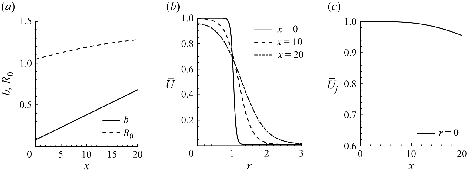
 M=2.24
 Md=2.0
 (a)
 b
 R0
 (b)
 x
 (c)
 U¯j
 r=0

 (a
 c
 e
 g)
 (b
 d
 f
 h)
 (a
 b)
 (c
 d)
 (e
 f)
 (g
 h)

 Δαn=αn+1−αn
 n=1−7

 (a)
 ϵ¯κn
 x
 (b)
 ϵsA^n
 x
 Δp=0.065
 (b)
 (a)

 Φ^n,N
 Δp=0.065

 r=0
 (a
 e)
 (f)

 M=2.24
 Md=2.0
 (a
 b)
 x=2
 (c
 d)
 x=8
 x=10
 (g
 h)
 x=12
 r=0
 r⩾1

 (a)
 ϵs2u00
 (b)
 ϵs2θ00
 (c)
 ϵs2ϵ¯v00

 (a
 c)
 (d
 f)
 m=2
 n=1
 (g
 i)
 m=2
 n=1
 (j
 l)

 a
 c
 b
 d
 ps
 a
 b
 c
 d
 k
 sk

 (a)
 r=0
 (b)
 r=0.5
 (c)
 r=0.9
 Δp=0.065

 a
 b
 r=0
 Δp

 a
 c
 e
 g
 b
 d
 f
 h
 ps/Δp
 Δp
 a
 b
 c
 d
 Δp=−0.01
 e
 f
 Δp=−0.05
 g
 h
 Δp=−0.1

 s1
 |Δp|
 s1=4+245(Δp)2
 s1=4+115(Δp)2
 M=2.24
 s1=2.64+32(Δp)2
 s1=2.64+20(Δp)2
 M=1.67

 Δp
 90%

 Md=1.0
 M
 (a
 b)
 M=1.16
 (c
 d)
 M=1.19
 (e
 f)
 M=1.22
 (g
 h)
 M=1.40
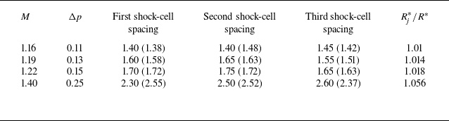
 M
 Md=1.0

 s1
 M
 Md=1.0
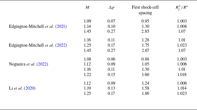
 Md=1.0

 (a)
 (Md=1.0)
 M=1.19
 (b)


