Introduction

Modeling ice sheets has become more important as well as more practical for a number of reasons. As more and more field data on the configuration of present-day ice sheets are accumulated, the important boundary conditions defining ice-sheet behavior become available. At the same time, the increasing body of information requires more and more sophisticated models adequately to depict reality. Small-scale features with important dynamic consequences, such as ice streams, require modeling on widely varying spatial and temporal scales (Reference MahaffyMahaffy, 1976; Reference JenssenJenssen, 1977; Reference OerlemansOerlemans, 1982).

Assessment of the present condition and future response of major existing ice sheets requires a time-dependent solution. This solution must allow variation of such major controlling influences as the mass balance, the temperature-dependence of the ice hardness, the variations in bed coupling, and the deformation of the bedrock itself. Changes in the bed coupling should be able to reflect both spatial and temporal variations produced by internal effects such as accumulating melt water at the bed, as well as externally produced effects due to changing climate.

Reconstructions of paleo-ice sheets, both as steady-state and time-dependent solutions, allow greater insight into the processes controlling stability and decay of present-day ice sheets. At the same time, reconstructions provide a window through which glacial geologists can refine their interpretations of glacial indicators, thereby providing more accurate descriptions of the environment of the past. As input to atmospheric models, these reconstructions allow a clearer picture of the climate in the past, and perhaps of the driving forces behind climate change in the past and future. Ultimately, a predictive model capable of modeling future glaciations will be both necessary and possible.

As a step towards this process, we present here a model of glacier dynamics that we feel has several advantages over many of the current models in use. The model presented here consists of a solution of the two-dimensional continuity equation for mass flow. The solution is obtained using a finite-element technique which builds upon previous work with a flow-band model (Reference Fastook, Van der Veen and OerlemansFastook, 1987).

The finite-element formulation as an equation solver has several advantages over more traditional finite-difference schemes. Specification of complex, non-uniform, and variable boundary conditions is easier to implement in a finite-element formulation, as the primary boundary condition, the boundary flux, occurs in a natural fashion in the element equations. Element boundaries, defined by nodal points, need not be rectangular or uniform in size. This allows more precise modeling of small dynamic features such as ice streams while allowing areas with relatively uniform properties such as an interior region of sheet flow to be economically modeled with fewer elements.

The two-dimensional nature of the solution frees us of many of the restrictions imposed by the one-dimensional flow-band model. In a flow-band model, flow directions must be defined externally by the modeler. In addition, these flow patterns must in general remain fixed during any time-dependent process that is being modeled. In flow-band models, two-dimensional effects are approximated by assuming uniform properties across the width of the flow band which itself is allowed to be non-uniform along the direction of flow. Clearly, during the growth or disintegration phase of an ice sheet, the flow patterns and catchment areas would not and should not be held fixed. In our current finite-element formulation, flow directions are a derived quantity and can vary in time as the configuration of the ice sheet changes.

Finite-element Formulation

The following details of this formulation are meant as an introduction to this model. This description is included as the modeling philosophy differs considerably from the usual stress-strain-rate solutions found in most finite-element models. The development of the formulation is based on techniques which can be found in greater detail in Reference Becker, Carey and OdenBecker and others (1981) and in Reference Fastook, Van der Veen and OerlemansFastook (1987).

The problem here is to solve the two-dimensional time-dependent continuity equation describing a map-plane model of ice flow. The solution to this equation represents ice-surface elevation, h, at (x,y) coordinates on a map of non-uniform bed elevations and accumulation/ablation rates, a(x,y). Boundary conditions may include either a specified ice thickness, H, along a boundary or a specified ice flux through a boundary. A finite-element solution is implemented using a Galerkin method which is described in Reference Becker, Carey and OdenBecker and others (1981).

The continuity equation for the model can be written

From a physical interpretation, the flux at a point (x,y) in the plane is given as the product of ice thickness and column-averaged velocity, U, while the finite-element method requires the expression of the flux-like variable as proportional to the surface slope. Hence, the flux is given in a constitutive equation as

The column-averaged velocity can be written as a combination of sliding and internal deformation (flow) proportional to the areal fraction of the bed melted:

It should be noted that the parameter / is basically unknown for both present and past ice sheets. An estimate of / for paleo-ice sheets can be obtained from glacial erosion patterns (Reference Hughes, Denton and HughesHughes, 1981). For present ice sheets, / can be estimated from considerations of the pressure-melting point, measurements by radar echo-sounding, and from the existence of ice streams (Reference Drewry, Gardner and ScogingDrewry, 1983). At present there is considerable controversy over the nature of the sliding law. In this model we use a simple sliding relationship dependent upon melting and regelation of ice flowing over bedrock obstacles (Reference WeertmanWeertman, 1964), although any sliding relationship relating velocity to surface slope could be used. The sliding velocity is given by

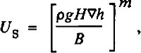
and the flow velocity (Reference GlenGlen, 1955; Reference WeertmanWeertman, 1957) is given by

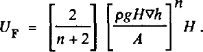
Neither of these formulations includes longitudinal forces and hence are only approximate. However, because of the generality and flexibility of the finite-element method, any “law” relating column-average velocity and surface slope can be used, allowing for future improvements as theory dictates. In the model,∇h is calculated at the centroid of each element by using the finite-element shape functions and their derivatives as interpolating functions.

The proportionality constant k(x,y) of equation (2) can be obtained by combining Equations (2), (3), (4), and (5) which results in

Solution of this non-linear problem can proceed by an iterative solution to the corresponding linearized problem. Initially k(x,y) is assumed to be uniform over the domain of the problem. A solution for H, the ice thickness, (and hence also for h, the surface elevation related through the bedrock elevation) can be found. From this solution, a new k(x,y) can be constructed from equation (6), and a new solution can be found. This process is repeated until the solution converges (i.e. the thickness stops changing). The rate of convergence is dependent on the initial uniform value given to k(x,y).

The application of the finite-element method starts With

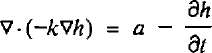
which results from manipulation of the continuity and constitutive equations. This form of the equation is very difficult to solve because the equation must be satisfied at every point in the domain of the problem.

The finite-element method allows for a re-formulation of the problem via the principle of weighted residuals, thereby producing an equation which represents the same physical principles, but in a more average sense. This residual form of the equation takes the form

This formulation of the problem is more amenable to solution, because, while it is satisfied over the whole region of the domain R of the problem, it is also satisfied over any smaller region Ω of the domain R. A grid can then be applied to the domain R which divides the region into smaller units called elements. An equation identical to equation (8) can then be written for an element Ω of R which is called the element equation.

The equation for each element can be manipulated using Gauss’ theorem which results in the symmetric formulation of equation (8) for the element Ω

where kdh/dn is as the normal component of the flux crossing the boundary of the element Ω. When the solution for the many elements is combined to recreate the original domain R, these terms will exactly cancel for adjacent elements, so that their only contribution will be for elements with no neighbors, i.e. the boundary of the domain R. Hence, the specification of fluxes along boundaries to the domain occurs naturally in the formulation of the problem.

The finite-element method is then applied to the resulting element equation. The unknown h and the trial function y are replaced by finite summations over basis functions with coefficients equal to their values at the four nodal points used to define the shape of the quadrilateral elements. Combining the various element equations relating the nodal values of the unknown h, one obtains a global matrix equation of the form

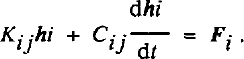
The vector h _i• represents the unknown ice elevations at each of the nodal points defining the domain R. The elements of K_ij and C_ij, and F_i are integrals of simple linear functions and their products so that the integrations can be performed analytically or with a simple numerical scheme (nine-point Gaussian integration is used here). For the steady-state solution, the time-derivative term is zero and equation (10) is simply

which can be solved for the unknown h’s by standard methods.

For the time-dependent solution, an unconditionally stable backward difference scheme is used where the time derivative is approximated by

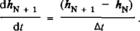
Here, the vector and matrix indices have been dropped and the N and N + 1 represent the N^th and N + 1^st time steps. Replacing the time derivative in equation (10) and solving for the solution vector at the N + 1^s time step, one obtains

where I is the identity matrix. Thus, given an initial surface for an ice sheet (the h _N vector) and a new set of boundary conditions (the F _N+1 vector), a solution for the new ice-sheet surface at the N+1^st time step is obtained.

It is convenient to use the backward-difference scheme because of its inherent unconditional stability. Also, while the order of accuracy of the backward-difference scheme is 0(k + h²) and other numerical schemes of a higher order of accuracy could have been used, the backward-difference scheme does not alter the method of solution which results from the implementation of the finite-element method. A higher-order scheme, such as a Crank-Nicholson or leapfrog scheme, would be computationally difficult to install in the model. Also, the lower order of accuracy is not apparent until time steps greater than 200 years are modeled.

Results and Modeling Experiments

Three modeling experiments are described in this section. As discussed in the finite-element formulation section, the domain of the problem must be divided into elements via a grid. In each of the modeling experiments, a square domain 1000 km on a side is defined by 225 nodal points in a rectangular arrangement which form 196 elements. The following experiments have been chosen to demonstrate some of the strengths of the finite-element model.

The first experiment depicts flow over and around a series of obstacles, in this case a set of intersecting mountain ridges. Figure 1 shows the bedrock configuration for this experiment, a uniform flat bed at sea-level with two ridges 2000 m high approximately 600 km long running from the top of the figure to the bottom, separated by approximately 100 km at their bases and approximately 500 km at their peaks. Top and bottom boundaries are specified to allow no flux to cross, while the right-hand boundary has a specified flux of 1.0 χ 10⁵m²/year. The accumulation rate over the domain is zero everywhere, so that the ice margin advances from right to left, eventually over-riding the ridges and covering the entire domain. Velocity vectors are shown for an intermediate time (17 000 years) when the right-hand ridges have been over-run, but the ice has not crested the left-hand ridge. The magnitude of the vectors is indicated by the horizontal line at the top of the figure, which represents a velocity of 333 m/year. Typical velocities along the right-hand margin are in the neighborhood of 20 m/year, with maximum velocities reaching approximately 50 m/year in the thick ice (3000 m) filling the valley and in the thinner ice (1500 m) along the crest of the over-ridden ridge. Figure 2 shows surface-elevation contours for this time period, again with velocity vectors superimposed. The very strong topographic control of the flow direction is clear in this figure, with velocity vectors in the valley region being deflected by as much as 65° from the unimpeded direction of flow. As both ridges are over-ridden, the topographic control declines with deflections lowering to approximately 15° in the valley region.

Fig. 1.

The bedrock configuration for flow around obstacles, a uniform flat bed at sea-level with two ridges 2000 m high approximately 600 km long running from the top of the figure to the bottom, separated by approximately 100 km at their bases and approximately 500 km at their peaks, with superimposed velocity vectors for the configuration at 16 000 years.

Fig. 2.

Surface-elevation contours for 17 000 years, again with velocity vectors superimposed.

The second modeling experiment is a simulation demonstrating the effects of a changing mass-balance pattern. Figure 3 shows steady-state surface-elevation contours and velocity vectors for a symmetric accumulation distribution. The domain in this experiment is a square 2000 km on a side. The accumulation rate is 0.4 m/year over a region covering approximately 90 000 km² centered on the figure coordinates (0.0, 0.0). Everywhere outside this region the ablation rate is –0.4 m/year, resulting in a steady-state ice sheet with a diameter of approximately 1200 km. Note the velocity attains a maximum value of 30 m/year approximately 400 km from the center of the ice sheet, declining as the ice approaches the margin.

Fig. 3.

Steady-state surface-elevation contours and velocity vectors for a symmetric accumulation distribution.

Beginning with this configuration, the accumulation rate over the left-hand side of the ice sheet is reduced by 95% (0.2 m/year for X ≤ 0.0, 0.4 m/year for X > 0.0). Figure 4 shows time-dependent profiles along the Y = 0.0 transect through the ice sheet at 1000 year intervals, depicting the response to the changed accumulation pattern. Thinning near the left-hand margin is 0.185 m/year during the first 1000 year interval, and increases gradually to 0.29 m/year as the ice-sheet margin retreats approximately 140 km in this 8000 year simulation. Thinning at interior points also begins near 0.185 m/year, but instead declines as a new steady-state configuration is attained between 7000 and 8000 years.

Fig. 4.

Time-dependent profiles along the Y = 0.0 transect through the ice sheet at 1000 year intervals, depicting the response to the changed accumulation pattern.

Figure 5 shows the steady-state surface-elevation contours and velocity vectors for the asymmetric accumulation pattern. Note the significantly lowered dome, which is displaced approximately 130 km to the right, as well as the marked asymmetry in the velocity magnitudes. While the right-hand side velocities remain essentially unchanged in magnitude, velocities in the lowered accumulation region are reduced by 60% to as little as 10 m/year.

Fig. 5.

Steady-state surface-elevation contours and velocity vectors for the asymmetric accumulation pattern.

The final modeling experiment is a simulation of the time-dependent evolution of an ice stream. In this simulation, an ice sheet with a fully frozen bed provides the initial configuration, and the response is monitored as a part of this ice sheet is decoupled from the bed by allowing sliding. The domain is again a 2000 km square, with the central accumulation rate adjusted so that the ice sheet just reaches the boundaries of the domain. Ablation around this central region insures that ice velocities are close to zero along this margin. Figure 6 shows the steady-state surface-elevation contours and velocity vectors for this initial configuration. A channel 400 km wide and 500 m deep extending from the center of the ice sheet to the right-hand margin provides a slight degree of asymmetry to this initial configuration. Velocities in this channel reach 100 m/year, twice the value in the region of the flat bed, and do not decline to zero at the domain boundary, indicating a flux across the grounding line which would either produce an ice shelf or calving icebergs. A slight shift of the central dome to the left with accompanying decline in surface slope on the right is all that this channel produces.

Fig. 6.

Steady-state surface-elevation contours and velocity vectors for no sliding. A channel 400 km wide and 500 m deep extending from the center of the ice sheet to the right-hand margin provides a slight degree of asymmetry to this initial configuration.

Beginning with this configuration, all bedrock below sea-level is assumed to thaw, thereby allowing sliding (Reference WeertmanWeertman, 1964) as the bedrock obstacles are drowned by the increased water layer. Figure 7 shows time-dependent profiles along the Y = 0.0 transect through the ice sheet at 200 year intervals for the first 1000 years, and 1000 year intervals thereafter, depicting the response to the changed basal conditions. Initial thinning rates are very high, approaching 1 m/year at the head of the ice stream. These rates decline rapidly and a new steady-state configuration is attained in approximately 5000 years. In this time the dome elevation lowers by 450 m and shifts over 200 km away from the ice stream.

Fig. 7.

Time-dependent profiles along the Y = 0.0 transect through the ice sheet at 200 year intervals for the first 1000 years, and 1000 year intervals thereafter, depicting the response to the initiation of sliding in the channel.

Figure 8 shows surface-elevation contours and velocity vectors for the new steady-state configuration with sliding in the channel. Note the general retreat of the margins even far from the ice stream as much more of the mass balance flows out through the thawed channel. Strong down-draw, a marked concavity in the contours, and strong converging flow into the ice stream is evident over the region of thawed bed. Velocity along the thawed channel increases along its length, attaining sliding velocities of over 680 m/year at the grounding line. This increase in ice flux of more than a factor of 5 would certainly affect the existence of any ice shelf along this margin. The time-dependent profiles show the generally faster response of the ice sheet to a change in basal conditions when compared to its response to change in mass balance.

Fig. 8.

Surface-elevation contours and velocity vectors for the new steady-state configuration with sliding in the channel.

Conclusion

These experiments demonstrate the ability of the finite-element formulation to model properly the effects of a non-uniform bedrock configuration, a changing and non-uniform mass-balance pattern, and the formation of an ice stream. It is important to note that this finite-element formulation also allows for a non-uniform sliding or flow-law parameter as well as for a non-uniform column-averaged ice density. It is also possible to allow all of the properties to be spatially non-uniform or temporally variable in the same experiment whether it is a steady-state or time-dependent application. The model is quite capable of handling complex situations where the flow directions change radically.

The full potential of the flexibility that this model affords is still being explored. Future improvements include the ability to handle specified flux boundary conditions and perhaps mixed boundary conditions, as well as an isostasy criterion for the bed depression. In the model presented here the boundary is fixed spatially, and relaxing this requirement to allow margin positions to respond to changing boundary conditions is being explored.