1 Introduction
Waves accompanied by a steadily translating disturbance along a straight trajectory in calm water confined within a Kelvin wedge with a half-angle
 $\unicode[STIX]{x1D6FE}_{0}=19^{\circ }28^{\prime }$
are of both theoretical and practical significance (Wehausen Reference Wehausen1973). The stationary phase analysis to the dispersion relation shows that the open dispersion curve is divided by an inflexion into two branches corresponding to transverse waves and divergent waves, respectively (Lighthill Reference Lighthill1978). Furthermore, more complicated ship waves are investigated, including nonlinear free-surface flows (Forbes Reference Forbes1989; Pethiyagoda, McCue & Moroney Reference Pethiyagoda, McCue and Moroney2014a
; Pethiyagoda et al.
Reference Pethiyagoda, McCue, Moroney and Back2014b
), the presence of shear current (Ellingsen Reference Ellingsen2014; Li & Ellingsen Reference Li and Ellingsen2016), the surface tension effect (Moisy & Rabaud Reference Moisy and Rabaud2014; Liang & Chen Reference Liang and Chen2018), the bottom topography (Grue Reference Grue2017), etc. The fundamental solution to this steady ship-wave problem (also referred to as the ship-wave Green function) represents the flow induced by a point source/sink with unit strength translating steadily along a rectilinear path in calm water, and it is an essential building block to constructing the boundary integral equation to represent the free-surface flow by a travelling ship hull within the linear potential theory (Brard Reference Brard1972; Guével, Vaussy & Kobus Reference Guével, Vaussy and Kobus1974; Noblesse, Huang & Yang Reference Noblesse, Huang and Yang2013). The expression of the ship-wave Green function in the form of a double Fourier integral is collected by Wehausen & Laitone (Reference Wehausen and Laitone1960).
To evaluate the ship-wave Green function efficiently and with sufficient accuracy, the double Fourier integral is usually decomposed into a wave component dominant in the far field and a non-oscillatory local-flow component using Cauchy’s residue theorem (Noblesse Reference Noblesse1977, Reference Noblesse1981; Newman Reference Newman1987). The local-flow component expressed as a single integral of a complex exponential-integral function can be further approximated analytically (Noblesse et al.
Reference Noblesse, Delhommeau, Huang and Yang2011). For the wave component, the asymptotic approximations due to Kelvin (Reference Kelvin1887), Havelock (Reference Havelock1908) and Peters (Reference Peters1949) are applicable for the flow-field point located inside, at and outside the Kelvin wedge, respectively. Inside and at the cusp of the Kelvin wedge, waves decay as
 $R^{-1/2}$
and
 $R^{-1/3}$
, respectively, where
 $R$
is the horizontal distance from the disturbance, whereas waves decay exponentially outside the Kelvin wedge. Besides the approximations given by Kelvin, Havelock and Peters, Ursell (Reference Ursell1960) gave an approximation associated with the Airy function and its derivative which is uniformly valid inside, at and outside the cusp, and he also reported the singular behaviour of waves generated by a concentrated pressure point. Ursell’s approximation is based on an extension of the method of steepest descent which is also referred to as the Chester–Friedman–Ursell (CFU) approximation (Chester, Friedman & Ursell Reference Chester, Friedman and Ursell1957). Lustri & Chapman (Reference Lustri and Chapman2013) studied the asymptotic behaviours at a low speed. Recently, Wu et al. (Reference Wu, He, Zhu and Noblesse2018) proposed another alternative uniform approximation which combines the expressions given by Kelvin, Havelock and Peters, and thus it is referred to as the Kelvin–Havelock–Peters (KHP) approximation. Despite the fact that the KHP approximation is not as accurate as Ursell’s approximation, yet it has a simple form consisting of elementary functions only, and it has been used to investigate the influence of the Froude number on the wave pattern (Wu et al.
Reference Wu, He, Liang and Noblesse2019). All of these efforts give an insight into the behaviours of the ship-wave Green function. Similar to the behaviours of waves generated by a pressure point (Ursell Reference Ursell1960), both numerical evaluation and asymptotic approximation show that very short and steep divergent waves exist when both source and flow-field points are on the free surface. Furthermore, the fundamental solution is singular as the flow-field point approaches the track of the source point (Clarisse & Newman Reference Clarisse and Newman1994; Chen & Wu Reference Chen and Wu2001; Motygin Reference Motygin2017). These unphysical behaviours partly stem from an ignorance of viscous effects.
Introducing viscous damping in water waves could be traced back to Lamb (Reference Lamb1932). Longuet-Higgins (Reference Longuet-Higgins1992) assumed that the vortical boundary layer is attached to the free surface, and introduced the Helmholtz decomposition to divide the velocity into irrotational and vortical components. Joseph (Reference Joseph2003) formulated the viscous potential flow equations for compressible fluids, and the phrase ‘viscous potential flow’ was proposed. Joseph & Wang (Reference Joseph and Wang2004) developed a viscous corrected viscous potential flow theory, and investigated the decay rate of progressive gravity waves in comparison with Lamb’s exact solution. Dias, Dyachenko & Zakharov (Reference Dias, Dyachenko and Zakharov2008) made a systematic investigation into the effect of viscosity on free-surface waves in deep water, and a weakly damped free-surface flow theory was established. However, their study made use of the streamfunction, and thus it is limited to the two-dimensional problem. Then, Dutykh & Dias (Reference Dutykh and Dias2007) generalized Dias et al.’s work to three dimensions, and a general joint Fourier–Laplace transform was applied to treat the governing equation and boundary conditions. However, it was suggested that the ‘molecular’ kinematic viscosity in the weakly damped free-surface flow
 $\unicode[STIX]{x1D708}=1.0\times 10^{-6}~\text{m}^{2}~\text{s}^{-1}$
was too small, and it is typically taken as
 $\unicode[STIX]{x1D708}=1.0\times 10^{-4}\sim 1.0\times 10^{-3}~\text{m}^{2}~\text{s}^{-1}$
to account for the effective ‘eddy’ viscosity (Dias et al.
Reference Dias, Dyachenko and Zakharov2008; Horsley & Forbes Reference Horsley and Forbes2013).
In this paper, three-dimensional free-surface waves generated by a translating source with a constant speed, accounting for viscous effects are considered. The fluid is assumed to be incompressible, and the surface tension effect is disregarded. Viscous effects are accounted for based on the weakly damped free-surface flow theory (Dutykh & Dias Reference Dutykh and Dias2007; Dias et al. Reference Dias, Dyachenko and Zakharov2008). The three-dimensional steady ship-wave problem accounting for viscous effects is pioneered by Cumberbatch (Reference Cumberbatch1965), and it shows that divergent waves are severely damped by viscous effects resulting in a finite wave amplitude along the track. Then, subsequent studies are carried out. Lu & Chwang (Reference Lu and Chwang2005, Reference Lu and Chwang2007) studied the interfacial viscous ship waves in a system of two semi-infinite fluids with different densities, and asymptotic approximations valid in different flow regions are presented. Recently, Dai (Reference Dai and Kashiwagi2014) gave a uniform asymptotic expression for the interfacial viscous ship wave problem based on the CFU approximation (Chester et al. Reference Chester, Friedman and Ursell1957).
Unlike existing studies and the authors’ previous work (Liang & Chen Reference Liang and Chen2018) in which the analysis of the pattern of iso-phase lines is conducted via phase relations, the emphasis of the present paper is placed on the influence of viscous effects on the amplitude of the fundamental solution for ship waves. Due to the presence of viscosity, the analysis becomes more complicated. Besides the technique to evaluate the double Fourier integral efficiently and accurately, five types of asymptotic approximations – including three classical non-uniform asymptotic approximations (Kelvin Reference Kelvin1887; Havelock Reference Havelock1908; Peters Reference Peters1949) and two uniform asymptotic approximations (CFU approximation (Chester et al. Reference Chester, Friedman and Ursell1957) and KHP approximation (Wu et al. Reference Wu, He, Zhu and Noblesse2018)) – are made to obtain analytical expressions in the form of elementary functions. These analytical expressions explicitly reveal the underlying physics associated with the viscous-ship-wave Green function and illustrate how viscosity affects the amplitude of waves.
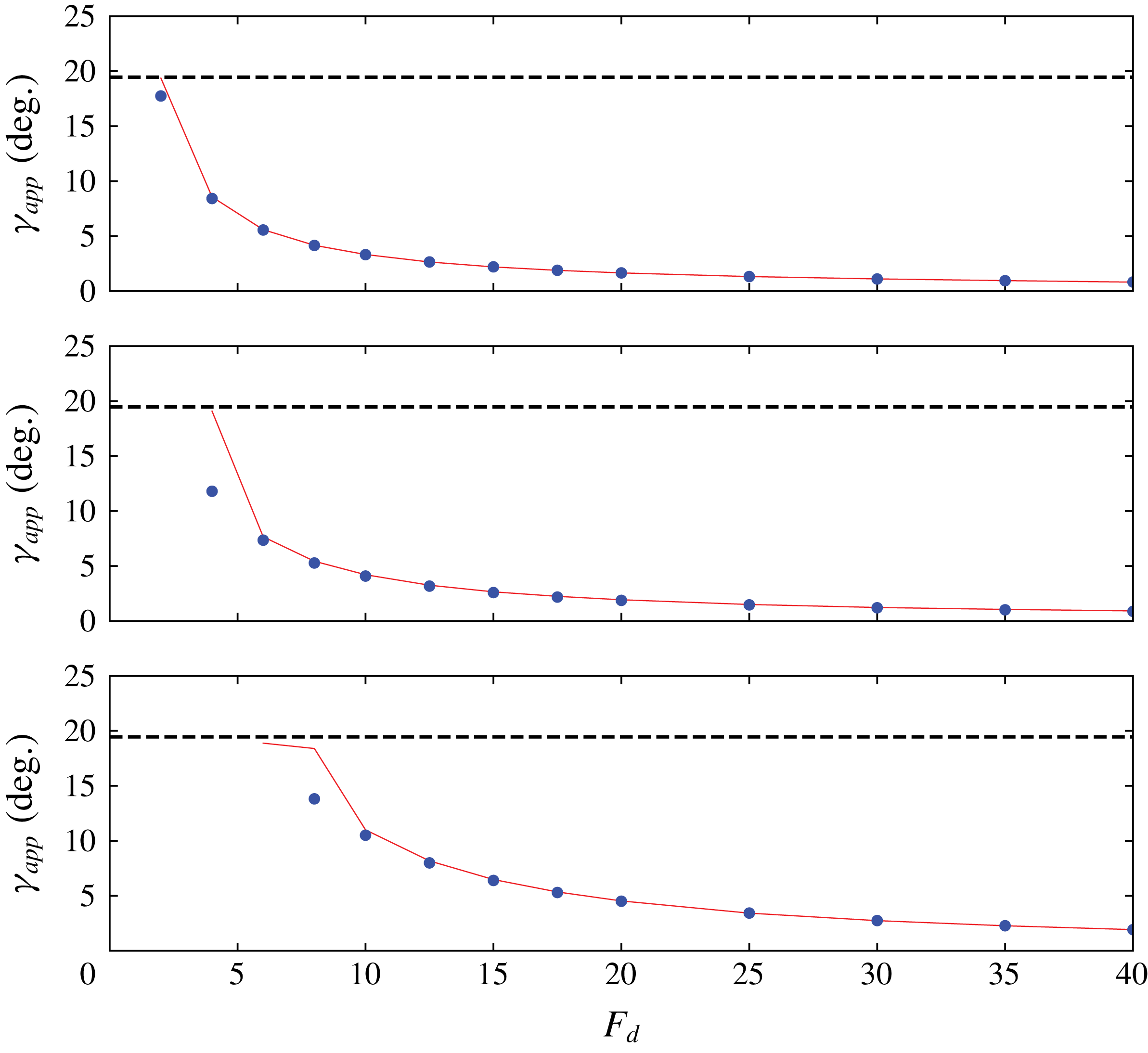
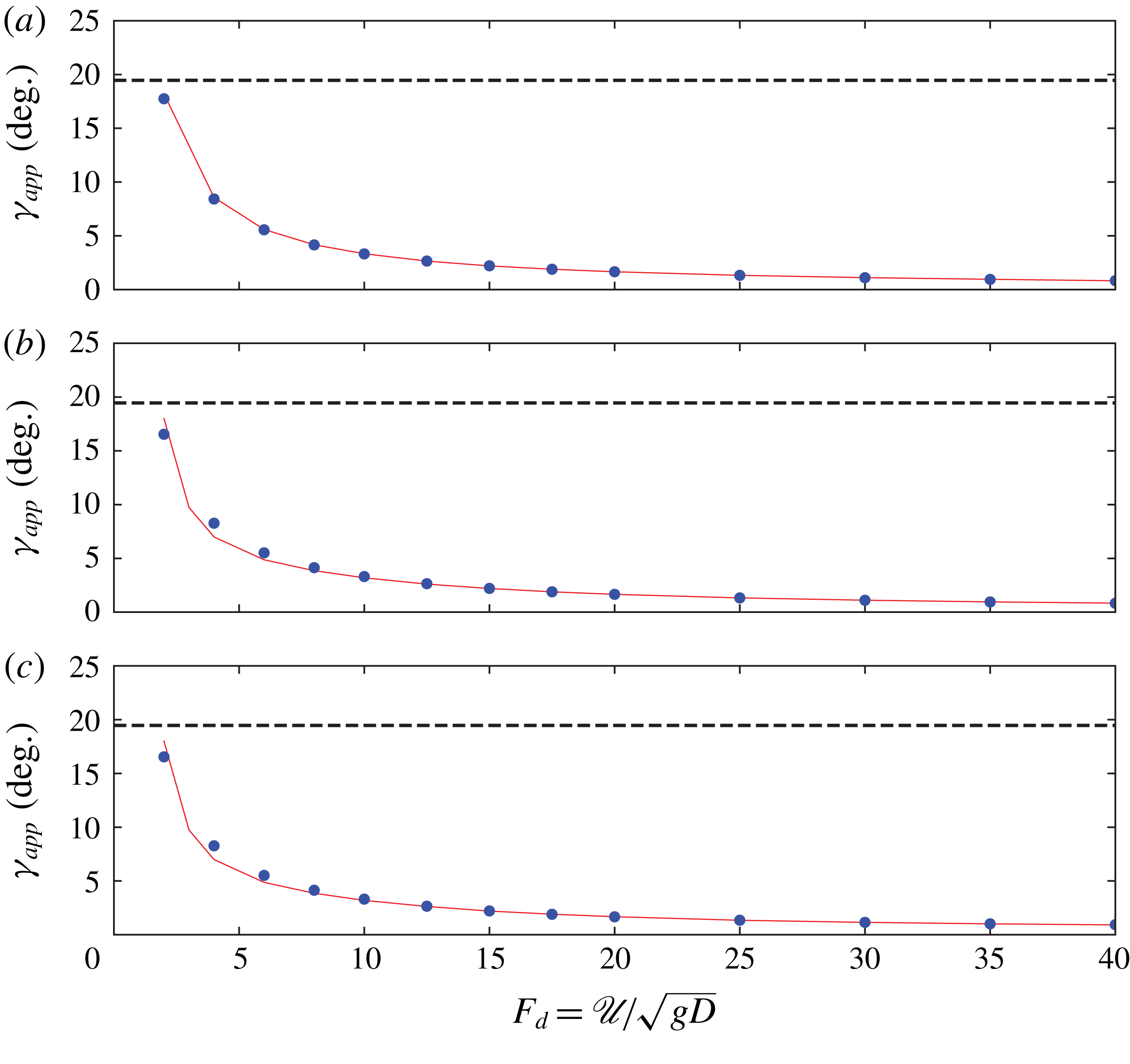
The layout of the paper is as follows. An explicit expression for the fundamental solution is first of all formulated in § 2, and the corresponding efficient and accurate evaluation method is described in § 3. To look into the flow physics of the viscous-ship-wave Green function, classical asymptotic approximations, which are valid inside, at and outside the Kelvin wedge due to Kelvin, Havelock and Peters, are used to convert the integral to algebraic expressions in § 4. The physical behaviour near the track is revealed. Due to the fact that Kelvin’s and Peters’ approximations are singular at the cusp, the uniform approximations based on the CFU approximation and KHP approximation are set forth in § 5. In § 6, numerical evaluation and asymptotic approximation of the viscous-ship-wave Green function are made and it is evident that the incorporation of viscous effects makes free-surface waves physically realistic – the singular behaviour is eliminated and rapid oscillations near the track due to divergent waves are severely damped. Then, in § 7, the apparent wake angle of free-surface waves generated by a translating source is investigated. It is demonstrated that the apparent wake angle is associated with both
 $\mathscr{U}^{-1}$
and
 $\mathscr{U}^{-2}$
, where
 $\mathscr{U}$
is the travelling speed of the source. In addition, viscous effects widen the region near the track without divergent waves. Finally, conclusions drawn from the present study are summarized in § 8.
2 Viscous-ship-wave Green function
The viscous-ship-wave Green function is now considered. A frame of reference
 $OXYZ$
translating with the disturbance at a constant speed
 $\mathscr{U}$
in the direction of the negative
 $X$
-axis is defined with the
 $OXY$
plane coinciding with the undisturbed free surface and
 $Z$
-axis orienting positively upward. Here, the translating speed
 $\mathscr{U}$
and the gravitational acceleration
 $g$
are used to define the non-dimensional coordinates
 $(x,y,z)$
, and velocity potential
 $\unicode[STIX]{x1D719}$
with respect to
 $g/\mathscr{U}^{2}$
and
 $g/\mathscr{U}^{3}$
, respectively. By starting from the linearized incompressible Navier–Stokes equations and applying the Helmholtz decomposition theorem, the linear free-surface boundary condition accounting for viscous effects can be obtained (for details refer to appendix A),
 $$\begin{eqnarray}\frac{\unicode[STIX]{x2202}^{2}\unicode[STIX]{x1D719}}{\unicode[STIX]{x2202}x^{2}}+\frac{\unicode[STIX]{x2202}\unicode[STIX]{x1D719}}{\unicode[STIX]{x2202}z}+4\unicode[STIX]{x1D716}\frac{\unicode[STIX]{x2202}^{3}\unicode[STIX]{x1D719}}{\unicode[STIX]{x2202}x\unicode[STIX]{x2202}z^{2}}=0,\quad \text{on}~z=0,\end{eqnarray}$$
where the non-dimensional parameter
 $\unicode[STIX]{x1D716}$
associated with viscous effects is defined as
 $$\begin{eqnarray}\unicode[STIX]{x1D716}=g\unicode[STIX]{x1D708}/\mathscr{U}^{3},\end{eqnarray}$$
where
 $\unicode[STIX]{x1D708}$
denotes the kinematic fluid viscosity, and the molecular viscosity coefficient is
 $\unicode[STIX]{x1D708}=10^{-6}~\text{m}^{2}~\text{s}^{-1}$
. Suppose that a source with strength
 $\unicode[STIX]{x1D70E}$
is located at
 $(\unicode[STIX]{x1D709},\unicode[STIX]{x1D702},\unicode[STIX]{x1D701})$
, and the corresponding potential is
 $\unicode[STIX]{x1D719}=\unicode[STIX]{x1D70E}G$
, where
 $G$
means the source potential with unit strength (also referred to as the Green function). The governing equation at a flow-field point
 $(x,y,z)$
in the fluid domain for the unit source potential
 $G$
beneath a free surface is
 $$\begin{eqnarray}\unicode[STIX]{x1D6FB}^{2}G=\unicode[STIX]{x1D6FF}(x-\unicode[STIX]{x1D709},y-\unicode[STIX]{x1D702},z-\unicode[STIX]{x1D701}),\quad \text{with}~z\leqslant 0,\end{eqnarray}$$
where
 $\unicode[STIX]{x1D6FF}$
means the Dirac delta function. The fundamental solution to the governing equation (2.3) satisfying the free-surface boundary condition (2.1) for the source potential can be expressed in the form of
 $$\begin{eqnarray}4\unicode[STIX]{x03C0}G=-\frac{1}{r}+\frac{1}{r^{\prime }}+G^{F},\end{eqnarray}$$
where
 $r$
and
 $r^{\prime }$
are defined as
 $$\begin{eqnarray}r=\sqrt{(x-\unicode[STIX]{x1D709})^{2}+(y-\unicode[STIX]{x1D702})^{2}+(z-\unicode[STIX]{x1D701})^{2}}\quad \text{and}\quad r^{\prime }=\sqrt{(x-\unicode[STIX]{x1D709})^{2}+(y-\unicode[STIX]{x1D702})^{2}+(z+\unicode[STIX]{x1D701})^{2}},\end{eqnarray}$$
and
 $G^{F}$
denotes the potential due to the free-surface disturbance. Without loss of generality, we suppose that the source point is located at a point (
 $z\leqslant 0$
) along the
 $z$
-axis which means that
 $\unicode[STIX]{x1D709}=0$
and
 $\unicode[STIX]{x1D702}=0$
. In (2.4), expressions
 $1/r$
and
 $1/r^{\prime }$
can be represented in the form of double Fourier integrals (Bronshtein et al.
Reference Bronshtein, Semendyayev, Musiol and Muehlig2003)
 $$\begin{eqnarray}\displaystyle & \displaystyle \frac{1}{r}=\frac{1}{2\unicode[STIX]{x03C0}}\int _{-\infty }^{\infty }\int _{-\infty }^{\infty }\frac{1}{k}\text{e}^{-k|z-\unicode[STIX]{x1D701}|+\text{i}(\unicode[STIX]{x1D6FC}x+\unicode[STIX]{x1D6FD}y)}\,\text{d}\unicode[STIX]{x1D6FC}\,\text{d}\unicode[STIX]{x1D6FD}, & \displaystyle\end{eqnarray}$$
 $$\begin{eqnarray}\displaystyle & \displaystyle \frac{1}{r^{\prime }}=\frac{1}{2\unicode[STIX]{x03C0}}\int _{-\infty }^{\infty }\int _{-\infty }^{\infty }\frac{1}{k}\text{e}^{k(z+\unicode[STIX]{x1D701})+\text{i}(\unicode[STIX]{x1D6FC}x+\unicode[STIX]{x1D6FD}y)}\,\text{d}\unicode[STIX]{x1D6FC}\,\text{d}\unicode[STIX]{x1D6FD}, & \displaystyle\end{eqnarray}$$
 $(\unicode[STIX]{x1D6FC},\unicode[STIX]{x1D6FD})$
Fourier plane with
 $(\unicode[STIX]{x1D6FC},\unicode[STIX]{x1D6FD})=k(\cos \unicode[STIX]{x1D703},\sin \unicode[STIX]{x1D703})$
. By introducing the Fourier transform
 $$\begin{eqnarray}\widetilde{G}(\unicode[STIX]{x1D6FC},\unicode[STIX]{x1D6FD},z)=\int _{-\infty }^{\infty }\int _{-\infty }^{\infty }G(x,y,z)\text{e}^{-\text{i}(\unicode[STIX]{x1D6FC}x+\unicode[STIX]{x1D6FD}y)}\,\text{d}x\,\text{d}y,\end{eqnarray}$$
to the free-surface boundary condition given by (2.1) and the governing equation (2.3) as carried out in Liang & Chen (Reference Liang and Chen2017), we have
 $$\begin{eqnarray}\displaystyle & \displaystyle \widetilde{G}^{F}(\unicode[STIX]{x1D6FC},\unicode[STIX]{x1D6FD},z)=A(\unicode[STIX]{x1D6FC},\unicode[STIX]{x1D6FD})\text{e}^{kz}, & \displaystyle\end{eqnarray}$$
 $$\begin{eqnarray}\displaystyle & \displaystyle -2\unicode[STIX]{x03C0}\frac{\text{e}^{-k|\unicode[STIX]{x1D701}|}}{k}(-\unicode[STIX]{x1D6FC}^{2}-k+4\text{i}\unicode[STIX]{x1D716}\unicode[STIX]{x1D6FC}k^{2})+\left(2\unicode[STIX]{x03C0}\frac{\text{e}^{k\unicode[STIX]{x1D701}}}{k}+A\right)(-\unicode[STIX]{x1D6FC}^{2}+k+4\text{i}\unicode[STIX]{x1D716}\unicode[STIX]{x1D6FC}k^{2})=0. & \displaystyle\end{eqnarray}$$
By making the inverse Fourier transform, we can obtain the free-surface term
 $G^{F}$
in the form of
 $$\begin{eqnarray}G^{F}=\frac{1}{\unicode[STIX]{x03C0}}\int _{-\infty }^{\infty }\int _{-\infty }^{\infty }\frac{1}{\mathscr{D}(\unicode[STIX]{x1D6FC},\unicode[STIX]{x1D6FD})}\text{e}^{k(z+\unicode[STIX]{x1D701})+\text{i}(\unicode[STIX]{x1D6FC}x+\unicode[STIX]{x1D6FD}y)}\,\text{d}\unicode[STIX]{x1D6FC}\,\text{d}\unicode[STIX]{x1D6FD},\end{eqnarray}$$
where the denominator
 $\mathscr{D}$
in (2.9) represents the dispersion function associated with the linear free-surface boundary condition (2.1), and the dispersion functions on the
 $\unicode[STIX]{x1D6FC}\unicode[STIX]{x1D6FD}$
and
 $k\unicode[STIX]{x1D703}$
Fourier planes are written as
 $$\begin{eqnarray}\displaystyle & \displaystyle \mathscr{D}(\unicode[STIX]{x1D6FC},\unicode[STIX]{x1D6FD})=\unicode[STIX]{x1D6FC}^{2}-\sqrt{\unicode[STIX]{x1D6FC}^{2}+\unicode[STIX]{x1D6FD}^{2}}-4\text{i}\unicode[STIX]{x1D716}\unicode[STIX]{x1D6FC}(\unicode[STIX]{x1D6FC}^{2}+\unicode[STIX]{x1D6FD}^{2}), & \displaystyle\end{eqnarray}$$
 $$\begin{eqnarray}\displaystyle & \displaystyle \mathscr{D}(k,\unicode[STIX]{x1D703})=k^{2}\cos ^{2}\unicode[STIX]{x1D703}-k-4\text{i}\unicode[STIX]{x1D716}k^{3}\cos \unicode[STIX]{x1D703}, & \displaystyle\end{eqnarray}$$
 $(\unicode[STIX]{x1D6FC},\unicode[STIX]{x1D6FD})=k(\cos \unicode[STIX]{x1D703},\sin \unicode[STIX]{x1D703})$
. In (2.10), viscous effects only contribute to the imaginary part of the dispersion function. Hence, viscous effects do not affect the profile of the free-surface wave pattern, but will attenuate the amplitude of waves. Due to the fact that viscous effects are associated with
 $k^{3}$
, they will have a tremendous influence on short waves with large wavenumbers. Then, expression (2.9) can be equivalently rewritten as
 $$\begin{eqnarray}G^{F}=\frac{2}{\unicode[STIX]{x03C0}}\text{Re}\int _{-\unicode[STIX]{x03C0}/2}^{\unicode[STIX]{x03C0}/2}\int _{0}^{\infty }\frac{1}{k\cos ^{2}\unicode[STIX]{x1D703}-1-4\text{i}\unicode[STIX]{x1D716}k^{2}\cos \unicode[STIX]{x1D703}}\text{e}^{k(z+\unicode[STIX]{x1D701})+\text{i}k(x\cos \unicode[STIX]{x1D703}+y\sin \unicode[STIX]{x1D703})}\,\text{d}k\,\text{d}\unicode[STIX]{x1D703}.\end{eqnarray}$$
By enforcing the dispersion equation
 $\mathscr{D}=0$
, we get two characteristic wavenumbers
 $$\begin{eqnarray}\displaystyle & \displaystyle k_{1}=\frac{2}{\cos ^{2}\unicode[STIX]{x1D703}+\sqrt{\cos ^{4}\unicode[STIX]{x1D703}-16\text{i}\unicode[STIX]{x1D716}\cos \unicode[STIX]{x1D703}}}=\frac{\cos ^{2}\unicode[STIX]{x1D703}-\sqrt{\cos ^{4}\unicode[STIX]{x1D703}-16\text{i}\unicode[STIX]{x1D716}\cos \unicode[STIX]{x1D703}}}{8\text{i}\unicode[STIX]{x1D716}\cos \unicode[STIX]{x1D703}}, & \displaystyle\end{eqnarray}$$
 $$\begin{eqnarray}\displaystyle & \displaystyle k_{2}=\frac{\cos ^{2}\unicode[STIX]{x1D703}+\sqrt{\cos ^{4}\unicode[STIX]{x1D703}-16\text{i}\unicode[STIX]{x1D716}\cos \unicode[STIX]{x1D703}}}{8\text{i}\unicode[STIX]{x1D716}\cos \unicode[STIX]{x1D703}}. & \displaystyle\end{eqnarray}$$
In the presence of viscous effects, the wavenumbers
 $k_{1}$
and
 $k_{2}$
are complex. Due to the fact that
 $\unicode[STIX]{x1D716}$
is a small parameter, the arguments of
 $k_{1}$
and
 $k_{2}$
are written as
 $$\begin{eqnarray}\unicode[STIX]{x1D6EC}_{1}=\arctan \left(\frac{4\unicode[STIX]{x1D716}}{\cos ^{3}\unicode[STIX]{x1D703}}\right)\quad \text{and}\quad \unicode[STIX]{x1D6EC}_{2}=-\unicode[STIX]{x03C0}+\arctan \left(\frac{\cos ^{3}\unicode[STIX]{x1D703}}{4\unicode[STIX]{x1D716}}\right),\end{eqnarray}$$
which indicates that
 $k_{1}$
is located in the first quadrant, while
 $k_{2}$
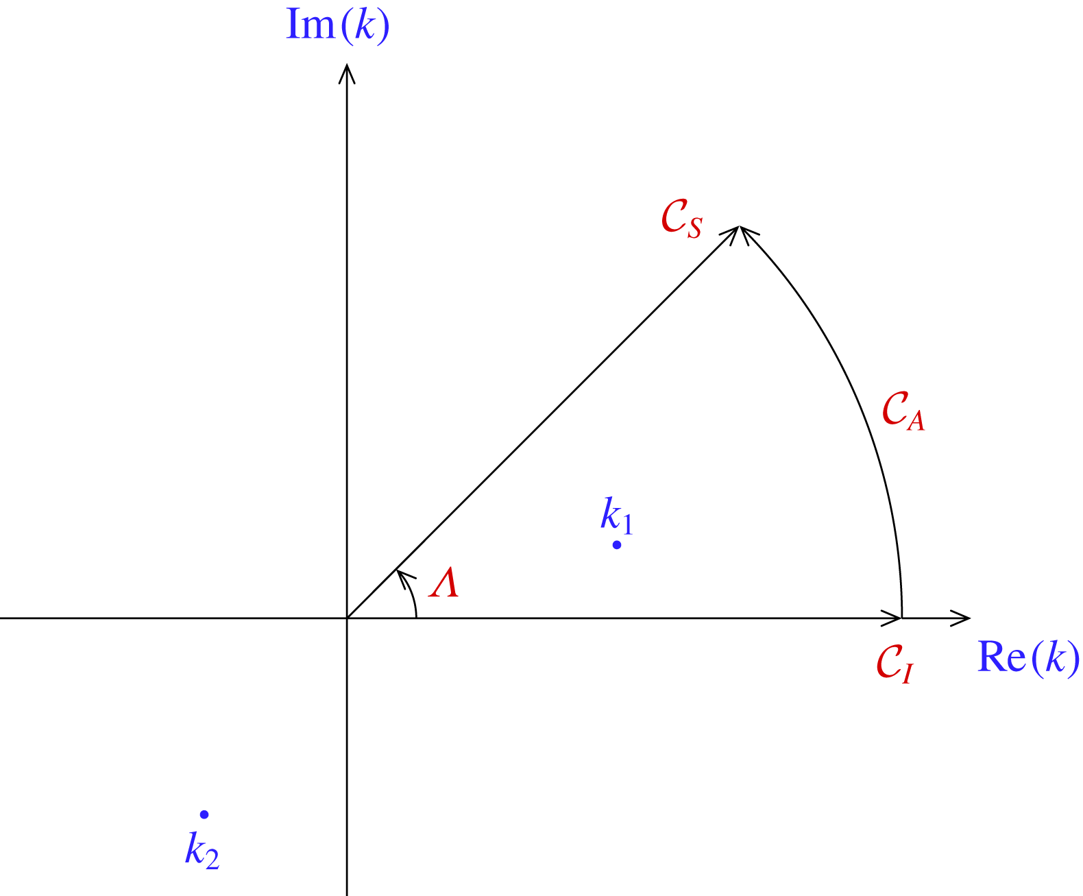
is in the third quadrant of the Fourier plane as shown in figure 1.
Sketch of deforming the integration path in the complex
 $k$
-plane.

3 Decomposition of the Green function
For the purpose of evaluating the free-surface term
 $G^{F}$
efficiently and accurately, it is usually decomposed into a non-oscillatory local-flow component and a wave component dominant in the far field. Here, we first of all decompose the free-surface term
 $G^{F}$
into two components associated with characteristic wavenumbers
 $k_{1}$
and
 $k_{2}$
, i.e.
 $$\begin{eqnarray}G^{F}=G_{1}^{F}+G_{2}^{F},\end{eqnarray}$$
where
 $G_{1}^{F}$
and
 $G_{2}^{F}$
are expressed as
 $$\begin{eqnarray}\displaystyle & \displaystyle G_{1}^{F}=\frac{2}{\unicode[STIX]{x03C0}}\text{Re}\int _{-\unicode[STIX]{x03C0}/2}^{\unicode[STIX]{x03C0}/2}\int _{0}^{\infty }\frac{1}{\sqrt{\cos ^{4}\unicode[STIX]{x1D703}-16\text{i}\unicode[STIX]{x1D716}\cos \unicode[STIX]{x1D703}}}\frac{1}{k-k_{1}}\text{e}^{k(z+\unicode[STIX]{x1D701})+\text{i}k(x\cos \unicode[STIX]{x1D703}+y\sin \unicode[STIX]{x1D703})}\,\text{d}k\,\text{d}\unicode[STIX]{x1D703},\qquad & \displaystyle\end{eqnarray}$$
 $$\begin{eqnarray}\displaystyle & \displaystyle G_{2}^{F}=-\frac{2}{\unicode[STIX]{x03C0}}\text{Re}\int _{-\unicode[STIX]{x03C0}/2}^{\unicode[STIX]{x03C0}/2}\int _{0}^{\infty }\frac{1}{\sqrt{\cos ^{4}\unicode[STIX]{x1D703}-16\text{i}\unicode[STIX]{x1D716}\cos \unicode[STIX]{x1D703}}}\frac{1}{k-k_{2}}\text{e}^{k(z+\unicode[STIX]{x1D701})+\text{i}k(x\cos \unicode[STIX]{x1D703}+y\sin \unicode[STIX]{x1D703})}\,\text{d}k\,\text{d}\unicode[STIX]{x1D703}.\qquad & \displaystyle\end{eqnarray}$$
To further decompose
 $G_{1}^{F}$
and
 $G_{2}^{F}$
given by (3.2), we consider the integration contour as illustrated in figure 1, the inner integral in (3.2) is the integration path
 ${\mathcal{C}}_{I}$
along the real
 $k$
-axis. We may construct a closed contour including the integration path
 ${\mathcal{C}}_{I}$
, an arc
 ${\mathcal{C}}_{A}$
with the radius
 $R\rightarrow \infty$
and a radial integration path designated by
 ${\mathcal{C}}_{S}$
. It can be verified that the integral along
 ${\mathcal{C}}_{A}$
vanishes as the radius
 $R$
tends to infinity. Besides, it is possible to find an argument
 $\unicode[STIX]{x1D6EC}$
of the integration path
 ${\mathcal{C}}_{S}$
such that the exponent of the integrand is purely real, and this is the path that the integrand descends the most rapidly. Then, the argument of the steepest descent path
 $\unicode[STIX]{x1D6EC}$
is expressed as
 $$\begin{eqnarray}\unicode[STIX]{x1D6EC}=\arctan \left(-\frac{x\cos \unicode[STIX]{x1D703}+y\sin \unicode[STIX]{x1D703}}{z+\unicode[STIX]{x1D701}}\right).\end{eqnarray}$$
According to (2.13), the characteristic wavenumber
 $k_{1}$
is involved in the closed integration contour only when the argument of steepest descent path is larger than the argument of
 $k_{1}$
, i.e.
 $\unicode[STIX]{x1D6EC}>\unicode[STIX]{x1D6EC}_{1}$
. The other characteristic wavenumber
 $k_{2}$
, however, is located in the third quadrant, and thus it can never be involved in the constructed integration contour. Therefore, by applying Cauchy’s residue theorem, the expression
 $G_{1}^{F}$
in (3.2a
) can be decomposed into a local-flow component
 $G_{1}^{L}$
and a wave component dominant in the far field
 $G_{1}^{W}$
associated with the integration patch
 ${\mathcal{C}}_{S}$
and the residue, respectively, i.e.
 $G_{1}^{F}=G_{1}^{W}+G_{1}^{L}$
, while the representation
 $G_{2}^{F}$
in (3.2b
) only contributes to the local-flow component
 $G_{2}^{F}=G_{2}^{L}$
. Furthermore, the integration along the steepest descent path
 ${\mathcal{C}}_{S}$
can be converted to the complex exponential-integral function as presented in appendix C. As a consequence, the wave component and local-flow component are given by
 $$\begin{eqnarray}G^{W}=G_{1}^{W}=4\,\text{Re}\int _{-\unicode[STIX]{x03C0}/2}^{\unicode[STIX]{x03C0}/2}H(\unicode[STIX]{x1D6EC}-\unicode[STIX]{x1D6EC}_{1})\frac{1}{\sqrt{\cos ^{4}\unicode[STIX]{x1D703}-16\text{i}\unicode[STIX]{x1D716}\cos \unicode[STIX]{x1D703}}}\text{i}\text{e}^{k_{1}{\mathcal{Z}}}\,\text{d}\unicode[STIX]{x1D703},\end{eqnarray}$$
and
 $$\begin{eqnarray}G^{L}=G_{1}^{L}+G_{2}^{L},\end{eqnarray}$$
with
 $$\begin{eqnarray}\displaystyle & \displaystyle G_{1}^{L}=\frac{2}{\unicode[STIX]{x03C0}}\text{Re}\int _{-\unicode[STIX]{x03C0}/2}^{\unicode[STIX]{x03C0}/2}\frac{1}{\sqrt{\cos ^{4}\unicode[STIX]{x1D703}-16\text{i}\unicode[STIX]{x1D716}\cos \unicode[STIX]{x1D703}}}\text{e}^{k_{1}{\mathcal{Z}}}E_{1}(k_{1}{\mathcal{Z}})\,\text{d}\unicode[STIX]{x1D703}, & \displaystyle\end{eqnarray}$$
 $$\begin{eqnarray}\displaystyle & \displaystyle G_{2}^{L}=G_{2}^{F}=-\frac{2}{\unicode[STIX]{x03C0}}\text{Re}\int _{-\unicode[STIX]{x03C0}/2}^{\unicode[STIX]{x03C0}/2}\frac{1}{\sqrt{\cos ^{4}\unicode[STIX]{x1D703}-16\text{i}\unicode[STIX]{x1D716}\cos \unicode[STIX]{x1D703}}}\text{e}^{k_{2}{\mathcal{Z}}}E_{1}(k_{2}{\mathcal{Z}})\,\text{d}\unicode[STIX]{x1D703}, & \displaystyle\end{eqnarray}$$
where
 $H(u)$
means the Heaviside function which equals 1 for
 $u>0$
and 0 otherwise,
 $\text{e}^{u}E_{1}(u)$
denotes the complex exponential-integral function and
 ${\mathcal{Z}}$
is defined as
 $$\begin{eqnarray}{\mathcal{Z}}=(z+\unicode[STIX]{x1D701})+\text{i}(x\cos \unicode[STIX]{x1D703}+y\sin \unicode[STIX]{x1D703}).\end{eqnarray}$$
By changing the integration path in the complex
 $k$
-plane, the double Fourier integral is simplified to three single integrals given by (3.4) and (3.5), so that the free-surface term
 $G^{F}$
can be efficiently evaluated. The gradients of the wave component and local-flow component are given by
 $$\begin{eqnarray}\displaystyle & \displaystyle \unicode[STIX]{x1D735}G^{W}=4\,\text{Re}\int _{-\unicode[STIX]{x03C0}/2}^{\unicode[STIX]{x03C0}/2}H(\unicode[STIX]{x1D6EC}-\unicode[STIX]{x1D6EC}_{1})\frac{\text{i}k_{1}\text{e}^{k_{1}{\mathcal{Z}}}}{\sqrt{\cos ^{4}\unicode[STIX]{x1D703}-16\text{i}\unicode[STIX]{x1D716}\cos \unicode[STIX]{x1D703}}}\left\{\begin{array}{@{}c@{}}\text{i}\cos \unicode[STIX]{x1D703}\\ \text{i}\sin \unicode[STIX]{x1D703}\\ 1\end{array}\right\}\text{d}\unicode[STIX]{x1D703}, & \displaystyle\end{eqnarray}$$
 $$\begin{eqnarray}\displaystyle & \displaystyle \unicode[STIX]{x1D735}G^{L}=\frac{2}{\unicode[STIX]{x03C0}}\text{Re}\int _{-\unicode[STIX]{x03C0}/2}^{\unicode[STIX]{x03C0}/2}\frac{k_{1}\text{e}^{k_{1}{\mathcal{Z}}}E_{1}(k_{1}{\mathcal{Z}})-k_{2}\text{e}^{k_{2}{\mathcal{Z}}}E_{1}(k_{2}{\mathcal{Z}})}{\sqrt{\cos ^{4}\unicode[STIX]{x1D703}-16\text{i}\unicode[STIX]{x1D716}\cos \unicode[STIX]{x1D703}}}\left\{\begin{array}{@{}c@{}}\text{i}\cos \unicode[STIX]{x1D703}\\ \text{i}\sin \unicode[STIX]{x1D703}\\ 1\end{array}\right\}\text{d}\unicode[STIX]{x1D703}, & \displaystyle\end{eqnarray}$$
 $\text{d}\text{e}^{u}E_{1}(u)/\text{d}u=\text{e}^{u}E_{1}(u)-1/u$
has been used.
By applying the dynamic free-surface boundary condition, the free-surface elevation induced by the translating source is then expressed as
 $$\begin{eqnarray}{\mathcal{E}}=\left.-\frac{\unicode[STIX]{x2202}G}{\unicode[STIX]{x2202}x}\right|_{z=0}=\left.-\frac{1}{4\unicode[STIX]{x03C0}}\frac{\unicode[STIX]{x2202}G^{F}}{\unicode[STIX]{x2202}x}\right|_{z=0}={\mathcal{E}}^{W}+{\mathcal{E}}^{L},\end{eqnarray}$$
with
 $$\begin{eqnarray}\displaystyle & \displaystyle {\mathcal{E}}^{W}=\frac{1}{\unicode[STIX]{x03C0}}\text{Re}\int _{-\unicode[STIX]{x03C0}/2}^{\unicode[STIX]{x03C0}/2}H(\unicode[STIX]{x1D6EC}-\unicode[STIX]{x1D6EC}_{1})\frac{k_{1}\cos \unicode[STIX]{x1D703}\text{e}^{k_{1}{\mathcal{Z}}}}{\sqrt{\cos ^{4}\unicode[STIX]{x1D703}-16\text{i}\unicode[STIX]{x1D716}\cos \unicode[STIX]{x1D703}}}\,\text{d}\unicode[STIX]{x1D703}, & \displaystyle\end{eqnarray}$$
 $$\begin{eqnarray}\displaystyle & \displaystyle {\mathcal{E}}^{L}=-\frac{1}{2\unicode[STIX]{x03C0}^{2}}\text{Re}\int _{-\unicode[STIX]{x03C0}/2}^{\unicode[STIX]{x03C0}/2}\text{i}\cos \unicode[STIX]{x1D703}\frac{k_{1}\text{e}^{k_{1}{\mathcal{Z}}}E_{1}(k_{1}{\mathcal{Z}})-k_{2}\text{e}^{k_{2}{\mathcal{Z}}}E_{1}(k_{2}{\mathcal{Z}})}{\sqrt{\cos ^{4}\unicode[STIX]{x1D703}-16\text{i}\unicode[STIX]{x1D716}\cos \unicode[STIX]{x1D703}}}\,\text{d}\unicode[STIX]{x1D703}. & \displaystyle\end{eqnarray}$$
4 Asymptotic approximations
Despite § 3 enabling the efficient evaluation of the free-surface flow of a translating source by converting the double integral into two single integrals corresponding to the local-flow component and the wave component dominant in the far field, it is still difficult to obtain the intrinsic features of the viscous-ship-wave Green function from integral expressions (3.4) and (3.5). To delve into the physical features of the far-field waves, the asymptotic approximation is made to achieve an explicit analytical expression.
In this section, we make an asymptotic analysis of the free-surface term using Lighthill’s two stage scheme (Lighthill Reference Lighthill1960), which involves calculating the inner integral using Cauchy’s residue theorem and the outer integral by means of the method of stationary phase or method of steepest descent (Wong Reference Wong1989). Then, we use the form (2.9) given by
 $$\begin{eqnarray}G^{F}=\frac{2}{\unicode[STIX]{x03C0}}\text{Re}\int _{-\infty }^{\infty }\int _{0}^{\infty }\frac{1}{\unicode[STIX]{x1D6FC}^{2}-\sqrt{\unicode[STIX]{x1D6FC}^{2}+\unicode[STIX]{x1D6FD}^{2}}-4\text{i}\unicode[STIX]{x1D716}\unicode[STIX]{x1D6FC}(\unicode[STIX]{x1D6FC}^{2}+\unicode[STIX]{x1D6FD}^{2})}\text{e}^{-\sqrt{\unicode[STIX]{x1D6FC}^{2}+\unicode[STIX]{x1D6FD}^{2}}d+\text{i}(\unicode[STIX]{x1D6FC}x+\unicode[STIX]{x1D6FD}y)}\,\text{d}\unicode[STIX]{x1D6FC}\,\text{d}\unicode[STIX]{x1D6FD},\end{eqnarray}$$
with
 $-d=z+\unicode[STIX]{x1D701}\leqslant 0$
. For a small
 $\unicode[STIX]{x1D716}$
, the root to the dispersion function (2.10a
) requiring
 $\text{Re}(\unicode[STIX]{x1D6FC})>0$
is expressed as follows (Lu & Chwang Reference Lu and Chwang2007):
 $$\begin{eqnarray}\unicode[STIX]{x1D6FC}(\unicode[STIX]{x1D6FD})\approx a_{0}+\text{i}\unicode[STIX]{x1D716}a_{1},\end{eqnarray}$$
where
 $a_{0}$
and
 $a_{1}$
are given by
 $$\begin{eqnarray}a_{0}(\unicode[STIX]{x1D6FD})=\sqrt{\frac{1+m}{2}}\quad \text{and}\quad a_{1}(\unicode[STIX]{x1D6FD})=\frac{(m+1)^{3}}{2m}=\frac{4a_{0}^{6}}{2a_{0}^{2}-1},\quad \text{with}~m=\sqrt{1+4\unicode[STIX]{x1D6FD}^{2}}.\end{eqnarray}$$
Then, we can obtain the wave component dominant in the far field using Cauchy’s residue theorem, i.e.
 $$\begin{eqnarray}G^{W}\approx -4H(x)\text{Im}\int _{-\infty }^{\infty }\sqrt{\frac{1+m}{2m^{2}}}\exp [-a_{0}^{2}d-\unicode[STIX]{x1D716}a_{1}x+\text{i}(a_{0}x+\unicode[STIX]{x1D6FD}y)]\,\text{d}\unicode[STIX]{x1D6FD},\end{eqnarray}$$
with errors of the order of
 $O(\unicode[STIX]{x1D716})$
. By performing the change of variable
 $m=2\unicode[STIX]{x1D705}^{2}+1$
, representation (4.4) becomes
 $$\begin{eqnarray}G^{W}\approx -8H(x)\int _{0}^{\infty }\exp \left[-(1+\unicode[STIX]{x1D705}^{2})d+4\unicode[STIX]{x1D716}x\frac{(\unicode[STIX]{x1D705}^{2}+1)^{3}}{2\unicode[STIX]{x1D705}^{2}+1}\right]\sin A\cos B\,\text{d}\unicode[STIX]{x1D705},\end{eqnarray}$$
where
 $A$
and
 $B$
are defined as
 $$\begin{eqnarray}\displaystyle & \displaystyle A=x\sqrt{1+\unicode[STIX]{x1D705}^{2}}=R\sqrt{1+\unicode[STIX]{x1D705}^{2}}\cos \unicode[STIX]{x1D6FE}, & \displaystyle\end{eqnarray}$$
 $$\begin{eqnarray}\displaystyle & \displaystyle B=y\unicode[STIX]{x1D705}\sqrt{1+\unicode[STIX]{x1D705}^{2}}=R\unicode[STIX]{x1D705}\sqrt{1+\unicode[STIX]{x1D705}^{2}}\sin \unicode[STIX]{x1D6FE}, & \displaystyle\end{eqnarray}$$
 $(x,y)=R(\cos \unicode[STIX]{x1D6FE},\sin \unicode[STIX]{x1D6FE})$
.
In the second stage, the single integral given by (4.4) is further simplified by means of the method of stationary phase or method of steepest descent which requires us to find stationary or saddle points of the phase function (Wong Reference Wong1989). In the far field (
 $R\gg 1$
), the phase function is highly oscillatory leading to substantial cancellation which in turn results in the integral decaying rapidly except in the neighbourhood of stationary or saddle points. Then, representation (4.5) can be rewritten as
 $$\begin{eqnarray}\displaystyle G^{W} & {\approx} & \displaystyle -4H(x)\text{Im}\int _{-\infty }^{\infty }\exp \left[-(1+\unicode[STIX]{x1D705}^{2})d-4\unicode[STIX]{x1D716}x\frac{(\unicode[STIX]{x1D705}^{2}+1)^{3}}{2\unicode[STIX]{x1D705}^{2}+1}\right]\exp [\text{i}(A-B)]\,\text{d}\unicode[STIX]{x1D705},\nonumber\\ \displaystyle & = & \displaystyle -4H(x)\text{Im}\int _{-\infty }^{\infty }{\mathcal{A}}(\unicode[STIX]{x1D705})\exp [\text{i}R\unicode[STIX]{x1D713}(\unicode[STIX]{x1D705},\unicode[STIX]{x1D6FE})]\,\text{d}\unicode[STIX]{x1D705},\end{eqnarray}$$
where
 ${\mathcal{A}}(\unicode[STIX]{x1D705})$
represents the amplitude function
 $$\begin{eqnarray}{\mathcal{A}}(\unicode[STIX]{x1D705})=\exp \left[-(1+\unicode[STIX]{x1D705}^{2})d-4\unicode[STIX]{x1D716}x\frac{(\unicode[STIX]{x1D705}^{2}+1)^{3}}{2\unicode[STIX]{x1D705}^{2}+1}\right].\end{eqnarray}$$
Due to the fact that no stationary point exists in the phase function
 $\text{e}^{\text{i}(A+B)}$
, there is no contribution in the far field. In (4.7), the phase function
 $\unicode[STIX]{x1D713}(\unicode[STIX]{x1D705},\unicode[STIX]{x1D6FE})$
is defined as
 $$\begin{eqnarray}\unicode[STIX]{x1D713}(\unicode[STIX]{x1D705},\unicode[STIX]{x1D6FE})=\sqrt{1+\unicode[STIX]{x1D705}^{2}}(\cos \unicode[STIX]{x1D6FE}-\unicode[STIX]{x1D705}\sin \unicode[STIX]{x1D6FE}).\end{eqnarray}$$
Stationary points require the vanishing of the first-order derivative of the phase function, i.e.
 $\unicode[STIX]{x1D713}^{\prime }=0$
, and they are given by
 $$\begin{eqnarray}\unicode[STIX]{x1D705}_{-}=\frac{\cot \unicode[STIX]{x1D6FE}}{4}\left(1-\sqrt{1-8\tan ^{2}\unicode[STIX]{x1D6FE}}\right)\quad \text{and}\quad \unicode[STIX]{x1D705}_{+}=\frac{\cot \unicode[STIX]{x1D6FE}}{4}\left(1+\sqrt{1-8\tan ^{2}\unicode[STIX]{x1D6FE}}\right)\!,\end{eqnarray}$$
where
 $\unicode[STIX]{x1D705}_{-}$
and
 $\unicode[STIX]{x1D705}_{+}$
are associated with transverse waves and divergent waves, respectively. Representation (4.10) indicates that there are two different stationary points when the polar angle
 $|\unicode[STIX]{x1D6FE}|$
is less than the cusp angle
 $\unicode[STIX]{x1D6FE}_{0}=\arctan \sqrt{1/8}$
. When
 $|\unicode[STIX]{x1D6FE}|=\unicode[STIX]{x1D6FE}_{0}$
, two stationary points coalesce. As
 $|\unicode[STIX]{x1D6FE}|>\unicode[STIX]{x1D6FE}_{0}$
, two stationary points become two complex saddle points which are a complex conjugate pair.
4.1 Waves within the Kelvin wedge
 $|\unicode[STIX]{x1D6FE}|<\unicode[STIX]{x1D6FE}_{0}$

When the azimuthal angle of the flow-field point
 $|\unicode[STIX]{x1D6FE}|$
is less than the Kelvin angle
 $\unicode[STIX]{x1D6FE}_{0}$
, the phase function is purely real and thus Kelvin’s method of stationary phase (Wong Reference Wong1989) can be applied. Then, expression (4.7) mainly stems from the contribution of stationary points
 $\unicode[STIX]{x1D705}_{-}$
and
 $\unicode[STIX]{x1D705}_{+}$
, and it is simplified to
 $$\begin{eqnarray}\displaystyle G^{W} & {\approx} & \displaystyle -4H(x)\sqrt{\frac{2\unicode[STIX]{x03C0}}{R|\unicode[STIX]{x1D713}_{-}^{\prime \prime }|}}\text{Im}\left\{{\mathcal{A}}_{-}\exp \left[\text{i}R\unicode[STIX]{x1D713}_{-}+\text{sgn}(\unicode[STIX]{x1D713}_{-}^{\prime \prime })\frac{\unicode[STIX]{x03C0}}{4}\right]\right\}\nonumber\\ \displaystyle & & \displaystyle -\,4H(x)\sqrt{\frac{2\unicode[STIX]{x03C0}}{R|\unicode[STIX]{x1D713}_{+}^{\prime \prime }|}}\text{Im}\left\{{\mathcal{A}}_{+}\exp \left[\text{i}R\unicode[STIX]{x1D713}_{+}+\text{sgn}(\unicode[STIX]{x1D713}_{+}^{\prime \prime })\frac{\unicode[STIX]{x03C0}}{4}\right]\right\},\end{eqnarray}$$
where ‘prime’ means differentiation with respect to the variable
 $\unicode[STIX]{x1D705}$
,
 $\unicode[STIX]{x1D713}_{\pm }=\unicode[STIX]{x1D713}(\unicode[STIX]{x1D705}_{\pm },\unicode[STIX]{x1D6FE})$
,
 $\unicode[STIX]{x1D713}_{\pm }^{\prime \prime }=\unicode[STIX]{x2202}^{2}\unicode[STIX]{x1D713}(\unicode[STIX]{x1D705}_{\pm },\unicode[STIX]{x1D6FE})/\unicode[STIX]{x2202}\unicode[STIX]{x1D705}^{2}$
,
 ${\mathcal{A}}_{\pm }={\mathcal{A}}(\unicode[STIX]{x1D705}_{\pm })$
and the second derivative of the phase function is given by
 $$\begin{eqnarray}\unicode[STIX]{x1D713}^{\prime \prime }(\unicode[STIX]{x1D705},\unicode[STIX]{x1D6FE})=\frac{-2\unicode[STIX]{x1D705}^{3}\sin \unicode[STIX]{x1D6FE}-3\unicode[STIX]{x1D705}\sin \unicode[STIX]{x1D6FE}+\cos \unicode[STIX]{x1D6FE}}{(1+\unicode[STIX]{x1D705}^{2})^{3/2}}.\end{eqnarray}$$
At stationary points
 $\unicode[STIX]{x1D705}=\unicode[STIX]{x1D705}_{\pm }$
, expression (4.12) is written as (Ursell Reference Ursell1960):
 $$\begin{eqnarray}\unicode[STIX]{x1D713}_{\pm }^{\prime \prime }=\mp \frac{4}{\sqrt{3}}\frac{Q\sin \unicode[STIX]{x1D6FE}}{\sqrt{(1\pm Q)(1\mp Q/3)}},\end{eqnarray}$$
where
 $Q=\sqrt{1-8\tan ^{2}\unicode[STIX]{x1D6FE}}$
. In (4.11), the first term is associated with transverse waves, and the second one is with divergent waves. In addition,
 $\unicode[STIX]{x1D713}_{-}^{\prime \prime }$
is greater than zero, whereas
 $\unicode[STIX]{x1D713}_{+}^{\prime \prime }$
is less than zero.
4.2 Behaviours near the singular axis
Within the pure gravity wave theory, the ship-wave Green function is singular when both source and flow-field points are located on the free surface
 $d=0$
and the flow-field point approaches the track of the disturbance
 $y=0$
(Ursell Reference Ursell1960; Clarisse & Newman Reference Clarisse and Newman1994; Chen & Wu Reference Chen and Wu2001). The singular behaviour stems from the divergent waves corresponding to the open dispersion curve leading to
 $k\rightarrow \infty$
.
We consider a flow-field point in the downstream close to the track of the disturbance
 $y=\unicode[STIX]{x1D700}R>0$
with
 $\unicode[STIX]{x1D700}$
being a small parameter
 $\unicode[STIX]{x1D700}<1$
. This indicates that
 $$\begin{eqnarray}\sin \unicode[STIX]{x1D6FE}=\frac{y}{R}=\unicode[STIX]{x1D700}\quad \text{and}\quad \cos \unicode[STIX]{x1D6FE}=\frac{x}{R}\approx 1-\frac{\unicode[STIX]{x1D700}^{2}}{2}.\end{eqnarray}$$
Then, two stationary points given by (4.10) are approximately equal to
 $$\begin{eqnarray}\unicode[STIX]{x1D705}_{-}=\unicode[STIX]{x1D700}+{\displaystyle \frac{5}{2}}\unicode[STIX]{x1D700}^{3}+O(\unicode[STIX]{x1D700}^{5})\quad \text{and}\quad \unicode[STIX]{x1D705}_{+}=\frac{1}{2\unicode[STIX]{x1D700}}-\frac{5}{4}\unicode[STIX]{x1D700}+O(\unicode[STIX]{x1D700}^{3}).\end{eqnarray}$$
Accordingly, the phase function and its second derivative at stationary points are given by
 $$\begin{eqnarray}\unicode[STIX]{x1D713}_{-}=1-\unicode[STIX]{x1D700}^{2}+O(\unicode[STIX]{x1D700}^{4})\quad \text{and}\quad \unicode[STIX]{x1D713}_{+}=\frac{1}{4\unicode[STIX]{x1D700}}+\frac{\unicode[STIX]{x1D700}}{4}+O(\unicode[STIX]{x1D700}^{3}),\end{eqnarray}$$
 $$\begin{eqnarray}\unicode[STIX]{x1D713}_{-}^{\prime \prime }\approx 1-5\unicode[STIX]{x1D700}^{2}+O(\unicode[STIX]{x1D700}^{4})\quad \text{and}\quad \unicode[STIX]{x1D713}_{+}^{\prime \prime }\approx -2\unicode[STIX]{x1D700}+8\unicode[STIX]{x1D700}^{3}+O(\unicode[STIX]{x1D700}^{5}).\end{eqnarray}$$
By introducing (4.15) and (4.16) into formulation (4.11), we have the expression for the asymptotic behaviour of the wave component near the singular axis
 $$\begin{eqnarray}\displaystyle G^{W} & {\approx} & \displaystyle -4H(x)\sqrt{\frac{2\unicode[STIX]{x03C0}}{R}}\exp [-4\unicode[STIX]{x1D716}x(1+\unicode[STIX]{x1D700}^{2})]\sin \left[R\left(1-\frac{\unicode[STIX]{x1D700}^{2}}{2}\right)+\frac{\unicode[STIX]{x03C0}}{4}\right]\nonumber\\ \displaystyle & & \displaystyle -\,4H(x)\sqrt{\frac{\unicode[STIX]{x03C0}}{\unicode[STIX]{x1D700}R}}\exp \left[-\unicode[STIX]{x1D716}x\left(\frac{1}{8\unicode[STIX]{x1D700}^{4}}-\frac{5}{4}\right)\right]\sin \left(\frac{x^{2}+y^{2}}{4y}+\frac{y}{4}-\frac{\unicode[STIX]{x03C0}}{4}\right).\end{eqnarray}$$
Due to viscous effects, the wave component
 $G^{W}$
given by (4.17) at
 $d=0$
and
 $y\rightarrow 0$
is no longer singular. The divergent waves associated with large wavenumbers die away near the track (
 $y\rightarrow 0$
). Besides, waves along the track of the disturbance decay with the distance in the form of
 $\text{e}^{-4\unicode[STIX]{x1D716}x}/\sqrt{x}$
(the first term associated with transverse waves).
When viscous effects are ignored, the second expression in (4.17) associated with divergent waves is consistent with the asymptotic representation of the pure gravity ship-wave problem given by (Ursell Reference Ursell1960; Chen & Wu Reference Chen and Wu2001)
 $$\begin{eqnarray}G_{0}^{W}\approx -4H(x)\sqrt{\frac{\unicode[STIX]{x03C0}}{y}}\sin \left(\frac{x^{2}}{4y}+\frac{y}{2}-\frac{\unicode[STIX]{x03C0}}{4}\right),\end{eqnarray}$$
which is singular at the track of the disturbance
 $y=0$
, and this singular behaviour is embedded in divergent waves.
4.3 Waves at the cusp line
$|\unicode[STIX]{x1D6FE}|=\unicode[STIX]{x1D6FE}_{0}$

As the flow-field point is located at the cusp line of the Kelvin wedge, two stationary points coalesce
 $$\begin{eqnarray}\unicode[STIX]{x1D705}_{-}=\unicode[STIX]{x1D705}_{+}=\unicode[STIX]{x1D705}_{0}=\frac{\sqrt{2}}{2},\end{eqnarray}$$
and then we apply Havelock’s approximation (Havelock Reference Havelock1908) by expanding the phase function
 $\unicode[STIX]{x1D713}(\unicode[STIX]{x1D705},\unicode[STIX]{x1D6FE}_{0})$
as
 $$\begin{eqnarray}\unicode[STIX]{x1D713}(\unicode[STIX]{x1D705},\unicode[STIX]{x1D6FE}_{0})\approx \unicode[STIX]{x1D713}(\unicode[STIX]{x1D705}_{0},\unicode[STIX]{x1D6FE}_{0})+{\textstyle \frac{1}{6}}\unicode[STIX]{x1D713}_{0}^{\prime \prime \prime }(\unicode[STIX]{x1D705}-\unicode[STIX]{x1D705}_{0})^{3}+\cdots ,\end{eqnarray}$$
where the third derivative of the phase function is
 $$\begin{eqnarray}\unicode[STIX]{x1D713}_{0}^{\prime \prime \prime }=\unicode[STIX]{x1D713}^{\prime \prime \prime }(\unicode[STIX]{x1D705}_{0},\unicode[STIX]{x1D6FE}_{0})=\frac{-3\unicode[STIX]{x1D705}_{0}\cos \unicode[STIX]{x1D6FE}_{0}-3\sin \unicode[STIX]{x1D6FE}_{0}}{(1+\unicode[STIX]{x1D705}_{0}^{2})^{5/2}}.\end{eqnarray}$$
Then, the asymptotic expression along the cusp line is written as
 $$\begin{eqnarray}G^{W}\approx -4H(x)\text{Im}\left[\frac{\unicode[STIX]{x1D6E4}(1/3)}{\sqrt{3}}{\mathcal{A}}_{0}\exp (\text{i}R\unicode[STIX]{x1D713}_{0})\left(\frac{6}{R|\unicode[STIX]{x1D713}_{0}^{\prime \prime \prime }|}\right)^{1/3}\right],\end{eqnarray}$$
where
 $\unicode[STIX]{x1D713}_{0}=\unicode[STIX]{x1D713}(\unicode[STIX]{x1D705}_{0},\unicode[STIX]{x1D6FE}_{0})$
,
 ${\mathcal{A}}_{0}={\mathcal{A}}(\unicode[STIX]{x1D705}_{0})$
and
 $\unicode[STIX]{x1D6E4}(\cdot )$
denotes the gamma function (Abramowitz & Stegun Reference Abramowitz and Stegun1964).
4.4 Waves outside the Kelvin wedge
$|\unicode[STIX]{x1D6FE}|>\unicode[STIX]{x1D6FE}_{0}$

When the flow-field point is located outside the Kelvin wedge
 $|\unicode[STIX]{x1D6FE}|>\unicode[STIX]{x1D6FE}_{0}$
, two stationary points turn to two complex saddle points
 $$\begin{eqnarray}\unicode[STIX]{x1D705}_{-}=\frac{\cot \unicode[STIX]{x1D6FE}}{4}(1-\text{i}\sqrt{8\tan ^{2}\unicode[STIX]{x1D6FE}-1})\quad \text{and}\quad \unicode[STIX]{x1D705}_{+}=\frac{\cot \unicode[STIX]{x1D6FE}}{4}(1+\text{i}\sqrt{\tan ^{2}\unicode[STIX]{x1D6FE}-1}).\end{eqnarray}$$
Then, Peters’ approximation (Peters Reference Peters1949) based on the method of steepest descent is applied. In the present problem,
 $\unicode[STIX]{x1D713}_{-}^{\prime \prime }$
and
 $\unicode[STIX]{x1D713}_{+}^{\prime \prime }$
are a complex conjugate pair with
 $\text{Im}(\unicode[STIX]{x1D713}_{-}^{\prime \prime })>0$
and
 $\text{Im}(\unicode[STIX]{x1D713}_{+}^{\prime \prime })<0$
. By deforming the integration path, only the contribution of the saddle point
 $\unicode[STIX]{x1D705}_{-}$
matters. The phase function is written as
 $$\begin{eqnarray}\unicode[STIX]{x1D713}_{-}^{\prime \prime }=|\unicode[STIX]{x1D713}_{-}^{\prime \prime }|\text{e}^{\text{i}\unicode[STIX]{x1D6FC}_{-}},\end{eqnarray}$$
where
 $\unicode[STIX]{x1D6FC}_{-}$
denote the argument of
 $\unicode[STIX]{x1D713}_{-}^{\prime \prime }$
which is complex when
 $|\unicode[STIX]{x1D6FE}|>\unicode[STIX]{x1D6FE}_{0}$
. Then, the approximation to the wave component
 $G^{W}$
outside the Kelvin wedge is written as
 $$\begin{eqnarray}G^{W}\approx -4H(x)\text{Im}\left\{\sqrt{\frac{2\unicode[STIX]{x03C0}}{R|\unicode[STIX]{x1D713}_{-}^{\prime \prime }|}}{\mathcal{A}}_{-}\exp \left[\text{i}R\unicode[STIX]{x1D713}_{-}+\text{i}\left(\frac{\unicode[STIX]{x03C0}}{4}-\frac{\unicode[STIX]{x1D6FC}_{-}}{2}\right)\right]\right\}.\end{eqnarray}$$
5 Uniform asymptotic approximations
In § 4, non-uniform asymptotic approximations, which are valid inside, at and outside the Kelvin wedge originally given by Kelvin (Reference Kelvin1887), Havelock (Reference Havelock1908) and Peters (Reference Peters1949), respectively, are presented. These three approximations are valid in the respective regions. In addition, Kelvin’s and Peters’ approximations are singular at the cusp, and thus the flow physics in the vicinity of the cusp cannot be well represented. Here, we are focused on the asymptotic approximations uniformly valid in the far field based on the CFU approximation (Chester et al. Reference Chester, Friedman and Ursell1957) and the KHP approximation (Wu et al. Reference Wu, He, Zhu and Noblesse2018).
5.1 CFU approximation
The CFU approximation was originally proposed by Chester et al. (Reference Chester, Friedman and Ursell1957) and it has been applied by Ursell (Reference Ursell1960) and Dai (Reference Dai and Kashiwagi2014) to study the pure gravity and interfacial ship waves generated by a concentrated pressure point. As an elegant method uniformly valid in the fluid domain, the CFU method is straightforward in principle, but it is complicated in practice due to the ambiguity of the multiple-value problem (Wong Reference Wong1989). The CFU approximation is applied here to approximate the wave component (4.7), and the multiple-value problem, which is missing in Ursell (Reference Ursell1960), is discussed.
Following Chester et al. (Reference Chester, Friedman and Ursell1957), the phase function is represented by a cubic polynomial in
 $u$
 $$\begin{eqnarray}\unicode[STIX]{x1D713}(\unicode[STIX]{x1D705},\unicode[STIX]{x1D6FE})=-u^{3}/3+p(\unicode[STIX]{x1D6FE})u+q(\unicode[STIX]{x1D6FE}).\end{eqnarray}$$
Differentiating the phase function given by (5.1) with respect to
 $u$
yields
 $$\begin{eqnarray}\frac{\unicode[STIX]{x2202}\unicode[STIX]{x1D713}(\unicode[STIX]{x1D705},\unicode[STIX]{x1D6FE})}{\unicode[STIX]{x2202}\unicode[STIX]{x1D705}}\frac{\unicode[STIX]{x2202}\unicode[STIX]{x1D705}}{\unicode[STIX]{x2202}u}=-u^{2}+p(\unicode[STIX]{x1D6FE}).\end{eqnarray}$$
The left-hand side vanishes when
 $\unicode[STIX]{x1D705}=\unicode[STIX]{x1D705}_{\pm }$
, so does the right-hand side when
 $u=\pm \sqrt{p}$
. Here,
 $\unicode[STIX]{x1D705}$
and
 $u$
are in one-to-one correspondence. Therefore,
 $\unicode[STIX]{x1D705}=\unicode[STIX]{x1D705}_{+}$
and
 $\unicode[STIX]{x1D705}=\unicode[STIX]{x1D705}_{-}$
correspond to
 $u=+\sqrt{p}$
and
 $u=-\sqrt{p}$
, respectively. By substituting
 $\unicode[STIX]{x1D705}=\unicode[STIX]{x1D705}_{\pm }$
and
 $u=\pm \sqrt{p}$
into (5.1), we can obtain
 $p$
and
 $q$
(Ursell Reference Ursell1960)
 $$\begin{eqnarray}\displaystyle p^{3/2} & = & \displaystyle \frac{3}{4}(\unicode[STIX]{x1D713}_{+}-\unicode[STIX]{x1D713}_{-})=\frac{3^{5/2}}{64}\frac{\cos ^{2}\unicode[STIX]{x1D6FE}}{\sin \unicode[STIX]{x1D6FE}}(\mathscr{Q}_{+}-\mathscr{Q}_{-}),\end{eqnarray}$$
 $$\begin{eqnarray}\displaystyle q & = & \displaystyle -\frac{1}{2}(\unicode[STIX]{x1D713}_{+}+\unicode[STIX]{x1D713}_{-})=-\frac{3^{3/2}}{32}\frac{\cos ^{2}\unicode[STIX]{x1D6FE}}{\sin \unicode[STIX]{x1D6FE}}(\mathscr{Q}_{+}+\mathscr{Q}_{-}),\quad\end{eqnarray}$$
 $\mathscr{Q}_{+}=\sqrt{1+Q}(1-Q/3)^{3/2}$
and
 $\mathscr{Q}_{-}=\sqrt{1-Q}(1+Q/3)^{3/2}$
. In (5.3b
),
 $q$
can be straightforwardly and uniquely determined. However, it is noted that
 $p$
is not uniquely determined by (5.3a
). In fact, there are three values of
 $p$
. When
 $\unicode[STIX]{x1D6FE}<\unicode[STIX]{x1D6FE}_{0}$
, the phase function is purely real, and thus
 $p$
can be determined uniquely in this circumstance. When
 $\unicode[STIX]{x1D6FE}$
is larger than
 $\unicode[STIX]{x1D6FE}_{0}$
,
 $\unicode[STIX]{x1D713}(\unicode[STIX]{x1D705},\unicode[STIX]{x1D6FE})$
is complex at saddle points, and
 $\unicode[STIX]{x1D713}_{-}$
and
 $\unicode[STIX]{x1D713}_{+}$
are a complex conjugate pair. In order to uniquely determine the value of
 $p$
, we study the behaviour of the function
 $p$
and
 $q$
near the cusp line, and we consider
 $\unicode[STIX]{x1D700}_{-}=\unicode[STIX]{x1D6FE}_{0}-\unicode[STIX]{x1D6FE}\geqslant 0$
. Then,
 $Q$
can be expanded as
 $$\begin{eqnarray}Q=\sqrt{1-8\tan ^{2}(\unicode[STIX]{x1D6FE}_{0}-\unicode[STIX]{x1D700}_{-})}\approx {\textstyle \frac{3}{2^{1/4}}}\cdot \unicode[STIX]{x1D700}_{-}^{1/2}-{\textstyle \frac{33}{16}}\cdot 2^{1/4}\cdot \unicode[STIX]{x1D700}_{-}^{3/2},\end{eqnarray}$$
and then
 $p$
and
 $q$
are written as
 $$\begin{eqnarray}\displaystyle \displaystyle p & = & \displaystyle \left[{\textstyle \frac{3^{5/2}}{64}}({\textstyle \frac{8}{3}}+{\textstyle \frac{20}{3}}\sqrt{2}\unicode[STIX]{x1D700}_{-}+\cdots )\left(4\cdot 2^{1/4}\cdot \unicode[STIX]{x1D700}_{-}^{3/2}-{\textstyle \frac{9}{4}}\cdot 2^{3/4}\cdot \unicode[STIX]{x1D700}_{-}^{5/2}+\cdots \right)\right]^{2/3}\nonumber\\ \displaystyle & {\approx} & \displaystyle {\textstyle \frac{3}{2^{1/2}}}\cdot \unicode[STIX]{x1D700}_{-}+O(\unicode[STIX]{x1D700}_{-}^{2}),\end{eqnarray}$$
 $$\begin{eqnarray}\displaystyle q=-{\textstyle \frac{3^{3/2}}{32}}({\textstyle \frac{8}{3}}+{\textstyle \frac{20}{3}}\sqrt{2}\unicode[STIX]{x1D700}_{-}+\cdots )(2-3\sqrt{2}\unicode[STIX]{x1D700}_{-}+\cdots )\approx -{\textstyle \frac{3^{1/2}}{2}}-{\textstyle \frac{3^{1/2}}{2^{1/2}}}\cdot \unicode[STIX]{x1D700}_{-}+O(\unicode[STIX]{x1D700}_{-}^{2}).\end{eqnarray}$$
Therefore, near the cusp line,
 $p$
and
 $q$
have the following asymptotic expansions:
 $$\begin{eqnarray}\displaystyle & \displaystyle p\approx -{\textstyle \frac{3}{2^{1/2}}}(\unicode[STIX]{x1D6FE}-\unicode[STIX]{x1D6FE}_{0})+O[(\unicode[STIX]{x1D6FE}-\unicode[STIX]{x1D6FE}_{0})^{2}], & \displaystyle\end{eqnarray}$$
 $$\begin{eqnarray}\displaystyle & \displaystyle q\approx -{\textstyle \frac{3^{1/2}}{2}}+{\textstyle \frac{3^{1/2}}{2^{1/2}}}(\unicode[STIX]{x1D6FE}-\unicode[STIX]{x1D6FE}_{0})+O[(\unicode[STIX]{x1D6FE}-\unicode[STIX]{x1D6FE}_{0})^{2}]. & \displaystyle\end{eqnarray}$$
When
 $\unicode[STIX]{x1D6FE}>\unicode[STIX]{x1D6FE}_{0}$
,
 $p$
must be consistent with the value inside and at the cusp, and hence
 $p$
can be uniquely determined. So, we consider
 $\unicode[STIX]{x1D700}_{+}=\unicode[STIX]{x1D6FE}-\unicode[STIX]{x1D6FE}_{0}>0$
, and then
 $p^{3/2}$
in (5.3a
) can be expanded into
 $$\begin{eqnarray}p^{3/2}\approx -{\textstyle \frac{3^{3/2}}{2^{3/4}}}\text{i}\unicode[STIX]{x1D700}_{+}^{3/2}+O(\unicode[STIX]{x1D700}_{+}^{5/2}).\end{eqnarray}$$
In (5.7),
 $-\text{i}$
can be expressed as
 $\exp (-\text{i}\unicode[STIX]{x03C0}/2+\text{i}\cdot 2n\unicode[STIX]{x03C0})$
with
 $n=0,1,2,\ldots$
leading to multiple values. Therefore,
 $(-\text{i})^{2/3}$
has three values. Nevertheless, only one of them is physically realistic. According to the asymptotic relation given by (5.6a
),
 $n$
should be taken to be 1. As a consequence, the expression of
 $p$
for
 $\unicode[STIX]{x1D6FE}>\unicode[STIX]{x1D6FE}_{0}$
is written as
 $$\begin{eqnarray}p=-\left\{\frac{3^{5/2}}{64}\frac{\cos ^{2}\unicode[STIX]{x1D6FE}}{\sin \unicode[STIX]{x1D6FE}}\text{Im}[\mathscr{Q}_{-}-\mathscr{Q}_{+}]\right\}^{2/3}.\end{eqnarray}$$
Then, the ultimate expression of
 $p$
is written as
 $$\begin{eqnarray}p=\left\{\begin{array}{@{}ll@{}}[3(\unicode[STIX]{x1D713}_{+}-\unicode[STIX]{x1D713}_{-})/4]^{2/3}\quad & \unicode[STIX]{x1D6FE}\leqslant \unicode[STIX]{x1D6FE}_{0},\\ -[3\text{Im}(\unicode[STIX]{x1D713}_{-}-\unicode[STIX]{x1D713}_{+})/4]^{2/3}\quad & \unicode[STIX]{x1D6FE}\geqslant \unicode[STIX]{x1D6FE}_{0}.\end{array}\right.\end{eqnarray}$$
To obtain the final asymptotic approximation, the amplitude function is represented by a Bleistein sequence (Wong Reference Wong1989)
 $$\begin{eqnarray}{\mathcal{A}}(\unicode[STIX]{x1D705})\frac{\unicode[STIX]{x2202}\unicode[STIX]{x1D705}}{\unicode[STIX]{x2202}u}=a_{0}+b_{0}u+(u^{2}-p){\mathcal{H}},\end{eqnarray}$$
where the last term on the right-hand side is associated with the high-order term, and it is disregarded here. To calculate the coefficients
 $a_{0}$
and
 $b_{0}$
, we enforce (5.10) at two saddle points
 $\unicode[STIX]{x1D705}=\unicode[STIX]{x1D705}_{\pm }$
written as
 $$\begin{eqnarray}{\mathcal{A}}_{\pm }\left(\frac{\unicode[STIX]{x2202}\unicode[STIX]{x1D705}}{\unicode[STIX]{x2202}u}\right)_{\pm }={\mathcal{A}}(\unicode[STIX]{x1D705}_{\pm })\left(\frac{\unicode[STIX]{x2202}\unicode[STIX]{x1D705}}{\unicode[STIX]{x2202}u}\right)_{u=\pm \sqrt{p}}=a_{0}\pm \sqrt{p}b_{0}.\end{eqnarray}$$
Then, we can obtain the coefficient
 $a_{0}$
and
 $b_{0}$
 $$\begin{eqnarray}\displaystyle & \displaystyle a_{0}=\left\{\begin{array}{@{}ll@{}}\displaystyle \frac{1}{2}\left[{\mathcal{A}}_{-}\left(\frac{\unicode[STIX]{x2202}\unicode[STIX]{x1D705}}{\unicode[STIX]{x2202}u}\right)_{-}+{\mathcal{A}}_{+}\left(\frac{\unicode[STIX]{x2202}\unicode[STIX]{x1D705}}{\unicode[STIX]{x2202}u}\right)_{+}\right]\quad & \unicode[STIX]{x1D6FE}\neq \unicode[STIX]{x1D6FE}_{0},\\ \displaystyle {\mathcal{A}}_{0}\left(\frac{\unicode[STIX]{x2202}\unicode[STIX]{x1D705}}{\unicode[STIX]{x2202}u}\right)_{u=0}\quad & \unicode[STIX]{x1D6FE}=\unicode[STIX]{x1D6FE}_{0},\end{array}\right. & \displaystyle\end{eqnarray}$$
 $$\begin{eqnarray}\displaystyle & \displaystyle b_{0}=\left\{\begin{array}{@{}ll@{}}\displaystyle \frac{1}{2\sqrt{p}}\left[{\mathcal{A}}_{+}\left(\frac{\unicode[STIX]{x2202}\unicode[STIX]{x1D705}}{\unicode[STIX]{x2202}u}\right)_{+}-{\mathcal{A}}_{-}\left(\frac{\unicode[STIX]{x2202}\unicode[STIX]{x1D705}}{\unicode[STIX]{x2202}u}\right)_{-}\right]\quad & \unicode[STIX]{x1D6FE}\neq \unicode[STIX]{x1D6FE}_{0},\\ \displaystyle {\mathcal{A}}_{0}^{\prime }\left(\frac{\unicode[STIX]{x2202}\unicode[STIX]{x1D705}}{\unicode[STIX]{x2202}u}\right)_{u=0}^{2}+{\mathcal{A}}_{0}\left(\frac{\unicode[STIX]{x2202}^{2}\unicode[STIX]{x1D705}}{\unicode[STIX]{x2202}u^{2}}\right)_{u=0}\quad & \unicode[STIX]{x1D6FE}=\unicode[STIX]{x1D6FE}_{0}.\end{array}\right. & \displaystyle\end{eqnarray}$$
To obtain the expression
 $b_{0}$
at
 $\unicode[STIX]{x1D6FE}=\unicode[STIX]{x1D6FE}_{0}$
given by (5.12b
), the Bleistein sequence (5.10) is differentiated with respect to
 $u$
at
 $u=0$
. In (5.12),
 ${\mathcal{A}}(\unicode[STIX]{x1D705})$
is the amplitude function, which is already known. Then, the task is to calculate derivatives
 $\unicode[STIX]{x2202}\unicode[STIX]{x1D705}/\unicode[STIX]{x2202}u$
and
 $\unicode[STIX]{x2202}^{2}\unicode[STIX]{x1D705}/\unicode[STIX]{x2202}u^{2}$
. To calculate these derivatives in (5.12), we differentiate the phase function as well as the corresponding cubic polynomial given by (5.1) and enforcing the resultant expression at two saddle points
 $\unicode[STIX]{x1D705}=\unicode[STIX]{x1D705}_{\pm }$
gives rise to
 $$\begin{eqnarray}\unicode[STIX]{x1D713}^{\prime \prime }\left(\frac{\unicode[STIX]{x2202}\unicode[STIX]{x1D705}}{\unicode[STIX]{x2202}u}\right)^{2}+\unicode[STIX]{x1D713}^{\prime }\frac{\unicode[STIX]{x2202}^{2}\unicode[STIX]{x1D705}}{\unicode[STIX]{x2202}u^{2}}=-2u\quad \text{with}~\unicode[STIX]{x1D705}=\unicode[STIX]{x1D705}_{\pm }~\text{and}~u=\pm \sqrt{p}.\end{eqnarray}$$
Then,
 $\unicode[STIX]{x2202}\unicode[STIX]{x1D705}/\unicode[STIX]{x2202}u$
at two saddle points is expressed as
 $$\begin{eqnarray}\left(\frac{\unicode[STIX]{x2202}\unicode[STIX]{x1D705}}{\unicode[STIX]{x2202}u}\right)_{\pm }=\sqrt{\frac{\mp 2\sqrt{p}}{\unicode[STIX]{x1D713}_{\pm }^{\prime \prime }}}=\sqrt{\frac{\sqrt{3}}{2}\frac{\sqrt{p}}{\sin \unicode[STIX]{x1D6FE}}Q^{-1}(1\pm Q)^{1/2}(1\mp Q/3)^{1/2}}.\end{eqnarray}$$
In this problem,
 $\unicode[STIX]{x1D713}_{-}^{\prime \prime }>0$
and
 $\unicode[STIX]{x1D713}_{+}^{\prime \prime }<0$
when
 $\unicode[STIX]{x1D6FE}<\unicode[STIX]{x1D6FE}_{0}$
. Hence, expression (5.14) is real. When
 $u=0$
, we further differentiate (5.13) which yields
 $$\begin{eqnarray}\unicode[STIX]{x1D713}^{\prime \prime \prime }\left(\frac{\unicode[STIX]{x2202}\unicode[STIX]{x1D705}}{\unicode[STIX]{x2202}u}\right)^{3}+3\unicode[STIX]{x1D713}^{\prime \prime }\frac{\unicode[STIX]{x2202}\unicode[STIX]{x1D705}}{\unicode[STIX]{x2202}u}\frac{\unicode[STIX]{x2202}^{2}\unicode[STIX]{x1D705}}{\unicode[STIX]{x2202}u^{2}}+\unicode[STIX]{x1D713}^{\prime }\frac{\unicode[STIX]{x2202}^{3}\unicode[STIX]{x1D705}}{\unicode[STIX]{x2202}u^{3}}=-2.\end{eqnarray}$$
At the cusp line
 $\unicode[STIX]{x1D6FE}=\unicode[STIX]{x1D6FE}_{0}$
, we have
 $\unicode[STIX]{x1D705}=\unicode[STIX]{x1D705}_{0}$
and
 $u=0$
as well as
 $\unicode[STIX]{x1D713}_{0}^{\prime }=\unicode[STIX]{x1D713}_{0}^{\prime \prime }=0$
. Then,
 $\unicode[STIX]{x2202}\unicode[STIX]{x1D705}/\unicode[STIX]{x2202}u$
becomes,
 $$\begin{eqnarray}\left(\frac{\unicode[STIX]{x2202}\unicode[STIX]{x1D705}}{\unicode[STIX]{x2202}u}\right)_{0}=\left(\frac{-2}{\unicode[STIX]{x1D713}_{0}^{\prime \prime \prime }}\right)^{1/3}=\sqrt{\frac{3}{2}}.\end{eqnarray}$$
When
 $\unicode[STIX]{x1D6FE}>\unicode[STIX]{x1D6FE}_{0}$
, there are two saddle points which are a complex conjugate pair, and the corresponding second derivatives are also a conjugate pair. So,
 $\unicode[STIX]{x1D713}_{\pm }^{\prime \prime }$
can be written as
 $$\begin{eqnarray}\unicode[STIX]{x1D713}_{\pm }^{\prime \prime }=\unicode[STIX]{x1D6F9}^{\prime \prime }\exp (\pm \text{i}\unicode[STIX]{x1D6FC}),\end{eqnarray}$$
where
 $\unicode[STIX]{x1D6F9}^{\prime \prime }$
is real and positive, and
 $\unicode[STIX]{x1D6FC}$
is the argument of
 $\unicode[STIX]{x1D713}_{+}^{\prime \prime }$
. Then, expression
 $\text{d}\unicode[STIX]{x1D705}/\text{d}u$
for
 $\unicode[STIX]{x1D6FE}>\unicode[STIX]{x1D6FE}_{0}$
is written as
 $$\begin{eqnarray}\left(\frac{\unicode[STIX]{x2202}\unicode[STIX]{x1D705}}{\unicode[STIX]{x2202}u}\right)_{\pm }=\sqrt{\frac{2\sqrt{-p}}{\unicode[STIX]{x1D6F9}^{\prime \prime }}}\exp \left\{\mp \text{i}\left[\frac{\unicode[STIX]{x03C0}}{4}+{m\atop n}\unicode[STIX]{x03C0}+\frac{\unicode[STIX]{x1D6FC}}{2}\right]\right\}\quad \text{with}~m,n=0,1,2,\ldots .\end{eqnarray}$$
Again, the multiple-value problem occurs. To determine it uniquely, we consider
 $\unicode[STIX]{x1D700}_{+}=\unicode[STIX]{x1D6FE}-\unicode[STIX]{x1D6FE}_{0}>0$
once again, and
 $\unicode[STIX]{x1D713}_{\pm }^{\prime \prime }$
can be expanded as
 $$\begin{eqnarray}\unicode[STIX]{x1D713}_{\pm }^{\prime \prime }=\mp {\textstyle \frac{2^{7/4}}{3^{1/2}}}\text{i}\cdot \unicode[STIX]{x1D700}_{+}^{1/2}-{\textstyle \frac{2^{3/2}}{3^{1/2}}}\cdot \unicode[STIX]{x1D700}_{+}+O(\unicode[STIX]{x1D700}_{+}^{3/2}).\end{eqnarray}$$
To be consistent with expression (5.16) when
 $\unicode[STIX]{x1D700}_{+}$
approaches zero,
 $m$
and
 $n$
must be equal to zero, so that
 $\unicode[STIX]{x2202}\unicode[STIX]{x1D705}/\unicode[STIX]{x2202}u$
is uniquely determined. So far,
 $a_{0}$
can be determined, and no multiple-value problem is suffered from. To determine
 $b_{0}$
, one needs to evaluate
 $\unicode[STIX]{x2202}^{2}\unicode[STIX]{x1D705}/\unicode[STIX]{x2202}u^{2}$
. To achieve this goal, we further differentiate expression (5.15) with respect to
 $u$
, and then
 $\unicode[STIX]{x2202}^{2}\unicode[STIX]{x1D705}/\unicode[STIX]{x2202}u^{2}$
at the cusp line is written as
 $$\begin{eqnarray}\left(\frac{\unicode[STIX]{x2202}^{2}\unicode[STIX]{x1D705}}{\unicode[STIX]{x2202}u^{2}}\right)_{u=0}=-\frac{\unicode[STIX]{x1D713}_{0}^{\prime \prime \prime \prime }}{6\unicode[STIX]{x1D713}_{0}^{\prime \prime \prime }}\left(\frac{-2}{\unicode[STIX]{x1D713}_{0}^{\prime \prime \prime }}\right)^{2/3}=\frac{\unicode[STIX]{x1D713}_{0}^{\prime \prime \prime \prime }}{(-54^{1/5}\unicode[STIX]{x1D713}_{0}^{\prime \prime \prime })^{5/3}}.\end{eqnarray}$$
In Dai (Reference Dai and Kashiwagi2014), the power is wrongly written as
 $3/5$
. Once
 $a_{0}$
and
 $b_{0}$
are determined, the uniform approximation to the wave component can be expressed as (Chester et al.
Reference Chester, Friedman and Ursell1957)
 $$\begin{eqnarray}G^{W}=-4\,\text{Im}\left\{2\unicode[STIX]{x03C0}\exp (-\text{i}Rq)\left[\frac{a_{0}}{R^{1/3}}\text{Ai}(-R^{2/3}p)+\frac{\text{i}b_{0}}{R^{2/3}}\text{Ai}^{\prime }(-R^{2/3}p)\right]\right\},\end{eqnarray}$$
where
 $\text{Ai}(\cdot )$
and
 $\text{Ai}^{\prime }(\cdot )$
denote the Airy function and its derivative, respectively (Abramowitz & Stegun Reference Abramowitz and Stegun1964).
5.2 KHP approximation
The KHP approximation developed by Wu et al. (Reference Wu, He, Zhu and Noblesse2018) is based on the approximation to the Airy function
 $\text{Ai}(u)$
and its derivative
 $\text{Ai}^{\prime }(u)$
, which are oscillatory for
 $u<0$
and decay exponentially for
 $u>0$
(Abramowitz & Stegun Reference Abramowitz and Stegun1964). Their asymptotic approximations are present for both
 $u<0$
and
 $u>0$
. Nevertheless, the asymptotic approximations are invalid near
 $u=0$
(the asymptotic approximation of
 $\text{Ai}(u)$
is infinite at
 $u=0$
, while that of
 $\text{Ai}^{\prime }(u)$
at
 $u=0$
is equal to zero). To treat this issue, a blending function
 $\exp (-u^{2})$
is introduced so that the Airy function and its derivative are uniformly approximated using the asymptotic expressions as well as the values of
 $\text{Ai}(0)\approx 0.355$
and
 $\text{Ai}^{\prime }(0)\approx -0.259$
.
Inspired by the approximation to the Airy function and its derivative, a uniform approximation to the wave component
 $G^{W}$
can be obtained in the same manner through combining three classical approximations (Kelvin, Havelock and Peters) introduced in § 4. The blending factor
 $u$
is thus determined via the CFU approximation containing both the Airy function and its derivative.
Then, following the work by Wu et al. (Reference Wu, He, Zhu and Noblesse2018), the approximation combining expressions by Kelvin and Havelock is written as
 $$\begin{eqnarray}\displaystyle G_{KHP}^{W} & = & \displaystyle -4H(x)F_{KH}^{-}\text{Im}\left[{\mathcal{A}}_{-}\exp \left(\text{i}R\unicode[STIX]{x1D713}_{-}+\frac{\unicode[STIX]{x03C0}}{4}\right)\right]\nonumber\\ \displaystyle & & \displaystyle -\,4H(x)F_{KH}^{+}\text{Im}\left[{\mathcal{A}}_{+}\exp \left(\text{i}R\unicode[STIX]{x1D713}_{+}-\frac{\unicode[STIX]{x03C0}}{4}\right)\right]\quad \text{for}~\unicode[STIX]{x1D6FE}\leqslant \unicode[STIX]{x1D6FE}_{0},\end{eqnarray}$$
where the function
 $F_{KH}^{\pm }$
combining both Kelvin’s and Havelock’s approximations is expressed as
 $$\begin{eqnarray}F_{KH}^{\pm }=(1-\unicode[STIX]{x1D707})\sqrt{\frac{2\unicode[STIX]{x03C0}}{R|\unicode[STIX]{x1D713}_{\pm }^{\prime \prime }|}}+\unicode[STIX]{x1D707}\frac{\unicode[STIX]{x1D6E4}(1/3)}{\sqrt{6}}\left(\frac{6}{R|\unicode[STIX]{x1D713}_{0}^{\prime \prime \prime }|}\right)^{1/3},\end{eqnarray}$$
with the blending function given by
 $$\begin{eqnarray}\unicode[STIX]{x1D707}=\exp [-(-R^{2/3}p)^{2}]=\exp \{-[3R(\unicode[STIX]{x1D713}_{+}-\unicode[STIX]{x1D713}_{-})/4]^{4/3}\}.\end{eqnarray}$$
In (5.24), expression (5.9) has been applied. Representation (5.24) is uniformly valid for
 $\unicode[STIX]{x1D6FE}\leqslant \unicode[STIX]{x1D6FE}_{0}$
, and it is consistent with Havelock’s approximation at the cusp line
 $\unicode[STIX]{x1D6FE}=\unicode[STIX]{x1D6FE}_{0}$
. In the same manner, a uniformly valid approximation for
 $\unicode[STIX]{x1D6FE}\geqslant \unicode[STIX]{x1D6FE}_{0}$
can be obtained by combining expressions (4.22) and (4.25) due to Havelock and Peters
 $$\begin{eqnarray}G_{KHP}^{W}=-4H(x)\text{Im}\left[F_{HP}^{-}{\mathcal{A}}_{-}\exp \left(\text{i}R\unicode[STIX]{x1D713}_{-}+\text{i}\frac{\unicode[STIX]{x03C0}}{4}\right)\right]\quad \text{for}~\unicode[STIX]{x1D6FE}\geqslant \unicode[STIX]{x1D6FE}_{0},\end{eqnarray}$$
where the function
 $F_{HP}^{-}$
is expressed as
 $$\begin{eqnarray}F_{HP}^{-}=(1-\unicode[STIX]{x1D707}^{\prime })\sqrt{\frac{2\unicode[STIX]{x03C0}}{R|\unicode[STIX]{x1D713}_{-}^{\prime \prime }|}}\exp \left(-\frac{\text{i}\unicode[STIX]{x1D6FC}}{2}\right)+\unicode[STIX]{x1D707}^{\prime }\frac{(1-\text{i})\unicode[STIX]{x1D6E4}(1/3)}{\sqrt{6}}\left(\frac{6}{R|\unicode[STIX]{x1D713}_{0}^{\prime \prime \prime }|}\right)^{1/3}.\end{eqnarray}$$
According to expression (5.9), the blending function
 $\unicode[STIX]{x1D707}^{\prime }$
in (5.26) is defined as
 $$\begin{eqnarray}\unicode[STIX]{x1D707}^{\prime }=\exp \{-[3R\text{Im}(\unicode[STIX]{x1D713}_{-}-\unicode[STIX]{x1D713}_{+})/4]^{4/3}\}.\end{eqnarray}$$
As a consequence, the KHP approximation including (5.22) and (5.25), which are applicable for
 $\unicode[STIX]{x1D6FE}\leqslant \unicode[STIX]{x1D6FE}_{0}$
and
 $\unicode[STIX]{x1D6FE}\geqslant \unicode[STIX]{x1D6FE}_{0}$
, respectively, is obtained. It is uniform in the entire fluid domain and is consistent with Havelock’s approximation at the cusp line
 $\unicode[STIX]{x1D6FE}=\unicode[STIX]{x1D6FE}_{0}$
.
5.3 Comments on the CFU and KHP approximations
In this section, the CFU and KHP approximations, which are uniformly valid in the flow field, are considered. The classical CFU approximation contains the Airy function and its derivative, while the KHP approximation contains elementary functions only, and is thus fully analytical. Although the KHP approximation is less accurate than the CFU approximation, as noted by Wu et al. (Reference Wu, He, Zhu and Noblesse2018), yet the KHP approximation that results in explicit expressions facilitates the analysis of the flow physics associated with the viscous-ship-wave Green function. In addition, the KHP approximation provides a formal decomposition of ship waves into transverse and divergent waves from (5.22). This feature is favourable in the study of flow physics.
6 Results of the viscous-ship-wave Green function
6.1 Numerical results
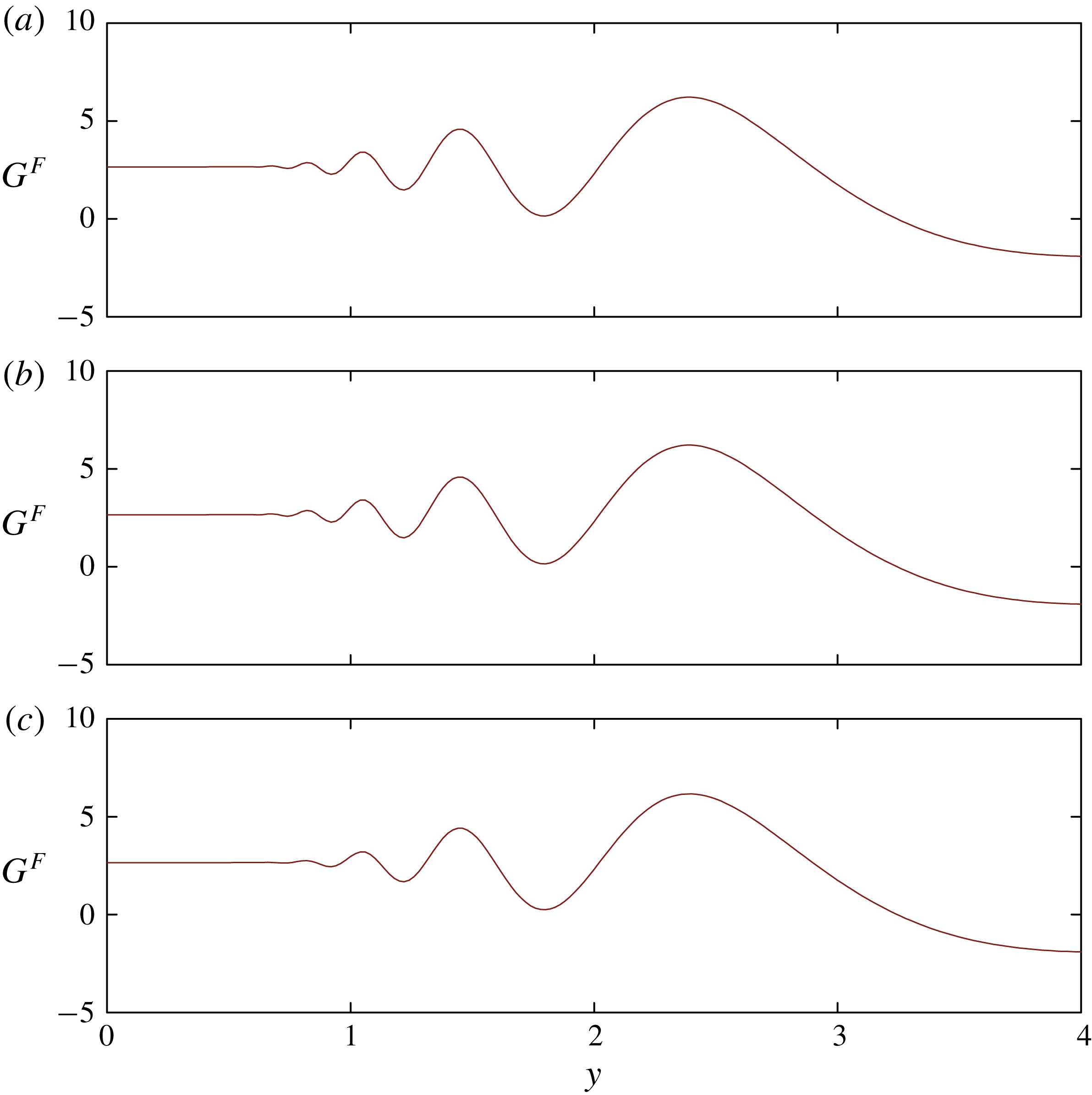
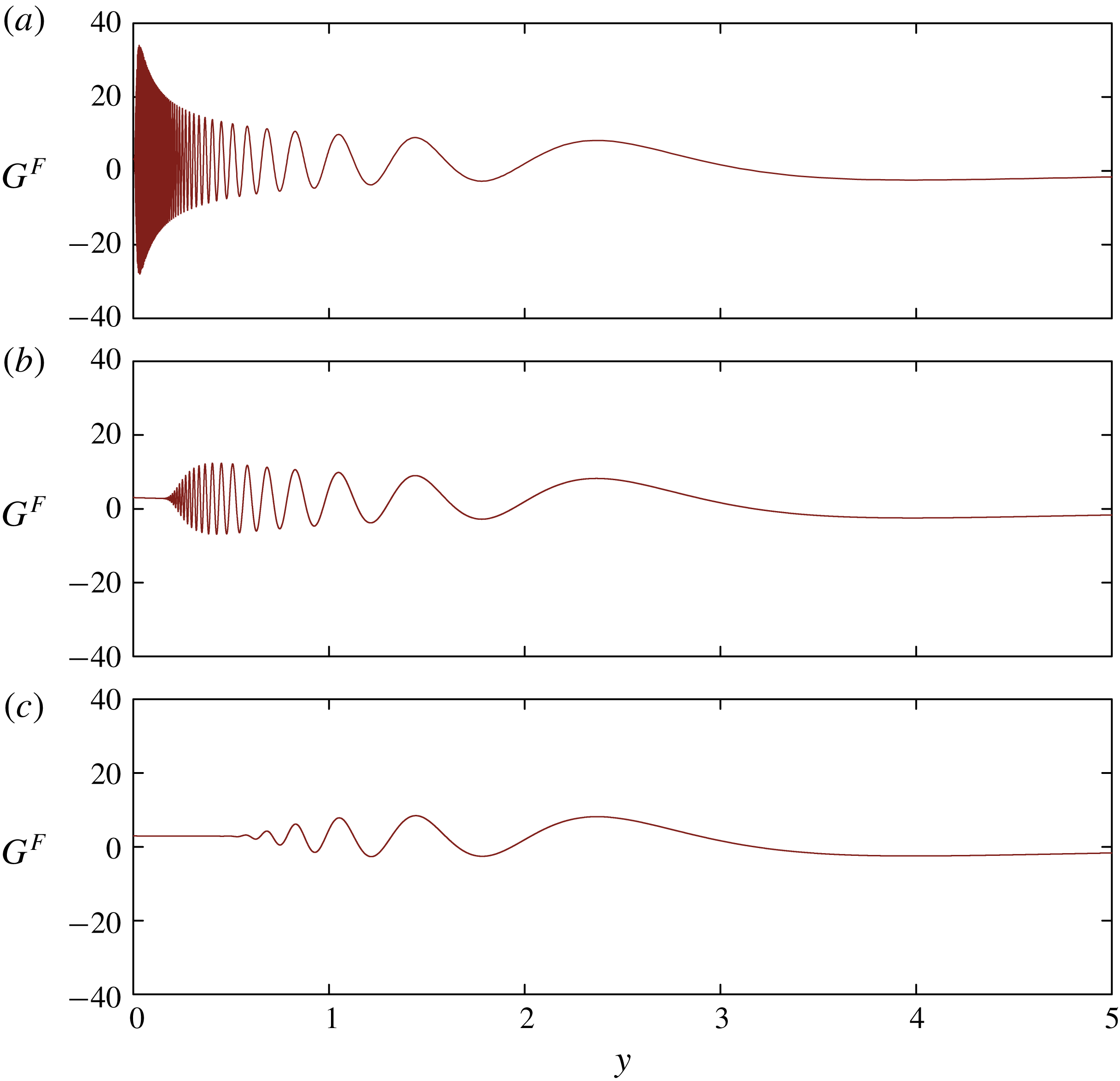
The results based on the numerical evaluation of the viscous-ship-wave Green function are considered. Figures 2 and 3 depict the free-surface term
 $G^{F}$
varying along a transverse cut in the downstream at
 $x=10.0$
generated by a fully submerged source
 $d=0.1$
and a slightly submerged source
 $d=1.0\times 10^{-5}$
with unit strength. The translating speed of the point source is
 $\mathscr{U}=3.132~\text{m}~\text{s}^{-1}$
. Here, both the pure gravity ship-wave Green function and the viscous-ship-wave Green function are displayed. Besides, two different non-dimensional viscosity coefficients
 $\unicode[STIX]{x1D716}=3.2\times 10^{-7}$
and
 $\unicode[STIX]{x1D716}=3.2\times 10^{-5}$
corresponding to the kinematic fluid viscosities
 $\unicode[STIX]{x1D708}=10^{-6}~\text{m}^{2}~\text{s}^{-1}$
and
 $\unicode[STIX]{x1D708}=10^{-4}~\text{m}^{2}~\text{s}^{-1}$
are considered.
The free-surface term
 $G^{F}$
induced by a source with the submergence
 $d=gD/\mathscr{U}^{2}=0.1$
and the translating speed
 $\mathscr{U}=3.132~\text{m}~\text{s}^{-1}$
varying along a transverse cut at
 $x=gX/\mathscr{U}^{2}=10.0$
. (a) Pure gravity ship-wave Green function; (b) viscous-ship-wave Green function with
 $\unicode[STIX]{x1D716}=3.2\times 10^{-7}$
corresponding to
 $\unicode[STIX]{x1D708}=10^{-6}~\text{m}^{2}~\text{s}^{-1}$
; (c) viscous-ship-wave Green function with
 $\unicode[STIX]{x1D716}=3.2\times 10^{-5}$
corresponding to
 $\unicode[STIX]{x1D708}=10^{-4}~\text{m}^{2}~\text{s}^{-1}$
.

The free-surface term
 $G^{F}$
induced by a slightly submerged source at
 $d=gD/\mathscr{U}^{2}=1.0\times 10^{-5}$
and the forward speed
 $\mathscr{U}=3.132~\text{m}~\text{s}^{-1}$
varying along a transverse cut at
 $x=gX/\mathscr{U}^{2}=10.0$
. (a) Pure gravity ship-wave Green function; (b) viscous-ship-wave Green function with
 $\unicode[STIX]{x1D716}=3.2\times 10^{-7}$
corresponding to
 $\unicode[STIX]{x1D708}=10^{-6}~\text{m}^{2}~\text{s}^{-1}$
; (c) viscous-ship-wave Green function with
 $\unicode[STIX]{x1D716}=3.2\times 10^{-5}$
corresponding to
 $\unicode[STIX]{x1D708}=10^{-4}~\text{m}^{2}~\text{s}^{-1}$
.

When the singularity is fully submerged
 $d=0.1$
, as shown in figure 2, viscous effects do not make a difference because there is no obvious difference between the three panels. As for a slightly submerged source
 $d=1.0\times 10^{-5}$
, as exhibited in figure 3, the difference is evident. In the top panel, in which viscous effects are ignored, the free-surface term
 $G^{F}$
is strongly oscillatory, and the wave height near the track
 $y=0$
is very large. When only the molecular viscosity
 $\unicode[STIX]{x1D716}=3.2\times 10^{-7}$
is accounted for in the middle panel, waves are greatly damped, but rapid oscillations still exist. When the non-dimensional viscosity coefficient is taken to be
 $\unicode[STIX]{x1D716}=3.2\times 10^{-5}$
in the bottom panel, waves become very smooth and highly oscillatory behaviours are severely damped due to viscous effects. It is noted that viscous effects only attenuate the short waves near the track associated with large wavenumbers. In the region with a relatively large azimuthal angle where short waves do not appear, waves are merely affected by viscous effects.
6.2 Non-uniform asymptotic approximations
Then, we consider the asymptotic approximations to the wave component
 $G^{W}$
due to Kelvin, Havelock and Peters as presented in § 4. For a flow-field point located inside (
 $|\unicode[STIX]{x1D6FE}|<\unicode[STIX]{x1D6FE}_{0}$
), at (
 $|\unicode[STIX]{x1D6FE}|=\unicode[STIX]{x1D6FE}_{0}$
) and outside (
 $|\unicode[STIX]{x1D6FE}|>\unicode[STIX]{x1D6FE}_{0}$
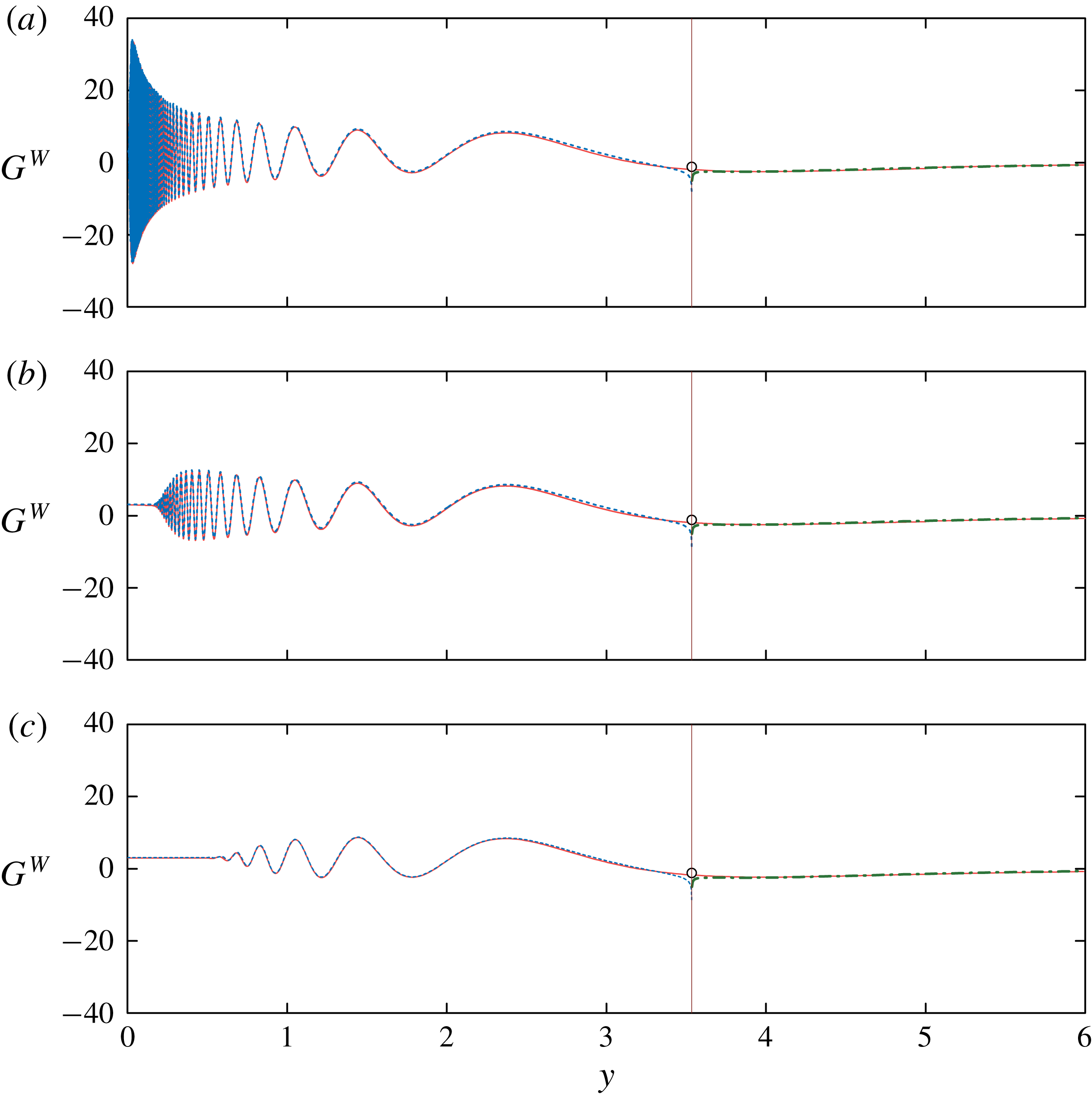
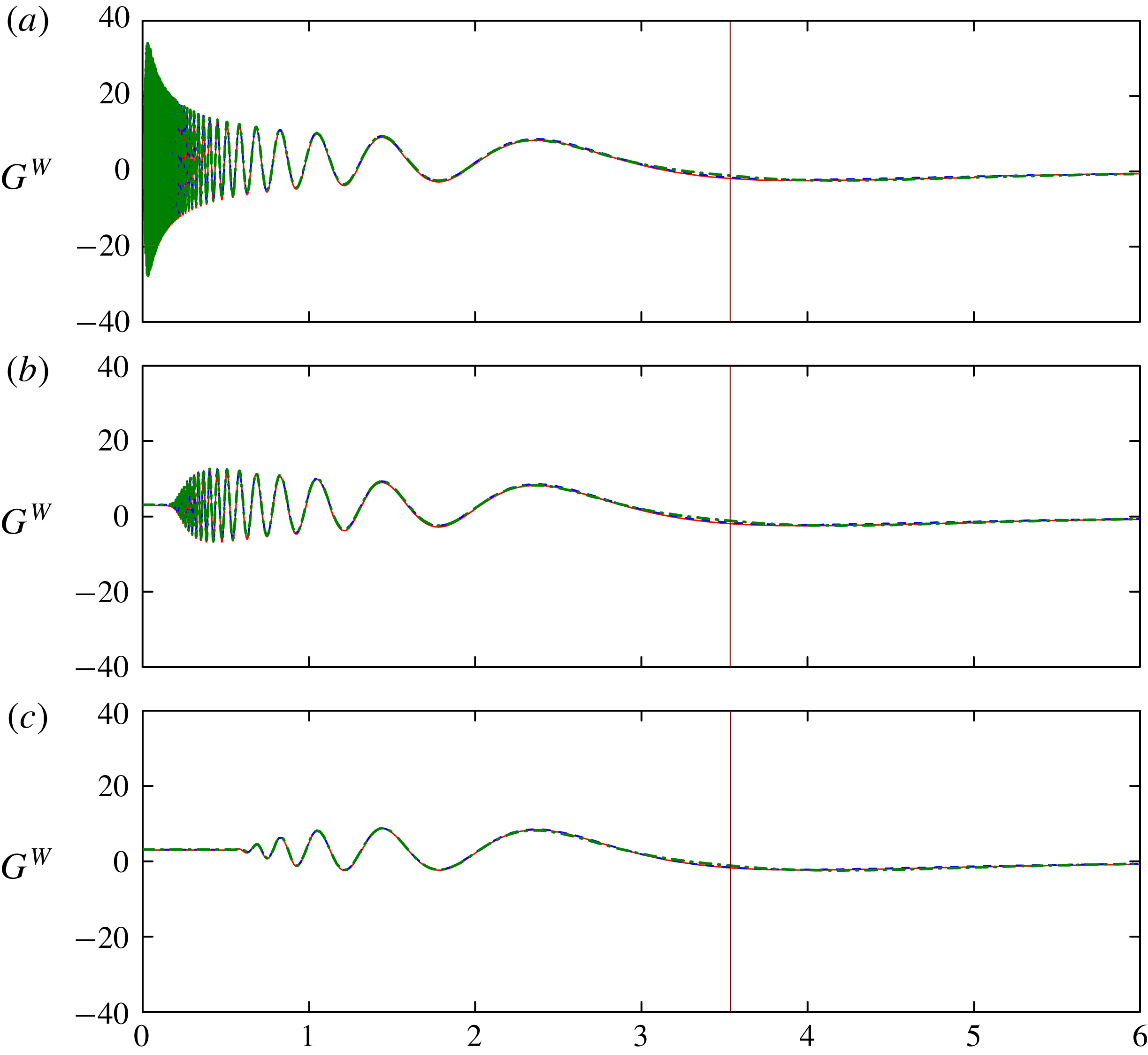
) the Kelvin wedge, expressions (4.11), (4.22) and (4.25) are applied, respectively. Figure 4 shows the comparison between the numerical evaluation and three asymptotic approximations for a slightly submerged source with the submergence
 $d=1.0\times 10^{-5}$
and translating speed
 $\mathscr{U}=3.132~\text{m}~\text{s}^{-1}$
considered in figure 3. Here, the numerical results are represented by solid lines, while the asymptotic approximations due to Kelvin, Havelock and Peters are plotted by dashed lines, hollow symbols and dash–dotted lines, respectively. The Kelvin’s and Peters’ expressions approximate the wave component
 $G^{W}$
well when the azimuthal angle
 $\unicode[STIX]{x1D6FE}$
deviates from the cusp angle
 $\unicode[STIX]{x1D6FE}_{0}$
, and highly oscillatory behaviours of the pure gravity ship-wave Green function are well reflected by the Kelvin’s approximation. At the cusp line, the approximations due to Kelvin and Peters are singular, whereas Havelock’s approximation is well finite and agrees well with the numerical evaluation.
The wave component
 $G^{W}$
induced by a slightly submerged source with the translating speed
 $\mathscr{U}=3.132~\text{m}~\text{s}^{-1}$
at
 $d=1.0\times 10^{-5}$
varying along a transverse cut at
 $x=10.0$
. The comparison is made between the numerical evaluation by solid lines (——) and the asymptotic approximations due to Kelvin, Havelock and Peters represented by the dashed lines (– – – –), hollow scatters (○) and dash–dotted lines (– ⋅ – ⋅ –), respectively. (a) Pure gravity ship-wave Green function; (b) viscous-ship-wave Green function with
 $\unicode[STIX]{x1D716}=3.2\times 10^{-7}$
; (c) viscous-ship-wave Green function with
 $\unicode[STIX]{x1D716}=3.2\times 10^{-5}$
. The vertical line
 $y\approx 3.5$
corresponds to the cusp of Kelvin wedge.

6.3 Uniform approximations
Uniform approximations based on the CFU approximation and KHP approximation elucidated in § 5 are considered here. Figure 5 exhibits the wave component
 $G^{W}$
induced by a slightly submerged translating source with the submergence
 $d=1.0\times 10^{-5}$
and translating speed
 $\mathscr{U}=3.132~\text{m}~\text{s}^{-1}$
considered in figure 3. Results obtained from the CFU approximation and the KHP approximation are compared with the direct numerical evaluation. Generally, these three groups of results are in close agreement. Nevertheless, a slight difference is witnessed between the KHP approximation and the two others near the cusp line
 $\unicode[STIX]{x1D6FE}=\unicode[STIX]{x1D6FE}_{0}$
. It has already been pointed out by Wu et al. (Reference Wu, He, Zhu and Noblesse2018) that the KHP approximation is not as accurate as the CFU approximation in proximity to cusps. The KHP approximation is consistent with Havelock’s expression at the cusp line. It is noted that the reminder of Havelock’s approximation (4.22) is of the order of
 $O(R^{-2/3})$
. However, the error of the CFU approximation is of the order of
 $O(R^{-4/3})$
. Therefore, the CFU approximation is more accurate, but the accuracy of the KHP approximation can be improved by introducing high-order asymptotic expressions. The refined KHP approximation has been recently studied by Liang et al. (Reference Liang, Wu, He and Noblesse2020).
The wave component
 $G^{W}$
induced by a slightly submerged source with the translating speed
 $\mathscr{U}=3.132~\text{m}~\text{s}^{-1}$
at
 $d=gD/\mathscr{U}^{2}=1.0\times 10^{-5}$
varying along a transverse cut at
 $x=gX/\mathscr{U}^{2}=10.0$
. The comparison is made between the numerical evaluation by solid lines (——) and the uniform asymptotic approximations based on the CFU approximation by dashed lines (– – – –) and KHP approximation by dash-dotted lines (– ⋅ – ⋅ –). (a) Pure gravity ship-wave Green function; (b) viscous-ship-wave Green function with
 $\unicode[STIX]{x1D716}=3.2\times 10^{-7}$
; (c) viscous-ship-wave Green function with
 $\unicode[STIX]{x1D716}=3.2\times 10^{-5}$
. The vertical line
 $y\approx 3.5$
corresponds to the cusp of Kelvin wedge.

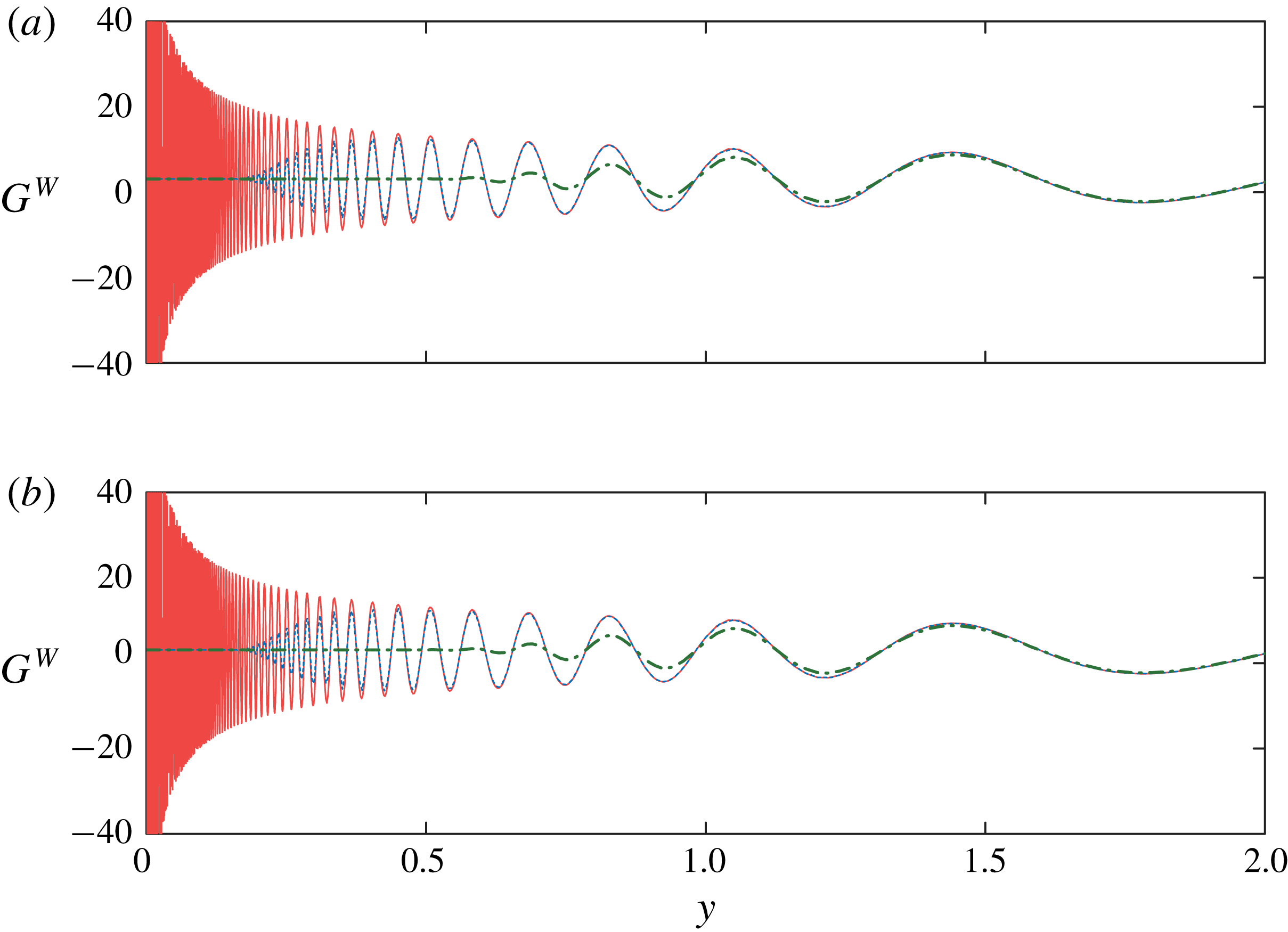
Figure 6 depicts the wave component
 $G^{W}$
induced by a source exactly located at the free surface
 $d=0$
with the translating speed
 $\mathscr{U}=3.132~\text{m}~\text{s}^{-1}$
varying along a transverse cut at
 $x=10.0$
. Besides the pure gravity ship-wave Green function, the viscous-ship-wave Green functions with viscosity coefficients
 $\unicode[STIX]{x1D716}=3.2\times 10^{-7}$
and
 $\unicode[STIX]{x1D716}=3.2\times 10^{-5}$
are exhibited. Results determined by the CFU approximation and KHP approximation are displayed in the top and bottom panels, respectively. It provides strong evidence that singular and highly oscillatory behaviours in the pure gravity ship-wave Green function are eliminated and damped by including viscous effects. Furthermore, steep short waves still exist if only molecular viscosity is accounted for, and can be largely removed via taking a proper viscosity coefficient, i.e. 100 times the molecular viscosity coefficient as suggested by Dias et al. (Reference Dias, Dyachenko and Zakharov2008) and Horsley & Forbes (Reference Horsley and Forbes2013).
The wave component
 $G^{W}$
induced by a source exactly at the free surface
 $d=gD/\mathscr{U}^{2}=0$
with the translating speed
 $\mathscr{U}=3.132~\text{m}~\text{s}^{-1}$
varying along a transverse cut at
 $x=gX/\mathscr{U}^{2}=10.0$
. Three groups of results are displayed including the pure gravity ship-wave Green function by solid lines (——), viscous-ship-wave Green functions with
 $\unicode[STIX]{x1D716}=3.2\times 10^{-7}$
(
 $\unicode[STIX]{x1D708}=10^{-6}~\text{m}^{2}~\text{s}^{-1}$
) plotted by dashed lines (– – – –) and
 $\unicode[STIX]{x1D716}=3.2\times 10^{-5}$
(
 $\unicode[STIX]{x1D708}=10^{-4}~\text{m}^{2}~\text{s}^{-1}$
) by dash-dotted lines (– ⋅ – ⋅ –). (a) CFU approximation; (b) KHP approximation.

Figure 7 shows the plan view of the free-surface pattern generated by a steadily translating source with the submergence
 $d=5.0\times 10^{-2}$
and travelling speed
 $\mathscr{U}=3.132~\text{m}~\text{s}^{-1}$
in a rectangular region
 $10\leqslant x\leqslant 20$
,
 $0\leqslant y\leqslant 8$
. Results obtained from the numerical evaluation, the CFU approximation and KHP approximation are placed in the top row, centre row and bottom row, respectively. The pure gravity ship waves as well as viscous ship waves with the viscosity coefficients
 $\unicode[STIX]{x1D716}=3.2\times 10^{-7}$
and
 $\unicode[STIX]{x1D716}=3.2\times 10^{-5}$
are shown in the left column, middle column and right column, respectively. Discrepancies of wave patterns determined via three methods are indistinguishable. When viscous effects are ignored or only the molecular viscosity is accounted for, short waves are present inside the Kelvin wedge. In the right column in which the kinematic fluid viscosity coefficient is
 $\unicode[STIX]{x1D716}=3.2\times 10^{-5}$
, short waves die out.
Plan view of the free-surface elevation generated by a steadily translating source with the submergence
 $d=gD/\mathscr{U}^{2}=5.0\times 10^{-2}$
and the travelling speed
 $\mathscr{U}=3.132~\text{m}~\text{s}^{-1}$
. Numerical evaluations are shown in (a–c), results determined by the CFU approximation in (d–f) and results by the KHP approximation in (g–i). Pure gravity ship waves as well as viscous ship waves with viscosity coefficients
 $\unicode[STIX]{x1D716}=3.2\times 10^{-7}$
and
 $\unicode[STIX]{x1D716}=3.2\times 10^{-5}$
corresponding to
 $\unicode[STIX]{x1D708}=10^{-6}~\text{m}^{2}~\text{s}^{-1}$
and
 $\unicode[STIX]{x1D708}=10^{-4}~\text{m}^{2}~\text{s}^{-1}$
, respectively, are placed from left to right. The white dashed line corresponds to the cusp of the Kelvin wedge.

7 Apparent wake angle of waves by a point source
Inspired by observations by Rabaud & Moisy (Reference Rabaud and Moisy2013), the investigation into the apparent wave angle of ship waves has been extensively carried out by considering the bow-stern interference effect (Noblesse et al. Reference Noblesse, He, Zhu, Hong, Zhang, Zhu and Yang2014) and a pressure patch with a smooth distribution (Benzaquen, Darmon & Raphaël Reference Benzaquen, Darmon and Raphaël2014; Darmon, Benzaquen & Raphaël Reference Darmon, Benzaquen and Raphaël2014; Miao & Liu Reference Miao and Liu2015). Besides, as pointed out by Dias (Reference Dias2014), it is important to focus on the amplitude. The subsequent study by Pethiyagoda et al. (Reference Pethiyagoda, McCue and Moroney2014a ) demonstrates that even a point source can generate a wake with a smaller apparent angle than the Kelvin angle. Here, the apparent angle of waves associated with the viscous-ship-wave Green function is considered.
7.1 Decomposition of transverse and divergent waves
The uniform KHP approximation enables us to determine the individual contributions of transverse waves and divergent waves. Figure 8 shows the free-surface elevations induced by a translating source with the submergence
 $d=0.01$
and the translating speed
 $\mathscr{U}=3.132~\text{m}~\text{s}^{-1}$
varying with the ratio between the azimuthal angle and the Kelvin angle
 $\unicode[STIX]{x1D6FE}/\unicode[STIX]{x1D6FE}_{0}$
at a constant radius
 $R=10$
, and where the transverse waves and divergent waves are represented by solid lines and dashed lines, respectively. The envelope of divergent waves is also exhibited and is plotted by dash-dotted lines. In this case, the transverse waves with a small amplitude are mildly varying with the angle, but the divergent waves are oscillatory with an amplitude much higher than that of the transverse waves. Therefore, the divergent waves dominate the wave pattern at small
 $d$
, corresponding to a small submergence or a high travelling speed. In addition, viscous effects hardly affect the transverse waves, but attenuate the amplitude of the divergent waves near the track. Furthermore, there is a narrow region near the track where the amplitude of divergent waves is almost zero when the source is submerged. The middle and bottom panels show that viscous effects make the region wider.
Decomposition of transverse and divergent waves inside the Kelvin wedge. The transverse waves are represented by solid lines (——), divergent waves by dashed lines (– – – –) and the envelope of divergent waves by dash-dotted lines (– ⋅ – ⋅ –). (a) Pure gravity ship waves; (b) viscous ship waves with
 $\unicode[STIX]{x1D716}=3.2\times 10^{-7}$
; (c) viscous ship waves with
 $\unicode[STIX]{x1D716}=3.2\times 10^{-5}$
.

7.2 Apparent wake angle
In order to study the apparent angle of free-surface waves generated by a translating source, the maximum of the envelope of divergent waves is considered. According to § 4.1, the envelope of divergent waves induced by a point source is
 $$\begin{eqnarray}E=\frac{1}{\unicode[STIX]{x03C0}}\sqrt{1+\unicode[STIX]{x1D705}_{+}^{2}}\exp \left[-(1+\unicode[STIX]{x1D705}_{+}^{2})d-4\unicode[STIX]{x1D716}x\frac{(\unicode[STIX]{x1D705}_{+}^{2}+1)^{3}}{2\unicode[STIX]{x1D705}_{+}^{2}+1}\right]\sqrt{\frac{2\unicode[STIX]{x03C0}}{R|\unicode[STIX]{x1D713}_{+}^{\prime \prime }|}},\end{eqnarray}$$
where
 $\unicode[STIX]{x1D705}_{+}$
and
 $\unicode[STIX]{x1D713}_{+}^{\prime \prime }$
are given by
 $$\begin{eqnarray}\unicode[STIX]{x1D705}_{+}\approx \frac{1}{2\unicode[STIX]{x1D6FE}}-\frac{7}{6}\unicode[STIX]{x1D6FE}+O(\unicode[STIX]{x1D6FE}^{3})\quad \text{and}\quad \unicode[STIX]{x1D713}_{+}^{\prime \prime }\approx -2\unicode[STIX]{x1D6FE}+\frac{25}{3}\unicode[STIX]{x1D6FE}^{3}+O(\unicode[STIX]{x1D6FE}^{5}),\end{eqnarray}$$
based on the small azimuthal angle approximation. Following Darmon et al. (Reference Darmon, Benzaquen and Raphaël2014), Pethiyagoda et al. (Reference Pethiyagoda, McCue and Moroney2014a ), Miao & Liu (Reference Miao and Liu2015), the envelope of the divergent waves is expanded as
 $$\begin{eqnarray}\displaystyle E & {\approx} & \displaystyle \frac{1}{\sqrt{\unicode[STIX]{x03C0}R}}\left(\frac{1}{2}\unicode[STIX]{x1D6FE}^{-3/2}+\frac{7}{8}\unicode[STIX]{x1D6FE}^{1/2}+\cdots \right)\nonumber\\ \displaystyle & & \displaystyle \times \exp \left[-\frac{\unicode[STIX]{x1D716}x}{8}\unicode[STIX]{x1D6FE}^{-4}-\left(\frac{\unicode[STIX]{x1D716}x}{12}+\frac{d}{4}\right)\unicode[STIX]{x1D6FE}^{-2}+\frac{107}{180}\unicode[STIX]{x1D716}x+\frac{d}{6}+\cdots \right].\end{eqnarray}$$
By differentiating
 $E$
with respect to
 $\unicode[STIX]{x1D6FE}$
and setting it to zero
 $\unicode[STIX]{x2202}E/\unicode[STIX]{x2202}\unicode[STIX]{x1D6FE}=0$
, we can obtain the maximum wake angle subject to
 $$\begin{eqnarray}\frac{\unicode[STIX]{x1D716}x}{2}\unicode[STIX]{x1D6FE}^{-4}+\left(\frac{25}{24}\unicode[STIX]{x1D716}x+\frac{d}{2}\right)\unicode[STIX]{x1D6FE}^{-2}-\frac{3}{2}=0,\end{eqnarray}$$
resulting in the apparent wake angle in a simple expression:
 $$\begin{eqnarray}\unicode[STIX]{x1D6FE}_{app}\approx \frac{1}{\sqrt{3}}\sqrt{d}+\frac{\sqrt{3}}{2}\frac{\unicode[STIX]{x1D716}x}{d^{3/2}}=\frac{\sqrt{gD}}{\sqrt{3}\mathscr{U}}+\frac{\sqrt{3}}{2}\frac{\unicode[STIX]{x1D708}X\sqrt{g}}{D^{3/2}\mathscr{U}^{2}}.\end{eqnarray}$$
When viscous effects are disregarded, expression (7.5) is consistent with the one given by Pethiyagoda et al. (Reference Pethiyagoda, McCue and Moroney2014a
). Nevertheless, the apparent wake angle under the influence of viscous effects is dependent on the distance along the track from the point source, and it is associated with both
 $\mathscr{U}^{-1}$
and
 $\mathscr{U}^{-2}$
. Furthermore, viscous effects play an increasingly important role with increasing distance. Figures 9 and 10 show the apparent wake angle induced by a translating source as a function of the submergence Froude number
 $F_{d}=\mathscr{U}/\sqrt{gD}$
at a fixed immersion depth
 $D=0.01$
m and at a constant speed
 $\mathscr{U}=31.3~\text{m}~\text{s}^{-1}$
. The asymptotic expression is exhibited by solid symbols, and the direct measurements are by solid lines. At a high submergence Froude number, viscous effects make a difference, and the apparent wake angle associated with viscous ship waves is larger than the pure gravity counterpart.
Apparent wake angle induced by a source with the submergence
 $D=0.01$
m as a function of the submergence Froude number
 $F_{d}=\mathscr{U}/\sqrt{gD}$
. The direct measurements are represented by solid lines, and the results determined by the asymptotic approximation (7.5) by solid symbols. The dashed line corresponds to the Kelvin angle.

Apparent wake angle induced by a source at a constant speed
 $\mathscr{U}=31.3~\text{m}~\text{s}^{-1}$
as a function of the submergence Froude number
 $F_{d}=\mathscr{U}/\sqrt{gD}$
. The direct measurements are represented by solid lines, and the results determined by the asymptotic approximation (7.5) by solid symbols. The dashed line corresponds to the Kelvin angle.

8 Concluding remarks
This paper presents a systematic study of the viscous-ship-wave Green function within the framework of weakly damped free-surface flows (Dias et al. Reference Dias, Dyachenko and Zakharov2008), and both numerical and analytical investigations are conducted. An explicit expression of the Green function in the form of a double Fourier integral is firstly formulated. Then, an efficient and accurate evaluation method is described by decomposing the free-surface term into a non-oscillatory local-flow component and a wave component dominant in the far field using Cauchy’s residue theorem. To delve deeper into the flow physics of the viscous-ship-wave Green function, both non-uniform (Kelvin Reference Kelvin1887; Havelock Reference Havelock1908; Peters Reference Peters1949) and uniform asymptotic approximations (Chester et al. Reference Chester, Friedman and Ursell1957; Wu et al. Reference Wu, He, Zhu and Noblesse2018) to far-field waves are made. Through this study, the following conclusions can be drawn:
(i) Viscous effects only contribute to the imaginary part of the dispersion function. Hence, they do not change the profile of the wave pattern, but will attenuate the amplitude of waves. The waves near the track associated with high wavenumbers are more susceptible to be influenced by viscous effects, and thus divergent waves are more severely damped. When the source is immersed, there is a narrow region near the cusp where the amplitude of divergent waves is almost zero. Viscous effects render this region wider.
(ii) Under the influence of viscous effects, the singular behaviour, which occurs in the pure gravity ship-wave Green function when both source and flow-field points are located on the free surface and the flow-field point approaches the track of the source point, is eliminated. If only the molecular viscosity
 $\unicode[STIX]{x1D708}=1.0\times 10^{-6}~\text{m}^{2}~\text{s}^{-1}$
is taken, steep short waves are still present. As suggested by Dias et al. (Reference Dias, Dyachenko and Zakharov2008) and Horsley & Forbes (Reference Horsley and Forbes2013), we take 100 times the molecular viscosity, i.e.
 $\unicode[STIX]{x1D708}=1.0\times 10^{-4}~\text{m}^{2}~\text{s}^{-1}$
, and short waves to a large extent die out.
(iii) The KHP approximation provides a formal decomposition of transverse and divergent waves. At a high speed, the divergent waves dominate the wave pattern. The apparent wake angle of free-surface waves generated by a translating source is dependent on viscous effects, and the apparent wake angle of viscous ship waves is larger than for pure gravity ship waves. Under the influence of viscous effects, the apparent wake angle is associated with both
 $\mathscr{U}^{-1}$
and
 $\mathscr{U}^{-2}$
.
This study not only gives an insight into the influence of viscous effects on the fundamental solution to ship waves, but also provides a practical solution to removing non-physically singular and highly oscillatory behaviours embedded in the fundamental solution to ship waves.
Acknowledgements
The authors are grateful to Professor Y.-Z. Dai at Harbin Institute of Technology (Weihai, China) for kindly providing his unpublished notes to help authors to understand the CFU approximation. Constructive comments from three referees are highly appreciated. The second author has been partially supported by the National Natural Science Foundation of China (no. 51779054).
Appendix A. Free-surface boundary condition with viscous effects
This appendix reformulates the free-surface boundary condition accounting for viscous effects. It is assumed that the fluid is incompressible. Viscous effects are accounted for, but the surface tension effect is disregarded. The flow is governed by the continuity equation and the conservation of fluid momentum
 $$\begin{eqnarray}\displaystyle & \unicode[STIX]{x1D735}\boldsymbol{\cdot }\boldsymbol{U}=0, & \displaystyle\end{eqnarray}$$
 $$\begin{eqnarray}\displaystyle & \displaystyle \frac{\unicode[STIX]{x2202}\boldsymbol{U}}{\unicode[STIX]{x2202}T}=-\frac{1}{\unicode[STIX]{x1D70C}}\unicode[STIX]{x1D735}P+\unicode[STIX]{x1D735}(-gZ)+\unicode[STIX]{x1D708}\unicode[STIX]{x1D6FB}^{2}\boldsymbol{U}, & \displaystyle\end{eqnarray}$$
 $\boldsymbol{U}=(U,V,W)$
,
 $T$
,
 $\unicode[STIX]{x1D70C}$
,
 $P$
,
 $g$
and
 $\unicode[STIX]{x1D708}$
represent the velocity components, time, fluid density, pressure, gravity acceleration and kinematic viscosity coefficient, respectively. Here, equation (A 1b
) are the linearized Navier–Stokes equations with the advection term omitted.
On the free surface described by
 $Z=\unicode[STIX]{x1D6EF}(X,Y,T)$
, one kinematic boundary condition and two dynamic boundary conditions are satisfied (Dias et al.
Reference Dias, Dyachenko and Zakharov2008)
 $$\begin{eqnarray}\displaystyle & \displaystyle \frac{\unicode[STIX]{x2202}\unicode[STIX]{x1D6EF}}{\unicode[STIX]{x2202}T}=W,\quad \text{on}~Z=0, & \displaystyle\end{eqnarray}$$
 $$\begin{eqnarray}\displaystyle & \displaystyle \unicode[STIX]{x1D70C}\unicode[STIX]{x1D708}\left(\frac{\unicode[STIX]{x2202}U}{\unicode[STIX]{x2202}Z}+\frac{\unicode[STIX]{x2202}W}{\unicode[STIX]{x2202}X}\right)=\unicode[STIX]{x1D70C}\unicode[STIX]{x1D708}\left(\frac{\unicode[STIX]{x2202}V}{\unicode[STIX]{x2202}Z}+\frac{\unicode[STIX]{x2202}W}{\unicode[STIX]{x2202}Y}\right)=0,\quad \text{on}~Z=0, & \displaystyle\end{eqnarray}$$
 $$\begin{eqnarray}\displaystyle & \displaystyle P=P_{a}+2\unicode[STIX]{x1D70C}\unicode[STIX]{x1D708}\frac{\unicode[STIX]{x2202}W}{\unicode[STIX]{x2202}Z},\quad \text{on}~Z=0, & \displaystyle\end{eqnarray}$$
 $P_{a}$
is the atmospheric pressure. In accordance with the Helmholtz decomposition theorem, the velocity vector can be decomposed into curl-free and divergence-free components
 $$\begin{eqnarray}\boldsymbol{U}=\unicode[STIX]{x1D735}\unicode[STIX]{x1D6F9}+\boldsymbol{U}^{T},\end{eqnarray}$$
where the scalar function
 $\unicode[STIX]{x1D6F9}$
denotes the velocity potential in irrotational flow satisfying
 $\unicode[STIX]{x1D6FB}^{2}\unicode[STIX]{x1D6F9}=0$
and
 $\boldsymbol{U}^{T}=(U^{T},V^{T},W^{T})$
represents the rotational flow. Substituting (A 3) into governing equations (A 1) yields
 $$\begin{eqnarray}\displaystyle & \unicode[STIX]{x1D6FB}^{2}\unicode[STIX]{x1D6F9}=\unicode[STIX]{x1D735}\boldsymbol{\cdot }\boldsymbol{U}^{T}=0, & \displaystyle\end{eqnarray}$$
 $$\begin{eqnarray}\displaystyle & \displaystyle \frac{\unicode[STIX]{x2202}(\unicode[STIX]{x1D735}\unicode[STIX]{x1D6F9})}{\unicode[STIX]{x2202}T}+\frac{\unicode[STIX]{x2202}\boldsymbol{U}^{T}}{\unicode[STIX]{x2202}T}=-\frac{1}{\unicode[STIX]{x1D70C}}\unicode[STIX]{x1D735}P+\unicode[STIX]{x1D735}(-gZ)+\unicode[STIX]{x1D708}\unicode[STIX]{x1D6FB}^{2}(\unicode[STIX]{x1D735}\unicode[STIX]{x1D6F9}+\boldsymbol{U}^{T}). & \displaystyle\end{eqnarray}$$
Taking the curl of (A 4b ) gives rise to
 $$\begin{eqnarray}\displaystyle & \displaystyle \frac{\unicode[STIX]{x2202}\unicode[STIX]{x1D6F9}}{\unicode[STIX]{x2202}T}+\frac{P-P_{a}}{\unicode[STIX]{x1D70C}}+gZ=0, & \displaystyle\end{eqnarray}$$
 $$\begin{eqnarray}\displaystyle & \displaystyle \frac{\unicode[STIX]{x2202}\boldsymbol{U}^{T}}{\unicode[STIX]{x2202}T}=\unicode[STIX]{x1D708}\unicode[STIX]{x1D6FB}^{2}\boldsymbol{U}^{T}, & \displaystyle\end{eqnarray}$$
 $$\begin{eqnarray}\displaystyle & \displaystyle \frac{\unicode[STIX]{x2202}\unicode[STIX]{x1D6EF}}{\unicode[STIX]{x2202}T}=\frac{\unicode[STIX]{x2202}\unicode[STIX]{x1D6F9}}{\unicode[STIX]{x2202}Z}+W^{T},\quad \text{on}~Z=0, & \displaystyle\end{eqnarray}$$
 $$\begin{eqnarray}\displaystyle & \displaystyle 2\frac{\unicode[STIX]{x2202}^{2}\unicode[STIX]{x1D6F9}}{\unicode[STIX]{x2202}X\unicode[STIX]{x2202}Z}+\frac{\unicode[STIX]{x2202}U^{T}}{\unicode[STIX]{x2202}Z}+\frac{\unicode[STIX]{x2202}W^{T}}{\unicode[STIX]{x2202}X}=2\frac{\unicode[STIX]{x2202}^{2}\unicode[STIX]{x1D6F9}}{\unicode[STIX]{x2202}Y\unicode[STIX]{x2202}Z}+\frac{\unicode[STIX]{x2202}V^{T}}{\unicode[STIX]{x2202}Z}+\frac{\unicode[STIX]{x2202}W^{T}}{\unicode[STIX]{x2202}Y}=0,\quad \text{on}~Z=0, & \displaystyle\end{eqnarray}$$
 $$\begin{eqnarray}\displaystyle & \displaystyle \frac{\unicode[STIX]{x2202}\unicode[STIX]{x1D6F9}}{\unicode[STIX]{x2202}T}+g\unicode[STIX]{x1D6EF}+2\unicode[STIX]{x1D708}\left(\frac{\unicode[STIX]{x2202}^{2}\unicode[STIX]{x1D6F9}}{\unicode[STIX]{x2202}Z^{2}}+\frac{\unicode[STIX]{x2202}W^{T}}{\unicode[STIX]{x2202}Z}\right)=0,\quad \text{on}~Z=0. & \displaystyle\end{eqnarray}$$
Differentiating (A 6c
) with respect to
 $T$
and combining with (A 6a
), we have
 $$\begin{eqnarray}\frac{\unicode[STIX]{x2202}^{2}\unicode[STIX]{x1D6F9}}{\unicode[STIX]{x2202}T^{2}}+g\frac{\unicode[STIX]{x2202}\unicode[STIX]{x1D6F9}}{\unicode[STIX]{x2202}Z}+gW^{T}+2\unicode[STIX]{x1D708}\frac{\unicode[STIX]{x2202}}{\unicode[STIX]{x2202}T}\left(\frac{\unicode[STIX]{x2202}^{2}\unicode[STIX]{x1D6F9}}{\unicode[STIX]{x2202}Z^{2}}+\frac{\unicode[STIX]{x2202}W^{T}}{\unicode[STIX]{x2202}Z}\right)=0,\quad \text{on}~Z=0.\end{eqnarray}$$
According to the derivation presented in appendix B, we have the relation between
 $\unicode[STIX]{x1D6EF}$
and
 $W^{T}$
 $$\begin{eqnarray}W^{T}=2\unicode[STIX]{x1D708}\left(\frac{\unicode[STIX]{x2202}^{2}\unicode[STIX]{x1D6EF}}{\unicode[STIX]{x2202}X^{2}}+\frac{\unicode[STIX]{x2202}^{2}\unicode[STIX]{x1D6EF}}{\unicode[STIX]{x2202}Y^{2}}\right),\quad \text{on}~Z=0.\end{eqnarray}$$
Substituting (A 6c ) into (A 8), we have
 $$\begin{eqnarray}W^{T}\approx 2\unicode[STIX]{x1D708}\left(\frac{\unicode[STIX]{x2202}^{2}}{\unicode[STIX]{x2202}X^{2}}+\frac{\unicode[STIX]{x2202}^{2}}{\unicode[STIX]{x2202}Y^{2}}\right)\left[-\frac{1}{g}\frac{\unicode[STIX]{x2202}\unicode[STIX]{x1D6F9}}{\unicode[STIX]{x2202}T}-\frac{2\unicode[STIX]{x1D708}}{g}\left(\frac{\unicode[STIX]{x2202}^{2}\unicode[STIX]{x1D6F9}}{\unicode[STIX]{x2202}Z^{2}}+\frac{\unicode[STIX]{x2202}W^{T}}{\unicode[STIX]{x2202}Z}\right)\right]\approx \frac{2\unicode[STIX]{x1D708}}{g}\frac{\unicode[STIX]{x2202}^{3}\unicode[STIX]{x1D6F9}}{\unicode[STIX]{x2202}T\unicode[STIX]{x2202}Z^{2}},\quad \text{on}~Z=0,\end{eqnarray}$$
where the quadratic terms associated with the viscosity are omitted. By inserting (A 9) into (A 7), we can obtain a new linear free-surface condition accounting for viscous effects
 $$\begin{eqnarray}\frac{\unicode[STIX]{x2202}^{2}\unicode[STIX]{x1D6F9}}{\unicode[STIX]{x2202}T^{2}}+g\frac{\unicode[STIX]{x2202}\unicode[STIX]{x1D6F9}}{\unicode[STIX]{x2202}Z}+4\unicode[STIX]{x1D708}\frac{\unicode[STIX]{x2202}^{3}\unicode[STIX]{x1D6F9}}{\unicode[STIX]{x2202}T\unicode[STIX]{x2202}Z^{2}}=0,\quad \text{on}~Z=0,\end{eqnarray}$$
where the Laplace equation
 $\unicode[STIX]{x1D6FB}^{2}\unicode[STIX]{x1D6F9}=0$
is applied. In a reference of frame steadily translating with a body, the potential is written as
 $\unicode[STIX]{x1D6F9}=\mathscr{U}X+\unicode[STIX]{x1D6F7}$
, and then linear free-surface boundary condition becomes
 $$\begin{eqnarray}\mathscr{U}^{2}\frac{\unicode[STIX]{x2202}^{2}\unicode[STIX]{x1D6F7}}{\unicode[STIX]{x2202}X^{2}}+g\frac{\unicode[STIX]{x2202}\unicode[STIX]{x1D6F7}}{\unicode[STIX]{x2202}Z}+4\unicode[STIX]{x1D708}\mathscr{U}\frac{\unicode[STIX]{x2202}^{3}\unicode[STIX]{x1D6F7}}{\unicode[STIX]{x2202}X\unicode[STIX]{x2202}Z^{2}}=0,\quad \text{on}~Z=0.\end{eqnarray}$$
Appendix B. Proof of (A 8)
In Dutykh & Dias (Reference Dutykh and Dias2007), formulation (A 8) is obtained by means of the joint Laplace–Fourier transform. In this appendix, we derive it in a different way via differentiating the free-surface boundary conditions. From the continuity equation given by (A 4a ), we have
 $$\begin{eqnarray}\frac{\unicode[STIX]{x2202}U^{T}}{\unicode[STIX]{x2202}X}+\frac{\unicode[STIX]{x2202}V^{T}}{\unicode[STIX]{x2202}Y}+\frac{\unicode[STIX]{x2202}W^{T}}{\unicode[STIX]{x2202}Z}=0.\end{eqnarray}$$
Differentiating (B 1) with respect to
 $Z$
yields
 $$\begin{eqnarray}\frac{\unicode[STIX]{x2202}^{2}U^{T}}{\unicode[STIX]{x2202}X\unicode[STIX]{x2202}Z}+\frac{\unicode[STIX]{x2202}^{2}V^{T}}{\unicode[STIX]{x2202}Y\unicode[STIX]{x2202}Z}+\frac{\unicode[STIX]{x2202}^{2}W^{T}}{\unicode[STIX]{x2202}Z^{2}}=0.\end{eqnarray}$$
By calculating derivatives of the dynamic free-surface boundary condition (A 2b ), we obtain the following two expressions
 $$\begin{eqnarray}\displaystyle & \displaystyle 2\frac{\unicode[STIX]{x2202}^{3}\unicode[STIX]{x1D6F9}}{\unicode[STIX]{x2202}X^{2}\unicode[STIX]{x2202}Z}+\frac{\unicode[STIX]{x2202}^{2}U^{T}}{\unicode[STIX]{x2202}X\unicode[STIX]{x2202}Z}+\frac{\unicode[STIX]{x2202}^{2}W^{T}}{\unicode[STIX]{x2202}X^{2}}=0, & \displaystyle\end{eqnarray}$$
 $$\begin{eqnarray}\displaystyle & \displaystyle 2\frac{\unicode[STIX]{x2202}^{3}\unicode[STIX]{x1D6F9}}{\unicode[STIX]{x2202}Y^{2}\unicode[STIX]{x2202}Z}+\frac{\unicode[STIX]{x2202}^{2}V^{T}}{\unicode[STIX]{x2202}Y\unicode[STIX]{x2202}Z}+\frac{\unicode[STIX]{x2202}^{2}W^{T}}{\unicode[STIX]{x2202}Y^{2}}=0. & \displaystyle\end{eqnarray}$$
Combining (B 2), (B 3a ) and (B 3b ) yields
 $$\begin{eqnarray}2\left(\frac{\unicode[STIX]{x2202}^{3}\unicode[STIX]{x1D6F9}}{\unicode[STIX]{x2202}X^{2}\unicode[STIX]{x2202}Z}+\frac{\unicode[STIX]{x2202}^{2}W^{T}}{\unicode[STIX]{x2202}X^{2}}+\frac{\unicode[STIX]{x2202}^{3}\unicode[STIX]{x1D6F9}}{\unicode[STIX]{x2202}Y^{2}\unicode[STIX]{x2202}Z}+\frac{\unicode[STIX]{x2202}^{2}W^{T}}{\unicode[STIX]{x2202}Y^{2}}\right)=\frac{\unicode[STIX]{x2202}^{2}W^{T}}{\unicode[STIX]{x2202}X^{2}}+\frac{\unicode[STIX]{x2202}^{2}W^{T}}{\unicode[STIX]{x2202}Y^{2}}+\frac{\unicode[STIX]{x2202}^{2}W^{T}}{\unicode[STIX]{x2202}Z^{2}}.\end{eqnarray}$$
Considering (A 5b ), we have
 $$\begin{eqnarray}\frac{\unicode[STIX]{x2202}W^{T}}{\unicode[STIX]{x2202}T}=\unicode[STIX]{x1D708}\left(\frac{\unicode[STIX]{x2202}^{2}W^{T}}{\unicode[STIX]{x2202}X^{2}}+\frac{\unicode[STIX]{x2202}^{2}W^{T}}{\unicode[STIX]{x2202}Y^{2}}+\frac{\unicode[STIX]{x2202}^{2}W^{T}}{\unicode[STIX]{x2202}Z^{2}}\right).\end{eqnarray}$$
Inserting (B 4) into (B 5) yields
 $$\begin{eqnarray}\frac{\unicode[STIX]{x2202}W^{T}}{\unicode[STIX]{x2202}T}=2\unicode[STIX]{x1D708}\left[\frac{\unicode[STIX]{x2202}^{2}}{\unicode[STIX]{x2202}X^{2}}\left(\frac{\unicode[STIX]{x2202}\unicode[STIX]{x1D6F9}}{\unicode[STIX]{x2202}Z}+W^{T}\right)+\frac{\unicode[STIX]{x2202}^{2}}{\unicode[STIX]{x2202}Y^{2}}\left(\frac{\unicode[STIX]{x2202}\unicode[STIX]{x1D6F9}}{\unicode[STIX]{x2202}Z}+W^{T}\right)\right].\end{eqnarray}$$
Accounting for the linearized kinematic free-surface boundary condition in (A 6a ), we can eventually obtain the expression
 $$\begin{eqnarray}W^{T}=2\unicode[STIX]{x1D708}\left(\frac{\unicode[STIX]{x2202}^{2}\unicode[STIX]{x1D6EF}}{\unicode[STIX]{x2202}X^{2}}+\frac{\unicode[STIX]{x2202}^{2}\unicode[STIX]{x1D6EF}}{\unicode[STIX]{x2202}Y^{2}}\right).\end{eqnarray}$$
Appendix C. Exponential-integral function
Consider an integral in the form of
 $$\begin{eqnarray}{\mathcal{I}}=\int _{{\mathcal{C}}_{S}}\frac{1}{k-K}\text{e}^{k{\mathcal{Z}}}\,\text{d}k,\end{eqnarray}$$
where
 ${\mathcal{C}}_{S}$
denotes the integration path along which the exponent
 $k{\mathcal{Z}}$
is purely real so that the exponential function decays most rapidly, as described in figure 1. By performing the change of variable
 $k=r(1+\text{i}\tan \unicode[STIX]{x1D6EC})$
and
 $u=-r{\mathcal{Z}}(1+\text{i}\tan \unicode[STIX]{x1D6EC})$
, expression (C 1) becomes
 $$\begin{eqnarray}{\mathcal{I}}=\int _{0}^{\infty }\frac{1}{r(1+\text{i}\tan \unicode[STIX]{x1D6EC})-K}(1+\text{i}\tan \unicode[STIX]{x1D6EC})\text{e}^{r(1+\text{i}\tan \unicode[STIX]{x1D6EC}){\mathcal{Z}}}\,\text{d}r=\int _{0}^{\infty }\frac{{\mathcal{Z}}}{u+K{\mathcal{Z}}}\frac{\text{e}^{-u}}{{\mathcal{Z}}}\,\text{d}u.\end{eqnarray}$$
Then, representation (C 2) can be further rewritten as
 $$\begin{eqnarray}{\mathcal{I}}=\int _{0}^{\infty }\frac{\text{e}^{-u}}{u+K{\mathcal{Z}}}\,\text{d}u.\end{eqnarray}$$
The exponential-integral function is defined as follows (Abramowitz & Stegun Reference Abramowitz and Stegun1964):
 $$\begin{eqnarray}E_{1}(w)=\int _{w}^{\infty }\frac{\text{e}^{-t}}{t}\,\text{d}t.\end{eqnarray}$$
As a consequence, the integral given by (C 1) can be expressed as
 $$\begin{eqnarray}{\mathcal{I}}=\text{e}^{K{\mathcal{Z}}}E_{1}(K{\mathcal{Z}}).\end{eqnarray}$$