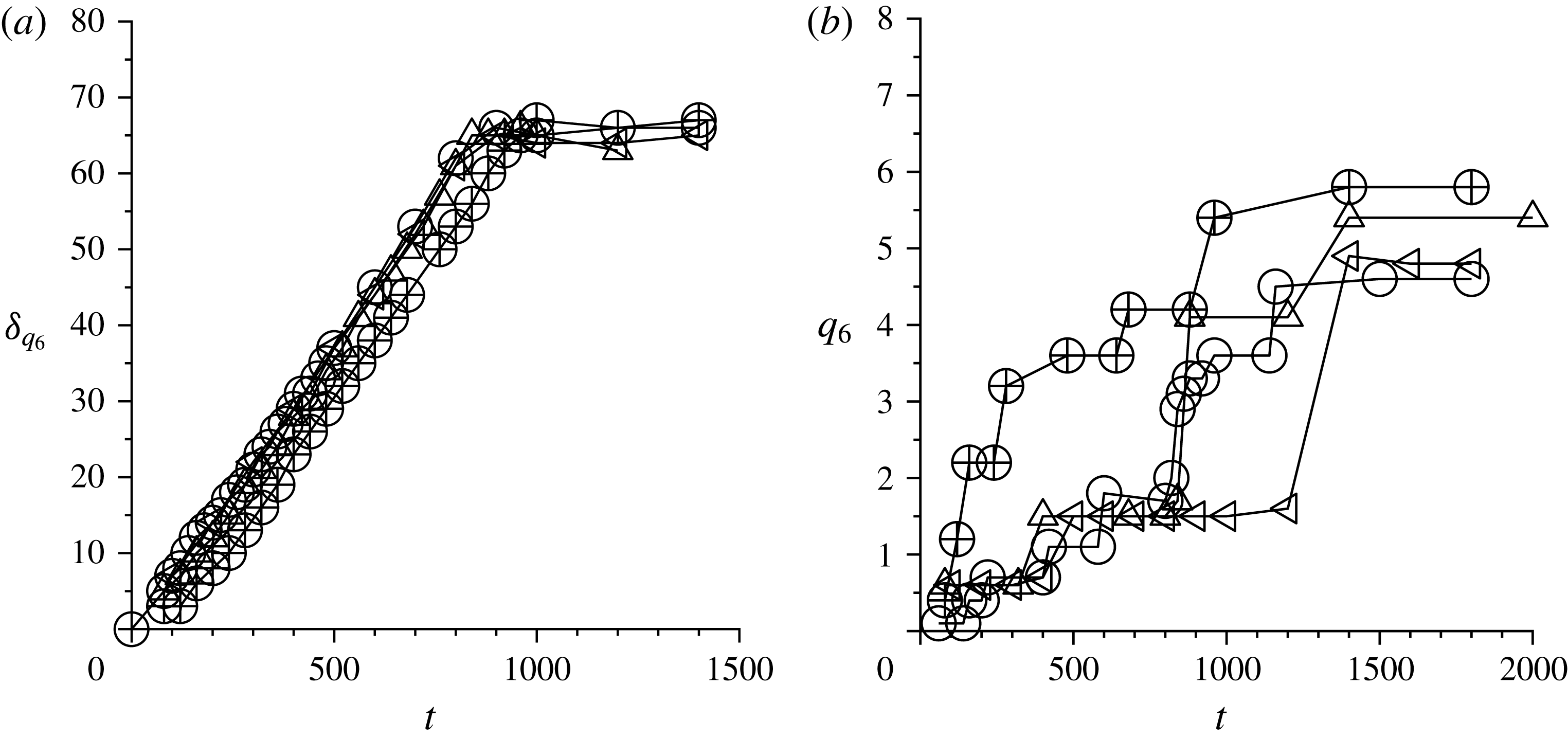
1 Introduction
Apparently simple dense granular flows are known to exhibit unusual features. Recent advances in particle-level simulations have revealed that simple microscopic interaction laws between the particles (Cundall & Strack Reference Cundall and Strack1979; Walton Reference Walton1993; Campbell Reference Campbell2002, Reference Campbell2005) could reproduce many of the complex macroscopic phenomena that are observed in real granular systems, including patterns and solitary waves (Bougie et al.
Reference Bougie, Kreft, Swift and Swinney2005), and convection rolls in vibrated systems (Ramirez, Risso & Cordero Reference Ramirez, Risso and Cordero2000; Sunthar & Kumaran Reference Sunthar and Kumaran2001). For dense granular flows down inclined planes, simulations employing monodisperse hard spherical particles (Silbert et al.
Reference Silbert, Ertas, Grest, Halsey, Levine and Plimpton2001) indicated that a stable flow is observed for a range of angles of inclination from approximately
 $21^{\circ }$
to
 $25^{\circ }$
. Within the flowing layer, it is observed that the volume fraction is independent of the flow depth, in contrast to the compaction expected due to the increased overburden as the flow depth increases. There is a variation in the volume fraction within regions of thickness 3–5 particle diameters at the top and bottom of the flowing layer. The velocity profile is found to satisfy the ‘Bagnold’ profile, which is expected if all components of the stress are proportional to the square of the strain rate. The simulations also appear to capture the intriguing relationships (Pouliquen Reference Pouliquen1999) between the Froude number
 $Fr=(\bar{v}/\sqrt{gh})$
for a flowing layer and
 $h_{stop}$
, the height of the static layer left behind on the inclined plane after cessation of flow. Here,
 $\bar{v}$
is the average velocity,
 $g$
is the acceleration due to gravity and
 $h$
is the height of the flowing layer. Subsequent studies seemed to indicate that the relationship between
 $h_{stop}$
and the Froude number could be better described by scaling laws involving the angle of inclination (Jenkins Reference Jenkins2007), and that the base dissipation has a significant effect on
 $h_{stop}$
(Maheshwari & Kumaran Reference Maheshwari and Kumaran2012). However, the intriguing features of the dense granular flow down an inclined plane have provided an impetus for a large amount of subsequent research.
Phenomenological models have been used to analyse many of the features of the dense granular flow down an inclined plane. Mixing length models (Ertas & Halsey Reference Ertas and Halsey2002) postulate a growing correlation length to model the relation between
 $h_{stop}$
and the Froude number, although evidence for a diverging correlation length in simulations is uncertain (Baran et al.
Reference Baran, Ertas, Halsey, Grest and Lechman2006). Frictional models (MiDi Reference MiDi2004) extend the concept of static yield to derive a shear-rate-dependent criterion for the ratio of the shear and normal stresses. Here, the ratio of shear and normal stresses,
 $\unicode[STIX]{x1D707}=(\unicode[STIX]{x1D70E}/p)$
, is expressed in terms of the inertia number
 $I=(\dot{\unicode[STIX]{x1D6FE}}d/\sqrt{p/\unicode[STIX]{x1D70C}})$
, where
 $\unicode[STIX]{x1D70E}$
and
 $p$
are the shear stress and pressure,
 $\dot{\unicode[STIX]{x1D6FE}}$
is the strain rate and
 $d$
is the particle diameter. A universal form has been proposed for the relation between
 $\unicode[STIX]{x1D707}$
and
 $I$
(MiDi Reference MiDi2004), and the relationship has been extended to three-dimensional flows with the assumption that the stress and rate-of-deformation tensor are collinear (Jop, Forterre & Pouliquen Reference Jop, Forterre and Pouliquen2006). However, the
 $\unicode[STIX]{x1D707}(I)$
relationship provides only one equation between three quantities, the pressure, the shear stress and the rate of deformation. While this may sufficient in flows where the pressure is fixed, it is not sufficient for general three-dimensional flows, and one other relationship is required. This is usually in the form of an incompressibility condition, which is an approximation even for dense granular flows, since the volume fraction does change in a flowing granular material, and the viscometric coefficients do depend on the volume fraction.
There has been a vigorous theoretical pursuit of constitutive relations for dense granular flows, both under shear (Savage & Jeffrey Reference Savage and Jeffrey1981; Haff Reference Haff1983; Lun et al.
Reference Lun, Savage, Jeffrey and Chepurniy1984; Jenkins & Richman Reference Jenkins and Richman1985; Lun Reference Lun1991; Goldhirsch & Sela Reference Goldhirsch and Sela1996; Sela, Goldhirsch & Noskowicz Reference Sela, Goldhirsch and Noskowicz1996; Brey et al.
Reference Brey, Dufty, Kim and Santos1998; Sela & Goldhirsch Reference Sela and Goldhirsch1998; Garzo & Dufty Reference Garzo and Dufty1999; Brey & Dufty Reference Brey and Dufty2005) and in vibrated beds (Kumaran Reference Kumaran1998a
,Reference Kumaran
b
; Soto, Mareschal & Risso Reference Soto, Mareschal and Risso1999; Sunthar & Kumaran Reference Sunthar and Kumaran1999; Brey et al.
Reference Brey, Ruiz-Montero, Moreno and Garcia-Rojo2002; Brey, Ruiz-Montero & Moreno Reference Brey, Ruiz-Montero and Moreno2006), using approaches similar to those in the kinetic theory of gases, where the interactions between particles are treated as instantaneous collisions. The Chapman–Enskog procedure for molecular gases employs an expansion in the Knudsen number, which is the ratio of the macroscopic length scale and the microscopic scale, which is either the mean free path or the particle diameter. In the case of smooth inelastic particles, expansions about the elastic limit are used, where the expansion parameter is
 $(1-e^{2})^{1/2}$
, with
 $e$
the normal coefficient of restitution. Continuum equations for rough particle models have been derived (Kumaran Reference Kumaran2004, Reference Kumaran2006), where the expansion is about the perfectly rough limit where the tangential relative velocity at the point of contact is reversed. Both of these procedures provide macroscopic equations similar to the Navier–Stokes equations, in which the energy balance equation is written for the ‘granular temperature’, which is proportional to the mean kinetic energy per particle. The energy equation contains an additional term representing the rate of dissipation of energy due to inelastic collisions, and possibly the energy transport due to density gradients, and the parameters in the equation such as the pressure, viscosity and thermal conductivity depend on the coefficient of restitution and friction. Kinetic theory has also been used to derive boundary conditions at surfaces with well-defined boundary configurations (Jenkins & Richman Reference Jenkins and Richman1986; Nott Reference Nott2011).
Particle interactions in practical dense granular flows are usually visualised as frictional multibody contacts between particles involving rubbing friction, and methods from kinetic theory appear to be inapplicable for these flows. However, it has been shown that the salient features of these flows can be explained by approaches from kinetic theory (Kumaran Reference Kumaran2008), provided that care is taken to include the effect of correlations. One of the most important features of inclined plane flows is the cessation of flow at a finite angle as the angle of inclination is decreased. Kinetic models do capture this feature through the volume-fraction dependence of the Bagnold coefficients – the Bagnold coefficients diverge as the volume fraction decreases to that for dynamical arrest in a dense granular flow (Kumaran Reference Kumaran2009c
,Reference Kumaran
d
) – but the ratio tends to a constant value which is the tangent of the angle of repose. In the absence of correlations, the constitutive relations from kinetic theory make the unphysical prediction that the volume fraction increases as the angle of inclination increases, but when the effect of correlations is correctly incorporated, the predictions of the kinetic model are in quantitative agreement with simulations on dense granular flows. Kinetic models also accurately predict the Bagnold rheology observed in real flows, due to the balance between the internal rates of production and dissipation in the bulk, and the presence of temperature boundary layers at the top and the bottom where the rate of conduction of energy is comparable to the rates of production and dissipation. The intriguing
 $h_{stop}$
versus angle of inclination curves are found to be an effect of base dissipation – as the height decreases, the dissipation at the base forms a larger fraction of the total dissipation of energy in the system, and so the angle for cessation increases. It has been verified that when the base is made energetic, there is no flow cessation even when the angle of inclination is below the angle of cessation for a bulk flow (Maheshwari & Kumaran Reference Maheshwari and Kumaran2012).
Kinetic theory seems to be applicable in regimes where the basic assumptions do not seem to be valid, due to a fortuitous combination of several factors. With regard to the applicability of the binary collision approximation, the contact regime (binary or multibody contacts) depends on the volume fraction, as well as the stiffness of the particle interactions. Even for very dense assemblies, the particles can be in the binary contact regime if the particle stiffness is sufficiently high, so that the time period of a contact is smaller than the time between contacts. For flows of materials such as sand or glass beads, the stiffness of the particle contacts (Cole & Peters Reference Cole and Peters2007, Reference Cole and Peters2008) is sufficiently large that the average coordination number is
 $1$
or less even at volume fractions of the order of 55 % (Reddy & Kumaran Reference Reddy and Kumaran2007, Reference Reddy and Kumaran2010). Moreover, the relationships between the stress and strain rate are found to be insensitive to the contact regime, even when the stiffness of the particles is increased by 3–4 orders of magnitude, and the system transits from the binary to the multibody contact regime (Silbert et al.
Reference Silbert, Ertas, Grest, Halsey, Levine and Plimpton2001; Reddy & Kumaran Reference Reddy and Kumaran2007; Campbell Reference Campbell2011). Thus, it appears that the binary collision model has a wider applicability than anticipated. There are strong correlation effects in granular flows of inelastic particles, and extensions of kinetic theory have been used to extend the validity to dense regimes (Orpe et al.
Reference Orpe, Kumaran, Reddy and Kudrolli2008; Kumaran Reference Kumaran2009a
,Reference Kumaran
b
). One important correlation effect is that the relative velocity distribution between pairs of particles in a dense granular flows does not satisfy the ‘molecular chaos’ approximation (Kumaran Reference Kumaran2009c
,Reference Kumaran
d
). When the effect of correlations in the collisions is included in the theory, the results are in agreement with simulations.
Empirical continuum models (Mohan, Rao & Nott Reference Mohan, Rao and Nott2002; Louge Reference Louge2003; Jenkins Reference Jenkins2006, Reference Jenkins2007) have reproduced many of the features of dense granular flows down inclined planes. These usually involve hydrodynamic equations for the mass, the momentum and the granular temperature. In models that are based on kinetic theory, modifications are made to the pair distribution function to account for the divergence at a lower volume fraction than the random close packing volume fraction for hard-particle systems, and the viscometric and dissipation coefficients are also modified to account for correlations (Louge Reference Louge2003; Jenkins Reference Jenkins2006, Reference Jenkins2007). Micropolar theories (Mitarai, Hayakawa & Nakanishi Reference Mitarai, Hayakawa and Nakanishi2002; Mohan et al.
Reference Mohan, Rao and Nott2002) include the particle spin as an additional field, and the diffusion length for the particle spin provides an additional length scale. Modifications have been proposed to the
 $\unicode[STIX]{x1D707}(I)$
models to include the effect of additional fields such as the ‘granular fluidity’ (Kamrin & Henann Reference Kamrin and Henann2015), which is governed by a diffusion equation, and an additional length scale appears in the diffusion equation for the granular fluidity.
The effect of the base roughness on the dense granular flow down an inclined plane is the subject of this study. Bases have been traditionally classified into ‘bumpy bases’, which consist of a layer of frozen particles as the base, ‘flat frictional bases’, where the base is a flat surface, and ‘erodible bases’, which consist of a static assembly of particles which can be mobilised or deposited from the moving layer. The velocity profiles in bumpy and flat frictional bases are very different – while there is shearing throughout the layer in bumpy bases, shearing is restricted to a thin region at the bottom over flat frictional bases. This is contrary to the notion of local rheology, where the stress–strain relationship in the bulk should not be affected by conditions at the boundaries. There is as yet an incomplete understanding of how the base topography affects the flow in the bulk (Jop Reference Jop2015). The boundary conditions for smooth inelastic spheres were first derived using qualitative arguments by Hui et al. (Reference Hui, Haff, Ungar and Jackson1984). Subsequently, Jenkins & Richman (Reference Jenkins and Richman1985) and Nott (Reference Nott2011) considered the boundary conditions for the flow past rough boundaries consisting of an ordered arrangement of hemispheres frozen on a flat surface. The fluxes are derived using a known form of the velocity distribution function for the flowing particles based on the Chapman–Enskog expansion. While the kinetic theory approach is strictly valid only for dilute gases, it has been extended to dense granular flows using the Enskog procedure, where the pair distribution function is incorporated into the collision integral to account for the excluded volume and shadowing effects.
The first observation of the effect of base configuration on the flow was reported by Silbert et al. (Reference Silbert, Grest, Plimpton and Levine2002), where hexagonally ordered frozen bases resulted in highly energised flows. There was an oscillatory transition between disordered and ordered flows at higher angles, which was correlated with the oscillations in the mean stresses. Oscillatory states were also reported in Weinhart et al. (Reference Weinhart, Thornton, Luding and Bokhove2012), where transitions were observed as the diameter of the base particles was increased. Flows past bases consisting of random configurations of frozen particles of varying size were examined by Kumaran & Maheshwari (Reference Kumaran and Maheshwari2012). A discontinuous transition was observed between a disordered and an ordered flow when the base roughness (ratio of the diameters of the base and flowing particles) was decreased below a critical value. The disordered flow was reported in earlier simulations on the flow of a granular layer over a rough base (Silbert et al. Reference Silbert, Ertas, Grest, Halsey, Levine and Plimpton2001; Mitarai & Nakanishi Reference Mitarai and Nakanishi2005; Reddy & Kumaran Reference Reddy and Kumaran2007, Reference Reddy and Kumaran2010). The ordered flow consists of discrete layers of particles, parallel to the base, flowing relative to each other. The number density profiles have distinct maxima at the centres of the layers, and the particles are hexagonally ordered within each layer. The volume fraction in the ordered flow is higher than that in the disordered flow, and can be even higher than the volume fraction of 0.64 for random close packing. The Bagnold law is valid in both the ordered and the disordered flows, but the velocity (at constant stress) in the ordered flow is much higher than that in the disordered flow, resulting in much lower Bagnold coefficients. The flow development of the ordered flow from an initially disordered granular assembly is also very different from that for the disordered flow (Kumaran & Bharathraj Reference Kumaran and Bharathraj2013). In the former, there is a sharp front between the ordered and disordered domains which progresses upwards at a fixed velocity, and this velocity is independent of the layer height. It was also observed that the angle for flow initiation for an ordered flow is much lower than that for a disordered flow.
There are two important motivations for the present study. The first is to examine the reason for the very different flow regimes for smooth and bumpy bases. The flow over bumpy bases made of randomly arranged frozen particles has been widely studied, as summarised above, and the velocity profile over the bumpy base is known to be a Bagnold profile with no slip at the bottom. The flow over a flat frictional base is usually represented as consisting of a shearing layer at the bottom supporting a plug flow on top. This distinction is at variance with the notion of local rheology, where the rheology in the bulk should not depend on the base topography. This difference is examined by considering bases made of random and hexagonally ordered arrangements of frozen particles, as well as smooth bases consisting of periodic sinusoidal amplitude modulation in the flow or the spanwise direction. A flat frictional base is the limiting case of a sinusoidal base when the amplitude of the sinusoidal modulations decreases to zero. The objective is to obtain a physical understanding of the difference in the flow regimes over these two types of bases.
The second important motivation is to examine the effect of base topography on the transition between the ordered and disordered flows. As summarised above, ordered and disordered flows have very different characteristics, and accurate prediction of the flow regime could have important implications for practical applications. Transition has hitherto been reported only for a random frozen-particle base. Here, we study whether the transition between ordered and disordered flows is also observed for other types of bases, the dependence of the transition base roughness on the type of base topography, and the flow dynamics of ordered and disordered flows for different base topographies.
2 Simulation procedure
2.1 Dynamical equations and parameters
The simulations are carried out using the discrete element model for particles of diameter
 $d$
and mass
 $m$
, where Newton’s law is used for the time evolution of the particle positions, velocities and angular velocities,
 $$\begin{eqnarray}\displaystyle \frac{\text{d}\boldsymbol{x}_{i}}{\text{d}t} & = & \displaystyle \boldsymbol{v}_{i},\nonumber\\ \displaystyle m\frac{\text{d}\boldsymbol{v}_{i}}{\text{d}t} & = & \displaystyle \mathop{\sum }_{j}\boldsymbol{F}_{ij}+m\boldsymbol{g},\nonumber\\ \displaystyle I\frac{\text{d}\unicode[STIX]{x1D74E}_{i}}{\text{d}t} & = & \displaystyle \mathop{\sum }_{j}\boldsymbol{T}_{ij},\end{eqnarray}$$
where
 $m$
,
 $\boldsymbol{x}_{i}$
,
 $\boldsymbol{v}_{i}$
and
 $\unicode[STIX]{x1D74E}_{i}$
are the mass, position, velocity and angular velocity of particle
 $i$
,
 $I=(md^{2}/10)$
is the moment of inertia of a spherical particle,
 $\boldsymbol{g}$
is the acceleration due to gravity,
 $\boldsymbol{F}_{ij}$
is the force exerted by particle
 $j$
on particle
 $i$
, and the summation over index
 $j$
is carried out over all of the particles that are in contact with particle
 $i$
. The torque
 $\boldsymbol{T}_{ij}$
is related to the force at the surface,
 $$\begin{eqnarray}\boldsymbol{T}_{ij}=-{\textstyle \frac{1}{2}}(\boldsymbol{x}_{s}-\boldsymbol{x}_{i})\times \boldsymbol{F}_{ij},\end{eqnarray}$$
where
 $\boldsymbol{x}_{s}$
is the position of contact between the two particles. The force at each contact is modelled by the linear and Hertzian spring–dashpot models (Cundall & Strack Reference Cundall and Strack1979), where the contact force is resolved into components parallel and perpendicular to the plane of contact between two particles.
The contact forces are defined in terms of the relative velocities of the surfaces at the point of contact. These forces are zero when there is no overlap, i.e. the distance between particle centres is greater than the sum of the particle radii. When there is overlap, the forces are defined in terms of the distance between centres,
 $\boldsymbol{x}_{ij}=\boldsymbol{x}_{i}-\boldsymbol{x}_{j}$
, and relative velocities of the surfaces at the point of contact,
 $\boldsymbol{v}_{ij}=\boldsymbol{v}_{i}-\boldsymbol{v}_{j}-(1/2)(\unicode[STIX]{x1D74E}_{i}+\unicode[STIX]{x1D74E}_{j})\times \boldsymbol{x}_{ij}$
. The normal force perpendicular to the surface of contact is given by
 $$\begin{eqnarray}\boldsymbol{F}_{ij}^{n}=(\unicode[STIX]{x1D6FF}_{ij}/d)^{a}\left(\frac{k_{n}\unicode[STIX]{x1D6FF}_{ij}\boldsymbol{x}_{ij}}{|\boldsymbol{x}_{ij}|}-\frac{\unicode[STIX]{x1D6FE}_{n}m\boldsymbol{v}_{ij}^{n}}{2}\right),\end{eqnarray}$$
where
 $k_{n}$
and
 $\unicode[STIX]{x1D6FE}_{n}$
are the spring and damping constants in the normal direction, the exponent
 $a=0$
for the linear model and
 $a=1/2$
for the Hertzian model, the normal ‘overlap’
 $\unicode[STIX]{x1D6FF}_{ij}$
is defined as
 $$\begin{eqnarray}\unicode[STIX]{x1D6FF}_{ij}=d-|\boldsymbol{x}_{ij}|,\end{eqnarray}$$
and the normal relative velocity
 $\boldsymbol{v}_{ij}^{n}$
is defined as
 $$\begin{eqnarray}\boldsymbol{v}_{ij}^{n}=\frac{(\boldsymbol{v}_{ij}\boldsymbol{\cdot }\boldsymbol{x}_{ij})\boldsymbol{x}_{ij}}{|\boldsymbol{x}_{ij}|^{2}}.\end{eqnarray}$$
The tangential force is modelled using a spring–dashpot–slider model, where the force is
 $$\begin{eqnarray}\displaystyle \boldsymbol{F}_{ij}^{t}=\text{min}\left(k_{t}(\unicode[STIX]{x1D6FF}_{ij}/d)^{a}\boldsymbol{u}_{t_{ij}}-\frac{\unicode[STIX]{x1D6FE}_{t}m\boldsymbol{v}_{ij}^{t}}{2},\frac{\unicode[STIX]{x1D707}|\boldsymbol{F}_{ij}^{n}|\boldsymbol{u}_{ij}^{t}}{|\boldsymbol{u}_{ij}^{t}|}\right). & & \displaystyle\end{eqnarray}$$
Here,
 $\text{min}(\cdot ,\cdot )$
selects the argument with the lowest absolute value,
 $k_{t}$
,
 $\unicode[STIX]{x1D6FE}_{t}$
and
 $\unicode[STIX]{x1D707}$
are the spring constant, damping constant and friction coefficient in the tangential direction, the tangential displacement
 $\boldsymbol{u}_{ij}^{t}$
, which is the displacement of the point of contact tangential to the surface, is evaluated using the differential equation
 $$\begin{eqnarray}\frac{\text{d}\boldsymbol{u}_{ij}^{t}}{\text{d}t}=\boldsymbol{v}_{ij}^{t}-\frac{(\boldsymbol{u}_{ij}^{t}\boldsymbol{\cdot }\boldsymbol{v}_{ij})\boldsymbol{x}_{ij}}{|\boldsymbol{x}_{ij}|^{2}},\end{eqnarray}$$
with initial condition
 $\boldsymbol{u}_{ij}^{t}=0$
when the contact is initiated, and the tangential velocity
 $\boldsymbol{v}_{ij}^{t}$
is
 $$\begin{eqnarray}\boldsymbol{v}_{ij}^{t}=\boldsymbol{v}_{ij}-\boldsymbol{v}_{ij}^{n}.\end{eqnarray}$$
The simulation parameters are expressed in dimensionless form, where all mass dimensions are scaled by the particle mass, lengths by the particle diameter
 $d$
and time by
 $\sqrt{d/g}$
, where
 $g$
is the acceleration due to gravity. Expressed in dimensionless form, the parameters in the linear and Hertzian collision models are taken from the original simulations of Kumaran & Maheshwari (Reference Kumaran and Maheshwari2012) and Kumaran & Bharathraj (Reference Kumaran and Bharathraj2013),
 $k_{n}=10^{6}$
,
 $\unicode[STIX]{x1D6FE}_{n}=454$
,
 $(k_{t}/k_{n})=2/7$
,
 $\unicode[STIX]{x1D6FE}_{t}=0$
and
 $\unicode[STIX]{x1D707}=0.4$
. For real particles of diameter in the range
 $100~\unicode[STIX]{x03BC}$
m–1 mm made of materials such as steel and glass, the particle spring stiffness is in the range
 $10^{7}$
–
 $10^{9}$
for the linear contact model and
 $10^{9}$
–
 $10^{10}$
for the Hertzian contact model (Reddy & Kumaran Reference Reddy and Kumaran2007). However, the computational time required for such simulations, which scales as
 $k_{n}^{-1/2}$
, is excessively large. Therefore, much smaller particle stiffnesses are used in simulations, in order to reduce the computational time. It is known (Reddy & Kumaran Reference Reddy and Kumaran2010) that the rheology does not change when the particle stiffness
 $k_{n}$
is greater than approximately
 $10^{5}$
for the linear model and approximately
 $10^{6}$
for the Hertzian model. Therefore, we use a normal particle stiffness
 $k_{n}$
of
 $10^{6}$
in the simulations. The ratio of the tangential and normal stiffnesses,
 $(k_{t}/k_{n})$
, is set equal to
 $(2/7)$
in the simulations, for which the periods of the shear and normal oscillations are equal. For the Hertzian model, the ratio
 $(k_{t}/k_{n})$
depends on the Poisson ratio, and varies between
 $(1/3)$
and
 $(2/3)$
for most materials. Here, a uniform value of
 $(2/7)$
is used in the simulations. Silbert et al. (Reference Silbert, Ertas, Grest, Halsey, Levine and Plimpton2001) observed than an increase in
 $(k_{t}/k_{n})$
leads to a slight increase in the kinetic energy, but does not change any of the flow features. The value of the damping coefficient
 $\unicode[STIX]{x1D6FE}_{n}$
is set equal to
 $454$
. For this value, the coefficient of restitution for the linear model is
 $0.6$
, which is a typical value for materials such as steel and glass. The tangential damping coefficient is set equal to
 $0$
in the simulations. While real materials are expected to have some damping in the tangential direction, Silbert et al. (Reference Silbert, Ertas, Grest, Halsey, Levine and Plimpton2001) found that there is only a small decrease, approximately 8 %, in the total kinetic energy when the tangential damping coefficient is increased from
 $0$
to
 $\unicode[STIX]{x1D6FE}_{n}$
. The friction coefficient
 $\unicode[STIX]{x1D707}$
is set equal to 0.4, which is a typical value for many materials.
2.2 Flow configuration
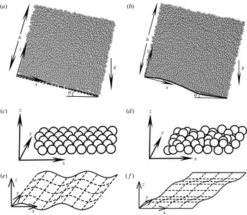
The configuration, shown in figure 1, consists of a plane inclined at an angle
 $\unicode[STIX]{x1D703}$
to the horizontal, with gravity acting vertically downward. The
 $z$
axis is perpendicular to the base, the
 $x$
axis is along the flow direction and the
 $y$
axis is in the spanwise direction. Periodic boundary conditions are used in both the flow and the spanwise directions.
The configuration and the coordinate system for analysing the flow down an inclined plane with a rough base consisting of frozen particles (a) and a base with sinusoidal height modulation in the streamwise direction (b); the base particle configuration for an ordered frozen-particle base (c) and a random frozen-particle base (d); the base configuration for sinusoidal modulation in the streamwise
 $x$
direction (e) and the spanwise
 $y$
direction (f).

2.3 Base topography
Two different types of base configuration are used here, bases made of frozen particles and sinusoidal bases.
2.3.1 Frozen-particle bases
Two types of frozen-particle base configuration, hexagonally ordered and random, are considered. Hexagonally ordered frozen-particle bases consist of a two-dimensional hexagonal close-packed array of particles, shown in figure 1(c). The results here are independent of the orientation of the sides of the hexagon with respect to the flow direction, and the results shown here are for the case where one edge of the hexagon is parallel to the flow direction. The ratio of the diameter of the base and moving particles is varied in order to modify the roughness of the base.
In order to generate a random frozen-particle base, shown in figure 1(d), particles are filled sequentially into the simulation box which is held horizontal. A slice of particles from this box, of thickness equal to two particle diameters, is used as the frozen base. The interaction parameters between the moving and frozen particles are identical to those between two flowing particles in all cases.
2.3.2 Sinusoidal bases
For the sinusoidal bases, the base height has a sinusoidal variation of the form
 $z=A\sin (2\unicode[STIX]{x03C0}x/\unicode[STIX]{x1D706})$
for modulation along the streamwise direction, shown in figure 1(e), and of the form
 $z=A\sin (2\unicode[STIX]{x03C0}y/\unicode[STIX]{x1D706})$
for modulation along the spanwise direction, shown in figure 1(f). Here,
 $A$
is the amplitude and
 $\unicode[STIX]{x1D706}$
is the wavelength. The maximum wavelength of the base modulation
 $\unicode[STIX]{x1D706}$
is equal to the simulation box length in the direction of modulation, while the minimum wavelength is equal to the diameter of the flowing particle. For the particle–base interactions, the base is considered to be a particle of infinite mass with the same interaction parameters as those for particle–particle interactions.
2.4 Dynamical and structural properties
Results for the volume fraction and velocity profiles are calculated by subdividing the granular layer into bins of height
 $0.05$
particle diameters in the base-normal (
 $z$
) direction and calculating averages over these bins. Most of the parameters reported are for the steady state, unless otherwise stated.
2.4.1 Number density and structural order parameter
The number density
 $n$
is used to distinguish between uniform flows and layered flows, where the flow consists of layers of particles sliding over each other. The number density is defined as the number of particles with centres within the bin, divided by the volume. This is, in general, different from the volume fraction
 $\unicode[STIX]{x1D719}$
, which is the fraction of the volume in the bin occupied by the particles. It should be noted that for calculating the number density and volume fraction, the bin widths in the base-normal direction are (
 $1/20$
) of the particle diameter. When the volume fraction is calculated in a differential interval for a layered state, the particle slices within the volume are included in the calculation of the volume fraction, and so the there is relatively less variation of volume fraction with height. In contrast, when the number density is calculated, the particles are counted only if their centres are within the differential interval, and these are divided by the differential volume. For layered flows, this results in a sharp peak at the bins containing the centres of the particles within a layer, and zero number density for bins that do not contain any particle centres. In contrast, for random flows where there is no layering, the number density profiles are uniform. Due to this, the number density is a discerning indicator of layering.
For layered flows, the arrangement of particles within the layers is assessed using the in-plane order parameter
 $q_{6}$
calculated in the
 $x$
–
 $y$
plane parallel to the base. The value of the order parameter
 $q_{6}$
in the interval
 $\unicode[STIX]{x0394}z$
centred at the location
 $z$
is defined as
 $$\begin{eqnarray}q_{6}=\frac{1}{N}\mathop{\sum }_{i=1}^{N}\mathop{\sum }_{j}^{\prime }\langle \exp (\imath 6\unicode[STIX]{x1D703}_{ij})\rangle ,\end{eqnarray}$$
where
 $N$
is the total number of particles with centres within the interval
 $\unicode[STIX]{x0394}z$
about
 $z$
. For each particle with centre in the interval
 $\unicode[STIX]{x0394}z$
about
 $z$
,
 $\unicode[STIX]{x1D703}_{ij}$
is the angle made by the line joining particles
 $i$
and
 $j$
in the
 $x$
–
 $y$
plane with a fixed reference. The prime in (2.9) indicates that the summation over
 $j$
is carried out over all neighbouring particles whose
 $z$
coordinate is within 0.1 particle diameters of particle
 $i$
. The order parameter
 $q_{6}$
is
 $1$
for hexagonally ordered spherical particles in two dimensions and it is 0 for a random arrangement of particles. In order to distinguish between ordered and disordered regions, a cutoff of
 $0.5$
for the
 $q_{6}$
order parameter is used – regions with
 $q_{6}$
greater than
 $0.5$
are considered to be ordered, while those with
 $q_{6}$
less than
 $0.5$
are considered to be disordered.
The three-dimensional order parameter
 $Q_{6}$
, based on the spherical harmonics, is also used to assess FCC or HCP ordering in three dimensions, but this is not employed in the present study. As reported by Kumaran & Maheshwari (Reference Kumaran and Maheshwari2012), this order parameter does not show much variation at the order–disorder transition. It is only the two-dimensional order parameter
 $q_{6}$
that shows a significant jump at the order–disorder transition, and so we only report results for
 $q_{6}$
.
2.4.2 Mean velocity, angular velocity and granular temperature
The flow velocity and angular velocity are calculated as the averages of the particle velocity and angular velocity for each height interval
 $\unicode[STIX]{x0394}z$
centred at the location
 $z$
,
 $$\begin{eqnarray}\displaystyle & \displaystyle \boldsymbol{v}=\frac{1}{N}\mathop{\sum }_{i=1}^{N}\boldsymbol{v}_{i}, & \displaystyle\end{eqnarray}$$
 $$\begin{eqnarray}\displaystyle & \displaystyle \unicode[STIX]{x1D734}=\frac{1}{N}\mathop{\sum }_{i=1}^{N}\unicode[STIX]{x1D74E}_{i}. & \displaystyle\end{eqnarray}$$
The granular temperature is defined as
 $$\begin{eqnarray}T=\frac{1}{6N}\mathop{\sum }_{i=1}^{N}\left(\frac{m(\boldsymbol{v}_{i}-\boldsymbol{v})^{2}}{2}+\frac{I(\unicode[STIX]{x1D74E}_{i}-\unicode[STIX]{x1D734})^{2}}{2}\right),\end{eqnarray}$$
where
 $m$
is the particle mass and
 $I$
is the moment of inertia.
2.4.3 Theoretical comparison
In order to assess previous theoretical predictions, the velocity and temperature profiles are compared with two types of theoretical predictions, the Bagnold profiles and more detailed kinetic models obtained from kinetic theories for dense granular flows.
The flow is considered to be fully developed, because periodic boundary conditions are used in the streamwise direction. The momentum conservation equations for a unidirectional flow at steady state are
 $$\begin{eqnarray}\displaystyle 0=\left\{\begin{array}{@{}l@{}}\displaystyle \frac{\unicode[STIX]{x2202}\unicode[STIX]{x1D70E}_{xz}}{\unicode[STIX]{x2202}z}+\unicode[STIX]{x1D70C}g_{x},\\ \displaystyle \frac{\unicode[STIX]{x2202}\unicode[STIX]{x1D70E}_{zz}}{\unicode[STIX]{x2202}z}+\unicode[STIX]{x1D70C}g_{z}.\end{array}\right. & & \displaystyle\end{eqnarray}$$
Here,
 $\unicode[STIX]{x1D70C}$
is the mass density, and
 $g_{x}$
and
 $g_{z}$
are the components of the gravitational acceleration parallel and perpendicular to the base. The components of the stress tensor,
 $\unicode[STIX]{x1D70E}_{xz}$
and
 $\unicode[STIX]{x1D70E}_{zz}$
, are considered to be of the Bagnold form,
 $$\begin{eqnarray}\displaystyle & & \displaystyle \displaystyle \unicode[STIX]{x1D70E}_{xz}=B_{xz}\left(\frac{\text{d}v_{x}}{\text{d}z}\right)^{2},\nonumber\\ \displaystyle & & \displaystyle \displaystyle \unicode[STIX]{x1D70E}_{zz}=-B_{zz}\left(\frac{\text{d}v_{x}}{\text{d}z}\right)^{2},\end{eqnarray}$$
where
 $B_{xz}$
and
 $B_{zz}$
are the Bagnold coefficients, which depend on the volume fraction. It should be noted that
 $g_{z}$
is negative in the coordinate system used in figure 1. The ratio of the Bagnold coefficients
 $(B_{xz}/B_{zz})$
is also equal to
 $|g_{x}/g_{z}|=\tan (\unicode[STIX]{x1D703})$
, where
 $\unicode[STIX]{x1D703}$
is the angle of inclination.
At steady state, the solution for the momentum conservation (2.13) is the Bagnold profile,
 $$\begin{eqnarray}v_{x}=v_{s}+\frac{5(\bar{v}-v_{s})}{3}\left(1-\left(1-\frac{z}{h}\right)^{3/2}\right),\end{eqnarray}$$
where
 $v_{s}$
is the slip velocity at the base,
 $\bar{v}$
is the height-averaged velocity and
 $h$
is the flow height. From the streamwise momentum conservation equation (2.13), the parameters in (2.15) are related to the Bagnold coefficients,
 $$\begin{eqnarray}\bar{v}-v_{s}=\frac{2\sqrt{\unicode[STIX]{x1D70C}g_{x}h^{3}}}{5\sqrt{B_{xz}}}.\end{eqnarray}$$
The strain rate is
 $$\begin{eqnarray}\frac{\text{d}v_{x}}{\text{d}z}=\frac{5(\bar{v}-v_{s})}{2}\sqrt{1-\frac{z}{h}}.\end{eqnarray}$$
The Froude number
 $Fr=(\bar{v}/\sqrt{gh})$
is
 $$\begin{eqnarray}Fr=\frac{v_{s}}{\sqrt{gh}}+\frac{2\sqrt{\unicode[STIX]{x1D70C}\sin (\unicode[STIX]{x1D703})h^{2}}}{5\sqrt{B_{xz}}}.\end{eqnarray}$$
The Froude number increases as
 $h$
as the height is increased when there is no slip, but there is also a contribution proportional to
 $h^{-1/2}$
due to the slip velocity.
For the Bagnold velocity profiles, a balance between the shear production and the inelastic dissipation results in a linear temperature variation with depth. The temperature profiles have the form
 $$\begin{eqnarray}T=T^{\prime }(h-z),\end{eqnarray}$$
where
 $T^{\prime }$
, the negative of the slope of the temperature profile, is independent of the layer height or the base configuration, and depends only on the volume fraction and the angle of inclination. It should be noted that
 $T^{\prime }h$
is the extrapolated value of the linear approximation for the temperature at the base, and not the actual temperature. The linear approximation is not valid at the base or the free surface, since there the rate of conduction of energy becomes comparable to the rates of production and dissipation.
The granular temperature and strain rate profiles facilitate a deeper comparison with continuum models based on kinetic theory. In these models, the shear stress
 $\unicode[STIX]{x1D70F}$
, pressure
 $p$
and inelastic energy dissipation rate per unit volume
 $D$
are related to the granular temperature
 $T$
and strain rate
 $(\text{d}v_{x}/\text{d}z)$
as
 $$\begin{eqnarray}\displaystyle \left.\begin{array}{@{}rcl@{}}p\ & =\ & -(p_{\unicode[STIX]{x1D719}}T/d^{3}),\\ \unicode[STIX]{x1D70F}\ & =\ & (\unicode[STIX]{x1D707}_{\unicode[STIX]{x1D719}}\sqrt{T}|\text{d}v_{x}/\text{d}z|/d^{2}),\\ D\ & =\ & (D_{\unicode[STIX]{x1D719}}T^{3/2}/d^{4}),\end{array}\right\} & & \displaystyle\end{eqnarray}$$
where
 $d$
is the particle diameter, the particle mass is considered to be
 $1$
without loss of generality, and
 $p_{\unicode[STIX]{x1D719}}$
,
 $\unicode[STIX]{x1D707}_{\unicode[STIX]{x1D719}}$
and
 $D_{\unicode[STIX]{x1D719}}$
are dimensionless functions of the volume fraction
 $\unicode[STIX]{x1D719}$
. A balance between the rates of shear production and inelastic dissipation in the bulk provides the relation
 $$\begin{eqnarray}\frac{T}{d^{2}(\text{d}v_{x}/\text{d}z)^{2}}=\frac{\unicode[STIX]{x1D707}_{\unicode[STIX]{x1D719}}}{D_{\unicode[STIX]{x1D719}}}.\end{eqnarray}$$
The Bagnold coefficients
 $B_{xz}$
and
 $B_{zz}$
can be related to the coefficients
 $p_{\unicode[STIX]{x1D719}}$
,
 $\unicode[STIX]{x1D707}_{\unicode[STIX]{x1D719}}$
and
 $D_{\unicode[STIX]{x1D719}}$
as
 $$\begin{eqnarray}\displaystyle \left.\begin{array}{@{}rcl@{}}B_{xz}\ & =\ & \displaystyle \frac{\unicode[STIX]{x1D707}_{\unicode[STIX]{x1D719}}}{d}\sqrt{\frac{\unicode[STIX]{x1D707}_{\unicode[STIX]{x1D719}}}{D_{\unicode[STIX]{x1D719}}}},\\ B_{zz}\ & =\ & \displaystyle \frac{p_{\unicode[STIX]{x1D719}}\unicode[STIX]{x1D707}_{\unicode[STIX]{x1D719}}}{dD_{\unicode[STIX]{x1D719}}}.\end{array}\right\} & & \displaystyle\end{eqnarray}$$
One relation between
 $p_{\unicode[STIX]{x1D719}}$
,
 $\unicode[STIX]{x1D707}_{\unicode[STIX]{x1D719}}$
and
 $D_{\unicode[STIX]{x1D719}}$
is obtained from the requirement that the ratio of the shear and normal stresses is the tangent of the angle of inclination,
 $$\begin{eqnarray}\tan (\unicode[STIX]{x1D703})=\frac{\sqrt{\unicode[STIX]{x1D707}_{\unicode[STIX]{x1D719}}D_{\unicode[STIX]{x1D719}}}}{p_{\unicode[STIX]{x1D719}}}.\end{eqnarray}$$
A more detailed ‘thermal boundary layer’ model (Kumaran Reference Kumaran2008) predicts the form of the temperature near the base as
 $$\begin{eqnarray}T=T^{\prime }\left(h\frac{(1-c\exp (-z/\unicode[STIX]{x1D6FF}))^{2}}{(1+c\exp (-z/\unicode[STIX]{x1D6FF}))^{2}}-z\right),\end{eqnarray}$$
where
 $\unicode[STIX]{x1D6FF}$
is a ‘thermal boundary layer thickness’, which depends only on flow properties and is independent of the base topography, and
 $c$
is a constant that depends on the rate of input or dissipation of energy at the base. In Kumaran (Reference Kumaran2008), it was proposed that the constant
 $c$
can be determined from the temperature boundary condition at
 $z=0$
,
 $$\begin{eqnarray}\frac{\text{d}T}{\text{d}z}=\unicode[STIX]{x1D6FD}T,\end{eqnarray}$$
where the parameter
 $\unicode[STIX]{x1D6FD}$
, which is the inverse of a ‘slip length’ for the temperature, is related to
 $c$
and the boundary layer thickness through the relation
 $$\begin{eqnarray}\unicode[STIX]{x1D6FD}=\frac{4c}{(1-c^{2})\unicode[STIX]{x1D6FF}}.\end{eqnarray}$$
In the derivation of (2.26), terms of
 $O(\unicode[STIX]{x1D6FF}/h)$
are neglected due to the assumption that the boundary layer thickness is much smaller than the total height.
It is important to note that in the theory of Kumaran (Reference Kumaran2008), the thermal boundary layer thickness is independent of the layer height and the base configuration, and depends only on the bulk volume fraction in the flowing layer. The constant
 $c$
does depend on the details of the base configuration: the constant
 $c$
is positive for a dissipative base with an outflow of energy at the base and negative when there is an energy input at the base. However, the ratio of the temperature and the square of the strain rate,
 $(T/d^{2}(\text{d}v_{x}/\text{d}z)^{2})$
, is a constant in the boundary layer even when the temperature and strain rate depart from the bulk scaling. The temperature profiles are compared with (2.19) and (2.24), and the ratio of the temperature and the square of the stain rate is also examined, to assess the applicability of the thermal boundary layer approximation at the base.
3 Results
In this section, the mass, length and time dimensions are scaled by the particle mass, the particle diameter
 $d$
and
 $\sqrt{d/g}$
respectively, where
 $g$
is the acceleration due to gravity. Dimensionless variables are used to report all results. The dimension of the simulation box along the flow direction is 40–160 particle diameters and in the spanwise direction it is 20–40 particle diameters. Layers with heights of 18–70 particle diameters are simulated, and the angle of inclination is
 $22^{\circ }$
in all cases. Results are presented for one of two layer heights, approximately 35 particle diameters and approximately 70 particle diameters, unless otherwise stated.
The simulations are carried out starting with a horizontal static configuration prepared by sequentially adding particles to the base and then tilting the configuration to an angle of
 $22^{\circ }$
to initiate flow. The dimensionless time step in the simulations is
 $4\times 10^{-5}$
. The simulations are run for approximately 800 time units to reach steady state, and then average properties are calculated over production runs comprising four different sequences, each consisting of 1000 configurations recorded over 8 time units. The mean value and the standard deviation are reported for all of the primary measurements, the mean velocity (figure 7), the angular velocity (figure 9) and the granular temperature (figure 10). The mean value is the average over the entire production run of 32 time units, while the standard deviation (shown by the error bars) is determined from the average values for each of the four subsequences of 8 dimensionless time units. The standard deviation in the mean velocity measurements (shown in figure 7) is approximately 1 % of the maximum velocity. There is a larger standard deviation of approximately 10 % in the granular temperature, although the error bars in figure 10 appear to be much smaller due to the logarithmic scale used. There is a standard deviation of approximately 10 % in the measurement of the angular velocity as well, as shown in figure 9.
3.1 Transition
A transition from an ordered to a disordered flowing state is observed for all of the different base configurations studied here when the base amplitude is increased beyond a critical value. For the random base, it has been reported (Kumaran & Maheshwari Reference Kumaran and Maheshwari2012; Kumaran & Bharathraj Reference Kumaran and Bharathraj2013) that the transition takes place when
 $d_{b}$
, the base particle diameter, is increased from
 $0.57$
to
 $0.58$
. Here, the order–disorder transition is also observed for the hexagonal close-packed base when
 $d_{b}$
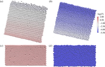
is increased from 1.34 to 1.35, independent of layer height, as shown in figure 2. When the base amplitude is 1.34 or lower, the flow is clearly layered, as shown in side view in figure 2(a), and there is in-plane hexagonal ordering, as shown in the top view in figure 2(c). When the base particle diameter is increased to
 $1.35$
, there is an abrupt transition to a disordered flow with no visible layering, as shown in the side view in figure 2(b), and no crystalline ordering in-plane, as shown in the top view in figure 2(d). The qualitative features of the flow remain unchanged when the base amplitude is increased beyond 1.35 and when the flow height is increased to approximately 70 particle diameters. We have also verified that the qualitative features remain unchanged when the length and width of the simulation box are increased by a factor of
 $2$
, and so this is not a finite size effect. These qualitative features are also identical to those observed for the rough base in Kumaran & Maheshwari (Reference Kumaran and Maheshwari2012), Kumaran & Bharathraj (Reference Kumaran and Bharathraj2013).
Side view in the
 $x$
–
 $z$
plane, (a) and (b), and view from above in the
 $x$
–
 $y$
plane though the centre of the flowing layer, (c) and (d), of a configuration of flowing particles on an ordered frozen-particle base with base particle diameter
 $1.34$
(a,c) and
 $1.35$
(b,d). The simulation cell has a length of 40 particle diameters in the flow (
 $x$
) direction and 20 particle diameters in the spanwise (
 $y$
) direction, and a height of approximately 35 particle diameters. The side images are colour coded according to the logarithm of the granular temperature, as shown by the colour bar.

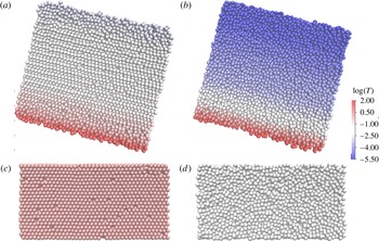
Transition is also observed for sinusoidal bases. An example is shown in figure 3 for a sinusoidal base with modulation in the flow direction with a wavelength of
 $40$
particle diameters and a height of approximately 35 particle diameters. When the base amplitude is increased from 0.48 to 0.49, there is a discontinuous change from an ordered to a disordered flow. There is no change in the particle configuration and flow dynamics when the amplitude is increased above 0.49 in the disordered flow, or when the amplitude is decreased below 0.48 in the ordered flow. These qualitative features are observed for all other wavelengths of base modulation in both the streamwise and the spanwise directions, although the transition amplitude does depend on the wavelength, the direction of modulation and the height of the layer. These qualitative features also remain unchanged when the length or width of the simulation box is increased by a factor of
 $2$
, indicating the lack of system-size dependence.
Side view in the
 $x$
–
 $z$
plane, (a) and (b), and view from above in the
 $x$
–
 $y$
plane though the centre of the flowing layer, (c) and (d), of a configuration of flowing particles on a sinusoidal base with amplitude
 $A=0.48$
(a,c) and
 $0.49$
(b,d). The wavelength of the modulation is 40 particle diameters in the streamwise (
 $x$
) direction, the simulation cell has a length of 40 particle diameters in the flow (
 $x$
) direction and 20 particle diameters in the spanwise (
 $y$
) direction, and a height of approximately 35 particle diameters. The side images are colour coded according to the logarithm of the granular temperature, as shown by the colour bar.

Although the salient features of the ordered and disordered flows appear to be the same for sinusoidal and frozen-particle bases, a closer comparison of figures 2 and 3 reveals important differences. In the ordered flow over an ordered frozen-particle base, there is ordering and layering down to the base, as shown in figure 2(a). Both ordered and random frozen-particle bases exhibit ordering down to the base, unless the base particle diameter decreases below a critical value, as discussed in § 3.4. For ordered flows over sinusoidal bases, there is a region of height of approximately 5 particle diameters where the particle configuration is disordered. This disordered region at the bottom is observed for all sinusoidal bases, regardless of the wavelength or direction of modulation.
The second important difference is in the granular temperature for ordered and disordered flows, shown by the colour gradation in figures 2 and 3. It should be noted that the common colour bar in both figures indicates the logarithm of the granular temperature. The granular temperature for the ordered flow is significantly higher than that for the disordered flow, by approximately one order of magnitude, as discussed in § 3.4. A second important difference is the significant increase in the granular temperature at the base for flows over sinusoidal bases in figure 3, which is noticeably absent for flows over the frozen-particle base in figure 2. In the former, the region of very high temperature for the ordered flow coincides with region of height approximately 5 particle diameters where the particle configuration is disordered. As we show in §§ 3.3 and 3.4, this basal disordered region is a region of high granular temperature and strain rate, and flows with a bottom disordered region also exhibit large slip velocities and large angular velocities at the base. The basal region of very high temperature and strain rate is also present for disordered flows over sinusoidal bases, but is absent for disordered flows over frozen-particle bases, as discussed in §§3.3 and 3.4.
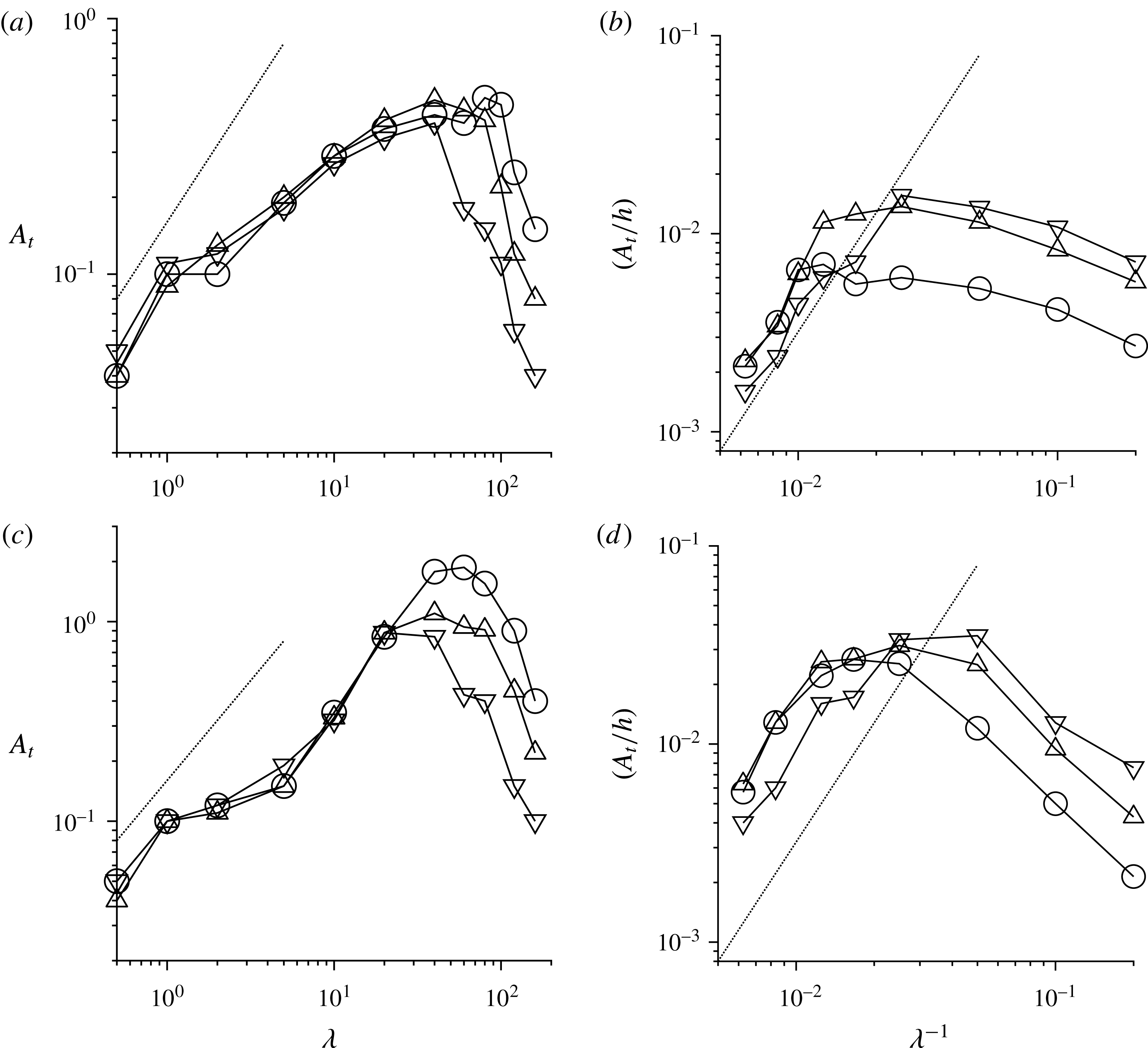
The transition amplitude is shown as a function of the wavelength of perturbations
 $\unicode[STIX]{x1D706}$
in figure 4 for modulation in the streamwise and spanwise directions. The transition amplitude for the spanwise modulation is larger than that for the streamwise modulation, and it shows a larger increase with system height. However, there are some common features for both streamwise and spanwise modulations. The transition amplitude initially increases as the wavelength increases, reaches a maximum and then decreases with further increase in the wavelength. The initial increase in transition amplitude is independent of the height of the layer to within the uncertainties of 1 % in the simulation, but the location of the maximum increases with layer height. The transition amplitude increases proportional to
 $\unicode[STIX]{x1D706}$
, and is independent of layer height, in the limit of small
 $\unicode[STIX]{x1D706}$
, as shown in figure 4(a,c). In the opposite limit of long wavelength, the transition amplitude seems to decrease proportional to
 $(h/\unicode[STIX]{x1D706}^{2})$
, where
 $h$
is the layer height, as shown in figure 4(b,d).
The transition amplitude
 $A_{t}$
as a function of the wavelength of the sinusoidal base modulation
 $\unicode[STIX]{x1D706}$
(a,c), and
 $(A_{t}/h)$
as a function of the inverse of the wavelength
 $\unicode[STIX]{x1D706}^{-1}$
(b,d). Panels (a) and (b) show the results for a base with modulation in the streamwise (
 $x$
) direction, shown in figure 1(e), and panels (c) and (d) show the results for modulation in the spanwise (
 $y$
) direction, shown in figure 1(f). The heights of the flowing layer are approximately
 $25$
(▿),
 $35$
(▵) and
 $70$
(○). The dotted line in (a) indicates a slope of
 $+1$
on a log–log graph, and the dotted line in (b) indicates a slope of
 $+2$
.

3.2 Particle configuration
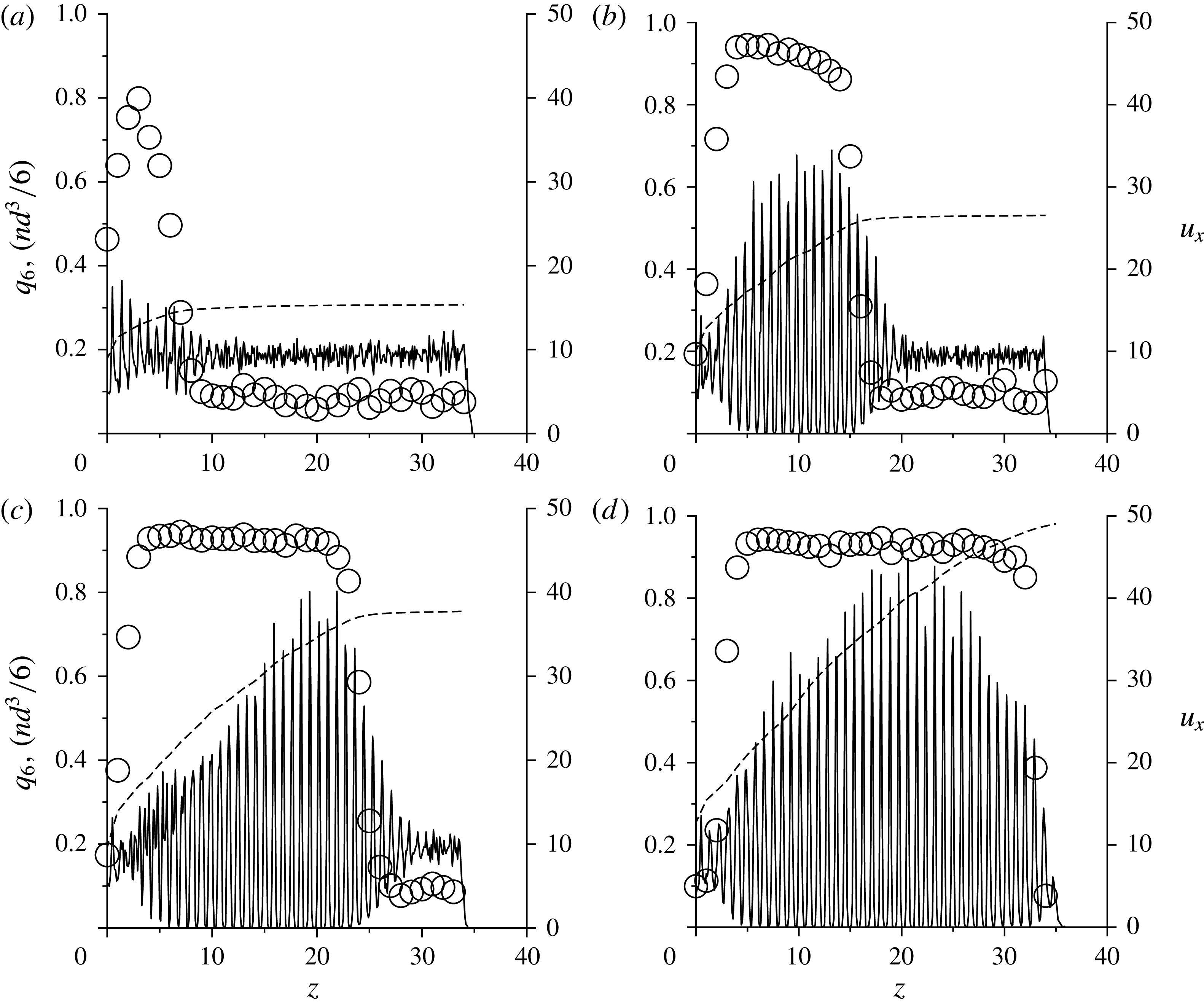
The structural features are quantified and compared in figures 5 and 6 for a layer height of approximately 35 particle diameters. Here, the number density and the
 $q_{6}$
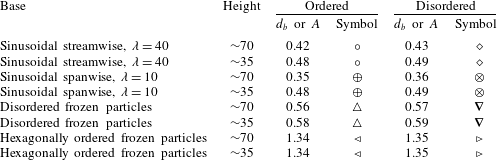
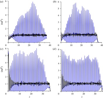
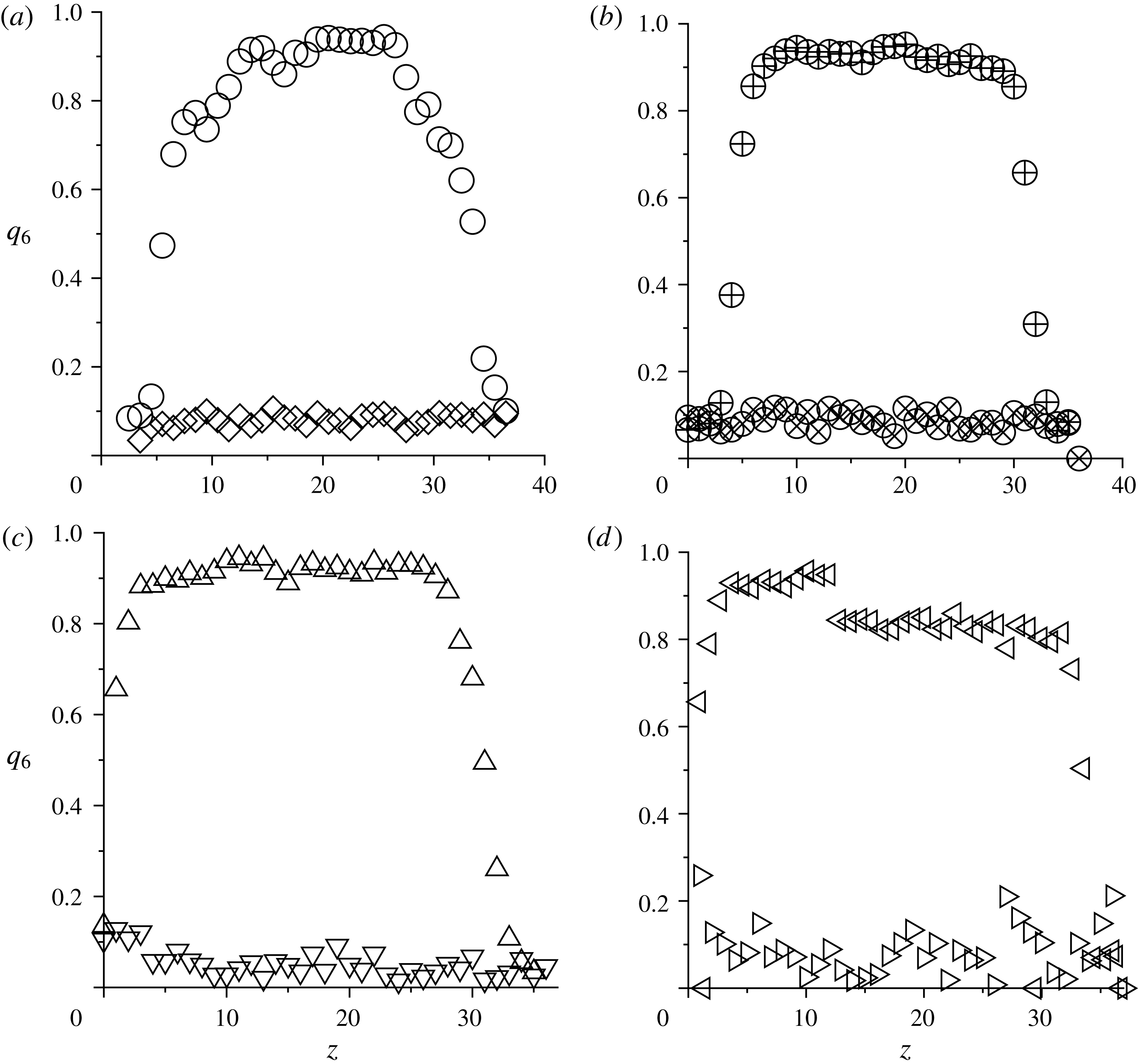
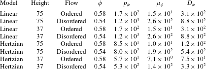
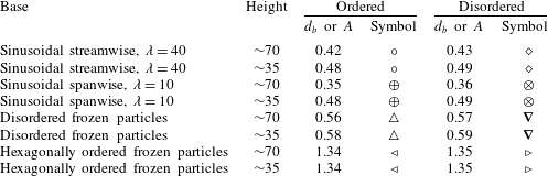
order parameter are plotted as a function of height for different base amplitudes for two different values of the base roughness, the first for an ordered flow and the second for a disordered flow. The parameters used in the figures for different types of base roughness are shown in table 1. The transition between the ordered and disordered flow is clearly visible in the number density profiles. In the ordered flow, the number density
 $n$
exhibits an oscillatory variation with height, as shown in figure 5, with a maximum value in the range 4–6 at the location of the centres of the particles in the layers and a minimum value close to zero midway between the centres. The spacing between the layers is a little less than
 $1$
particle diameter. In the disordered flow, no layering is visible, and the number density is close to its average value throughout the height. The profiles of the
 $q_{6}$
order parameter in figure 6 show that layering is accompanied by in-plane hexagonal ordering. In the ordered flow, the
 $q_{6}$
order parameter is greater than 0.8, indicating near-perfect hexagonal ordering within the layers for all types of base roughness. In the disordered flow, the
 $q_{6}$
order parameter is less than 0.2 in all cases. The coordination number, not shown here, does not change significantly at transition. Thus, figures 5 and 6 show that the behaviour in the bulk is independent of the type of base roughness in both the ordered and the disordered flows, although the structural features do change discontinuously when there is a transition between the ordered and the disordered flows.
The amplitude of the sinusoidal perturbations
 $A$
for the sinusoidal bases and the base particle diameter
 $d_{b}$
for the disordered and ordered frozen-particle bases considered in figures 5–11, 16 and 18. The transition amplitudes are the same for the linear and Hertzian contact models. In all figures, the angle of inclination is
 $22^{\circ }$
and the simulation cell has a length of 40 particle diameters in the flow (
 $x$
) direction and 20 particle diameters in the spanwise (
 $y$
) direction.
The variation of the number density
 $n$
as a function of the height
 $z$
for the flow of a layer of particles of height approximately 35 particle diameters above (a) a sinusoidal base with modulation in the flow (
 $x$
) direction, (b) a sinusoidal base with modulation in the spanwise (
 $y$
) direction, (c) a hexagonally ordered frozen-particle base and (d) a random frozen-particle base. The base amplitude and the base particle diameter corresponding to the different symbols for the number density profiles are shown in table 1. In each panel, the thick black line shows the number density for the disordered flow and the thin blue line shows the number density for the ordered flow.

The
 $q_{6}$
order parameter as a function of the height
 $z$
for the flow of a layer of particles of height approximately 35 particle diameters above (a) a sinusoidal base with modulation in the flow (
 $x$
) direction, (b) a sinusoidal base with modulation in the spanwise (
 $y$
) direction, (c) a hexagonally ordered frozen-particle base and (d) a random frozen-particle base. The base amplitude and the base particle diameter corresponding to the different symbols for the
 $q_{6}$
profiles are shown in table 1.

There are systematic variations within regions of thickness 5–10 particle diameters at the base when the type of base roughness is changed, as shown in figures 5 and 6. For a sinusoidal base, the layering is not perfect within a region of thickness approximately 5–10 particle diameters at the base, as shown in figure 5(a,b), and the value of
 $q_{6}$
is also significantly smaller than
 $1$
in this region, as shown in figure 6(a,b). It should be noted that the amplitude of the sinusoidal base is less than
 $0.5$
times the particle diameter, and so it is much smaller than the thickness of the layer of approximately 5 particle diameters with imperfect ordering. This disordered layer at the bottom is observed for all of the sinusoidal bases considered here, for modulation in the streamwise and spanwise directions. For the random and hexagonally ordered frozen-particle bases, layering is observed (figure 5
c,d), and the
 $q_{6}$
order parameter is close to 1 (figure 6
c,d) even at the base. In fact, incipient ordering is observed at the frozen-particle base even for a disordered flow. These features are qualitatively similar for both random and hexagonally ordered frozen-particle bases. Thus, there are two distinct classes of basal flow, the first for frozen-particle bases, where ordering is observed down to the base, and the second for sinusoidal bases, where there is a disordered region near the base.
The details of the mean velocity, angular velocity and temperature profiles for flows over frozen-particle and sinusoidal bases are discussed next. The results for the velocity and temperature profiles are shown only for the simulations with a layer height of approximately 70 particle diameters; the results for a layer height of 35 particle diameters are qualitatively similar, and so they are not shown here.
3.3 Mean velocity and angular velocity
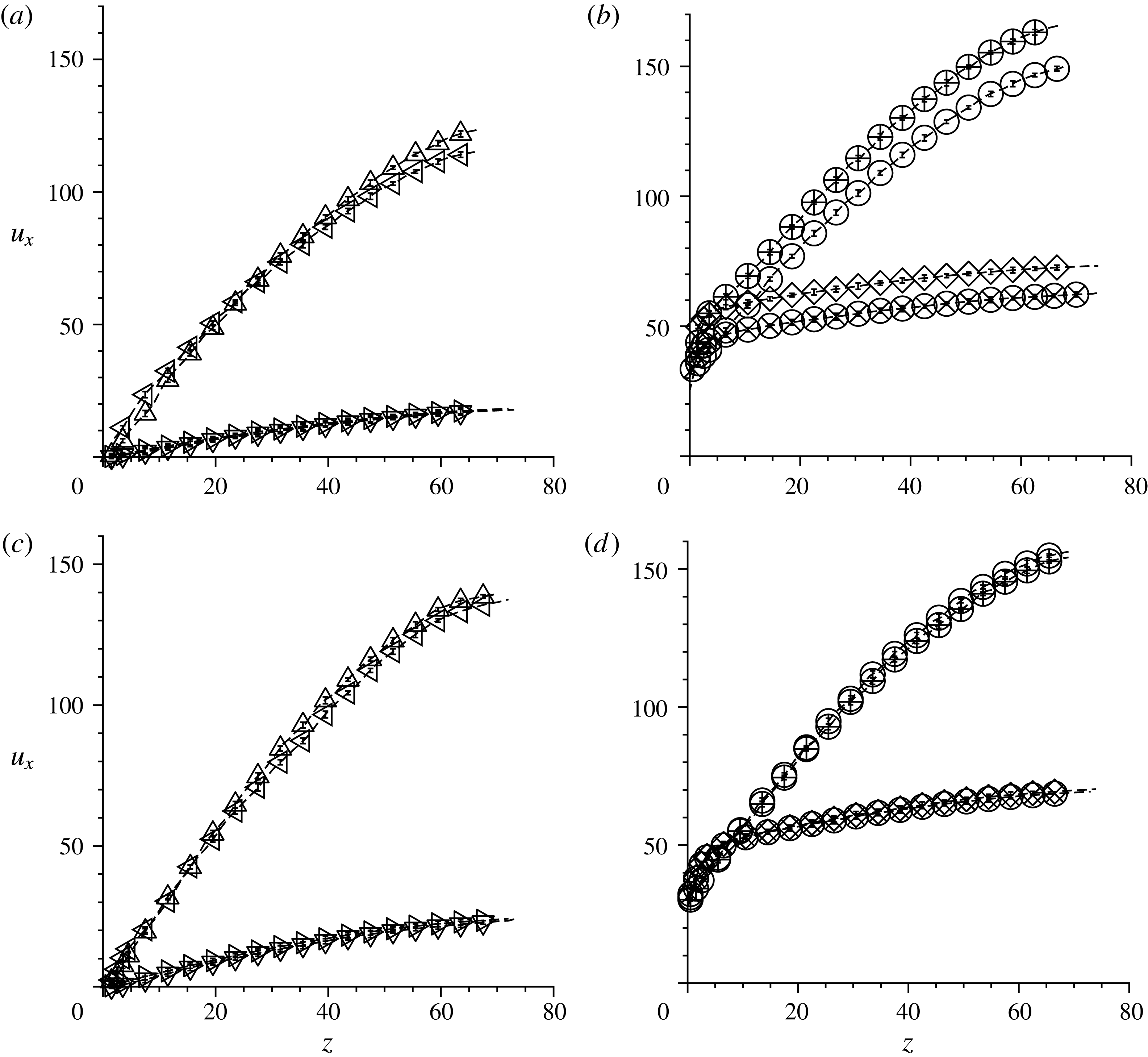
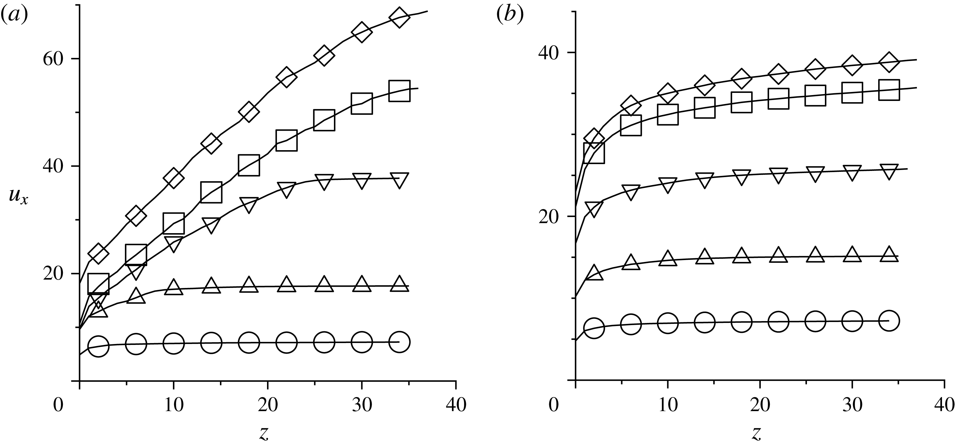
The transition is reflected in the mean velocity profiles, shown in figure 7. The mean velocity for an ordered flow exceeds that for a disordered flow by one order of magnitude, even though the base amplitude or the base particle diameter differs only by 1 %. For example, for the frozen-particle base with hexagonally ordered particles, our simulations show that there is little change in the velocity profile when the base particle diameter is increased from 1.35 to 2.00. Similarly, there is little change in the mean velocity profile when the base particle diameter is decreased from 1.34 to 0.5, apart from a visible slip velocity at the base. However, there is a dramatic increase in the mean velocity when the base particle diameter is decreased from 1.35 to 1.34 in figure 7(a,c). This coincides with the layering in the bulk, and in-plane ordering, for both the linear and the Hertzian contact models. Similarly, for the rough frozen-particle bases, there is a 10-fold increase in the mean velocity when the base particle diameter is decreased from 0.57 to 0.56, as shown in figure 7(a,c) for both the frozen-particle bases. For the sinusoidal bases as well, a decrease in the base amplitude of 1 % results in a 10-fold increase in the mean velocity, as shown in figures 7(b,d). This phenomenon is consistently observed for all of the base configurations, for both the contact models used here, and is independent of height or angle of inclination.
Mean velocity profiles for the flow over frozen-particle bases (a,c) and sinusoidal bases (b,d) for the linear contact model (a,b) and the Hertzian contact model (c,d) for a height of approximately 70 particle diameters. The type of base roughness and the parameter values for the different symbols are provided in table 1.

In the bulk of the flow, when the height exceeds approximately
 $10$
times the base particle diameter, in either the ordered or disordered flow, all velocity profiles have the same shape for all of the base configurations considered here, apart from a vertical shift due to differences in the slip velocity at the base. However, closer to the base, there are significant differences in the mean velocity profiles for different base configurations. For the frozen-particle bases, there is virtually no slip at the base for the ordered or disordered flow. In contrast, for sinusoidal bases, there is significant slip at the base for both disordered and ordered flows. In fact, the slip at the base for a disordered flow appears to be larger than that for an ordered flow. A closer look at the velocity profiles for the flow over sinusoidal bases also reveals a clear discontinuity in the slope of the velocity profile in the region within approximately 5–10 particle diameters from the base for both ordered and disordered flows. The shear rate at the base is much higher than that in the bulk, and this high shear is related to the presence of a disordered layer at the base for the ordered flow over sinusoidal bases, shown in figure 3. This bottom disordered layer with high shear rate is not present for flow over frozen-particle bases.
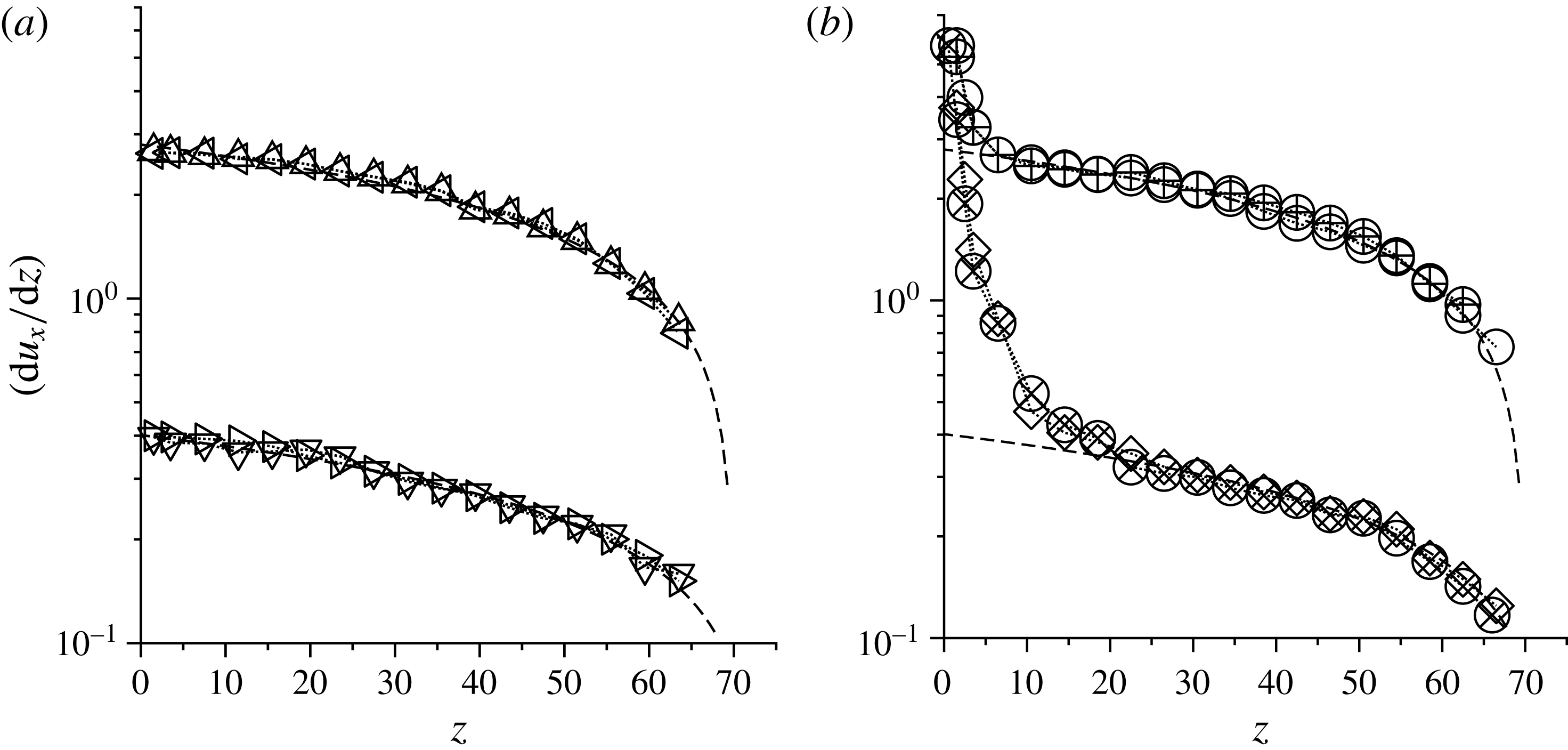
The two distinct features, the slip velocity and the large shear rate at the base, are now considered separately. The strain rate obtained from the mean velocity profiles is shown as a function of height in figure 8 for the linear contact model. The results are qualitatively similar for the Hertzian contact model. The strain rate is shown on a logarithmic scale to accommodate the large increase in the strain rate at the bottom. The Bagnold fits obtained from (2.17) for the strain rate in the bulk for the ordered and disordered flows are shown by the dashed lines. It is evident that the Bagnold profile provides a good fit for the observed velocity profiles in the bulk for both the ordered and the disordered flows. The value of the Bagnold coefficient is independent of the base configuration and depends only on the type of flow (ordered or disordered) and the angle of inclination.
Strain rate profiles for the linear contact model for flow over frozen-particle bases (a) and sinusoidal bases (b) for a height of approximately 70 particle diameters. The dashed lines are fits of (2.17). The type of base roughness and the parameter values for the different symbols are provided in table 1.

Figure 8 shows that the base topography has a significant effect on the shear rate within a region of thickness of approximately 5–10 particle diameters at the base. In the case of sinusoidal bases, there is a significant increase in the strain rate by a factor of approximately 3 in comparison with that in the bulk for an ordered flow, and by approximately one order of magnitude in comparison with the bulk strain rate for the disordered flow. This large strain rate is not observed for random and hexagonally ordered frozen-particle bases. For ordered flows over sinusoidal bases, the region of high shear rate coincides with the disordered region at the bottom discussed in § 3.2, where the granular temperature is significantly higher than that in the bulk, as discussed later in § 3.4.
Due to the mean shear, the particles have a non-zero angular velocity in the spanwise (
 $y$
) direction. If the particle rotation rate is equal to the material rotation rate, the mean angular velocity
 $\unicode[STIX]{x1D6FA}_{y}$
has to be equal to one-half of the local vorticity
 $-(\text{d}u_{x}/\text{d}z)$
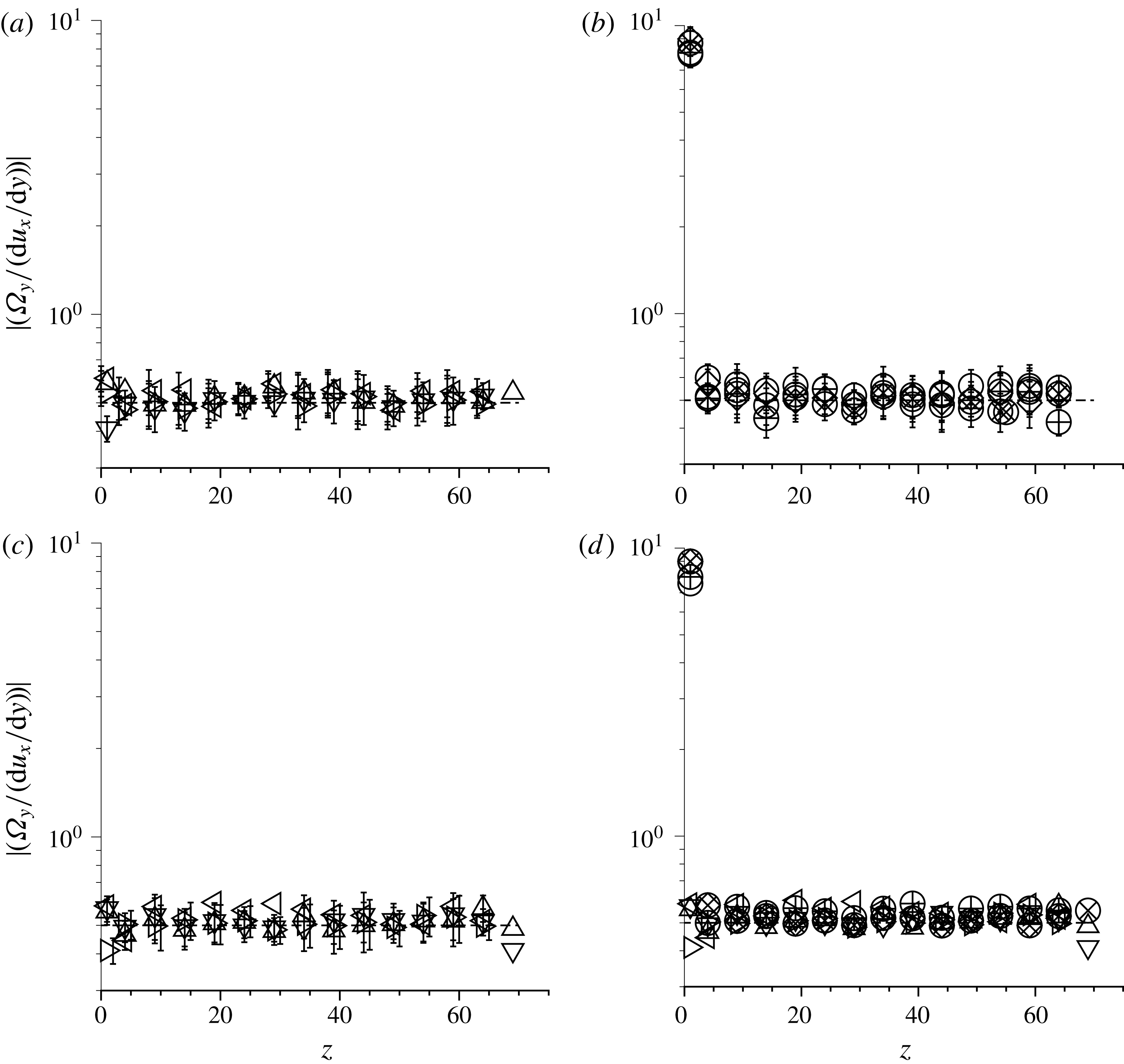
for the unidirectional flow under consideration. Instead of showing the variation of the angular velocity with height, we show the ratio
 $|(\unicode[STIX]{x1D6FA}_{y}/(\text{d}u_{x}/\text{d}z))|$
as a function of height in figure 9. It is clear that except at the bottom, this ratio is approximately 0.5 throughout the height. Even for sinusoidal bases, where there is significant slip at the base and a significant deviation from the Bagnold rheology within a region of approximately 10 particle diameters at the base, the ratio of the angular velocity and the strain rate is close to
 $0.5$
. Thus, the particle and material rotation rates are approximately equal throughout the flow, with the exception of the layer of particles closest to the base, as discussed next.
The ratio of the angular velocity and the magnitude of the strain rate for the linear contact model (a,b) and the Hertzian contact model (c,d) for a height of approximately 70 particle diameters for flow over frozen-particle bases (a,c) and sinusoidal bases (b,d). The type of base roughness and the parameter values for the different symbols are provided in table 1.

Figure 9 also shows that the ratio
 $|(\unicode[STIX]{x1D6FA}_{y}/(\text{d}u_{x}/\text{d}z))|$
is significantly different from 0.5 for the particle layers closest to the base only for sinusoidal bases. The deviations are also correlated with the presence/absence of velocity slip at the base in figure 7. For sinusoidal bases, where there is significant slip at the base and the strain rate is significantly higher than that predicted by Bagnold rheology, we find that the angular velocity is significantly higher than one-half of the vorticity. In contrast, for frozen-particle bases with no slip velocity at the base, the angular velocity is approximately one-half of the strain rate at the bottom. This suggests the presence of 1–2 layers of rapidly spinning particles at the base for sinusoidal bases; this layer of spinning particles is not present for frozen-particle bases, where there is no basal slip and where the strain rate at the base is comparable to that in the bulk. These characteristics are also correlated with a significant increase in the granular temperature at the base, which is discussed next in § 3.4.
3.4 Granular temperature
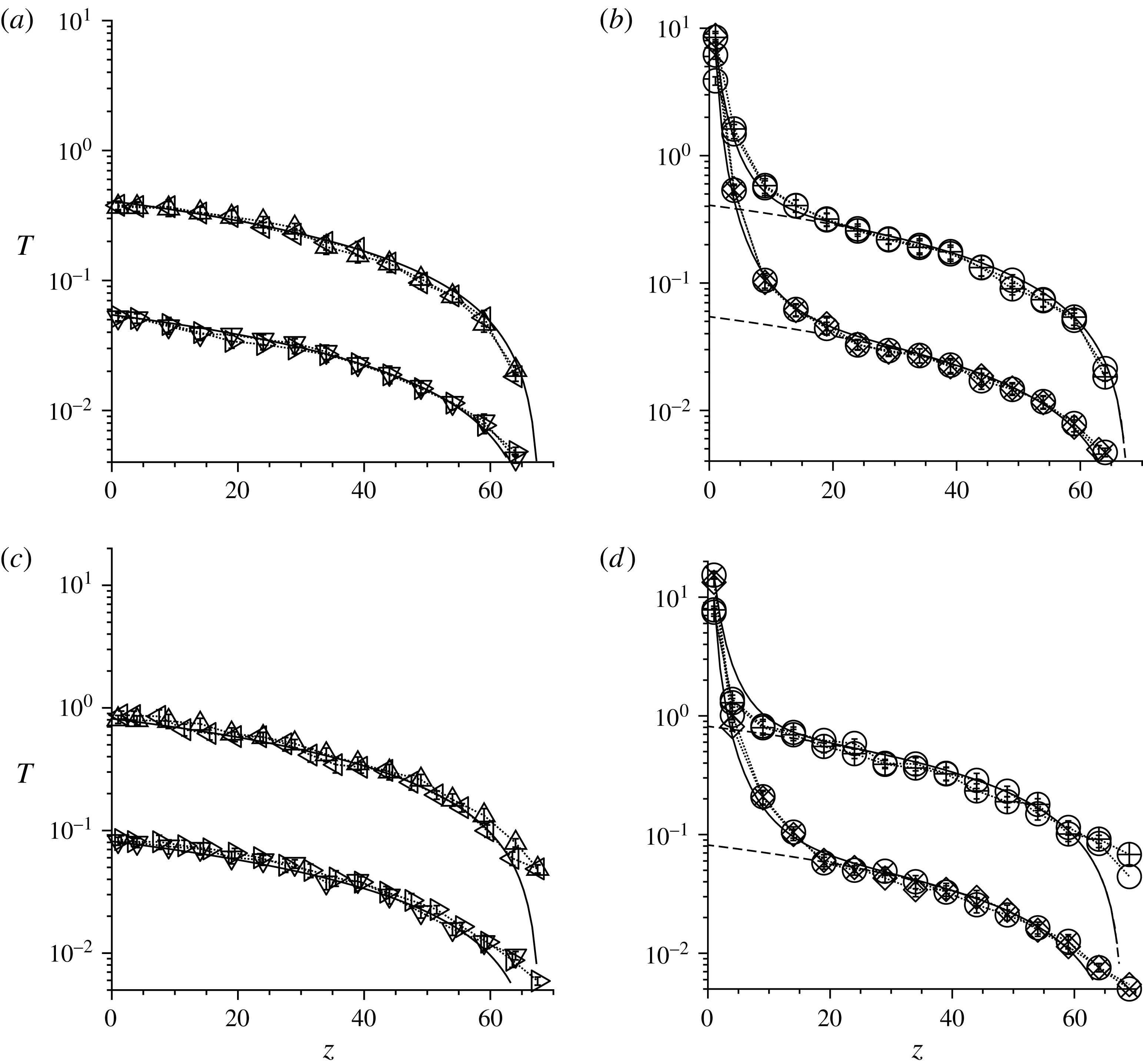
In figure 10, the granular temperature profiles for the flow over different base configurations and for equal flow heights are superposed, for both the ordered and the disordered flows. The temperature is shown on a logarithmic scale in order to accommodate the variation of decades in the temperature from the bottom to the top. In the bulk of the flow, at heights greater than approximately 10 particle diameters from the base, all temperature profiles coincide for ordered and disordered flows. For comparison, the linear temperature profiles predicted by (2.19) are shown by the dashed curves. It is apparent that the temperature profiles are well approximated by the linear profiles for both ordered and disordered flows in the bulk, but the temperatures in the ordered flow are higher, by an order of magnitude, in comparison with those in the disordered flow. This establishes that the temperature in the bulk is independent of the type of base roughness, base amplitude/wavelength or layer height, and depends only on the angle of inclination and on whether the flow is ordered or disordered.
Granular temperature profiles for the linear contact model (a,b) and the Hertzian contact model (c,d) for flow over frozen-particle bases (a,c) and sinusoidal bases (b,d) for a layer height of approximately 70 particle diameters. The dashed lines are fits of the linear relationship (2.19) and the solid lines are fits of (2.24). The type of base roughness and the parameter values for the different symbols are provided in table 1.

Figure 10(b,d) also shows that there could be a significant departure from the linear scaling at the base for sinusoidal bases. For both random and hexagonally ordered frozen-particle bases, the temperature at the base is close to the linear fit for the disordered and ordered flows, as shown in figure 10(a,c). However, for the sinusoidal bases, the temperature at the base is one order of magnitude higher than that predicted by a linear extrapolation in the ordered flow, and two orders of magnitude higher than the extrapolated linear fit in the disordered flow. This behaviour is observed for all sinusoidal bases with modulation in the streamwise and spanwise directions. This implies significantly enhanced agitation at the base, which is consistent with the observation of a significantly higher strain rate at the base in figure 7 for sinusoidal bases. For the ordered flow, the region of large temperature and strain rate at the bottom is also disordered, as shown in figure 3. However, this significant increase in temperature is not restricted to ordered flows alone, but is also observed for the disordered flows. Thus, this large temperature increase at the base seems to be a feature of the gently varying sinusoidal base topography, and is not present in the more irregular topography of random and ordered frozen-particle bases.
The ratio
 $(T/(\text{d}u_{x}/\text{d}z)^{2})$
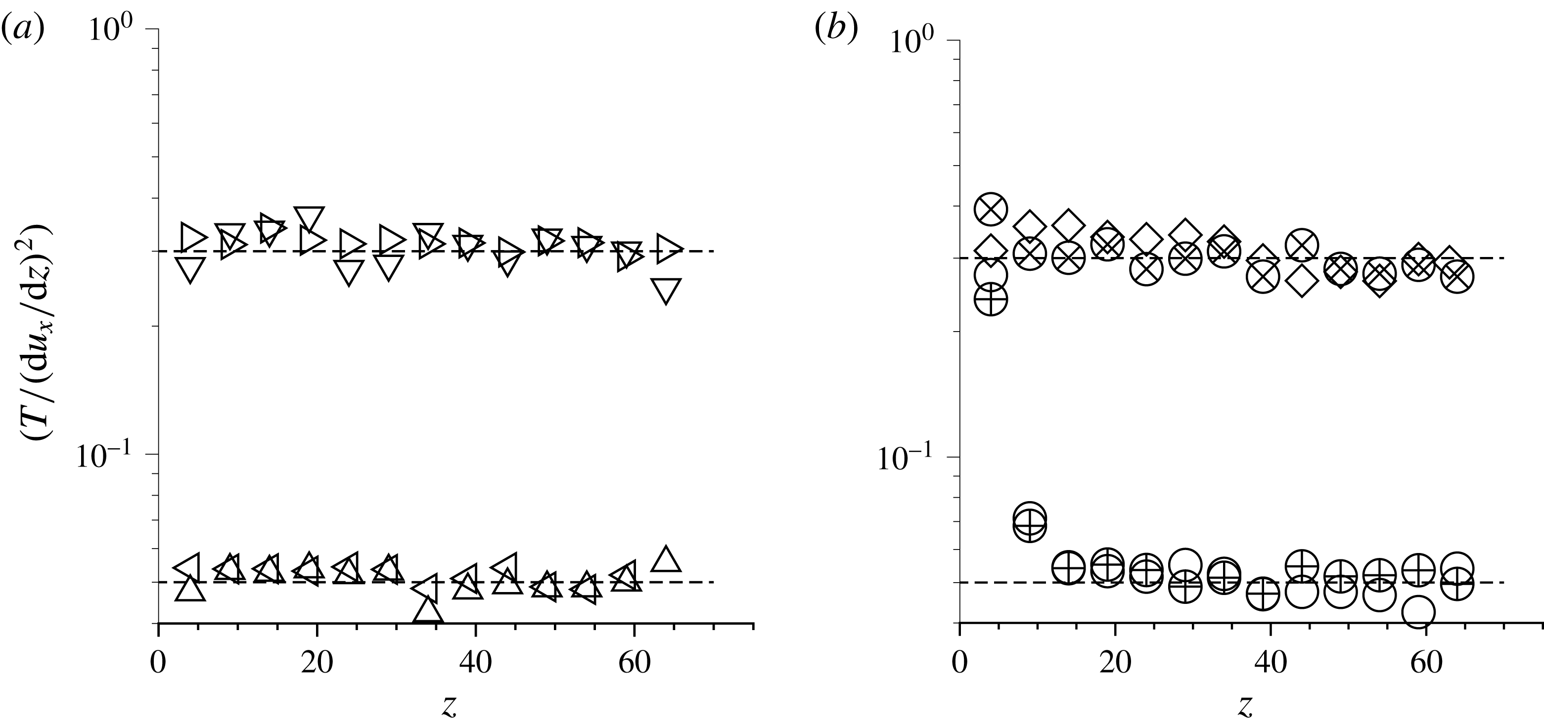
is shown as a function of height in figure 11 for the linear contact model. The results are qualitatively similar for the Hertzian contact model. This ratio provides an indication of the applicability of kinetic models based on the hard-particle approximation, since these models predict that this ratio is a constant in the bulk. There is significant scatter in the value of
 $(T/(\text{d}u_{x}/\text{d}z)^{2})$
in figure 11, due to uncertainties in the measurements of the temperature and the strain rate. Subject to these uncertainties, figure 11 does show that the ratio
 $(T/(\text{d}u_{x}/\text{d}z)^{2})$
does not vary with height in the bulk in all cases. The value is higher, by approximately an order of magnitude, for the disordered flow in comparison with the ordered flow. This is because figures 8 and 10 show that both the strain rate and the temperature in the ordered flow are approximately one order of magnitude higher than those in the ordered flow, and so the ratio in the ordered flow is approximately one order of magnitude lower. For the disordered flow, the ratio
 $(T/(\text{d}u_{x}/\text{d}z)^{2})$
in the basal layer is also the same as that in the bulk, even though there is an increase of two orders of magnitude in the granular temperature. This is consistent with one of the salient predictions of Kumaran (Reference Kumaran2008), that the ratio
 $(T/(\text{d}u_{x}/\text{d}z)^{2})$
is independent of height, even in the basal region where the granular temperature is affected by the temperature boundary condition at the base. For the ordered flow, the ratio
 $(T/(\text{d}u_{x}/\text{d}z)^{2})$
is a constant independent of height for frozen-particle bases. However, for sinusoidal bases, the value of
 $(T/(\text{d}u_{x}/\text{d}z)^{2})$
increases when the height becomes less than approximately 5 particle diameters from the base, and it approaches the value for a disordered flow at the base. This is consistent with the observation that for ordered flows over sinusoidal bases, there is a disordered region close to the base. The local value of
 $(T/(\text{d}u_{x}/\text{d}z)^{2})$
does depend on the extent of ordering in the flow, and the kinetic model with volume-fraction-dependent coefficients cannot be used when there is a spatial variation in the extent of ordering.
The ratio of the granular temperature and the square of the strain rate for the linear contact model for flow over frozen-particle bases (a) and sinusoidal bases (b) for a height of approximately 70 particle diameters. The type of base roughness and the parameter values for the different symbols are provided in table 1.

The solid lines in figure 10 show fits to the profile equation (2.24). In figure 10, one common value of the parameter
 $\unicode[STIX]{x1D6FF}$
,
 $\unicode[STIX]{x1D6FF}=4.0$
, is used for all of the ordered flows, and one common value,
 $\unicode[STIX]{x1D6FF}=5.55$
, is used for all of the disordered flows. The parameter
 $\unicode[STIX]{x1D6FF}$
is the temperature boundary layer thickness or the length scale for decay of the temperature perturbations due to the base. This value is found to be in the range 4–6 particle diameters, and is consistent with the thickness of the disordered region over sinusoidal bases in § 3.2. The value of the constant
 $c$
is, however, different for different base roughnesses. The value of
 $c$
used in figure 10 is
 $-0.8$
for an ordered flow over a sinusoidal base and
 $-0.995$
for a disordered flow over a sinusoidal base. The same parameters provide good fits for both the linear and the Hertzian models, and for the two different flow heights considered here, for disordered flows. This is in accordance with the predictions of boundary layer theories for granular flows, where the boundary layer thickness is independent of the details of the base roughness, but the boundary condition for the temperature at the base does depend on the details of the boundary roughness. However, the numerical value of the parameter
 $\unicode[STIX]{x1D6FD}$
in (2.26) is rather large in magnitude, approximately
 $-72$
, for disordered flows. Figure 10 shows that the increase in temperature at the base is not well captured for ordered flows. This is because of the presence of a disordered basal layer for ordered flows; in fact, the increase in temperature at the base for an ordered flow closely matches that for a disordered flow, because the particle configuration is similar. The best fit for the constant
 $\unicode[STIX]{x1D6FD}$
for an ordered flow is approximately
 $-2.22$
, which is much lower than that for an disordered flow.
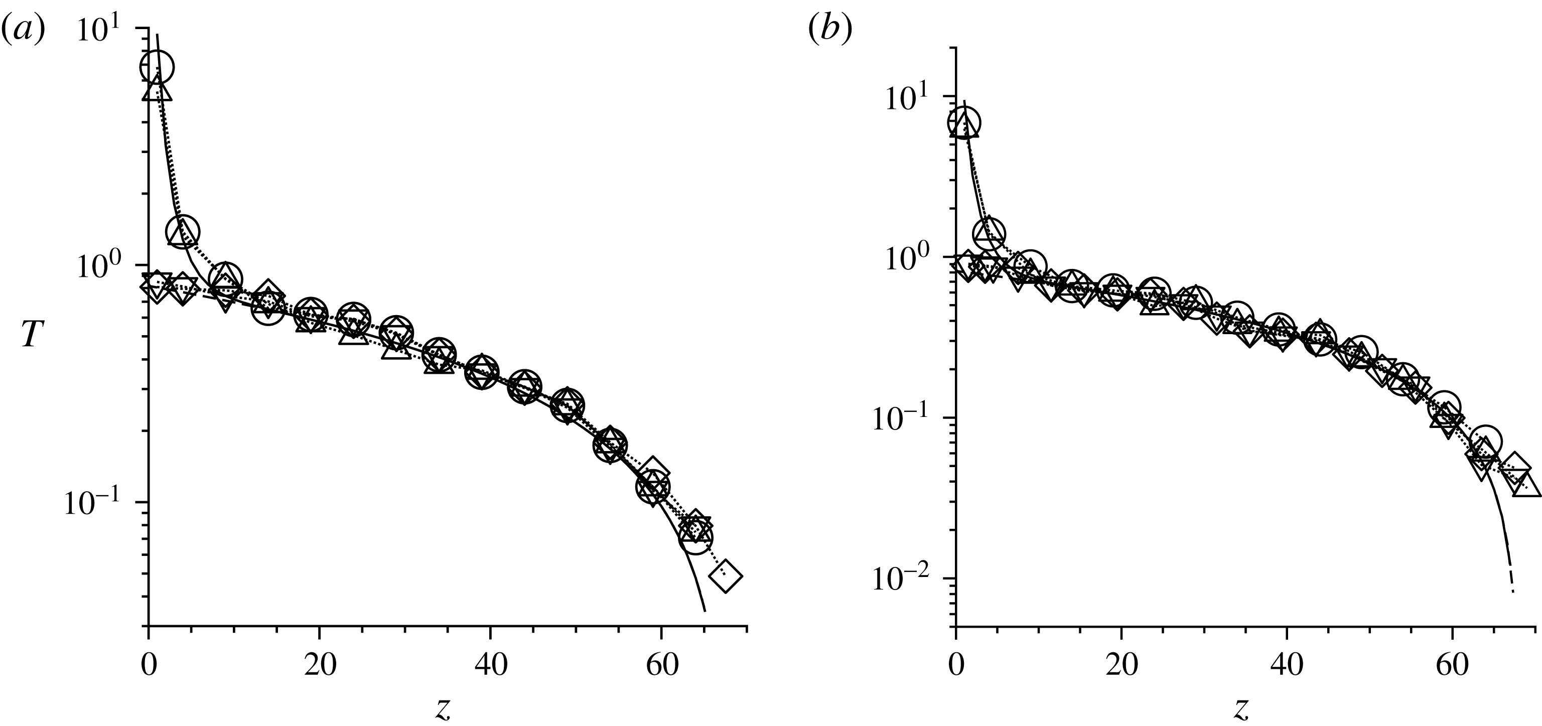
Figure 10 shows that there is a dramatic increase in the temperature at the base for sinusoidal bases, but there is no increase in temperature for frozen-particle bases. Consistency requires that the temperature and strain rate profiles in both cases should approach the same value in the flat-base limit; that is, zero amplitude for sinusoidal bases and zero base particle diameter for frozen-particle bases. The simulations show that the temperature profiles are independent of the base amplitude for sinusoidal bases, and the disordered energetic basal layer is observed even for a flat base. In contrast, for the frozen-particle base, the temperature at the base increases as the base particle diameter is decreased. This is shown in figure 12, where the temperatures for random and hexagonally ordered frozen-particle bases are shown as a function of the base particle diameter. For the random frozen-particle base, it is observed that the base is dissipative when the base particle diameter is decreased from 0.56 to 0.20. However, when the base particle diameter is decreased from 0.20 to 0.15, there is an abrupt change in the temperature profiles from a dissipative base to an energetic base. Further decrease in the base particle diameter does not alter the temperature profile. The strain rate profiles, not shown here, also exhibit a similar behaviour. In § 3.5, it is shown that the dissipative/energetic nature of the base also coincides with the absence/presence of a slip velocity and high angular velocity at the base.
The temperature profiles for the ordered flow over a random frozen-particle base (a) and an ordered frozen-particle base (b) for flowing layers with a height of approximately 70 flowing particle diameters using the linear contact model. In (a), profiles are shown for base particle diameters of 0.15 (▵), 0.20 (▿) and 0.56 (♢), and in (b), for base particle diameters of 0.50 (▵), 0.60 (▿) and 1.34 (♢). In all cases, (○) shows the results for a smooth base. The solid line is the best fit for the temperature from (2.24).

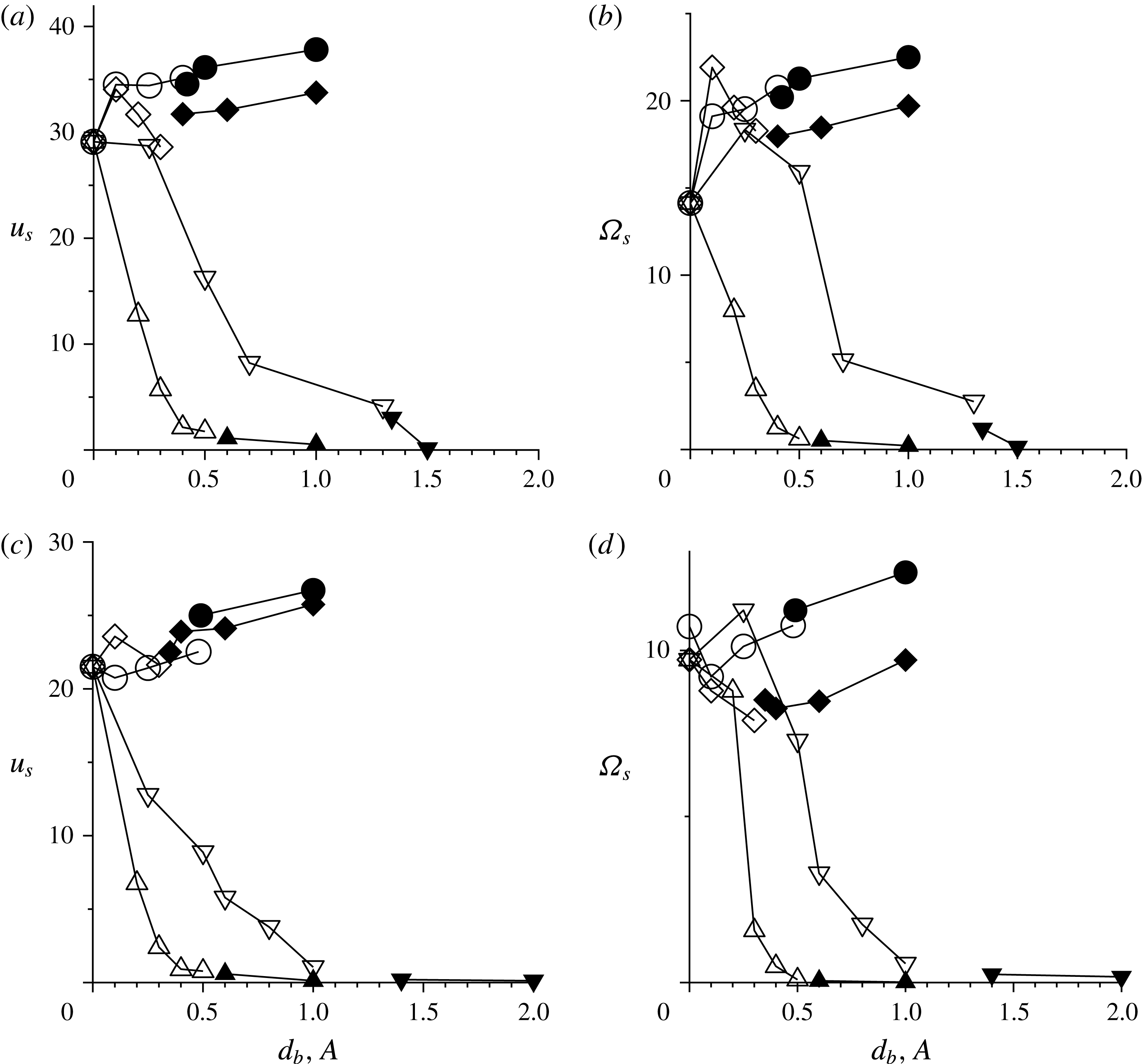
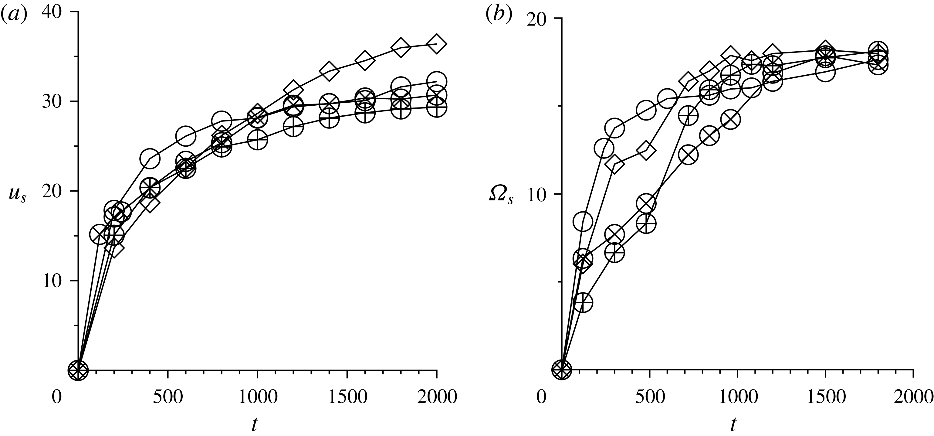
The slip velocity at the base (a,c) and the mean angular velocity of the particles with centres within one particle diameter of the base (b,d) as a function of the base particle diameter
 $d_{b}$
for frozen-particle bases or base amplitude
 $A$
for sinusoidal bases for (○) streamwise sinusoidal modulation with wavelength
 $40$
, (♢) spanwise sinusoidal modulation with wavelength
 $10$
, (▵) random frozen-particle base and (▿) hexagonally ordered frozen-particle base for a flowing layer of height approximately 70 particle diameters (a,b) and approximately 35 particle diameters (c,d) using the linear contact model.

3.5 Slip velocity
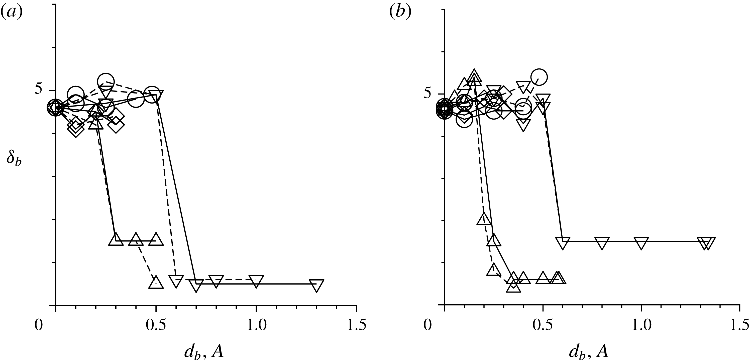
The slip velocity
 $u_{s}$
and the mean angular velocity
 $\unicode[STIX]{x1D6FA}_{s}$
of the particles with centres within a distance of 1 particle diameter from the base are shown as a function of the base roughness in figure 13. The slip velocity is shown in figure 13(a) for a layer height of approximately 70 particle diameters and in figure 13(c) for a layer height of approximately 35 particle diameters. The slip velocity is relatively large for sinusoidal bases, and it shows no systematic variation with base amplitude, wavelength, direction of modulation or particle contact model. The slip velocity does increase as the layer height is increased from approximately 35 to approximately 70 particle diameters, but this increase is sublinear with height. The slip velocity for frozen-particle bases is close to zero when the base particle diameter is large for both ordered and disordered flows. As the base particle diameter decreases, there is a sharp increase in the slip velocity at an amplitude of less than approximately
 $0.2$
for random bases and approximately
 $0.5$
for hexagonally ordered bases. As the base particle diameter is further decreased, the slip velocity tends to a constant value at zero amplitude. As required by consistency, in the limit of zero roughness, the slip velocity is the same for sinusoidal and frozen-particle bases. Figures 13(b) and 13(d) show the mean angular velocity of the particles closest to the base as a function of roughness for layers of height approximately 70 and 35 particle diameters respectively. The similarity in the qualitative variation of
 $u_{s}$
and
 $\unicode[STIX]{x1D6FA}_{s}$
is striking, indicating that the slip at the base and the particle rotation rate of the layer closest to the base are strongly correlated. This correlation is not because the particles closest to the base roll on the surface without sliding. If the particles were to roll on the bottom surface, the slip velocity and the angular velocity would satisfy the relation
 $u_{s}=(\unicode[STIX]{x1D6FA}_{s}d/2)$
; this relationship is clearly not satisfied because the slip velocity is a factor of
 $2$
larger than
 $\unicode[STIX]{x1D6FA}_{s}d$
.
The thickness of the basal disordered layer for the linear contact model (a) and the Hertzian contact model (b) as a function of the base particle diameter
 $d_{b}$
for frozen-particle bases or base amplitude
 $A$
for sinusoidal bases for (○) streamwise sinusoidal modulation with wavelength
 $40$
, (♢) spanwise sinusoidal modulation with wavelength
 $10$
, (▵) random frozen-particle base and (▿) hexagonally ordered frozen-particle base for a flowing layer of height approximately 35 particle diameters (dashed line) and approximately 70 particle diameters (solid line).

The
 $q_{6}$
order parameter (○), the number density
 $(n/6)$
(solid line), both referenced to the left vertical axis, and the mean velocity (dashed line), referenced to the right vertical axis, for the developing flow down an inclined plane using the Hertzian contact model over a sinusoidal base of wavelength
 $40$
in the streamwise
 $x$
direction and height
 $0.48$
at times
 $t=100$
(a),
 $t=200$
(b),
 $t=300$
(c) and
 $t=400$
(d).

Figure 14 shows the basal disordered layer thickness for the ordered flow. The variation of the height of the bottom disordered layer is qualitatively similar to those for the slip velocity and the mean angular velocity at the base. The height of the disordered layer shows no systematic variation with amplitude, wavelength or direction of modulation for sinusoidal bases. The height of the disordered layer is close to zero when the base particle diameter is relatively large for frozen-particle bases, but it shows a sharp increase as the base particle diameter is decreased below approximately 0.2 for the random frozen-particle base and approximately 0.6 for the ordered frozen-particle base. The disordered layer thickness tends to the same value as that for the sinusoidal base as the roughness amplitude tends to zero. Results for the two different flow heights considered here indicate that the slip velocity does increase with height, but the height of the disordered layer at the base does not depend on height. The thickness of this disordered layer, which is approximately 4–5 particle diameters, is also approximately the same as the best fit for the temperature boundary layer thickness
 $\unicode[STIX]{x1D6FF}$
in (2.24) for the temperature profiles in figure 10.
3.6 Flow development
The previous study of Kumaran & Bharathraj (Reference Kumaran and Bharathraj2013) showed that during the development of an ordered flow from an initially static and disordered assembly, there is an ordered shearing region at the bottom supporting a plug flow of particles in a random configuration above. The height of the ordered region increases linearly with time until it encompasses the entire layer, after which there is a further increase in the flow velocity until steady state is reached. The upward velocity of the ordering front was found to be independent of the flow height and the contact model, and was found to be approximately one particle diameter for every 13.5 time units for an angle of inclination of
 $22^{\circ }$
. The development of the ordered flow over a sinusoidal base is found to be the same as that above a frozen-particle base, as shown in figure 15. Here, the hexagonal order parameter
 $q_{6}$
and the number density profiles (scaled by a factor of 6 to fit within the same range as
 $q_{6}$
) are plotted on the left vertical axis, and the mean velocity profiles are shown by the dashed lines referred to the right vertical axis. Ordering and layering proceed simultaneously from the bottom to the top, with the upward propagation of an ordering front. There is shearing in the ordered region below, while the disordered plug above has a constant velocity. As indicated in Kumaran & Bharathraj (Reference Kumaran and Bharathraj2013), in the earliest stages of crystallisation at the base, there can be a variable time lag of approximately 50–100 time units due to the stochastic nature of the start of crystallisation. Apart from this, the qualitative and quantitative features of the ordering process are independent of the base topography, layer height or contact model.
There is also the growth of the disordered basal layer at the bottom, and the increase in the slip velocity at the base following the passage of the ordering front. Figure 15(a–d) shows that the region near the base first orders at early times, and then disorder from the base propagates upward. The slip velocity and the base temperature also increase with time. This disordered region at the bottom is not observed for ordered flows over frozen-particle bases.
The height of the ordering front,
 $\unicode[STIX]{x1D6FF}_{q6}$
, is shown as a function of time in figure 16(a). Here,
 $\unicode[STIX]{x1D6FF}_{q6}$
is defined as the height at which the
 $q_{6}$
order parameter (shown at different times in figure 15) is equal to
 $0.5$
. In this figure, the parameters for all symbols are as shown in table 1, except those for the ordered and random frozen-particle bases, where the base particle diameters are
 $0.50$
and
 $0.15$
respectively. In § 3.3, simulation results were reported to show that there is a disordered region of thickness approximately 5 particle diameters only when the base particle diameter is less than 0.60 and 0.20 for ordered and random frozen-particle bases; when the base particle diameter exceeds this critical value, there is no disordered region at the bottom. For a fair comparison, the base particle diameters shown in figure 16(b) are in the range where a disordered basal layer is observed in the simulations. The ordering front propagates at a constant velocity until it reaches the top of the layer. The upward velocity of the ordering front, which is approximately 1 particle diameter in every 13.5 time units (reported in Kumaran & Bharathraj (Reference Kumaran and Bharathraj2013)), is independent of the base topography and the layer height. Even though figure 16 is restricted to the Hertzian contact model, we have also verified that the velocity of the ordering front is independent of the contact model, and this appears to be a universal constant.
Figure 16(b) shows the upward progression of the disordered region at the bottom. Since the disordered region is only a few particle diameters in height and the order parameter cannot be resolved to within a particle diameter, the progress of the disordered layer at the bottom appears to be discontinuous, with larger variability in the exact location. However, it is apparent that the bottom disordered region also progresses upward due to the disruption of ordered layers that are already formed. The time scale for the disruption is a little larger than that for ordering. The final height of the disordered region is approximately 4–6 particle diameters in all cases.
The height of the ordered region (a) and the bottom disordered region (b) as a function of time for the ordered flow down an inclined plane of a layer of height approximately 70 particle diameters using the Hertzian contact model. The symbol descriptions are given in table 1, with the exception of the random and ordered frozen-particle bases, for which the base particle diameters are 0.15 (▵) and 0.50 (◃) respectively.

A distinct region at the base cannot be distinguished for a disordered flow. However, the temperature profiles in figure 10 do reveal a sharp increase in temperature at the base for sinusoidal bases, and significant velocity slip is observed in figure 7. The developing velocity profiles are shown as a function of time for the ordered and disordered flows over a sinusoidal base with modulation in the streamwise direction in figure 17. The nature of the flow development is very different for ordered and disordered flows. As shown in figure 15, there is an ordered shearing region at the bottom supporting a plug flow on top with no internal shearing. The front between these two distinct regions moves upwards at constant velocity until it reaches the top. This is also reflected in the velocity profiles in figure 17(a). In addition, there is also a continuous increase in the slip velocity at the base as the ordering front moves upwards. Even after the ordering front has reached the top, there is a further increase in the mean velocity and the slip velocity. For the disordered flow, the strain rate in the bulk during flow development is much smaller than that in the ordered flow, as shown in figure 17(b).
The velocity profiles during flow development over an inclined plane using the Hertzian contact model over a sinusoidal base with modulation in the streamwise direction with a base amplitude of 0.48 (a) and 0.49 (b) for a flow height of approximately 35 base particle diameters, at times 40 (○), 120 (▵), 300 (▿), 500 (◃) and 800 (♢) dimensionless time units since the start of flow.

The slip velocity at the base (a) and the angular velocity of particles within a height of 1 particle diameter from the base (b) as a function of time during flow development for a flowing layer over sinusoidal bases with a height of approximately 70 particle diameters using the Hertzian contact model. The parameters for the different symbols are given in table 1.

The increase in the slip velocity with time for both ordered and disordered flows over sinusoidal bases is shown in figure 18. The time scale for the development of the slip velocity is approximately the same for ordered and disordered flows, although the final steady-state values of the slip velocity do depend on the base topography and roughness. There is also a close correspondence in the increase in the average particle angular velocity within a region of 1 particle diameter at the base, shown in figure 18(b), and the increase in the slip velocity, indicating that the two are correlated. The mean angular velocity, which is zero initially, increases and reaches a steady value in the long-time limit. The time scales for the development of the slip velocity and the particle spin at the base are the same.
4 Conclusions
The present study is restricted to the flow of monodisperse spherical particles down an inclined plane. The particle interactions are modelled using the linear and the Hertzian spring–dashpot models, and periodic boundary conditions are employed in the streamwise and spanwise directions. Despite the idealised particle models, the results reveal several universal phenomena, such as transition and the bulk rheology in the ordered and disordered flows, as well as phenomena such as slip, base mobilisation and particle spin at the base, which depend on the base topography in non-obvious ways.
4.1 Transition
The discontinuous transition from an ordered to a disordered flow upon increasing the base roughness is found to be a universal phenomenon, independent of the type of base topography. The definition of base ‘roughness’ is topography-dependent, and is defined as the base particle diameter for frozen-particle bases and as the amplitude of the base modulation for sinusoidal bases. Regardless of the definition of the base roughness, we observe a transition from an ordered to a disordered flow at a critical value of the base roughness. The transition takes place when the base roughness is changed by less than 1 % of the moving particle diameter.
The characteristics of the flow in the bulk are independent of the base topography, but the characteristics of the ordered and disordered flows are very different. The ordered flow consists of distinct layers of particles sliding past each other, and there is hexagonally close-packed ordering of particles within the layers. In the disordered flow, there is no layering or in-plane ordering. The volume fraction in the ordered flow is actually higher than that in the disordered flow, and can be higher than the random close packing volume fraction. In the bulk, the structural properties of the ordered and disordered flows are independent of the base topography.
The transition roughness does depend on the type of base topography. The transition base particle diameter is less than the flowing particle diameter for random frozen-particle bases. Even when the base consists of ordered and hexagonally close-packed frozen particles, there is a transition from an ordered to a disordered flow when the base particle diameter exceeds approximately 1.35 times the flowing particle diameter. The critical base particle diameter does not depend on the angle of inclination or the contact model used, and shows very little dependence on the flow height. There is a transition for both streamwise and spanwise sinusoidal bases when the base amplitude exceeds a critical value. This critical base amplitude does depend on the flow height, the wavelength and the direction (streamwise or spanwise) of the base modulation. The critical base amplitude is independent of the angle of inclination or the particle contact model. The critical amplitude first increases and then decreases as the wavelength of the base modulation is increased. In the limit of low wavelength, the critical amplitude increases linearly with the wavelength and is independent of the flow height. When the wavelength is long compared with the height of the flowing layer, the critical amplitude decreases as
 $(1/\unicode[STIX]{x1D706})^{2}$
, or is proportional to the square of the wavenumber. The critical amplitude also appears to increase linearly with the flow height in the long-wavelength limit.
The present transition resembles two types of transition that have been observed in hard-particle systems, the crystallisation transition from a random configuration to a face-centred cubic crystal in an assembly of hard spheres at equilibrium (Alder & Wainwright Reference Alder and Wainwright1957; Young & Alder Reference Young and Alder1974) and the transition in a sheared hard-sphere system where particles form layers perpendicular to the flow direction which slide over each other (Erpenbeck Reference Erpenbeck1984). The hard-sphere crystallisation transition occurs in an equilibrium assembly of spherical particles, and it has been predicted by methods from kinetic theory (Kirkpatrick et al. Reference Kirkpatrick, Das, Ernst and Piasecki1990). The ordering in a sheared fluid of hard particles has also been examined using nonlinear fluctuating hydrodynamics about a non-equilibrium steady state (Lutsko, Dufty & Das Reference Lutsko, Dufty and Das1989; Lutsko Reference Lutsko2004). The present transition is different from the hard-sphere crystallisation or ordering transitions in that the granular flow is a driven dissipative system, far from equilibrium with no thermal noise. The transition is induced by modifications in the base roughness, that is, boundary effects, in contrast to the other hard-sphere transitions which are induced by changes in either the volume fraction or the shear rate. Moreover, the volume fraction and the shear rate are both self-selected in the present system, by the forces exerted parallel and perpendicular to the base.
Another important difference is that the flow height also affects the nature of the transition for sinusoidal bases. In the long-wave limit, the transition amplitude scales as the flow height and as the square of the wavenumber. This is different from the shear-induced transition in molecular hard-sphere systems, where the only length scale is the particle diameter, and transition is only a function of the shear rate once all lengths are scaled by the particle diameter (Lutsko et al. Reference Lutsko, Dufty and Das1989).
The scaling of the transition amplitude with wavelength in the limit of small wavelength is expected, since the wavelength is the only length scale in the problem. The scaling in the long-wave limit is intriguing. One possible explanation is based on the dilational instability discussed in Kumaran & Maheshwari (Reference Kumaran and Maheshwari2012), where an analogy was made between the layered flow and the layering in a lamellar liquid crystalline medium at equilibrium. When the system is dilated, so that the spacing between layers is higher than the equilibrium spacing, the layers bend so that the equilibrium spacing is restored. If a shear is applied on top of the dilation, the layers tend to buckle, and the layered state breaks. This explanation, borrowed from the dynamics of lamellar phases, recovers the correct scaling for the transition amplitude as a function of layer height if a small modification is made to the formulation of Kumaran & Maheshwari (Reference Kumaran and Maheshwari2012).
We consider a two-dimensional layered system with the
 $x$
axis along the layers and the
 $z$
axis perpendicular to the layers. The displacement field
 $u$
is defined as the displacement of the particles centres from the layer centre due to imposed perturbations, such as a rough base. The restoring force
 $f$
due to perturbations in the
 $z$
direction is found to be of the form
 $$\begin{eqnarray}f=B\frac{\unicode[STIX]{x2202}^{2}u}{\unicode[STIX]{x2202}z^{2}}-\frac{B}{2}\frac{\unicode[STIX]{x2202}}{\unicode[STIX]{x2202}z}\left(\frac{\unicode[STIX]{x2202}u}{\unicode[STIX]{x2202}x}\right)^{2}-B\frac{\unicode[STIX]{x2202}}{\unicode[STIX]{x2202}x}\left(\frac{\unicode[STIX]{x2202}u}{\unicode[STIX]{x2202}x}\frac{\unicode[STIX]{x2202}u}{\unicode[STIX]{x2202}z}\right)+\frac{B}{2}\frac{\unicode[STIX]{x2202}}{\unicode[STIX]{x2202}x}\left(\frac{\unicode[STIX]{x2202}u}{\unicode[STIX]{x2202}x}\right)^{3},\end{eqnarray}$$
where
 $B$
is the compression modulus. The first term on the right-hand side provides the linear approximation for the restoring force, while the other two terms are nonlinear terms required to render the strain rotation frame invariant. An additional term,
 $K(\unicode[STIX]{x2202}^{2}u/\unicode[STIX]{x2202}x^{2})$
, was added to the restoring force in Kumaran & Maheshwari (Reference Kumaran and Maheshwari2012); this term represents the surface tension in a fluid in which there is an energy penalty for increase in the surface area. This provides a scaling for the amplitude that is independent of the wavelength, as shown in Kumaran & Maheshwari (Reference Kumaran and Maheshwari2012). Here, instead of the surface tension term, we add a term that imposes a penalty for layer bending,
 $$\begin{eqnarray}f=B\frac{\unicode[STIX]{x2202}^{2}u}{\unicode[STIX]{x2202}z^{2}}-\frac{B}{2}\frac{\unicode[STIX]{x2202}}{\unicode[STIX]{x2202}z}\left(\frac{\unicode[STIX]{x2202}u}{\unicode[STIX]{x2202}x}\right)^{2}-B\frac{\unicode[STIX]{x2202}}{\unicode[STIX]{x2202}x}\left(\frac{\unicode[STIX]{x2202}u}{\unicode[STIX]{x2202}x}\frac{\unicode[STIX]{x2202}u}{\unicode[STIX]{x2202}z}\right)+\frac{B}{2}\frac{\unicode[STIX]{x2202}}{\unicode[STIX]{x2202}x}\left(\frac{\unicode[STIX]{x2202}u}{\unicode[STIX]{x2202}x}\right)^{3}-K\frac{\unicode[STIX]{x2202}^{4}u}{\unicode[STIX]{x2202}x^{4}},\end{eqnarray}$$
where
 $K$
is the bending modulus. In lamellar liquid crystalline media, the ratio
 $(K/B)=l^{2}$
, where
 $l$
is the layer spacing.
As in Kumaran & Maheshwari (Reference Kumaran and Maheshwari2012), if we impose a dilation on the system
 ${\mathcal{D}}$
, and periodic perturbations in the form of Fourier modes in the
 $x$
and
 $z$
directions,
 $$\begin{eqnarray}u={\mathcal{D}}z+\tilde{u} (t)\exp (\imath k_{x}x+\imath k_{z}z),\end{eqnarray}$$
the linear approximation for the restoring force is
 $$\begin{eqnarray}\tilde{f}=\left(-Bk_{z}^{2}+B{\mathcal{D}}k_{x}^{2}-Kk_{x}^{4}\right)\tilde{u} .\end{eqnarray}$$
The layered state becomes unstable when the direction of
 $\tilde{f}$
is along the direction of
 $\tilde{u}$
, so that a displacement fluctuation increases exponentially with time. If the dilation in the
 $z$
direction is homogeneous (
 $k_{z}=0$
), the condition for an instability is
 $$\begin{eqnarray}{\mathcal{D}}_{t}>(Kk_{x}^{2}/B),\end{eqnarray}$$
where
 ${\mathcal{D}}_{t}$
is the transition dilation. If the transition dilation is interpreted as the ratio of the transition amplitude
 $A_{t}$
and the layer height
 $h$
, the scaling for the transition amplitude is
 $$\begin{eqnarray}\frac{A_{t}}{h}\propto k_{x}^{2},\end{eqnarray}$$
where the wavenumber
 $k_{x}$
is the inverse of the wavelength. Equation (4.6) is the scaling observed in the present simulations. It is important to note that the scaling in (4.6) is not valid when the wavelength
 $(2\unicode[STIX]{x03C0}/k_{x})$
is comparable to the particle diameter or the layer spacing, and it is valid only when the wavelength is large compared with the particle diameter.
Thus, the scaling for the transition amplitude is predicted by an analysis for the dilational instability of layered flows, first proposed by Kumaran & Maheshwari (Reference Kumaran and Maheshwari2012), with the minor modification that the restoring force is due to layer bending instead of surface tension. However, a great deal more work needs to be carried out for a detailed understanding of the instability mechanism.
4.2 Bulk rheology and boundary layer thickness
For both the ordered and the disordered flows, the rheology in the bulk of the flow, for heights greater than approximately 10 particle diameters, is independent of the base topography. The bulk rheology is also independent of the flow height, although it does depend on the volume fraction.
For both ordered and disordered flows, it is observed that all of the components of the stress are proportional to the square of the strain rate. This is expected for hard-particle flows, where there is no material time scale and the only time scale is the inverse of the strain rate. However, the Bagnold coefficient (the ratio of the stress and the square of the strain rate) for a disordered flow is approximately one order of magnitude higher in comparison with that for an ordered flow. The angular velocity in the bulk is equal to one-half of the vorticity, indicating that the local particle rotation rates and material rotation rates are the same. In the context of kinetic models of dense flows down inclined planes, we also find that the ratio of the granular temperature and the square of the strain rate is a constant independent of the height within the bulk. Interestingly, this ratio is higher for a disordered flow in comparison with an ordered flow. This confirms that the assumption of instantaneous collisions made in kinetic theory based models is valid for both ordered and disordered flows.
The values of the parameters
 $p_{\unicode[STIX]{x1D719}}$
,
 $\unicode[STIX]{x1D707}_{\unicode[STIX]{x1D719}}$
and
 $D_{\unicode[STIX]{x1D719}}$
in the kinetic equations (2.20) can now be determined from the angle of inclination, the slope of the temperature profile in figure 10 and the ratio
 $(T/(\text{d}u_{x}/\text{d}z)^{2})$
in figure 11. These parameters are shown for the different models in table 2. The kinetic parameters do depend on the contact model used. It is clear that the kinetic parameters are independent of height for the linear contact model. This is because the coefficient of restitution in a particle collision is independent of the precollisional velocity in the linear model, and the volume fraction is a constant independent of height. The kinetic parameters do depend on height in the Hertzian contact model, and they seem to increase as the height increases. This is because the coefficient of restitution is velocity-dependent for the Hertzian model; the dissipation coefficient, in particular, increases as the relative velocity increases. Since higher flowing layers have a higher average temperature, the rate of dissipation of energy is also higher. This results in a height dependence of the kinetic parameters and the Bagnold coefficients. There is also a significant difference in the kinetic parameters for ordered and disordered flows. The dissipation parameter
 $D_{\unicode[STIX]{x1D719}}$
for a disordered flow is 3–5 times higher than that for an ordered flow, while the parameters
 $p_{\unicode[STIX]{x1D719}}$
and
 $\unicode[STIX]{x1D707}_{\unicode[STIX]{x1D719}}$
are one order of magnitude higher for disordered flows in comparison with ordered flows. Surprisingly, this and previous studies have shown that the Bagnold law is still a good approximation in the bulk even for a Hertzian model, despite the difference in the temperature dependence of the energy dissipation rate.
The kinetic parameters
 $p_{\unicode[STIX]{x1D719}}$
,
 $\unicode[STIX]{x1D707}_{\unicode[STIX]{x1D719}}$
and
 $D_{\unicode[STIX]{x1D719}}$
in (2.20), determined from the best fits for the slope of the temperature in the bulk in figure 10 and the ratio
 $(T/(\text{d}u_{x}/\text{d}z)^{2})$
in figure 11.
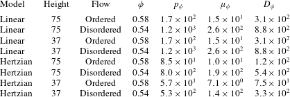
An analysis of the temperature profiles in figure 10 shows that the expression (2.24) from thermal boundary theory does predict the temperature at the base of the flow. The two parameters, the thermal boundary layer thickness
 $\unicode[STIX]{x1D6FF}$
and the constant
 $c$
, which is related to the energy input from the boundary, were calculated for the different base topographies considered here. It was found that the thermal boundary layer thickness
 $\unicode[STIX]{x1D6FF}$
depends only on the type of flow (ordered or disordered) and is independent of the base topography and the flow height. The constant
 $c$
, which is evaluated from the inverse of the slip length
 $\unicode[STIX]{x1D6FD}$
in the boundary condition at the base (boundary condition (2.25)), does depend on the base topography. In fact, we find a stronger restriction that the thermal boundary layer thickness is independent of the nature of contacts (linear or Hertzian) as well; the same thermal boundary layer thickness appears to fit the temperature profiles for both the linear and the Hertzian models. Thus, the thermal boundary layer thickness appears to attain a constant value in the hard-particle limit, independent of the type of contact model used. This is in accordance with the predictions of the thermal boundary layer theory that the boundary layer thickness can be derived only from the parameters in the viscometric relations for a hard-particle system.
4.3 Base topography
The effect of the base topography is restricted to a region of height 5–10 particle diameters at the base, but there are significant and counterintuitive changes in the flow within this basal layer as the base topography is changed. For flows over sinusoidal bases with large slip velocities, there are two distinct basal layers, the smaller spin boundary layer involving angular velocity disequilibrium and the larger temperature boundary layer involving energy disequilibrium. The particle spin is significantly higher than the material rotation rate in the spin boundary layer of thickness approximately 1 particle diameter, and it is comparable to the ratio of the slip velocity and the particle diameter. When the height is greater than approximately 2 particle diameters, the particle angular velocity equilibrates to the material rotation rate. There is a temperature boundary layer of height approximately 10 particle diameters where the rate of energy conduction is comparable to the rates of production and dissipation. Here, the granular temperature is an order of magnitude higher than that in the bulk. The above features of the flow over sinusoidal bases are common to ordered and disordered flows. For ordered flows, disruption of ordering is also observed within the temperature boundary layer, and there is a region of height approximately 5 particle diameters where the particle configuration is random.
The physical picture for sinusoidal bases is that the spin boundary layer consisting of rapidly spinning particles enables slip at the base, and also acts as a source of particle fluctuating energy. The energy generated is conducted through the temperature boundary layer, resulting in large particle agitation and mobility. Due to their roughness, frozen-particle bases appear to disrupt the buildup of angular velocity at the base. The spin boundary layer is absent for flows over frozen-particle bases, and so there is angular velocity equilibrium down to the base, and the temperature and strain rate at the base are comparable to those in the bulk.
A consistency requirement is that the properties of the basal layer tend to those for a flat base when the base roughness decreases to zero. We find that there is little change in the slip velocity and the thickness of the basal layer for sinusoidal bases when the base amplitude is decreased to zero. However, there is a significant change in the basal layer for frozen-particle random and ordered bases as the base particle diameter decreases to zero. In the latter case, when the base particle diameter is greater than a threshold of approximately 20 % and 60 % of the moving particle diameter for random and ordered frozen-particle bases respectively, there is no discernible disordered basal layer and the slip velocity is small. When the base particle diameter decreases below this threshold, there is a systematic increase in the slip velocity, the basal angular velocity and the thickness of the disordered layer at the base, and the smooth wall characteristics are approached as the base particle diameter decreases to zero. Thus, the properties of the basal layer are independent of the amplitude and wavelength for sinusoidal bases, but they do undergo a transition from the ordered low-temperature no-slip flow to the disordered highly energetic slip flow as the base particle diameter is decreased for frozen-particle bases.
4.4 Flow development
In an ordered flow, when a static layer of randomly arranged particles is inclined, ordering progresses from the bottom to the top. At intermediate times, there is an ordered and shearing layer of particles at the bottom supporting a disordered layer of particles above moving at constant velocity with no internal shearing. The ordering front moves upwards until it reaches the top surface and the entire flow is ordered; there is a further increase in the flow velocity after complete ordering until steady state is attained. The front propagates upward at a velocity that is a constant independent of the particle contact model, the nature of the base roughness or the height of the layer. For sinusoidal and flat bases, where there is a disordered and highly fluidised layer of particles at the bottom, the slip velocity develops at approximately the same rate as the progress of the ordering front. The disordered layer at the bottom also develops by the upward progression of a ‘disorder front’ after the bottom layers have been ordered, and at approximately the same rate as the slip velocity. The time scale for the development of the slip velocity and the disordered bottom region shows no dependence on the base amplitude or direction of modulation. However, it should be cautioned that there is greater scatter in the data for the development of the slip velocity and the disordered region at the bottom.
4.5 Practical significance
Flows over inclined planes have hitherto been classified into three broad categories: flows over ‘bumpy bases’, where there is shearing throughout the height and there is no slip at the bottom, flows over ‘flat frictional’ bases, where there is a thin sliding layer at the bottom supporting a static pile on top, and flows over ‘erodible bases’, where the layer of particles supporting the flow is identical to the flowing particles. The ability of the flow in the bulk to sense the base configuration has been a source of confusion, since this contradicts the concept of local rheology. The resolution suggested by the present study is the presence of a highly fluidised layer of height approximately 10 particle diameters at the bottom for certain types of base topography with granular temperatures that are 1–2 orders of magnitude higher than that in the bulk, coupled with very high shear rates. The energy source is provided by a layer of thickness approximately 1 particle diameter with very high angular velocity, which also facilitates velocity slip at the bottom. While the shearing in the bulk is not affected by the base configuration, the relatively much larger slip velocity and shearing at the base would make it appear as though there is a static region supported by a highly energetic layer at the bottom. This could explain the dramatic differences in the characteristics of flows above flat frictional and bumpy bases.
The wide variation in the slip velocity with the base topography is also a candidate explanation for the wide disparities in the Froude number correlations for flows over inclined planes. For a Bagnold velocity profile with a no-slip condition at the bottom, the Froude number,
 $(\bar{u}/\sqrt{gh})$
, is expected to scale as
 $h$
, where
 $\bar{u}$
is the height-averaged velocity. Departure from this scaling relationship has been interpreted as evidence that the Bagnold law is not valid in the bulk of the flow. However, when interpreting data in this manner, it is important to consider the possibility of basal slip and an energetic basal layer for gentler base topographies, and the absence of the same for rougher base topographies. In the extreme case where the slip velocity at the base is much larger than the velocity variation in the bulk, the Froude number would be expected to scale as
 $h^{-1/2}$
. For real systems with basal slip, the Froude number scaling could vary between
 $h$
and
 $h^{-1/2}$
when the Bagnold rheology is valid in the bulk, due to the slip velocity at the base.
The reason for highly energetic basal layers for certain types of base topographies is counterintuitive. It would ordinarily be expected that the agitation at the base would be higher for rougher base topographies such as frozen-particle bases and lower for gentler topographies such as long-wavelength small-amplitude sinusoidal bases. Here, we find precisely the opposite, that gentler base topographies such as flat and sinusoidal bases generate temperatures that are one to two orders of magnitude greater than frozen-particle bases. The reason for this, uncovered in the present study, is a spin boundary layer for gentler topographies, which facilitates base slip and acts as a source of fluctuating energy. This spin boundary layer is not present for rough bases, resulting in no slip and lower particle agitation. An understanding of the causative mechanisms will facilitate better models for the effect of the base topography in geophysical flows, and opens up the intriguing possibility of tailoring the base topography to achieve specific flow characteristics in industrial applications.
Acknowledgement
The authors thank the Department of Science and Technology, Government of India for financial support. This research was supported by the J. R. D. Tata Trust.