1 Introduction
The prediction of laminar–turbulent transition is a key factor in the aero-thermal design of hypersonic vehicles. Transition has a dramatic effect on skin friction and heat transfer rates on the surface of a body flying at hypersonic speeds, and it is necessary to understand the physical mechanisms involved in order to be able to accurately predict the transition point. The main route from the laminar to turbulent state, in the case of small-amplitude environmental disturbances, can be summarised in the following three fundamental processes: (a) receptivity, (b) eigenmode growth of instabilities and (c) nonlinear breakdown to turbulence.
The whole process leading to breakdown depends on the initial conditions established by the receptivity mechanism. The receptivity process is, in turn, affected by parameters related to the flow conditions, such as the Mach and Reynolds numbers, and by the nature of the external environmental disturbances as well as local geometrical features such as nose bluntness, surface roughness and waviness. The natural receptivity, in particular, concerns the generation of boundary-layer disturbances by means of the environmental disturbance field, including acoustic, vorticity and entropy waves (Saric, Reed & Kerschen Reference Saric, Reed and Kerschen2002). For subsonic flows, the wavelengths and phase speeds of the external disturbances are in general much different to those of the internal modes, i.e. the external waves and the boundary-layer modes are de-synchronised (Nishioka & Morkovin Reference Nishioka and Morkovin1986). Hence, in this case a process of energy transfer from the wavelength of the forcing to that of the generated internal wave is needed. This wavelength-conversion mechanism, for a certain frequency, is promoted in regions of short-scale streamwise variations of the mean flow, including the leading edge, as well as regions with high curvature such as roughness and wall humps, as described by Goldstein & Hultgren (Reference Goldstein and Hultgren1989). At hypersonic Mach numbers, however, the small difference in phase speed between the forcing waves and the dominant boundary-layer modes can lead to a direct excitation of these modes via a resonance mechanism near the leading edge (Fedorov & Khokhlov Reference Fedorov and Khokhlov2001; Fedorov Reference Fedorov2003; Zhong & Ma Reference Zhong and Ma2006; Zhong & Wang Reference Zhong and Wang2012), without the need for a wavelength-conversion mechanism. This does not imply that in hypersonic flows a wavelength-conversion mechanism at the leading edge does not exist, but only that it is not needed for the generation of the internal boundary-layer modes, as it is essentially ‘bypassed’ by a resonance mechanism occurring near the leading edge. This resonance mechanism was introduced by Fedorov & Khokhlov (Reference Fedorov and Khokhlov2001), whose results refer to nominally zero-pressure-gradient flows, for example just past the leading edge, and describe the receptivity mechanism in the so-called ‘upstream’ region, i.e. the region preceding the excitation of the second instability mode.
According to the theoretical results of Fedorov & Khokhlov (Reference Fedorov and Khokhlov2001), receptivity at hypersonic speeds can be divided into two alternative processes based on either (a) the receptivity to fast acoustic or entropy or vorticity waves, or (b) the receptivity to slow acoustic waves. When the first class of waves interact with the boundary layer, a stable mode (the so-called fast mode, or mode F, according to the Fedorov (Reference Fedorov2003) notation) is generated at the leading edge by direct resonant interaction (or synchronisation) with the forcing waves. This mode, whose phase speed gradually decreases in the streamwise direction, is at first strongly excited in the early nose region, but then decays when it is no longer synchronised with the phase speed of the forcing waves. During its decay, the fast mode enters a modulation process with the external waves, as shown by Ma & Zhong (Reference Ma and Zhong2005), and, further downstream, leads to the excitation of a lower phase-speed boundary-layer instability mode (denoted as mode S, or slow mode, since its phase speed is close to the value of slow acoustic waves), belonging to the class of Mack modes (Mack Reference Mack1984). Among the higher-frequency Mack modes, the second mode was found to play a major role in the transition process of hypersonic boundary layers by Stetson et al. (Reference Stetson, Thompson, Donaldson and Siler1984). In this case, the excitation of the unstable mode (mode S) was initially due to a synchronisation process with the decaying fast mode (mode F). In the case of slow acoustic waves, in contrast, mode S can be directly generated at the leading edge through the resonance mechanism with the slow acoustic waves. The subsequent growth of instability modes is usually taken to be predictable using established tools such as the parabolised stability equations (PSE), as was demonstrated by Malik & Balakumar (Reference Malik and Balakumar2007) for a blunt flat plate at Mach number 3.5.
In the case of free-stream high-amplitude disturbances, nonlinearities can lead to a rapid transition to turbulence. In some conditions, transition occurs as a result of transient growth, whose related mechanism in hypersonic flows, similarly to what was found in low-speed flows (Andersson et al. Reference Andersson, Brandt, Bottaro and Henningson2001; Brandt & Henningson Reference Brandt and Henningson2002), is associated with the conversion of streamwise vorticity into streamwise streaks via a lift-up effect, as was shown by Paredes, Choudhari & Li (Reference Paredes, Choudhari and Li2016a), Paredes et al. (Reference Paredes, Choudhari, Li and Chang2016b,Reference Paredes, Choudhari, Li and Changc) for flat-plate and circular-cone flows at hypersonic Mach numbers. Another possibility is based on oblique transition (Berlin & Henningson Reference Berlin and Henningson1999), in which the response to oblique free-stream waves in combination with a nonlinear mechanism was found to be a powerful process, characterised by non-modal growth of the disturbances and requiring lower initial amplitudes compared to the case of transition caused by two-dimensional Tollmien–Schlichting (TS) and second mode instabilities.
Three-dimensional boundary layers, e.g. on swept wings or axisymmetric cones at an angle of incidence, can include additional instability modes, which are linked to inflectional cross-flow boundary-layer profiles. Boundary layers in the presence of cross-flow instabilities have been studied extensively in low-speed flows, e.g. in the works of Kohama (Reference Kohama1987), Reed & Saric (Reference Reed and Saric1989), Bippes (Reference Bippes1999) and White & Saric (Reference White and Saric2005). The final breakdown to turbulence is then caused further downstream by the development of high-frequency secondary instabilities of the deformed mean flow (Kohama Reference Kohama1987; Malik et al. Reference Malik, Li, Choudhari and Chang1999; White & Saric Reference White and Saric2005). Cross-flow instabilities include both stationary and travelling waves (Choudhari Reference Choudhari1994). The stationary modes are usually associated with surface roughness, whereas the travelling modes are linked to vortical free-stream disturbances and are expected to be dominant in noisy environments. Travelling cross-flow waves are usually found in a relatively low-frequency range. Borg, Kimmel & Stanfield (Reference Borg, Kimmel and Stanfield2015), for example, detected linearly growing travelling waves in quiet conditions, with a peak centred at 45 kHz, in their Mach 6 experiment over a scaled model of the Hypersonic International Research Experimentation Program’s Five (HIFiRE-5) elliptic cone in the Mach 6 Purdue quiet tunnel. In another experimental study at hypersonic conditions, Craig & Saric (Reference Craig and Saric2016) considered flow over a  $7^{\circ }$ right circular cone at
 $5.6^{\circ }$ angle of attack in the Mach 6 quiet tunnel at Texas A&M University. Consistent with the low-speed findings, they observed stationary vortices growing and significantly deforming the mean flow, and then attenuating after reaching nonlinear saturation. Moreover, they measured unsteady fluctuations in two different frequency bands of 15–60 kHz and 80–130 kHz. The disturbances in the lower-frequency band were attributed to growing travelling cross-flow waves, whereas those in the high-frequency band were identified as secondary instabilities. Similar results were obtained experimentally by Ward, Henderson & Schneider (Reference Ward, Henderson and Schneider2015) for a Mach 6 flow over a yawed circular cone. Again high-frequency secondary instability was identified as being the cause for the breakdown of the stationary vortices, but disturbances in a lower-frequency range of 40–50 kHz, were also detected as and associated with travelling cross-flow modes.
From a theoretical and simulation perspective, the works of Choudhari et al. (Reference Choudhari, Li, Chang, Carpenter, Streett, Malik and Duan2013), based on linear/nonlinear parabolised stability equations, and of Li et al. (Reference Li, Choudhari, Duan and Chang2014), based on secondary instability theory, PSE and direct numerical simulation (DNS) results, have shed light on the important role played by the growth of the secondary instabilities of primary travelling cross-flow waves, as a viable transition scenario when the initial amplitudes of the travelling waves are comparable to those of the stationary modes. The amplification characteristics of secondary instabilities originating from stationary cross-flow modes over a circular cone at moderate angle of incidence were investigated by Li et al. (Reference Li, Choudhari, Paredes and Duan2016) by quasi-parallel stability theory and PSE. In their computations, stationary vortices were excited to finite amplitudes by an azimuthally periodic array of roughness elements. Results showed that secondary instabilities may originate from different unstable modes, which were identified as strongly modulated travelling cross-flow waves (found in two different frequency bands with peak below 100 kHz, namely 14 kHz and 93 kHz), higher-frequency Mack modes, and secondary instabilities. Travelling waves and Mack modes are instabilities of the unperturbed flow, but are so strongly modulated by the presence of the stationary vortices that they lose their original characteristics and evolve downstream, effectively as secondary instabilities of the primary stationary modes.
Further stability calculations and direct numerical simulations of cross-flow instabilities have been carried out for swept wings, circular cones at an angle of attack and elliptic cones. Balakumar & Owens (Reference Balakumar and Owens2010) and Balakumar & King (Reference Balakumar and King2012) reported substantially higher amplification ( $N$) factors for travelling cross-flow waves compared to stationary waves in flows over a circular cone at
 $6^{\circ }$ angle of attack, a swept cylinder and a swept wing with sharp and blunt leading edge. DNS results of Bartkowicz, Subbareddy & Candler (Reference Bartkowicz, Subbareddy and Candler2010), for Mach 8 flow over the HIFiRE-5 elliptic cone model, showed the evolution of a system of streamwise vortices forming next to the centreline bulge at different Reynolds numbers, and associated these vortices with stationary cross-flow waves. The addition of acoustic noise caused unsteady waves to form on top of the vortices, causing their breakdown at the highest Reynolds numbers. More recent DNS simulations of Dinzl & Candler (Reference Dinzl and Candler2017) showed a difference between the centreline system of vortices and the cross-flow vortices generated by surface roughness. Recent studies based on biglobal linear stability analysis (Paredes & Theofilis Reference Paredes and Theofilis2015; Paredes et al. Reference Paredes, Gosse, Theofilis and Kimmel2016d) conducted on the HIFiRE-5 geometry confirmed the dominant role played by the cross-flow instabilities in the off-centreline region, as well as the presence of different instability modes occurring along the centreline bulge, as was first identified by Choudhari et al. (Reference Choudhari, Chang, Jentink, Li, Berger, Candler and Kimmel2009). These centreline modes can explain the strong disturbance growth observed in the computations of Bartkowicz et al. (Reference Bartkowicz, Subbareddy and Candler2010) along the centreline. Experiments (Juliano, Borg & Schneider Reference Juliano, Borg and Schneider2015) have confirmed the presence of both centreline and off-centreline transition in noisy conditions.
Previous work on cross-flow-induced transition in hypersonic boundary layers has often considered fully three-dimensional cases, in which it is difficult to separate out the fundamental aspects from those that are geometry specific, such as the centreline modes on elliptic cones. In the present contribution we consider a planar leading-edge geometry (a cylinder–wedge combination) in which, by definition, the base flow does not vary in the spanwise direction. We present DNS of the complete transition process in unswept and swept configurations. The simulations start from acoustic free-stream disturbance, which are known to be the dominant type of disturbance in hypersonic wind tunnels, as reported by previous experimental works (Schneider Reference Schneider2001, Reference Schneider2008, Reference Schneider2015; Masutti et al. Reference Masutti, Spinosa, Chazot and Carbonaro2012; Parziale, Shepherd & Hornung Reference Parziale, Shepherd and Hornung2014), and more recently confirmed by the numerical study of Duan, Choudhari & Wu (Reference Duan, Choudhari and Wu2014) and the combined experimental–numerical study of Wagner et al. (Reference Wagner, Schülein, Petervari, Hannemann, Ali, Cerminara and Sandham2018). Simulations are carried out for fast and slow acoustic disturbances as well as for two different amplitudes to identify key nonlinear aspects. Section 2 details the methodology. Section 3 shows the results for unswept cases, which at low amplitude confirm the receptivity mechanism and at high amplitudes show a streak-based breakdown process. Section 4 provides results and interpretation for the swept cases. Key findings of this section include the identification of a previously unseen breakdown scenario in the swept case that involves high wavenumber streamwise structures that serve to break down the flow faster than sinuous or varicose secondary instabilities of the primary cross-flow mode.
2 Methodology
2.1 Governing equations
We consider numerical solutions of the three-dimensional Navier–Stokes equations for compressible flows, written in conservation form, under the assumption of calorically perfect gas. The non-dimensional conservation equations in Cartesian coordinates can be written as
 $$\begin{eqnarray}\frac{\unicode[STIX]{x2202}\boldsymbol{Q}}{\unicode[STIX]{x2202}t}+\frac{\unicode[STIX]{x2202}\boldsymbol{F}_{j}}{\unicode[STIX]{x2202}x_{j}}=0,\end{eqnarray}$$
where  $\boldsymbol{Q}$ and
 $\boldsymbol{F}_{j}$ are vectors containing the conservative variables and the fluxes respectively, given by
 $$\begin{eqnarray}\displaystyle & \displaystyle \boldsymbol{Q}=\left[\begin{array}{@{}c@{}}\unicode[STIX]{x1D70C}\\ \unicode[STIX]{x1D70C}u\\ \unicode[STIX]{x1D70C}v\\ \unicode[STIX]{x1D70C}w\\ \unicode[STIX]{x1D70C}E\end{array}\right], & \displaystyle\end{eqnarray}$$
 $$\begin{eqnarray}\displaystyle & \displaystyle \boldsymbol{F}_{j}=\left[\begin{array}{@{}c@{}}\unicode[STIX]{x1D70C}u_{j}\\ \unicode[STIX]{x1D70C}uu_{j}+\unicode[STIX]{x1D6FF}_{1j}p-{\displaystyle \frac{1}{Re}}\unicode[STIX]{x1D70F}_{1j}\\ \unicode[STIX]{x1D70C}vu_{j}+\unicode[STIX]{x1D6FF}_{2j}p-{\displaystyle \frac{1}{Re}}\unicode[STIX]{x1D70F}_{2j}\\ \unicode[STIX]{x1D70C}wu_{j}+\unicode[STIX]{x1D6FF}_{3j}p-{\displaystyle \frac{1}{Re}}\unicode[STIX]{x1D70F}_{3j}\\ \unicode[STIX]{x1D70C}\left(E+{\displaystyle \frac{p}{\unicode[STIX]{x1D70C}}}\right)u_{j}-{\displaystyle \frac{1}{Re}}\left(u\unicode[STIX]{x1D70F}_{1j}+v\unicode[STIX]{x1D70F}_{2j}+w\unicode[STIX]{x1D70F}_{3j}+{\displaystyle \frac{\unicode[STIX]{x1D707}}{(\unicode[STIX]{x1D6FE}-1)PrM^{2}}}{\displaystyle \frac{\unicode[STIX]{x2202}T}{\unicode[STIX]{x2202}x_{j}}}\right)\end{array}\right]. & \displaystyle\end{eqnarray}$$
The velocity components ( $u$,
 $v$,
 $w$) are normalised by the free-stream main velocity (
 $U_{\infty }^{\ast }$), while the density (
 $\unicode[STIX]{x1D70C}$), temperature (
 $T$) and dynamic viscosity (
 $\unicode[STIX]{x1D707}$) are normalised by their corresponding free-stream values, namely
 $\unicode[STIX]{x1D70C}_{\infty }^{\ast }$,
 $T_{\infty }^{\ast }$,
 $\unicode[STIX]{x1D707}_{\infty }^{\ast }$ respectively. The normalisation factor used for the pressure (
 $p$) and viscous stresses (
 $\unicode[STIX]{x1D70F}_{ij}$) is
 $\unicode[STIX]{x1D70C}_{\infty }^{\ast }U_{\infty }^{\ast 2}$, whereas the free-stream kinetic energy per unit mass (
 $U_{\infty }^{\ast 2}$) is used to normalise the specific total energy (
 $E$). The characteristic length scale in the simulations is represented by the nose radius (
 $R^{\ast }$), with the Reynolds number defined as
 $Re=(\unicode[STIX]{x1D70C}_{\infty }^{\ast }U_{\infty }^{\ast }R^{\ast })/\unicode[STIX]{x1D707}_{\infty }^{\ast }$. The fluid-dynamic characteristic time is
 $R^{\ast }/U_{\infty }^{\ast }$. The Prandtl number is set to
 $Pr=0.72$, and the specific heat ratio is
 $\unicode[STIX]{x1D6FE}=1.4$.
The dynamic viscosity is, in turn, expressed in terms of temperature by Sutherland’s law
 $$\begin{eqnarray}\unicode[STIX]{x1D707}=T^{3/2}\frac{1+C}{T+C},\end{eqnarray}$$
where the constant  $C$ represents the ratio between Sutherland’s constant (set to 110.4 K) and the free-stream reference temperature (
 $T_{\infty }^{\ast }=51.7~\text{K}$). The viscous stresses are defined in terms of the velocity derivatives, under the assumption of a Newtonian fluid, as
 $$\begin{eqnarray}\unicode[STIX]{x1D70F}_{ij}=\unicode[STIX]{x1D707}\left[\frac{\unicode[STIX]{x2202}u_{i}}{\unicode[STIX]{x2202}x_{j}}+\frac{\unicode[STIX]{x2202}u_{j}}{\unicode[STIX]{x2202}x_{i}}-\frac{2}{3}\unicode[STIX]{x1D6FF}_{ij}\frac{\unicode[STIX]{x2202}u_{k}}{\unicode[STIX]{x2202}x_{k}}\right].\end{eqnarray}$$
We also need a relation linking the total energy (per unit mass) to the temperature, which in non-dimensional form can be expressed as
 $$\begin{eqnarray}E=\frac{T}{\unicode[STIX]{x1D6FE}(\unicode[STIX]{x1D6FE}-1)M^{2}}+\frac{1}{2}(u^{2}+v^{2}+w^{2}).\end{eqnarray}$$
Finally, the system of equations is closed by the dimensionless equation of state for a perfect gas
 $$\begin{eqnarray}p=\frac{1}{\unicode[STIX]{x1D6FE}M^{2}}\unicode[STIX]{x1D70C}T.\end{eqnarray}$$
The system of equations in Cartesian coordinates is transformed into a system of equations in curvilinear coordinates ( $\unicode[STIX]{x1D709}$,
 $\unicode[STIX]{x1D702}$,
 $\unicode[STIX]{x1D701}$) as
 $$\begin{eqnarray}\frac{\unicode[STIX]{x2202}\bar{\boldsymbol{Q}}}{\unicode[STIX]{x2202}t}+\frac{\unicode[STIX]{x2202}\bar{\boldsymbol{F}}_{j}}{\unicode[STIX]{x2202}\unicode[STIX]{x1D709}_{j}}=0.\end{eqnarray}$$
The relations between the vectors in curvilinear and Cartesian coordinates are expressed by
 $$\begin{eqnarray}\bar{\boldsymbol{Q}}=J\boldsymbol{Q},\quad \bar{\boldsymbol{F}}_{j}=J\boldsymbol{F}_{i}\frac{\unicode[STIX]{x2202}\unicode[STIX]{x1D709}_{j}}{\unicode[STIX]{x2202}x_{i}},\end{eqnarray}$$
with  $J=\det \Vert \unicode[STIX]{x2202}(x,y,z)/\unicode[STIX]{x2202}(\unicode[STIX]{x1D709},\unicode[STIX]{x1D702},\unicode[STIX]{x1D701})\Vert$ being the Jacobian of the transformation matrix.
2.2 Code features
The code we use to carry out our DNS computations is the SBLI (shock–boundary-layer interaction) code, developed over a number of years at the University of Southampton. In order to perform the computations for compressible flows in the presence of shock waves, the SBLI code uses a shock-capturing method, which is applied as a filter step to the solution obtained through the base scheme at the end of each time integration step. The base scheme is, in turn, based on a fourth-order central finite difference scheme for space discretisation, including the same-order boundary treatment (Carpenter, Nordström & Gottlieb Reference Carpenter, Nordström and Gottlieb1999) and makes use of an entropy-splitting method (Sandham, Li & Yee Reference Sandham, Li and Yee2002) to improve the nonlinear stability of the high-order central scheme. For time integration, a third-order Runge–Kutta scheme is used. The shock-capturing scheme consists of a second-order total variation diminishing (TVD)-type algorithm, with a particular compression method (Yee, Sandham & Djomehri Reference Yee, Sandham and Djomehri1999), which restricts the artificial dissipation to the shock region, thus providing minimum dissipation in the smooth regions. The scheme is supplemented with the Ducros sensor (Ducros et al. Reference Ducros, Ferrand, Nicoud, Weber, Darracq, Gacherieu and Poinsot1999), which turns off the artificial dissipation in vortical regions (i.e. the boundary layer). A favourable feature of this sensor is that it does not require any a priori knowledge of the shock position. The code works using MPI libraries, and has been set up to run in parallel, by dividing the domain into a number of sub-domains, and assigning each of them to a particular processor. Validations of the code can be found in the work of De Tullio et al. (Reference De Tullio, Paredes, Sandham and Theofilis2013), where DNS results are compared with PSE results for the case of transition induced by a discrete roughness element in a boundary layer at Mach 2.5, and in Cerminara (Reference Cerminara2017) for the specific case of hypersonic flow over blunt leading edges. The latter included a grid study based on the solution of the multi-frequency pressure fluctuation distribution along the wall for a Mach 6 flow between three grid levels. This study confirmed the suitability of the grid size used for the present problem.
2.3 Linear stability analysis
The linear stability analysis was performed using the NoSTRANA (non-local stability and transitional analysis) code by Sansica (Reference Sansica2015), whose validity was verified against the results of the reference work of Malik (Reference Malik1990). The code solves the linearised Navier–Stokes equations, based on a normal mode ansatz
 $$\begin{eqnarray}\boldsymbol{q}^{\prime }(x,y,z,t)=\hat{\boldsymbol{q}}(y)\boldsymbol{\cdot }\text{e}^{\text{i}(\unicode[STIX]{x1D6FC}x+\unicode[STIX]{x1D6FD}z-\unicode[STIX]{x1D714}t)},\end{eqnarray}$$
in which  $\hat{\boldsymbol{q}}(y)$ represents the eigenvector, containing the eigenfunctions
 $\hat{\unicode[STIX]{x1D70C}}(y)$,
 $\hat{u} (y)$,
 $\hat{v}(y)$,
 ${\hat{w}}(y)$ and
 $\hat{T}(y)$,
 $\unicode[STIX]{x1D6FC}$ is the streamwise wavenumber,
 $\unicode[STIX]{x1D6FD}$ the spanwise wavenumber and
 $\unicode[STIX]{x1D714}$ is the angular frequency. For local linear stability analysis, we define
 $y$ as the wall-normal direction and
 $z$ as the spanwise direction (parallel to the leading edge), with
 $x$ perpendicular to both of these. It should be noted that this is different to the coordinate system defined later for the DNS, but we prefer not to over-complicate the notation here. The linear system of partial differential equations reduces to a linear system of ordinary differential equations
 $$\begin{eqnarray}\unicode[STIX]{x1D647}\hat{\boldsymbol{q}}=\unicode[STIX]{x1D714}\unicode[STIX]{x1D646}\hat{\boldsymbol{q}},\end{eqnarray}$$
where  $\unicode[STIX]{x1D647}$ is a matrix containing the
 $y$-dependent coefficients of the system, the wavenumbers
 $\unicode[STIX]{x1D6FC}$,
 $\unicode[STIX]{x1D6FD}$ and the
 $y$-derivatives of the components of the variable vector
 $\hat{\boldsymbol{q}}$; while
 $\unicode[STIX]{x1D646}$ is a diagonal matrix containing the terms arising from the time derivative of the complex exponential function in (2.10). Sansica (Reference Sansica2015) derives all the components of the matrices
 $\unicode[STIX]{x1D647}$ and
 $\unicode[STIX]{x1D646}$ in the system of (2.11), and gives a description of the Chebyshev discretisation method. The solution of this eigensystem provides eigenvalues and corresponding eigenvectors. In the present work we focus on results from the temporal formulation, in which real values for the streamwise and spanwise wavenumbers are imposed and the eigenvalues
 $\unicode[STIX]{x1D714}$ are computed. The real part (
 $\unicode[STIX]{x1D714}_{r}$) represents the angular frequency, while the imaginary part (
 $\unicode[STIX]{x1D714}_{i}$) represents the temporal growth rate. Temporal growth rates can be transformed into spatial growth rates using Gaster’s relation
 $$\begin{eqnarray}\unicode[STIX]{x1D6FC}_{i}=-\unicode[STIX]{x1D714}_{i}/c_{g},\end{eqnarray}$$
where
 $$\begin{eqnarray}c_{g}=\frac{\unicode[STIX]{x2202}\unicode[STIX]{x1D714}_{r}}{\unicode[STIX]{x2202}\unicode[STIX]{x1D6FC}_{r}}\end{eqnarray}$$
is the group velocity. The relation is exact for neutral modes and accurate for weak growth rates of the kind seen in the present study. A confirmation of this will be provided later in the paper.
2.4 Computational domain
The geometry consists of a cylinder–wedge shaped wall boundary, with a non-dimensional nose radius of  $R=1$ and a half-wedge angle of
 $4^{\circ }$, based on the wedge probe investigated in Wagner et al. (Reference Wagner, Schülein, Petervari, Hannemann, Ali, Cerminara and Sandham2018). The main dimensions (normalised with the nose radius) of the three-dimensional computational domain, shown in figure 1(a), are
 $L_{x}=1000$ along the
 $x$-axis,
 $L_{y}=352$ along the
 $y$-axis and
 $L_{z}=55$ along the
 $z$-axis. The grid size used for the numerical simulations is
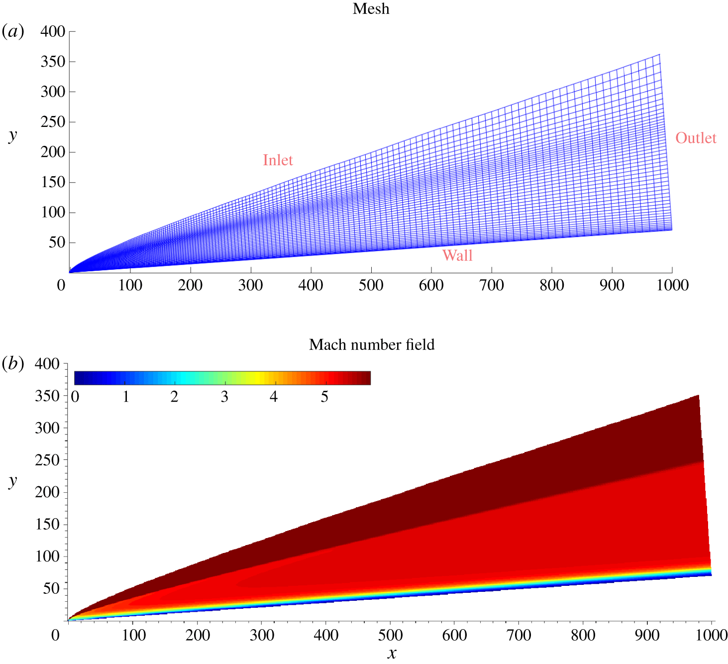
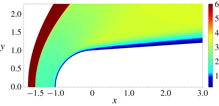
 $N_{x}\times N_{y}\times N_{z}=7920\times 150\times 100$. The distribution of the grid points in the wall-normal direction is controlled through a function that provides clustering in the shock region and towards the wall, in order to solve the captured shock wave and the boundary layer, as can be observed in figure 1(a). Figure 1(b) shows the computed Mach number field in a
 $xy$-plane. An iterative procedure is used to fit the shape of the computational domain with the computed shock, in order to reduce shock–grid misalignment. The grid points are also clustered in the
 $x$-direction to provide higher resolution near the leading edge, to resolve the strong bow shock and the local non-parallel effects in this region, and the streamwise variation of the wall-normal grid point distribution is controlled to better resolve the developing boundary layer. At
 $x=(200,400,600)$, the 99 % boundary-layer thickness is
 $\unicode[STIX]{x1D6FF}_{99}=(13.16,15.68,17.7)$ and the number of grid points within the boundary layer is
 $(45,37,33)$ resulting in a near-wall spacing to boundary-layer thickness ratio of
 $(0.0057,0.006,0.007)$. The grid design methodology is described in more detail in Cerminara (Reference Cerminara2017).
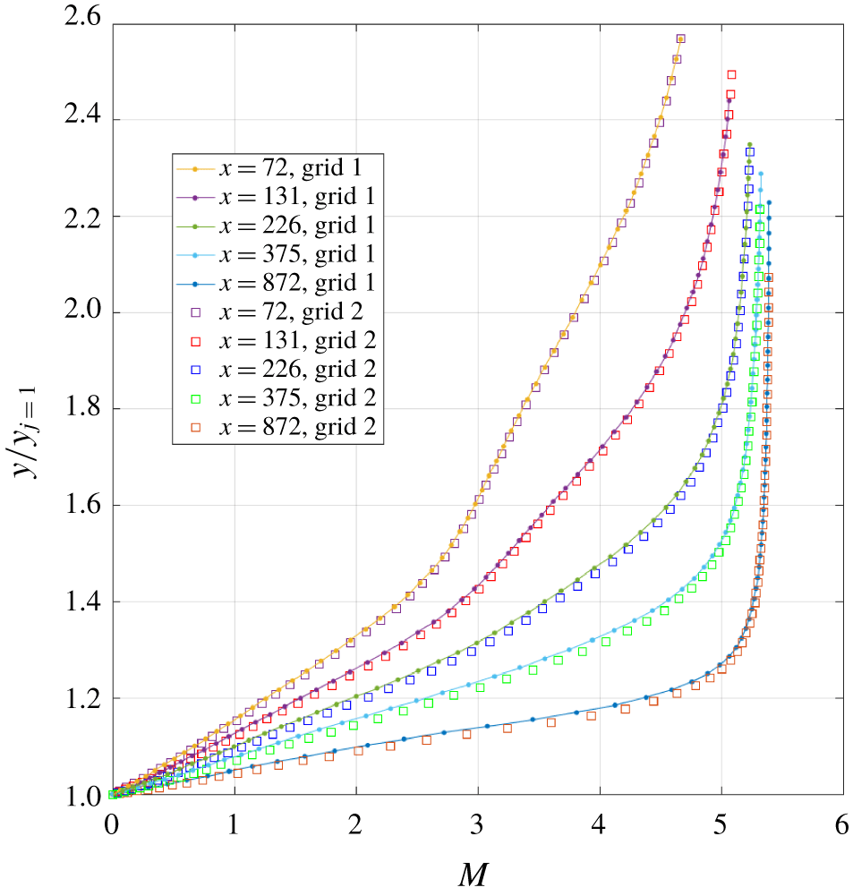
A grid study is shown in figure 2, based on the solution at different  $x$-positions of the boundary-layer Mach number profile for two different grids. Grid 1 refers to a coarser grid in the wall region, whereas grid 2 uses optimised grid stretching to provide higher resolution in the near-wall region. Figure 2 shows that a good agreement is reached at all the
 $x$-positions between the different grids.
View of the computational domain in a  $xy$-plane (a), and computed Mach number field (b). Note that the mesh has been plotted every 4 points in the
 $y$ direction and every 40 points in the
 $x$ direction.

Grid study between two grids without (grid 1) and with (grid 2) near-wall optimised grid stretching, for different  $x$ positions.

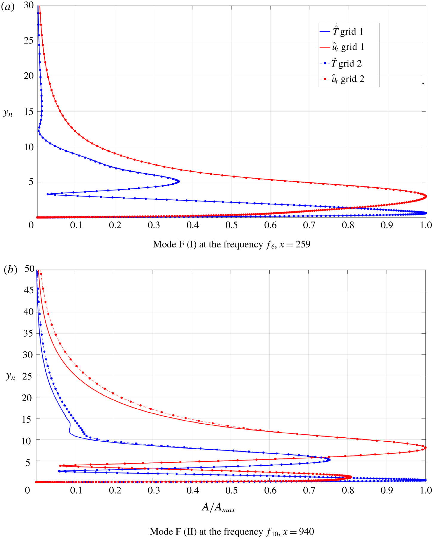
Grid sensitivity result for the temporal growth rate: mode F at  $x=259$ associated with frequency
 $f_{6}$,
 $\unicode[STIX]{x1D6FF}_{99}=13.46$.

Grid sensitivity in terms of the eigenfunctions of the linear stability analysis. Grid 1 and grid 2 are the coarser and the finer grids of the DNS base flow solution, respectively.

To better assess the suitability of the grid an additional grid sensitivity study was conducted based on results from linear stability analysis. In particular, we considered two reference streamwise positions, namely  $x=259$ and
 $x=940$. The former represents the peak location of mode F in frequency
 $f_{6}$ wall-pressure response (with reference to figure 6), whereas the latter is a downstream location where mode F II (i.e. the fast mode in its second excitation cycle) is dominant over the other internal modes in frequency
 $f_{10}$ response.
The boundary-layer profile of the base flow solution obtained from DNS at both the above mentioned locations for each grid is used as input profile for the local linear stability theory (LST) analyses. The result of the LST analyses will then provide the grid sensitivity of the eigenvalues and eigenfunctions. The local streamwise wavenumber of the fast acoustic waves outside of the boundary layer (i.e.  $\unicode[STIX]{x1D6FC}=2\unicode[STIX]{x03C0}f_{n}/(u_{t,e}+a_{e})$), at both the frequencies
 $f_{6}$ and
 $f_{10}$, has been used as input in the LST study at each position, with
 $u_{t,e}$ and
 $a_{e}$ being the local normalised wall-tangential velocity and speed of sound at the boundary-layer edge.
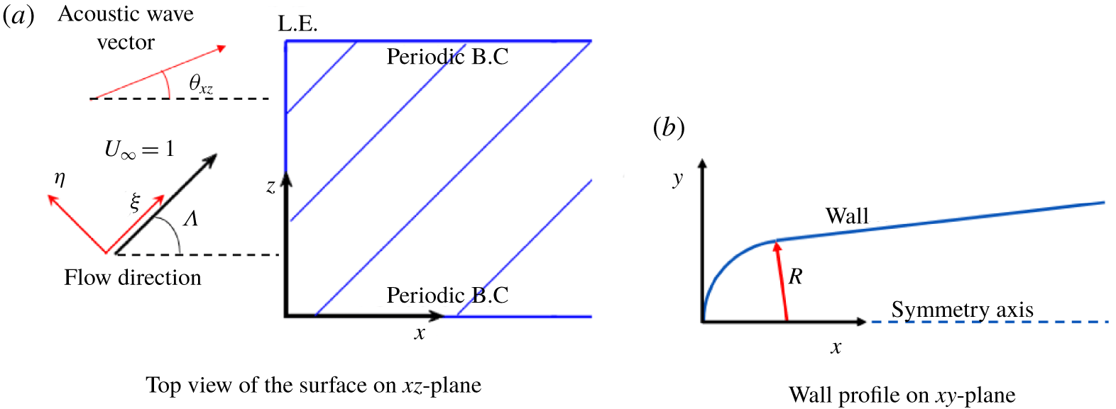
Sketch of a swept leading edge showing the orientation of the  $x$ axis in the chordwise direction and the
 $z$ axis in the spanwise direction, with the streamwise direction
 $\unicode[STIX]{x1D709}$ and the cross-flow direction
 $\unicode[STIX]{x1D702}$ shown for reference (a). Also shown is the surface profile in the
 $xy$-plane at the leading edge (b).

Grid sensitivity result for the temporal growth rate: mode F II at  $x=940$ associated with frequency
 $f_{10}$,
 $\unicode[STIX]{x1D6FF}_{99}=19.22$.

The results for the eigenvalue (i.e. the temporal growth rate,  $\unicode[STIX]{x1D714}_{i}$) and the eigenfunctions relative to the relevant fast modes at each location, namely mode F at
 $x=259$ and mode F II at
 $x=940$, have been obtained and compared between the different grids. The results of the grid sensitivity study are reported in tables 1 and 2 for the temporal growth rates, and in figure 3 for the eigenfunctions of the streamwise velocity and the temperature. Values of the ratio of the near-wall spacing to the boundary-layer thickness are also reported.
As can be seen, the near-wall resolution of grid 2 is approximately twice that of grid 1 at position  $x=259$, and is almost triple that of grid 1 at position
 $x=940$, thus highlighting the effects of the above mentioned optimised grid stretching in the near-wall region. We observe that the coarser grid provides a relative error in the temporal growth-rate solution, with respect to the reference finer grid (grid 2), of approximately 0.87 % at position
 $x=259$, and approximately 11.3 % at position
 $x=940$. The grid sensitivity study is further assessed in figure 3, in which the eigenfunctions for the wall-tangential velocity and temperature perturbations are plotted. For mode F at
 $x=259$ the eigenfunctions vary little between the grids. For mode F II at the position
 $x=940$, both the two near-wall peaks typical of mode F II are properly captured on the coarse grid, with the largest disagreements near the boundary-layer edge. Considering that position
 $x=940$ is close to the end of the computational domain, and that the frequency of mode F II (
 $f_{10}$) is the highest in the frequency spectrum, the errors at this location are representative of the worst case scenario. As such, considering that the receptivity process leading to breakdown occurs much further upstream, the errors can be considered acceptable for the purposes of the present study, in which all the simulations used the finer grid.
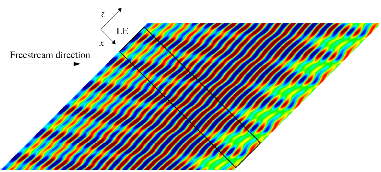
For the swept cases, with reference to the sketch in figure 4 and the illustration given in figure 5, a sweep angle of  $\unicode[STIX]{x1D6EC}=45^{\circ }$, between the streamwise direction
 $\unicode[STIX]{x1D709}$ of the flow and the chordwise direction, perpendicular to the leading edge, is considered. At the inflow, steady free-stream quantities are specified, superimposed where appropriate with time-dependent disturbances, as discussed in the next subsection. The reference velocity
 $U_{\infty }$ is aligned with the streamwise direction
 $\unicode[STIX]{x1D709}$. At the solid surface, a no-slip condition is applied to the velocity components, the temperature is set to the wall temperature (
 $T_{w}^{\ast }=300~\text{K}$). A symmetry condition is applied along the
 $y=0$ line upstream of the leading edge. At the outflow a zero gradient condition is applied along each grid line, while in the spanwise direction a periodic boundary condition is applied. The initial condition is taken as the free-stream condition and the simulations are run for long enough to allow any transient effect to wash through the domain.
2.5 Three-dimensional acoustic-wave model
The three-dimensional wave system consists of a main two-dimensional (2-D) wave and pairs of opposite-angle oblique waves of lower amplitude. The free-stream perturbation of the density as a function of time and Cartesian coordinates, for the case of multiple frequencies, is expressed as
 $$\begin{eqnarray}\unicode[STIX]{x1D70C}^{\prime }(x,z,t)=\mathop{\sum }_{m=0}^{M}\mathop{\sum }_{n=1}^{N}A_{m}\cos (\pm \unicode[STIX]{x1D6FD}_{m}z+\unicode[STIX]{x1D719}_{m,n})\cos (\unicode[STIX]{x1D6FC}_{n}x-\unicode[STIX]{x1D714}_{n}t+\unicode[STIX]{x1D713}_{n}),\quad (\unicode[STIX]{x1D6FD}_{0}=\unicode[STIX]{x1D719}_{0,n}=0),\end{eqnarray}$$
where  $\unicode[STIX]{x1D6FC}_{n}$ and
 $\unicode[STIX]{x1D6FD}_{m}$ are the wavenumbers, respectively, in the
 $x$ and
 $z$ directions,
 $\unicode[STIX]{x1D714}_{n}$ is the angular frequency,
 $A_{m}$ is the amplitude of each wave mode,
 $\unicode[STIX]{x1D719}_{m,n}$ and
 $\unicode[STIX]{x1D713}_{n}$ are randomly selected constant phase angles (an exception has to be made for
 $m=0$, for which
 $\unicode[STIX]{x1D719}_{m,n}$ is fixed to zero),
 $N$ and
 $M$ represent the total number of frequencies and (non-zero) spanwise wavenumbers respectively, while the subscripts ‘
 $m$’ and ‘
 $n$’ indicate the
 $m$th spanwise wave mode and the
 $n$th frequency respectively. In the present study
 $N=10$, indicating a spectrum of 10 different frequencies, and
 $M=2$, with spanwise wavenumbers given by
 $\unicode[STIX]{x1D6FD}_{m}=2\unicode[STIX]{x03C0}m/L_{z}$ (with
 $L_{z}=55$ being the length of the domain in the
 $z$ direction);
 $N$ and
 $M$ were chosen to capture the relevant unstable modes, relative to the range of frequencies and wave angles, for the considered flow. Note that
 $m=0$ provides a two-dimensional wave in the body reference system, as
 $\unicode[STIX]{x1D6FD}_{0}=0$ and
 $\unicode[STIX]{x1D719}_{0,n}=0$, namely a wave whose wave vector is aligned with the
 $x$-axis of the body reference system. However, as
 $x$ is perpendicular to the leading edge, for swept cases such a wave mode (
 $m=0$) represents an oblique wave with respect to the streamwise direction, with an inclination angle equal to the sweep angle (
 $\unicode[STIX]{x1D6EC}$) of the leading edge. An illustrative example of an infinite swept leading edge and of the domain geometry is shown in figure 5. Here, the black lines represent the edges of the computational domain on a
 $xz$-plane. Note that the
 $x$-axis is perpendicular to the leading edge.
Illustrative example of an infinite swept leading edge ( $\unicode[STIX]{x1D6EC}=45^{\circ }$). The black lines indicate the edges of the computational domain on the body surface in the
 $xz$-plane. The contours are relative to a solution for the wall-pressure fluctuations.

The wavenumber in the  $x$-direction
 $\unicode[STIX]{x1D6FC}_{n}$ is linked to the angular frequency
 $\unicode[STIX]{x1D714}_{n}$ through the relation
 $\unicode[STIX]{x1D6FC}_{n}=\unicode[STIX]{x1D714}_{n}/(\cos \unicode[STIX]{x1D6EC}\pm 1/M)$, with
 $\unicode[STIX]{x1D714}_{n}=2\unicode[STIX]{x03C0}f_{n}$, being
 $f_{n}$ the
 $n$th frequency of the forcing spectrum. The term
 $\cos \unicode[STIX]{x1D6EC}\pm 1/M$ represents the dimensionless phase speed along the
 $x$-axis of the free-stream waves, where the plus sign indicates fast acoustic waves and the minus sign stands for slow acoustic waves. Hence, an oblique acoustic wave travelling with an inclination angle
 $\unicode[STIX]{x1D703}_{xz}$ with respect to the
 $x$-axis has a wavenumber
 $\unicode[STIX]{x1D6FC}$ in the
 $x$ direction, equal to the corresponding wavenumber of the dominant 2-D fast or slow acoustic wave. The value of
 $A_{0}$ determines the amplitude of the main 2-D wave, while the amplitude of each pair of oblique waves for
 $m=1,2$ is linked to that of the 2-D wave through the relation
 $A_{1}=A_{2}={\textstyle \frac{1}{2}}A_{0}$. For each non-zero spanwise wavenumber two oblique acoustic waves with equal and opposite angles
 $\unicode[STIX]{x1D703}_{xz}$ are forced, and the amplitude
 $A_{m}$ (for
 $m=1,2$) represents the sum of the amplitudes of the two opposite-angle waves, such that each single oblique wave has an amplitude equal to
 ${\textstyle \frac{1}{4}}A_{0}$.
The value of the inclination angle of the forced oblique waves in the  $xz$-plane for each spanwise wavenumber (
 $m$) and for each frequency (
 $n$) is given by
 $$\begin{eqnarray}\unicode[STIX]{x1D703}_{xz}^{m,n}=\pm \arctan \left(\frac{\unicode[STIX]{x1D6FD}_{m}}{\unicode[STIX]{x1D6FC}_{n}}\right).\end{eqnarray}$$
For the fast acoustic waves, the wave angle for the complete spectrum of oblique waves spans a range from approximately  $23^{\circ }$ to
 $67^{\circ }$, according to (2.15), whereas for slow acoustic waves the range is from approximately
 $16^{\circ }$ to
 $60^{\circ }$. The most unstable oblique modes (e.g. the oblique first modes) are included in these ranges, hence they can be captured by the prescribed spectrum of streamwise and spanwise wavenumbers. Waves with a higher wave angle (i.e. outside the considered ranges) are not expected to make a significant contribution to the transition process.
Finally, the vector of the conservative variables at the inflow boundary in the unsteady 3-D computations is given by
 $$\begin{eqnarray}\boldsymbol{Q}^{U}=\left[\begin{array}{@{}c@{}}\unicode[STIX]{x1D70C}_{\infty }+\unicode[STIX]{x1D70C}_{\infty }^{\prime }\\ (\unicode[STIX]{x1D70C}_{\infty }+\unicode[STIX]{x1D70C}_{\infty }^{\prime })(u_{\infty }+u_{\infty }^{\prime })\\ (\unicode[STIX]{x1D70C}_{\infty }+\unicode[STIX]{x1D70C}_{\infty }^{\prime })(v_{\infty }+v_{\infty }^{\prime })\\ (\unicode[STIX]{x1D70C}_{\infty }+\unicode[STIX]{x1D70C}_{\infty }^{\prime })(w_{\infty }+w_{\infty }^{\prime })\\ (\unicode[STIX]{x1D70C}_{\infty }+\unicode[STIX]{x1D70C}_{\infty }^{\prime })(E_{\infty }+E_{\infty }^{\prime })\end{array}\right].\end{eqnarray}$$
Since the two opposite-angle waves travel in opposite directions along the  $z$-axis, their free-stream
 $z$-velocity perturbation cancels, so that
 $w_{\infty }^{\prime }=0$ identically. Also, the free-stream perturbation of the
 $y$-velocity component
 $v_{\infty }^{\prime }$ is fixed to zero, as all the waves are taken to travel in the direction parallel to the
 $xz$-plane. The dispersion relations that link the velocity components, pressure and total energy fluctuations to the density fluctuation are derived from the linearised Euler equations with the assumption of small perturbations (Cerminara & Sandham Reference Cerminara and Sandham2015, Reference Cerminara and Sandham2017). These relations are as follows,
 $$\begin{eqnarray}u_{\infty }^{\prime }=\frac{1}{M}\unicode[STIX]{x1D70C}_{\infty }^{\prime }\cos \unicode[STIX]{x1D703}_{xz},\quad v_{\infty }^{\prime }=0,\quad w_{\infty }^{\prime }=0,\end{eqnarray}$$
 $$\begin{eqnarray}p_{\infty }^{\prime }=\frac{1}{M^{2}}\unicode[STIX]{x1D70C}_{\infty }^{\prime },\quad E_{\infty }^{\prime }=\frac{1}{M}\unicode[STIX]{x1D70C}_{\infty }^{\prime }\left(\frac{1}{\unicode[STIX]{x1D6FE}M}+\cos \unicode[STIX]{x1D6EC}\cos \unicode[STIX]{x1D703}_{xz}\right).\end{eqnarray}$$
These relations are consistent with those given in Egorov, Sudakov & Fedorov (Reference Egorov, Sudakov and Fedorov2006), as the same normalisation for the pressure is used, i.e.  $p_{\infty }=p_{\infty }^{\ast }/(\unicode[STIX]{x1D70C}_{\infty }^{\ast }U_{\infty }^{\ast 2})$. Note that in other works, e.g. in Zhong & Ma (Reference Zhong and Ma2006), the normalisation of the pressure with the free-stream pressure leads to a different relation with the density fluctuation (i.e.
 $p_{\infty }^{\prime }=\unicode[STIX]{x1D6FE}\unicode[STIX]{x1D70C}_{\infty }^{\prime }$).
2.6 Simulated cases
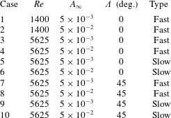
A total of ten numerical simulations have been carried out, as detailed in table 3. The lower Reynolds number cases (at  $Re=1400$ based on the nose radius) are used to confirm the leading-edge receptivity to fast acoustic waves and check the influence of the disturbance amplitude
 $A_{\infty }$. The higher Reynolds number,
 $Re=5625$, is within the range of the Reynolds numbers considered in the transition experiments of Durant et al. (Reference Durant, André, Schneider and Chynoweth2015). The receptivity to both fast and slow acoustic waves is studied, and for each case both higher-amplitude and smaller-amplitude free-stream disturbances have been applied, so that four cases have been run overall at this Reynolds number in an unswept
 $\unicode[STIX]{x1D6EC}=0^{\circ }$ configuration. A further four cases, comprising fast and slow free-stream acoustic waves at two different amplitudes, have been run at the same Reynolds number for the swept configuration. For each case the Mach number is
 $M=6$, the free-stream temperature is set to
 $T_{\infty }^{\ast }=51.7~\text{K}$. These conditions are intended to simulate the free-stream conditions of a typical low enthalpy hypersonic wind tunnel.
Settings of the numerical simulations.

Different frequencies are inserted in the free-stream forcing, according to (2.14), with each frequency being an integer multiple of  $f_{0}=3.509\times 10^{-3}$. The frequency
 $f$ is already in the form of a dimensionless Strouhal number,
 $f=f^{\ast }R^{\ast }/U_{\infty }^{\ast }$. The spectrum of the forced frequencies spans from
 $f_{1}=5f_{0}$ to
 $f_{10}=14f_{0}$. The non-dimensional frequency in its standard definition,
 $F_{s}=2\unicode[STIX]{x03C0}f^{\ast }\unicode[STIX]{x1D707}_{\infty }^{\ast }/(\unicode[STIX]{x1D70C}_{\infty }^{\ast }U_{\infty }^{\ast 2})$, can be obtained from
 $F_{s}=2\unicode[STIX]{x03C0}f/Re$. The chosen frequency spectrum is partly based on linear stability studies conducted by De Tullio & Sandham (Reference De Tullio and Sandham2015) for a flow at Mach 6 over a flat plate with a Reynolds number comparable with our
 $Re=1400$ case. In particular, at this Reynolds number, the frequencies from
 $f_{5}$ to
 $f_{10}$ covers the range of the most unstable second mode frequencies. At the higher Reynolds number case, for a nose radius representative of the experimental probe tested in Durant et al. (Reference Durant, André, Schneider and Chynoweth2015), i.e.
 $R^{\ast }=1.2~\text{mm}$, this frequency range covers the frequency range typical of the unstable travelling cross-flow waves (
 $f^{\ast }<35~\text{kHz}$), which is relevant for the swept wedge case. The amplitudes of
 $v_{\infty }^{\prime }$ and
 $w_{\infty }^{\prime }$ are identically zero in the free stream, as the imposed acoustic waves propagate in the
 $xz$-plane with a 2-D component (namely a wave oriented along the
 $x$-axis) and two pairs of oblique waves with the same amplitude and opposite angles (namely
 $\unicode[STIX]{x1D703}_{xz}$ and
 $-\unicode[STIX]{x1D703}_{xz}$). The present configuration of the free-stream disturbance allows the use of multiple streamwise and spanwise wavenumbers of the acoustic waves, which can be kept fixed while the sweep angle is changed, so that changes in the response can be ascribed to the effect of sweep. In a wider parametric study one would also want to vary the incidence and side angles and choose a wider selection of spanwise wavenumbers.
For each frequency, the free-stream amplitude of the 2-D wave (based on the density) is set to  $A_{0}=2.5\times 10^{-2}$ in the high-amplitude case, and to
 $A_{0}=2.5\times 10^{-3}$ in the low-amplitude case. As described in § 2.5, each oblique wave is set with an amplitude of
 $1/4$ that of the main 2-D wave, resulting in an amplitude of
 $1/2$ for each pair of opposite-angle oblique waves, namely
 $A_{1}=A_{2}=1.25\times 10^{-2}$ and
 $A_{1}=A_{2}=1.25\times 10^{-3}$ for high and low amplitudes respectively. Hence, the overall maximum amplitude of the wave system (i.e.
 $A_{\infty }=A_{0}+A_{1}+A_{2}$) is
 $A_{\infty }=5\times 10^{-2}$ and
 $A_{\infty }=5\times 10^{-3}$ for high and low amplitudes respectively. The corresponding root-mean-square of the high-amplitude signal composed of the 2-D and oblique wave modes are 2 % and 2.8 % for the density and pressure fluctuations respectively.
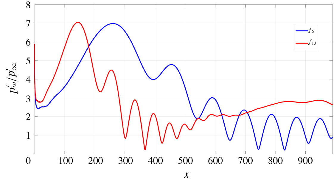
Wall-pressure fluctuation amplitude for fast acoustic waves, at the frequencies  $f_{6}$ and
 $f_{10}$.
 $A_{\infty }=5\times 10^{-3}$, Case 1, 2-D wave (
 $\unicode[STIX]{x1D6FD}=0$).

While it is not possible to match inflow disturbances of this form to any experiment, it can be noted that the overall magnitude (5 %) of the inflow wave system for the high amplitude is of the same order as that measured by Masutti et al. (Reference Masutti, Spinosa, Chazot and Carbonaro2012) (4.9 %) for the density fluctuations in the Mach 6 blowdown facility at the von Karman Institute (VKI). Within this overall level, the 3-D modes have an amplitude (0.625 %) similar to the levels reported by Parziale et al. (Reference Parziale, Shepherd and Hornung2014), who measured density levels of 0.5 % for the Mach 5.5 flow in a T5 reflected-shock tunnel, Duan et al. (Reference Duan, Choudhari and Wu2014), who computed a value of 0.39 % for the pressure fluctuations radiated by a turbulent boundary layer in a Mach 2.5 flow, and Wagner et al. (Reference Wagner, Schülein, Petervari, Hannemann, Ali, Cerminara and Sandham2018), who estimated a similar value of 0.48 % for the noise in a Mach 3 flow in the case of dominant slow acoustic waves, using a combined experimental–numerical approach.
3 Results for the unswept wedge
In this section we focus on the receptivity and breakdown mechanisms in the unswept configuration using DNS and LST. Figure 6 shows an example of the wall-pressure variations obtained from DNS for case 1 listed in table 1. The time-dependent pressure has been Fourier transformed in time and the amplitudes are shown for two of the frequencies that were forced at the inflow. In both cases we see an initial growth as disturbances penetrate into the boundary layer, followed by oscillatory behaviour, which has previously (Cerminara & Sandham Reference Cerminara and Sandham2017) been attributed to a modulation process based on the presence of multiple boundary-layer modes, consistent with the findings of Ma & Zhong (Reference Ma and Zhong2005) and Zhong & Ma (Reference Zhong and Ma2006). Our initial objective is to place the observed receptivity process in the context of the mechanisms identified in the theoretical work of Fedorov & Khokhlov (Reference Fedorov and Khokhlov2001), Fedorov (Reference Fedorov2003) and Fedorov (Reference Fedorov2011), and the simulation work of Zhong (Reference Zhong2001), Ma & Zhong (Reference Ma and Zhong2003a), Ma & Zhong (Reference Ma and Zhong2003b), Ma & Zhong (Reference Ma and Zhong2005), Zhong & Ma (Reference Zhong and Ma2006), and Zhong & Wang (Reference Zhong and Wang2012). We will then consider the nonlinear stages of the breakdown process at higher Reynolds numbers for both fast and slow acoustic disturbances.
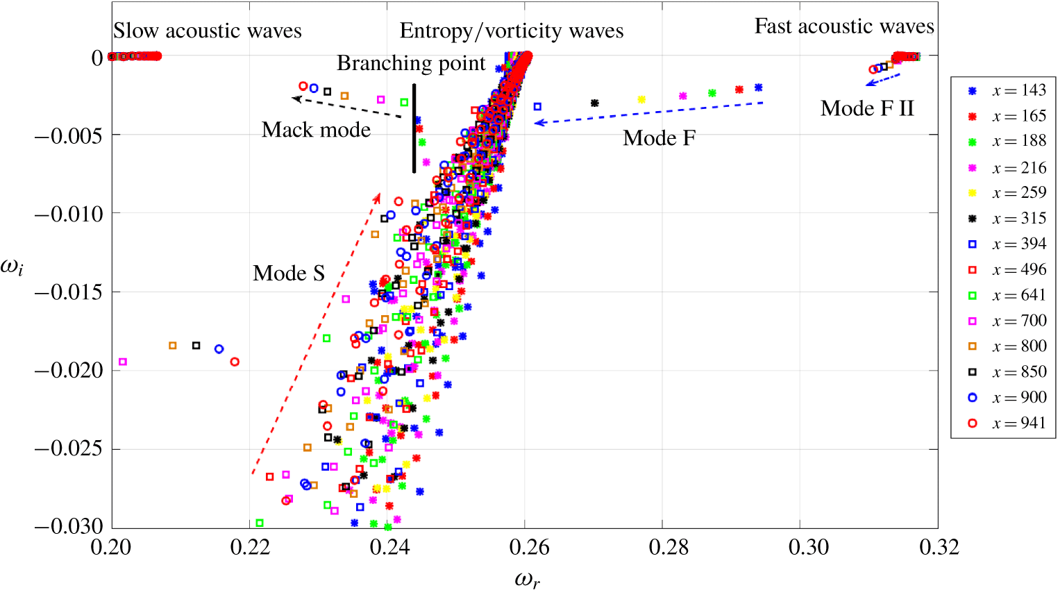
Spectrum of the eigenvalues at the frequency  $f_{10}$, 2-D wave (
 $\unicode[STIX]{x1D6FD}=0$).

3.1 Formation of boundary-layer modes
Local stability analysis, based on the temporal approach, has been carried out at different streamwise locations, corresponding to the frequencies  $f_{6}$ and
 $f_{10}$ shown in figure 6, for two-dimensional disturbances (i.e.
 $\unicode[STIX]{x1D6FD}=0$). The streamwise wavenumbers for the LST analysis were computed from
 $\unicode[STIX]{x1D6FC}_{n}=2\unicode[STIX]{x03C0}f_{n}/(u_{t,e}+a_{e})$, where
 $u_{t,e}$ and
 $a_{e}$ are respectively the local wall-tangential velocity component and speed of sound at the boundary-layer edge at each considered
 $x$-location. The considered phase speed for the LST analysis corresponds to the local fast-mode phase speed, thus resulting in the local streamwise wavenumber of the fast acoustic waves outside the boundary layer (i.e. the local forcing) being used as input for the LST analysis at all the streamwise locations at both the frequencies
 $f_{6}$ and
 $f_{10}$. Figure 7 shows the spectrum of the complex eigenvalues at different positions along the wedge for the frequency
 $f_{10}$. Moving from low to high values of
 $\unicode[STIX]{x1D714}_{r}$ in the spectrum corresponds to moving from low to high phase speeds(i.e. the output phase speeds of the LST analysis). The two horizontal branches of modes at
 $\unicode[STIX]{x1D714}_{i}\approx 0$ positioned at the left and right extremes of the graph represent the slow and fast acoustic-wave continuous spectra respectively. The branch of modes positioned in the middle of the graph, at approximately
 $\unicode[STIX]{x1D714}_{r}=0.26$, represents the entropy/vorticity wave continuous spectrum.
Performing the LST analysis at several  $x$ positions is equivalent to tracking the movement of some discrete modes of interest. The evolution of the discrete modes helps, in turn, to understand the corresponding trend of the numerical pressure distribution shown in figure 6. In particular, at the streamwise location corresponding to the first peak (
 $x\approx 150$) in the curve of the pressure response, figure 7 shows the presence of a discrete stable mode close to the continuous spectrum of the fast acoustic waves (the blue asterisk symbol, indicating the position
 $x=143$, with
 $\unicode[STIX]{x1D714}_{r}=0.294$). This mode corresponds to mode F, which is synchronised with the forced fast acoustic waves in the leading-edge region, thus experiencing a resonance-induced amplification (Fedorov & Khokhlov Reference Fedorov and Khokhlov2001), as shown by the numerical results. However, as is evident in figure 7, mode F gradually moves away from the fast acoustic-wave continuous spectrum, corresponding to a de-synchronisation process. This results in a downstream decay of the wall response, due to the decay of mode F, which decreases its phase speed (as it moves towards lower values of
 $\unicode[STIX]{x1D714}_{r}$) and becomes more stable (moving towards higher negative values of
 $\unicode[STIX]{x1D714}_{i}$).
The region  $x\approx 250{-}500$ is characterised by an oscillatory wall response in figure 6 (for frequency
 $f_{10}$) that suggests a modulation process as mode F traverses the entropy/vorticity wave continuous spectrum. Such a behaviour was previously observed in Ma & Zhong (Reference Ma and Zhong2003b), Ma & Zhong (Reference Ma and Zhong2005), Zhong & Ma (Reference Zhong and Ma2006) and Zhong & Wang (Reference Zhong and Wang2012), and described as a modulation between different competing modes, such as the internal decayed mode F and the external mode of the forcing fast acoustic waves. At the same time, another discrete mode, close to the slow acoustic-wave continuous spectrum, starts moving rapidly from very low values of
 $\unicode[STIX]{x1D714}_{i}$ to higher values, becoming less stable with increasing phase speed. This mode corresponds to mode S, which is excited due to a synchronisation with the decaying mode F, after the latter has crossed the convected wave continuous spectrum.
Upstream of  $x=641$ mode S corresponds still to the first (lower-frequency) instability mode, then for
 $x>641$ mode S develops in a second (higher-frequency) instability mode (or Mack mode) (Mack Reference Mack1984), which emerges as a consequence of the wavelength exchange (or synchronisation) mechanism between mode F and mode S (Fedorov & Khokhlov Reference Fedorov and Khokhlov2001; Fedorov Reference Fedorov2003, Reference Fedorov2011; Ma & Zhong Reference Ma and Zhong2003a,Reference Ma and Zhongb, Reference Ma and Zhong2005; Zhong & Ma Reference Zhong and Ma2006; Fedorov & Tumin Reference Fedorov and Tumin2011; Zhong & Wang Reference Zhong and Wang2012). Further downstream, the Mack mode shows a decreasing frequency (and phase speed), and becomes progressively less stable. Downstream of
 $x=700$ in figure 6, the
 $f_{10}$ curve appears now much smoother than in the previous modulation region, which indicates that there is a dominant mode in this region. This mode grows as a consequence of a resonance, due to a (second) synchronisation with the fast acoustic waves, consistent with the numerical results of Ma & Zhong (Reference Ma and Zhong2003b), Ma & Zhong (Reference Ma and Zhong2005), Zhong & Ma (Reference Zhong and Ma2006) and Zhong & Wang (Reference Zhong and Wang2012). For this reason, we refer to this mode as the second fast mode, or mode F II, combining both Fedorov’s and Zhong’s notation (Fedorov Reference Fedorov2011; Zhong & Wang Reference Zhong and Wang2012). The downstream evolution of the second fast mode is represented by a short branch very close to the fast acoustic-wave continuous spectrum in the top right corner of figure 7.
Similar characteristics have been observed in the corresponding spectrum at the frequency  $f_{6}$, with the difference that the evolution of the modes is delayed and extends only up to approximately the position where mode F traverses the convected wave continuous spectrum, as can be observed in figure 6. Thus, the evolution of the boundary-layer modes at the higher frequencies is quicker than at the lower frequencies, and results in the mode F/mode S wavelength exchange mechanism taking place closer to the leading edge.
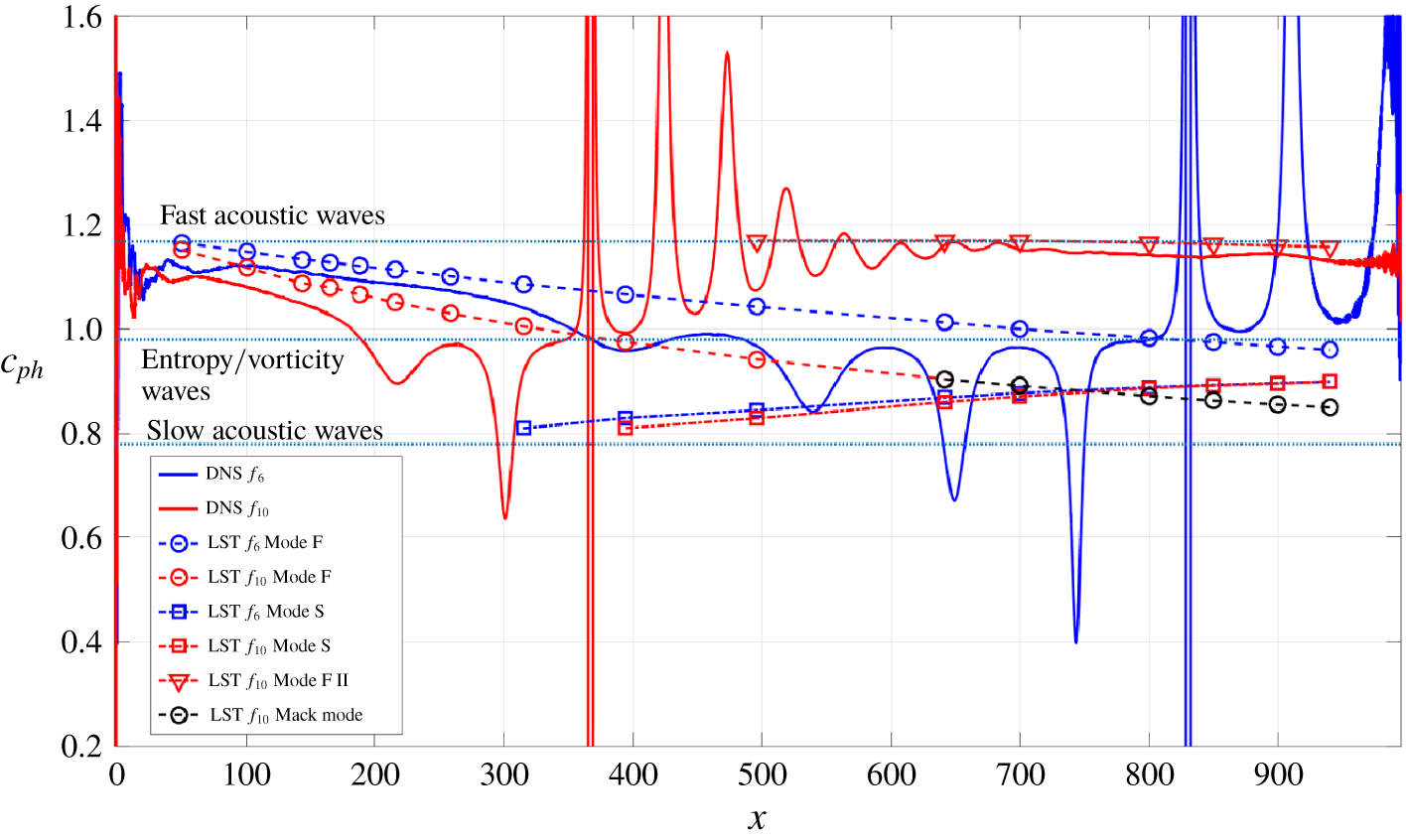
Phase speed of the boundary-layer modes along the wall for the frequencies  $f_{6}$ and
 $f_{10}$. Comparison between DNS and LST results. The dotted horizontal blue lines indicate the local phase-speed values of the fast and slow acoustic waves, and the entropy/vorticity waves.

An alternative perspective on these processes is provided by figure 8, which shows a comparison between the DNS and the LST phase speeds at both the frequencies  $f_{6}$ and
 $f_{10}$. Similar plots have been presented by Ma & Zhong (Reference Ma and Zhong2003b), Ma & Zhong (Reference Ma and Zhong2005), Zhong & Ma (Reference Zhong and Ma2006) and Zhong & Wang (Reference Zhong and Wang2012). The phase speed from the DNS results has been computed through the fast Fourier transformed wall-pressure fluctuations, using the relation for the streamwise wavenumber
 $$\begin{eqnarray}\unicode[STIX]{x1D6FC}(x,f)=\unicode[STIX]{x1D6FC}_{r}+\text{i}\unicode[STIX]{x1D6FC}_{i}=\frac{1}{\text{i}p_{w}^{\prime }(x,f)}\frac{\unicode[STIX]{x2202}p_{w}^{\prime }(x,f)}{\unicode[STIX]{x2202}x},\end{eqnarray}$$
and then applying the relation  $c_{ph}=2\unicode[STIX]{x03C0}f/\unicode[STIX]{x1D6FC}_{r}$. For both the frequencies, the numerical phase speed (represented by blue and red solid lines for the frequencies
 $f_{6}$ and
 $f_{10}$ respectively) starts at a value of approximately 1.12 in the early nose region. This is slightly lower than the local fast acoustic-wave phase speed of approximately 1.16, which is attributed to non-parallel effects in the early leading-edge region. For
 $x>100$ both LST and DNS follow the same decreasing trend and it can be concluded that the internal mode generated at the leading edge is mode F.
Further downstream (for  $x>200$ at
 $f_{10}$ and
 $x>400$ at
 $f_{6}$) an oscillatory behaviour is seen in figure 8 that can be explained by mode F traversing the convected wave continuous spectrum and entering a synchronisation process with the internal mode S. Here, the numerical phase speed shows a rapid increase, and a second synchronisation with the local fast acoustic waves is reached. Downstream of this synchronisation point (
 $x=370$ at the frequency
 $f_{10}$, and
 $x=830$ at the frequency
 $f_{6}$), the numerical phase speed no longer follows the LST result for mode F, but instead agrees very well with the LST result for mode F II, as can be seen further downstream for the frequency
 $f_{10}$ (for the lower frequency,
 $f_{6}$, mode F II would be reached further downstream of the computational domain outer edge). During the decay of mode F, when the phase speed drops below the value of 0.9, strong oscillations of the numerical solution are observed, as a consequence of the mode F phase speed approaching the phase speed of mode S, which results in an initial growth of the latter, as shown by the LST curves representing mode S (blue and red dash-dot curves with square symbols). These oscillations represent the modulation process between the forcing fast acoustic waves and the decaying mode F, in the region where the latter is synchronised with mode S. Downstream of the intersection point between mode F and mode S LST phase speeds (i.e. the mode F–mode S synchronisation point) at the frequency
 $f_{10}$, the Mack mode is generated and develops downstream with an initial decrease of the phase speed, as a continuation of the mode F branch, but with increasing growth rate. These results are qualitatively in a very good agreement with the results of Ma & Zhong (Reference Ma and Zhong2005), Zhong & Ma (Reference Zhong and Ma2006) and Zhong & Wang (Reference Zhong and Wang2012).
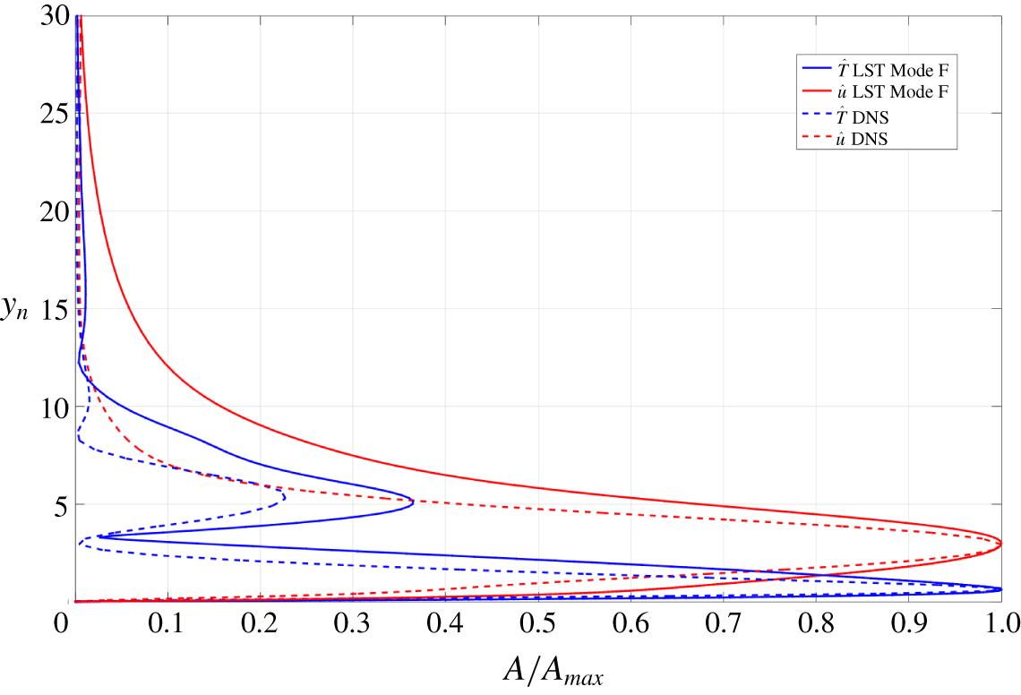
A further comparison between the DNS and the LST results, including a more detailed identification of the internal modes, is made by considering the eigenfunctions of the different modes. Figure 9 shows the temperature  $\hat{T}$ and wall-tangential velocity
 $\hat{u}$ eigenfunctions (normalised with the maximum inside the boundary layer as
 $A/A_{max}$) for the frequency
 $f_{6}$ at
 $x=259$, which is the position from figure 6 where the first peak of the wall-pressure fluctuation amplitude is reached due to the resonance between leading-edge fast-acoustic mode and mode F. At this position mode F is the dominant mode inside the boundary layer, which is proved by the good agreement between the DNS results for
 $\hat{T}$ and
 $\hat{u}$ and the LST eigenfunctions for mode F. As can be seen, the shape of mode F is characterised by a high peak near the wall. These results are also in a good qualitative agreement with the numerical and LST results of Zhong (Reference Zhong2001) for the eigenfunctions of mode F. In the modulation regions the comparison between the DNS profiles and the eigenfunctions from the LST is not as good since no dominant mode exists. In conclusion, the present numerical and theoretical results show the main characteristics of Fedorov’s (Fedorov & Khokhlov Reference Fedorov and Khokhlov2001; Fedorov Reference Fedorov2003) receptivity mechanism for hypersonic boundary layers, and are in good qualitative agreement with other theoretical and numerical studies available in the literature (Zhong Reference Zhong2001; Ma & Zhong Reference Ma and Zhong2005; Zhong & Ma Reference Zhong and Ma2006; Fedorov Reference Fedorov2011; Zhong & Wang Reference Zhong and Wang2012), for different flow conditions.
Temperature and wall-tangential velocity eigenfunctions for the frequencies  $f_{6}$ at the position
 $x=259$.

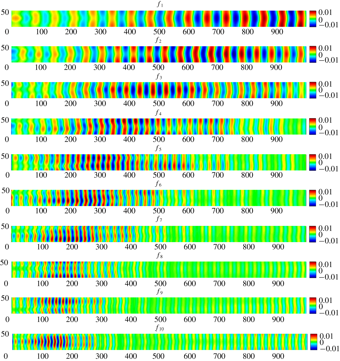
Real part of the Fourier-transformed wall-pressure fluctuations ( $p_{w}^{\prime }$) at the different forced frequencies. Case 1,
 $A_{\infty }=5\times 10^{-3}$. The labels of the vertical (
 $z$) and horizontal (
 $x$) axes have been purposely omitted.

3.2 Disturbance growth and breakdown mechanism
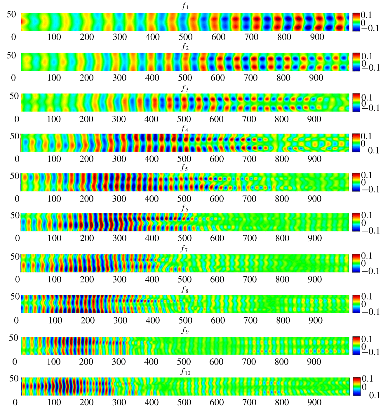
The DNS allows the transition process to be followed up to final breakdown to turbulence. We start by illustrating the results of the 3-D simulations for the cases at lower Reynolds number with fast acoustic waves as free-stream disturbances (cases 1 and 2 from table 3). Figures 10 and 11 show contours of the real part of the Fourier-transformed wall-pressure fluctuations at all the considered frequencies (from  $f_{1}$ at the top to
 $f_{10}$ at the bottom) for cases at lower (case 1) and higher (case 2) free-stream disturbance amplitude respectively. Moving from top to bottom in both figures, the effect of frequency on the resonance mechanism can be seen, with the peak wall disturbance amplitude moving towards the leading edge as the frequency is increased. In the lower-amplitude case (figure 10) the wall disturbances appear to be dominated by a 2-D mode through the whole length of the computational domain. In contrast, in the higher-amplitude case (figure 11) the 2-D mode seems to be the most amplified mode only in the leading-edge region and, once the peak has been achieved, 3-D modes (with non-zero spanwise wavenumber) emerge and become the dominant structures further downstream. The solution in the nose region (
 $x=0{-}200$) is similar between the two different amplitude cases at all the frequencies, with the contour levels scaled by the same one order of magnitude as for the forcing. This means that the solution can be reasonably considered as linear in the early region of the computational domain. Further downstream, the solution becomes different between the cases at different amplitude, meaning that nonlinear effects are no longer negligible. The nonlinearity appears first in the form of long streaky structures that reduce the spanwise coherence of the waves and are seen for all the considered frequencies.
Real part of the Fourier-transformed wall-pressure fluctuations ( $p_{w}^{\prime }$) at the different forced frequencies. Case 2,
 $A_{\infty }=5\times 10^{-2}$. The labels of the vertical (
 $z$) and horizontal (
 $x$) axes have been purposely omitted.

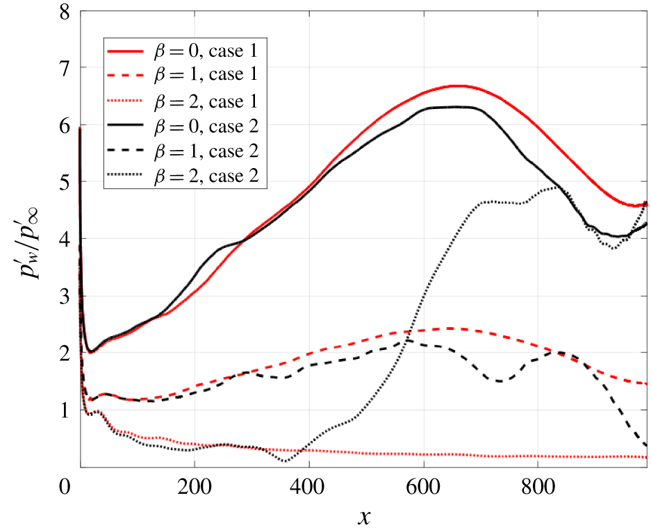
Figure 12 shows the trend of the wall-pressure fluctuation amplitudes along the wedge for the modes  $\unicode[STIX]{x1D6FD}=0,1,2$ at the frequency
 $f_{2}$ for both high- and low-amplitude cases, obtained through a fast Fourier transform (FFT) in time and in the spanwise direction. The wall-pressure fluctuation amplitudes for each mode are normalised with the value of the corresponding free-stream pressure fluctuation amplitude (i.e. as
 $p_{w}^{\prime }/p_{\infty }^{\prime }$). The wall response very close to the leading edge does not show a significant difference between case 1 and case 2, due to the nonlinear effects being relatively small in this region. In the second half of the computational domain, in contrast, the large nonlinear effects in case 2 provide a markedly different behaviour. In particular, the
 $\unicode[STIX]{x1D6FD}=2$ mode decays to very low values in case 1, whilst in case 2 it is strongly excited in the second half of the domain. Also, it is evident that the rapid growth of the
 $\unicode[STIX]{x1D6FD}=2$ mode starts at a position very close to the point where the peak of the 2-D mode F is reached, thus suggesting that the resonance mechanism at the leading edge might play an important role in the excitation of 3-D boundary-layer disturbances. In fact, it is evident in figure 12 and also from comparison between figures 10 and 11 that as soon as the disturbance amplitude reaches its maximum value (corresponding to the peak of mode F resulting from the resonance mechanism) 3-D disturbances are generated and the response pattern in the high-amplitude case diverges from that in the low-amplitude case. This suggests that in the high-amplitude case, the resonance mechanism increases the amplitude to values high enough to trigger nonlinear effects that affects the wall response (and the associated breakdown mechanism) further downstream. The associated flow structure is revealed by figure 13, which shows an instantaneous contour of the wall-tangential velocity component (
 $u_{t}$) for the
 $j=10$ grid line inside the boundary layer. It is evident that the excitation of the
 $\unicode[STIX]{x1D6FD}=2$ mode at the different forcing frequencies corresponds to the generation and downstream growth of streaks in the streamwise direction inside the boundary layer. For the low Reynolds number cases considered so far, these streaks do not break down within the computational domain, so we turn next to the higher Reynolds number cases 3–6 from table 1.
Extracted modes ( $\unicode[STIX]{x1D6FD}=0,1,2$) of the wall-pressure fluctuation amplitudes at the frequency
 $f_{2}$, for cases 1 and 2.

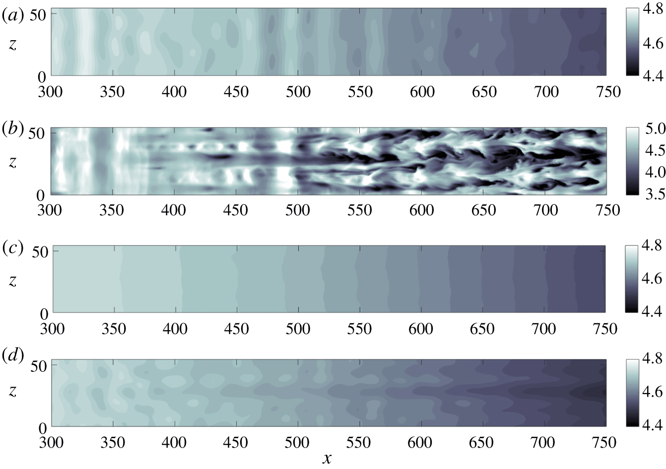
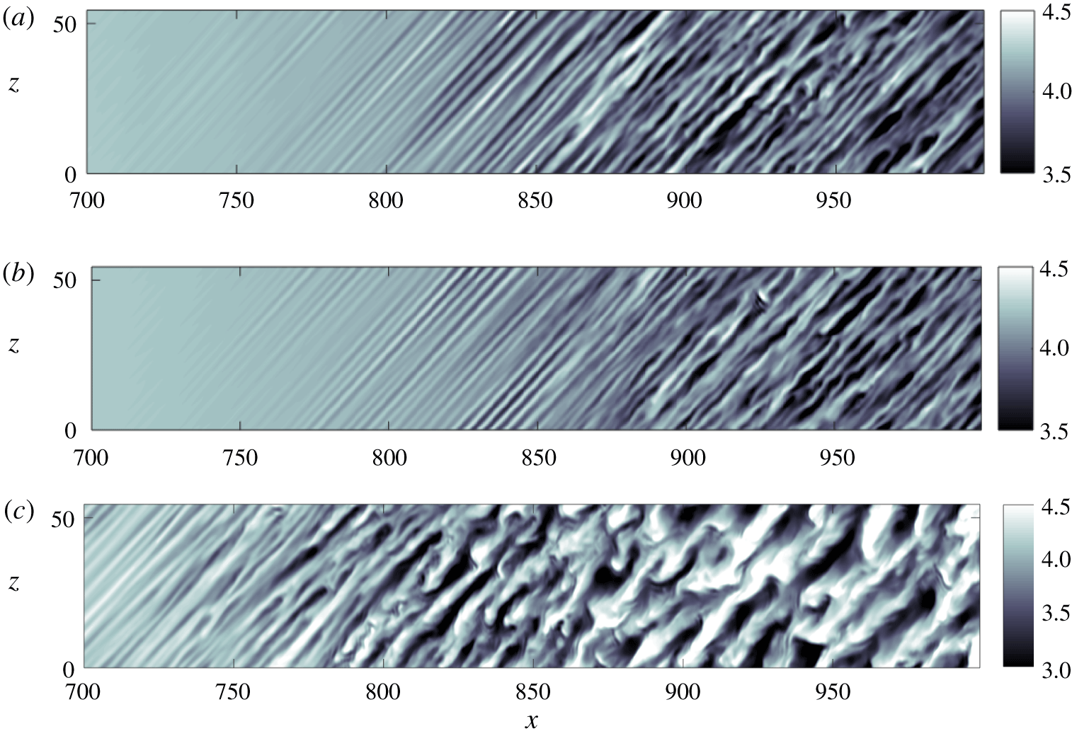
The effect of amplitude and disturbance type is shown in figure 14, where we plot temperature contours for each of cases 3–6, for which  $Re=5625$. It can be seen that streak breakdown is reached for the high-amplitude fast acoustic-wave case (case 4) at this higher Reynolds number, with the transition process occurring downstream of
 $x\approx 550$. At the low disturbance amplitude, in contrast, for both fast (case 3) and slow (case 5) acoustic waves, a 2-D wave pattern can be observed, as discussed for the lower Reynolds number case. For the fast-wave case, however, the 2-D waves appear more amplified than in the slow-wave case, which is a result of the resonance mechanism for mode F at the leading edge. Finally, the case of high-amplitude slow acoustic waves (case 6) in figure 14 shows the appearance of 3-D structures, consistent with the corresponding fast-wave case, but less amplified and with no breakdown.
In summary, these results for the unswept wedge demonstrate that the resonance mechanism occurring at the leading edge in the presence of free-stream fast acoustic waves induces a high amplification of mode F, which can have important implications in cases where nonlinear effects are not negligible. The resonant interaction between mode F and the fast acoustic waves at high free-stream amplitudes leads to significantly earlier boundary-layer transition, compared to the case of slow acoustic waves.
Instantaneous contour of the streamwise (tangential to the wall) velocity component ( $u_{t}$) along the grid line
 $j=10$ inside the boundary layer. Case 2,
 $A_{\infty }=5\times 10^{-2}$.

Instantaneous temperature ( $T$) contours along the grid line
 $j=10$ inside the boundary layer. (a) Case 3: fast acoustic waves,
 $A_{\infty }=5\times 10^{-3}$, (b) case 4: fast acoustic waves,
 $A_{\infty }=5\times 10^{-2}$, (c) case 5: slow acoustic waves,
 $A_{\infty }=5\times 10^{-3}$, (d) case 6: slow acoustic waves,
 $A_{\infty }=5\times 10^{-2}$.

For the specific case of hypersonic wind tunnels, it is known from previous studies, e.g. Duan et al. (Reference Duan, Choudhari and Wu2014), Wagner et al. (Reference Wagner, Schülein, Petervari, Hannemann, Ali, Cerminara and Sandham2018) and Cerminara et al. (Reference Cerminara, Durant, André, Sandham and Taylor2019), that slow acoustic waves are likely to be the most dominant acoustic disturbance radiated from the turbulent boundary layer on the nozzle wall. This does not mean, however, that fast modes are not of interest. Another relevant source of disturbances is represented by entropy spottiness that may come from the wind-tunnel reservoir. As the entropy waves, as well as the vorticity waves, show a receptivity mechanism similar to that of the fast acoustic waves, as described by Fedorov’s mechanism (Fedorov & Khokhlov Reference Fedorov and Khokhlov2001; Fedorov Reference Fedorov2011), and proved numerically by Ma & Zhong (Reference Ma and Zhong2005), an in-depth study of the breakdown mechanism associated with fast acoustic waves is relevant for these types of non-acoustic disturbances. Moreover, in agreement with several previous numerical studies, e.g. Ma & Zhong (Reference Ma and Zhong2003a), Balakumar (Reference Balakumar2009) and Egorov et al. (Reference Egorov, Sudakov and Fedorov2006), the present study shows that the fast mode, although stable, has growth factors higher than the slow mode in the leading-edge region (upstream of the Mack mode excitation). Furthermore, it is important to mention that fast acoustic waves may be important in other scenarios, e.g. in flight, where structure vibrations supplement the noise generated from turbulent boundary layers.
Fourier-transformed response of the  $x$-velocity component at the subharmonic frequency
 $f_{0}$ inside the boundary layer, along the
 $j=10$ grid line. Case 9,
 $A_{\infty }=5\times 10^{-3}$, slow waves.

4 Results for the swept wedge
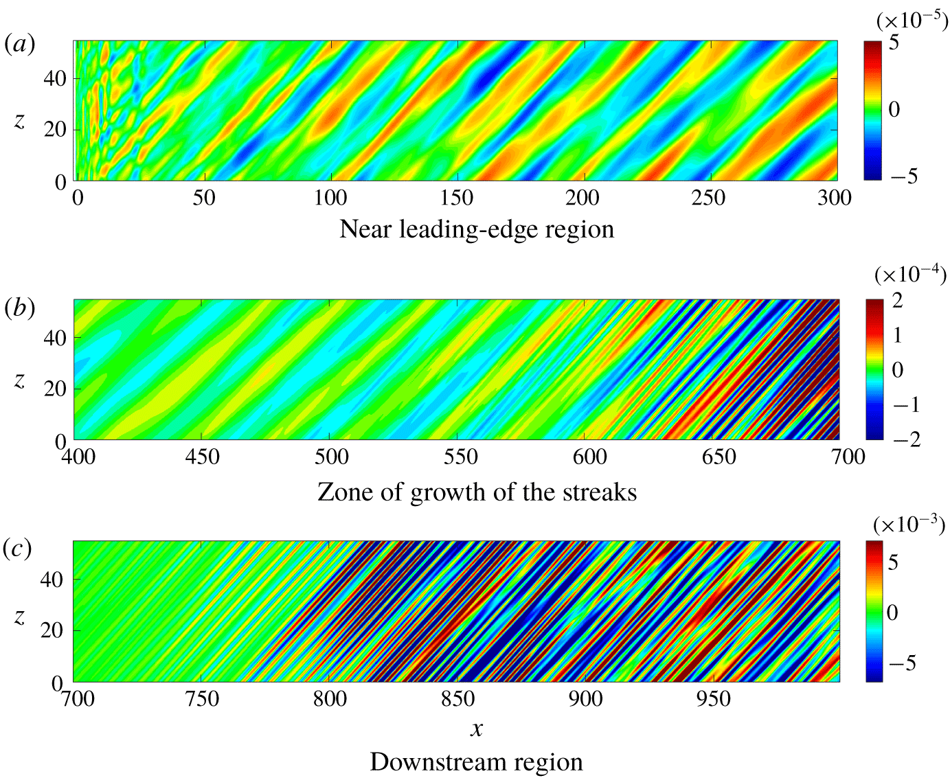
Results presented in this section refer to the swept wedge case at the higher Reynolds number ( $Re=5625$). An overview of the phenomena present in the simulations is provided by figure 15, which shows contours of the
 $x$-velocity fluctuation amplitudes in the wall-parallel plane at grid line
 $j=10$ in three different flow regions, namely near the leading edge, the growth zone of narrow streaks that are a peculiarity of this flow and the downstream region. The plots are shown for the (unforced) frequency
 $f_{0}=3.509\times 10^{-3}$, where the underlying physical processes are not hidden by the imposed forcing. After some evidence for leading-edge-parallel structures arising from a leading-edge receptivity mechanism for
 $x<25$, a cross-flow mode emerges, which is dominant over most of the wedge surface. For
 $x>550$, we then identify the formation of very narrow streaks with an order of magnitude higher spanwise wavenumber compared to the cross-flow mode. We start the investigation of these phenomena by showing numerical results, to present the transition scenario for fast and slow acoustic waves with different amplitude. Then, we use flow field data and 3-D LST results, obtained at different streamwise locations on the wedge surface, to study the boundary-layer instability and breakdown processes.
4.1 DNS results
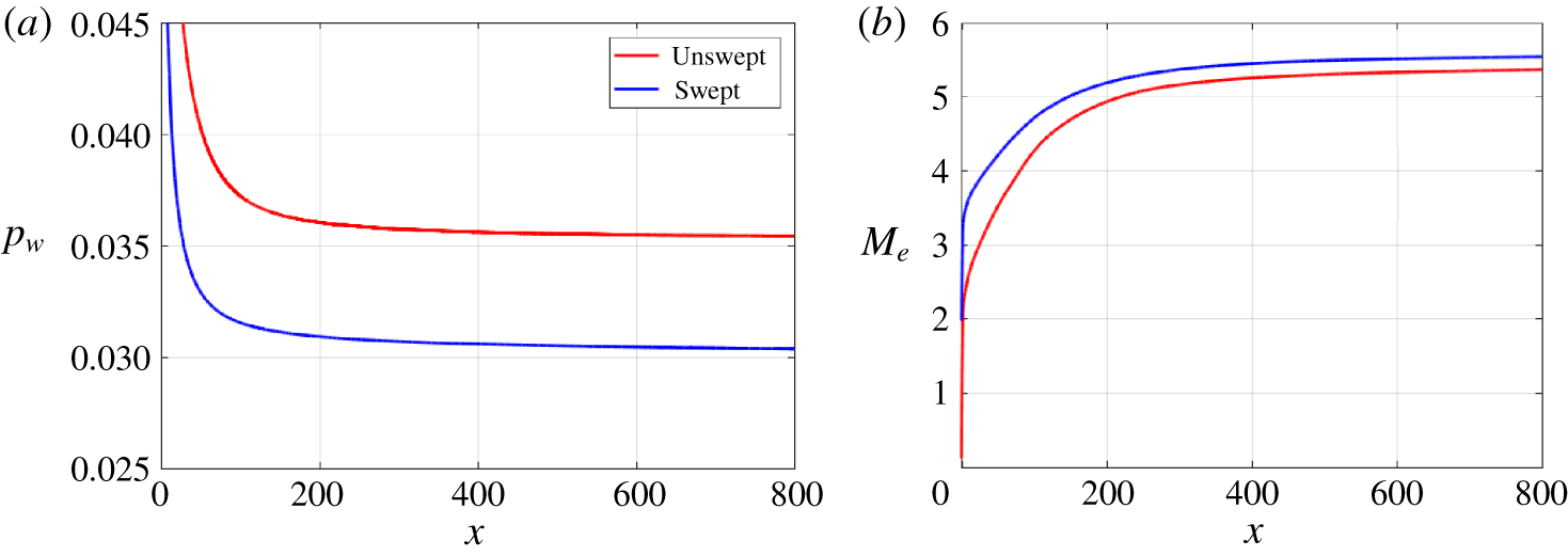
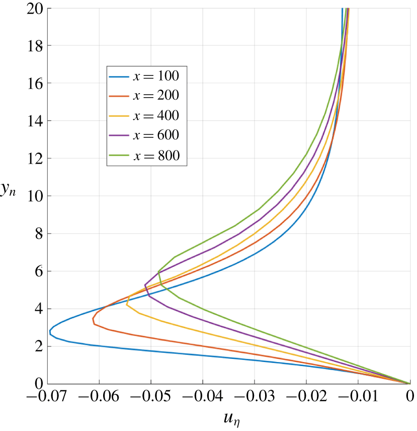
For the swept cases, pressure gradients normal to the free-stream direction lead to a laminar base flow that contains inflectional cross-flow boundary-layer profiles. Figure 16 shows the variation of the wall pressure and the Mach number at the edge of the boundary layer along the chordwise direction ( $x$), considering both the unswept and swept base flow. Due to the weaker shock wave induced by a non-zero sweep angle, the wall pressure is lower in the swept wedge case, while the Mach number at the boundary-layer outer edge is higher over the whole wedge length, compared to the unswept case. Figure 17 shows examples of inflectional cross-flow boundary-layer profiles at different distances from the leading edge. The coordinate directions for the cross-flow were defined in figure 4, with
 $u_{\unicode[STIX]{x1D702}}$ denoting the velocity in the cross-flow direction. Figure 18 shows a close up of the Mach number field in the leading-edge region, which highlights the shock stand-off distance as well as the very thin subsonic region around the circular leading-edge profile.
(a) Wall-pressure variation and (b) Mach number variation at the boundary-layer edge in the chordwise ( $x$) direction, for the unswept and swept base flows.

Cross-flow boundary-layer profiles at several distances from the leading edge.

Mean Mach number field in the leading-edge region.

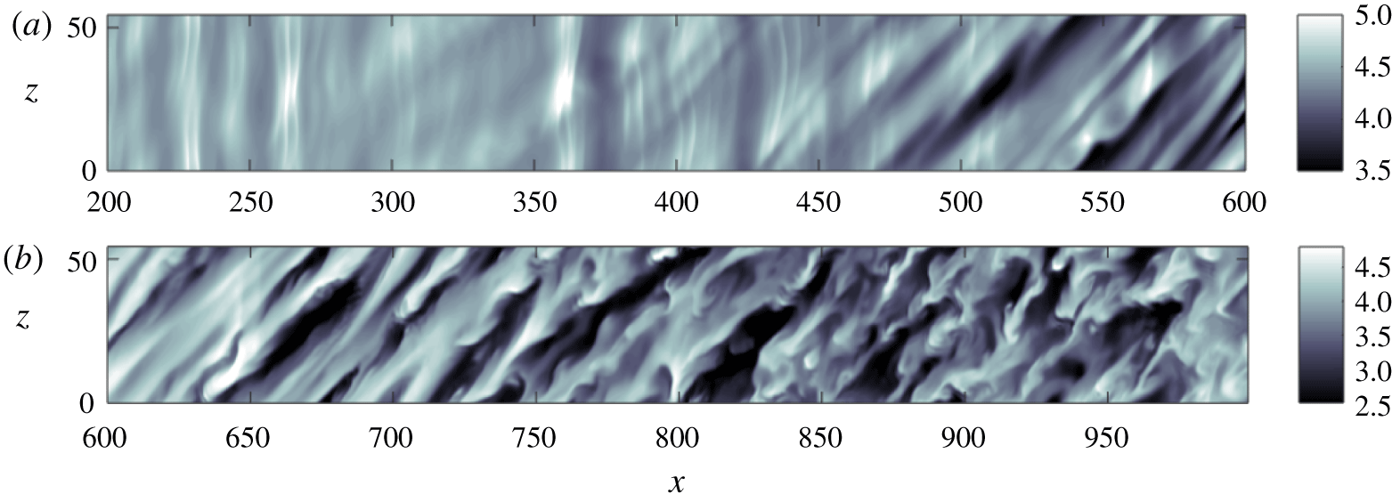
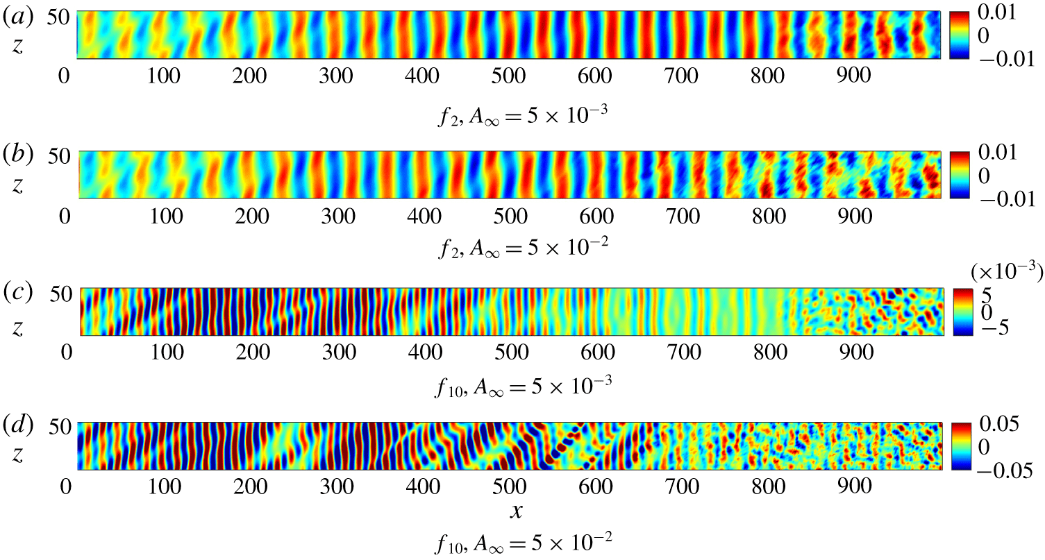
An overview of the transitional flow is provided by figures 19 and 20, showing contours of temperature inside the boundary layer for cases 7–10. The cases shown in figure 19 all have a similar breakdown mechanism, which appears more rapid in the high-amplitude slow-wave case. All the cases, even at the lower amplitude, show the start of nonlinear breakdown to turbulence. In each case, transition appears to be related to the formation and breakdown of streamwise-oriented streaks. The streaks are visible as elongated structures of alternate high and low temperature, corresponding respectively to low and high values of the streamwise velocity.
The case of fast acoustic waves at higher disturbance amplitude shown in figure 20 is different to the others in several aspects. First, this is the case where transition occurs at the earliest location, thus revealing that nonlinear effects related to the higher amplitudes are prevalent for fast acoustic waves. Secondly, this case shows the presence of spanwise-coherent structures up to  $x\approx 450$. This is consistent with the results obtained for the unswept case, in which it was shown that the resonance of the 2-D fast acoustic modes in the leading-edge region is a powerful mechanism of amplification of the internal waves, which can rapidly trigger transition at the higher amplitudes. A third noticeable difference of the fast-wave case at high amplitude is that the streamwise streaks have a much higher wavelength compared to the narrow streaks observed in the other cases. This is consistent with the presence of an unstable cross-flow mode.
Instantaneous temperature ( $T$) contours along the grid line
 $j=10$ inside the boundary layer. (a) Case 7: fast acoustic waves,
 $A_{\infty }=5\times 10^{-3}$, (b) case 9: slow acoustic waves,
 $A_{\infty }=5\times 10^{-3}$, (c) case 10: slow acoustic waves,
 $A_{\infty }=5\times 10^{-2}$.

Instantaneous temperature ( $T$) contours along the grid line
 $j=10$ inside the boundary layer. Case 8, fast acoustic waves,
 $A_{\infty }=5\times 10^{-2}$. (a) Near leading-edge region, (b) downstream region.

Real part of the Fourier-transformed wall-pressure fluctuations ( $p_{w}^{\prime }$) at the frequencies
 $f_{2}$ and
 $f_{10}$, at low (case 7) and high (case 8) amplitude. Fast acoustic waves.

Real part of the Fourier-transformed wall-pressure fluctuations ( $p_{w}^{\prime }$) at the frequencies
 $f_{2}$ and
 $f_{10}$, at low (case 9) and high (case 10) amplitude. Slow acoustic waves.

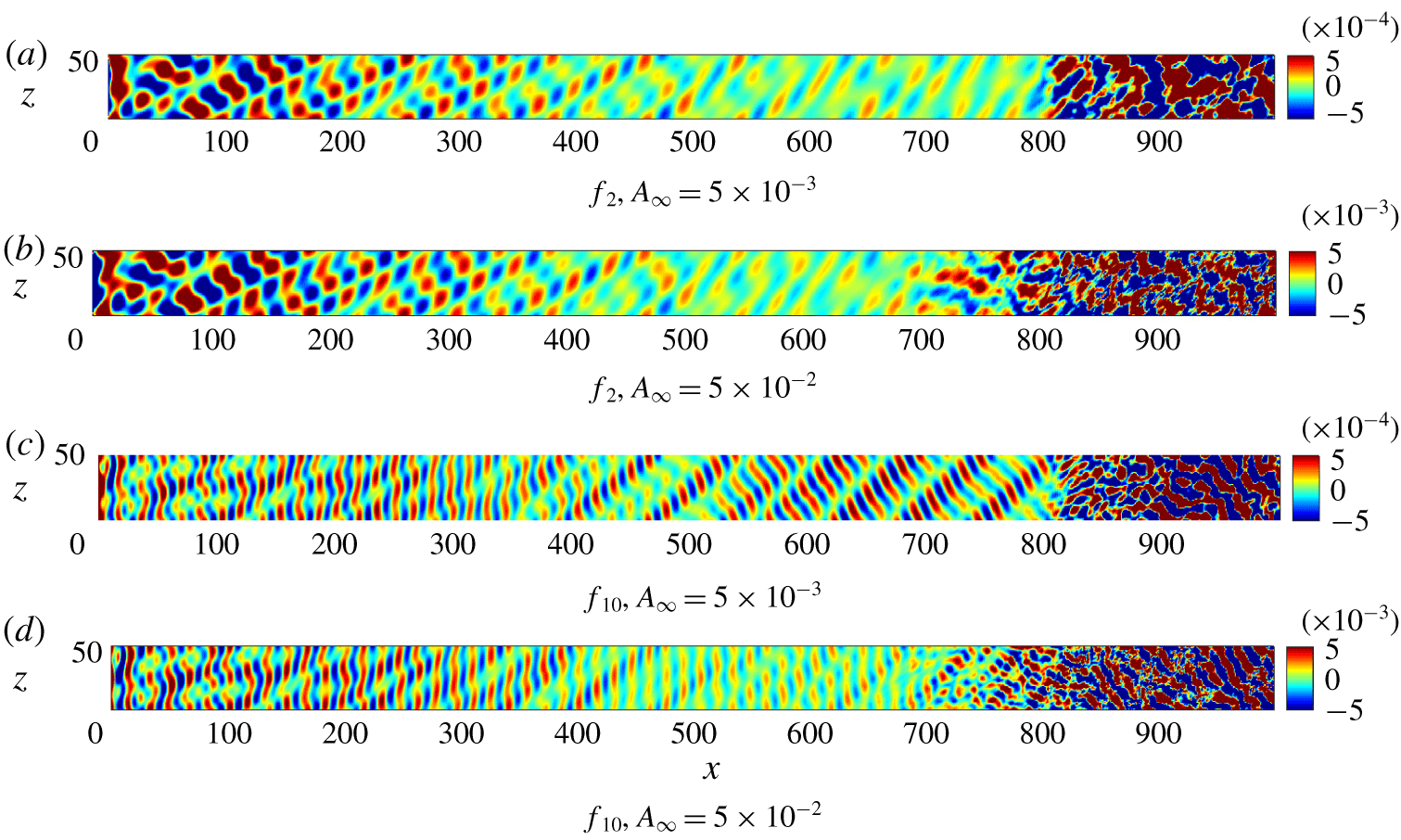
A first step towards the identification of the main wave modes involved in the receptivity process at different frequencies is made using a fast Fourier transform of the wall-pressure response, as was done in figures 10 and 11 in the previous section. Figures 21 and 22 show the Fourier-transformed pressure fluctuation amplitudes at the forcing frequencies  $f_{2}$ and
 $f_{10}$ (representative of the low- and high-frequency response) and at the different amplitudes, for fast and slow acoustic waves, respectively. The initial response to fast acoustic waves is characterised by a dominant 2-D wave pattern, for both frequencies and both amplitudes. This is a result of the same resonance mechanism between the forcing fast acoustic waves and the induced fast mode (or mode F) that was discussed in detail in § 3. At the higher frequency,
 $f_{10}$, the peak of the fast mode shifts closer to the leading edge, within
 $x=100{-}300$, whereas downstream of this region the amplitude decreases, consistent with the de-synchronisation of mode F. In the high-amplitude case, downstream of
 $x=400$, the 2-D mode is seen to be competing with another emerging structure that is aligned with the mean flow direction. As a result of this modulation, the wall response shows high amplitudes for a longer distance downstream, compared to the case with low free-stream disturbance amplitude. A similar structure is also present in the leading-edge region, seen more clearly at the higher frequency, but also present at the lower frequency.
In the case of slow acoustic-wave forcing, shown in figure 22, the 2-D mode does not play the same role as in the fast-wave case. At low frequencies a complex three-dimensional pattern appears in the leading-edge region, suggesting the presence of several oblique modes that can be more clearly distinguished further downstream. These low-frequency modes decay downstream, and do not appear to be directly responsible for the sudden breakdown to turbulence seen near  $x=800$. At the higher frequencies, the response near the leading edge shows a 2-D wave pattern that is strongly modulated by cross-flow-like modes, whereas further downstream oblique waves with higher spanwise wavenumber are clearly present.
These numerical results of the wall response at the different frequencies reveal the presence of at least three relevant modes that may play a determining role in the transition process. These modes consist of 2-D waves (wave fronts parallel to the leading edge), waves aligned in the mean flow ( $\unicode[STIX]{x1D709}$) direction (suggestive of cross-flow instabilities), and waves with wave fronts aligned in the cross-flow (
 $\unicode[STIX]{x1D702}$) direction. The type of the free-stream acoustic waves, either fast or slow, determines which of the above mentioned modes is dominant in a certain flow region. To further understand the flow behaviour we next use LST to determine the most relevant unstable modes in the boundary layer.
Temporal growth rate ( $\unicode[STIX]{x1D714}_{i}$) from linear stability analysis at different
 $x$ locations on the wedge.

4.2 Results from linear stability analysis
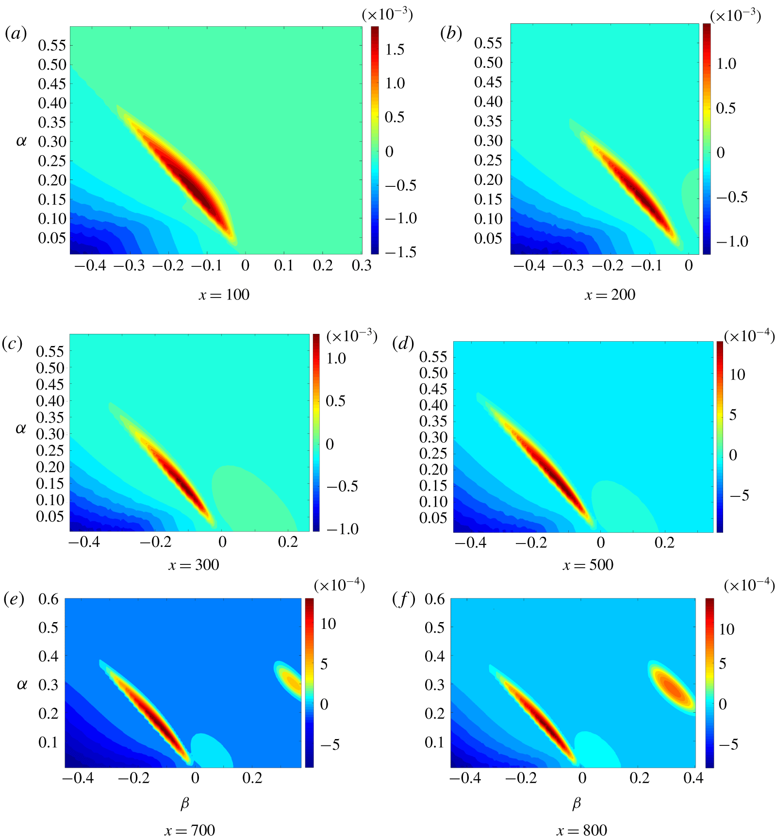
Profiles for analysis using LST are extracted from the computed solution for steady laminar flow over the swept wedge. Figure 23 shows contours of the temporal growth rate ( $\unicode[STIX]{x1D714}_{i}$) taken at different
 $x$-locations along the wedge, as well as at different
 $x$-wise and spanwise wavenumbers (
 $\unicode[STIX]{x1D6FC}$,
 $\unicode[STIX]{x1D6FD}$). With reference to figure 4, the wavenumbers
 $\unicode[STIX]{x1D6FC}$ and
 $\unicode[STIX]{x1D6FD}$ are the wavenumbers in the
 $xz$-reference system, i.e. with axes oriented in the chordwise and leading-edge directions. Hence, in this section, the wavenumber
 $\unicode[STIX]{x1D6FC}$ will be defined as the
 $x$-wise wavenumber (instead of streamwise wavenumber), to distinguish it from the wavenumber in the main flow (i.e. streamwise) direction. The ranges of
 $\unicode[STIX]{x1D6FC}$ and
 $\unicode[STIX]{x1D6FD}$ cover the free-stream forcing waves, for example the
 $x$-wise wavenumbers corresponding to the imposed frequency range are
 $\unicode[STIX]{x1D6FC}=0.126{-}0.353$ and
 $\unicode[STIX]{x1D6FC}=0.2{-}0.57$ for fast and slow acoustic waves, respectively. The corresponding forcing spanwise wavenumbers are
 $\unicode[STIX]{x1D6FD}=\pm 0.11$ (or alternatively
 $m=\pm 1$) and
 $\unicode[STIX]{x1D6FD}=\pm 0.22$ (
 $m=\pm 2$) for both fast and slow waves and at each forcing frequency. At all the considered locations (
 $x=100$, 200, 300, 500, 700, 800) the region of dominant instability (i.e. positive
 $\unicode[STIX]{x1D714}_{i}$) can be seen in figure 23 as the narrow elongated red regions with negative
 $\unicode[STIX]{x1D6FD}$. Within these regions, increasingly negative
 $\unicode[STIX]{x1D6FD}$ correspond to increasingly positive
 $\unicode[STIX]{x1D6FC}$ with approximately a constant ratio (
 $\unicode[STIX]{x1D6FD}/\unicode[STIX]{x1D6FC}\approx -0.83$, i.e.
 $\unicode[STIX]{x1D703}_{xz}\approx -40^{\circ }$), i.e. there is a constant orientation of the wave vector, which coincides with the local direction of the maximum cross-flow inside the boundary layer. The dominant unstable modes are travelling cross-flow waves, which are known to be associated with free-stream disturbances (Li et al. Reference Li, Choudhari, Duan and Chang2014, Reference Li, Choudhari, Paredes and Duan2016; Bartkowicz et al. Reference Bartkowicz, Subbareddy and Candler2010) at low frequencies, such as those imposed in our simulations (
 $f_{1}^{\ast }=12.6~\text{kHz}$,
 $f_{10}^{\ast }=35.3~\text{kHz}$). The phase speed of the most unstable cross-flow mode from LST, taken in the direction of the wave vector (
 $c_{ph}=\unicode[STIX]{x1D714}_{r}/\sqrt{\unicode[STIX]{x1D6FC}^{2}+\unicode[STIX]{x1D6FD}^{2}}$), is
 $c_{ph}=0.057$ at
 $x=400$, and
 $c_{ph}=0.058$ at
 $x=500$, and the corresponding wavenumbers are
 $\unicode[STIX]{x1D6FC}=0.138$ and
 $\unicode[STIX]{x1D6FD}=-0.11$. The spanwise wavenumber coincides with the imposed
 $m=1$ wavenumber, whereas the
 $x$-wise wavenumber approximately corresponds to the lowest imposed
 $\unicode[STIX]{x1D6FC}$ for fast acoustic waves. The most unstable cross-flow waves are travelling waves with a significantly lower phase speed compared to the imposed free-stream fast and slow acoustic waves. The corresponding frequency is
 $f=0.0016$, which is an order of magnitude lower than our minimum imposed non-dimensional frequency (
 $f_{1}=0.0175$). In dimensional units, the frequency of the most unstable cross-flow mode, considering a reference nose radius of
 $R^{\ast }=1.2$ mm, is
 $f_{mode}^{\ast }=1.15~\text{kHz}$, representing a subharmonic of the free-stream forcing.
For  $x>200$ the LST results show the presence of other instabilities. The first to emerge is located at the low wavenumbers (
 $\unicode[STIX]{x1D6FC}<0.2$), peaking at a small positive value of
 $\unicode[STIX]{x1D6FD}$, for example peaking at
 $\unicode[STIX]{x1D6FD}=0.1$,
 $\unicode[STIX]{x1D6FC}=0.1$ at
 $x=300$. This corresponds to a first mode instability (Reshotko Reference Reshotko1976), with a wave orientation perpendicular to the cross-flow mode. The region of first mode instability is present at all the other locations downstream of
 $x=200$ along the wedge, but the associated growth rates are very low.
At the location  $x=700$ another unstable mode appears, with a growth rate lower than the dominant cross-flow mode, but higher than the first mode growth rate. This mode is a higher-frequency mode (i.e. higher wavenumber
 $\unicode[STIX]{x1D6FC}$), and corresponds to higher positive
 $\unicode[STIX]{x1D6FD}$ values. The values of
 $\unicode[STIX]{x1D6FC}$ and
 $\unicode[STIX]{x1D6FD}$ are approximately equal within this high-frequency instability region, which means that these modes are inclined of an angle of about
 $45^{\circ }$ with respect to the
 $x$-axis, i.e. they are effectively 2-D modes in the mean flow reference system (rotated by the sweep angle with respect to the geometry reference system), and correspond to 2-D second modes (Mack Reference Mack1984). The phase speed of the modes in this region is about
 $c_{ph}\approx 0.85{-}0.87$, which is consistent with the phase speed associated with the Mack mode (Reshotko Reference Reshotko1976; Ma & Zhong Reference Ma and Zhong2005; Zhong & Wang Reference Zhong and Wang2012). The corresponding non-dimensional frequency associated with these modes is about
 $f=0.06$, which in for a reference nose radius of 1.2 mm would give a dimensional frequency of 43 kHz. This would explain the generally low growth rates (
 $\unicode[STIX]{x1D714}_{i}$ values) of the second mode seen here. The experiments about the second instability mode are usually performed over smaller nose radii, e.g. 0.1 mm (Estorf et al. Reference Estorf, Radespiel, Schneider, Johnson and Hein2008; Wagner et al. Reference Wagner, Schülein, Petervari, Hannemann, Ali, Cerminara and Sandham2018), as it is known that a sharper leading edge provides higher growth rates for the Mack mode, as was shown for example from Malik & Balakumar (Reference Malik and Balakumar2007) for a flat plate with different blunt nose radii. For a nose radius lower than 0.5 mm, i.e. a sharp leading edge, this non-dimensional frequency of 0.06 would correspond to a dimensional frequencies
 $f^{\ast }>100~\text{kHz}$, which then would include the usual frequency range (100–300 kHz) associated with second mode experiments (Estorf et al. Reference Estorf, Radespiel, Schneider, Johnson and Hein2008) in hypersonic wind tunnels.
The overall growth in amplitude of an instability wave can be quantified using the  $N$-factor (Crouch & Ng Reference Crouch and Ng2000), defined by
 $$\begin{eqnarray}N=\log \left(\frac{A(x)}{A(x_{0})}\right)=\int _{x_{0}}^{x}-\unicode[STIX]{x1D6FC}_{i}(x)\,\text{d}x,\end{eqnarray}$$
in which the spatial growth rate  $-\unicode[STIX]{x1D6FC}_{i}$ is approximated from
 $\unicode[STIX]{x1D714}_{i}$ using Gaster’s relation (Gaster Reference Gaster1962), which can be expressed as
 $$\begin{eqnarray}\frac{\unicode[STIX]{x1D714}_{i}^{T}}{\unicode[STIX]{x1D6FC}_{i}^{S}}=-\frac{\unicode[STIX]{x2202}\unicode[STIX]{x1D714}_{r}}{\unicode[STIX]{x2202}\unicode[STIX]{x1D6FC}_{r}}=-c_{g}.\end{eqnarray}$$
In the above equation the superscripts  $T$ and
 $S$ stand for temporal and spatial, respectively, whereas the term
 $c_{g}$ is known as the group velocity. Figure 24 shows the computed
 $N$-factors for the most unstable cross-flow mode from LST compared with the
 $N$-factors of different Mack modes taken in their unstable region. A logarithmic scale is used along the
 $N$ axis in order to show the difference between the
 $N$-factor levels of the cross-flow and Mack modes. As can be seen, the amplification (
 $N$) factors of the Mack modes resulting from the LST, shown in a form to outline part of the envelope of maximum amplification factors in figure 24, are very small compared to those of the cross-flow mode, thus suggesting that the unstable Mack modes are not responsible for transition. Nor is the unstable first mode expected to be important, since its growth rate is an order of magnitude lower than the cross-flow mode.
The  $N$-factors of the most unstable cross-flow mode and Mack modes at different
 $\unicode[STIX]{x1D6FC}$ and
 $\unicode[STIX]{x1D6FD}$ wavenumbers.

Comparison of temporal and spatial approaches. Assessment of Gaster’s transform.

The validity of Gaster’s relation for the considered flow is assessed by direct comparison between the approximated spatial growth rates ( $\unicode[STIX]{x1D6FC}_{i}$) obtained from Gaster’s relation and those obtained by a spatial linear stability analysis. The comparison has been made at two
 $x$ locations, namely
 $x=400$ and
 $x=500$, in which the temporal LST results indicate the presence of cross-flow instabilities. At both locations, the most unstable mode has been considered, as Gaster’s relation is known to be valid only for modes with growth rate close to zero. The results of this comparison are tabulated in table 4. Results for both temporal and spatial approaches are shown at both the locations. The most unstable mode found at these locations is a cross-flow mode with
 $x$-wise and
 $z$-wise wavenumbers
 $\unicode[STIX]{x1D6FC}=0.138$ and
 $\unicode[STIX]{x1D6FD}=-0.111$. The corresponding wavenumbers in the reference system aligned with the free-stream flow direction (streamwise,
 $\unicode[STIX]{x1D709}$) and the cross-flow (
 $\unicode[STIX]{x1D702}$) direction are
 $\unicode[STIX]{x1D6FC}_{\unicode[STIX]{x1D709}}=0.019$ and
 $\unicode[STIX]{x1D6FD}_{\unicode[STIX]{x1D702}}=-0.1761$. In table 4 the streamwise wavenumber in the flow reference system is given, whose real part is indicated as
 $\unicode[STIX]{x1D6FC}_{\unicode[STIX]{x1D709},r}$. The term
 $\unicode[STIX]{x1D714}_{r}$ represents the real part of the frequency obtained from the temporal approach, which is used as input in the spatial approach. The streamwise phase speed
 $c_{ph}$ (i.e. the phase speed of the mode in the
 $\unicode[STIX]{x1D709}$ direction) represents the ratio between
 $\unicode[STIX]{x1D714}_{r}$ and
 $\unicode[STIX]{x1D6FC}_{\unicode[STIX]{x1D709},r}$, and is an output in both the temporal and spatial approaches. The spatial growth rate
 $\unicode[STIX]{x1D6FC}_{i}^{S}$ is the output of the spatial analysis and is approximated by (4.2) using the temporal approach. As can be seen, the spatial growth rates from the spatial LST and Gaster’s transform are very similar at both the locations. The relative error between the two values is 1.9 % at
 $x=400$ and 1.6 % at
 $x=500$. These results, obtained for the most unstable mode, confirm the validity of Gaster’s transform as well as the suitability of the temporal LST for the present case.
No other modes have been found in LST. In particular no linear instability modes were found for the chordwise and spanwise wavenumbers of the narrow streaks that are seen in the flow visualisations in figure 19. Thus these features are not associated with a primary flow instability. Nor are they obviously a secondary instability of a finite-amplitude cross-flow mode. The results of the cross-flow mode are streamwise vortices and lifted streaks that would be expected to support well-known secondary streak instabilities, for example of the sinuous or varicose type (Kohama Reference Kohama1987; Andersson et al. Reference Andersson, Brandt, Bottaro and Henningson2001; Li et al. Reference Li, Choudhari, Duan and Chang2014). In order to understand the final stages of transition we need find the origin and growth mechanism of the narrow streaky flow features. This will be the subject of the following section.
4.3 Streak-induced breakdown mechanism
The wavenumbers associated with the narrow streaks are approximately one order of magnitude higher than the forced wavenumbers of the free-stream noise. They are not the result of a local primary flow instability and we are not aware of any published secondary instability mechanisms that lead to streaks with much higher spanwise wavenumber, but they are oriented in the same direction as the primary instability. Understanding the origin and growth of the mode associated with the narrow streaks requires a more in-depth analysis of the DNS results in the upstream region. Figure 25 shows 3-D views of the  $u^{\prime }$ and
 $v^{\prime }$ velocity components in the flow region where the narrow streaky structures appear and rapidly grow. Figure 25(b) gives a good impression of the underlying wave system in the region
 $x=480{-}620$. In this region there is a change taking place from structures parallel to the leading edge towards more oblique structures. The corresponding
 $u$-component of the fluctuations (figure 25a) shows very pronounced narrow streaks that are present even at the start of this image and hence do not appear to be connected to the change in orientation of the underlying waves. Nor is a numerical source likely. A lack of flow resolution with a high-order code of the type used here gives oscillations with wavelength twice the grid spacing when the flow is under-resolved. However, with approximately seven wavelengths across the span and 100 grid points, we already have better than 12 points per wavelength of the narrow streaks and no evidence of any under-resolution of the local flow features.
Surface views of the chordwise and wall-normal velocity component fluctuations. Case 9.

To pin down the origin of the narrow streaks, figure 26 shows the temperature contours in the region  $x=300{-}750$ inside the boundary layer at different
 $j$ grid lines. Downstream of
 $x=500$, narrow streaks (
 $m\approx 7{-}9$) start to be evident, and downstream of
 $x=650$ their amplitude reaches very high levels. The streaks form in a limited region within the boundary layer that is close to the maximum cross-flow velocity. For example
 $j=15$ corresponds to
 $y_{n}\approx 5$ at
 $x=600$ in figure 17.
Temperature fluctuation contours inside the boundary layer, at different  $j$-grid lines. Case 9.

The origin of the localised region in  $y$ in which the
 $m=O(10)$ mode develops can be deduced from figure 27, showing cross-sections of the streamwise vorticity fluctuations at two different
 $x$ stations. At the upstream station,
 $x=400$, the vorticity shows two narrow layers of positive and negative vorticity, one on top of the other. The location at
 $y=32$, corresponding to a wall-normal distance of
 $y_{n}=3$, locates this feature at the inflection point of the cross-flow profiles shown in figure 17. At
 $x=525$ spanwise oscillations have started to form and it is clearly the roll-up of the streamwise vorticity that leads, via a lift-up mechanism, to the narrow velocity streaks seen in figure 25. If we take the thickness of the layer as approximately 2 and the velocity difference as 0.05 from the cross-flow profiles on figure 17, the local shear layer Reynolds number is approximately 500, which is sufficient for the roll-up of the shear layer to develop via an essentially inviscid mechanism. Figure 28 shows the eigenfunctions of streamwise, vertical and cross-flow velocity components as well as temperature of the most unstable cross-flow mode (
 $\unicode[STIX]{x1D6FC}=0.138$,
 $\unicode[STIX]{x1D6FD}=-0.11$), from LST at the location
 $x=400$. As can be seen, the cross-flow mode fluctuations peak at approximately the same location of the thin vorticity fluctuation layer seen in figure 27 (the location of the inflection point of the cross-flow profile), i.e.
 $y_{n}\approx 3{-}4$, thus confirming that the thin vorticity layer is a feature associated with the cross-flow instability. A further confirmation is given by figure 28(b), which depicts the profile of the streamwise vorticity fluctuations computed from the eigenfunctions of the velocity components in figure 28(a). The vorticity profile shows a narrow layer of oscillations, with maximum located at the peak location of the eigenfunctions, consistent with the narrow vorticity fluctuation layer seen in figure 27.
Cross-sections of the streamwise vorticity fluctuations ( $\unicode[STIX]{x1D714}_{\unicode[STIX]{x1D709}}^{\prime }$) at different
 $x$ locations. Case 9.

Eigenfunctions of the cross-flow instability mode and corresponding vorticity fluctuations at the  $x=400$ location. Case 9.

Having identified the  $m=O(10)$, corresponding to
 $\unicode[STIX]{x1D6FD}=O(1)$, mode as responsible for the roll-up of the thin vorticity layer associated with the cross-flow mode, the final part of the puzzle is to find its origin, since this mode is not present in the free-stream forcing. By performing a fast Fourier transform in space at different
 $x$ stations close to the leading edge, it is possible to verify which higher wavenumbers are generated, and their relative amplitude. Figure 29 shows the spanwise wavenumber spectrum of the
 $x$-velocity fluctuation amplitudes inside the boundary layer (along the
 $j=10$ grid line). The spatial fast Fourier transform has been performed in the spanwise direction for the Fourier-transformed (in time) signal at the fundamental frequency
 $f_{0}$. There is also a pronounced amplification of a higher (unforced) wavenumber,
 $m=6$, which decays at higher distances from the leading edge (
 $x=250$, 500), and then increases again further downstream (
 $x=600$). Other lower peaks are observed at the higher distances for increasing wavenumbers.
Spectrum of the Fourier-transformed amplitudes of the  $x$-velocity fluctuations along the
 $j=10$ grid lines, in the domain of the spanwise wavenumbers, at different
 $x$ positions. The spectrum has been computed at the frequency
 $f_{0}$. Case 9.

Streamwise distribution of the Fourier-transformed  $x$-velocity fluctuations, along the
 $j=10$ grid lines, at the frequency
 $f_{0}$ and at high spanwise wavenumbers. Case 9.

The wavenumber  $m=11$ is present at a low-amplitude peak at the early location
 $x=20$, suggesting that it forms inside the boundary layer near the leading edge. The frequency of the most unstable cross-flow mode (
 $f=0.0016$) is half the fundamental frequency
 $f_{0}$ of our simulations. Thus, the closest frequencies to the frequency of the most unstable mode are those most responsible for the growth of the
 $m=O(10)$ modes. Due to limited computational resources, we are not able to process the
 $m=O(10)$ modes at the low frequency of the most unstable mode, but only at the lowest frequency we can extract from the numerical results, i.e. the fundamental frequency
 $f_{0}$, for which
 $m=11$ is found to be the dominant high wavenumber mode, as seen in figure 29. The spatial variation of the
 $m=6$ and
 $m=11$ modes is shown on figure 30. The initial amplification at the leading edge is followed by a decay after which the amplitude of the modes grows in the region
 $x=350{-}500$, followed by a more pronounced growth downstream of
 $x=500$, where the streaks are seen to grow. In this latter region, the growth of the mode
 $\unicode[STIX]{x1D6FD}_{11}$ is more rapid than that of
 $m=6$, which causes
 $m=11$ to become the dominant wavenumber associated with the streaks. Thus, the spectrum of figure 29 shows that higher wavenumbers are generated in the early leading-edge region. The growth of the narrow streaks appears to be due to a transient growth mechanism associated with the roll-up of the narrow streamwise vorticity layer (as previously described), whose length scale is comparable with the wavelength of the narrow streaks.
Sketch of the wave system characterising the shock layer region.

Sketch of wave scattering at the leading edge on an  $xy$-plane.

The generation mechanism of the smaller wavelengths at the leading edge can be discussed with reference to the sketches shown in figures 31 and 32, which illustrate some potentially relevant phenomena involving the acoustic waves in the shock layer. Figure 31 shows a top view of the  $xz$-plane at the location of the minimum shock stand-off distance, indicated by
 $\unicode[STIX]{x1D6E5}=0.55$, whereas figure 32 shows the scattering of the incident acoustic waves from the rounded leading edge (in a
 $xy$-plane). Due to the presence of the shock, there is a complex wave system in the shock layer, characterised by wave refraction, reflection and scattering from the leading edge. The incident free-stream waves are refracted downstream of the shock, with mechanisms described in McKenzie & Westphal (Reference McKenzie and Westphal1968), and propagate towards the wall with different orientations. The leading edge, in turn, can reflect the waves back to the shock (Cerminara & Sandham Reference Cerminara and Sandham2017) and scatter the waves in all directions. If we consider the multiple reflection process, the shock layer can be seen as a wave guide of thickness equal to the stand-off distance, which then promotes the formation of waves with wavelength comparable to the wave guide thickness. The scattering mechanism is particularly sensitive to the surface radius of curvature (in this case the wedge nose radius), and is more effective when a large difference between the wavelength of the incident waves and the body radius of curvature exists, which leads to the generation of scattered waves with wavelength comparable with the nose radius. This (speculative, but in our view plausible) wavelength and frequency conversion process would result in the generation of waves with significantly smaller wavelength compared to the wavelengths imposed in the free stream, as observed for example in figure 15(a) and warrants further investigation.
5 Conclusion
A set of ten direct numerical simulations have been performed for a Mach 6 flow over a wedge in an unswept and a swept ( $45^{\circ }$ sweep angle) configuration, for different types of free-stream acoustic waves, i.e. fast and slow waves, and different amplitudes, orientations and frequencies of the forcing. The objective is to investigate the physical mechanism of receptivity at the leading edge and the associated mechanisms of breakdown and transition in several scenarios. A circular leading edge is considered, where a well-known wavelength conversion mechanism broadens the wavelength spectrum of our imposed disturbances, generating different wavelengths, which play an important role in the transition process. By studying the complete receptivity transition process starting from free-stream disturbances over a body with a resolved leading edge, we expect to find new important features of the transition mechanism that are poorly visible or not measurable in transition experiments, or that are not captured in other typical numerical studies in which either (i) disturbances are directly imposed within the boundary layer, (ii) the leading edge is not included in the computational domain or (iii) only the early leading-edge receptivity to free-stream waves is studied. Linear stability analyses have been performed in support of the numerical simulations, to identify the local linear instabilities that are present in the boundary layer at the different flow conditions.
The study is initially performed for the unswept wedge case, at two Reynolds numbers based on the nose radius. A linear stability analysis of the base flow has assessed the well-known Fedorov receptivity mechanism at the leading edge to fast and slow acoustic waves, revealing the presence of the fast mode (mode F), the slow mode (mode S), and the Mack mode, as well as the wavelength exchange mechanism between mode F and mode S at their synchronisation point. The numerical simulations have confirmed the presence of a strong amplification of mode F at the leading edge, due to a resonance mechanism with the free-stream fast acoustic mode, as well as a modulation process taking place in the decay region of mode F, between different competing modes, including the external forcing and the excited slow mode in this region. Moreover, further downstream a second resonance mechanism with the fast acoustic waves is captured, with excitation of mode F II (using Zhong’s notation). The results from LST and DNS agree qualitatively very well with the reference theoretical studies of Fedorov, and the reference numerical studies of Zhong, when low amplitude disturbances are considered. When high-amplitude disturbances are imposed in the free stream, the numerical results show that the picture of the generated instabilities shifts significantly from the linear case, and the transition mechanism is significantly different for fast and slow acoustic waves. In particular, it is found that the high disturbance amplification induced from the resonance mechanism for the fast mode at the leading edge leads to nonlinear generation of an instability mode corresponding to streamwise streaks, which at a higher Reynolds number grow rapidly and break down. For high amplitude disturbances, fast acoustic waves induce an earlier transition process compared to slow acoustic waves.
The swept wedge case shows in general more complex features compared to the unswept case, due to the additional role played by cross-flow instabilities in the leading-edge region. Linear stability analyses show the presence of travelling cross-flow instabilities and other modes pertaining to the classes of first and second mode instabilities, which have very different growth rates and appear at different distances from the leading edge. The cross-flow instability represents the dominant instability mode over the whole length of the wedge. Consistent with the unswept wedge case, earlier bypass transition is reached when high-amplitude fast acoustic waves are considered, as a result of the initial disturbance amplification induced by the resonance mechanism for the fast mode at the leading edge. In this case, this mechanism provides a nonlinear destabilisation of the primary cross-flow instability waves generating in the leading-edge region, followed by rapid growth and breakdown. The process that leads to breakdown in all the other cases show different features to the high-amplitude fast-wave case. In particular, very narrow streaks oriented in the streamwise direction are observed, which are aligned with the primary cross-flow instability waves, and show a very rapid growth leading to streak breakdown, with the appearance of secondary streak instabilities.
An in-depth study of the origin and growth mechanism of these structures has confirmed that the narrow streamwise streaks are associated with the presence of high spanwise wavenumber (an order of magnitude higher than the primary cross-flow mode) modes,  $m=O(10)$, that are generated at the leading edge, as well as the presence of a narrow streamwise vorticity fluctuation layer located near the inflection point of the cross-flow boundary-layer profiles, whose length scale is comparable with the wavelength of the
 $m=O(10)$ modes. The narrow vorticity layer has been shown to be generated by the primary cross-flow instabilities, and the growth of the high wavenumber modes has been found to be associated with the lowest fundamental frequency, which is an unstable cross-flow mode. A transient growth mechanism has been found to be the source of the
 $m=O(10)$ mode growth, occurring through destabilisation and roll-up of the narrow vorticity layer. The source of the
 $m=O(10)$ modes in the leading-edge region is proposed as a mechanism of wave refraction, scattering and wall–shock–wall reflection occurring at the leading edge within the shock layer, and influenced by the very small length scale of the shock stand-off distance.
The present results provide new insights into the complex leading-edge receptivity transition mechanism with free-stream acoustic noise in hypersonic flows. As part of this, a plausible wavelength-conversion mechanism has been conjectured to explain the presence of disturbance wavelengths significantly shorter than those comprising the free-stream forcing. A more detailed investigation of this process should be undertaken, as this may be a missing piece of the overall transition mechanism.
Acknowledgements
The authors would like to acknowledge MBDA UK Limited for supporting the PhD project of the first author, and Dr N. J. Taylor for many useful discussions. Computer time on the UK National Supercomputing Service (ARCHER) was provided by the UK Turbulence Consortium (UKTC) under EPSRC (Engineering and Physical Sciences Research Council) grant no. EP/L000261/1. Finally, support is gratefully acknowledged from EPSRC under the grant no. EP/J016381/2 ‘Thermal and Reactive Flow Simulation on High-End Computers’ for additional computer time.
Declaration of interests
The authors report no conflict of interest.