‘I soon understood that there was little hope of developing a pure, closed theory, and, because of absence of such a theory, the investigation must be based on hypotheses obtained on processing experimental data’. [Kolmogorov, quoted by A. Tsinober]
1 Introduction
The first lesson I learned as a graduate student is that there is no official definition of turbulence. According to consensual observations, turbulence is a state of fluids characterized by swirling motions. Such motions are observed in a variety of phenomena, covering a wide range of scales, from the centimetre tap water vortex to
 $10^{2}$
km size hurricanes or
 $10^{4}$
light year galaxies. The building of a comprehensive theory of turbulence, allowing understanding and prediction of these phenomena, is therefore a long-standing issue. The situation of turbulence with respect to other outstanding problems in physics, such as the unification of gravity and quantum mechanics, is paradoxical. Contrary to the other problems, the constitutive equations governing the dynamics of turbulent flows are well-known. They are the incompressible Navier–Stokes equations (INSE) for unstratified fluids:
 $$\begin{eqnarray}\displaystyle & \displaystyle \unicode[STIX]{x2202}_{t}u_{i}+u_{j}\unicode[STIX]{x2202}_{j}u_{i}=-\frac{1}{\unicode[STIX]{x1D70C}}\unicode[STIX]{x2202}_{i}p+\unicode[STIX]{x1D708}\unicode[STIX]{x2202}_{j}\unicode[STIX]{x2202}_{j}u_{i}+f_{i}, & \displaystyle\end{eqnarray}$$
 $$\begin{eqnarray}\displaystyle & \displaystyle \unicode[STIX]{x2202}_{j}u_{j}=0, & \displaystyle\end{eqnarray}$$
where
 $u_{i}$
is the d-dimensional velocity field,
 $p$
the kinematic pressure,
 $\unicode[STIX]{x1D70C}$
the (constant) density,
 $f_{i}$
is the forcing and
 $\unicode[STIX]{x1D708}$
the molecular viscosity. Since Reynolds’ pioneering work, we know that after a proper rescaling of the equations by
 $L$
and
 $U$
, some characteristic length and velocity, the INSE only depend on one parameter, the Reynolds number
 $Re=LU/\unicode[STIX]{x1D708}$
.
Equipped with a set of equations depending only of one parameter, we should be in the most favourable situation to build a theory of turbulence – at least, that is often what my colleagues in quantum mechanics seem to think. When confronted with this question, I always give the same answer, which is probably the second lesson I learned from my turbulence classes: the INSE are nonlinear partial differential equations, and they have been resisting mathematical and analytical treatments for almost two centuries: (i) it is still not known whether their solutions with finite energy remain regular for all time – this is the subject of the Clay prize – and (ii) very few analytical solutions exists. Until the first half of the 20th century, before the advent of computers, any theory of turbulence could therefore only be based on hypotheses derived from observations or experimental data, as noted by Kolmogorov. Using a minimal set of such hypotheses, he was able in 1941 to construct a simple theory of turbulence based on the concept of energy cascade. Most of the present models or theories of turbulence are based on the Kolmogorov picture. It appears to describe successfully the large-scale structure of many turbulent flows encountered in practical situations such as aeronautics, industry, meteorology or astrophysics, but becomes increasingly inaccurate when going down the scales. This is problematic for the modelling of all processes that depend on small scales of turbulence, such as combustion instabilities, droplet atomization in industrial burners or cloud formation.
We now have powerful computers, insist my quantum physicist colleagues. Why not abandon any modelling and turn to direct numerical simulation (DNS) of turbulent flows using the INSE? My reply to this is of course that DNS implies discretizing the equations in space and time, i.e. choosing an appropriate time and space resolution. For this, we still need a good model of turbulence. If we use Kolmogorov theory, we find that to simulate a flow of scale
 $L$
and velocity
 $U$
at a given Reynolds number
 $Re$
, the resolutions in space and time should be
 $\unicode[STIX]{x0394}x\sim LRe^{-3/4}$
and
 $\unicode[STIX]{x0394}t\sim (L/U)Re^{-1/2}$
. The number of nodes
 $N$
to simulate then scales like
 $Re^{9/4}$
and the number of time steps to reach a time
 $T=L/U$
is
 $Re^{1/2}$
, making the computational burden
 $O(Re^{11/4})$
to simulate the flow over such a period. For any aeronautical, geophysical or astrophysical application, this exceeds by far the capabilities of the most powerful computers. It seems that, for the time being, we still are in need of a theory of turbulence that goes beyond the Kolmogorov picture so as to be able to handle better the small scales of turbulence and provide us with as sharp as possible bounds on the time and space discretization of DNS.
These issues have been at the heart of my research for over thirty years. Thanks to general scientific progress, we now have better clues regarding mathematical or analytical properties of INSE with respect to the Kolmogorov era, and better mathematical tools to handle them. Most of all, thanks to progress in imaging and computers, we have access to a much more detailed set of observations and data. In this essay, I therefore restart Kolmogorov’s approach to turbulence from scratch, and investigate the physics of turbulence by processing experimental and numerical data. Combining the results with recent advances in mathematics, I show that it is possible to go beyond Kolmogorov’s simple cascade picture and provide a modern picture of turbulence energetics and scaling. This new picture can be used to derive new prospects for the theory of turbulence, to be hopefully solved by the new generation of turbulence researchers.
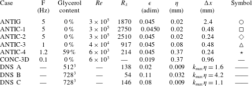
Parameters describing the main datasets used in this paper. ANTI (respectively CON) means impeller rotation in the scooping (respectively unscooping) direction, while G or C refers to the location of the measurement (G for global, C for centre, see figure 1;
 $F$
is the rotation frequency of the impellers in Hz;
 $Re$
is the Reynolds number based on the radius of the tank;
 $Re_{\unicode[STIX]{x1D706}}$
is the Taylor-microscale Reynolds number;
 $\unicode[STIX]{x1D716}$
is the global dimensionless energy dissipation;
 $\unicode[STIX]{x1D702}$
is the Kolmogorov dissipation length scale; and
 $\unicode[STIX]{x0394}x$
represents the spatial resolution in the measurements and the DNS. The last column shows the symbols used to represent the experimental datasets. The experiment CONC-3D corresponds to a case where the velocity is measured by tomographic particle image velocimetry, providing access to the 3 components of velocity.

The numerical data will be based on DNS of INSE at moderate space resolution, so as to be able to accumulate time statistics. They are described in Debue et al. (Reference Debue, Shukla, Kuzzay, Faranda, Saw, Daviaud and Dubrulle2018). The experimental data sets are based on torques and velocity fields measured in the von Kármán flow, using torquemeters and stereoscopic particle image velocimetry at different resolutions and Reynolds numbers. These data are described in Ravelet, Chiffaudel & Daviaud (Reference Ravelet, Chiffaudel and Daviaud2008), Saint-Michel et al. (Reference Saint-Michel, Herbert, Salort, Baudet, Bon Mardion, Bonnay, Bourgoin, Castaing, Chevillard and Daviaud2014). The main characteristics of these data are summarized in table 1. The geometry of the von Kármán flow is depicted in figure 1. The numerical data are by construction noise free and representative of homogeneous isotropic turbulence, but are limited in Reynolds number, and space and time statistics. The experimental data are subject to unavoidable noise and include anisotropy and inhomogeneities, but cover a wide range of scales and Reynolds numbers, with good statistics. In this article, I will mainly use the experimental data, but resort to numerical data to remove any doubt regarding the universality or validity of a given result.
For the sake of clarity, I kept the calculations in the present paper to a minimal complexity level. I refer the reader to the lecture notes of Eyink (Reference Eyink2007--2008), where many details about Onsager’s conjecture, multi-fractal theory and weak solutions can be found.
The von Kármán flow geometry. (a) General view of the experiment in Saclay. The von Kármán flow is generated in a Plexiglas cylinder of radius
 $R$
, filled with fluid at a controlled temperature. The flow is driven by two counter-rotating curve-bladed impellers at frequencies
 $f_{1}=f_{2}$
, rotating with their blades concave face pushing forward, corresponding to the ‘–’ sign in (c) (hereafter referred to as ANTI). For a given
 $F=(f_{1}+f_{2})/2$
, this forcing produces the most intense turbulence, with strongest fluctuations. (b) Schematic design of the experiment. The torque and frequency of each impeller is measured using a torquemeter. Unless explicitly specified, all experimental quantities presented in the present paper are made dimensionless using
 $R$
as a unit of length, and
 $1/(2\unicode[STIX]{x03C0}F)$
as a unit of time. The mean velocity field measured through stereoscopic particle image velocimetry (SPIV) is shown as an inset. The arrows trace the in-plane velocity. The colour traces the out-of-plane velocity. Three types of measurement were done. Either over the whole plane in between the impeller, corresponding to the area covered by the inset (referred to as G for global); or inside the black square (referred as C for centre); or inside the red square (referred to as W for wall). Most of the measurements used in the present essay are done with impellers rotating in the
 $-$
direction and performed in C where the turbulence is the most isotropic and homogeneous. In some cases, we have also added measurements with
 $+$
direction (called CON), and in the W area, to explore the effects of inhomogeneity, anisotropy or forcing. Adapted from Debue (Reference Debue2019).

2 Energetics of turbulence and the cascade picture
2.1 Global energy budget
In 1845, James Prescott Joule published an account of his experiment showing that the application of a 772.24 foot pound force (
 ${\approx}1050$
J) on a paddle stirring a pound of water raises the temperature of the fluid by one degree Fahrenheit. This is an illustration of a global process occurring in most fluids, by which mechanical energy (work) is converted into thermal energy (heat), in agreement with the first law of thermodynamics governing the variation of the fluid total energy in a closed system
 $\unicode[STIX]{x0394}E^{tot}=Q+W$
, as a function of the heat
 $Q$
and work
 $W$
added. The actual fluid energy balance of Joule’s experiment is easily derived from the constitutive equation of the fluid. Taking the scalar product of (1.1) with
 $\boldsymbol{u}$
and integrating over the whole volume, we then get the equation governing the time variation of the total kinetic energy
 $E=(1/2)\unicode[STIX]{x2202}_{t}\int \unicode[STIX]{x1D70C}\boldsymbol{u}^{2}\,\text{d}\,\boldsymbol{x}$
 $$\begin{eqnarray}\displaystyle \unicode[STIX]{x2202}_{t}E & = & \displaystyle \int \unicode[STIX]{x1D70C}\boldsymbol{u}\boldsymbol{\cdot }\boldsymbol{f}\,\text{d}\,\boldsymbol{x}-\unicode[STIX]{x1D708}\int \unicode[STIX]{x1D70C}\left(\unicode[STIX]{x1D735}\boldsymbol{u}\right)^{2}\,\text{d}\,\boldsymbol{x}\end{eqnarray}$$
 $$\begin{eqnarray}\displaystyle & \equiv & \displaystyle P_{inj}-P_{diss},\end{eqnarray}$$
where
 $P_{inj}$
is the injected power through the mechanical work of the paddle, and
 $P_{diss}$
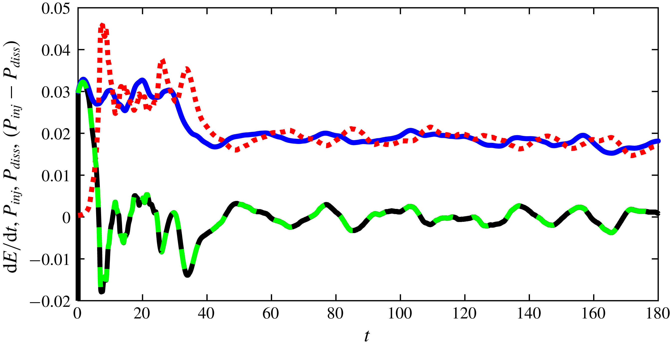
is the dissipated energy through the action of the viscous forces. An example of such balance computed in the statistically stationary DNS A of table 1 is shown in figure 2. Besides checking the validity of (2.2), this figure illustrates a puzzling feature: the injected power and the dissipated power display similar oscillations around a common mean value
 $\overline{P_{inj}}=\overline{P_{diss}}$
, albeit shifted by a constant time lag
 $\unicode[STIX]{x1D70F}_{c}$
. This means that the conversion of work into heat is not instantaneous nor direct, and takes place within the flow via a process that connects different parts of the fluids. To unravel such a process, it is necessary to analyse velocity correlations inside the fluids.
Global energy budget for DNS A. The different terms of (2.2) are plotted as a function of (non-dimensional) time:
 $P_{inj}$
: blue continuous line;
 $P_{diss}$
: red dotted line;
 $\unicode[STIX]{x2202}_{t}E$
: black dotted line. The green dotted line is
 $P_{inj}-P_{diss}$
, which should coincide with
 $\unicode[STIX]{x2202}_{t}E$
in a stationary state. This is indeed the case for this DNS where both curves superpose exactly.

2.2 Velocity correlations and energy spectra
A classical statistical measure of spatial velocity correlations is the function
 $C(\boldsymbol{x},\boldsymbol{r},t)=\langle \boldsymbol{u}(\boldsymbol{x},t)\boldsymbol{u}(\boldsymbol{x}+\boldsymbol{r},t)\rangle$
, where
 $\langle \cdot \rangle$
means statistical average. For any practical application throughout this paper, we shall take advantage, whenever appropriate, of statistical homogeneity, stationarity or isotropy to estimate it through spatial average (
 $\langle A\rangle _{x}\equiv \langle A\rangle$
), time average (
 $\langle A\rangle _{t}\equiv \overline{A}$
) or an angle average over the scale direction (
 $\langle A\rangle _{\unicode[STIX]{x1D719}}$
).
If the turbulence is statistically homogeneous and stationary,
 $C(\boldsymbol{x},\boldsymbol{r},t)$
depends neither on space
 $\boldsymbol{x}$
nor on time
 $t$
, and can be studied through its Fourier transform,
 ${\mathcal{E}}(\boldsymbol{k})=\int \text{e}^{\text{i}\boldsymbol{k}\boldsymbol{\cdot }\boldsymbol{r}}\,\text{d}\boldsymbol{r}$
. If, further, the turbulence is isotropic,
 ${\mathcal{E}}(\boldsymbol{k})$
only depends on
 $k=\Vert \boldsymbol{k}\Vert$
and defines the energy spectrum
 $E(k)=Ak^{d-1}{\mathcal{E}}(k)$
, where
 $A$
is a normalization factor so that
 $\int E(k)\,\text{d}k=0.5\langle \boldsymbol{u}(\boldsymbol{x},t)\boldsymbol{u}(\boldsymbol{x},t)\rangle$
.
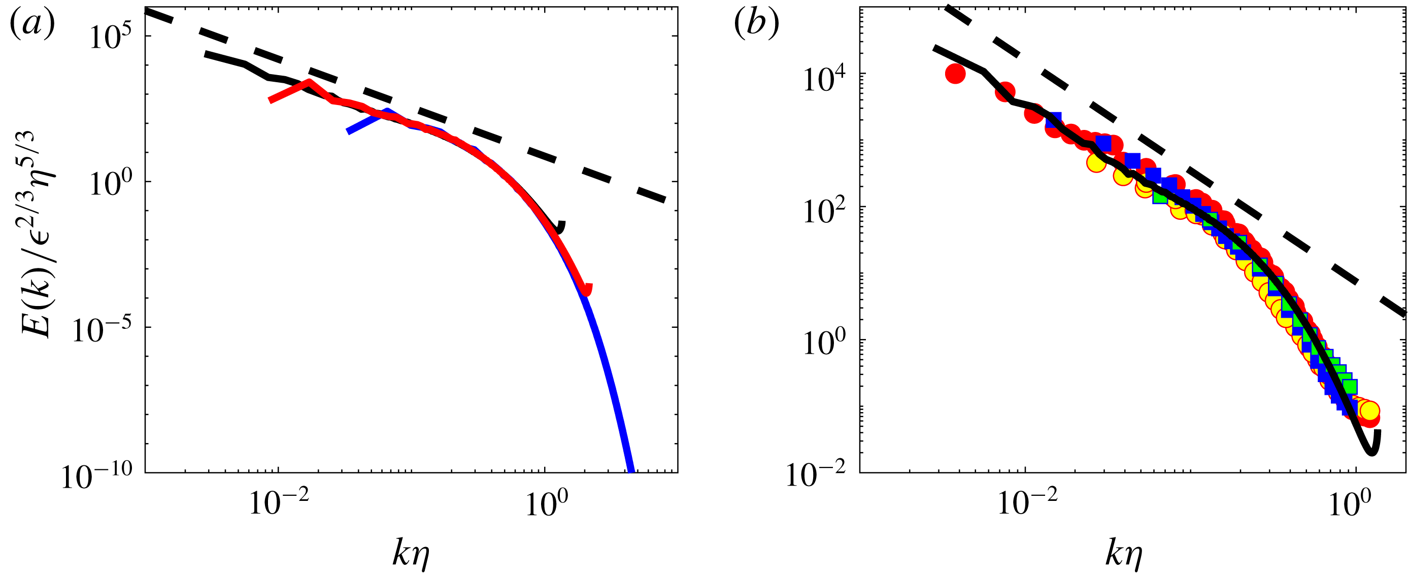
The energy spectrum corresponding to DNS A is shown in figure 3(a). It is self-similar at small wavenumbers (large scales), with a power law approximately equal to
 $k^{-5/3}$
and exponentially decays at large wavenumbers (small scales). The spectrum peaks at a wavenumber
 $k_{f}=1/L_{f}$
corresponding to the forcing scale
 $L_{f}$
. The exponential decay starts around
 $\unicode[STIX]{x1D702}=(\unicode[STIX]{x1D708}^{3}/\unicode[STIX]{x1D716})^{1/4}$
. This is actually the only characteristic scale one can build using the fluid viscosity
 $\unicode[STIX]{x1D708}$
and the mean injected power per unit mass
 $\unicode[STIX]{x1D716}=\overline{P_{inj}}/\unicode[STIX]{x1D70C}{\mathcal{V}}$
where
 ${\mathcal{V}}$
is the volume enclosing the fluid. If we assume that the shape of the spectrum only depends on two variables,
 $\unicode[STIX]{x1D716}$
and
 $\unicode[STIX]{x1D708}$
, we can further build an energy by unit wavenumber
 $\unicode[STIX]{x1D716}^{2/3}\unicode[STIX]{x1D702}^{5/3}$
, so that the energy spectrum is characterized by the function
 $E(k)/\unicode[STIX]{x1D716}^{2/3}\unicode[STIX]{x1D702}^{5/3}$
as a function of
 $k\unicode[STIX]{x1D702}$
, which are the ‘universal coordinates’ considered in figure 3(a). Is this indeed a ‘universal representation’, i.e. does it change when we vary the parameters of the flow?
Spatial kinetic energy spectra at various
 $R_{\unicode[STIX]{x1D706}}$
, and for different forcing or anisotropy conditions. The black dotted line is
 $k^{-5/3}$
. (a) In numerical simulations: DNS B: blue line; DNS C: red line; the black continuous line is from the John Hopkins University Turbulent database (http://turbulence.pha.jhu.edu), at
 $R_{\unicode[STIX]{x1D706}}=433$
(Li et al.
Reference Li, Perlman, Wan, Yang, Burns, Meneveau, Burns, Chen, Szalay and Eyink2008). Picture courtesy F. Nguyen and J-Ph. Laval. (b) In experiments: CON C: red circle, CON W: yellow circle; ANTI C: blue square; ANTI W: green square. Adapted from Debue (Reference Debue2019).

2.3 Universality of the spectrum
The first thing we can change is the Reynolds number. In figure 3(a), we add the energy spectrum of two additional DNSs, one at lower and one at higher Reynolds number. We observe that the range over which the self-similar range is observed is decreased when the Reynolds is decreased, but apart from that, no noticeable change is observed, and the three spectra collapse in universal coordinates. Increasing further the Reynolds number is difficult through numerical simulations. We can turn to experiment to reach larger Reynolds numbers, but then the isotropy and homogeneity conditions will not be met anymore, at least not as cleanly as in numerical simulations. This is anyway a good test of robustness of the universality spectrum.
To illustrate this, we plot in figure 3(b) the spatial energy spectrum, computed for a series of experimental data fields measured by SPIV in a turbulent von Kármán flow, at different spatial locations, using a variety of forcing and flow parameters. The von Kármán flow being globally non-homogeneous, we cannot expect the statistics of the turbulence to be identical everywhere in the tank (Debue et al. Reference Debue, Shukla, Kuzzay, Faranda, Saw, Daviaud and Dubrulle2018). We have selected two special locations in that respect (see figure 1): (i) an area centred around the centre of the experimental set-up, where the mean velocity is zero, and where large velocity fluctuations exist, due to the presence of a strong mixing shear layer; (ii) an area centred around the mid-plane, but located near one of the edges of the tank. At such location, turbulence is highly anisotropic, and dominated by boundary layer effects. Measurements corresponding to these different locations have been associated with different colours in figure 3(b). We see no systematic differences with respect to the numerical energy spectrum.
The flow forcing conditions and the flows properties have also been changed by changing the rotation direction of the impellers (labelled by different symbols in figure 3
b), as well as the flow viscosity. This results in different values of
 $\unicode[STIX]{x1D716}$
(measured independently by torquemeters),
 $R_{\unicode[STIX]{x1D706}}$
(computed using the root-mean-square of the velocity and the viscosity) and
 $\unicode[STIX]{x1D702}$
(computed from the value of the viscosity and
 $\unicode[STIX]{x1D716}$
) for different data sets. Again, we observe that all spectra collapse on the same universal curve as the DNS. This means that properties of the function
 $E(k\unicode[STIX]{x1D702})/\unicode[STIX]{x1D716}^{2/3}\unicode[STIX]{x1D702}^{5/3}$
are very robust, an indication that it is built in the properties of the equations of motions. It was indeed Kolmogorov’s remarkable achievement to derive a simple explanation for the shape of
 $E(k)$
from simple manipulations of the INSE, resulting in what is commonly called the ‘Kolmogorov 1941 theory of turbulence’ (hereafter K41, (Kolmogorov Reference Kolmogorov1941)).
3 The K41 theory and its consequences
3.1 Summary of K41 theory
The explanation of Kolmogorov is based on the Kármán–Howarth–Monin equation (hereafter KHM), an equation that is derived from the Navier–Stokes equations by taking their second moment and assuming local homogeneity (see e.g. Frisch (Reference Frisch1996) for an elementary derivation). The result is a dynamic equation for the correlation function
 $$\begin{eqnarray}\displaystyle \frac{1}{2}\unicode[STIX]{x2202}_{t}C(\boldsymbol{r},t)-{\mathcal{P}}_{\ell } & = & \displaystyle \frac{1}{4}\unicode[STIX]{x1D735}_{\boldsymbol{r}}\boldsymbol{\cdot }\langle \unicode[STIX]{x1D6FF}\boldsymbol{u}(\unicode[STIX]{x1D6FF}\boldsymbol{u})^{2}\rangle -\frac{\unicode[STIX]{x1D708}}{2}\unicode[STIX]{x1D6FB}_{\boldsymbol{r}}^{2}\langle (\unicode[STIX]{x1D6FF}\boldsymbol{u})^{2}\rangle \equiv \unicode[STIX]{x1D735}_{r}\boldsymbol{J}_{\ell }\nonumber\\ \displaystyle & \equiv & \displaystyle -\unicode[STIX]{x1D6F1}_{\ell }^{I}-\unicode[STIX]{x1D6F1}_{\ell }^{\unicode[STIX]{x1D708}},\end{eqnarray}$$
where
 $\langle \rangle$
denotes the statistical average,
 $\unicode[STIX]{x1D735}_{r}$
is the divergence with respect to
 $r$
,
 $\ell =\Vert \boldsymbol{r}\Vert$
denotes the scale,
 ${\mathcal{P}}_{\ell }=\langle \boldsymbol{u}(x)\boldsymbol{\cdot }(\boldsymbol{f}(\boldsymbol{x}+\boldsymbol{r})+\boldsymbol{f}(\boldsymbol{x}-\boldsymbol{r}))\rangle /2$
is a measure of the mean energy injection rate at scale
 $\ell$
,
 $\unicode[STIX]{x1D6FF}\boldsymbol{u}=\boldsymbol{u}(\boldsymbol{x}+\boldsymbol{r})-\boldsymbol{u}(\boldsymbol{x})$
is the velocity increments over a displacement
 $\boldsymbol{r}$
.
For very large value of
 $\ell$
,
 $\overline{{\mathcal{P}}_{\ell }}\rightarrow 0$
since the force and the velocity become uncorrelated. For
 $\ell \rightarrow 0$
,
 $\overline{{\mathcal{P}}_{\ell }}$
tends to
 $\unicode[STIX]{x1D716}$
, the mean energy injection rate (which is also the mean energy dissipation rate). More precisely, for
 $\ell \ll L_{f}$
, where
 $L_{f}$
is the forcing scale, one can Taylor expand
 $\boldsymbol{f}(\boldsymbol{x}+\boldsymbol{r})$
and
 $\boldsymbol{f}(\boldsymbol{x}-\boldsymbol{r})$
to second order in
 $\ell$
to get
 $\overline{{\mathcal{P}}_{\ell }}=\unicode[STIX]{x1D716}+(O(\ell /L_{f})^{2})$
. Now, we note that the last term of the right-hand side of (3.1) is proportional to the viscosity. Kolmogorov first assumes that there is a range of scales
 $L_{min}\ll \ell \ll L_{f}$
– the ‘inertial range’, to be characterized consistently later by providing expression of
 $L_{min}$
– where this term is negligible with respect to the first term of the right-hand side. Looking for a statistically stationary solution, he then takes the time average to get
 $\unicode[STIX]{x1D735}_{\boldsymbol{r}}\overline{\boldsymbol{\cdot }\langle \unicode[STIX]{x1D6FF}\boldsymbol{u}(\unicode[STIX]{x1D6FF}\boldsymbol{u})^{2}\rangle }=-4\unicode[STIX]{x1D716}$
, which can be readily integrated into
 $$\begin{eqnarray}\overline{\langle (\unicode[STIX]{x1D6FF}\boldsymbol{u})^{3}\rangle }=-4\unicode[STIX]{x1D716}\boldsymbol{r}/3.\end{eqnarray}$$
This is called the ‘Kolmogorov
 $4/3$
law’ and is a basic law of turbulence. Kolmogorov further assumes that, over the range of scales where this holds, the function
 ${\mathcal{S}}=\overline{\langle (\unicode[STIX]{x1D6FF}\boldsymbol{u})^{3}\rangle }/\overline{\langle (\unicode[STIX]{x1D6FF}\boldsymbol{u})^{2}\rangle }^{3/2}$
is constant. We shall come back to this assumption later. It means anyway that
 $\overline{\langle (\unicode[STIX]{x1D6FF}\boldsymbol{u})^{2}\rangle }\propto (\unicode[STIX]{x1D716}\ell )^{2/3}$
, with
 $\ell =\Vert \boldsymbol{r}\Vert$
, or, after twice differentiating
 $\unicode[STIX]{x1D6FB}_{\boldsymbol{r}}^{2}\overline{C(\boldsymbol{r})}\propto \unicode[STIX]{x1D716}^{2/3}\ell ^{-4/3}$
, since
 $\overline{\langle (\unicode[STIX]{x1D6FF}\boldsymbol{u})^{2}\rangle }=2\overline{(\langle \boldsymbol{u}^{2}\rangle -C(\boldsymbol{r}))}$
. By Fourier transform, we then get
 $k^{2}E(k)\propto \unicode[STIX]{x1D716}^{2/3}k^{1/3}$
, i.e.
 $E(k)/\unicode[STIX]{x1D716}^{2/3}\unicode[STIX]{x1D702}^{5/3}\propto (k\unicode[STIX]{x1D702})^{-5/3}$
, which is the behaviour we observe for small enough
 $k\unicode[STIX]{x1D702}$
in figure 3. Moreover, the scaling of
 $C(\boldsymbol{r})$
provides us with an estimate of the range of the inertial range. It is indeed characterized by scales
 $\ell \sim 1/k$
such that:
 $$\begin{eqnarray}\unicode[STIX]{x1D735}_{\boldsymbol{r}}\boldsymbol{\cdot }\overline{\langle \unicode[STIX]{x1D6FF}\boldsymbol{u}(\unicode[STIX]{x1D6FF}\boldsymbol{u})^{2}\rangle }\sim \unicode[STIX]{x1D716}\gg \unicode[STIX]{x1D708}\unicode[STIX]{x1D6FB}_{\boldsymbol{r}}^{2}\overline{\langle (\unicode[STIX]{x1D6FF}\boldsymbol{u})^{2}\rangle }\sim \unicode[STIX]{x1D708}\unicode[STIX]{x1D716}^{2/3}\ell ^{-4/3},\end{eqnarray}$$
which is valid as long as
 $\ell \gg (\unicode[STIX]{x1D708}^{3}/\unicode[STIX]{x1D716})^{1/4}=\unicode[STIX]{x1D702}$
, i.e.
 $k\unicode[STIX]{x1D702}\gg 1$
. This is indeed what is observed in figure 3.
3.2 K41 as a phenomenology of cascade and energy balance in scale space
The theory of Kolmogorov successfully explains, as we have seen, the shape of the energy spectrum in universal coordinates in the inertial range. From a broader point of view, it can in fact be seen as a theory of energy balance in the scale-time domain, that helps to build a phenomenology of the energy cascade from the injection scale to the dissipation scales. Indeed, comparing (3.1) with (2.2), we see that KHM describes a global energy balance for
 $C(\boldsymbol{r},t)$
that can be seen as representative of the energy contained at scale
 $\ell =\Vert \boldsymbol{r}\Vert$
. Its time variation is governed by two types of terms: the first one is the divergence, in the scale space, of a vector
 $\boldsymbol{J}_{\ell }=(1/4)\cdot \langle \unicode[STIX]{x1D6FF}\boldsymbol{u}(\unicode[STIX]{x1D6FF}\boldsymbol{u})^{2}\rangle -\unicode[STIX]{x1D708}\unicode[STIX]{x1D735}_{\boldsymbol{r}}\langle (\unicode[STIX]{x1D6FF}\boldsymbol{u})^{2}\rangle /2$
. The second term is independent of scale and describes the energy injection/dissipation
 $\unicode[STIX]{x1D716}$
. The vector
 $\boldsymbol{J}_{\ell }$
can be split into two components, one ‘inertial’
 $\boldsymbol{J}_{\ell }^{I}=(1/4)\langle \unicode[STIX]{x1D6FF}\boldsymbol{u}(\unicode[STIX]{x1D6FF}\boldsymbol{u})^{2}\rangle$
, that only depends on velocity, and a viscous component
 $\boldsymbol{J}_{\ell }^{\unicode[STIX]{x1D708}}=-\unicode[STIX]{x1D708}\unicode[STIX]{x1D735}_{\boldsymbol{r}}\langle (\unicode[STIX]{x1D6FF}\boldsymbol{u})^{2}\rangle /2$
. The vector
 $\boldsymbol{J}_{\ell }$
encodes an energy flux through the scale space (rate at which energy is transferred from scales to scales).
The theory of Kolmogorov already provides us with the scaling of the divergence of the time average of the two components in the inertial range
 $$\begin{eqnarray}\displaystyle \left.\begin{array}{@{}c@{}}\displaystyle \overline{\unicode[STIX]{x1D6F1}_{\ell }^{I}}\equiv -\unicode[STIX]{x1D735}_{\boldsymbol{r}}\boldsymbol{\cdot }\overline{\boldsymbol{J}_{\ell }^{I}}\sim \unicode[STIX]{x1D716},\\ \displaystyle \overline{\unicode[STIX]{x1D6F1}_{\ell }^{\unicode[STIX]{x1D708}}}\equiv -\unicode[STIX]{x1D735}_{\boldsymbol{r}}\boldsymbol{\cdot }\overline{\boldsymbol{J}_{\ell }^{\unicode[STIX]{x1D708}}}\sim \unicode[STIX]{x1D708}\unicode[STIX]{x1D716}^{2/3}\ell ^{-4/3}\sim \unicode[STIX]{x1D716}\left(\frac{\ell }{\unicode[STIX]{x1D702}}\right)^{-4/3},\end{array}\right\} & & \displaystyle\end{eqnarray}$$
which is valid as long as
 $\ell \geqslant \unicode[STIX]{x1D702}$
. At
 $\ell \sim \unicode[STIX]{x1D702}$
, the two terms coincide. The typical velocity at this scales is
 $u_{\unicode[STIX]{x1D702}}\sim (\unicode[STIX]{x1D702}\overline{\boldsymbol{J}_{\ell }^{I}})^{1/3}\sim (\unicode[STIX]{x1D716}\unicode[STIX]{x1D702})^{1/3}$
, so that the Reynolds number at this scale is
 $Re(\unicode[STIX]{x1D702})=(\unicode[STIX]{x1D716}\unicode[STIX]{x1D702}^{4})^{1/3}/\unicode[STIX]{x1D708}=1$
: viscosity becomes the preponderant process and the flow is laminar below
 $\unicode[STIX]{x1D702}$
. It is then meaningful to perform a Taylor expansion on the velocity, to get the scaling of the velocity increment as
 $\unicode[STIX]{x1D6FF}u\sim \boldsymbol{r}\boldsymbol{\cdot }\unicode[STIX]{x1D735}\boldsymbol{u}=O(\ell \sqrt{\unicode[STIX]{x1D716}/\unicode[STIX]{x1D708}})$
, where we have used
 $\unicode[STIX]{x1D716}\sim \unicode[STIX]{x1D708}(\unicode[STIX]{x1D6FB}\boldsymbol{u})^{2}$
. We thus infer the following scaling laws for scales below
 $\unicode[STIX]{x1D702}$
as
 $$\begin{eqnarray}\displaystyle \left.\begin{array}{@{}c@{}}\displaystyle \overline{\unicode[STIX]{x1D6F1}_{\ell }^{I}}\sim \left(\frac{\unicode[STIX]{x1D716}}{\unicode[STIX]{x1D708}}\right)^{3/2}\ell ^{2}\sim \unicode[STIX]{x1D716}\left(\frac{\ell }{\unicode[STIX]{x1D702}}\right)^{2},\\ \displaystyle \overline{\unicode[STIX]{x1D6F1}_{\ell }^{\unicode[STIX]{x1D708}}}\sim \unicode[STIX]{x1D708}\frac{\unicode[STIX]{x1D716}}{\unicode[STIX]{x1D708}}\sim \unicode[STIX]{x1D716}.\end{array}\right\} & & \displaystyle\end{eqnarray}$$
The viscous component then carries most of the flux, and the inertial component vanishes like
 $\ell ^{2}$
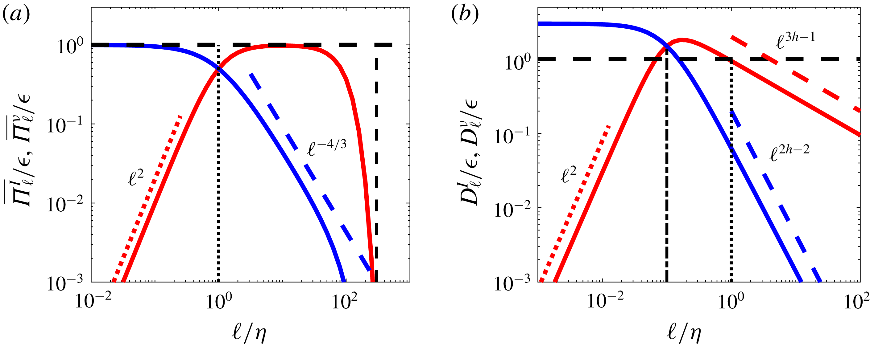
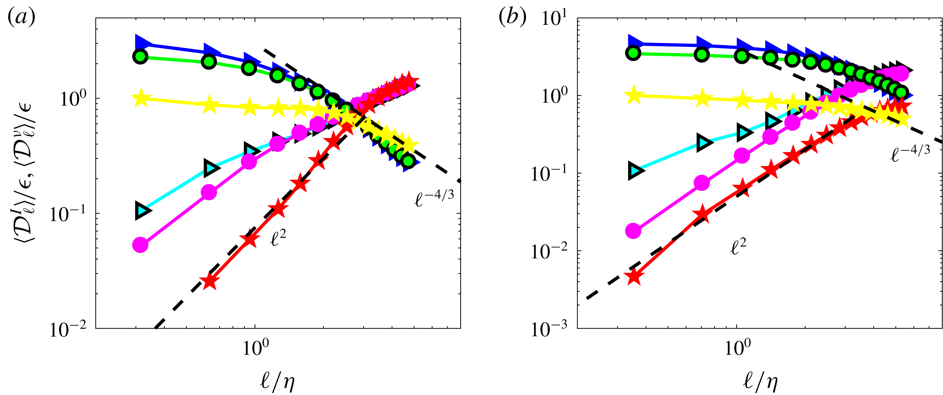
. The different scaling laws are summarized in figure 4(a). The overall picture associated with these scalings is that of an ‘energy cascade’: the energy is injected at large scale at a rate
 $\unicode[STIX]{x1D716}$
. It is transferred down the scales at a constant rate
 $\unicode[STIX]{x1D716}$
by the inertial flux, until it reaches the scale
 $\unicode[STIX]{x1D702}$
where the viscous flux takes over, and carries this flux down to
 $\ell \sim 0$
(actually the hydrodynamic scale) where it is transformed into heat. The time lag
 $\unicode[STIX]{x1D70F}_{c}$
observed in figure 2 between the time of energy injection and energy dissipation corresponds then to a ‘cascade time’, the time it takes for a parcel of energy to be transferred from scale
 $L_{f}$
to
 $\unicode[STIX]{x1D702}$
.
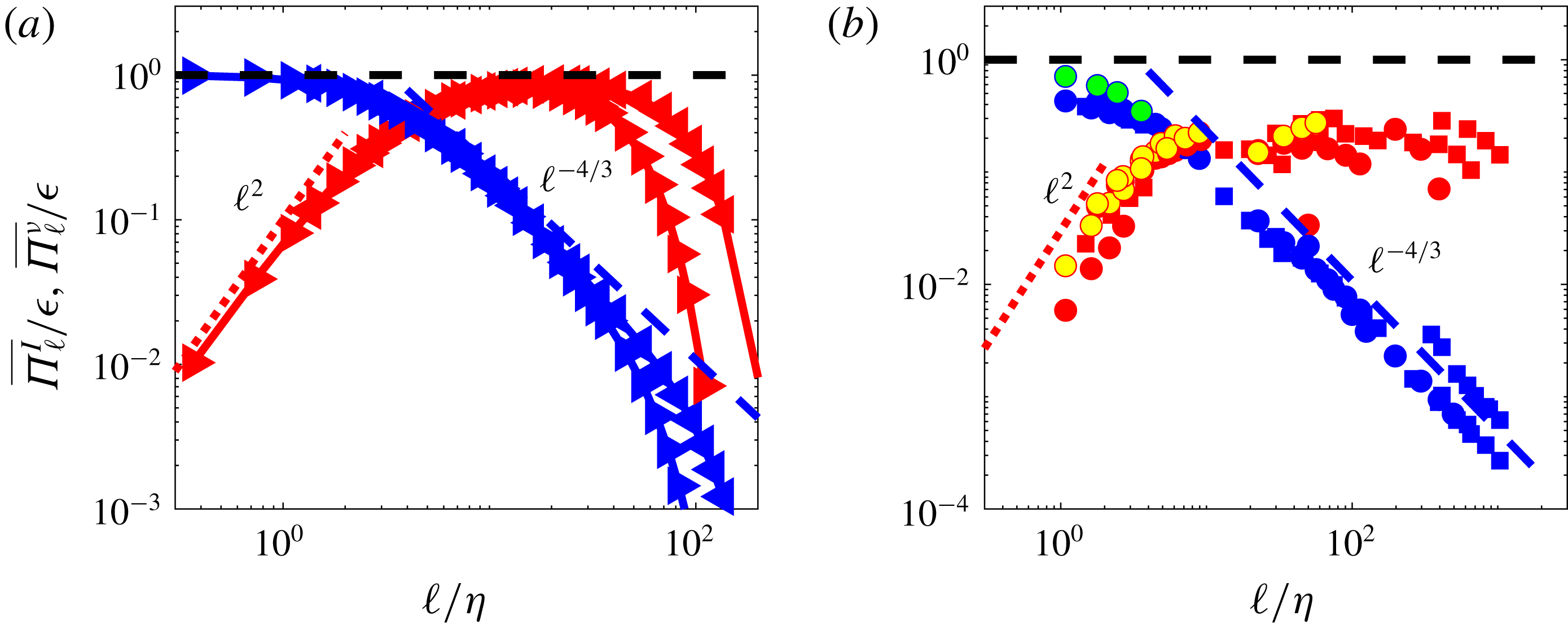
The validity of this picture can be tested against DNS of homogeneous, isotropic turbulence. This is done in figure 5(a). One sees that all the scalings laws of the K41 picture of turbulence are satisfied. Moreover, the ‘inertial’ range indeed expands as
 $L_{f}/\unicode[STIX]{x1D702}$
.
K41 versus multi-fractal picture of turbulence. (a) K41 picture: the energy injected at scale
 $L_{f}$
(vertical black dashed line) is transferred at a constant rate
 $\unicode[STIX]{x1D716}$
by the energy flux
 $\overline{\unicode[STIX]{x1D6F1}_{\ell }^{I}}$
(red line) down the scale where it becomes equal to the viscous flux
 $\overline{\unicode[STIX]{x1D6F1}_{\ell }^{\unicode[STIX]{x1D708}}}$
(blue line). From downwards on, it is transported by the latter to the smallest hydrodynamic scale, where it is dissipated into heat. In the inertial range, the energy flux is constant, and the viscous flux increases like
 $\ell ^{-4/3}$
. In the dissipative range, the viscous flux is constant, while the energy flux decreases like
 $\ell ^{2}$
in the dissipative range. The energy flux and the viscous flux become equal at the Kolmogorov scale, indicated by a black dotted line. (b) Multi-fractal picture: the energy is transferred at smaller scale by the energy flux (red line) up to the scale
 $\unicode[STIX]{x1D702}_{h}$
(vertical dashed dotted line) where the energy flux and the viscous flux (blue line) balance. In the inertial range, the energy flux and viscous flux scale respectively like
 $\ell ^{3h-1}$
and
 $\ell ^{2h-2}$
, while they obey the same scaling than in the K41 picture in the dissipative range. When
 $h<1/3$
, the energy flux and the viscous flux become equal at a scale smaller than the Kolmogorov scale, indicated by a black dotted line.

Test of K41 picture. (a) in numerical simulations: left-pointing triangles: DNS B; right-pointing triangles: DNS A. Red symbols: mean energy flux
 $\overline{\unicode[STIX]{x1D6F1}_{\ell }^{I}}/\unicode[STIX]{x1D716}$
; blue symbol: mean viscous flux
 $\overline{\unicode[STIX]{x1D6F1}_{\ell }^{\unicode[STIX]{x1D708}}}/\unicode[STIX]{x1D716}$
. The red dotted line is
 $0.1(\ell /\unicode[STIX]{x1D702})^{2}$
and the blue dashed line is
 $5(\ell /\unicode[STIX]{x1D702})^{-4/3}$
. (b) In experiments using SPIV data: mean energy flux for CON C: red circle, CON W: yellow circle; ANTI C: red square, ANTI C: yellow square; mean viscous flux for CON C: blue circle, CON W: green circle, ANTI C: blue square, ANTI W: green square. Adapted from Debue (Reference Debue2019).

3.3 Universality of the energy budget in scale
The energy budget in the scale given by (3.1) and its associated picture of the energy cascade (figure 4
a,b), derived for ideal, homogeneous turbulence, is actually very robust. Not surprisingly (remember the results for the spectra), the scaling properties of the divergence of the time average of the two components of the energy flux density
 $\boldsymbol{J}_{\ell }$
, reported in figure 5(b), display a remarkable agreement with the expected scaling laws, with no systematic effect due to different locations (coded by colour), or forcing condition (coded by symbols). The main difference with the results of the DNS is the value of the plateau for
 $\overline{\unicode[STIX]{x1D6F1}_{\ell }^{I}}$
, which is around
 $0.3$
rather than
 $1$
. This is because, due to the planar measurement, we can only have access to the in-plane component of this flux. If the flow were isotropic, we would thus get
 $2/3$
of the total value. The von Kármán flow is highly anisotropic at this location, so that the out-of-plane component actually carries a large fraction of the flux, which explains our result.
3.4 Statistical properties of the energy cascade in scale space
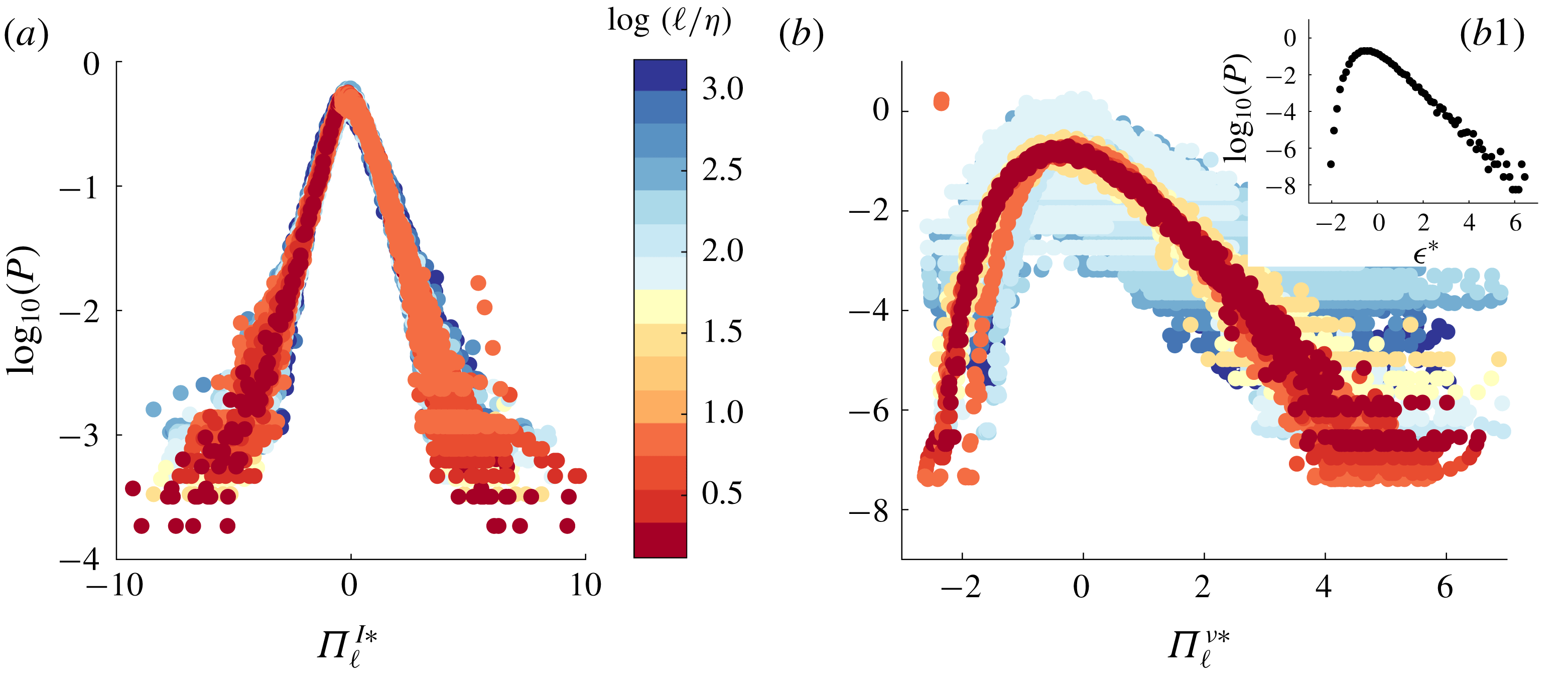
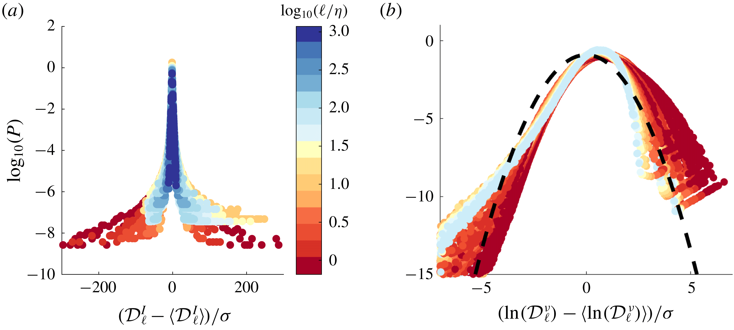
Experiments provide large data sets of independent realizations of the cascade so that we can use them to study the statistical properties of the energy cascade in scale space. In figure 6(a,b), we plot the probability distribution functions (PDFs) of
 $\unicode[STIX]{x1D6F1}_{\ell }^{I}$
and
 $\unicode[STIX]{x1D6F1}_{\ell }^{\unicode[STIX]{x1D708}}$
, obtained through velocity measurements at uncorrelated times at the centre of the experiment, for a flow forced in the scooping direction (minus sign direction in figure 1(c)), for scales ranging in
 $1\leqslant \ell /\unicode[STIX]{x1D702}\leqslant 10^{3}$
. We see that the two PDFs are very different and vary significantly with scale: the PDF of
 $\unicode[STIX]{x1D6F1}_{\ell }^{I}$
is almost symmetrical around
 $0$
with exponential tails widening as the scale increases; the PDFs of
 $\unicode[STIX]{x1D6F1}_{\ell }^{\unicode[STIX]{x1D708}}$
are lognormal (parabolic in log–log plot, not shown) with tails narrowing as the scale increases.
Both PDFs however carry the same universal features: when plotted using centred reduced variables
 $\unicode[STIX]{x1D6F1}_{\ell }^{I\ast }=(\unicode[STIX]{x1D6F1}_{\ell }^{I}-\overline{\unicode[STIX]{x1D6F1}_{\ell }^{I}})/\unicode[STIX]{x1D70E}^{I}$
and
 $\unicode[STIX]{x1D6F1}_{\ell }^{\unicode[STIX]{x1D708}\ast }=(\unicode[STIX]{x1D6F1}_{\ell }^{\unicode[STIX]{x1D708}}-\overline{\unicode[STIX]{x1D6F1}_{\ell }^{\unicode[STIX]{x1D708}}})/\unicode[STIX]{x1D70E}^{\unicode[STIX]{x1D708}}$
, the PDFs collapse on two universal curves, see figure 6(a,b). The PDF of
 $\unicode[STIX]{x1D6F1}_{\ell }^{\unicode[STIX]{x1D708}\ast }$
is similar in shape to the PDF of energy dissipation (displayed in figure 6
b1). Summarizing, we see that both the local energy transfer
 $\unicode[STIX]{x1D6F1}_{\ell }^{I}$
and dissipation
 $\unicode[STIX]{x1D6F1}_{\ell }^{\unicode[STIX]{x1D708}}$
have universal statistical properties, following
 $$\begin{eqnarray}\displaystyle & \displaystyle P(\unicode[STIX]{x1D6F1}_{\ell }^{I})={\mathcal{P}}^{{\mathcal{I}}}\left(\frac{\unicode[STIX]{x1D6F1}_{\ell }^{I}-\overline{\unicode[STIX]{x1D6F1}_{\ell }^{I}}}{\unicode[STIX]{x1D70E}^{I}(\ell )}\right), & \displaystyle\end{eqnarray}$$
 $$\begin{eqnarray}\displaystyle & \displaystyle P(\unicode[STIX]{x1D6F1}_{\ell }^{\unicode[STIX]{x1D708}})={\mathcal{P}}^{\unicode[STIX]{x1D708}}\left(\frac{\unicode[STIX]{x1D6F1}_{\ell }^{\unicode[STIX]{x1D708}}-\overline{\unicode[STIX]{x1D6F1}_{\ell }^{\unicode[STIX]{x1D708}}}}{\unicode[STIX]{x1D70E}^{\unicode[STIX]{x1D708}}(\ell )}\right), & \displaystyle\end{eqnarray}$$
where all the scale dependences are encoded in the means
 $\overline{\unicode[STIX]{x1D6F1}_{\ell }^{I}},\overline{\unicode[STIX]{x1D6F1}_{\ell }^{\unicode[STIX]{x1D708}}}$
and the standard deviations (std)
 $\unicode[STIX]{x1D70E}^{I}(\ell ),\unicode[STIX]{x1D70E}^{\unicode[STIX]{x1D708}}(\ell )$
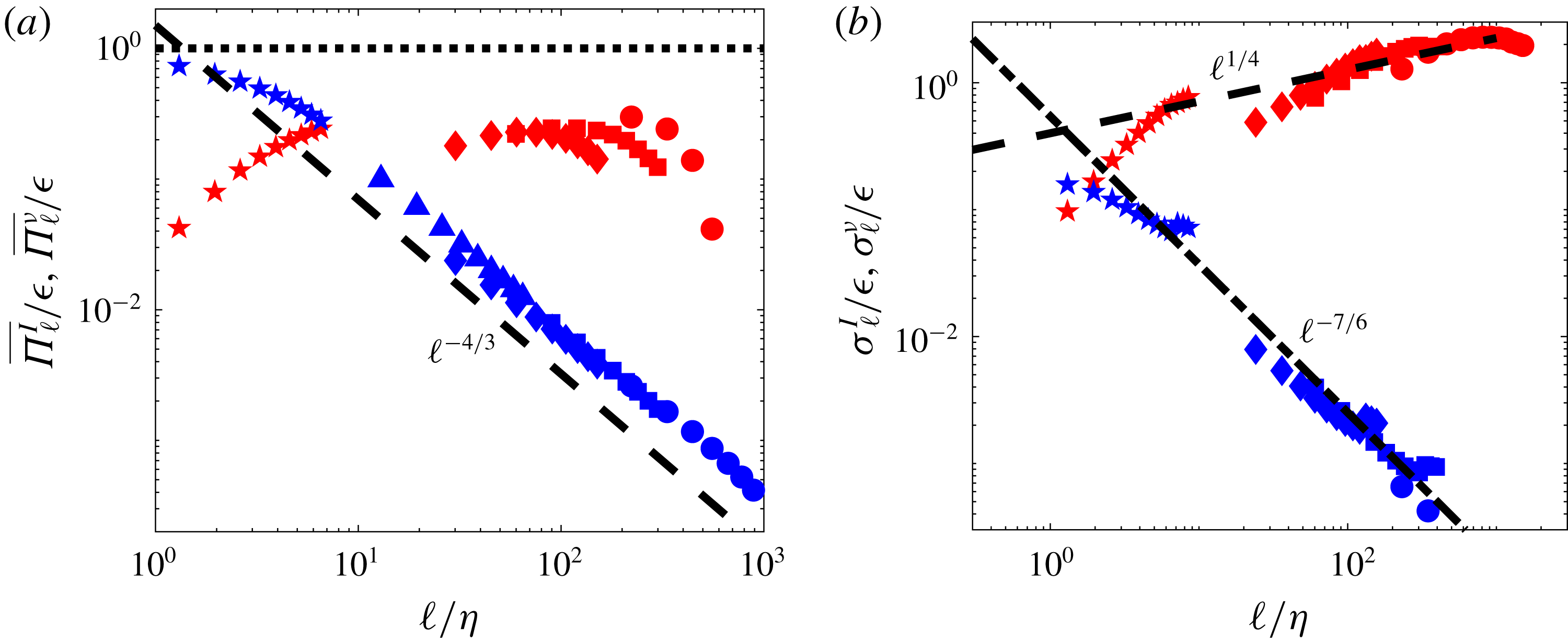
shown in figure 7.
PDFs of flux terms, centred and reduced as explained in the text, for experiments ANTIG and ANTIC-1 to ANTIC-4 (see figure 7 for corresponding mean and standard deviation and table 1 for symbols). (a) Centred and reduced PDF of
 $\unicode[STIX]{x1D6F1}_{\ell }^{I}$
at different scale, coded by colour, following the colour bar. (b) Centred and reduced PDF of
 $\unicode[STIX]{x1D6F1}_{\ell }^{\unicode[STIX]{x1D708}}$
at different scale, coded by colour. Inset (b1): centred and reduced PDF of dissipation.

Scale variation of the mean and standard deviations of the flux terms for experiments ANTIG and ANTIC-1 to ANTIC-4. (a) Time average:
 $\overline{\unicode[STIX]{x1D6F1}_{\ell }^{I}}$
: red symbols;
 $\overline{\unicode[STIX]{x1D6F1}_{\ell }^{\unicode[STIX]{x1D708}}}$
: blue symbols. (b) Standard deviation
 $\unicode[STIX]{x1D70E}_{\ell }^{I}$
: red symbols;
 $\unicode[STIX]{x1D70E}_{\ell }^{\unicode[STIX]{x1D708}}$
: blue symbols. The black dashed line is
 $\ell ^{1/4}$
. The dashed-dot line in (b) is
 $\ell ^{-4/3}\ell ^{1/6}$
deduced from the
 $\ell ^{2}$
scaling of the std ratio shown in figure 8(a) and the scaling of
 $\unicode[STIX]{x1D70E}_{\ell }^{I}$
.

Not surprisingly, the means of
 $\unicode[STIX]{x1D6F1}_{\ell }^{\unicode[STIX]{x1D708}}$
and
 $\unicode[STIX]{x1D6F1}_{\ell }^{I}$
obey the Kolmogorov scaling sketched in figure 4(a). The standard deviations however, display new behaviours that are not predicted by K41 theory: the std of
 $\unicode[STIX]{x1D6F1}_{\ell }^{\unicode[STIX]{x1D708}}$
decreases with increasing scale with an exponent slightly smaller than
 $-4/3$
, while the std of
 $\unicode[STIX]{x1D6F1}_{\ell }^{I}$
increases slightly with scales (like
 $\ell ^{0.25}$
). To understand such behaviour, one needs to leave empirical observation and dig deeper into theoretical consequences and meaning of K41.
4 K41 theory and symmetries: successes and limitations
4.1 Some basic symmetries of Navier–Stokes
As pointed out by Frisch (Reference Frisch1996), K41 theory is deeply connected with basic symmetry properties of the Navier–Stokes equations (1.1), namely:
(i) space translation (homogeneity):
 $\boldsymbol{x}\rightarrow \boldsymbol{x}+\boldsymbol{r}$
, for arbitrary
$\boldsymbol{r}$
;
(ii) time translation (stationarity):
$t\rightarrow t+\unicode[STIX]{x1D70F}$
, for arbitrary
$\unicode[STIX]{x1D70F}$
;(iii) rescaling:
$(t,\boldsymbol{x},\boldsymbol{u})\rightarrow (\unicode[STIX]{x1D706}^{2}t,\unicode[STIX]{x1D706}\boldsymbol{x},\unicode[STIX]{x1D706}^{-1}\boldsymbol{u})$
, for arbitrary
$\unicode[STIX]{x1D706}$
; and in the inviscid limit,
$\unicode[STIX]{x1D708}\rightarrow 0$
:(iv) time reversal:
$(t,\boldsymbol{u})\rightarrow (-t,-\boldsymbol{u})$
,(v)
$h$
rescaling:
$(t,\boldsymbol{x},\boldsymbol{u})\rightarrow (\unicode[STIX]{x1D706}^{1-h}t,\unicode[STIX]{x1D706}\boldsymbol{x},\unicode[STIX]{x1D706}^{h}\boldsymbol{u})$
, for arbitrary
$\unicode[STIX]{x1D706}$
and
$h$
. Note that the rescaling (iii) is equivalent to a
$-1$
rescaling (property (v) with
$h=-1$
).


Let us explore in more details such connections and their consequences.
4.2 Rescaling symmetry breaking and generalized skewness
A basic ingredient of K41 is that the skewness
 ${\mathcal{S}}=\overline{\langle (\unicode[STIX]{x1D6FF}\boldsymbol{u})^{3}\rangle }/\overline{\langle (\unicode[STIX]{x1D6FF}\boldsymbol{u})^{2}\rangle }^{3/2}$
is constant or equivalently, the generalized skewness
 ${\mathcal{S}}_{1}\equiv \overline{\unicode[STIX]{x1D6F1}_{\ell }^{I}}/\overline{(\unicode[STIX]{x1D6F1}_{\ell }^{\unicode[STIX]{x1D708}})}^{3/2}$
scales like
 ${\mathcal{S}}_{1}\sim \ell ^{2}$
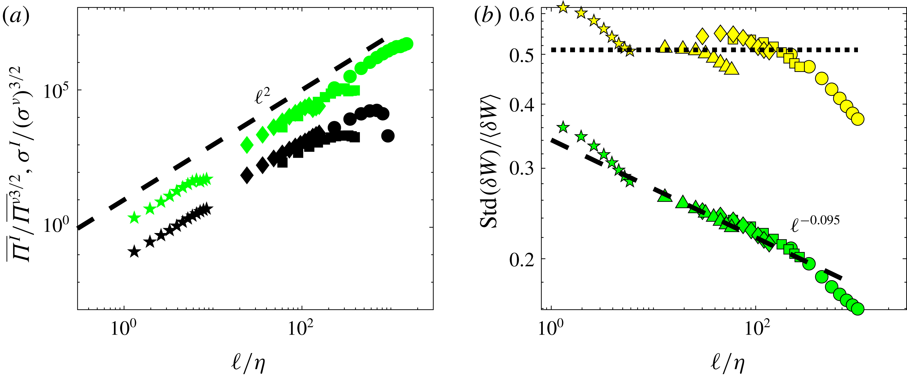
. This is very well satisfied by the experimental data up to at least the Kolmogorov scale, as shown in figure 8(a). Moreover, the scaling law is also satisfied by the standard deviations
 $\unicode[STIX]{x1D70E}_{\ell }^{I}/(\unicode[STIX]{x1D70E}_{\ell }^{\unicode[STIX]{x1D708}})^{3/2}\sim \ell ^{2}$
. Because of the universal properties of the PDFs of
 $\unicode[STIX]{x1D6F1}_{\ell }^{\unicode[STIX]{x1D708}}$
and
 $\unicode[STIX]{x1D6F1}_{\ell }^{I}$
(3.7), this means that any generalized skewness
 ${\mathcal{S}}_{q}\equiv \overline{(\unicode[STIX]{x1D6F1}_{\ell }^{I})^{q}}/\overline{(\unicode[STIX]{x1D6F1}_{\ell }^{\unicode[STIX]{x1D708}})^{q}}^{3/2}$
scales like
 $\ell ^{2q}$
.
Test of rescaling symmetry for experiments ANTIG and ANTIC-1 to ANTIC-4. (a) For the flux
 $\unicode[STIX]{x1D6F1}_{\ell }^{I}$
and
 $\unicode[STIX]{x1D6F1}_{\ell }^{\unicode[STIX]{x1D708}}$
via the generalized skewness
 $\overline{\unicode[STIX]{x1D6F1}_{\ell }^{I}}/\overline{\unicode[STIX]{x1D6F1}_{\ell }^{\unicode[STIX]{x1D708}}}^{3/2}$
(black symbols) and std ratio
 $\unicode[STIX]{x1D70E}_{\ell }^{I}/(\unicode[STIX]{x1D70E}_{\ell }^{\unicode[STIX]{x1D708}})^{3/2}$
(green symbols). The dashed line is
 $\ell ^{2}$
. (b) For the wavelet velocity increments
 $\unicode[STIX]{x1D6FF}W$
at different scales, using ratio of standard deviation to average for
 $\unicode[STIX]{x1D6FF}W$
(green symbols) and
 $\unicode[STIX]{x1D6FF}W^{C}$
(yellow symbols). For self-similar variables, the ratio should be constant (dotted line), which is true for
 $\unicode[STIX]{x1D6FF}W^{C}$
but not for
 $\unicode[STIX]{x1D6FF}W$
. The dashed line is
 $\ell ^{-0.095}$
.

On the other hand, if we apply the
 $h$
rescaling symmetry (iv) to
 $\unicode[STIX]{x1D6F1}_{\ell }^{I}$
and
 $\unicode[STIX]{x1D6F1}_{\ell }^{\unicode[STIX]{x1D708}}$
, we notice that they are respectively rescaled by a factor
 $\unicode[STIX]{x1D706}^{3h-1}$
and
 $\unicode[STIX]{x1D706}^{2h-2}$
, so that all the generalized skewness values
 ${\mathcal{S}}_{q}$
are rescaled by a factor
 $\unicode[STIX]{x1D706}^{2q}$
, in agreement with their observed scaling. The minimal hypothesis to explain the experimental behaviour of the high-order properties of the energy cascade is therefore that it is statistically invariant by
 $h$
rescaling, with no special emphasis on a particular
 $h$
so far.
Furthermore, if one compares the individual behaviours of
 $\unicode[STIX]{x1D6F1}_{\ell }^{I}$
and
 $\unicode[STIX]{x1D6F1}_{\ell }^{\unicode[STIX]{x1D708}}$
under
 $h$
rescaling symmetry (iv) and compare these with the scaling behaviours of the K41 theory, we see that they are compatible with respectively
 $3h-1=0$
and
 $2h-2=-4/3$
, i.e.
 $h=1/3$
for both. This mean that the rescaling symmetry (iii) is broken, so that viscosity becomes irrelevant (in agreement with the ‘inertial range’ assumption) and only
 $h$
rescaling (v) with
 $h=1/3$
should be considered. There is however no understanding at this stage of how the special value
 $h=1/3$
is selected with respect to other possible values. For this, we need to dive more deeply into the energy cascade and its properties.
4.3 Energy cascade and inhomogeneity
Taking into account the K41 scaling, we can take the limit
 $\ell \rightarrow 0$
of the KHM equation (3.1) to get
 $$\begin{eqnarray}{\textstyle \frac{1}{2}}\unicode[STIX]{x2202}_{t}\langle u^{2}(x,t)\rangle -\langle \boldsymbol{f}\boldsymbol{\cdot }\boldsymbol{u}\rangle =-\unicode[STIX]{x1D708}\langle (\unicode[STIX]{x1D6FB}u)^{2}(x,t)\rangle ,\end{eqnarray}$$
which is nothing but the global energy budget equation (2.2). Small-scale behaviour of the energy cascade picture has, therefore, an immediate consequence on the enstrophy scaling. Indeed, in homogeneous turbulence, the enstrophy
 $\langle \unicode[STIX]{x1D714}^{2}(x,t)\rangle =\langle (\unicode[STIX]{x1D6FB}u)^{2}(x,t)\rangle$
, so we get from (4.1)
 $$\begin{eqnarray}\unicode[STIX]{x1D6FA}\equiv \overline{\langle \unicode[STIX]{x1D714}^{2}(x,t)\rangle }=\frac{\unicode[STIX]{x1D716}}{\unicode[STIX]{x1D708}}.\end{eqnarray}$$
For this equality to hold, it means that there is in the flow at least one point where the magnitude of the vorticity
 $\unicode[STIX]{x1D74E}=\unicode[STIX]{x1D735}\times \boldsymbol{u}$
exceeds the threshold:
 $|\unicode[STIX]{x1D714}|\geqslant \sqrt{\unicode[STIX]{x1D716}/\unicode[STIX]{x1D708}}=\unicode[STIX]{x1D716}^{1/3}\unicode[STIX]{x1D702}^{-2/3}$
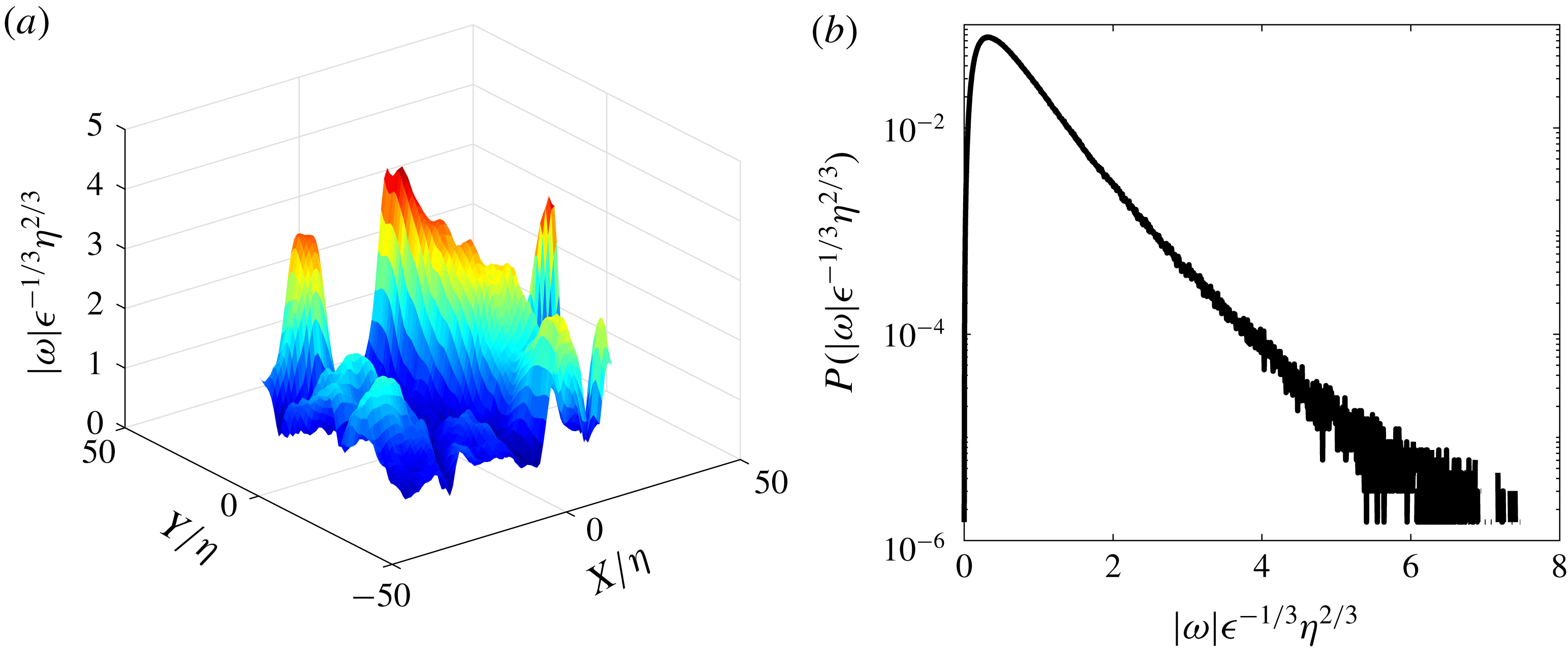
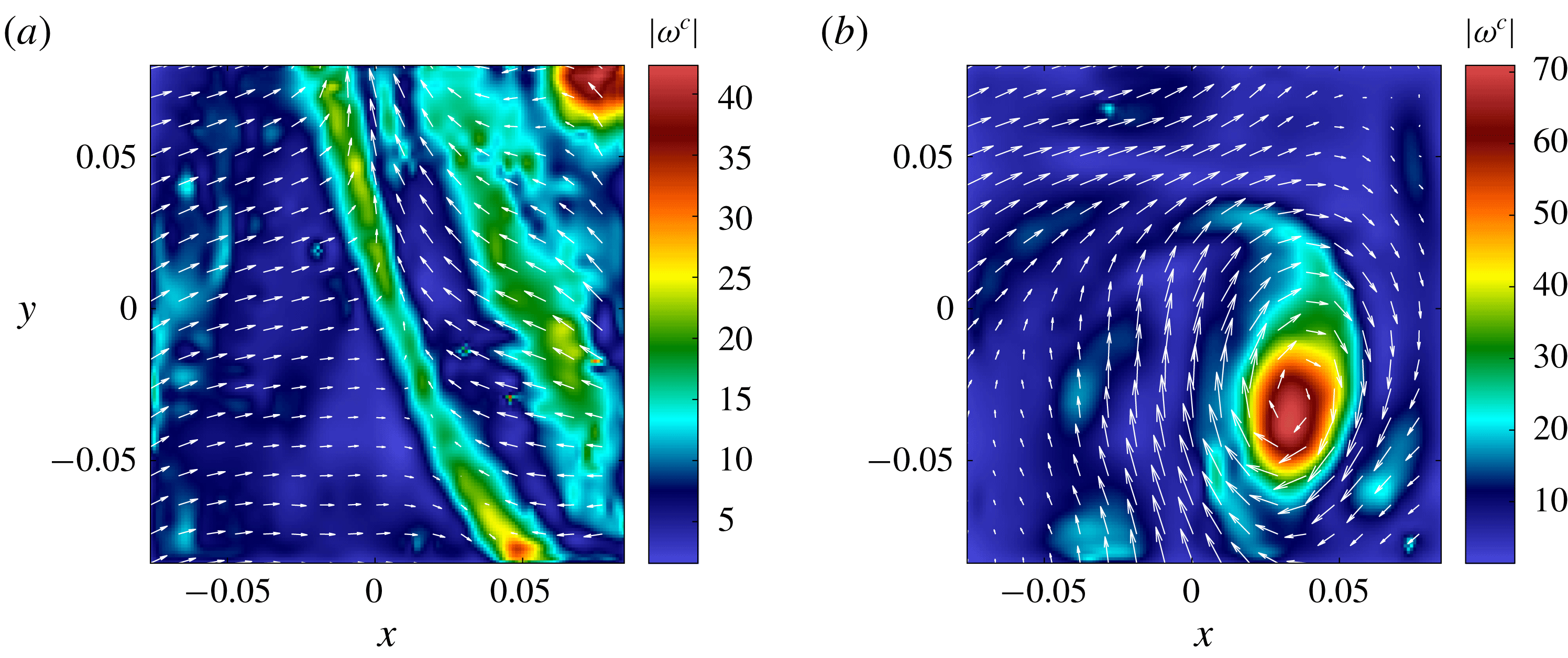
. There are in fact many points where this happens, as can be seen in figure 9(a), where peaks of vorticity, over regions of size
 $30\unicode[STIX]{x1D702}$
, exist. Overall, the vorticity field is very intermittent, meaning that if the homogeneity postulated by Kolmogorov holds, it is only valid in a statistical sense (Frisch Reference Frisch1996).
Non-dimensional vorticity magnitude (a) and PDF of non-dimensional vorticity magnitude (b) in the experiment CONC-3D. The figures are drawn using unpublished data collected by the EXPLOIT collaboration (F. Daviaud, B. Dubrulle, P. Debue, V. Valori, J.-P. Laval, J.-M. Foucaut, Ch. Cuvier, Y. Ostovan), with permission.

4.4 Vortex stretching and
$1/3$
rescaling

Another measure of the intermittency of the vorticity field is provided by the PDF of the magnitude of the vorticity, shown in figure 9(b). It is highly non-Gaussian, with tails extending over values much larger than
 $\unicode[STIX]{x1D716}^{1/3}\unicode[STIX]{x1D702}^{-2/3}$
. Such behaviour requires a mechanism of amplification of vorticity: indeed, the forcing injects a typical value of the velocity
 $(\unicode[STIX]{x1D716}L)^{1/3}$
, resulting in a typical vorticity of
 $\unicode[STIX]{x1D716}^{1/3}L^{-2/3}$
, smaller than the threshold by a value
 $(\unicode[STIX]{x1D702}/L)^{2/3}$
. The mechanism has been identified by Taylor (Reference Taylor1938). It is based on the observation that, in the inviscid limit, both vorticity
 $\unicode[STIX]{x1D714}_{i}$
and lines
 $\ell _{i}$
are dynamically stretched by the velocity field, according to
 $$\begin{eqnarray}\unicode[STIX]{x2202}_{t}A_{i}+u_{j}\unicode[STIX]{x2202}_{j}A_{i}=A_{j}\unicode[STIX]{x2202}_{j}u_{i},\end{eqnarray}$$
where
 $A_{i}=\unicode[STIX]{x1D714}_{i}$
or
 $\ell _{i}$
. In a first approximation, let us ignore viscosity and concentrate on the Lagrangian kinematic of vorticity in the frame where the tensor
 $\unicode[STIX]{x2202}_{j}u_{i}$
is diagonal
 $\unicode[STIX]{x2202}_{j}u_{i}=\text{Diag}(\unicode[STIX]{x1D706}_{1},\unicode[STIX]{x1D706}_{2},\unicode[STIX]{x1D706}_{3})$
, with
 $|\unicode[STIX]{x1D706}_{1}|\geqslant |\unicode[STIX]{x1D706}_{2}|\geqslant |\unicode[STIX]{x1D706}_{3}|$
. Due to incompressibility,
 $\unicode[STIX]{x1D706}_{1}+\unicode[STIX]{x1D706}_{2}+\unicode[STIX]{x1D706}_{3}=0$
, so that either all the
 $\unicode[STIX]{x1D706}_{i}$
are real, and
 $\unicode[STIX]{x1D706}_{1}\unicode[STIX]{x1D706}_{3}\leqslant 0$
, or one is real, equal say to
 $\unicode[STIX]{x1D706}_{1}$
, and the other two are complex conjugates, equal to
 $\unicode[STIX]{x1D706}_{2}=\unicode[STIX]{x1D706}_{3}^{\ast }$
, with
 $\unicode[STIX]{x1D706}_{1}\times \text{real}(\unicode[STIX]{x1D706}_{2})\leqslant 0$
. In such a frame, the kinematic behaviour associated with (4.3) is simply
 $$\begin{eqnarray}D_{t}A_{i}=Diag(\unicode[STIX]{x1D706}_{1}A_{1},\unicode[STIX]{x1D706}_{2}A_{2},\unicode[STIX]{x1D706}_{3}A_{3}).\end{eqnarray}$$
A blob of initial vorticity
 $(\unicode[STIX]{x1D714}_{1},\unicode[STIX]{x1D714}_{2},\unicode[STIX]{x1D714}_{3})$
with characteristic dimension
 $(\unicode[STIX]{x1D6FF}_{1},\unicode[STIX]{x1D6FF}_{2},\unicode[STIX]{x1D6FF}_{3})$
will experience two processes: its magnitude along the direction corresponding to the eigenvalue with largest positive real part (say
 $\unicode[STIX]{x1D706}_{1}$
) will be exponentially amplified
 $\unicode[STIX]{x1D714}_{1}=\exp (\unicode[STIX]{x1D706}_{1}t)$
, while its dimension along the direction corresponding to the eigenvalue with largest negative real part (say
 $\unicode[STIX]{x1D706}_{3}$
) will be exponentially compressed
 $\unicode[STIX]{x1D6FF}_{3}=\exp (-|\unicode[STIX]{x1D706}_{3}|t)$
. During such a process, the maximum vorticity
 $\unicode[STIX]{x1D714}_{max}$
will then scale like
 $$\begin{eqnarray}\unicode[STIX]{x1D714}_{max}=\unicode[STIX]{x1D6FF}_{3}^{h_{\unicode[STIX]{x1D714}}},\end{eqnarray}$$
with
 $h_{\unicode[STIX]{x1D714}}=-\unicode[STIX]{x1D706}_{1}/|\unicode[STIX]{x1D706}_{3}|$
. Direct numerical simulations of this inviscid kinematic stage are difficult, since they require tracking of exponentially decreasing scales. A clear observation of this amplification process in a vorticity pancake was achieved recently, using combined high resolution direct numerical simulations (Agafontsev, Kuznetsov & Mailybaev Reference Agafontsev, Kuznetsov and Mailybaev2016), and vortex line dynamics (Agafontsev, Kuznetsov & Mailybaev Reference Agafontsev, Kuznetsov and Mailybaev2017). They observe the scaling of (4.5), with
 $h_{\unicode[STIX]{x1D714}}=-\unicode[STIX]{x1D706}_{1}/|\unicode[STIX]{x1D706}_{3}\approx -0.66$
. This kinematic amplification cannot hold indefinitely, since there are at least two limiting processes: viscosity and self-stretching. They arise as soon as either the smallest scale reaches the Kolmogorov scale or when the vorticity produces a local self-stretching that can oppose the velocity field stretching. This produces for example a rotation of vorticity field that becomes aligned with the eigenvalue of intermediate magnitude (Pumir & Siggia Reference Pumir and Siggia1992), thereby saturating the vorticity amplification.
If we assume that the maximum vorticity is attained when the smallest scale reaches
 $\unicode[STIX]{x1D6FF}_{3}\sim \unicode[STIX]{x1D702}$
, the Kolmogorov scale, we observe that the vorticity amplification mechanism discovered by Agafontsev et al. (Reference Agafontsev, Kuznetsov and Mailybaev2017) results in
 $\unicode[STIX]{x1D714}_{max}\sim \unicode[STIX]{x1D702}^{-2/3}$
, i.e. precisely the scaling required by the Kolmogorov cascade picture and corresponding to a
 $1/3$
rescaling symmetry for the velocity field. Such mechanism requires that the eigenvalues of the tensor
 $\unicode[STIX]{x2202}_{j}u_{i}$
are in a ratio
 $[2:1:-3]$
. This ratio has indeed been reported to occur frequently in turbulent flows, but other frequent ratios, such as
 $[3:1:-4]$
have also been reported (da Silva & Pereira Reference da Silva and Pereira2008), which would correspond to
 $h_{\unicode[STIX]{x1D714}}=-3/4$
(
 $1/4$
rescaling symmetry for the velocity field) if the same kind of mechanism holds. This would mean that
 $h=1/3$
is not the only special exponent in a turbulent flow, and this would explain why we see other exponents appearing in the scaling behaviour of the standard deviations of the cascade components
 $\unicode[STIX]{x1D6F1}_{\ell }^{I}$
and
 $\unicode[STIX]{x1D6F1}_{\ell }^{\unicode[STIX]{x1D708}}$
(figure 7
b).
Are there more indications of the existence of a multiplicity of relevant scaling exponents
 $h$
? To answer this question, we need to explore local scaling properties of the velocity field.
4.5 Global-scale symmetry breaking and intermittency
As pointed out by Muzy, Bacry & Arneodo (Reference Muzy, Bacry and Arneodo1991), a natural tool to characterize local scaling properties of the velocity field is the wavelet transform of the tensor
 $\unicode[STIX]{x2202}_{j}u_{i}$
, defined as
 $$\begin{eqnarray}G_{ij}(\boldsymbol{x},\boldsymbol{r})=\int \text{d}\boldsymbol{r}\,\unicode[STIX]{x1D735}_{j}\unicode[STIX]{x1D6F7}_{\ell }(\boldsymbol{r})u_{i}(\boldsymbol{x}+\boldsymbol{r}),\end{eqnarray}$$
where
 $\unicode[STIX]{x1D6F7}_{\ell }(x)=\ell ^{-3}\unicode[STIX]{x1D6F7}(x/\ell )$
is a smooth function, non-negative with unit integral. For all applications in the sequel, we choose a Gaussian function
 $\unicode[STIX]{x1D6F9}(\boldsymbol{x})=\exp (-x^{2}/2\ell ^{2})/N$
where
 $N$
is the normalization constant such that
 $\int \text{d}\,\boldsymbol{x}\,\unicode[STIX]{x1D6F9}(\boldsymbol{x})=1$
. We then compute the wavelet velocity increments as
 $$\begin{eqnarray}\unicode[STIX]{x1D6FF}W(\boldsymbol{u})(\boldsymbol{x},\ell )=\ell \max _{ij}|G_{ij}(\boldsymbol{x},\boldsymbol{r})|,\quad \ell =|\boldsymbol{r}|.\end{eqnarray}$$
As shown in Muzy et al. (Reference Muzy, Bacry and Arneodo1991), if the velocity field satisfies locally the
 $h$
rescaling symmetry, then
 $\unicode[STIX]{x1D6FF}W(\boldsymbol{u})(\boldsymbol{x},\ell )\sim \ell ^{h}$
. Due to the observed inhomogeneity of the velocity field derivatives (see § 4.3), the direct validation of this property via local fit of
 $\unicode[STIX]{x1D6FF}W(\boldsymbol{u})(\boldsymbol{x},\ell )$
is not possible in turbulent fields. Instead, one can look for statistical signatures of the
 $h$
rescaling symmetry via scaling properties of the PDF of
 $\unicode[STIX]{x1D6FF}W(\boldsymbol{u})(\boldsymbol{x},\boldsymbol{\ell })$
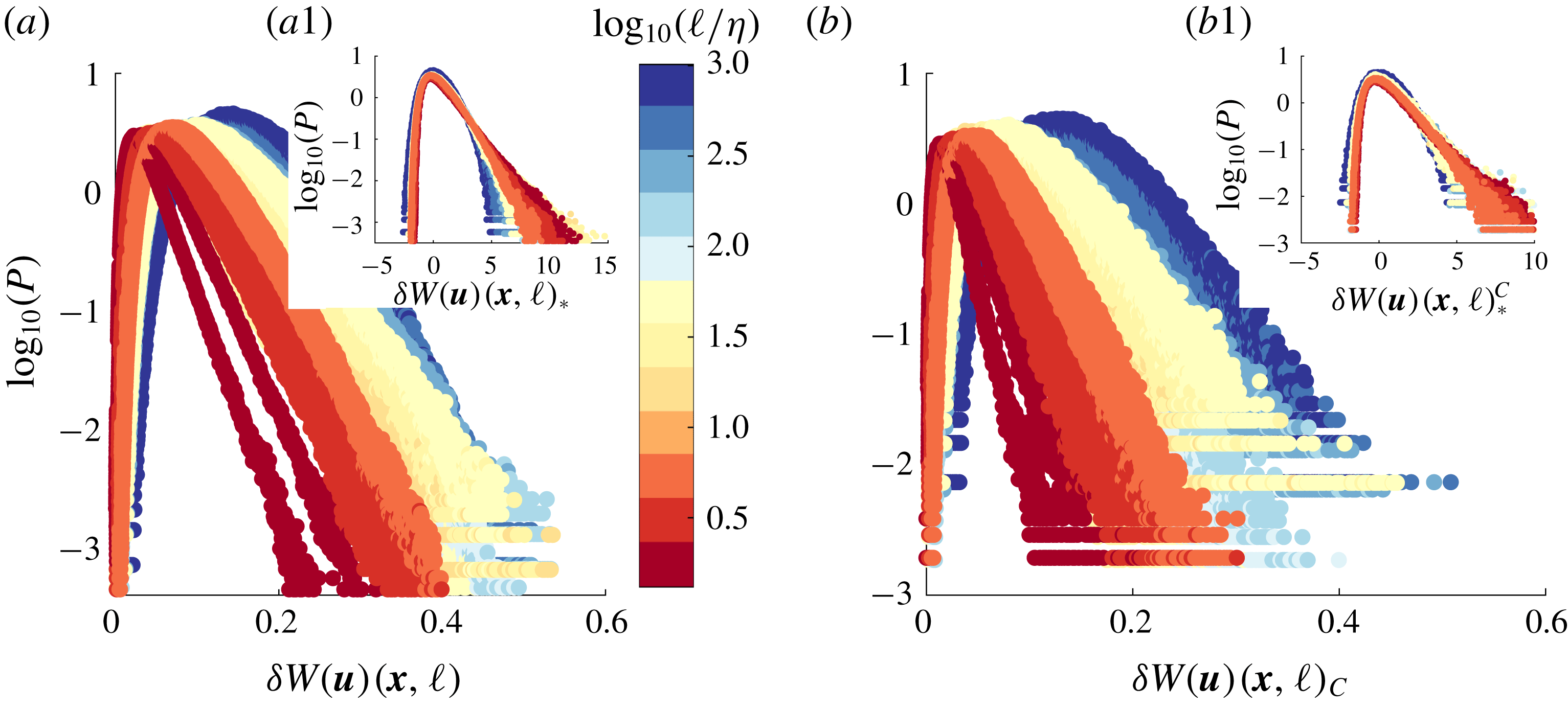
. As shown in figure 10(a), this PDF is non-Gaussian, with fat tails that vary with the scale
 $\ell$
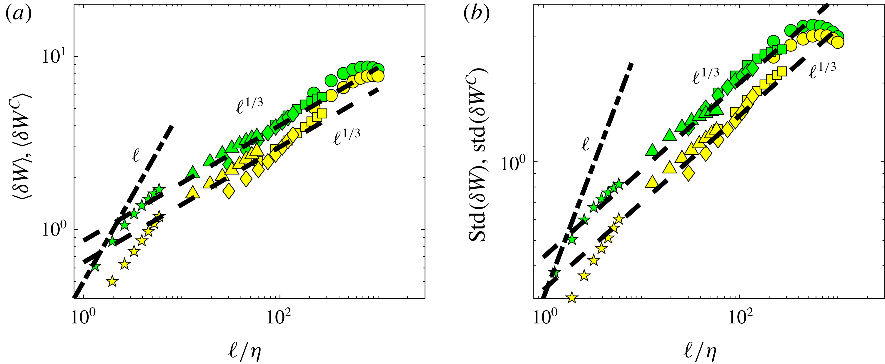
. Both their mean and their standard deviation follow a
 $\ell ^{1/3}$
scaling (figure 11
a) with tiny deviations. This is suggestive of a
 $1/3$
rescaling symmetry. A closer inspection of the ratio of the std to the mean (figure 8
b) shows that it is however not constant, suggesting a breaking of the
 $1/3$
rescaling symmetry. This is confirmed by a plot of centred and reduced PDFs of
 $\unicode[STIX]{x1D6FF}W(\boldsymbol{u})(\boldsymbol{x},\boldsymbol{\ell })$
, that do not collapse on a single curve, as evidenced in figure 10(a1): the tails become wider as the scale decreases, showing that some small-scale process is responsible for the breaking of the
 $1/3$
rescaling symmetry.
PDFs of wavelet velocity increments at different scales, coded by colour, for experiments ANTIG and ANTIC-1 to ANTIC-4 (see figure 11 for corresponding mean and standard deviation and table 1 for symbols). (a) PDF of
 $\unicode[STIX]{x1D6FF}W$
. Inset (a1): centred and reduced PDF of
 $\unicode[STIX]{x1D6FF}W$
at different scales, i.e. PDF of
 $\unicode[STIX]{x1D6FF}W_{\ast }=(\unicode[STIX]{x1D6FF}W-\langle \unicode[STIX]{x1D6FF}W\rangle )/std(\unicode[STIX]{x1D6FF}W)$
. (b) PDF of
 $\unicode[STIX]{x1D6FF}W^{C}$
corresponding to
 $\unicode[STIX]{x1D6FF}W$
conditioned on locations of low values of
 $|\mathscr{D}_{\unicode[STIX]{x0394}x}^{I}|$
. Inset (b1): reduced and centred PDF of
 $\unicode[STIX]{x1D6FF}W^{C}$
.

Scale variation of the mean and standard deviations of the PDFs of wavelet velocity increments for experiments ANTIG and ANTIC-1 to ANTIC-4. (a) Average:
 $\langle \unicode[STIX]{x1D6FF}W\rangle$
: green symbols;
 $\langle \unicode[STIX]{x1D6FF}W^{C}\rangle$
: yellow symbols. (b) Standard deviation
 $std(\unicode[STIX]{x1D6FF}W)$
: green symbols;
 $std(\unicode[STIX]{x1D6FF}W^{C})$
: yellow symbols.

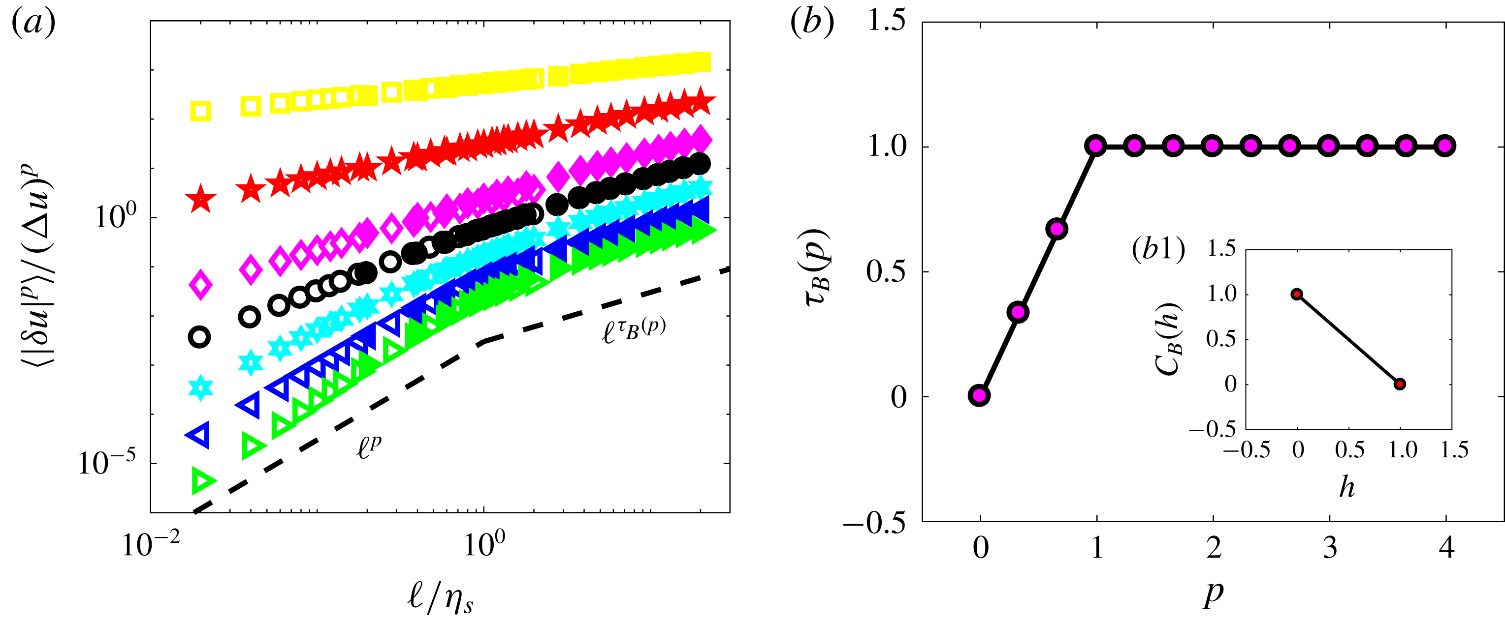
A quantitative measure of this effect is provided by the structure functions
 ${\mathcal{S}}_{p}=\langle (\unicode[STIX]{x1D6FF}W)^{p}\rangle$
. If the
 $1/3$
rescaling symmetry holds exactly, one expects them to be power laws,
 ${\mathcal{S}}_{p}\sim \ell ^{\unicode[STIX]{x1D701}(p)}$
, with
 $\unicode[STIX]{x1D701}(p)=p/3$
. These quantities are plotted in figure 12(a), for
 $p=1$
to
 $6$
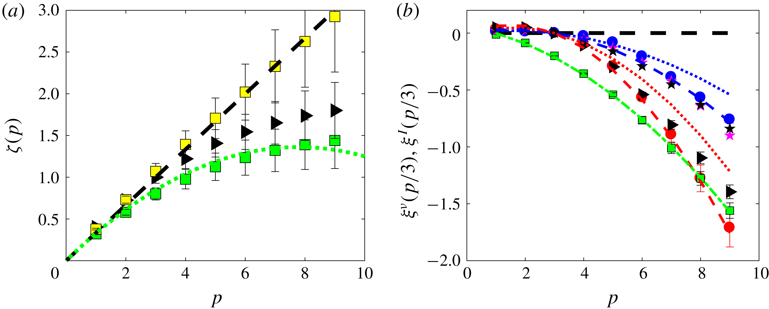
. One sees that they indeed follow a power law with an exponent that is displayed in figure 13(a). It is increasing with
 $p$
and deviates further from the straight line
 $p/3$
as
 $p$
increases. Note that we find
 $\unicode[STIX]{x1D701}(3)=0.8$
and not
 $\unicode[STIX]{x1D701}(3)=1$
that would naively have been expected from K41. Indeed, the prediction of K41 is only for the scaling of the velocity increment of order 3. Here,
 $\unicode[STIX]{x1D701}(3)$
corresponds to the scaling of the absolute value of the wavelet increment. There is no prediction for this quantity in K41. However, we can note that if we consider a rescaled scaling exponent,
 $\unicode[STIX]{x1D701}_{r}(p)=\unicode[STIX]{x1D701}(p)/\unicode[STIX]{x1D701}(3)$
, (this is the exponent we may get by looking at the scaling of
 $S_{p}$
versus
 $S_{3}$
, a technique called extended self-similarity (Benzi et al.
Reference Benzi, Ciliberto, Tripiccione, Baudet, Massaioli and Succi1993)) we guarantee that
 $\unicode[STIX]{x1D701}_{r}(3)=1$
, and we obtain something that appears to be more universal (Arneodo et al.
Reference Arneodo, Baudet, Belin, Benzi, Castaing, Chabaud, Chavarria, Ciliberto, Camussi and Chill1996). The deviation from the Kolmogorov law of the scaling exponent,
 $\unicode[STIX]{x1D709}^{V}=\unicode[STIX]{x1D701}(p)-p/3$
, is shown in figure 17(b). It is well fitted by a parabola.
Such a shape is puzzling, and implies strange pathologies for values of
 $\unicode[STIX]{x1D6FF}W$
that deviates strongly from the mean, as noted in Frisch (Reference Frisch1996). A way to study the behaviour of the distributions of
 $\unicode[STIX]{x1D6FF}W$
is through the function
 $U(p,\ell )=\langle (\unicode[STIX]{x1D6FF}W)^{p+1}\rangle /\langle (\unicode[STIX]{x1D6FF}W)^{p}\rangle$
. Indeed, as
 $p$
increases, this function samples values of
 $\unicode[STIX]{x1D6FF}W$
that deviate increasingly from the mean. Taking into account the observed scaling properties of
 $\unicode[STIX]{x1D6FF}W$
, we get the scaling
 $U(p,\ell )\sim \ell ^{\unicode[STIX]{x0394}(p)}$
with
 $\unicode[STIX]{x0394}(p)=1/3+\unicode[STIX]{x1D709}^{V}(p+1)-\unicode[STIX]{x1D709}^{V}(p)$
which becomes negative as soon as
 $p>p_{\ast }\approx 9$
. This means that if we take first the limit
 $\unicode[STIX]{x1D708}\rightarrow 0$
and then
 $\ell \rightarrow 0$
, the corresponding values
 $U(p>p_{\ast },\ell )$
can take arbitrary large values. This is another indication that the process that is responsible for the breaking of the global symmetry that occurs at small scale, and involves very large values of the velocity gradient, in the limit
 $\unicode[STIX]{x1D708}\rightarrow 0$
. Where does this phenomenon come from?
Scale variation of the non-dimensional wavelet structure function of order
 $p=1$
to
 $p=6$
for experiments ANTIG and ANTIC-1 to ANTIC-4. The structure functions have been shifted by arbitrary factors for clarity and are coded by colour:
 $p=1$
: magenta symbols;
 $p=2$
: green symbols;
 $p=3$
: light blue symbols;
 $p=4$
: red symbols;
 $p=5$
: blue symbols;
 $p=6$
: orange symbols. (a) Structure functions for
 $\unicode[STIX]{x1D6FF}W$
. (b) Structure functions for
 $\unicode[STIX]{x1D6FF}W^{C}$
corresponding to
 $\unicode[STIX]{x1D6FF}W$
conditioned on locations of low values of local energy transfer at the resolution scale
 $|\mathscr{D}_{\unicode[STIX]{x0394}x}^{I}|$
. The dashed lines are power laws with exponents shown in figure 13(a). Adapted from Debue et al. (Reference Debue, Shukla, Kuzzay, Faranda, Saw, Daviaud and Dubrulle2018).

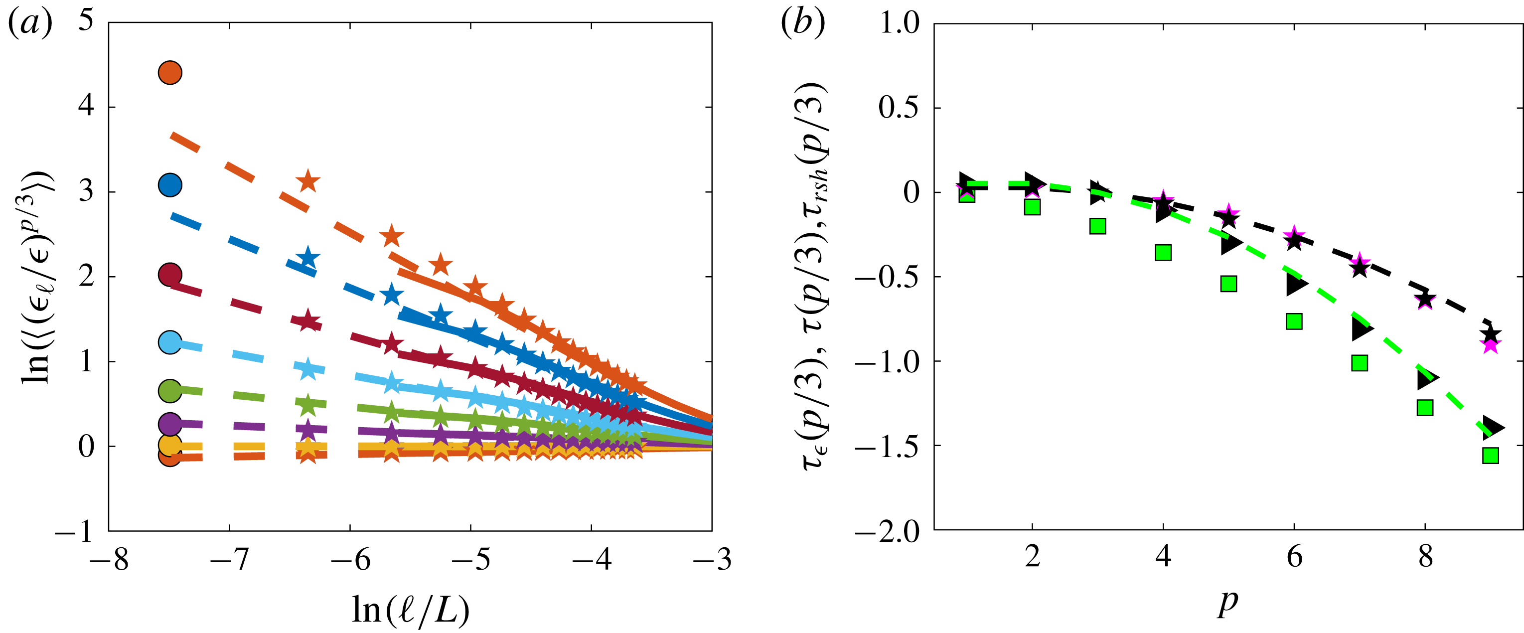
Scaling exponents as a function of order for experiments ANTIG and ANTIC-1 to ANTIC-4. (a) Scaling exponents
 $\unicode[STIX]{x1D701}(p)$
of the wavelet structure functions of
 $\unicode[STIX]{x1D6FF}W$
(green symbols) and
 $\unicode[STIX]{x1D6FF}W^{C}$
(yellow symbols). The exponents have been computed through a least square algorithm upon
 $\unicode[STIX]{x1D701}(p)$
, minimizing the scatter of the non-dimensional structure functions of different experiments with respect to the line
 $(\ell /\unicode[STIX]{x1D702})^{\unicode[STIX]{x1D701}(p)}$
. The green dotted line is the function
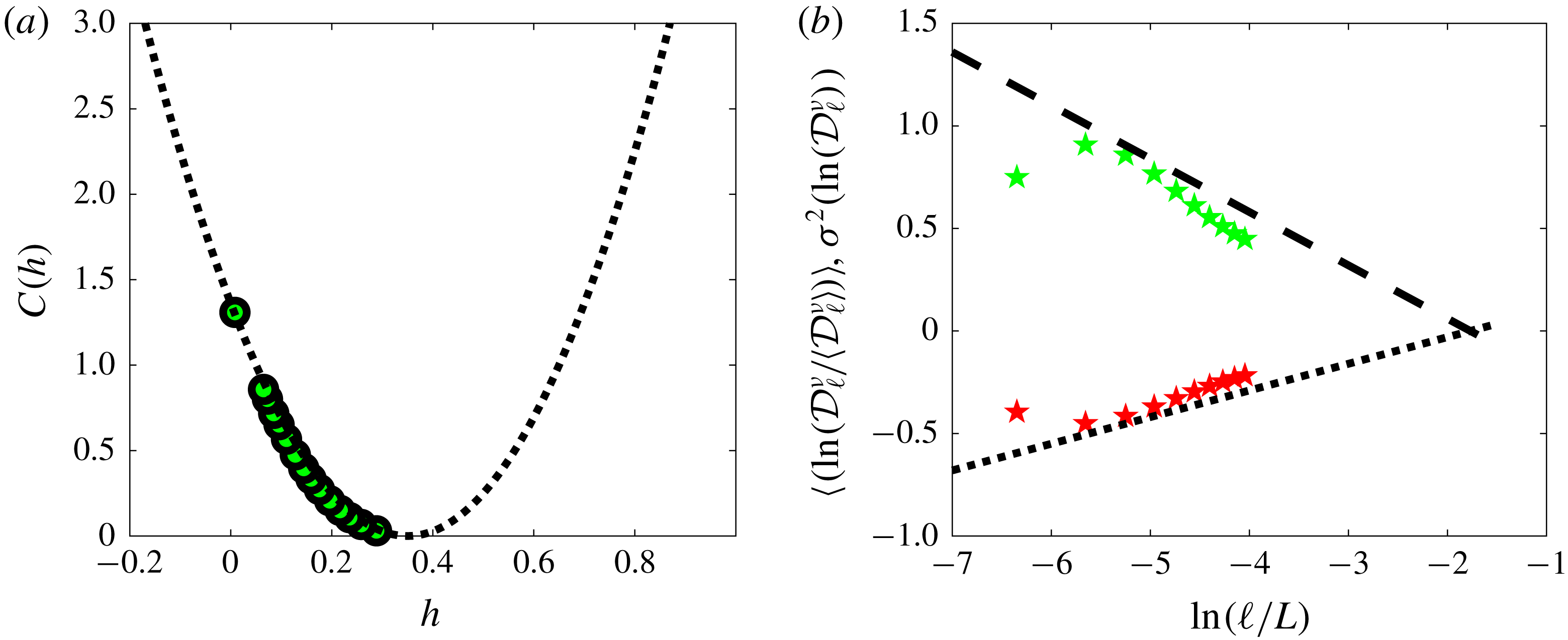
 $\min _{h}(hp+C(h))$
with
 $C(h)$
given in figure 27(a). The black triangles are the rescaled scaling exponents
 $\unicode[STIX]{x1D701}_{r}(p)=\unicode[STIX]{x1D701}(p)/\unicode[STIX]{x1D701}(3)$
. (b) Scaling exponents of the structure function of
 $|\mathscr{D}_{I}^{I}|$
and of
 $|\mathscr{D}_{I}^{\unicode[STIX]{x1D708}}|$
:
 $\unicode[STIX]{x1D709}^{I}(p/3)$
: red circle;
 $\unicode[STIX]{x1D709}^{\unicode[STIX]{x1D708}}(p/3)$
: blue circle. The red dotted (respectively dashed) lines are log-normal fits
 $\unicode[STIX]{x1D709}^{I}(p)=9bp(1-p)/2$
with
 $b=0.045$
(respectively
 $0.065$
). The blue dotted (respectively dashed) lines are log-normal fits
 $\unicode[STIX]{x1D709}^{\unicode[STIX]{x1D708}}(p)=2bp-2bp^{2}$
with
 $b=0.045$
(respectively
 $0.065$
). For comparison, we also reported other scaling exponents:
 $\unicode[STIX]{x1D709}^{V}=\unicode[STIX]{x1D701}(p)-p/3$
(green squares);
 $\unicode[STIX]{x1D70F}_{rsh}=\unicode[STIX]{x1D701}(p)-\unicode[STIX]{x1D701}(3)p/3$
(black triangles);
 $\unicode[STIX]{x1D70F}_{\unicode[STIX]{x1D716}}(p/3)$
for DNS (black stars) and experiment ANTIC-4 (magenta stars), computed from figure 17. The green dot-dashed line is a parabolic fit:
 $\unicode[STIX]{x1D709}^{V}=-0.015p^{2}-0.046p+0.06$
. Adapted from Debue et al. (Reference Debue, Shukla, Kuzzay, Faranda, Saw, Daviaud and Dubrulle2018).

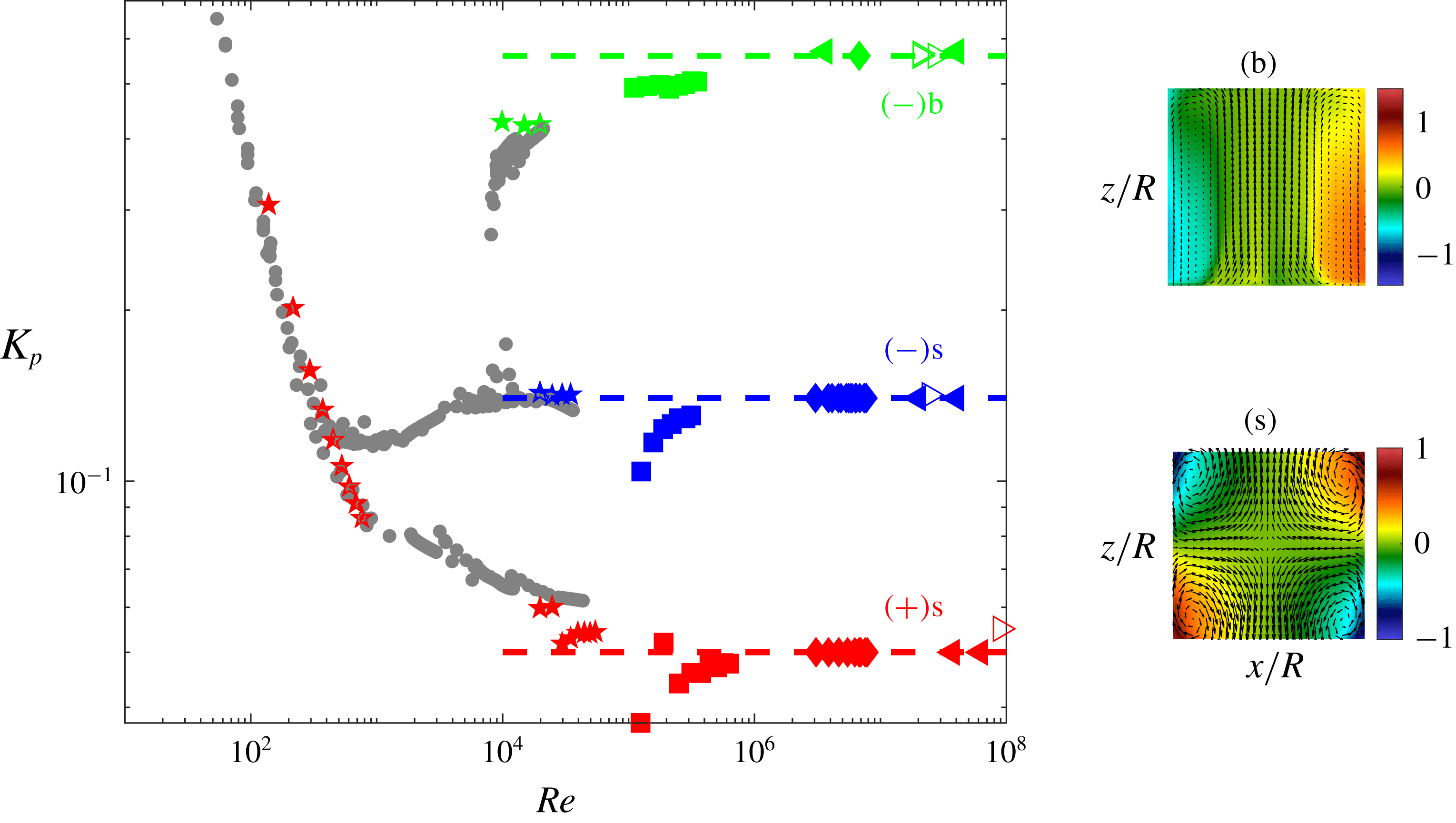
Non-dimensional energy injection rate
 $\unicode[STIX]{x1D716}/2L^{2}\unicode[STIX]{x1D6FA}^{3}$
as a function of Reynolds number
 $Re$
in von Kármán flow using different fluids and different forcings in different experiments. For
 $Re>10^{4}$
, the mean flow is bistable for the
 $(-)$
forcing, and displays two different topologies: (i) a symmetric one, noted (s), shown on the right-south of the main figure; (ii) a non-symmetric one, noted (b) shown on the right-north of the main figure. For a given
 $(-)$
forcing, the energy injection rate is much higher if the flow is in the (b) topology than in the (s) topology. The colour codes the various forcings and flow topologies: red symbols: (
 $+$
) forcing according to figure 1(c), with symmetric mean flow topology; blue and green symbols:
 $(-)$
forcing in respectively symmetric and bifurcated mean flow topology. The symbols code the fluid: pentagons: mixture of water and glycerol, at different concentrations; square: water; diamonds: liquid sodium; left-pointing arrows: helium 4 at
 $T=2.3K$
. Right-pointing arrows: helium 4 at
 $T=2$
K, i.e. in its superfluid phase. The grey symbols are measurements performed in mixture of water and glycerol, with impellers similar to the one shown in figure 1(c), except that they are fitted with 16 blades, instead of 8. The diamonds are unpublished data from the VKS experiment. Courtesy VKS collaboration (M. Faure, N. Bonnefoy, S. Miralles, N. Plihon, J.-F. Pinton, Ph. Odier, G. Verhille, M. Bourgoin, S. Fauve, F. Petrelis, M. Berhanu, N. Mordant, B. Gallet, S. Aumaitre, F. Daviaud, A. Chiffaudel, R. Monchaux, P. Gutierrez). The arrows are obtained from data from the SHREK experiment, with special help from B. Rousset. Adapted from Saint-Michel PhD thesis (Saint-Michel Reference Saint-Michel2013).

4.6 Time-reversal breaking and enstrophy blow up
Let us come back to the enstrophy balance (4.2) – a by-product of the cascade picture – and explore its consequences as we let
 $\unicode[STIX]{x1D708}\rightarrow 0$
. For this, we need to characterize the behaviour of
 $\unicode[STIX]{x1D716}$
, the rate of injected power, as a function of the viscosity
 $\unicode[STIX]{x1D708}$
. In the von Kármán flow (figure 1
b), where the fluid is forced by rotating paddles, this has been done recently using measurements in experiments with the same geometry, but different fluids and tank sizes (Saint-Michel et al.
Reference Saint-Michel, Herbert, Salort, Baudet, Bon Mardion, Bonnay, Bourgoin, Castaing, Chevillard and Daviaud2014). It was found that
 $\unicode[STIX]{x1D716}$
depends on the fluid viscosity
 $\unicode[STIX]{x1D708}$
and on the geometry, size
 $L$
and rotation velocity
 $\unicode[STIX]{x1D6FA}$
of the paddle. However, a remarkable universality appears in the limit of large Reynolds numbers,
 $Re=L^{2}\unicode[STIX]{x1D6FA}/\unicode[STIX]{x1D708}$
, where the flow becomes turbulent. In this limit, the energy injection rate becomes independent of viscosity, and scales like
 $$\begin{eqnarray}\lim _{Re\rightarrow \infty }\unicode[STIX]{x1D716}=2K_{p}L^{2}\unicode[STIX]{x1D6FA}^{3},\end{eqnarray}$$
where
 $K_{p}$
is a parameter that only depends on the geometry of the paddles for a given the topology of the mean flow (figure 14). This universality carries on to the
 $Re=\infty$
limit as proved by recent experiments using super-fluid helium 4 at low temperature (Saint-Michel et al.
Reference Saint-Michel, Herbert, Salort, Baudet, Bon Mardion, Bonnay, Bourgoin, Castaing, Chevillard and Daviaud2014). The behaviour described in (4.8) is well known in the turbulence community and is one of the most robust laws in turbulence. It is sometimes referred to as the zeroth law of turbulence. It is however a rather puzzling law: in the cascade picture, all injected energy is dissipated into heat, i.e. into entropy. Production of entropy is natural in a dissipative system, and is the signature of the breaking of the time-reversal symmetry – in the language of statistical physics, we would call it an order parameter of the time-reversal symmetry. As we have seen in § 4.1, this symmetry is explicitly broken by viscosity. Then, the zeroth law of turbulence means that in a turbulent fluid, at large Reynolds numbers, the order parameter becomes independent of the process that breaks the symmetry. In statistical physics, this behaviour is referred to as a spontaneous symmetry breaking, while in modern field theory language, it is called an anomaly (Falkovich, Gawȩdzki & Vergassola Reference Falkovich, Gawȩdzki and Vergassola2001), so that the constancy of
 $\unicode[STIX]{x1D716}/L^{2}\unicode[STIX]{x1D6FA}^{3}$
is called the dissipation anomaly.
This anomaly has important physical implications in the fluid. When plugged into the enstrophy balance (4.2), it leads to
 $\lim _{\unicode[STIX]{x1D708}\rightarrow 0}\unicode[STIX]{x1D6FA}=\infty$
i.e. enstrophy blow up. This means that there is at least one location in the flow where the vorticity becomes infinite, i.e. that there is a singularity in the flow in the inviscid limit. This conclusion may be disturbing for physicists, but not so much for mathematicians, who have been hunting singularities in the Navier–Stokes equation and its inviscid limit, the Euler equation, for almost a century, starting from Leray (Reference Leray1934). In any case, it is an indication that suitable mathematical tools should be used to understand in greater details the physics of turbulence. This will be the topic of § 6.
Before that, we note that the enstrophy blow up in the inviscid limit is a very strong argument against the universality of small-scale statistics K41 theory, as noted by Landau. Indeed, K41 assumes that everything only depends on the viscosity
 $\unicode[STIX]{x1D708}$
and on
 $\unicode[STIX]{x1D716}$
, the mean energy dissipation rate. The enstrophy blow up in the inviscid limit means that the energy dissipation is subject to large statistical fluctuations that are not necessarily universal, as can be directly observed from figure 6(b1) where the distribution of the energy dissipation displays wide tails. This means that the fluctuations of the energy dissipation cannot be ignored and may break the universality of K41. This remark led Obukhov and Kolmogorov (Reference Kolmogorov1962) to build a ‘refined’ theory (hereafter named K62) that takes explicitly into account these fluctuations.
5 The Kolmogorov–Obukhov refined similarity hypothesis
5.1 Summary of the theory K62
Kolmogorov considers the quantity
 $\unicode[STIX]{x1D716}_{\ell }$
, defined as the viscous dissipation
 $\unicode[STIX]{x1D716}_{\unicode[STIX]{x1D708}}$
averaged over a ball of size
 $\ell$
, and assumes further that
 $\unicode[STIX]{x1D716}_{\ell }$
has a log-normal distribution, with mean and variance of log given by
 $$\begin{eqnarray}\displaystyle & \displaystyle \overline{\unicode[STIX]{x1D716}_{\ell }}=\unicode[STIX]{x1D716},\forall \ell ,\unicode[STIX]{x1D702}\leqslant \ell \leqslant L, & \displaystyle\end{eqnarray}$$
 $$\begin{eqnarray}\displaystyle & \displaystyle \unicode[STIX]{x1D70E}^{2}(\ln (\unicode[STIX]{x1D716}_{\ell }))=-2A-2\unicode[STIX]{x1D707}_{K62}\ln (\ell /L), & \displaystyle\end{eqnarray}$$
where
 $A$
is a non-universal constant that depends on the flow geometry, and
 $\unicode[STIX]{x1D707}_{K62}$
is a universal constant that characterizes the fluctuations. Since the characteristic function of
 $\ln \unicode[STIX]{x1D716}_{\ell }$
gives the moments of
 $\unicode[STIX]{x1D716}$
and is quadratic for a Gaussian, it is straightforward to show that the two hypotheses result in a universal scaling for all moments of
 $\unicode[STIX]{x1D716}_{\ell }$
according to
 $$\begin{eqnarray}\overline{\unicode[STIX]{x1D716}_{\ell }^{p}}\sim \unicode[STIX]{x1D716}^{p}e^{p(1-p)A}\left(\frac{\ell }{L}\right)^{\unicode[STIX]{x1D707}_{K62}p(1-p)}.\end{eqnarray}$$
From this, we can deduce the scaling law of two other interesting quantities:
 $$\begin{eqnarray}\displaystyle & \displaystyle \unicode[STIX]{x1D70E}^{2}(\unicode[STIX]{x1D716}_{\ell })\equiv \overline{\unicode[STIX]{x1D716}_{\ell }^{2}}-\overline{\unicode[STIX]{x1D716}_{\ell }}^{2}=\unicode[STIX]{x1D716}^{2}e^{-2A}\left[\left(\frac{\ell }{L}\right)^{-2\unicode[STIX]{x1D707}_{K62}}-1\right], & \displaystyle\end{eqnarray}$$
 $$\begin{eqnarray}\displaystyle & \displaystyle \overline{\ln (\unicode[STIX]{x1D716}_{\ell })}\equiv \unicode[STIX]{x2202}_{p}(\overline{\unicode[STIX]{x1D716}_{\ell }^{p}})|_{p=0}=\ln (\unicode[STIX]{x1D716})+\unicode[STIX]{x1D707}_{K62}\ln (\ell /L)+A. & \displaystyle\end{eqnarray}$$
Kolmogorov then postulates local universality, so that locally, all quantities only depends on
 $\ell$
,
 $\unicode[STIX]{x1D708}$
and
 $\unicode[STIX]{x1D716}_{\ell }$
. From this, he can define the local velocity scales as
 $U_{\ell }=\ell ^{1/3}\unicode[STIX]{x1D716}_{\ell }^{1/3}$
, dissipative scale
 $\unicode[STIX]{x1D702}_{\ell }=\unicode[STIX]{x1D708}^{3/4}\unicode[STIX]{x1D716}_{\ell }^{-1/4}$
and Reynolds number
 $Re_{\ell }=\ell U_{\ell }/\unicode[STIX]{x1D708}=(\ell /\unicode[STIX]{x1D702}_{\ell })^{4/3}$
. He then obtains
 $$\begin{eqnarray}\displaystyle \overline{\left(\unicode[STIX]{x1D6FF}u_{\ell }\right)^{p}} & = & \displaystyle \overline{\left(\ell \unicode[STIX]{x1D716}_{\ell }\right)^{p/3}}\nonumber\\ \displaystyle & = & \displaystyle C_{p}\left(\ell \unicode[STIX]{x1D716}\right)^{p/3}\left(\frac{\ell }{L}\right)^{\unicode[STIX]{x1D707}_{K62}(1-p/3)p/3}.\end{eqnarray}$$
The scaling of (5.6) means that the global self-similarity is broken, since the rescaled moments
 $\overline{(\unicode[STIX]{x1D6FF}u_{\ell })^{p}}/(\overline{(\unicode[STIX]{x1D6FF}u_{\ell })^{3}})^{p/3}$
scale like
 $\ell ^{\unicode[STIX]{x1D70F}_{K62}(p)}$
with
 $\unicode[STIX]{x1D70F}_{K62}(p)=\unicode[STIX]{x1D707}_{K62}(1-p/3)p/3$
. Moreover, it provides the origin of the symmetry breaking, as resulting from large fluctuations of the local energy dissipation rate over a ball of size
 $\ell$
. In such a process, a new length scale (namely
 $L$
) now appears to play a major role, contributing to scale symmetry breaking.
5.2 Test of refined similarity hypothesis
The refined similarity hypothesis can be tested easily on numerical data. The test with experimental data is more tricky, as it requires measurements of 3 components of velocities at a resolution at least equal to the Kolmogorov scale. Our SPIV data in glycerol are resolved down to the Kolmogorov scale, but they are not rigorously three dimensional, since they are measured only in a plane. They can however be used to compute a pseudo-energy dissipation as
 $\unicode[STIX]{x1D716}_{\unicode[STIX]{x1D708}}=-\unicode[STIX]{x1D708}(\unicode[STIX]{x2202}_{P}\boldsymbol{u})^{2}$
, where
 $\unicode[STIX]{x2202}_{P}$
means the derivative taken only onto the plane of measurements. Given the local instantaneous energy dissipation
 $\unicode[STIX]{x1D716}_{\unicode[STIX]{x1D708}}(\boldsymbol{x},t)$
, an estimate of
 $\unicode[STIX]{x1D716}_{\ell }$
is through a convolution through the smoothing function we used for wavelets
 $$\begin{eqnarray}\displaystyle & \displaystyle \unicode[STIX]{x1D716}_{\ell }(\boldsymbol{x},t)=\int \text{d}\boldsymbol{r}\,\unicode[STIX]{x1D6F7}_{\ell }(\boldsymbol{r})\unicode[STIX]{x1D716}_{\unicode[STIX]{x1D708}}(\boldsymbol{x}+\boldsymbol{r},t), & \displaystyle\end{eqnarray}$$
 $$\begin{eqnarray}\displaystyle & \displaystyle \unicode[STIX]{x1D716}_{\unicode[STIX]{x1D708}}(\boldsymbol{x},t)=\unicode[STIX]{x1D708}\left(\unicode[STIX]{x2202}u\right)^{2}(x,t). & \displaystyle\end{eqnarray}$$
Observe that for
 $\ell \rightarrow 0$
,
 $\unicode[STIX]{x1D716}_{\ell }\rightarrow \unicode[STIX]{x1D716}_{\unicode[STIX]{x1D708}}$
and that for
 $\ell \rightarrow L$
(
 $L$
being the size of the volume containing the fluid),
 $\unicode[STIX]{x1D716}_{\ell }\rightarrow P_{diss}/\unicode[STIX]{x1D70C}L^{3}$
, the instantaneous energy dissipation rate.
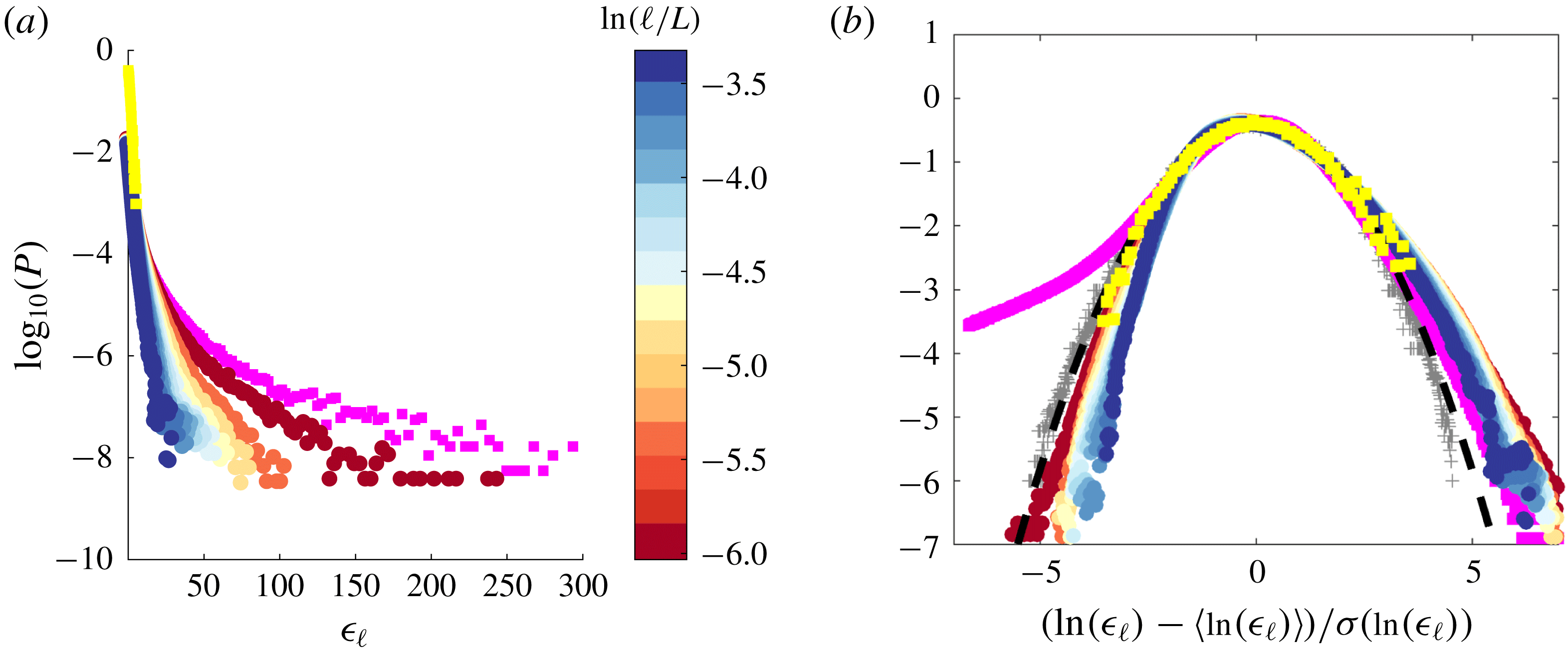
Probability distribution functions of the pseudo-energy dissipation averaged over a ball of size
 $\ell$
in experiment ANTIC-4 at various scales
 $\ell /L$
, coded by colour (see colour bar). The magenta squares are for the non-averaged pseudo-dissipation
 $\unicode[STIX]{x1D716}_{\unicode[STIX]{x1D708}}$
. The yellow symbols, for the time averaged pseudo-dissipation
 $P_{diss}/\unicode[STIX]{x1D70C}L^{3}$
. (a) PDF of
 $\unicode[STIX]{x1D716}_{\ell }$
. (b) Centred reduced PDF of
 $\ln (\unicode[STIX]{x1D716}_{\ell })$
. The black dashed line is a log-normal with zero mean and unit variance. The grey crosses are centred and reduced distributions of
 $\unicode[STIX]{x1D716}_{\ell }$
in DNS A, at scales corresponding to
 $\ell /L=0$
and
 $\ell /L=n\unicode[STIX]{x1D702}/L$
, with
 $n=1,3$
and
 $10$
.

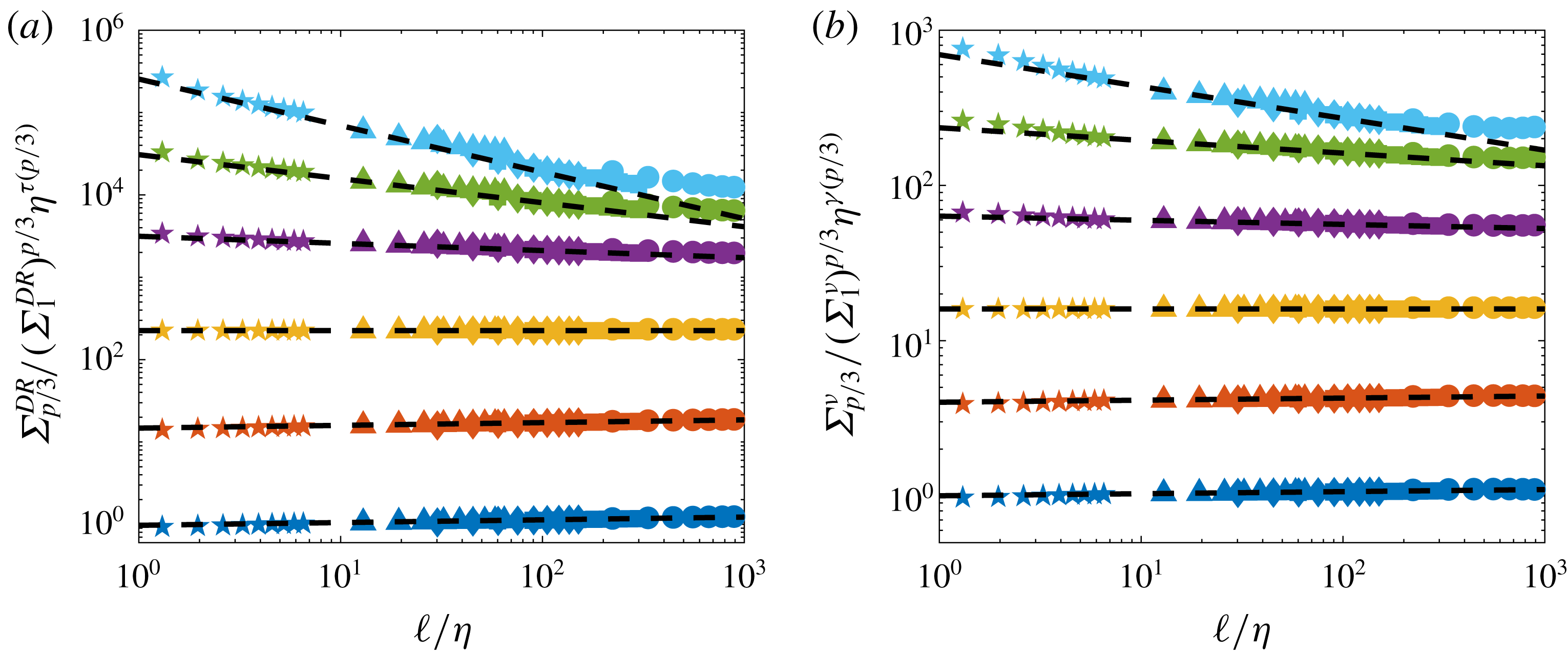
The PDF of the resulting distributions, for various
 $\ell$
, is provided in figure 15(a), along with the distributions of
 $\unicode[STIX]{x1D716}_{\unicode[STIX]{x1D708}}$
and
 $P_{diss}/\unicode[STIX]{x1D70C}L^{3}$
. One sees that they vary widely in shape, as
 $\ell$
is varied, with a variance decreasing as scale is increased. To test the hypothesis of K62, we compute the PDF of
 $\ln (\unicode[STIX]{x1D716}_{\ell })$
for various
 $\ell /L$
, shown in figure 15(b). They are indeed close to parabolic, with deviations that could be due noise or projection effect. By comparison, the PDF of
 $\ln (\unicode[STIX]{x1D716}_{\ell })$
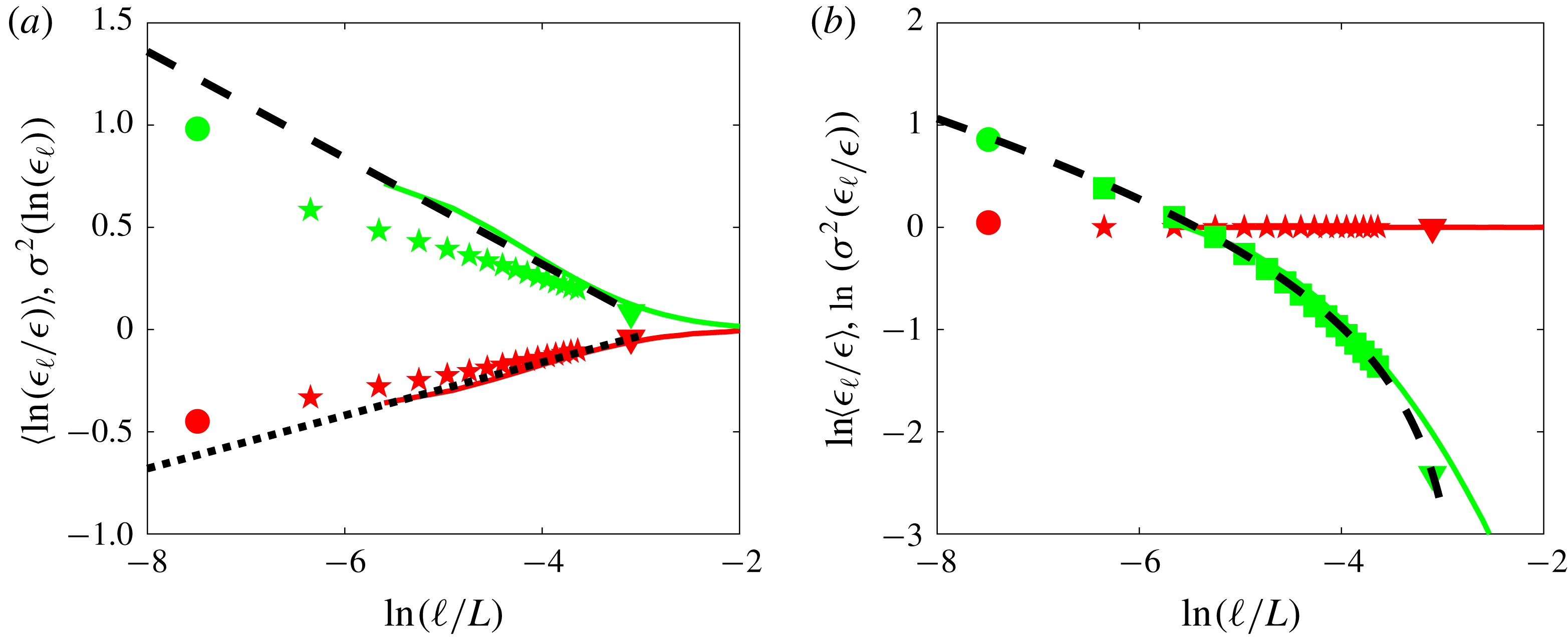
for the numerical simulation DNS A is indeed perfectly parabolic, for all scales. To investigate the accuracy of K62 to describe the data, we compute the mean and variances of
 $\unicode[STIX]{x1D716}_{\ell }$
and
 $\ln \unicode[STIX]{x1D716}_{\ell }$
and plot them as a function of
 $\ell /L$
in figure 16(a,b), for both numerical and experimental data. The average of
 $\unicode[STIX]{x1D716}_{\ell }$
is indeed constant (equation (5.1)), while its variance decreases and is well described by (5.4) using
 $\unicode[STIX]{x1D707}=0.13$
and
 $A=0.36$
. With these two numbers, we can then fit the mean and variances of
 $\ln (\unicode[STIX]{x1D716}_{\ell })$
using (5.5) and (5.2) without adjusting parameters. We see that the fit is fair for experiments, but rather good for the numerical data.
Mean (red symbols) and variances (green symbols) of PDF of (a)
 $\unicode[STIX]{x1D716}_{\ell }$
and (b)
 $\ln (\unicode[STIX]{x1D716}_{\ell })$
in experiment ANTIC-4 as a function of scale
 $\ell /L$
: circle:
 $\unicode[STIX]{x1D716}_{\unicode[STIX]{x1D708}}$
; stars:
 $\unicode[STIX]{x1D716}_{\ell }$
; triangles:
 $P_{diss}/\unicode[STIX]{x1D70C}L^{3}$
. In (a), the dashed line is a fit using the shape given by (5.4), with
 $\unicode[STIX]{x1D707}_{K62}=0.13$
and
 $A=0.36$
. These two numbers are then used to compute the dotted (respectively the dashed line) in (b), via (5.5) (respectively (5.2)). The coloured full lines are obtained using DNS A.

Consistency with K62 can be further checked by computing moments of higher order for
 $\unicode[STIX]{x1D716}_{\ell }$
as a function of
 $\ell$
. They are reported in figure 17(a). In the inertial range
 $\ln (\ell /\unicode[STIX]{x1D702})\geqslant 4$
, they follow the power law
 $\langle (\unicode[STIX]{x1D716}_{\ell })^{p/3}\rangle \sim \unicode[STIX]{x1D716}^{p/3}\ell ^{\unicode[STIX]{x1D70F}_{\unicode[STIX]{x1D716}}(p/3)}$
, with
 $\unicode[STIX]{x1D70F}_{\unicode[STIX]{x1D716}}(p/3)$
reported in figure 17(b) for both experiments and DNS. They are parabolic, as suggested by K62, and well fitted by the exact log-normal shape
 $\unicode[STIX]{x1D70F}_{\unicode[STIX]{x1D716}}(p/3)=\unicode[STIX]{x1D707}_{K62}(1-p/3)p/3$
, with
 $\unicode[STIX]{x1D707}_{K62}=0.13$
. The moments
 $\langle (\unicode[STIX]{x1D716}_{\ell })^{p/3}\rangle$
can also be well fitted without any adjustable parameter by (5.3), with
 $\unicode[STIX]{x1D707}_{K62}$
and
 $A$
computed using the variance of
 $\ln (\unicode[STIX]{x1D716}_{\ell })$
. From all this, we see that the log-normal hypothesis formulated by Kolmogorov is fairly well satisfied by numerical and experimental data.
However, when we compare
 $\unicode[STIX]{x1D70F}_{\unicode[STIX]{x1D716}}(p/3)$
and
 $\unicode[STIX]{x1D709}^{V}=\unicode[STIX]{x1D701}(p)-p/3$
computed from the wavelet analysis in § 4.5, we observe a rather large discrepancy, in contradiction with the Kolmogorov refined similarity hypothesis (5.6). We can argue that the problem is due to the fact that
 $\unicode[STIX]{x1D701}(3)$
is not equal to one (see § 4.5), meaning that
 $\unicode[STIX]{x1D709}^{V}(1)$
is not zero, as necessary in the refined scaling hypothesis. We may correct that by using
 $\unicode[STIX]{x1D70F}_{rsh}(p/3)=\unicode[STIX]{x1D701}(p)-\unicode[STIX]{x1D701}(3)p/3$
, which is indeed closer to
 $\unicode[STIX]{x1D70F}_{\unicode[STIX]{x1D716}}(p/3)$
, but there is still a discrepancy. Where does the problem come from?
Test of refined similarity hypothesis. (a) Structure functions of
 $\unicode[STIX]{x1D716}_{\ell }$
as a function of
 $\ell /L$
in experiment ANTIC-4 (symbols):
 $\ell /L$
: circle:
 $\unicode[STIX]{x1D716}_{\unicode[STIX]{x1D708}}$
; stars:
 $\unicode[STIX]{x1D716}_{\ell }$
; triangles:
 $P_{diss}/\unicode[STIX]{x1D70C}L^{3}$
, and in DNS A (continuous line). The structure functions are coded by colour:
 $p=1$
: blue;
 $p=2$
: orange;
 $p=3$
: yellow;
 $p=4$
: magenta;
 $p=5$
: green;
 $p=6$
: light blue;
 $p=7$
: red;
 $p=8$
: blue;
 $p=9$
: orange. The coloured dashed lines are (5.3), with
 $\unicode[STIX]{x1D707}_{K62}$
and
 $A$
computed using variance of
 $\ln (\unicode[STIX]{x1D716}_{\ell })$
. (b) Scaling exponents of the structure functions:
 $\unicode[STIX]{x1D70F}_{\unicode[STIX]{x1D716}}(p/3)$
for experiment ANTIC-4 (magenta stars); for DNS A (black stars). The black dashed line is
 $\unicode[STIX]{x1D707}_{K62}(1-p/3)p/3$
, with
 $\unicode[STIX]{x1D707}_{K62}=0.13$
, obtained in figure 16. These values do not coincide with the quantity
 $\unicode[STIX]{x1D70F}(p/3)=\unicode[STIX]{x1D701}(p)-p/3$
(green squares), and
 $\unicode[STIX]{x1D70F}_{rsh}(p/3)=\unicode[STIX]{x1D701}(p)-\unicode[STIX]{x1D701}(3)p/3$
(black triangles) inferred from figure 13(a) using directly wavelet velocity increments, that are best fitted (green dotted line) by
 $\unicode[STIX]{x1D707}(1-p/3)p/3$
with
 $\unicode[STIX]{x1D707}=0.24>\unicode[STIX]{x1D707}_{K62}$
, in contradiction with K62.

5.3 Problems and issues set by K62
Let us come back to the mathematics behind K62. In the Kolmogorov cascade picture, the energy is transferred locally from a scale
 $\ell$
to a scale
 $\unicode[STIX]{x1D6E4}\ell$
(
 $\unicode[STIX]{x1D6E4}\leqslant 1$
) in a self-similar way, so that the distribution of
 $\unicode[STIX]{x1D716}_{\ell }/\unicode[STIX]{x1D716}_{\unicode[STIX]{x1D6E4}\ell }$
only depends on the ratio of scales
 $\unicode[STIX]{x1D6E4}$
. Writing
 $\unicode[STIX]{x1D716}_{L}/\unicode[STIX]{x1D716}_{\unicode[STIX]{x1D6E4}^{N}L}=(\unicode[STIX]{x1D716}_{L}/\unicode[STIX]{x1D716}_{\unicode[STIX]{x1D6E4}L})\cdots (\unicode[STIX]{x1D716}_{\unicode[STIX]{x1D6E4}^{N-1}L}/\unicode[STIX]{x1D716}_{\unicode[STIX]{x1D6E4}^{N}L})$
, we see that for any
 $\ell =\unicode[STIX]{x1D6E4}^{N}L$
, the quantity
 $\ln (\unicode[STIX]{x1D716}_{\ell }/\unicode[STIX]{x1D716}_{L})$
is the sum of
 $N=\ln (L/\ell )/\ln (\unicode[STIX]{x1D6E4})$
variables with identical distributions
 $$\begin{eqnarray}\ln (\unicode[STIX]{x1D716}_{\ell }/\unicode[STIX]{x1D716}_{L})=\unicode[STIX]{x1D6F4}_{n=1}^{\ln (L/\ell )/\ln (\unicode[STIX]{x1D6E4})}\ln (\unicode[STIX]{x1D716}_{\unicode[STIX]{x1D6E4}^{n}L}/\unicode[STIX]{x1D716}_{\unicode[STIX]{x1D6E4}^{n-1}L}).\end{eqnarray}$$
When
 $N=\ln (L/\ell )/\ln (\unicode[STIX]{x1D6E4})\rightarrow \infty$
, and if the distributions are independent, we can then use large deviation theory (Kramer’s theorem) (Touchette Reference Touchette2009) to write the probability of observing
 $\ln (\unicode[STIX]{x1D716}_{\ell }/\unicode[STIX]{x1D716}_{L})$
as
 $$\begin{eqnarray}P(\ln (\unicode[STIX]{x1D716}_{\ell }/\unicode[STIX]{x1D716}_{L})=x)\sim \text{e}^{-NF(x/N)},\end{eqnarray}$$
where
 $F$
is the large deviation function that only depends on the distribution of
 $\unicode[STIX]{x1D716}_{\ell }/\unicode[STIX]{x1D716}_{\unicode[STIX]{x1D6E4}\ell }$
. The highest probability (the most likely event) is obtained for the value
 $x$
that is connected to the
 $z^{\ast }$
, the location of the maximum value of
 $F$
, via
 $x=Nz^{\ast }$
. For values of
 $x/N$
close to
 $z^{\ast }$
, the function
 $F$
is parabolic, so that
 $F(z)=F(z^{\ast })+F^{\prime \prime }(z^{\ast })(z-z^{\ast })^{2}/2$
and
 $$\begin{eqnarray}P\left(\ln (\unicode[STIX]{x1D716}_{\ell }/\unicode[STIX]{x1D716}_{L})=x\approx z^{\ast }\ln (L/\ell )\right)\sim \text{e}^{-NF(z^{\ast })-(F^{\prime \prime }(z^{\ast })/N)(x-Nz^{\ast })^{2}/2},\end{eqnarray}$$
corresponding to a log-normal distribution for
 $\unicode[STIX]{x1D716}/\unicode[STIX]{x1D716}_{L}$
, with a variance
 $\ln (L/\ell )/F^{\prime \prime }(z^{\ast })$
. This is K62 theory, with
 $\unicode[STIX]{x1D707}_{K62}\propto 1/F^{\prime \prime }(z^{\ast })$
. However, for values far from the most probable value, the large deviation function
 $F$
can differ from a parabola, and deviation from log-normal can be observed.
This argument is only valid provided the distributions of
 $\unicode[STIX]{x1D716}_{\unicode[STIX]{x1D6E4}^{p-1}\ell }/\unicode[STIX]{x1D716}_{\unicode[STIX]{x1D6E4}^{p}\ell }$
for different
 $p$
are independent. If they are correlated, no general prediction about their sum can be given (see Clusel & Bertin (Reference Clusel and Bertin2008) for solvable examples), and one can obtain shapes different from log-normal. We thus see that the K62 theory is based on an idealized treatment of the fluctuations that does not necessarily reflect reality.
Another questionable assumption holds in the interpretation of (5.6), that allows us to connect the velocity structure function to the quantity
 $\unicode[STIX]{x1D716}_{\ell }$
. Indeed, in the original K41 theory,
 $\unicode[STIX]{x1D716}_{\ell }$
was inferred from KHM equation as the constant scale-to-scale energy transfer. This remark led Kraichnan (Reference Kraichnan1974) to suggest that if such a relation holds,
 $\unicode[STIX]{x1D716}_{\ell }$
should represent some well-defined local energy flux
 $\unicode[STIX]{x1D6F1}_{\ell }$
rather than a local energy dissipation averaged over a volume of linear dimension
 $\ell$
. Since K62 is not derived directly from the Navier–Stokes equations, it is not obvious how to define precisely the expression and properties of
 $\unicode[STIX]{x1D6F1}_{\ell }$
. To make further progress, we need to find a generalization of K41 that (i) provides and expression of such local energy flux; (ii) does not suffer from the main drawbacks of K41, namely that does not assumes homogeneity, nor stationarity, that allow for breaking of the time symmetry and (iii) takes into account the fluctuations of energy dissipation and allows for the breaking of the self-similarity. This generalization was derived in 1990 by two French mathematicians, Duchon and Robert. The purpose of the next section is to summarize their derivation, and explore its outcomes.
6 Weak formulation of Kármán–Howarth–Monin equation
6.1 Derivation of the weak Kármán–Howarth–Monin equation
6.1.1 Why a weak formulation?
In previous sections, we have identified many clues about a pathological behaviour of the velocity field in turbulent flows: development of large gradients, inhomogeneity and intermittency of the dissipation, spontaneous breaking of the time-reversal
 $\text{symmetry}\ldots$
. Even the simple Kolmogorov picture involves lack of regularity for the velocity field. Indeed, we have
 $$\begin{eqnarray}|\overline{\langle (\unicode[STIX]{x1D6FF}\boldsymbol{u})^{3}\rangle }|\leqslant \overline{\langle |\unicode[STIX]{x1D6FF}\boldsymbol{u}|^{3}\rangle }.\end{eqnarray}$$
Let us further assume that there exist an
 $h$
and a
 $C$
, such that
 $\forall x$
and
 $\ell \leqslant \ell _{0}$
 $$\begin{eqnarray}|\unicode[STIX]{x1D6FF}\boldsymbol{u}|\leqslant C\ell ^{h}.\end{eqnarray}$$
In mathematical language, this means that the velocity field is uniform Hölder continuous with exponent
 $h$
. Substituting in (6.1), we then see that
 $$\begin{eqnarray}|\overline{\langle (\unicode[STIX]{x1D6FF}\boldsymbol{u})^{3}\rangle }|\leqslant C^{3}\ell ^{3h},\end{eqnarray}$$
so that Kolmogorov scaling cannot be satisfied if
 $h>1/3$
, because
 $\overline{\langle (\unicode[STIX]{x1D6FF}\boldsymbol{u})^{3}\rangle }$
will tend to zero always faster than
 $\ell$
. This means that there is at least one point in the flow where the inequality (6.2) with
 $h>1/3$
is violated, possibly satisfied only with some
 $h\leqslant 1/3$
. At such a point, the field is irregular, since velocity gradients can blow up like
 $\ell ^{h-1}$
in the limit
 $\ell \rightarrow 0$
. We call such fields ‘rough’, in opposition to ‘smooth’ fields, characterized by a Hölder continuous exponent
 $h=1$
everywhere.
Rough fields are delicate to deal with, especially in the context of partial differential equations such as the Navier–Stokes equations, because derivatives are not necessarily well behaved. A suitable tool to deal with them was invented by Leray (Reference Leray1934) and named ‘weak formulation’. The main idea is to make a detour via the scale space, and work with a smoothed version of the initial field (a ‘mollified’ field), over a characteristic scale (resolution)
 $\ell$
. At any given resolution
 $\ell$
, the mollified field is sufficiently regular, so that all classical tools and the manipulation of the analysis of vector fields are valid. Limiting behaviours as the resolution
 $\ell \rightarrow 0$
can then be used to infer results and properties for the rough field.
6.1.2 How to implement a weak formulation?
The implementation of a weak formulation requires the introduction of a smoothing operator (or test function)
 $\unicode[STIX]{x1D719}(x)$
, with suitable properties: it must be smooth (at least twice differentiable for Navier–Stokes) with compact support on
 $\mathbb{R}^{3}$
, even, non-negative, spatially localized and such that
 $\int \text{d}\boldsymbol{r}\,\unicode[STIX]{x1D719}(\boldsymbol{r})=1$
. The smoothing at a resolution
 $\ell$
is then achieved through the function
 $\unicode[STIX]{x1D719}_{\ell }$
, defined as
 $\unicode[STIX]{x1D719}_{\ell }(\boldsymbol{r})=\ell ^{-3}\unicode[STIX]{x1D719}\left(\boldsymbol{r}/\ell \right)$
. For any given rough field
 $\boldsymbol{u}(\boldsymbol{x},t)$
, the mollified field is defined as
 $$\begin{eqnarray}u_{i}^{\ell }(\boldsymbol{x},t)=\int \text{d}\boldsymbol{r}\,\unicode[STIX]{x1D719}_{\ell }(\boldsymbol{r})u_{i}(\boldsymbol{x}+\boldsymbol{r},t).\end{eqnarray}$$
The properties of
 $\unicode[STIX]{x1D719}$
guarantee that when
 $\ell \rightarrow 0$
,
 $u_{i}^{\ell }\rightarrow u_{i}$
. Moreover, the velocity derivative of the rough field
 $u_{i}$
can be written as
 $$\begin{eqnarray}\unicode[STIX]{x2202}_{j}u_{i}^{\ell }(\boldsymbol{x},t)=-\lim _{\ell \rightarrow 0}\int \text{d}\boldsymbol{r}\,\unicode[STIX]{x2202}_{j}\unicode[STIX]{x1D719}_{\ell }(\boldsymbol{r})u_{i}(\boldsymbol{x}+\boldsymbol{r},t),\end{eqnarray}$$
as well as any higher-order derivative of
 $u_{i}$
, as long as
 $\unicode[STIX]{x1D719}$
is sufficiently regular.
The weak formalism has some interesting connections with classical tools of turbulence. First, equation (6.4) shows that the mollifying process is a coarse graining. As such, it averages out fine details about the fields while keeping information about large scales. Formally, the mollified velocity can also be seen as a continuous wavelet transform of the velocity
 $\boldsymbol{u}$
with respect to the wavelet
 $\unicode[STIX]{x1D719}$
. Note, however, that since we have chosen
 $\unicode[STIX]{x1D719}$
to be of unit integral, it is not admissible, meaning that the wavelet transform is not invertible.
6.1.3 Advantages of the weak formulation
The link between the weak formulation and wavelet transform unveils several advantages of its application to turbulent rough fields. A wavelet transform is a kind of ‘local Fourier transform’. As such, it is more suitable for application onto non-homogeneous fields and will naturally deal with the observed breaking of the space translation symmetry (§ 4.3). A wavelet transform is also by construction ‘locally self-similar’. It is therefore the relevant tool to measure local Hölder exponents, as proved by Arneodo and his group (Muzy et al.
Reference Muzy, Bacry and Arneodo1991). Specifically, it can be shown that if a field is locally Hölder continuous with exponent
 $h$
around
 $\boldsymbol{x}_{0}$
, then its wavelet transform will scale locally like
 $|u_{i}^{\ell }(\boldsymbol{x}_{0},t)|\sim \ell ^{h}$
. (Rigorously, this is valid only when the wavelet has enough vanishing moments, namely more than the degree of a local polynomial corresponding to the regular part of the Taylor expansion of
 $u$
near
 $x_{0}$
.) This means that the weak formulation will be able to keep track of the global-scale symmetry and its violations (§ 4.5)).
I hope that the reader is now convinced that the weak formulation, and its associated continuous wavelet transform, is the natural tool to generalize the KHM equation into a ‘local’ version, that will help to go beyond K41 and K62. Let us now summarize the main steps of Duchon and Robert’s derivation (Duchon & Robert Reference Duchon and Robert2000).
6.1.4 Summary of Duchon–Robert derivation
We first apply the wavelet transform to the Navier–Stokes equations (1.1), to get a classical coarse-grained equation
 $$\begin{eqnarray}\unicode[STIX]{x2202}_{t}u_{i}^{\ell }+u_{j}^{\ell }\unicode[STIX]{x2202}_{j}u_{i}^{\ell }=-\unicode[STIX]{x2202}_{j}\unicode[STIX]{x1D70F}_{ij}^{\ell }-\frac{1}{\unicode[STIX]{x1D70C}}\unicode[STIX]{x2202}_{i}p^{\ell }+\unicode[STIX]{x1D708}\unicode[STIX]{x2202}_{jj}u_{i}^{\ell },\end{eqnarray}$$
where
 $\unicode[STIX]{x1D70F}_{ij}^{\ell }=(u_{i}u_{j})^{\ell }-u_{i}^{\ell }u_{j}^{\ell }$
is the classical Reynolds stress tensor. We multiply (1.1) and (6.6) by
 $\boldsymbol{u}^{\ell }$
and
 $\boldsymbol{u}$
, respectively, and add them together; after the rearrangement of terms we obtain the following balance equation:
 $$\begin{eqnarray}\unicode[STIX]{x2202}_{t}u_{i}u_{i}^{\ell }+\unicode[STIX]{x2202}_{i}T_{i}={\mathcal{E}}^{\ell }+\unicode[STIX]{x1D708}u_{i}\unicode[STIX]{x2202}^{2}u_{i}^{\ell }+\unicode[STIX]{x1D708}u_{i}^{\ell }\unicode[STIX]{x2202}^{2}u_{i},\end{eqnarray}$$
where
 $$\begin{eqnarray}\displaystyle \left.\begin{array}{@{}c@{}}\displaystyle T_{i}=u_{j}u_{j}^{\ell }u_{i}+(p^{\ell }u_{i}+pu_{i}^{\ell })/\unicode[STIX]{x1D70C},\\ \displaystyle {\mathcal{E}}^{\ell }=u_{i}u_{j}\unicode[STIX]{x2202}_{i}u_{j}^{\ell }-u_{j}\unicode[STIX]{x2202}_{i}(u_{i}u_{j})^{\ell }.\end{array}\right\} & & \displaystyle\end{eqnarray}$$
Developing terms and using properties of
 $\unicode[STIX]{x1D719}$
, it is simple to check that
 ${\mathcal{E}}^{\ell }$
can be split into
 $$\begin{eqnarray}2{\mathcal{E}}^{\ell }=-\unicode[STIX]{x2202}_{i}(u_{i}u_{j}u_{j})^{\ell }+\unicode[STIX]{x2202}_{i}(u_{i}(u_{j}u_{j})^{\ell })-\int \text{d}\unicode[STIX]{x1D743}\,\unicode[STIX]{x1D735}\unicode[STIX]{x1D719}^{\ell }(\unicode[STIX]{x1D743})\boldsymbol{\cdot }\unicode[STIX]{x1D6FF}_{\unicode[STIX]{x1D709}}\boldsymbol{u}(\unicode[STIX]{x1D6FF}_{\unicode[STIX]{x1D709}}\boldsymbol{u})^{2},\end{eqnarray}$$
where
 $\unicode[STIX]{x1D6FF}_{\unicode[STIX]{x1D709}}\boldsymbol{u}$
is the velocity increment over a distance
 $\unicode[STIX]{x1D743}$
and
 $\unicode[STIX]{x1D735}$
the gradient over
 $\unicode[STIX]{x1D743}$
. We can also split
 $$\begin{eqnarray}u_{i}^{\ell }\unicode[STIX]{x2202}^{2}u_{i}=\unicode[STIX]{x2202}_{j}(u_{i}^{\ell }\unicode[STIX]{x2202}_{j}u_{i}-u_{i}\unicode[STIX]{x2202}_{j}u_{i}^{\ell })+u_{i}\unicode[STIX]{x2202}^{2}u_{i}^{\ell }.\end{eqnarray}$$
Finally, it is straightforward to check that
 $$\begin{eqnarray}\frac{1}{2}\int \text{d}\unicode[STIX]{x1D743}\,\unicode[STIX]{x1D6FB}^{2}\unicode[STIX]{x1D719}^{\ell }(\unicode[STIX]{x1D743})(\unicode[STIX]{x1D6FF}_{\unicode[STIX]{x1D709}}\boldsymbol{u})^{2}=\frac{1}{2}\unicode[STIX]{x2202}^{2}(u_{i}u_{i})^{\ell }-u_{i}\unicode[STIX]{x2202}^{2}u_{i}^{\ell }.\end{eqnarray}$$
After the rearrangement of terms, we finally get a local balance equation for the quantity
 $E^{\ell }(\boldsymbol{x})\equiv u_{i}u_{i}^{\ell }/2$
as
 $$\begin{eqnarray}\unicode[STIX]{x2202}_{t}E^{\ell }(\boldsymbol{x})+\unicode[STIX]{x2202}_{j}J_{j}=-\mathscr{D}_{\ell }^{I}-\mathscr{D}_{\ell }^{\unicode[STIX]{x1D708}},\end{eqnarray}$$
where
 $$\begin{eqnarray}\displaystyle & \displaystyle J_{i}=u_{i}E^{\ell }+{\textstyle \frac{1}{2}}(p^{\ell }u_{i}+pu_{i}^{\ell })+{\textstyle \frac{1}{4}}([u_{i}u_{j}u_{j}]^{\ell }-u_{i}[u_{j}u_{j}]^{\ell })-\unicode[STIX]{x1D708}\unicode[STIX]{x2202}_{i}(u_{i}^{\ell }\unicode[STIX]{x2202}_{j}u_{i}-u_{i}\unicode[STIX]{x2202}_{j}u_{i}^{\ell }), & \displaystyle\end{eqnarray}$$
 $$\begin{eqnarray}\displaystyle & \displaystyle \mathscr{D}_{\ell }^{I}=\frac{1}{4}\int \text{d}\unicode[STIX]{x1D743}\,\unicode[STIX]{x1D735}\unicode[STIX]{x1D719}^{\ell }(\unicode[STIX]{x1D709})\cdot \unicode[STIX]{x1D6FF}_{\unicode[STIX]{x1D709}}\boldsymbol{u}(\unicode[STIX]{x1D6FF}_{\unicode[STIX]{x1D709}}\boldsymbol{u})^{2}, & \displaystyle\end{eqnarray}$$
 $$\begin{eqnarray}\displaystyle & \displaystyle \mathscr{D}_{\ell }^{\unicode[STIX]{x1D708}}=\frac{\unicode[STIX]{x1D708}}{2}\int \text{d}\unicode[STIX]{x1D743}\,\unicode[STIX]{x1D6FB}^{2}\unicode[STIX]{x1D719}^{\ell }(\unicode[STIX]{x1D709})(\unicode[STIX]{x1D6FF}_{\unicode[STIX]{x1D709}}\boldsymbol{u})^{2}. & \displaystyle\end{eqnarray}$$
We name such a balance equation the ‘weak KHM equation’, denoted WKHM. Its physical interpretation is provided in § 6.2.2
6.2 Properties of WKHM
6.2.1 Robustness with respect to noise
WKHM is robust with respect to the addition of noise that is isotropic, Gaussian and not correlated to the velocity – this is often true for velocity measurements, in the absence of systematic errors. In such a case, the measured velocity increments can be simply written as
 $\unicode[STIX]{x1D6FF}\boldsymbol{u}_{meas}=\unicode[STIX]{x1D6FF}\boldsymbol{u}+\unicode[STIX]{x1D736}$
, where
 $\unicode[STIX]{x1D6FF}\boldsymbol{u}$
is the true velocity increment and
 $\unicode[STIX]{x1D736}$
is the noise, such that for any
 $(i,j,k)$
 $\langle \unicode[STIX]{x1D6FC}_{i}\rangle =\langle \unicode[STIX]{x1D6FC}_{i}\unicode[STIX]{x1D6FC}_{j}\unicode[STIX]{x1D6FC}_{k}\rangle =0$
and
 $\langle \unicode[STIX]{x1D6FC}_{i}\unicode[STIX]{x1D6FC}_{j}\rangle ={\mathcal{N}}\unicode[STIX]{x1D6FF}_{ij}$
, where
 ${\mathcal{N}}$
is the noise amplitude. Since we further have
 $$\begin{eqnarray}\unicode[STIX]{x1D6FF}\boldsymbol{u}_{meas}|\unicode[STIX]{x1D6FF}\boldsymbol{u}_{meas}|^{2}=\unicode[STIX]{x1D6FF}\boldsymbol{u}|\unicode[STIX]{x1D6FF}\boldsymbol{u}|^{2}+\unicode[STIX]{x1D736}|\unicode[STIX]{x1D6FF}\boldsymbol{u}|^{2}+2\unicode[STIX]{x1D6FF}\boldsymbol{u}(\unicode[STIX]{x1D736}\boldsymbol{\cdot }\unicode[STIX]{x1D6FF}\boldsymbol{u})+2\unicode[STIX]{x1D736}(\unicode[STIX]{x1D736}\boldsymbol{\cdot }\unicode[STIX]{x1D6FF}\boldsymbol{u})+\unicode[STIX]{x1D6FF}\boldsymbol{u}|\unicode[STIX]{x1D736}|^{2}+\unicode[STIX]{x1D6FF}\unicode[STIX]{x1D736}|\unicode[STIX]{x1D6FF}\unicode[STIX]{x1D736}|^{2},\end{eqnarray}$$
we get by statistical averaging
 $$\begin{eqnarray}\langle \unicode[STIX]{x1D6FF}\boldsymbol{u}_{meas}|\unicode[STIX]{x1D6FF}\boldsymbol{u}_{meas}|^{2}\rangle =\langle \unicode[STIX]{x1D6FF}\boldsymbol{u}|\unicode[STIX]{x1D6FF}\boldsymbol{u}|^{2}\rangle +3{\mathcal{N}}\langle \unicode[STIX]{x1D6FF}\boldsymbol{u}\rangle .\end{eqnarray}$$
If the velocity field is statistically homogeneous at the considered location, then
 $\langle \unicode[STIX]{x1D6FF}\boldsymbol{u}\rangle =0$
, so that all the noise contribution has been averaged out and there is no noise amplification introduced by taking the divergence. In the same way, if the noise has no spatial correlation, the statistical average guarantees that the noise contribution is averaged out in
 $\langle (\unicode[STIX]{x1D6FF}\boldsymbol{u})^{2}\rangle$
, so that it can be differentiated twice without noise amplification.
In the weak formulation, the gradient is not applied directly to the velocity increments, but rather to the smooth test function, preceded by a local angle averaging. The latter plays a role similar to statistical averaging for isotropic noise. The convolution with the derivative of the smoothing function further guarantees that there is no noise amplification when computing
 $\mathscr{D}_{I}^{\ell }$
and
 $\mathscr{D}_{\unicode[STIX]{x1D708}}^{\ell }$
. This robustness with respect to noise makes the quantities
 $\mathscr{D}_{I}^{\ell }$
and
 $\mathscr{D}_{\unicode[STIX]{x1D708}}^{\ell }$
very interesting tools to characterize local energy transfers in laboratory flows using e.g. particle image velocimetry (PIV) measurements: it involves only velocity increments, which are easily computed from the velocity field data obtained by a such technique. For numerical flows, the potential gain is not to noise, but rather to the accuracy of the description in regions where the velocity field presents a sharp discontinuity or local strong variations, as illustrated in § 6.2.5.
6.2.2 Interpretation of WKHM as a local KHM
Equation (6.12) describes the evolution of
 $E^{\ell }(\boldsymbol{x})$
, the point-split kinetic energy at scale
 $\ell$
and at position
 $\boldsymbol{x}$
, through three main ingredients: (i) a spatial flux term
 $\unicode[STIX]{x1D735}\boldsymbol{\cdot }\boldsymbol{J}$
, which describes how the input energy is transported within the flow; (ii) an inter-scale flux
 $\mathscr{D}_{\ell }^{I}$
, which describes how the energy cascades locally across the length scales; and (iii)
 $\mathscr{D}_{\ell }^{\unicode[STIX]{x1D708}}$
, which describes energy space transfer and dissipation by viscosity. It is, in fact, a local non-random form of the classical KHM equation, as already recognized in Duchon & Robert (Reference Duchon and Robert2000). To see that, we note that the quantity
 $E^{\ell }(\boldsymbol{x})$
can also be written as
 $E^{\ell }(\boldsymbol{x})\equiv u_{i}u_{i}^{\ell }=(1/2)\int \unicode[STIX]{x1D719}^{\ell }(\unicode[STIX]{x1D743})\boldsymbol{u}_{i}(\boldsymbol{x})\boldsymbol{u}_{i}(\boldsymbol{x}+\unicode[STIX]{x1D743})\,\text{d}\unicode[STIX]{x1D743}$
, which may be interpreted as a local average over a ball of size
 $\ell$
of the quantity
 $e(\boldsymbol{x},\boldsymbol{r})=u_{i}(\boldsymbol{x})u_{i}(\boldsymbol{x}+\boldsymbol{r})$
, i.e. the local equivalent of the correlation function of KHM equation, where the statistical average is replaced by a local average over scale. In the same way, the inter-scale flux term
 $\mathscr{D}_{\ell }^{I}$
can be written after integration by parts as
 $$\begin{eqnarray}\mathscr{D}_{\ell }^{I}=-\frac{1}{4}\int \text{d}\unicode[STIX]{x1D743}\,\unicode[STIX]{x1D719}^{\ell }(\unicode[STIX]{x1D709})\unicode[STIX]{x1D735}_{\boldsymbol{\unicode[STIX]{x1D709}}}\boldsymbol{\cdot }\langle \unicode[STIX]{x1D6FF}_{\unicode[STIX]{x1D709}}\boldsymbol{u}(\unicode[STIX]{x1D6FF}_{\unicode[STIX]{x1D709}}\boldsymbol{u})^{2}\rangle ,\end{eqnarray}$$
so that it is the local equivalent of
 $\unicode[STIX]{x1D6F1}_{\ell }^{I}$
. Finally, we can perform two integrations by parts on the viscous term
 $\mathscr{D}_{\ell }^{\unicode[STIX]{x1D708}}$
to show that it is the local average over a ball of size
 $\ell$
of
 $\unicode[STIX]{x1D708}\unicode[STIX]{x1D6FB}_{\boldsymbol{r}}^{2}e(\boldsymbol{x},\boldsymbol{r})$
so that it is the local equivalent of
 $\unicode[STIX]{x1D6F1}_{\ell }^{\unicode[STIX]{x1D708}}$
. The spatial flux term
 $\unicode[STIX]{x1D735}\boldsymbol{\cdot }\boldsymbol{J}$
has no equivalent in KHM, because it describes a purely local effect: it vanishes when integrated over space, if there are no input of energy at the flow boundary. However, if turbulence is forced by boundaries, like in a plane Couette flow, its space average will contribute to
 ${\mathcal{P}}_{\ell }$
, the mean energy injection rate at scale
 $\ell$
.
In the same way, we note that by space average,
 $\langle E^{\ell }(\boldsymbol{x})\rangle _{\boldsymbol{x}}=\langle C(\boldsymbol{r})\rangle _{{\mathcal{B}}_{\ell }}$
, the average over a ball of size
 $\ell$
of the correlation function. In the same way, the space averages of
 $\mathscr{D}_{\ell }^{I}$
and
 $\mathscr{D}_{\ell }^{\unicode[STIX]{x1D708}}$
are exactly the averages over balls of size
 $\ell$
of
 $\unicode[STIX]{x1D6F1}_{\ell }^{I}$
and
 $\unicode[STIX]{x1D6F1}_{\ell }^{\unicode[STIX]{x1D708}}$
. These are the quantities that are plotted in figure 5 for both numerical and experimental data, and that are shown to obey, on average over the space, the classical K41 scaling. Being local in space and time,
 $\mathscr{D}_{\ell }^{I}$
and
 $\mathscr{D}_{\ell }^{\unicode[STIX]{x1D708}}$
are however natural candidates to trace and understand the dynamics of energy cascades and dissipation in turbulent flows, and their link with symmetry breaking and intermittency, as we see now.
6.2.3 Small-scale limit
WKHM allows us to define energy transfers and dissipation for any given scale
 $\ell$
. Before investigating their properties at various scales, let us focus on their limit
 $\ell \rightarrow 0$
, which involves mathematical subtleties due to the possible roughness of the velocity field. Consider for example the limit of
 $\boldsymbol{u}^{\ell }$
. By construction, we have
 $$\begin{eqnarray}\boldsymbol{u}^{\ell }(\boldsymbol{x})=\int \text{d}\unicode[STIX]{x1D743}\,\unicode[STIX]{x1D719}^{\ell }(\unicode[STIX]{x1D743})\boldsymbol{u}(\boldsymbol{x}+\unicode[STIX]{x1D743})=\boldsymbol{u}(\boldsymbol{x})+\int \text{d}\unicode[STIX]{x1D743}\,\unicode[STIX]{x1D719}^{\ell }(\unicode[STIX]{x1D743})\unicode[STIX]{x1D6FF}_{\unicode[STIX]{x1D709}}\boldsymbol{u}.\end{eqnarray}$$
At all points
 $\boldsymbol{x}$
where
 $\boldsymbol{u}$
is regular, we have
 $\unicode[STIX]{x1D6FF}_{\unicode[STIX]{x1D709}}\boldsymbol{u}=\unicode[STIX]{x1D743}\boldsymbol{\cdot }\unicode[STIX]{x2202}\boldsymbol{u}+O((\unicode[STIX]{x1D743})^{2})$
, so that for sufficiently small
 $\ell$
,
 $\boldsymbol{u}^{\ell }(\boldsymbol{x})=\boldsymbol{u}(\boldsymbol{x})+O(\ell )$
. There is therefore no problem to take the small-scale limit of
 $\boldsymbol{u}^{\ell }$
, and we have
 $\lim _{\ell \rightarrow 0}\boldsymbol{u}^{\ell }(\boldsymbol{x})=\boldsymbol{u}(\boldsymbol{x})$
. When the velocity field is rough, the limit is less trivial. At such points, we define the Hölder exponent
 $h<1$
(depending upon the considered point) such that the velocity field obeys the condition
 $$\begin{eqnarray}\exists C\quad \forall \ell \leqslant \ell _{0},\quad |\unicode[STIX]{x1D6FF}_{\ell }\boldsymbol{u}(\boldsymbol{x})|\leqslant C\ell ^{h}.\end{eqnarray}$$
Substituting this into (6.19), we now see that for sufficiently small
 $\ell$
,
 $\boldsymbol{u}^{\ell }(\boldsymbol{x})=\boldsymbol{u}(\boldsymbol{x})+O(\ell ^{h})$
. So, as long as
 $h\geqslant 0$
– this includes the case
 $h=1/3$
corresponding to K41 – the small-scale limit of
 $\boldsymbol{u}^{\ell }(\boldsymbol{x})$
is still simple and equal to
 $\boldsymbol{u}(\boldsymbol{x})$
. Things become more delicate for quantities involving derivatives, as they may now behave wildly in the small-scale limit. We have indeed
 $$\begin{eqnarray}\displaystyle \unicode[STIX]{x2202}\boldsymbol{u}^{\ell }(\boldsymbol{x}) & = & \displaystyle \int \text{d}\unicode[STIX]{x1D743}\,\unicode[STIX]{x1D719}^{\ell }(\unicode[STIX]{x1D743})\unicode[STIX]{x2202}\boldsymbol{u}(\boldsymbol{x}+\unicode[STIX]{x1D743})=\int \text{d}\unicode[STIX]{x1D743}\,\unicode[STIX]{x1D719}^{\ell }(\unicode[STIX]{x1D743})\unicode[STIX]{x1D735}(\boldsymbol{u}(\boldsymbol{x}+\unicode[STIX]{x1D743})-\boldsymbol{u}(\boldsymbol{x}))\nonumber\\ \displaystyle & = & \displaystyle -\int \text{d}\unicode[STIX]{x1D743}\,\unicode[STIX]{x1D735}\unicode[STIX]{x1D719}^{\ell }(\unicode[STIX]{x1D743})\unicode[STIX]{x1D6FF}_{\unicode[STIX]{x1D709}}\boldsymbol{u}(\boldsymbol{x})=O(\ell ^{h-1}).\end{eqnarray}$$
Therefore, for
 $h<1$
, the derivative
 $\unicode[STIX]{x2202}\boldsymbol{u}^{\ell }(\boldsymbol{x})$
is unbounded and its limit (if it exists), noted
 $\unicode[STIX]{x2202}\boldsymbol{u}(\boldsymbol{x})$
, may be infinite. Using (6.20), we then get
 $$\begin{eqnarray}\displaystyle & \displaystyle \mathscr{D}_{\ell }^{\unicode[STIX]{x1D708}}=O(\unicode[STIX]{x1D708}\ell ^{2h-2}), & \displaystyle\end{eqnarray}$$
 $$\begin{eqnarray}\displaystyle & \displaystyle \mathscr{D}_{\ell }^{I}=O(\ell ^{3h-1}). & \displaystyle\end{eqnarray}$$
The limit of the viscous term is
 $$\begin{eqnarray}\lim _{\ell \rightarrow 0}\mathscr{D}_{\ell }^{\unicode[STIX]{x1D708}}=\unicode[STIX]{x1D716}_{\unicode[STIX]{x1D708}},\end{eqnarray}$$
where
 $\unicode[STIX]{x1D716}_{\unicode[STIX]{x1D708}}=\unicode[STIX]{x1D708}(\unicode[STIX]{x2202}\boldsymbol{u})^{2}$
is the local viscous dissipation (potentially infinite if
 $\unicode[STIX]{x2202}u$
is infinite). We call
 $\mathscr{D}^{I}=\lim _{\ell \rightarrow 0}\mathscr{D}_{\ell }^{I}$
. From (6.23), we see that
 $\mathscr{D}^{I}=0$
whenever
 $h>1/3$
. For
 $h\leqslant 1/3$
, it is possible that
 $\mathscr{D}^{I}$
is non-zero. What does it mean?
6.2.4 Inertial dissipation and Onsager’s conjecture
Consider WKHM and perform first the limit
 $\unicode[STIX]{x1D708}\rightarrow 0$
, and then
 $\ell \rightarrow 0$
. From previous estimates (6.19), (6.21) and (6.23), we then get
 $$\begin{eqnarray}{\textstyle \frac{1}{2}}\unicode[STIX]{x2202}_{t}\boldsymbol{u}^{2}+\unicode[STIX]{x2202}\left({\textstyle \frac{1}{2}}\boldsymbol{u}^{3}+p\boldsymbol{u}\right)=-\mathscr{D}^{I}.\end{eqnarray}$$
This local energy budget shows that, even in the absence of viscosity, the energy is not conserved and can be changed by the term
 $\mathscr{D}^{I}$
, emerging from the roughness of the velocity field. If
 $\mathscr{D}^{I}>0$
, we can rephrase this observation into Onsager’s own words (Onsager Reference Onsager1949) as: in three dimensions a mechanism for complete dissipation of all kinetic energy, even without the aid of viscosity, is available. Lars Onsager was the first to make the connection between the regularity properties of the velocity field and kinetic energy conservation in the Euler equations. His finding remained unnoticed for a long time (Eyink & Sreenivasan Reference Eyink and Sreenivasan2006). It was not until 2000 that Duchon and Robert brought the attention of the turbulence community to this mechanism and named it ‘inertial dissipation’. They proved that in two dimensions,
 $\mathscr{D}^{I}=0$
. In three dimensions, the condition of existence of a suitable weak solution only implies that the spatial average
 $\langle \mathscr{D}^{I}\rangle \geqslant 0$
. Note that, because of (6.23),
 $h=1/3$
, the Kolmogorov value, is the maximum regularity condition compatible with a non-zero inertial dissipation. This provides another indication of why this value is so special in turbulence.
6.2.5 Illustration: inertial dissipation by a shock
A simple illustration of the concept of inertial dissipation can be given using a a shock, the singularity appearing in the inviscid Burgers equation, sometimes regarding as the ‘one-dimensional equivalent of Navier–Stokes equations’ (see Bec & Khanin (Reference Bec and Khanin2007) for a complete review). Its velocity field is defined in the interval
 $[-L,L]$
and is obtained as the limit of an exact solution of the viscous Burgers equation via
 $u_{s}(x,t)=\lim _{\unicode[STIX]{x1D708}\rightarrow 0}u^{\unicode[STIX]{x1D708}}(x,t)=\lim _{\unicode[STIX]{x1D708}\rightarrow 0}(x-L\tanh (Lx/2\unicode[STIX]{x1D708}t))/t$
, resulting in the ‘Khokhlov sawtooth solution’
 $$\begin{eqnarray}\displaystyle & \displaystyle u_{s}(x,t)=(x+L)/t\quad -L\leqslant x<0, & \displaystyle\end{eqnarray}$$
 $$\begin{eqnarray}\displaystyle & \displaystyle u_{s}(x,t)=(x-L)/t\quad 0<x\leqslant L. & \displaystyle\end{eqnarray}$$
The velocity field is singular at
 $x=0$
, where it exhibits a jump (a shock) of size
 $\unicode[STIX]{x0394}u=2L/t$
(see figure 18
a). The velocity increments
 $\unicode[STIX]{x1D6FF}_{\ell }u$
are proportional to
 $\ell /t$
whenever
 $0$
is outside the range
 $[x,x+\ell ]$
and of the order
 $\unicode[STIX]{x0394}u+O(\ell /t)$
whenever
 $0$
is inside this range. Formally, the shock is therefore a singularity with Hölder exponent
 $h=0$
. Plugging this into (6.14), we see that
 $\mathscr{D}_{\ell }^{I}=O(\ell ^{2})$
for
 $x$
outside the range
 $[-\ell ,\ell ]$
and
 $\mathscr{D}_{\ell }^{I}\propto (\unicode[STIX]{x0394}u)^{3}/L+O(\ell ^{2})$
for
 $x\in [-\ell ,\ell ]$
, so that
 $\mathscr{D}^{I}\propto (\unicode[STIX]{x0394}u)^{3}/L>0$
: the shock dissipates energy. Exact calculations (see e.g. Eyink (Reference Eyink2007--2008)) show that
 $\mathscr{D}^{I}=(\unicode[STIX]{x0394}u)^{3}/12L=\unicode[STIX]{x1D716}$
, where
 $\unicode[STIX]{x1D716}=\lim _{\unicode[STIX]{x1D708}\rightarrow 0}\unicode[STIX]{x1D708}(\unicode[STIX]{x2202}u^{\unicode[STIX]{x1D708}})^{2}$
, so that the discontinuity dissipates exactly the same energy as the viscous solution. Figure 18(b) shows the space/scale diagram of the local energy transfer
 $\mathscr{D}_{\ell }^{I}$
for the shock solution. One sees that, at a given scale, it is concentrated in the range
 $[-\ell ,\ell ]$
around the shock. As
 $\ell$
decreases,
 $\mathscr{D}_{\ell }^{I}$
concentrates more and more around the shock, ‘pointing’ at the singularity. If we now look at the behaviour of
 $\mathscr{D}_{\ell }^{I}(0)$
with
 $\ell$
– the amplitude of the local energy transfer at the singularity point – we see that it diverges like
 $1/\ell$
, i.e.
 $\mathscr{D}_{\ell }^{I}(0)\sim \ell ^{3h-1}$
with
 $h=0$
(figure 19
a). Its space average converges towards
 $\unicode[STIX]{x1D716}$
like
 $\langle \mathscr{D}_{\ell }^{I}\rangle -\unicode[STIX]{x1D716}\sim \ell$
(figure 19
b), which corresponds to the probability of hitting a point-like singularity (co-dimension 1). By looking at the behaviour of
 $\mathscr{D}_{\ell }^{I}$
with decreasing scale, one sees that it is possible to infer where there is a singularity, what is its Hölder exponent and its probability?
(a) Velocity fields
 $u^{\unicode[STIX]{x1D708}}(x,t)$
at
 $t=1$
for solution of the Burgers equation for different viscosity in a domain of size
 $2L=2$
, with shock amplitude
 $\unicode[STIX]{x0394}u=2$
. Blue symbols:
 $\unicode[STIX]{x1D708}=1/100$
; green symbols
 $\unicode[STIX]{x1D708}=1/10$
. The red line is the Khokhlov sawtooth solution, corresponding formally to
 $\unicode[STIX]{x1D708}=0$
. (b) Space/scale diagram of the non-dimensional local energy transfer
 $\mathscr{D}_{\ell }^{I}/\unicode[STIX]{x1D716}$
for the Khokhlov sawtooth solution. The intensity of
 $\mathscr{D}_{\ell }^{I}/\unicode[STIX]{x1D716}$
is coded in colour, following the colour bar.

Properties of the local energy transfers for the Khokhlov (red) and viscous solutions (blue:
 $\unicode[STIX]{x1D708}=1/100$
; green:
 $\unicode[STIX]{x1D708}=1/10$
) of the Burgers equation shown in figure 18(a). (a)
 $\mathscr{D}_{\ell }^{I}(0)/\unicode[STIX]{x1D716}$
as a function of scale
 $\ell$
. Note that
 $\mathscr{D}_{\ell }^{I}(0)/\unicode[STIX]{x1D716}$
is the maximum of
 $\mathscr{D}_{\ell }^{I}(x)/\unicode[STIX]{x1D716}$
over the interval
 $[-L,L]$
. (b) Average of
 $\mathscr{D}_{\ell }^{I}(x)/\unicode[STIX]{x1D716}$
over the interval
 $[-L,L]$
as a function of scale
 $\ell$
.

(a) Space/scale diagram of the non-dimensional local energy transfer
 $\mathscr{D}_{\ell }^{I}/\unicode[STIX]{x1D716}$
for the viscous solution of the Burgers equation with
 $\unicode[STIX]{x1D708}=1/10$
. The intensity of
 $\mathscr{D}_{\ell }^{I}/\unicode[STIX]{x1D716}$
is coded in colour, following the colour bar. (b) Universal local energy budget as a function of the scale for the viscous solution of the Burgers equation with
 $\unicode[STIX]{x1D708}=1/10$
(green symbols) and
 $\unicode[STIX]{x1D708}=1/100$
(blue symbols). Square:
 $\mathscr{D}_{\ell }^{I}(0)/\unicode[STIX]{x1D716}$
; triangle:
 $\mathscr{D}_{\ell }^{\unicode[STIX]{x1D708}}(0)/\unicode[STIX]{x1D716}$
.

6.2.6 Effects of viscosity and resolution
In the previous section, we discussed the properties of the energy transfer and inertial dissipation around an exact singularity. How is this picture changed for a quasi-singularity, i.e. a singularity that is smoothed (regularized) by the introduction of viscosity? To answer this question, we can again take the shock as an illustration. We consider the energy transfer for the finite viscosity solution
 $u^{\unicode[STIX]{x1D708}}(x,t)$
for two values of
 $\unicode[STIX]{x1D708}$
, corresponding to a very smooth solution (large viscosity) and a nearly singular solution (small viscosity), for which the length of variation of the velocity near the jump has a size comparable to the resolution, see figure 18(a). The space/scale diagram for the local energy transfer
 $\mathscr{D}_{\ell }^{I}$
for these two solutions depends on the viscosity. For the nearly singular solution, it is very similar to the space/scale diagram of the singular solution (not shown). For larger viscosity, one starts observing differences, as illustrated in figure 20(a): the intensity of the signal is smaller, and decreases towards zero at sufficiently small scale. A quantification of this effect can be obtained by looking at the values of the inertial dissipation at the shock, represented by
 $\mathscr{D}_{\ell }^{I}(0)$
and the mean value of the inertial dissipation, represented by
 $\langle \mathscr{D}_{\ell }^{I}\rangle$
. They are reported in figure 19 for the two cases. We see that in both cases,
 $\mathscr{D}_{\ell }^{I}(0)$
tends to
 $0$
as
 $\ell \rightarrow 0$
, meaning that the inertial dissipation is zero. This is natural, since both solutions are regular (see § 6.2.3). Also, looking at
 $\langle \mathscr{D}_{\ell }^{I}\rangle$
, we see that it converges to zero like
 $\ell ^{2}$
for the more regular solution. The less regular solution does not satisfy this scaling, because one would need a resolution smaller than the size of the velocity variation to observe this. However,
 $\mathscr{D}_{\ell }^{I}(0)$
still follows the
 $1/\ell$
scaling for large enough scales, like the singular solution. There is therefore a ‘footprint’ of the singularity at finite but small enough scales, as discussed in Saw et al. (Reference Saw, Kuzzay, Faranda, Guittoneau, Daviaud, Wiertel-Gasquet, Padilla and Dubrulle2016), which opens the pathway to ‘scan’ quasi-singularities of the Navier–Stokes equations by tracking the energy transfers. Such observations motivate singularity or quasi-singularities detection in turbulent flows using
 $\mathscr{D}_{\ell }^{I}$
, as discussed in Kuzzay et al. (Reference Kuzzay, Saw, Martins, Faranda, Foucaut, Daviaud and Dubrulle2017), Saw et al. (Reference Saw, Kuzzay, Faranda, Guittoneau, Daviaud, Wiertel-Gasquet, Padilla and Dubrulle2016).
The variations of
 $\mathscr{D}_{\ell }^{I}$
with scale seem to depend strongly on viscosity. However, there is a way to collapse all viscous solutions onto universal curves by introducing the typical length
 $\unicode[STIX]{x1D702}_{s}=\unicode[STIX]{x1D708}/\unicode[STIX]{x0394}u$
, which is the only characteristic scale one can build using the shock amplitude and the viscosity. Expressing all scales in units of
 $\unicode[STIX]{x1D702}_{s}$
, we then get figure 20(b) for
 $\mathscr{D}_{\ell }^{I}(0)$
. One sees that the curves corresponding to different viscosities now collapse, scaling like
 $\ell ^{-1}$
for
 $\ell >\unicode[STIX]{x1D702}_{s}$
and
 $\ell ^{2}$
for
 $\ell <\unicode[STIX]{x1D702}_{s}$
. The same universality also holds for the viscous term
 $\mathscr{D}_{\ell }^{\unicode[STIX]{x1D708}}(0)$
that now scales like
 $\ell ^{-2}$
for
 $\ell >\unicode[STIX]{x1D702}_{s}$
and tends towards
 $\unicode[STIX]{x1D716}$
for
 $\ell <\unicode[STIX]{x1D702}_{s}$
. The location where
 $\ell =\unicode[STIX]{x1D702}_{s}$
is precisely the location where the ‘inertial’ term
 $\mathscr{D}_{\ell }^{I}(0)$
balances the viscous term
 $\mathscr{D}_{\ell }^{\unicode[STIX]{x1D708}}(0)$
. These observations are one of the basic ingredients of the generalization of the Kolmogorov picture of turbulence, described in § 7. The other ingredients result from the link between WKHM and intermittency in three-dimensional turbulent flows.
(a) Example of an instantaneous velocity field, measured in a plane containing the rotation axis, in the von Kármán experiment with parameters similar to experiment ANTIG, at resolution
 $\unicode[STIX]{x0394}x=1.2$
mm. The arrows code the in-plane velocity, the colour codes the out-of-plane velocity,
 $V_{\bot }$
. The velocities and axis are non-dimensional. The units of length and time are taken as
 $R$
, the cylinder radius, and
 $1/2\unicode[STIX]{x03C0}F$
, the rotation period of the impellers. (b) Example of an instantaneous measurement of the local energy transfer
 $\mathscr{D}_{\ell }^{I}$
in experiment ANTIG, as a function of space and scale, in a plane containing the rotation axis. The local energy transfer is expressed in units of
 $\unicode[STIX]{x1D716}$
and is coded with colour. The scale is expressed as a unit of the spatial resolution of the measurements.

Examples of topology around an extreme value of the local energy transfer
 $\mathscr{D}_{\ell }^{I}$
at the dissipative scale
 $\ell \approx \unicode[STIX]{x1D702}$
in experiment CONC-3D. Around the event, coded in colour, the velocity field, shown by white arrows, displays a ‘shock-like’ (a) or ‘spiral-like’ (c) structure. In (b) and (d), the local viscous energy dissipation
 $\mathscr{D}_{\ell }^{\unicode[STIX]{x1D708}}$
for the two types of events is provided, coded by colour. The white contour delimitates the area A1. The figures are drawn using unpublished data collected by the EXPLOIT collaboration (F. Daviaud, B. Dubrulle, P. Debue, V. Valori, J.-P. Laval, J.-M. Foucaut, Ch. Cuvier, Y. Ostovan), with permission. Adapted from Debue (Reference Debue2019).

Centred and reduced PDFs of local energy transfers
 $\mathscr{D}_{\ell }^{I}$
(a) and log of local viscous dissipation
 $\mathscr{D}_{\ell }^{\unicode[STIX]{x1D708}}$
(b) at different scales, coded by colour, for experiments ANTIG and ANTIC-1 to ANTIC-4 (see figures 7(a) and 27(b) for corresponding mean and standard deviation and table 1 for symbols).

6.3 WKHM and intermittency
6.3.1 Spatial distribution of energy transfers and dissipation
Let us go back to real turbulence and try to compute
 $\mathscr{D}_{\ell }^{I}$
and
 $\mathscr{D}_{\ell }^{\unicode[STIX]{x1D708}}$
on a velocity field measured in the von Kármán flow. An example is shown in figure 21, for scales of the order of
 $\ell \sim 100/\unicode[STIX]{x1D702}$
. We see that
 $\mathscr{D}_{\ell }^{I}$
is inhomogeneous in space. In scale, the maxima of
 $\mathscr{D}_{\ell }^{I}$
are distributed along thinning lines that point toward the location of maxima of
 $\mathscr{D}_{\ell }^{I}$
at the resolution scale
 $\unicode[STIX]{x0394}x=120\unicode[STIX]{x1D702}$
. This picture is reminiscent of what we observe for the Burgers velocity field, where we know that the point of convergence of the thickening lines of maxima is the shock i.e. the velocity field singularity regularized by viscosity at the Kolmogorov scale. To check that this picture is also valid in the von Kármán case and to study properties of corresponding quasi-singularities or singularities, we need to zoom into the flow, to decrease
 $\ell$
down to the Kolmogorov scale.
Two examples are shown in figure 22, where the spatial distributions of
 $\mathscr{D}_{\ell }^{\unicode[STIX]{x1D708}}$
and
 $\mathscr{D}_{\ell }^{I}$
are plotted around a location of convergence of maxima lines in scale space for the experiment ANTIC-3D, where the smallest accessible length is of the order of the Kolmogorov scale.
 $\mathscr{D}_{\ell }^{\unicode[STIX]{x1D708}}$
is always positive, while
 $\mathscr{D}_{\ell }^{I}$
can take both positive and negative values, tracing both downscale (positive) and upscale (negative) energy transfers. At this scale, downscale energy transfers clearly dominate, however, as one goes towards larger and larger scales, this difference weakens and upscale energy transfers become more numerous (Debue et al.
Reference Debue, Shukla, Kuzzay, Faranda, Saw, Daviaud and Dubrulle2018). One sees that the largest values of
 $\mathscr{D}_{\ell }^{I}$
are located in a coherent structure, that is connected with a shock structure in the velocity field. Outside such structures, the value of
 $\mathscr{D}_{\ell }^{I}$
is much smaller. The viscous dissipation
 $\mathscr{D}_{\ell }^{\unicode[STIX]{x1D708}}$
is also highest within the coherent structure, but does not follow exactly the pattern of the local energy transfers
 $\mathscr{D}_{\ell }^{I}$
. It conserves significant values in the region to the right of the shock, while it is negligible in the region left of the shock. This kind of structure might therefore be associated with the roll up of a vorticity sheet viewed from above. They seem to be the most frequent structures encountered in the von Kármán flow (Saw et al.
Reference Saw, Kuzzay, Faranda, Guittoneau, Daviaud, Wiertel-Gasquet, Padilla and Dubrulle2016). The shocks are not the only coherent structures that are associated with large values of
 $\mathscr{D}_{\ell }^{I}$
. The latter can also be associated with a ‘spiral’-like structure in the velocity (a vortex), as illustrated in figure 22(b). In this case, the energy transfer
 $\mathscr{D}_{\ell }^{I}$
can be both positive and negative within the core of the vortex and negligible elsewhere, while the viscous dissipation
 $\mathscr{D}_{\ell }^{\unicode[STIX]{x1D708}}$
is strong within the core, and extends outside, forming spiral arms. Such a structure could therefore be associated with the reconnection of two vortex tubes or the roll up of a vortex sheet viewed from the side. Other types of coherent structures, observed less frequently, include ‘cusps’ and ‘jets’ (Saw et al.
Reference Saw, Kuzzay, Faranda, Guittoneau, Daviaud, Wiertel-Gasquet, Padilla and Dubrulle2016).
6.3.2 Statistical properties of local energy transfers and dissipation
The spatial distribution of local energy transfers and dissipation is very inhomogeneous, at all scales. This is reflected in their statistics, shown in figure 23, to be compared to the statistics of the averaged energy transfers, studied in § 3.4 (figure 6). The distributions are similar in shape in both cases, but the tails of the distributions are fatter at small scale in the case of local energy transfers and dissipation. As the length is increased, the distributions tend to look increasingly like the distributions of the average, which is natural since
 $\mathscr{D}_{L}^{I}=\unicode[STIX]{x1D6F1}_{L}^{I}$
and
 $\mathscr{D}_{L}^{\unicode[STIX]{x1D708}}=\unicode[STIX]{x1D6F1}_{L}^{\unicode[STIX]{x1D708}}$
. The self-similarity is broken, so that exponents of the structure functions
 $\unicode[STIX]{x1D6F4}_{p}^{DR}=\langle |\mathscr{D}_{\ell }^{I}|^{p}\rangle \sim \ell ^{\unicode[STIX]{x1D709}^{I}(p)}$
and
 $\unicode[STIX]{x1D6F4}_{p}^{\unicode[STIX]{x1D708}}=\langle |\mathscr{D}_{\ell }^{\unicode[STIX]{x1D708}}|^{p}\rangle \sim \ell ^{\unicode[STIX]{x1D709}^{\unicode[STIX]{x1D708}}(p)}$
, shown in figure 24, do not follow a simple linear law, as can be seen on figure 13(b).
Scale variation of the non-dimensional structure function of order
 $p=1/3$
to
 $p=2$
of local energy transfers and dissipation for experiments ANTIG and ANTIC-1 to ANTIC-4. The structure functions have been shifted by arbitrary factors for clarity and are coded by colour:
 $p=1/3$
: blue symbols;
 $p=2/3$
: orange symbols;
 $p=1$
: yellow symbols;
 $p=4/3$
: magenta symbols;
 $p=5/3$
: green symbols;
 $p=2$
: light blue symbols. (a) Non-dimensional structure functions for
 $\mathscr{D}_{\ell }^{I}$
. (b) Non-dimensional structure functions for
 $\mathscr{D}_{\ell }^{\unicode[STIX]{x1D708}}$
. The dashed lines are power laws with exponents shown in figure 13(b). Adapted from Debue et al. (Reference Debue, Shukla, Kuzzay, Faranda, Saw, Daviaud and Dubrulle2018).

Local energy budget as a function of the scale for the two velocity fields of figure 22, average over different regions, coded by symbols: circle: A1/structure region; stars: A2/weak transfer region; triangles: A3/strong transfer region. (a) Shock case; (b) spiral case:
 $\mathscr{D}_{\ell }^{I}(0)/\unicode[STIX]{x1D716}$
averaged over region A1 (magenta circle), A2 (red stars), A3 (light blue triangles):
 $\mathscr{D}_{\ell }^{\unicode[STIX]{x1D708}}(0)/\unicode[STIX]{x1D716}$
averaged over region A1 (green circle), A2 (yellow stars) and A3 (blue triangles). The figures are drawn using unpublished data collected by the EXPLOIT collaboration (F. Daviaud, B. Dubrulle, P. Debue, V. Valori, J.-P. Laval, J.-M. Foucaut, Ch. Cuvier, Y. Ostovan), with permission.

6.3.3 Scaling of energy transfers and dissipation
When viewed in the scale space, the behaviour of energy transfers and dissipation also reveals an interesting difference between regions outside or within ‘coherent’ structures. Such structure are identified as connected regions where energy transfers have very strong values, and are delimited by a white line in figure 22. Now, we can perform 3 kinds of conditional average: (i) average of
 $\mathscr{D}_{\ell }^{I}$
and
 $\mathscr{D}_{\ell }^{\unicode[STIX]{x1D708}}$
inside the coherent structure (A1); (ii) average over the regions corresponding to the areas where
 $\mathscr{D}_{\ell }^{I}$
takes values larger than seventy per cent of its maximum over the whole field (A2, strong energy transfers); (iii) average over the regions corresponding to the areas where
 $\mathscr{D}_{\ell }^{I}$
takes values of less than ten per cent of its maximum over the whole field (A3, weak energy transfers). In choosing the threshold for the two cases, we have ensured that they include the same number of points (approximately 70), for a detailed comparison. The scaling of these conditional averages are shown in figure 25(a) for the shock case, and figure 25(b) for the spiral case. In all situations we observe similar trends: the term
 $\langle \mathscr{D}_{\ell }^{I}\rangle$
decreases with decreasing scale, with a clear change of slope at the point where it crosses the value of
 $\langle \mathscr{D}_{\ell }^{\unicode[STIX]{x1D708}}\rangle$
in the case of weak energy transfers. The term
 $\langle \mathscr{D}_{\ell }^{\unicode[STIX]{x1D708}}\rangle$
increases for decreasing scales, and then saturates towards a plateau, which defines the local energy dissipation in the corresponding region. We call
 $\unicode[STIX]{x1D716}$
this value for the weak energy transfers case (A3), and normalize all curves using this value, and its corresponding Kolmogorov scale
 $\unicode[STIX]{x1D702}=(\unicode[STIX]{x1D708}^{3}/\unicode[STIX]{x1D716})^{1/4}$
. Note that
 $\unicode[STIX]{x1D716}$
is higher than
 $\unicode[STIX]{x1D716}_{g}$
, the global energy dissipation, corresponding to the total dissipation within the flow, and measured by torquemeters: about twenty per cent higher in the case shown in figure 25(a), and 90 per cent higher in the case shown in figure 25(b). Then, we find that dissipation is 5 times larger than
 $\unicode[STIX]{x1D716}$
within the spiral (A1 region case (b)), while it
 $2$
times higher than
 $\unicode[STIX]{x1D716}$
within the shock (A1 region case (a)). Overall, the three curves look similar with the curves of the K41 theory (figure 4
a), with a scaling close to
 $\ell ^{2}$
below
 $\unicode[STIX]{x1D702}$
for
 $\langle \mathscr{D}_{\ell }^{I}\rangle$
and
 $\ell ^{-4/3}$
above
 $\unicode[STIX]{x1D702}$
for
 $\langle \mathscr{D}_{\ell }^{\unicode[STIX]{x1D708}}\rangle$
. A closer inspection shows that cases A1 and A2 behave identically with respect to A3: the corresponding
 $\langle \mathscr{D}_{\ell }^{\unicode[STIX]{x1D708}}\rangle$
are systematically steeper than for case A3 when
 $\ell >\unicode[STIX]{x1D702}$
and
 $\langle \mathscr{D}_{\ell }^{I}\rangle$
are systematically shallower than for case A3. Finally, the crossing between
 $\langle \mathscr{D}_{\ell }^{\unicode[STIX]{x1D708}}\rangle$
and
 $\langle \mathscr{D}_{\ell }^{I}\rangle$
occurs at a scale smaller in cases A1 and A2 than in the case A3. Overall, the case A3 seems to be closer to the K41 picture, meaning that the turbulence is more ‘K41-like’ within the regions of moderate local energy transfers and more ‘non-Kolmogorov’ within regions where local energy transfers are strong (A2 and A1 regions). Can we strengthen this affirmation?
6.3.4 Intermittency and energy transfers
Let us see how the strong energy transfers connect with intermittency, by conditioning the structure functions on the regions of high or low local energy transfers at the resolution scale. We implement this for the each data set by defining a special set of points
 ${\mathcal{A}}$
corresponding to the locations of low of
 $|\mathscr{D}_{\unicode[STIX]{x0394}x}^{I}|$
. To define it, we divide the PDF of
 $|\mathscr{D}_{\unicode[STIX]{x0394}x}^{I}|$
at the smallest scale of a given experimental data set into
 $10$
sets: the set of points forming the first decile (spatial regions with
 $|\mathscr{D}_{\unicode[STIX]{x0394}x}^{I}|$
being in the 10 per cent lowest values of the inertial dissipation) are assigned to the set
 ${\mathcal{A}}$
.
We compute the PDF of the wavelet velocity increments conditioned on the set
 ${\mathcal{A}}$
. It is shown in figure 10(b). With respect to the non-conditioned case, (figure 10
a), we see that the tails are slightly truncated, especially at smaller scales. This means that the large wavelet velocity increments are correlated with large events of
 $\mathscr{D}_{\unicode[STIX]{x0394}x}^{I}$
, especially at small scale. This effect is more obvious when reducing and centring the distribution (inset figure 10
b1), which looks however not much more self-similar than the unconditioned one. We now turn to the scaling behaviour of the mean and of the std of the conditioned distributions, plotted in figure 11(a,b).They appear to follow the
 $\ell ^{1/3}$
as well as their unconditioned counter-part. A more stringent test of the quality of the self-similarity is given by looking at the ratio of the std to the mean, provided in figure 8(b). If the distribution is self-similar, this ratio should be constant. We see that this is not true for the unconditioned case, while it is approximately true for the conditioned case.
A more refined test of the self-similarity is provided by the scaling wavelet velocity structure functions. We compute them as
 $$\begin{eqnarray}S_{n}^{C}(\ell )=\langle |\unicode[STIX]{x1D6FF}W(\boldsymbol{u})(\boldsymbol{x},\ell )|^{p}\rangle _{{\mathcal{A}}},\end{eqnarray}$$
where the average is taken on the set
 ${\mathcal{A}}$
. We show such structure functions in figure 12(b) for orders
 $p\in [1,6]$
. From them, we compute the scaling exponent
 $\unicode[STIX]{x1D701}_{C}(p)$
. They are shown in figure 13(a). We see that
 $\unicode[STIX]{x1D701}_{C}(p)$
is almost straight, lying very close to the Kolmogorov K41. The intermittency is reduced, meaning that the regions corresponding to the set
 ${\mathcal{A}}$
are more self-similar. This shows that the intermittency is connected to the high events of the local energy transfer at the resolution scale. This suggests that the natural analogue of the quantity
 $\unicode[STIX]{x1D716}_{\ell }$
in K62, is
 $\mathscr{D}_{\ell }^{I}$
(Drivas & Eyink Reference Drivas and Eyink2017; Debue et al.
Reference Debue, Shukla, Kuzzay, Faranda, Saw, Daviaud and Dubrulle2018) and that all intermittency corrections can be understood using the statistical scaling properties of the local energy transfers and dissipation defined through WKHM. The proper generalization involves the multi-fractal (MFR) formalism, first proposed by Frisch & Parisi (Reference Frisch, Parisi, Gil, Benzi and Parisi1985).
7 Beyond Kolmogorov using multi-fractals
There are many excellent reviews on the multi-fractal theory, see e.g. Chevillard (Reference Chevillard2004), Boffetta, Mazzino & Vulpiani (Reference Boffetta, Mazzino and Vulpiani2008), Benzi & Biferale (Reference Benzi and Biferale2009), Frisch (Reference Frisch2016). Here, I summarize only the notions that are linked with the WKHM picture.
7.1 The multi-fractal model
7.1.1 Self-similar blow-up solutions
There is now evidence for the existence of self-similar solutions (SSs) for several nonlinear systems, with the same symmetries and conserved quantities as Navier–Stokes. These solutions are invariant under the scaling symmetry
 $(t,\boldsymbol{x},\boldsymbol{u})\rightarrow (\unicode[STIX]{x1D706}^{1-h}t,\unicode[STIX]{x1D706}\boldsymbol{x},\unicode[STIX]{x1D706}^{h}\boldsymbol{u})$
and satisfy
 $$\begin{eqnarray}\displaystyle \left.\begin{array}{@{}ll@{}}\boldsymbol{u}(\boldsymbol{x},t)=(t_{\ast }-t)^{h/(1-h)}F(\boldsymbol{x}/(t_{\ast }-t)^{1/(1-h)}),\quad & \text{backward\;solution},\\ \boldsymbol{u}(\boldsymbol{x},t)=(t-t_{\ast })^{h/(1-h)}F(\boldsymbol{x}/(t-t_{\ast })^{1/(1-h)}),\quad & \text{forward\;solution},\end{array}\right\} & & \displaystyle\end{eqnarray}$$
where
 $t_{\ast }$
is the blow-up time and
 $h<1$
has the meaning of a Hölder exponent. The backward solutions may describe a singularity formation, while the forward solutions may be associated with non-uniqueness of associated weak solutions. An example of backward SS is the Khokhlov sawtooth solution with
 $L\rightarrow 0$
, a solution with
 $h=0$
and
 $t_{\ast }=0$
(see Eggers & Fontelos (Reference Eggers and Fontelos2009) for more examples). In inviscid shell models of turbulence, the backward SSs were studied by Dombre & Gilson (Reference Dombre and Gilson1998), Mailybaev (Reference Mailybaev2012, Reference Mailybaev2013). The velocity
 $U(k_{n},t)$
in the shell of wavenumber
 $k_{n}$
then takes the form (7.1) with
 $h=0.281$
and
 $x$
being replaced by
 $1/k_{n}$
. In the presence of viscosity, these solutions disappear, but the system ‘keeps the memory’ of their existence via extreme events of velocity or velocity derivatives, correlated over space and time, sometimes named ‘instantons’ (Mailybaev Reference Mailybaev2013). Such a memory effect is also clearly seen for the Burgers solution in the scale/space diagram figure 20(a), where both the velocity and the local energy transfers are highest at the location of the inviscid shock. Moreover, the ideal inviscid scaling of the Khokhlov solution is still valid for scale above the dissipative scale (figure 20
b).
The existence of SSs for Euler or Navier–Stokes equations is still controversial. In the Euler case, Chae proved that there is no backward SS (Chae Reference Chae2007), but self-similar blow-up behaviours with
 $h=-1$
were found on logarithmically spaced lattice (Campolina & Mailybaev Reference Campolina and Mailybaev2018), or during reconnection of tent vortices (Kimura & Moffatt Reference Kimura and Moffatt2018). In the Navier–Stokes case (see Bradshaw & Tsai (Reference Bradshaw and Tsai2018) for a recent review), the SS necessarily has an
 $h=-1$
exponent (in agreement with the
 $h=-1$
rescaling symmetry, see § 4.1) and blows up in finite time. The backward case was first investigated by Leray (Reference Leray1934) and was excluded by Necas, Ruziicka & Sverak (Reference Necas, Ruziicka and Sverak1996) for a large class if initial conditions. It has however recently been claimed to be observed in high speed wind tunnel experiments (Leberre & Pomeau Reference Leberre and Pomeau2018). In the forward case, the existence of SS solutions is known under certain regularity conditions. Nevertheless, both backward and forward SS have been observed for energy spectra in the Leith model of turbulence (Nazarenko & Grebenev Reference Nazarenko and Grebenev2017). The backward solution corresponds to an initial explosive propagation of the spectral front from the smallest to the largest wavenumbers reaching arbitrarily large wavenumbers in a finite time, and is described by a self-similar solution of the second kind. The forward solution manifests itself as a reflection wave in the wavenumber space propagating from the largest toward the smallest wavenumbers, and is described by a self-similar solution of a new (third) kind.
7.1.2 The multi-fractal phenomenology
Even though the SS solution may not be relevant for the Euler or Navier–Stokes equations, they provide an interesting example of velocity fields with Hölder exponent
 $h$
since for fixed time, their wavelet transform scale like
 $\ell ^{h}$
. Note finally that in the case of Euler equations, some weak solutions with Hölder exponent
 $h<1/3$
have recently been constructed by Buckmaster et al. (Reference Buckmaster, De Lellis, Székelyhidi and Vicol2018), which provides further support for the idea that, in the inviscid limit, there are solutions characterized by velocity increments or wavelet coefficient scaling like
 $\ell ^{h}$
, for arbitrary small
 $\ell$
. The multi-fractal model of Frisch & Parisi (Reference Frisch, Parisi, Gil, Benzi and Parisi1985) takes one step further and assumes that, in presence of viscosity, there exists a whole family of locally self-similar solutions, labelled by a scalar field
 $h(\boldsymbol{x},t,\boldsymbol{r})$
, such that
 $$\begin{eqnarray}h(\boldsymbol{x},t,\boldsymbol{r})=\frac{\ln |\unicode[STIX]{x1D6FF}_{\boldsymbol{r}}\boldsymbol{u}(\boldsymbol{x},t,\boldsymbol{r})|}{\ln (\ell /L)},\quad \ell =|\boldsymbol{r}|\end{eqnarray}$$
for a range of scale in a suitable ‘inertial range’
 $\unicode[STIX]{x1D702}_{h}\ll \ell \ll L$
, where
 $L$
is a characteristic integral length of scale and
 $\unicode[STIX]{x1D702}_{h}$
a cutoff length scale. Such a definition of
 $h$
is mathematically sound only for
 $0\leqslant h\leqslant 1$
. Using wavelet coefficients
 $\unicode[STIX]{x1D6FF}W(\boldsymbol{u})$
instead of velocity increments, one can extend the definition of
 $h$
to values
 $h<0$
(Muzy et al.
Reference Muzy, Bacry and Arneodo1991; Eyink Reference Eyink2007--2008). The local energy balance for such solutions helps us to understand the meaning of the cutoff scale
 $\unicode[STIX]{x1D702}_{h}$
. Indeed, plugging (7.2) into the definitions (6.14) and (6.15), we see that
 $\mathscr{D}_{I}^{\ell }\sim \ell ^{3h-1}$
and
 $\mathscr{D}_{\unicode[STIX]{x1D708}}^{\ell }\sim \unicode[STIX]{x1D708}\ell ^{2h-2}$
. These two terms balance at a scale
 $\unicode[STIX]{x1D702}_{h}\sim \unicode[STIX]{x1D708}^{1/(1+h)}$
. This scale thus appears as a fluctuating cutoff which depends on the scaling exponent and therefore on
 $\boldsymbol{x}$
. This is the generalization of the Kolmogorov scale
 $\unicode[STIX]{x1D702}_{1/3}\sim \unicode[STIX]{x1D708}^{3/4}$
, and was first proposed in Paladin & Vulpiani (Reference Paladin and Vulpiani1987). Below
 $\unicode[STIX]{x1D702}_{h}$
, the viscous dissipation takes over and regularizes the flow, exactly like it did in the K41 solution or in the Burgers shock solution. The velocity increments then scale like
 $|\unicode[STIX]{x1D6FF}\boldsymbol{u}(\boldsymbol{x},\boldsymbol{\ell })|\sim \ell$
so that
 $\mathscr{D}_{I}^{\ell }$
decreases to
 $0$
like
 $\ell ^{2}$
, while
 $\mathscr{D}_{\unicode[STIX]{x1D708}}^{\ell }$
tends to a constant, equal to the local energy dissipation
 $\unicode[STIX]{x1D716}$
. This picture is thus a generalization of K41, and is shown schematically in figure 4(b). We note that the local energy transfer of the viscous Burgers solution (figure 20
b), exactly follows such scheme, with
 $h=0$
being the Hölder exponent of the solution at zero viscosity, resulting in
 $\unicode[STIX]{x1D708}_{s}\propto \unicode[STIX]{x1D708}$
.
7.1.3 The multi-fractal and Onsager’s dissipative solutions
As long as
 $h>-1$
, we have
 $\lim _{\unicode[STIX]{x1D708}\rightarrow 0}\unicode[STIX]{x1D702}_{h}=0$
. In that limit, the wavelet coefficients
 $\unicode[STIX]{x1D6FF}W(\boldsymbol{u},\ell )$
are self-similar with exponent
 $h$
at all scales, and the corresponding solution tends to a solution of Euler equation with Hölder of exponent
 $h$
. In this respect, we can interpret the corresponding multi-fractal solutions as (regularized) footprints of solutions of the Euler equation with a Hölder of exponent
 $h$
. As we have seen in § 6.2.4, such solutions are able to dissipate energy for the Euler equation if
 $-1<h\leqslant 1/3$
. For this reason, we call multi-fractal solutions with
 $-1<h\leqslant 1/3$
dissipative quasi-singularities, while the solutions with
 $1/3<h\leqslant 1$
will be called non-dissipative quasi-singularities.
The multi-fractal solution for
 $h=-1$
, if it exists, may be considered as an equivalent of the Leray SS of the Navier–Stokes equations. It is quite special, since
 $\unicode[STIX]{x1D702}_{-1}=\lim _{h\rightarrow -1}Re^{-1/(1+h)}=0$
at any fixed
 $Re>1$
. For this exponent, there is no possibility of regularization by viscosity (
 $1/r$
is a zero mode of the Laplacian), so that
 $h=-1$
would correspond to a Navier–Stokes singularity which dissipates energy by non-viscous means.
The natural question that occurs now is: how do these different solutions contribute to the total energy dissipation, and can they explain the dissipation anomaly? To answer this question, we must first be able to count how often each of them occurs within the flow, i.e. what is their probability of occurrence. Does it mean that we have to be able to measure, with good precision, the velocity field at each point, compute its wavelet transform, fit locally an exponent and form a histogram? Physically speaking, the procedure looks insane, because of noise issues. Mathematically speaking, it would be a complete nonsense, since the exponents
 $h(x)$
may be only defined on sets of zero measure (see e.g. Caffarelli, Kohn & Nirenberg Reference Caffarelli, Kohn and Nirenberg1982). Fortunately, there exists a procedure to define the ‘probability of
 $h$
’, based upon the large deviation theory.
7.1.4 Multi-fractal and large deviations
Since the velocity field is turbulent,
 $h\equiv \ln \unicode[STIX]{x1D6FF}W(\boldsymbol{u},\ell )/\ln (\ell /L)$
varies stochastically as a function of space and time. Also, if the turbulence is statistically homogeneous and isotropic,
 $h$
only depends on
 $\ell$
, the scale magnitude. Therefore, formally,
 $h$
can be seen as a stochastic process labelled continuously by
 $\ln (\ell /L)$
. By Kramer’s theorem (Touchette Reference Touchette2009), one sees that in the limit
 $\ell \rightarrow 0$
,
 $\ln (L/\ell )\rightarrow \infty$
and we have
 $$\begin{eqnarray}\text{Prob}\left[\ln (\unicode[STIX]{x1D6FF}W(\ell ))=h\ln (\ell /L)\right]\sim \text{e}^{\ln (\ell /L)C(h)}=\left(\frac{\ell }{L}\right)^{C(h)},\end{eqnarray}$$
where
 $C(h)$
is the rate function of
 $h$
, also called the multi-fractal spectrum. Formally,
 $C(h)$
can be interpreted as the co-dimension of the set where the local Hölder exponent at scale
 $\ell$
is equal to
 $h$
. This observation allows us to single out the exponents where
 $C(h)>d$
, the space dimension. Indeed, such exponents correspond to solutions that are so rare that the probability of observing them in a finite volume during a finite time interval is negligible.
Using Gärtner–Elis theorem (Touchette Reference Touchette2009), one can connect
 $C$
and the wavelet structure functions as
 $$\begin{eqnarray}\langle \unicode[STIX]{x1D6FF}W^{p}\rangle =\langle \text{e}^{ph\ln (\ell /L)}\rangle {\approx}_{\ell \rightarrow 0}\text{e}^{\ln (\ell /L)\unicode[STIX]{x1D706}(p)},\end{eqnarray}$$
where
 $\unicode[STIX]{x1D706}(p)$
is the Legendre transform of the rate function, i.e.
 $\unicode[STIX]{x1D706}(p)=\min _{h}(ph+C(h))$
. Since
 $\text{e}^{\ln (\ell /L)\unicode[STIX]{x1D706}(p)}\sim \ell ^{\unicode[STIX]{x1D706}(p)}$
, we see that
 $\unicode[STIX]{x1D706}(p)=\unicode[STIX]{x1D701}(p)$
, where
 $\unicode[STIX]{x1D701}(p)$
is the scaling exponent of the wavelet structure function. We can then compute the probability of finding a given exponent
 $h$
by performing a Legendre transform on these
 $\unicode[STIX]{x1D701}(p)$
. Because
 $C(h)$
is a Legendre transform, it is necessarily convex. The set of points where it satisfies
 $C(h)\leqslant d$
(representing the set of admissible, or observable
 $h$
) is therefore necessarily an interval, bounded by
 $-1\leqslant h_{min}$
and
 $h_{max}\leqslant 1$
.
7.2 Illustration: the Burgers solution
The multi-fractal spectrum can be computed analytically in some simple cases, such as the Khokhlov solution of the inviscid Burgers equation (6.27). The structure function of order
 $p$
is given by (Eyink Reference Eyink2007--2008)
 $$\begin{eqnarray}\langle |\unicode[STIX]{x1D6FF}u|^{p}\rangle =\left(1-\frac{\ell }{2L}\right)\left(\frac{\ell }{t}\right)^{p}+\frac{\ell }{2L}\left(\frac{2L+\ell }{t}\right)^{p}.\end{eqnarray}$$
When
 $p<1$
, the first term dominates and is equal to
 $(\unicode[STIX]{x0394}u)^{p}(\ell /2L)^{p}$
when
 $\ell \ll L$
so that
 $\unicode[STIX]{x1D701}(p)=p$
. When
 $p\geqslant 1$
, the second term dominates and is equal to
 $(\unicode[STIX]{x0394}u)^{p}(\ell /2L)$
when
 $\ell \ll L$
, so that
 $\unicode[STIX]{x1D701}(p)=1$
. Taking the inverse Legendre transform, for
 $p<1$
, we get
 $C(1)=0$
: the set points with Hölder exponent
 $h=1$
(the regular points) indeed covers almost all the interval
 $[-L,L]$
. Taking the inverse Legendre transform for
 $p>1$
, we get
 $C(0)=1$
: the location where
 $h=0$
(the shock) corresponds to the point
 $x=0$
, which is a set of co-dimension 1. In this example
 $h_{min}=0$
and
 $h_{max}=1$
.
When we consider the viscous solution instead, the scaling of the structure function given by (7.5) only holds for
 $\ell >\unicode[STIX]{x1D702}_{s}$
. Below
 $\unicode[STIX]{x1D702}_{s}$
,
 $\unicode[STIX]{x1D6FF}u\sim \ell$
because of regularity, and the structure function of order
 $p$
scales like
 $\ell ^{p}$
(figure 26
a). The multi-fractal spectrum
 $C(h)$
can nevertheless be computed using the scaling in the ‘inertial range’
 $\ell >\unicode[STIX]{x1D702}_{s}$
(figure 26
b) and provides the value of the ideal ‘inviscid’ case (figure 26
b1). This case illustrates the methodology that is applied in real turbulence data.
Multi-fractal analysis of the Burgers solutions. (a) Scale variation of the non-dimensional wavelet structure function computed using velocity fields
 $u^{\unicode[STIX]{x1D708}}(x,t)$
of figure 18 with
 $\unicode[STIX]{x1D708}=1/100$
(open symbols) and
 $\unicode[STIX]{x1D708}=1/10$
(filled symbols). The structure functions have been shifted by arbitrary factors for clarity and are coded by colour:
 $p=1/3$
: yellow squares;
 $p=2/3$
: red stars;
 $p=1$
: magenta diamonds;
 $p=4/3$
: black circles;
 $p=5/3$
: blue stars;
 $p=2$
: blue triangles;
 $p=7/3$
: green triangles. Note that because the structure functions scale like
 $\ell ^{p}$
in the viscous range
 $\ell <\unicode[STIX]{x1D702}_{s}$
, there is no scaling difference below and above
 $\unicode[STIX]{x1D702}_{s}$
for
 $p\leqslant 1$
. (b) Scaling exponents
 $\unicode[STIX]{x1D70F}_{B}$
as a function of order
 $p$
. Inset (b1): multi-fractal spectrum
 $C_{B}(h)$
obtain by taking inverse Legendre transform of
 $\unicode[STIX]{x1D70F}_{B}(p)$
.

7.3 Application of the multi-fractal model to turbulence
7.3.1 Interpretation of extreme events of local energy transfer
We have now tools at hand to interpret the behaviour of local energy transfer and dissipation, measured in the von Kármán flow (§ 6.3). Typically, we observed that local energy transfers are very intermittent in space and time. Even at scales close to or below the Kolmogorov scale, they exhibit locally intense events, than can exceed the global energy dissipation by several orders of magnitude (see figure 22 and Saw et al. (Reference Saw, Kuzzay, Faranda, Guittoneau, Daviaud, Wiertel-Gasquet, Padilla and Dubrulle2016)). In the multi-fractal picture of turbulence (figure 4
b), such events correspond to dissipative quasi-singularities (
 $h\leqslant 1/3$
), that have not yet reached their dissipative cutoff
 $\unicode[STIX]{x1D702}_{h}$
. The local energy budget of figure 25 can then be viewed as a (noisy!) realization of figure 4), with
 $h\sim 0.2$
, obtained by fitting the scaling of
 $\mathscr{D}_{\unicode[STIX]{x1D708}}^{\ell }$
above the viscous cutoff. In contrast, the location where the local energy transfers are small above the Kolmogorov scale, correspond to non-dissipative quasi-singularities (
 $h>1/3$
). The dissipative quasi-singularities with
 $-1<h\leqslant 1/3$
all eventually convert their local energy into viscous dissipation at
 $\unicode[STIX]{x1D702}_{h}$
, the corresponding energy being transferred at a nearly constant rate towards smaller and smaller scales by the viscous term
 $\mathscr{D}_{\unicode[STIX]{x1D708}}^{\ell }$
, until it is ultimately converted into heat. In such picture, the value of the local energy dissipation is therefore provided by
 $$\begin{eqnarray}\unicode[STIX]{x1D716}=\mathscr{D}_{\unicode[STIX]{x1D708}}^{\unicode[STIX]{x1D702}_{h}}=\mathscr{D}_{I}^{\unicode[STIX]{x1D702}_{h}}.\end{eqnarray}$$
Using the scaling
 $\mathscr{D}_{I}^{\ell }\sim \ell ^{3h-1}$
, and
 $\unicode[STIX]{x1D702}_{h}\sim Re^{-1/(1+h)}$
, we thus get
 $\unicode[STIX]{x1D716}\sim Re^{(1-3h)/(1+h)}$
, which increases as
 $Re$
increases or
 $h$
decreases. This picture therefore predicts that the fluctuations of the energy dissipation become larger and larger and result from events occurring at smaller and smaller scale as
 $Re$
is increased. It also means that if one truncates a numerical simulation at a scale
 $\unicode[STIX]{x0394}x$
larger than
 $\unicode[STIX]{x1D702}_{h_{min}}$
, the cutoff scale of the smallest Hölder exponent that can be observed in the flow, then one misses all the events of energy dissipation produced by quasi-singularities with
 $h_{min}\leqslant h\leqslant -1-\ln Re/\ln (\unicode[STIX]{x0394}x/L)$
. This explains why, increasing a numerical simulation from
 $\unicode[STIX]{x0394}x=\unicode[STIX]{x1D702}/2$
to
 $\unicode[STIX]{x1D702}/10$
, the tails of the energy dissipation increase, as noticed by Yeung, Zhai & Sreenivasan (Reference Yeung, Zhai and Sreenivasan2015). The amount of energy dissipation lost by lack of resolution actually depends on
 $h_{min}$
and on
 $C(h)$
that can either be measured (see § 4.5), or analytically computed on simple models, such as the Burgers solution (§ 7.2).
7.3.2 Scaling range
The previous discussion shows that the notion of non-trivial Hölder exponent
 $h<1$
is only valid provided
 $\ell >\unicode[STIX]{x1D702}_{h}$
. The notion of a multi-fractal is thus rigorously only meaningful in the
 $Re\rightarrow \infty$
limit, where the limit
 $\ell \rightarrow 0$
can be taken. It is indeed in this limit only that all the properties deriving from large deviations, and the Legendre property (such as convexity, etc.) are valid. In the following, we will assume that
 $Re$
is sufficiently large so that there exists an ‘inertial range’ of scale
 $\unicode[STIX]{x1D702}_{1/3}\ll \ell \ll L$
, in which the multi-fractal formalism applies. Since
 $\unicode[STIX]{x1D702}_{h}$
is a decreasing function of
 $h$
, this ensures that the condition
 $\unicode[STIX]{x1D702}_{h}\ll \ell$
holds for all
 $h\leqslant 1/3$
i.e. for all dissipative solutions.
7.3.3 Scaling exponents and signs of
$\mathscr{D}_{\ell }^{I}$
and
$\mathscr{D}_{\ell }^{\unicode[STIX]{x1D708}}$


Once the multi-fractal spectrum
 $C(h)$
is given, one can use the small-scale limits of § 6.2.3 to compute the scaling exponents of the wavelet velocity structure functions via
 $\unicode[STIX]{x1D701}(p)=\text{min}_{h}(ph+C(h))$
, but also the scaling of other quantities appearing in WKHM. For example, since
 $\mathscr{D}_{\ell }^{\unicode[STIX]{x1D708}}\sim \ell ^{2h-2}$
and
 $\mathscr{D}_{\ell }^{I}\sim \ell ^{3h-1}$
, we have
 $$\begin{eqnarray}\displaystyle \left.\begin{array}{@{}c@{}}\langle |\mathscr{D}_{\ell }^{\unicode[STIX]{x1D708}}|^{p}\rangle \sim \ell ^{\unicode[STIX]{x1D709}^{\unicode[STIX]{x1D708}}(p)},\quad \unicode[STIX]{x1D709}^{\unicode[STIX]{x1D708}}(p)=\min _{h}(p(2h-2)+C(h)),\\ \langle |\mathscr{D}_{\ell }^{I}|^{p}\rangle \sim \ell ^{\unicode[STIX]{x1D709}^{I}(p)},\quad \unicode[STIX]{x1D709}^{I}(p)=\min _{h}(p(3h-1)+C(h)).\end{array}\right\} & & \displaystyle\end{eqnarray}$$
Using the regularity of the velocity at scale
 $\ell =\unicode[STIX]{x1D702}_{h}\sim Re^{-1/(1+h)}$
, we can also get useful scalings with Reynolds number. Indeed, at
 $\ell =\unicode[STIX]{x1D702}_{h}$
, we have
 $\unicode[STIX]{x1D6FF}_{\boldsymbol{r}}\boldsymbol{u}(\boldsymbol{x},t)=r_{j}\unicode[STIX]{x2202}_{j}u_{i}$
so that we derive the following useful trace formula:
 $$\begin{eqnarray}\displaystyle \left.\begin{array}{@{}c@{}}\mathscr{D}_{\unicode[STIX]{x1D702}_{h}}^{\unicode[STIX]{x1D708}}\sim \unicode[STIX]{x1D708}\text{Tr}(\unicode[STIX]{x1D64E}\unicode[STIX]{x1D64E}^{+}),\\ \mathscr{D}_{\unicode[STIX]{x1D702}_{h}}^{I}\sim \unicode[STIX]{x1D702}_{h}^{2}\text{Tr}(\unicode[STIX]{x1D64E}^{+}\unicode[STIX]{x1D64E}^{2}),\end{array}\right\} & & \displaystyle\end{eqnarray}$$
where
 $\unicode[STIX]{x1D61A}_{ij}=\unicode[STIX]{x2202}_{j}u_{i}$
. From this, we get a connection between the sign of the inertial or viscous energy transfers, and the topology of the coherent structures at the dissipative scale. Indeed, we have
 $\text{Tr}(\unicode[STIX]{x1D64E}\unicode[STIX]{x1D64E}^{+})=\sum _{i=1,3}|\unicode[STIX]{x1D706}_{i}|^{2}$
, and
 $\text{Tr}(\unicode[STIX]{x1D64E}^{+}\unicode[STIX]{x1D64E}^{2})=\sum _{i=1,3}\unicode[STIX]{x1D706}_{i}|\unicode[STIX]{x1D706}_{i}|^{2}$
, where
 $\unicode[STIX]{x1D706}_{i}$
are the eigenvalues of the tensor
 $\unicode[STIX]{x1D64E}$
. Using the incompressibility condition
 $\sum _{i}\unicode[STIX]{x1D706}_{i}=0$
, we see that (i)
 $\text{Tr}(\unicode[STIX]{x1D64E}\unicode[STIX]{x1D64E}^{+})$
is positive; (ii) if the eigenvalues of
 $\unicode[STIX]{x1D64E}$
are real with
 $\unicode[STIX]{x1D706}_{1}>\unicode[STIX]{x1D706}_{2}>\unicode[STIX]{x1D706}_{3}$
, then
 $\text{Tr}(\unicode[STIX]{x1D64E}^{+}\unicode[STIX]{x1D64E}^{2})=3\unicode[STIX]{x1D706}_{1}\unicode[STIX]{x1D706}_{2}\unicode[STIX]{x1D706}_{3}$
. This means that
 $\mathscr{D}_{\unicode[STIX]{x1D702}_{h}}^{\unicode[STIX]{x1D708}}$
, is positive and that
 $\mathscr{D}_{\unicode[STIX]{x1D702}_{h}}^{I}$
is zero for quasi two-dimensional flows (
 $\unicode[STIX]{x1D706}_{2}=0$
) or is positive for filaments-like structures (
 $\unicode[STIX]{x1D706}_{2}>0$
), and negative for sheet-like structures (
 $\unicode[STIX]{x1D706}_{2}<0$
).
7.3.4 Constraints on the multi-fractal spectrum
Turbulence properties impose some constraints on the multi-fractal spectrum
 $C(h)$
. They are:
Normalization. The normalization of the PDF imposes
 $\langle |\unicode[STIX]{x1D6FF}W|^{0}\rangle =1$
, so that
 $$\begin{eqnarray}\unicode[STIX]{x1D701}(0)=\min _{h}(C(h))=0.\end{eqnarray}$$
Let us call
 $h_{\ast }$
the value that realizes the minimum
 $C(h_{\ast })=0$
. It corresponds to the exponent reached with the highest probability, i.e. the most probable exponent. In K41, we would have
 $h_{\ast }=1/3$
. However, intermittency effects produce a shift in this most probable exponent, as we illustrate in § 7.3.5.
Kolmogorov’s
 $4/3$
law. Equation (3.2) implies
 $\unicode[STIX]{x1D701}(3)=1$
. This implies
 $C(h)\geqslant 1-3h$
, the equality being reached by the
 $h_{1}$
obeying
 $$\begin{eqnarray}\text{d}C/\text{d}h|_{h_{1}}=-3,\text{ for }h_{1}\text{ s.t. }C(h_{1})=1-3h_{1}.\end{eqnarray}$$
Note however that this constraint strictly applies only to quantities built from ingredients that are involved in the
 $4/3$
rd law, i.e. third power of velocity increments, with no absolute value.
Anomalous dissipation. The condition
 $\langle \unicode[STIX]{x1D716}\rangle =cte$
for
 $Re\rightarrow \infty$
imposes
 $\unicode[STIX]{x1D712}_{\unicode[STIX]{x1D716}}(1)=0$
. Since
 $1+h>0$
, this is achieved if
 $C(h)\geqslant 1-3h$
, equality being achieved for
 $h=h_{1}$
defined via (7.10): the
 $4/3$
th law and the anomalous dissipation provide the same constraint on the multi-fractal spectrum. Since the
 $4/3$
th law is directly derived from the Navier–Stokes equation, one therefore concludes that the anomalous dissipation is a consequence of the
 $4/3$
th law and built into the Navier–Stokes equations.
7.3.5 Illustration: the log-normal model
The simplest non-trivial convex function with a minimum equal to
 $0$
is a parabola
 $C(h)=(h-a)^{2}/2b$
, which satisfies the normalization condition (7.9). Performing the Legendre transform, we see that the corresponding structure function exponents are given by
 $$\begin{eqnarray}\unicode[STIX]{x1D701}(p)=ap-bp^{2}/2,\end{eqnarray}$$
so that it corresponds to a log-normal law for the underlying process. In this case, the most probable exponent in dimension 3 is
 $h=a$
, while
 $h_{min}=a-\sqrt{6b}$
and
 $h_{max}=a+\sqrt{6b}$
.
Such a multi-fractal spectrum depends on two parameters
 $a$
and
 $b$
. To be a valid approximation for turbulence, it must satisfy the constraints of § 7.3.4. The 4/5th law condition (7.10) imposes
 $a=1/3+3b/2$
so that the multi-fractal spectrum is given by
 $$\begin{eqnarray}C(h)=\frac{(h-1/3-3b/2)^{2}}{2b}.\end{eqnarray}$$
One sees that the most probable exponent is shifted from
 $1/3$
by a term proportional to
 $b$
, which therefore encodes all intermittency corrections. One more constraint only is needed in this approximation, to compute the intermittency parameter. For example, if one imposes
 $h_{min}=0$
, so that the strongest dissipative solution has the same Hölder regularity as a shock, one gets
 $b\approx 0.023$
. On the contrary, if one imposes that
 $h_{max}=1$
, so that the multi-fractal spectrum extends all the way to the regular solutions, one gets
 $b\approx 0.056$
. In the next section, we use our data to compute
 $C(h)$
from scaling exponents and get estimates of
 $b$
.
7.3.6 Measurement of
$C(h)$
and consequences

For a given set of
 $\unicode[STIX]{x1D701}(p)$
, we can perform a Legendre transform and get the multi-fractal spectrum
 $C(h)$
. Doing that on the exponents of figure 13(a), we obtain the result provided in figure 27(a). One sees that it parabolic, and is well fitted by a parabola of the shape (7.12), with
 $b=0.045$
and
 $a=0.35$
. We note that this does not satisfy
 $a=1/3+3b/2$
, because indeed, in our data,
 $\unicode[STIX]{x1D701}(3)\approx 0.8$
(remember that we have considered absolute values of wavelet increments that are not involved in the
 $4/3$
rd law). Extrapolated up to
 $C=3$
, we get
 $h_{min}\approx -0.2$
.
(a) Multi-fractal spectrum
 $C(h)$
for the experiments ANTIG and ANTIC-1 to ANTIC-4. The spectrum has been obtained by taking the inverse Legendre transform of the scaling exponents
 $\unicode[STIX]{x1D701}(p)$
shown in figure 13(a). The dotted line is a parabolic fit
 $C(h)=(h-a)^{2}/2b$
with
 $a=0.35$
and
 $b=0.045$
. (b) Further test of the WKHM–multi-fractal refined similarity RSH2, showing that the mean and the variance of
 $\ln (\mathscr{D}_{\unicode[STIX]{x1D708}}^{\ell }/\langle \mathscr{D}_{\unicode[STIX]{x1D708}}\rangle )$
obey the same scalings than the mean and variance of
 $\ln (\unicode[STIX]{x1D716}_{\ell })$
. The dotted and dashed lines are the same fits than in figure 16(b).

We can also substitute this value into (7.11) to check that it provides a good fit of the exponent
 $\unicode[STIX]{x1D701}(p)$
, shown in figure 13(a). We can also use them to compute the scaling exponent of the generalized skewness
 ${\mathcal{S}}_{p}$
given by
 ${\mathcal{S}}_{p}=\langle |\mathscr{D}_{\ell }^{I}|^{p}\rangle /\langle |\mathscr{D}_{\ell }^{\unicode[STIX]{x1D708}}|^{3p/2}\rangle$
. This exponent is
 $\unicode[STIX]{x1D709}^{I}(p)-\unicode[STIX]{x1D709}^{\unicode[STIX]{x1D708}}(3p/2)=2p$
, i.e. the same value found in § 4.2 for
 $\overline{(\unicode[STIX]{x1D6F1}_{\ell }^{I})^{q}}/\overline{(\unicode[STIX]{x1D6F1}_{\ell }^{\unicode[STIX]{x1D708}})^{3q/2}}$
.
More stringent test can be done by considering other scaling exponents introduced previously. Indeed, in the log-normal approximation, we have
 $$\begin{eqnarray}\displaystyle \left.\begin{array}{@{}c@{}}\unicode[STIX]{x1D709}^{\unicode[STIX]{x1D708}}(p)=-\frac{4}{3}p+bp(3-2p),\\ \unicode[STIX]{x1D709}^{I}(p)=\frac{9}{2}bp(1-p).\end{array}\right\} & & \displaystyle\end{eqnarray}$$
These values are used to compute
 $\unicode[STIX]{x1D709}^{\unicode[STIX]{x1D708}}(p/3)-p/3$
and
 $\unicode[STIX]{x1D709}^{I}(p/3)-p/3$
and have been reported in figure 13(b). We see that they do not provide a good fit of the data, which seem better approximated by formulae (7.13), with
 $b=0.065$
. How can we understand this?
7.4 WKHM multi-fractal refined similarities
From figure 13(b), we see already a striking feature: the intermittency exponent of velocity increment
 $\unicode[STIX]{x1D70F}(p/3)=\unicode[STIX]{x1D701}(p)-p/3$
does not coincide with the scaling exponent of
 $\unicode[STIX]{x1D716}_{\ell }$
(failure of K62), and looks closer to that of
 $\mathscr{D}_{I}^{\ell }$
. However, if we consider now
 $\unicode[STIX]{x1D70F}_{rsh}=\unicode[STIX]{x1D701}(p)-\unicode[STIX]{x1D701}(3)p/3$
, we observe a very good coincidence: this means that a correct refined similarity hypotheses is
 $$\begin{eqnarray}\displaystyle \frac{\langle |\unicode[STIX]{x1D6FF}W_{\ell }|^{p}\rangle }{\langle |\unicode[STIX]{x1D6FF}W_{\ell }|^{3}\rangle ^{p/3}} & = & \displaystyle \frac{\langle |\mathscr{D}_{I}^{\ell }|^{p/3}\rangle }{\langle |\mathscr{D}_{I}^{\ell }|\rangle ^{p/3}}\nonumber\\ \displaystyle & = & \displaystyle C_{p}\left(\ell \unicode[STIX]{x1D716}\right)^{p/3}\left(\frac{\ell }{L}\right)^{\unicode[STIX]{x1D709}^{I}(p/3)},\end{eqnarray}$$
where
 $\unicode[STIX]{x1D709}^{I}$
is given by (7.13), in the log-normal approximation for the MFR spectrum. This is in agreement with the remark by Kraichnan (Reference Kraichnan1975), since
 $\mathscr{D}_{I}^{\ell }$
is a quantity that traces local energy transfers. The physical interpretation was given in § 7.3.1, where we saw the connection between location of high energy transfers, and dissipative solutions with
 $h\leqslant 1/3$
.
Does it mean that Kolmogorov’s intuition was wrong, and that the energy dissipation is useless to characterize intermittency? In fact, no. If we observe further figure 13(b), we see that the scaling exponents of
 $\unicode[STIX]{x1D716}_{\ell }$
and
 $\mathscr{D}_{\unicode[STIX]{x1D708}}^{\ell }/\langle \mathscr{D}_{\unicode[STIX]{x1D708}}\rangle$
coincide. In fact, as shown in figure 27(b), the scaling properties of the mean and the variance of
 $\ln (\mathscr{D}_{\unicode[STIX]{x1D708}}^{\ell }/\langle \mathscr{D}_{\unicode[STIX]{x1D708}}\rangle )$
also coincide with that of
 $\ln (\unicode[STIX]{x1D716}_{\ell })$
. This means that there is a refined similarity hypothesis involving
 $\unicode[STIX]{x1D716}_{\ell }$
that states
 $$\begin{eqnarray}\left\langle \left(\frac{\unicode[STIX]{x1D716}_{\ell }}{\unicode[STIX]{x1D716}}\right)^{p}\right\rangle =\left\langle \left(\frac{\mathscr{D}_{\unicode[STIX]{x1D708}}^{\ell }}{\langle \mathscr{D}_{\unicode[STIX]{x1D708}}^{\ell }\rangle }\right)^{p}\right\rangle .\end{eqnarray}$$
This refined similarity hypothesis imposes
 $\unicode[STIX]{x1D709}^{\unicode[STIX]{x1D708}}(p)-p\unicode[STIX]{x1D709}^{\unicode[STIX]{x1D708}}(1)=\unicode[STIX]{x1D70F}_{\unicode[STIX]{x1D716}}(p)=\unicode[STIX]{x1D707}p(1-p)$
, or, using (7.13),
 $2b=\unicode[STIX]{x1D707}$
. This relation is indeed well satisfied, since
 $\unicode[STIX]{x1D707}=0.13/2=0.065$
. So we can indeed deduce the intermittency corrections from the measurements of energy dissipation over a ball
 $\ell$
, provided we use the new refined similarity hypothesis (7.15).
8 Prospects associated with the multi-fractal WKHM picture of turbulence
The combination of the weak formulation of Kármán–Howarth–Monin equation and multi-fractal theory (WKHM–MFR picture) provides us with a better understanding of the turbulent cascade properties, and of the building of local large events of energy transfer and dissipation. This raises a number of new issues and prospects, a few of which are described below.
8.1 Link with coherent structures
After reading a preliminary version of this paper, Paul Linden asked me whether the structures depicted in figure 22, had anything to do with the ‘coherent structures’ discussed by Jimenez (Reference Jimenez2018) (or – this is my personal addition – by Farge & Schneider (Reference Farge and Schneider2001)). It is not easy to answer this question because, as noted by Jimenez (Reference Jimenez2018), there is no clear mathematical definition of ‘coherent structures’. Typically, they appear as soon as one applies a threshold to a suitable quantity (empirically, at least quadratic in the velocity, or involving spatial derivatives). Farge & Schneider (Reference Farge and Schneider2001) go a little bit further by suggesting to define them using a threshold upon the orthogonal wavelet coefficients of the vorticity field. With this definition, similar to a denoising procedure, the leftover appears as an ‘incoherent noise’, with Gaussian statistics and a sheet-like topology, while the coherent structures are being described by typically less than 5 % of the coefficients, while keeping 90 % of the energy or enstrophy, and filament-like topology (Farge & Schneider Reference Farge and Schneider2001). As pointed out by Farge & Schneider (Reference Farge and Schneider2001), such a definition enables the introduction of an interesting alternative to large-eddy (LES) or Reynolds averaged (RANS) velocity field decomposition, where now the velocity field is split into
 $$\begin{eqnarray}\boldsymbol{u}=\boldsymbol{u}^{c}+\boldsymbol{u}^{i},\end{eqnarray}$$
where
 $\boldsymbol{u}^{c}$
is the velocity field of the coherent structure, reconstructed by Bio–Savart law applied to the denoised vorticity field, and
 $\boldsymbol{u}^{i}=\boldsymbol{u}-\boldsymbol{u}^{c}$
is the leftover.
In the case of figure 22, the structures appear indeed clearly after application of a thresholding over the wavelet transform of a quantity that is cubic or quadratic in velocity, and contains at least a space derivative. In that respect, it can be regarded as a true ‘coherent structure’. However, it is not exactly equivalent to a ‘coherent structure’ defined using the denoising procedure applied on the vorticity field. The corresponding coherent structure is provided in figure 28 for the same fields as in figure 22. We see than the structure defined using vorticity and the structures defined using
 $\mathscr{D}_{I}^{\ell }$
or
 $\mathscr{D}_{\unicode[STIX]{x1D708}}^{\ell }$
do not exactly coincide, illustrating the arbitrariness of the definition. On the other hand, they share many topological aspects. If I were asked how to define a coherent structure function, I would personally advise the use of the coherent structures computed using a threshold on
 $\mathscr{D}_{I}^{\ell }$
because they are clearly associated with large energy transfer and potential quasi-singularities. Further, they provide a clearer link to irreversibility and out of equilibrium in terms of Farge’s decomposition (8.1), as I discuss now.
Examples of coherent structure defined using the denoising procedure of Farge & Schneider (Reference Farge and Schneider2001) applied to the vorticity field in experiment CONC-3D. Around the event, coded in colour, the velocity field, shown by white arrows display a ‘shock-like’ (a) or ‘spiral-like’ (b) coherent structure, to be compared with the structures of figure 22. The figures are drawn using unpublished data collected by the EXPLOIT collaboration (F. Daviaud, B. Dubrulle, P. Debue, V. Valori, J.-P. Laval, J.-M. Foucaut, Ch. Cuvier, Y. Ostovan), with permission. Adapted from Debue (Reference Debue2019).

8.2 Back to irreversibility
As we have seen previously, the intermittency corrections are the hallmark of quasi-singularities, which also provide a natural mechanism for the anomalous dissipation. Since the latter is formally associated with a spontaneous breaking of the time-reversal symmetry, it is interesting to look for possible closer connection between the quasi-singularities and such symmetry breaking. A first natural step is to decompose the velocity field into its odd and even components with respect to time reversal, namely
 $$\begin{eqnarray}\displaystyle & \displaystyle \boldsymbol{u}(\boldsymbol{x},t)=\boldsymbol{u}^{+}+\boldsymbol{u}^{-}, & \displaystyle \nonumber\\ \displaystyle & \displaystyle \boldsymbol{u}^{+}={\textstyle \frac{1}{2}}\left(\boldsymbol{u}(\boldsymbol{x},t)+\boldsymbol{u}(\boldsymbol{x},-t)\right), & \displaystyle\end{eqnarray}$$
 $$\begin{eqnarray}\displaystyle & \displaystyle \boldsymbol{u}^{-}={\textstyle \frac{1}{2}}\left(\boldsymbol{u}(\boldsymbol{x},t)-\boldsymbol{u}(\boldsymbol{x},-t)\right). & \displaystyle\end{eqnarray}$$
From their symmetry through time reversal:
 $u^{+}\rightarrow u^{+};\;u^{-}\rightarrow -u^{-}$
, it is clear that
 $u^{-}$
represents the reversible part of the velocity, while
 $u^{+}$
represents the irreversible part of the velocity. Intuitively, we deduce that if there is any singularity or quasi-singularity that contributes to the anomalous dissipation, it should be contained in the irreversible component,
 $u^{+}$
. On the other hand, since
 $u^{-}$
is reversible, we expect it to represent some sort of equilibrium state. For example, if we apply this decomposition to the finite viscosity solution of the Burgers equation
 $u^{\unicode[STIX]{x1D708}}(x,t)=(x-L\tanh (Lx/2\unicode[STIX]{x1D708}t))/t$
, we get
 $$\begin{eqnarray}\displaystyle & \displaystyle \boldsymbol{u}^{+}=-L\tanh (Lx/2\unicode[STIX]{x1D708}t)/t, & \displaystyle\end{eqnarray}$$
 $$\begin{eqnarray}\displaystyle & \displaystyle \boldsymbol{u}^{-}=\frac{x}{t}. & \displaystyle\end{eqnarray}$$
Indeed, the singular behaviour as
 $\unicode[STIX]{x1D708}\rightarrow 0$
is contained in
 $u^{+}$
, while
 $u^{-}$
is a large-scale regular field for
 $t>0$
.
Now, it is interesting to rewrite the Navier–Stokes equations using the decomposition (8.2) and (8.3). Keeping track of the symmetries under time reversal, we obtain a set of two coupled equations
 $$\begin{eqnarray}\displaystyle & \displaystyle D_{t}u_{i}^{+}=-u_{j}^{+}\unicode[STIX]{x2202}_{j}u_{i}^{-}-\frac{1}{\unicode[STIX]{x1D70C}}\unicode[STIX]{x2202}_{i}p^{-}+\unicode[STIX]{x1D708}\unicode[STIX]{x2202}_{j}\unicode[STIX]{x2202}_{j}u_{i}^{-}, & \displaystyle\end{eqnarray}$$
 $$\begin{eqnarray}\displaystyle & \displaystyle D_{t}u_{i}^{-}=-u_{j}^{+}\unicode[STIX]{x2202}_{j}u_{i}^{+}-\frac{1}{\unicode[STIX]{x1D70C}}\unicode[STIX]{x2202}_{i}p^{+}+\unicode[STIX]{x1D708}\unicode[STIX]{x2202}_{j}\unicode[STIX]{x2202}_{j}u_{i}^{+}, & \displaystyle\end{eqnarray}$$
where
 $D_{t}=\unicode[STIX]{x2202}_{t}+u_{j}^{-}\unicode[STIX]{x2202}_{j}$
represents the advection by the (regular) reversible component. This set of equations formally resembles the set derived by Laval, Dubrulle & Nazarenko (Reference Laval, Dubrulle and Nazarenko2001) using rapid distortion theory, with the role of the large-scale flow being played by the reversible component, and that of the small scale being played by the irreversible component. Laval et al. (Reference Laval, Dubrulle and Nazarenko2001) noticed that the small scale is multiplicatively and additively forced by the large scale, and derived a corresponding Fokker–Planck equation to derive the probability distribution for the small-scale velocity increments. The result is a distribution with three salient features: (i) algebraic tails at small scales, characteristic of a singular behaviour; (ii) exponential cutoff at large scale; (iii) non-zero skewness induced by the coupling between the multiplicative and additive noise.
These observations provide further support for the tempting idea to associate the irreversible part of the process with small-scale quasi-singularities that are built by stretching and advection of the regular, time reversible field, but additional work is needed to strengthen this point.
8.3 Quasi-singularities of Navier–Stokes?
Local energy transfers have evidenced what could be the footprint of quasi-singularities of the Euler equation (also corresponding to Onsager’s dissipative solutions). Some work is needed to make the link between these observations, and abstract analytical or numerical construction of such solutions using e.g. the Mikado technique of Buckmaster et al. (Reference Buckmaster, De Lellis, Székelyhidi and Vicol2018). Other open question are: what is the mechanism of formation of these large energy transfers? Are they linked to self-similar blow-up solutions of the Euler or Navier–Stokes equations? This seems to be true at least in shell model of turbulence, as proved by Mailybaev (Reference Mailybaev2013). Here, blow-up solutions only exist in the inviscid limit. In the finite viscosity case, solutions representing regularized blow-up solutions generate coherent structures, which travel through the inertial range in finite time and are described by universal self-similar statistics. The intermittency can then be related analytically to the process of instanton creation using a large deviation principle. Generalizing this approach to turbulence is probably too hard at the present time, but interesting new lines of research can be drawn using these ideas.
8.4 How deep do we have to dive into the dissipative range?
The extrapolation of measurements of the multi-fractal spectrum provided
 $h_{min}\approx -0.2$
. Whether this value is realistic and representative of the actual intermittency can be a subject of debate, and is left to further research. What cannot be debated is that
 $h_{min}$
differs from
 $1/3$
by more than
 $50\,\%$
. For sake of illustration, let us use the value of
 $h_{min}=-1/5$
for discussion. One thing any student of turbulence learns is that, to be resolved, a turbulence simulation must extend towards at least the Kolmogorov scale. So, to save computational resources, it is tempting to choose a resolution of
 $\unicode[STIX]{x0394}x=\unicode[STIX]{x1D702}$
or
 $k_{max}\unicode[STIX]{x1D702}=1$
for spectral codes. To capture the large events of energy transfer and dissipation produced by quasi-singularities with Hölder exponents around
 $h_{min}$
, one must go at least to
 $\unicode[STIX]{x0394}x=\unicode[STIX]{x1D702}_{h_{min}}\sim Re^{5/4}\sim \unicode[STIX]{x1D702}Re^{-1/2}$
. For a spectral DNS at
 $R_{\unicode[STIX]{x1D706}}=36$
, this would mean it is necessary to go to
 $k_{max}\unicode[STIX]{x1D702}=6$
, while it reaches
 $k_{max}\unicode[STIX]{x1D702}=12$
for
 $R_{\unicode[STIX]{x1D706}}=144$
. This is catastrophic for spectral numerical simulation, since now the number of degrees of freedom to consider scales like
 $R_{\unicode[STIX]{x1D706}}^{15/4}$
instead of the ‘classical’
 $R_{\unicode[STIX]{x1D706}}^{9/4}$
law, based on the Kolmogorov scale. So instead of using
 $(128)^{3}$
modes for my
 $R_{\unicode[STIX]{x1D706}}=36$
simulation, I have to use
 $(768)^{3}$
modes, and my larger Reynolds simulation
 $(512)^{3}$
requires now
 $(6144)^{3}$
modes. Reaching good statistics with these resolutions is beyond present computer capacity. Experiments are still ahead for quite a good time in that respect.
Of course, a clever way out of this would be to increase the resolution only at the points where
 $h<1/3$
. That way, we decrease very much the computational burden. This is the idea behind adaptive-refined mesh programs like the open source Basilisk code of Stéphane Popinet (to be found at http://basilisk.fr/). In my opinion, this appears as the most promising road to get out of this numerical trap.
From the experimental point of view, decreasing the resolution in particle image velocimetry is also problematic because of noise issues, and optics requirements. With the best available cameras, and the best available data processing, it is presently difficult to go much below 0.5 mm in resolution, for a fully turbulent flow. For the von Kármán turbulent flow, the Kolmogorov scale varies like
 $\unicode[STIX]{x1D702}/R=4\times 10^{-3}(Re/6000)^{-3/4}$
where
 $R$
is the radius of the experiment, and the flow is fully turbulent only above
 $Re=6000$
. For the 10 cm experiment in Saclay, the maximal Kolmogorov scale we can reach in the turbulent regime is
 $\unicode[STIX]{x1D702}=0.4$
mm at
 $Re=6000$
(
 $R_{\unicode[STIX]{x1D706}}=214$
). So the only way to reach a fraction of
 $\unicode[STIX]{x1D702}$
with present optics is to increase the size of the experiment. For
 $R=1$
m (already a huge experiment!), we get
 $\unicode[STIX]{x1D702}=4$
mm, so that we can hope to reach
 $\unicode[STIX]{x0394}x=\unicode[STIX]{x1D702}/8$
, and resolve events corresponding to
 $h=-0.1$
. To reach
 $h=h_{min}=-1/5$
, we would need to reach
 $\unicode[STIX]{x0394}x=\unicode[STIX]{x1D702}/14$
, only achieved in an experiment of size
 $R=7$
m without changing the optics. Clearly, some improvement in optics will be mandatory to achieve our dream of resolving the highest dissipative events!
8.5 Why is turbulence log-normal? Or is it really?
During our journey to turbulence, we have met two occurrences of log-normality: one in energy dissipation over a ball of size
 $\ell$
(within the framework of K62) and one in the description of intermittency for velocity wavelet structure functions. In § 5.3, we have argued that log-normality is a natural outcome of both scale invariance and Kramer’s theorem, for fluctuations close to the mean. However, in the WKHM–MFR picture, there is room for large fluctuations of local energy transfer, and energy dissipation, so the ‘closeness to the mean’ hypothesis does not hold, and any kind of probability distribution could a priori be expected. If we only impose scale invariance as a constraint, we could for example expect any log-infinitely divisible law (She & Waymire Reference She and Waymire1995), besides log-normal. So the question of whether the latter is selected is a puzzle. There are some attempts to connect this to the large-scale behaviour of the velocity increments by continuity of the cascade (Castaing, Gagne & Hopfinger Reference Castaing, Gagne and Hopfinger1990; Boffetta et al.
Reference Boffetta, Mazzino and Vulpiani2008). The turbulence would then be log-normal because velocity increments are Gaussian at large scale. But this means only postponing the problem, since it is not clear either why turbulence is Gaussian at large scale.
One point of view could be that we do not see deviations from log-normality because we did not go deep enough into the dissipative range: by staying close to the Kolmogorov scale, we miss the large fluctuations arising from quasi-singularities with
 $h\ll 1/3$
. So it would be interesting to increase the resolution of both the DNS and the experimental measurements, but the price to pay is huge, see § 8.4.
If the turbulence is indeed log-normal, the understanding of intermittency can be pinned to the computation of
 $b$
from first principles or from the Navier–Stokes equations. Field theory paves our way to a methodology that provides the solution in Kraichnan’s model of turbulence (Falkovich et al.
Reference Falkovich, Gawȩdzki and Vergassola2001). However, nobody has succeeded to implement such methodology in INSE so far, and we lack understanding of what fixes the value of
 $b$
. It is well known that the value of
 $b$
is approximately two times smaller when one considers longitudinal velocity increment (instead of the wavelet) based structure functions, which are closer to transverse velocity increment based structure functions (Kestener & Arneodo Reference Kestener and Arneodo2004). Can the value of
 $b$
be fixed by simple geometrical arguments or by fixing the value of
 $C(h)$
for special values of
 $h$
? For example, a loose interpretation of Cafarelli’s theorem (Caffarelli et al.
Reference Caffarelli, Kohn and Nirenberg1982) about the probability of singularity in Navier–Stokes tells us that
 $C(-1)>4$
, which provides bounds on
 $b$
. Maybe it would be possible to derive a theorem regarding the probability of regular points in Navier–Stokes, that would provide another bound on
 $b$
via
 $C(1)$
(see also § 8.9).
8.6 Subgrid modelling?
The K41 energy cascade picture is at the basis of a lot of subgrid modelling of turbulence, to simulate flows at finite resolution
 $\unicode[STIX]{x0394}x>\unicode[STIX]{x1D702}$
. For example, the ‘eddy-viscosity’ model relies on the idea that any energy transfer at a given scale
 $\ell$
will eventually results in an energy dissipation at the Kolmogorov scale. One thus replaces the energy transfer by a viscous term, with a viscosity tuned to provide an energy dissipation equal to the energy transfer. If
 $\unicode[STIX]{x0394}x\gg \unicode[STIX]{x1D702}$
, the velocity gradients at this scale, of the order of
 $\unicode[STIX]{x0394}u/\unicode[STIX]{x0394}x$
are much lower that what they would be at scale
 $\unicode[STIX]{x1D702}$
. The turbulent viscosity is therefore increased by a huge factor (of the order of
 $(\unicode[STIX]{x0394}x/\unicode[STIX]{x1D702})^{2}$
) with respect to the molecular viscosity. While this approach has enabled a successful computation of large-scale flows in many fields of interest (aeronautical, geophysics, astrophysics), it is not very appropriate to account for the small-scale inhomogeneity and fluctuations that result from the true multi-fractal local cascade. This is problematic in combustion or in problems involving phase transition (like rain or cloud formation), since chemical reactions preferably occur at locations of high energy dissipation, where due to energy release the temperature locally increases. This cannot be captured by an eddy-viscosity model, that spreads out homogeneously all dissipation over a cell of size
 $\unicode[STIX]{x0394}x$
.
The issue here is to find a subgrid model that captures the localization and energy dissipation focusing property evidenced by the WKHM–MFR approach. I know of several approaches that appear promising in this context. The first one is to use simple random multiplicative models, introduced originally by Mandelbrot (Reference Mandelbrot, Rosenblatt and Van Atta1972), Meneveau & Sreenivasan (Reference Meneveau and Sreenivasan1991). Such models naturally localize and concentrate energy dissipation. Then, by adjusting the probabilities, one can produce statistically realistic energy dissipation events. A more realistic but more complex version of this idea is to use multiplicative chaos (exponential of random matrices) to produce synthetic small-scale velocity fields (Pereira, Garban & Chevillard Reference Pereira, Garban and Chevillard2016). A third approach, developed by Nore et al. (Reference Nore, Castanon, Cappanera and Guermond2018) is to introduce an ‘entropy viscosity’, that locally adds a diffusion depending on the unbalance in the energy equation at scale
 $\unicode[STIX]{x0394}x$
. This method is therefore ‘rooted’ in the WKHM picture, and produces a viscosity that behaves differently depending on the local regularity of the flow: it is smaller than the order of consistency of the method in regions where the solution is smooth and well resolved and does not perturb the approximation. On the other hand, in regions where the solution is not well approximated due to the presence of large gradients that cannot be represented by the coarse mesh, the entropy viscosity adds a diffusion proportional to the unbalance in the energy equation so the resulting approximation dissipates energy.
8.7 Towards energetics of turbulence?
The investigation of local kinetic energy transfers has helped us to unveil the properties of the energy cascade. It is not very difficult to generalize the WKHM approach to other types of local energy transfer, such as thermal energy transfers in convection (Faranda et al. Reference Faranda, Lembo, Iyer, Kuzzay, Chibbaro, Daviaud and Dubrulle2018) or magnetic energy transfers in magnetohydrodynamic turbulence or plasma physics (Galtier Reference Galtier2018). In these two examples, there is actually an interplay between the different types of energy: in Rayleigh–Bénard convection, for example, the energy is fed into the system as thermal energy, and converted into kinetic energy under the action of buoyancy, to be finally converted again into thermal energy by viscous dissipation. Such a global cycle may have a very interesting local counter-part, that may be the main engine governing the formation of coherent structures like plumes, or tornadoes. Clearly, the extension of WKHM to this fields of geophysical or astrophysical interest will provide much interesting information regarding the energetics and the dynamics of such flows.
8.8 What is the origin of anomalous dissipation?
One motivation of the theory of K41 was to provide a self-consistent picture of turbulence, including anomalous dissipation as a building block. Onsager’s conjecture went one step further by suggesting that the anomalous dissipation was connected to dissipative solutions of the Euler equations. The WKHM–MFR formalism provides experimental support for this idea and shows that the anomalous dissipation is a direct consequence of the
 $4/3$
th law of turbulence, via the constraints it imposes on the multi-fractal spectrum
 $C(h)$
.
This view may not be fully satisfying for my colleagues of statistical physics, who would like to link the anomalous dissipation with a spontaneous breaking of the time-reversal symmetry of Navier–Stokes solutions with much more rigour than the basic discussion provided in § 8.2. A way to content them would be to prove that either the dissipative solutions originate from this time reversal symmetry breaking, or that dissipative solutions induce time reversal symmetry breaking, by generating for example multiple solutions. Results along these lines have already been obtained by Eyink & Drivas (Reference Eyink and Drivas2015) in the Burgers case.
8.9 Conjecture: symmetry of the multi-fractal spectrum
Because of K41 theory, we have
 $\unicode[STIX]{x1D701}^{I}(1)=0$
. By definition, we also have
 $\unicode[STIX]{x1D701}^{I}(0)=0$
, so that
 $\unicode[STIX]{x1D701}^{I}(1)=\unicode[STIX]{x1D701}^{I}(0)$
. A bold extrapolation leads us to conjecture that
 $\unicode[STIX]{x1D701}^{I}(1-p)=\unicode[STIX]{x1D701}^{I}(p)$
for any
 $p$
. Testing such a conjecture is not so easy: it requires good statistics and precision both for large values of
 $\mathscr{D}_{I}^{\ell }$
(to get values of
 $\unicode[STIX]{x1D701}^{I}(p)$
for large
 $p>0$
) and for small values of
 $\mathscr{D}_{I}^{\ell }$
(to get values of
 $\unicode[STIX]{x1D701}^{I}(p)$
for large
 $p<0$
). Experiments perform well for the first requirement, but not for the second requirement (because of noise issues that limit the precision), while numerical simulations perform well for the second requirement (especially for spectral methods), but not for the first, because of limited spatial resolution and statistics. This conjecture does not come out of the blue: it is observed for example in field theories of Anderson localization or in the random Potts model in two dimensions (Monthus, Berche & Chatelain Reference Monthus, Berche and Chatelain2009). It is in fact closely connected to a possible symmetry of the multi-fractal spectrum, which by Legendre transform can be readily seen to obey
 $$\begin{eqnarray}C(h)-C(-h)=-3h,\end{eqnarray}$$
if the symmetry of
 $\unicode[STIX]{x1D701}^{I}$
holds. Remember that
 $C$
is a large deviation function. This kind of symmetry is quite classical in out-of-equilibrium large deviation theories (Touchette Reference Touchette2009). As discussed by Monthus et al. (Reference Monthus, Berche and Chatelain2009), the symmetry can be used to discriminate between intermittency models. For example, it is straightforward to show that the log-normal model (7.12) satisfies the symmetry (8.8), but not the She–Lévêque model, given by (Boffetta et al.
Reference Boffetta, Mazzino and Vulpiani2008)
 $$\begin{eqnarray}C(h)=-\frac{2\unicode[STIX]{x1D6FD}-3h-1}{\ln (\unicode[STIX]{x1D6FD})}\left[1-\ln \left(\frac{2\unicode[STIX]{x1D6FD}-3h-1}{2\ln \unicode[STIX]{x1D6FD}}\right)\right],\end{eqnarray}$$
where
 $\unicode[STIX]{x1D6FD}=2/3$
. If the conjecture is correct, this means that the She–Lévêque model cannot be valid in turbulence, a conclusion also reached by Granero-Belinchón, Roux & Garnier (Reference Granero-Belinchón, Roux and Garnier2018) using arguments based on information theory.
The conjecture, if valid, could also help finding proof of existence of singularities in Navier–Stokes, since for
 $h=1$
, it means:
 $C(-1)=3+C(1)$
. So, we can get information about the probability of observing the Navier–Stokes singularity by looking at regular points and their probability! This is probably mathematically easier to study.
8.10 What is the Lagrangian equivalent of WKHM?
The present more accurate measurements of velocity fields using imaging are based on particle tracking, and provide information about particle trajectories, and the velocity and acceleration along these trajectories. The study of their properties form the so-called Lagrangian turbulence (Mordant et al.
Reference Mordant, Metz, Michel and Pinton2001; Biferale et al.
Reference Biferale, Boffetta, Celani, Devenish, Lanotte and Toschi2004; Xu et al.
Reference Xu, Bourgoin, Ouellette and Bodenschatz2006). The multi-fractal theory of turbulence has already been generalized to Lagrangian turbulence (Arneodo et al.
Reference Arneodo, Benzi, Berg, Biferale, Bodenschatz, Busse, Calzavarini, Castaing, Cencini and Chevillard2008) and the Lagrangian and Eulerian multi-fractal spectra have been unified in Chevillard et al. (Reference Chevillard, Castaing, Arneodo, Lévêque, Pinton and Roux2012). A natural question is then: can we go further and unify also the WKHM description? This requires the definition of Lagrangian local energy transfer, and the building of a Lagrangian equivalent to the quantity
 $\mathscr{D}_{I}^{\ell }$
and
 $\mathscr{D}_{\unicode[STIX]{x1D708}}^{\ell }$
. While I was finalizing the present essay, I noticed that the problem has been recently solved by Drivas (Reference Drivas2018), who establishes Lagrangian formulae for energy conservation anomalies involving the discrepancy between short-time two-particle dispersion forward and backward in time. These results provide support to an initial work by Jucha et al. (Reference Jucha, Xu, Pumir and Bodenschatz2014) and rely on a rigorous version of the Ott–Mann–Gawedzki relation (Ott & Mann Reference Ott and Mann2000; Falkovich et al.
Reference Falkovich, Gawȩdzki and Vergassola2001), sometimes described as a ‘Lagrangian analogue of the 4/3-law’. It will be interesting to dig further into these results, both theoretically and experimentally or numerically, to understand all their implications.
Let me conclude by a last citation from Batterman (Reference Batterman2011), that expresses perfectly my opinion about the role of singularities in turbulence: many physicists and philosophers apparently believe that singularities appearing in our theories are indications of modelling failures
 $[\ldots ]$
. Singularities are, in this view, information sinks
 $[\ldots ]$
On the contrary, I am suggesting that an important lesson from the renormalization group successes is that we rethink the use of models in physics. If we include mathematical features as essential parts of physical modelling then we will see that blow ups or singularities are often sources of information.
Acknowledgements
This essay would not have been possible without the help of all my collaborators and students. My special thanks go to J.-P. Laval, V. Shukla, F. Nguyen, H. Falller and D. Geneste for providing the numerical data and analysis and to F. Daviaud, A. Chiffaudel, J.-M. Foucaut, C. Cuvier, Y. Ostovan, V. Padilla, C. Wiertel, P. Diribarne, P. Cortet, E. Herbert, D. Faranda, E.-W. Saw, V. Valori, R. Monchaux, B. Saint-Michel, S. Thalabard, D. Kuzzay, P. Debue for the particle velocimetry measurements and analysis, and allowing me to use unpublished data in figures 9, 22, 25 and 28. The torque measurements in water and glycerol owe much to the work of F. Ravelet and L. Marié and were extended to a wide range of Reynolds number thanks to a collaboration between the Saclay experimental team, the VKS collaboration and the SHREK collaboration. I thank them all. I also extend a special thanks to my colleagues of the VKS collaboration for allowing me to use unpublished data in figure 14 and to Bernard Rousset for sharing with me his torque analysis. H. Faller, P. Debue, C. Doering and P. Linden provided a critical reading of this manuscript that helped me clarifying some crucial points. This work has been supported by the ANR EXPLOIT, grant agreement no. ANR-16-CE06-0006-01.