2.1. Shear stress-driven flow model

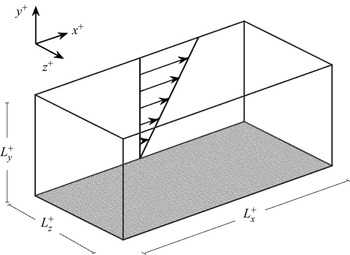
The shear stress-driven flow model of Doohan et al. (Reference Doohan, Willis and Hwang2019, Reference Doohan, Willis and Hwang2021) is considered as a model of wall-bounded turbulence, the flow geometry of which is sketched in figure 1. For full details of the construction and verification of the model, the reader may also refer to Doohan et al. (Reference Doohan, Willis and Hwang2019, Reference Doohan, Willis and Hwang2021). The fully developed turbulent flow in this model defines a time-averaged friction velocity $u_\tau$. Using the friction velocity, this model is re-scaled in inner units, denoted by the superscript $^{+}$, where $t^{+}$ is time, $\boldsymbol {x}^{+}=(x^{+},y^{+},z^{+})$ are the streamwise, wall-normal and spanwise coordinates, $(L_x^{+},L_y^{+},L_z^{+})$ the domain dimensions and $\boldsymbol {u}^{+}=(u^{+},v^{+},w^{+})$ the corresponding velocity components. The wall is located at the lower boundary of the domain denoted by $y^{+}=0$. The velocity field can be expressed in terms of the mean and fluctuating components: $\boldsymbol {u}^{+}(\boldsymbol {x}^{+},t^{+})=\boldsymbol {U}^{+}(y^{+},t^{+})+\boldsymbol {u}'^{+}(\boldsymbol {x}^{+},t^{+})$, where $\boldsymbol {U}^{+}=\langle \boldsymbol {u}^{+} \rangle _{x^{+},z^{+}}$, $\boldsymbol {u}'^{+}=(u'^{+},v'^{+},w'^{+})$ and $\langle {\cdot }\rangle _{x^{+},z^{+}}$ denotes the average in the streamwise and spanwise directions. The time-averaged mean streamwise momentum equation is then given by

(2.1)\begin{equation} \frac{{\rm d}\bar{U}^{+}}{{{\rm d} y}^{+}} - \overline{\langle u'^{+}v'^{+}\rangle}_{x^{+},z^{+}} = 1, \end{equation}

where $\overline {({\cdot })}$ denotes the average in time and $U^{+}$ is the streamwise component of $\boldsymbol {U}^{+}$. We note that (2.1) is approximately valid within the mesolayer for any wall-bounded parallel shear flow in the asymptotic limit $Re_\tau \rightarrow \infty$. For example, in pressure-driven channel flow, an extra term originating from the pressure gradient, $-y^{+}/Re_\tau$, vanishes in this limit, provided that $L_y^{+}$ is within the mesolayer, i.e. $y^{+}\lesssim \sqrt {Re_\tau }$ (e.g. Long & Chen Reference Long and Chen1981; Wei et al. Reference Wei, Fife, Klewicki and McMurtry2005). As $L_y^{+} \rightarrow \infty$, it is not possible to simulate the entirety of the mesolayer as $Re_\tau \rightarrow \infty$. Instead, by choosing a suitable $L_y^{+}$, our simulations resolve the inner-scaling dynamics related to the part of the flow within the mesolayer, i.e. the outer flow is explicitly excluded from the model with an asymptotic scaling, and the part of the inner-scaling flow dynamics, defined by the computational domain, is simulated in isolation like in the minimal flow unit (Jiménez & Moin Reference Jiménez and Moin1991). The choice for $L_y^{+}$ therefore determines the extent of the near-wall region and mesolayer simulated in the asymptotic limit $Re_\tau \rightarrow \infty$, typically informed by observations of near-wall turbulence: for example, in Doohan et al. (Reference Doohan, Willis and Hwang2019), $L_y^{+} \approx 90$ was found to be a reasonable choice with $L_z^{+} \approx 110$ and $L_x^{+} \approx 320$, providing the turbulence statistics and spectra almost identical to those from the minimal-flow-unit simulation in plane Couette flow for $y^{+}\lesssim 50$. In general, the flow statistics resolved in a simulation depend on the value of $L_y^{+}$. However, it remains unchanged below a certain wall-normal location in the flow domain, if $L_y^{+}$ is chosen to be sufficiently large.

Figure 1.

Geometry of the shear stress-driven flow model.

The fluctuating velocity components are governed by the momentum equation

(2.2)\begin{align} \frac{\partial\boldsymbol{u}'^{+}}{\partial t^{+}} +(\boldsymbol{U}^{+}\boldsymbol{\cdot}\boldsymbol{\nabla})\boldsymbol{u}'^{+} +(\boldsymbol{u}'^{+}\boldsymbol{\cdot}\boldsymbol{\nabla})\boldsymbol{U}^{+}&={-}\boldsymbol{\nabla} p'^{+} +\nabla^{2}\boldsymbol{u}'^{+} \nonumber\\ &\quad -\left[(\boldsymbol{u}'^{+}\boldsymbol{\cdot}\boldsymbol{\nabla})\boldsymbol{u}'^{+} -\langle(\boldsymbol{u}'^{+}\boldsymbol{\cdot}\boldsymbol{\nabla})\boldsymbol{u}'^{+}\rangle_{x^{+},z^{+}}\right], \end{align}

where $p'^{+}$ is the pressure fluctuation. The no-slip condition $\boldsymbol {u}^{+}= \boldsymbol {0}$ is imposed at $y^{+}=0$ to represent the stationary wall. At the upper boundary, a horizontally uniform shear stress is applied such that a prescribed bulk flow rate is maintained during the simulation. The imposed boundary condition is identical to that of Doohan et al. (Reference Doohan, Willis and Hwang2021). Periodic boundary conditions are applied in the streamwise and spanwise directions. The numerical simulations in this study were carried out with the diablo Navier–Stokes solver (Bewley Reference Bewley2014). This code employs the Fourier–Galerkin method in the streamwise and spanwise directions with a $2/3$ dealiasing rule, and a second-order finite difference scheme in the wall-normal direction. The temporal discretisation is based on the fractional-step algorithm (Kim & Moin Reference Kim and Moin1985), with implicit treatment of wall-normal derivatives using the Crank–Nicolson scheme and explicit treatment of the remaining terms using a low-storage third-order Runge–Kutta scheme. For further details about the model and its validation, the reader may refer to Doohan et al. (Reference Doohan, Willis and Hwang2019).

In this study, the number of integral length scales is restricted to two as in Doohan et al. (Reference Doohan, Willis and Hwang2021) to consider the simplest multi-scale dynamics of similar order, i.e. near-wall turbulence with two integral length scales of motion. To this end, the domain size is chosen to be $(L_x^{+}=640,L_y^{+}=180,L_z^{+}=220)$ and due to the streamwise- and spanwise-periodic boundary conditions, enforced by expressing the velocity field as a sum of discrete modes according to the Fourier–Galerkin method, the largest velocity structures resolved have spanwise wavenumbers $n=1,2$ and spanwise wavelengths $\lambda _z^{+}\approx 220$ and $\lambda _z^{+}\approx 110$. However, given that the smallest integral length scale is approximately $\lambda _z^{+}\approx 110$ (Jiménez & Moin Reference Jiménez and Moin1991), the remaining smaller velocity structures with higher harmonics would not be viewed to be energy-containing. In this way, the model allows for the analysis of the temporal dynamics of near-wall turbulence sustained at approximately two spanwise integral length scales. Throughout this work, the minimal unit of multi-scale near-wall turbulence is denoted by $\varOmega _2$ and its simulation parameters are summarised in table 1.

Table 1.

Simulation parameters of the minimal unit of multi-scale near-wall turbulence, $\varOmega _2$. Here, $(L_x^{+},L_y^{+},L_z^{+})$ denote the domain dimensions, $N_x$, $N_y$ and $N_z$ the number of grid points in the streamwise, wall-normal and spanwise directions respectively, and $T^{+}$ the duration of the flow simulation.

2.2. Two-scale energy balance

Having introduced the shear stress-driven flow model, the task at hand is to introduce the observables which would well represent the temporal dynamics at two spanwise integral length scales. In this study, we follow the approach in Doohan et al. (Reference Doohan, Willis and Hwang2021), where a binary decomposition of the fluctuating velocity field is first considered in order to separate the energy-containing eddies at each integral length scale, i.e. $\boldsymbol {u}'^{+}=\boldsymbol {u}_l^{+}+\boldsymbol {u}_s^{+}$, where $\boldsymbol {u}_l^{+}=(u_l^{+},v_l^{+},w_l^{+})$ denotes the large-scale velocity field and $\boldsymbol {u}_s^{+}=(u_s^{+},v_s^{+},w_s^{+})$ the small-scale velocity field. Here, $\boldsymbol {u}_l^{+}$ and $\boldsymbol {u}_s^{+}$ are defined as

(2.3a)$$\begin{gather} \boldsymbol{u}_l^{+}=\sum_{|m|\leqslant m_x}\,\sum_{|n|\leqslant 1}\widehat{\boldsymbol{u}_{m,n}'^{+}} \exp({{\rm i}(mk_{x0}^{+}x^{+}+nk_{z0}^{+}z^{+})});\quad |m|+|n|\neq 0, \end{gather}$$

(2.3b)$$\begin{gather}\boldsymbol{u}_s^{+}=\sum_{|m|\leqslant m_x}\,\sum_{2 \leqslant|n|\leqslant n_z}\widehat{\boldsymbol{u}_{m,n}'^{+}} \exp({{\rm i}(mk_{x0}^{+}x^{+}+nk_{z0}^{+}z^{+})}), \end{gather}$$

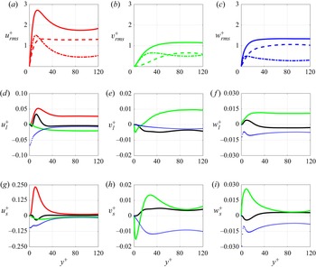
where $\widehat {({\cdot })}$ denotes the Fourier coefficients, $k_{x0}^{+}$ and $k_{z0}^{+}$ are the fundamental streamwise and spanwise wavenumbers, and $m_x$ and $n_z$ are the number of harmonics in the streamwise and spanwise directions. This decomposition is based entirely on the spanwise wavelength and all streamwise wavelengths are included (apart from the spatial mean), because the size of energy-containing eddies in wall-bounded turbulence is well characterised by the spanwise length scale and they are composed of structures of various streamwise length scales (Hwang Reference Hwang2015). The root-mean-squared velocity profiles and their large- and small-scale components are shown in figures 2(a)–2(c). The large-scale structures are relatively uniform across the wall-normal domain (dashed lines) whereas the small-scale structures are much more pronounced near the wall (dash-dotted lines), consistent with Townsend's hypothesis (Townsend Reference Townsend1980). Note that these results (and those in subsequent sections) are plotted over the interval $y^{+}\in [0,120]$ so as to exclude the flow region immediately below the upper boundary.

Figure 2.

Root-mean-squared velocity profiles $(a)$ $u^{+}_{rms}$, $(b)$ $v^{+}_{rms}$ and $(c)$ $w^{+}_{rms}$ (solid lines), decomposed into their large-scale (dashed lines) and small-scale (dash-dotted lines) components. Time-averaged, wall-normal profiles of a selection of terms on the right-hand side of (d)–(f) (2.4) and (g)–(i) (2.5): turbulent production (red), inter-scale turbulent transport (black), pressure strain (green) and dissipation (blue) of $(d)$ $E^{+}_{ul}$ ($P^{+}_{ul},-T^{+}_{\updownarrow,ul},\varPi ^{+}_{ul},\epsilon ^{+}_{ul}$), $(e)$ $E^{+}_{vl}$ ($-T^{+}_{\updownarrow,vl},\varPi ^{+}_{vl},\epsilon ^{+}_{vl}$), $(\,f)$ $E^{+}_{wl}$ ($-T^{+}_{\updownarrow,wl},\varPi ^{+}_{wl},\epsilon ^{+}_{wl}$), $(g)$ $E^{+}_{us}$ ($P^{+}_{us},T^{+}_{\updownarrow,us},\varPi ^{+}_{us},\epsilon ^{+}_{us}$), $(h)$ $E^{+}_{vs}$ ($T^{+}_{\updownarrow,vs},\varPi ^{+}_{vs},\epsilon ^{+}_{vs}$) and $(i)$ $E^{+}_{ws}$ ($T^{+}_{\updownarrow,ws},\varPi ^{+}_{ws},\epsilon ^{+}_{ws}$).

Substitution of $\boldsymbol {u}_l^{+}$ and $\boldsymbol {u}_s^{+}$ into (2.2) yields the large- and small-scale momentum equations

(2.4)\begin{equation} \left.\begin{gathered} \frac{\partial \boldsymbol{u}^{+}_l}{\partial t^{+}} +(\boldsymbol{U}^{+}\boldsymbol{\cdot}\boldsymbol{\nabla})\boldsymbol{u}^{+}_l={-}(\boldsymbol{u}^{+}_l\boldsymbol{\cdot}\boldsymbol{\nabla})\boldsymbol{U}^{+} -\boldsymbol{\nabla} p^{+}_l +\nabla^{2}\boldsymbol{u}^{+}_l \\ -\mathcal{P}_l\{(\boldsymbol{u}^{+}_l\boldsymbol{\cdot}\boldsymbol{\nabla})\boldsymbol{u}^{+}_l +(\boldsymbol{u}^{+}_l\boldsymbol{\cdot}\boldsymbol{\nabla})\boldsymbol{u}^{+}_s +(\boldsymbol{u}^{+}_s\boldsymbol{\cdot}\boldsymbol{\nabla})\boldsymbol{u}^{+}_l +(\boldsymbol{u}^{+}_s\boldsymbol{\cdot}\boldsymbol{\nabla})\boldsymbol{u}^{+}_s\} \end{gathered}\right\} \end{equation}

and

(2.5)\begin{equation} \left.\begin{gathered} \frac{\partial \boldsymbol{u}^{+}_s}{\partial t^{+}} +(\boldsymbol{U}^{+}\boldsymbol{\cdot}\boldsymbol{\nabla})\boldsymbol{u}^{+}_s={-}(\boldsymbol{u}^{+}_s\boldsymbol{\cdot}\boldsymbol{\nabla})\boldsymbol{U}^{+} -\boldsymbol{\nabla} p^{+}_s +\nabla^{2}\boldsymbol{u}^{+}_s \\ -\mathcal{P}_s\{ (\boldsymbol{u}^{+}_s\boldsymbol{\cdot}\boldsymbol{\nabla})\boldsymbol{u}^{+}_s +(\boldsymbol{u}^{+}_s\boldsymbol{\cdot}\boldsymbol{\nabla})\boldsymbol{u}^{+}_l +(\boldsymbol{u}^{+}_l\boldsymbol{\cdot}\boldsymbol{\nabla})\boldsymbol{u}^{+}_s +(\boldsymbol{u}^{+}_l\boldsymbol{\cdot}\boldsymbol{\nabla})\boldsymbol{u}^{+}_l\}, \end{gathered}\right\} \end{equation}

where $p'^{+}=p_l^{+}+p_s^{+}$ are the large- and small-scale pressure fluctuations that enforce continuity of the large- and small-scale velocity fields, and $\mathcal {P}_l\{{\cdot }\}$ and $\mathcal {P}_s\{{\cdot }\}$ denote projection onto large and small scales, respectively. Using (2.4) and (2.5), the componentwise energy-balance equations at each scale can be defined, as detailed in Doohan et al. (Reference Doohan, Willis and Hwang2021). Multiplying (2.4) by $\boldsymbol {u}_l^{+}$ and averaging in the streamwise and spanwise directions with some further rearrangement of nonlinear terms, the large-scale energy balance equation is written as

(2.6a)$$\begin{gather} \frac{\partial E^{+}_{ul}}{\partial t^{+}}= P^{+}_{ul}-T^{+}_{u,\updownarrow}+T^{+}_{ul,-}+T^{+}_{ul,\#}+\varPi^{+}_{ul}+T^{+}_{\nu,ul}+\epsilon^{+}_{ul}, \end{gather}$$

(2.6b)$$\begin{gather}\frac{\partial E^{+}_{vl}}{\partial t^{+}}= T^{+}_{p,vl}-T^{+}_{v,\updownarrow}+T^{+}_{vl,-}+T^{+}_{vl,\#} +\varPi^{+}_{vl}+T^{+}_{\nu,vl}+\epsilon^{+}_{vl}, \end{gather}$$

(2.6c)$$\begin{gather}\frac{\partial E^{+}_{wl}}{\partial t^{+}}={-}T^{+}_{w,\updownarrow}+T^{+}_{wl,-}+T^{+}_{wl,\#} +\varPi^{+}_{wl}+T^{+}_{\nu,wl}+\epsilon^{+}_{wl}, \end{gather}$$

where

(2.7a–c)\begin{equation} E^{+}_{ul}=\tfrac{1}{2}\langle (u_l^{+})^{2} \rangle_{x^{+},z^{+}}, \quad E^{+}_{vl}=\tfrac{1}{2}\langle (v_l^{+})^{2} \rangle_{x^{+},z^{+}} \quad \mathrm{and} \quad E^{+}_{wl}=\tfrac{1}{2}\langle (w_l^{+})^{2} \rangle_{x^{+},z^{+}} \end{equation}

are large-scale streamwise, wall-normal and spanwise kinetic energy, $P^{+}_{ul}$ is large-scale turbulent production, 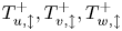$T^{+}_{u,\updownarrow }, T^{+}_{v,\updownarrow }, T^{+}_{w,\updownarrow }$ are streamwise, wall-normal and spanwise ‘inter-scale’ turbulent transport, $T^{+}_{ul,-}, T^{+}_{vl,-}, T^{+}_{wl,-}$ large-scale streamwise, wall-normal and spanwise ‘intra-scale spatial’ turbulent transport, $T^{+}_{ul,\#}, T^{+}_{vl,\#}, T^{+}_{wl,\#}$ large-scale streamwise, wall-normal and spanwise ‘inter-scale spatial’ turbulent transport, $\varPi ^{+}_{ul}$, $\varPi ^{+}_{vl}$ and $\varPi ^{+}_{wl}$ large-scale streamwise, wall-normal and spanwise pressure strain, $T^{+}_{p,vl}$ is large-scale pressure transport, $T^{+}_{\nu,ul}$, $T^{+}_{\nu,vl}$ and $T^{+}_{\nu,wl}$ are large-scale streamwise, wall-normal and spanwise viscous transport, and $\epsilon ^{+}_{ul}$, $\epsilon ^{+}_{vl}$ and $\epsilon ^{+}_{wl}$ are large-scale streamwise, wall-normal and spanwise dissipation. Similarly, using (2.5) the small-scale energy balance equation is obtained as

(2.8a)$$\begin{gather} \frac{\partial E^{+}_{us}}{\partial t^{+}}= P^{+}_{us}+T^{+}_{u,\updownarrow}+T^{+}_{us,-}+T^{+}_{us,\#} +\varPi^{+}_{us}+T^{+}_{\nu,us}+\epsilon^{+}_{us}, \end{gather}$$

(2.8b)$$\begin{gather}\frac{\partial E^{+}_{vs}}{\partial t^{+}}= T^{+}_{p,vs}+T^{+}_{v,\updownarrow}+T^{+}_{vs,-}+T^{+}_{vs,\#} +\varPi^{+}_{vs}+T^{+}_{\nu,vs}+\epsilon^{+}_{vs}, \end{gather}$$

(2.8c)$$\begin{gather}\frac{\partial E^{+}_{ws}}{\partial t^{+}}= T^{+}_{w,\updownarrow}+T^{+}_{ws,-}+T^{+}_{ws,\#} +\varPi^{+}_{ws}+T^{+}_{\nu,ws}+\epsilon^{+}_{ws}, \end{gather}$$

in which

(2.9a–c)\begin{equation} E^{+}_{us}=\tfrac{1}{2}\langle (u_s^{+})^{2} \rangle_{x^{+},z^{+}}, \quad E^{+}_{vs}=\tfrac{1}{2}\langle (v_s^{+})^{2} \rangle_{x^{+},z^{+}} \quad \mathrm{and} \quad E^{+}_{ws}=\tfrac{1}{2}\langle (w_s^{+})^{2} \rangle_{x^{+},z^{+}} \end{equation}

are small-scale streamwise, wall-normal and spanwise kinetic energy, $P^{+}_{us}$ is small-scale turbulent production, $T^{+}_{us,-}, T^{+}_{vs,-}, T^{+}_{ws,-}$ are small-scale streamwise, wall-normal and spanwise ‘intra-scale spatial’ turbulent transport, $T^{+}_{us,\#}, T^{+}_{vs,\#}, T^{+}_{ws,\#}$ small-scale streamwise, wall-normal and spanwise ‘inter-scale spatial’ turbulent transport, $\varPi ^{+}_{us}$, $\varPi ^{+}_{vs}$ and $\varPi ^{+}_{ws}$ are small-scale streamwise, wall-normal and spanwise pressure strain, $T^{+}_{p,vs}$ is small-scale pressure transport, $T^{+}_{\nu,us}$, $T^{+}_{\nu,vs}$ and $T^{+}_{\nu,ws}$ small-scale streamwise, wall-normal and spanwise viscous transport, and $\epsilon ^{+}_{us}$, $\epsilon ^{+}_{vs}$ and $\epsilon ^{+}_{ws}$ small-scale streamwise, wall-normal and spanwise dissipation. The definitions of the terms in the large- and small-scale energy balance equations are given in full in supplementary material § 1 available at https://doi.org/10.1017/jfm.2022.686.

Some key features of the terms defined in (2.6) and (2.8) are subsequently discussed. The turbulent production terms $P^{+}_{ul}$ and $P^{+}_{us}$ originate from the first linear term in the right-hand side of (2.4) and (2.5), and they represent the linear mechanisms through which the large- and small-scale velocity fluctuations extract energy from the mean velocity. If averaged in time and the wall-normal direction, the production terms are perfectly balanced with the dissipation terms:

(2.10)\begin{equation} \overline{\langle P^{+}_{ul}+P^{+}_{us} \rangle_{y^{+}}}=\overline{\langle \epsilon^{+}_{ul}+\epsilon^{+}_{vl}+\epsilon^{+}_{wl}+\epsilon^{+}_{us}+\epsilon^{+}_{vs}+\epsilon^{+}_{ws} \rangle_{y^{+}}}. \end{equation}

The pressure strain and transport terms involve both linear and nonlinear mechanisms, because the pressure is driven by ‘fast’ linear and ‘slow’ nonlinear terms in (2.6) and (2.8) (Kim Reference Kim1989). From the continuity equation, the pressure strain terms at each scale also satisfy $-\varPi ^{+}_{ul}=\varPi ^{+}_{vl}+\varPi ^{+}_{wl}$ and $-\varPi ^{+}_{us}=\varPi ^{+}_{vs}+\varPi ^{+}_{ws}$, playing a crucial role in the distribution of TKE produced in the streamwise component to the wall-normal and spanwise components (Cho et al. Reference Cho, Hwang and Choi2018). In particular, at the integral length scale, this process was found to be closely associated with the streak instability/breakdown in the SSP at each scale (Doohan et al. Reference Doohan, Willis and Hwang2021). Turbulent transport, which originates from the nonlinear terms in (2.4) and (2.5), is broken down into ‘inter-scale’ transport (with subscript ‘$_\updownarrow$’), ‘inter-scale spatial’ transport (with subscript ‘$_\#$’) and ‘intra-scale spatial’ transport (with subscript ‘$_-$’). The inter-scale transport terms,

(2.11a)$$\begin{gather} T^{+}_{u,\updownarrow}=\langle u_l^{+}(\boldsymbol{u}^{+}_l\boldsymbol{\cdot}\boldsymbol{\nabla} u_s^{+})\rangle_{x^{+},z^{+}} - \langle u_s^{+}(\boldsymbol{u}^{+}_s\boldsymbol{\cdot}\boldsymbol{\nabla} u_l^{+}) \rangle_{x^{+},z^{+}}, \end{gather}$$

(2.11b)$$\begin{gather}T^{+}_{v,\updownarrow}=\langle v_l^{+}(\boldsymbol{u}^{+}_l\boldsymbol{\cdot}\boldsymbol{\nabla} v_s^{+})\rangle_{x^{+},z^{+}} - \langle v_s^{+}(\boldsymbol{u}^{+}_s\boldsymbol{\cdot}\boldsymbol{\nabla} v_l^{+}) \rangle_{x^{+},z^{+}}, \end{gather}$$

(2.11c)$$\begin{gather}T^{+}_{w,\updownarrow}=\langle w_l^{+}(\boldsymbol{u}^{+}_l\boldsymbol{\cdot}\boldsymbol{\nabla} w_s^{+})\rangle_{x^{+},z^{+}} - \langle w_s^{+}(\boldsymbol{u}^{+}_s\boldsymbol{\cdot}\boldsymbol{\nabla} w_l^{+}) \rangle_{x^{+},z^{+}}, \end{gather}$$

depend on both large- and small-scale velocity components and are shared by (2.6) and (2.8) with opposite sign, indicating that they play a role in the direct same-component exchange of TKE between different scales. The ‘inter-scale spatial’ transport terms also represent a type of scale interaction and depend on both large- and small-scale velocity components. However, the resulting energy transfer only takes place locally in space (i.e. in the wall-normal direction), because there is no ‘net’ transfer generated from

(2.12)\begin{equation} \left.\begin{gathered} \langle T^{+}_{ul,\#} \rangle_{y^{+}}=\langle T^{+}_{vl,\#} \rangle_{y^{+}}=\langle T^{+}_{wl,\#} \rangle_{y^{+}}=0, \\ \langle T^{+}_{us,\#} \rangle_{y^{+}}=\langle T^{+}_{vs,\#} \rangle_{y^{+}}=\langle T^{+}_{ws,\#} \rangle_{y^{+}}=0, \end{gathered}\right\} \end{equation}

as per their definitions (see supplementary material § 1). Finally, the ‘intra-scale spatial’ transport terms are only associated with the redistribution of energy across space induced by velocity components of the same scale. Given the nature of the turbulent transport terms discussed here, the primary focus in this study will be given to studying the inter-scale direct turbulent transport in (2.11). The statistics of the production, inter-scale turbulent transport, pressure strain and dissipation terms discussed previously are shown in figure 2. For further discussion of these variables, the reader may refer to Doohan et al. (Reference Doohan, Willis and Hwang2021), in which their statistical characteristics, temporal dynamics and cross-correlations are extensively studied. Note that the statistical profiles of the intra- and inter-scale spatial turbulent transport terms are plotted in figure 4 of that work.

2.3. Observables

Time-dependent observables, required for the construction of phase portraits, are now defined by suitably averaging the terms in (2.6) and (2.8) in the wall-normal direction. Here, it should be mentioned that the decomposition (2.3) for the energy-balance equations (2.6) and (2.8) is only introduced as a matter of convenience. Indeed, the energy transfer dynamics have been found to vary considerably across the wall-normal domain. For instance, $E_{us}^{+}$ in (2.8) not only contains the energy of the small-scale anisotropic near-wall coherent structures (e.g. streaks) but also that of relatively isotropic small-scale eddies generated by the energy cascade from the large-scale structures. Given the two completely different origins of the dynamics involved in $E_{us}^{+}$ depending on the wall-normal location, the limits of integration in $y^{+}$ have been chosen carefully as discussed in detail in Doohan et al. (Reference Doohan, Willis and Hwang2021). In subsequent sections, the same notation is used to denote the $y^{+}$-averaged terms but the corresponding limits of integration are also indicated for the time-dependent observables: for example, $T^{+}_{u,\updownarrow }|_{45}^{120}$ is the streamwise inter-scale turbulent transport term averaged over the interval $y^{+}\in [45,120]$.

While the observables defined with the terms in (2.6) and (2.8) are useful to understand the energy transfer dynamics between large and small scales, they are not very informative about the dynamics of the coherent structures within each scale. The dynamics of the structures at each scale has been well understood in terms of the SSP which involves the interplay between rolls, streaks and the streak-instability waves (e.g. Hamilton et al. Reference Hamilton, Kim and Waleffe1995; Hwang & Bengana Reference Hwang and Bengana2016). Therefore, the observables representing these fundamental structural elements are also defined by further decomposing the velocity components into their streamwise-independent and streamwise-dependent parts. The kinetic energies of large-scale straight streaks (ss), wavy streaks (ws), straight rolls (sr) and wavy rolls (wr) are defined as

(2.13a)$$\begin{gather} E^{+}_{ss,l}(t^{+})=\left.\tfrac{1}{2}\langle \langle u_l^{+} \rangle_{x^{+}}^{2} \rangle_{z^{+}}\right|_{0}^{120}, \end{gather}$$

(2.13b)$$\begin{gather}E^{+}_{ws,l}(t^{+})=\left.\tfrac{1}{2}\langle (u_l^{+}- \langle u_l^{+} \rangle_{x^{+}})^{2} \rangle_{x^{+},z^{+}}\right|_{0}^{120}, \end{gather}$$

(2.13c)$$\begin{gather}E^{+}_{sr,l}(t^{+})=\left.\tfrac{1}{2}\langle \langle v_l^{+} \rangle_{x^{+}}^{2} + \langle w_l^{+} \rangle_{x^{+}}^{2} \rangle_{z^{+}}\right|_{0}^{120}, \end{gather}$$

(2.13d)$$\begin{gather}E^{+}_{wr,l}(t^{+})=\left.\tfrac{1}{2}\langle (v_l^{+}- \langle v_l^{+} \rangle_{x^{+}})^{2} + (w_l^{+}- \langle w_l^{+} \rangle_{x^{+}})^{2} \rangle_{x^{+},z^{+}}\right|_{0}^{120}, \end{gather}$$

respectively, while the kinetic energies of small-scale straight streaks, wavy streaks, straight rolls and wavy rolls are defined as

(2.14a)$$\begin{gather} E^{+}_{ss,s}(t^{+})=\left.\tfrac{1}{2}\langle \langle u_s^{+} \rangle_{x^{+}}^{2} \rangle_{z^{+}}\right|_{0}^{45}, \end{gather}$$

(2.14b)$$\begin{gather}E^{+}_{ws,s}(t^{+})=\left.\tfrac{1}{2}\langle (u_s^{+}- \langle u_s^{+} \rangle_{x^{+}})^{2} \rangle_{x^{+},z^{+}}\right|_{0}^{45}, \end{gather}$$

(2.14c)$$\begin{gather}E^{+}_{sr,s}(t^{+})=\left.\tfrac{1}{2}\langle \langle v_s^{+} \rangle_{x^{+}}^{2} + \langle w_s^{+} \rangle_{x^{+}}^{2} \rangle_{z^{+}}\right|_{0}^{45}, \end{gather}$$

(2.14d)$$\begin{gather}E^{+}_{wr,s}(t^{+})=\left.\tfrac{1}{2}\langle (v_s^{+}- \langle v_s^{+} \rangle_{x^{+}})^{2} + (w_s^{+}- \langle w_s^{+} \rangle_{x^{+}})^{2} \rangle_{x^{+},z^{+}}\right|_{0}^{45}, \end{gather}$$

respectively. Finally, it has been found that there exists an inverse energy transfer from small to large scales in the region close to the wall (Cho et al. Reference Cho, Hwang and Choi2018), which has been referred to as ‘feeding’ (Doohan et al. Reference Doohan, Willis and Hwang2021). The structures that emerge from the feeding process are primarily localised streamwise and spanwise velocity fluctuations, and they are ‘inactive’ in the sense that they carry little to no Reynolds shear stress (Townsend Reference Townsend1980). Following Doohan et al. (Reference Doohan, Willis and Hwang2021), the large-scale inactive structures resulting from the streamwise feeding process are measured through the near-wall kinetic energy of wavy streamwise motion

(2.15)\begin{equation} E^{+}_{wu,i}=\left.\tfrac{1}{2}\langle(u_l^{+}- \langle u_l^{+} \rangle_{x^{+}})^{2} \rangle_{x^{+},z^{+}}\right|_{0}^{20}. \end{equation}

3.1. Computation of solutions

Doohan et al. (Reference Doohan, Willis and Hwang2019) computed invariant solutions for a single-scale minimal unit using the Newton–Krylov–Hooksetp algorithm (Viswanath Reference Viswanath2007, Reference Viswanath2009; Gibson et al. Reference Gibson, Halcrow and Cvitanovic2008; Willis et al. Reference Willis, Cvitanović and Avila2013). Given a velocity field $\boldsymbol {u}^{+}$ that is expected to be close to an invariant solution, this method minimises the relative error

(3.1)\begin{equation} r=\frac{||\sigma({-}s_x^{+},-s_z^{+})\,{\boldsymbol{\varPhi}}^{T^{+}} (\boldsymbol{u}^{+})-\boldsymbol{u}^{+}||}{||\boldsymbol{u}^{+}||}, \end{equation}

where $\boldsymbol {\varPhi }^{T^{+}}$ is the Navier–Stokes propagator, which integrates $\boldsymbol {u}^{+}$ forward in time by a period $T^{+}$, and $\sigma$ applies a spatial shift to the resulting velocity field by distances $-s_x$ and $-s_z$. The minus sign indicates that these shifts are in the negative $x$ and $z$ direction, in particular to counter the downstream advection of the solutions. The phase speeds of the solution are $c_x^{+}=s_x^{+}/T^{+}$, $c_z^{+}=s_z^{+}/T^{+}$, being careful to ensure that the shifts have not been aliased by a period of the domain. For periodic orbits, $T^{+}$ also needs to be determined, while for travelling waves the choice of $T^{+}$ is arbitrary, usually taken to be of order $10$. The domain $\varOmega _1$ in which the solutions were calculated by Doohan et al. (Reference Doohan, Willis and Hwang2019) had dimensions $L_x^{+}=320$, $L_y^{+}=90$ and $L_z^{+}=110$, i.e. each dimension is half that of the domain $\varOmega _2$ of the present study, given in table 1. Although this is quite a difference in domain size, it is expected that it should be possible to use the same Newton-based algorithm to numerically continue at least a subset of the invariant solutions to $\varOmega _2$.

During the continuation, the aspect ratio of the flow domain $L_x^{+}:L_y^{+}:L_z^{+}$ is held fixed, and the shift-reflect symmetry

(3.2)\begin{equation} [u^{+},v^{+},w^{+}](x^{+},y^{+},z^{+}) = [u^{+},v^{+},-w^{+}](x^{+}+L_x^{+}/2,y^{+},-z^{+}) \end{equation}

is preserved. It is also possible to numerically continue the invariant solutions by increasing the wall-normal domain height from $L_y^{+}=90$ to $L_y^{+}=180$ while maintaining $L_x^{+}=320$ and $L_z^{+}=110$ fixed. These solutions can then be concatenated in the streamwise and spanwise directions, forming a solution with four copies of the structure in the larger two-scale domain $\varOmega _2$. These solutions satisfy the periodic boundary conditions of $\varOmega _2$, so that the concatenated velocity field is an exact solution in $\varOmega _2$ with the same phase speeds $c_x^{+}$ and $c_z^{+}$, and time period $T^{+}$. Solutions constructed in this manner exhibit the half-shift-reflect symmetry

(3.3)\begin{equation} [u^{+},v^{+},w^{+}](x^{+},y^{+},z^{+}) = [u^{+},v^{+},-w^{+}](x^{+}+L_x^{+}/4,y^{+},-z^{+}), \end{equation}

where here $L_x^{+}=640$ is the streamwise dimension of $\varOmega _2$. A critical limitation of the latter continuation approach is that these structures, due to their streamwise and spanwise periodicity within the flow domain, do not include the fundamental streamwise and spanwise wavenumbers, nor indeed all wavenumbers associated with odd $m$ and $n$ in (2.3). Clearly, the solutions computed in this manner do not capture the large-scale structures with spanwise wavelength $\lambda _z^{+}=220$ in (2.3a). Therefore, the invariant solutions obtained using the concatenation approach will be called the small-scale solutions, whereas those obtained through fixed-aspect ratio numerical continuation will be called the large-scale solutions.

Likewise, it is acknowledged that the continuation approach is also not ideal, in the sense that there is no explicit introduction of activity at multiple length scales. There is no robust approach, however, to finding or constructing such solutions. The search for recurrences, or quiescent periods, in the turbulent dynamics has been fruitful in identifying solutions in minimal domains, but the substantial extra degrees of freedom of the two-scale domain imply that the probability of experiencing a sufficiently close recurrence is vanishingly small. We have experimented with the superposition of some large- and small-scale solutions in order to construct a two-scale solution without success. Solutions that inherently include multi-scale activity might also be more naturally represented by a relative periodic orbit. However, as the period natural to the self-sustaining cycle at each scale is unlikely to be the same, this implies that periods for the overall multi-scale orbit may be infinite (quasi-periodic) or too long to be captured at present.

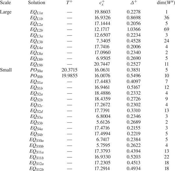
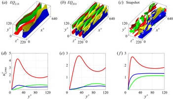
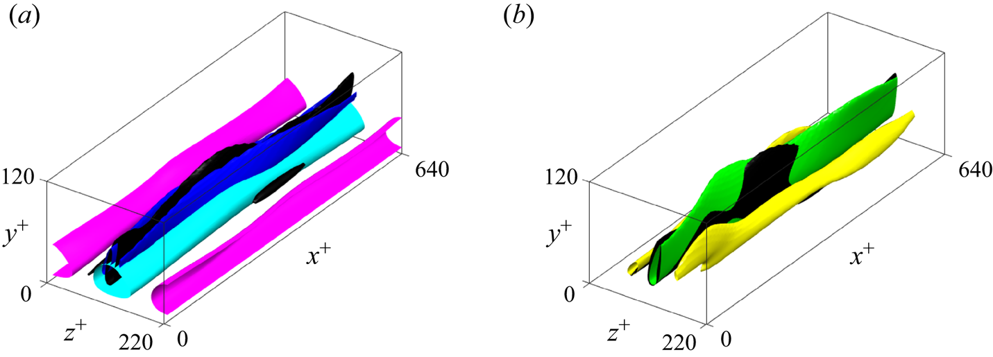
Using the continuation and concatenation approaches, in total, 10 large-scale solutions and 18 small-scale solutions have been computed in the minimal unit of multi-scale near-wall turbulence $\varOmega _2$. The relative error $r$ of all solutions reported in this work is less than $10^{-6}$. Their properties are summarised in table 2. A representative large-scale solution ($EQ_{L1b}$) and small-scale solution ($EQ_{S1b}$) are plotted in figure 3, together with a turbulent snapshot for reference. A detailed description of each of the large- and small-scale solutions is given in supplementary material § 2.

Table 2.

Properties of the large- and small-scale invariant solutions in the minimal unit of multi-scale near-wall turbulence $\varOmega _2$: the time period $T^{+}$, the phase speed $c_x^{+}$, the wall shear rate $\varDelta ^{+}$ and the dimension of the unstable manifold within the corresponding subspace $\textrm {dim}(W^{u})$. The values of $c_x^{+}$ and $\varDelta ^{+}$ of $PO_{S0a}$ and $PO_{S0b}$ are averages over the corresponding time period $T^{+}$.

Figure 3.

Velocity field visualisation and root mean squared velocity profiles of two invariant solutions and the turbulent state. High- and low-speed streaks $u'^{+}$ are shown in red/blue, and positive and negative wall-normal velocity isosurfaces $v'^{+}$ are shown in yellow/green respectively: (a,d) $EQ_{L1b}$, $u'^{+}=\pm 3.50$, $v'^{+}=\pm 0.90$; (b,e) $EQ_{S1b}$, $u'^{+}=\pm 2.20$, $v'^{+}=\pm 0.50$; (c,f) a turbulent snapshot, $u'^{+}=\pm 3.50$, $v'^{+}=\pm 2.00$. The $u^{+}_{rms}$, $v^{+}_{rms}$ and $w^{+}_{rms}$ profiles are shown in red, green and blue, respectively.

3.2. Bifurcation of solutions

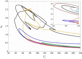
As described previously, the large-scale solutions are obtained through fixed-aspect ratio numerical continuation from the minimal unit $\varOmega _1$ to the minimal unit of multi-scale near-wall turbulence $\varOmega _2$. However, it is also of interest to analyse the bifurcation of both large- and small-scale solutions over the domain size in order to establish connections between the solutions. The invariant solutions are continued over a range of values of the spanwise domain width $L_z^{+}$ whereas maintaining the aspect ratio of the flow domain fixed. The numerical continuation is carried out using a pseudo-arclength continuation algorithm and the resulting $(L_z^{+},\varDelta ^{+})$ bifurcation diagram is plotted in figure 4, where $\varDelta ^{+}$ is the time-averaged wall shear rate:

(3.4)\begin{equation} \varDelta^{+}=\left.\frac{{\rm d}\bar{U}^{+}}{{{\rm d}y}^{+}}\right\vert_{y^{+}=0} .\end{equation}

We note that the time-averaged wall shear rate of turbulent state is unity (i.e. $\varDelta ^{+}=1$; see (2.1)).

Figure 4.

The $(L_z^{+},\varDelta ^{+})$ bifurcation diagram of the large-scale invariant solutions: black line, $EQ_{L1a}$ and $EQ_{L1b}$; gold line, $EQ_{L2a}$ and $EQ_{L2b}$; dark blue line, $EQ_{L3a}$ and $EQ_{L3b}$; red line, $EQ_{L4a}$; dark green line, $EQ_{L8a}$ and $EQ_{L8b}$. The insert shows the $(L_z^{+},\varDelta ^{+})$ bifurcation diagram of the small-scale invariant solutions: brown line, $PO_{S0a}$ and $PO_{S0b}$; black line, $EQ_{S1a}$ and $EQ_{S1b}$; gold line, $EQ_{S2a}$ and $EQ_{S2b}$; orange line, $EQ_{S2c}$ and $EQ_{S2d}$; dark blue line, $EQ_{S3a}$ and $EQ_{S3b}$; red line, $EQ_{S4a}$ and $EQ_{S4b}$; purple line, $EQ_{S10a}$ and $EQ_{S10b}$; grey line, $EQ_{S11a}$ and $EQ_{S11b}$; light blue line, $EQ_{S12a}$ and $EQ_{S12b}$. The $\varDelta ^{+}$ values of $PO_{S0a}$ and $PO_{S0b}$ are averages over the corresponding time period $T^{+}$.

The large-scale solutions $EQ_{L1a}$ and $EQ_{L1b}$ emerge in a saddle-node bifurcation at $L_z^{+}\approx 35$ (black line). A secondary solution curve emerges at $L_z^{+}\approx 77$ on the upper branch, which exhibits highly erratic behaviour at low values of $L_z^{+}$ before rejoining the primary solution curve at the same point. The solutions $EQ_{L2a}$ and $EQ_{L2b}$ appear in a saddle-node bifurcation at $L_z^{+}\approx 60$ (gold line). The upper branch is highly complex at $L_z^{+}\approx 80$, but it varies smoothly with $L_z^{+}$ above $L_z^{+}\approx 90$, along which the solution $EQ_{L2b}$ was obtained. The solutions $EQ_{L3a}$ and $EQ_{L3b}$ (dark blue line), $EQ_{L4a}$ (red line) and $EQ_{L8a}$ and $EQ_{L8b}$ (dark green line) also emerge in saddle-node bifurcations at $L_z^{+}\approx 47$, $L_z^{+}\approx 67$ and $L_z^{+}\approx 112$, respectively. The upper branch of $EQ_{L4a}$ could not be traced up to $L_z^{+}=220$, because the relative error began to increase above the desired threshold. Furthermore, $EQ_{L9b}$ was not amenable to fixed-aspect ratio numerical continuation and so it does not appear in figure 4.

The $(L_z^{+},\varDelta ^{+})$ bifurcation diagram of the small-scale solutions is plotted in the insert in figure 4, all of which also emerge in saddle-node bifurcations. However, the bifurcation points occur at much higher values of $L_z^{+}$, ranging from $L_z^{+}\approx 180$ for $PO_{S0a}$ and $PO_{S0b}$ (brown line) to $L_z^{+}\approx 217$ for $EQ_{S2a}$ and $EQ_{S2b}$ (gold line). It should be recalled that the small-scale solutions are obtained through velocity field concatenation and so they capture two sets of small-scale structures with spanwise wavelengths $\lambda _z^{+}=110$, as defined in (2.3). Therefore, this range of values of the bifurcation points is consistent with twice the characteristic spacing of near-wall streaks (e.g. Kline et al. Reference Kline, Reynolds, Schraub and Runstadler1967). The proximity of $\varOmega _2$ to the bifurcation points of the small-scale solutions would also explain the lack of velocity field diversity in supplementary material § 2.2, because there would be little difference between lower- and upper-branch solutions close to the bifurcation point and more diverse solutions may emerge at higher values of $L_z^{+}$. Finally, it is evident that the values of the wall shear rate $\varDelta ^{+}$ of most of the large- and small-scale solutions in $\varOmega _2$ (i.e. $L_z^{+}=220$ in figure 4) are considerably lower than that of the corresponding turbulent state ($\varDelta ^{+}=1$). Only $EQ_{L1b}$ and $EQ_{L2b}$ attain values comparable to that of the mean turbulent state (see table 2).

3.3. Phase portraits

The visualisation of the state space using suitably defined phase portraits is a key concept in the dynamical systems framework, which helps to rationalise the chaotic dynamics in terms of the geometrical structure of trajectories in the state space. While equilibria correspond to points in the state space, their stable and unstable manifolds characterise the local state space dynamics. In low-dimensional dynamical systems, the hope was that a sufficiently large number of such invariant solutions (including periodic orbits) would be able to offer physical insight into the global state-space dynamics of turbulence (Kerswell Reference Kerswell2005; Eckhardt et al. Reference Eckhardt, Schneider, Hof and Westerweel2007; Kawahara et al. Reference Kawahara, Uhlmann and Van Veen2012; Graham & Floryan Reference Graham and Floryan2020). Indeed, this approach has been successful in the characterisation of transition to turbulence in wall-bounded shear flows (e.g. Gibson et al. Reference Gibson, Halcrow and Cvitanovic2008; Kreilos & Eckhardt Reference Kreilos and Eckhardt2012; Zammert & Eckhardt Reference Zammert and Eckhardt2015), especially when the computational domain of interest is sufficiently small to avoid the further complexity of spatiotemporal effects (for the spatiotemporal nature of transition, see the review by Barkley Reference Barkley2016). Furthermore, for a turbulent flow at sufficiently low Reynolds numbers, in which the dynamics are dominated by the SSP at a single integral length scale (Jiménez & Moin Reference Jiménez and Moin1991; Hamilton et al. Reference Hamilton, Kim and Waleffe1995; Doohan et al. Reference Doohan, Willis and Hwang2019), it has been observed that the upper-branch solutions typically resemble the turbulent state (e.g. Gibson et al. Reference Gibson, Halcrow and Cvitanovic2009; Willis et al. Reference Willis, Cvitanović and Avila2013; Doohan et al. Reference Doohan, Willis and Hwang2019), whereas a few of the lower-branch solutions constitute the edge state (e.g. Itano & Toh Reference Itano and Toh2001; Skufca et al. Reference Skufca, Yorke and Eckhardt2006; Schneider et al. Reference Schneider, Eckhardt and Yorke2007, Reference Schneider, Gibson, Lagha, De Lillo and Eckhardt2008).

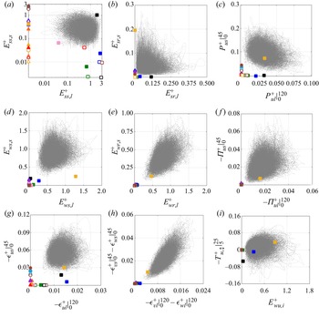
Having computed a number of solutions in $\varOmega _2$ and analysed their bifurcation behaviour, the ability of the invariant solutions to capture the dynamics of near-wall turbulence with two integral length scales of motion is now assessed. Recalling the large-scale kinetic energy terms in (2.13), the small-scale kinetic energy terms in (2.14) and the terms in the large- and small-scale energy balance equations in (2.6) and (2.8), the turbulent trajectory and the large- and small-scale solutions are plotted in various phase portraits in figure 5.

Figure 5.

Phase portraits of the turbulent trajectory (dotted grey line) and the invariant solutions in the following planes: $(a)$ $(E^{+}_{ss,l},E^{+}_{ss,s})$; $(b)$ $(E^{+}_{sr,l},E^{+}_{sr,s})$; $(c)$ $(P^{+}_{ul}|_{0}^{120},P^{+}_{us}|_{0}^{45})$; $(d)$ $(E^{+}_{ws,l},E^{+}_{ws,s})$; $(e)$ $(E^{+}_{wr,l},E^{+}_{wr,s})$; $(\,f)$ $(-\varPi ^{+}_{ul}|_{0}^{120},-\varPi ^{+}_{us}|_{0}^{45})$; $(g)$ $(-\epsilon ^{+}_{ul}|_{0}^{120},-\epsilon ^{+}_{us}|_{0}^{45})$; $(h)$ $(-\epsilon ^{+}_{vl}|_{0}^{120}-\epsilon ^{+}_{wl}|_{0}^{120},-\epsilon ^{+}_{vs}|_{0}^{45}-\epsilon ^{+}_{ws}|_{0}^{45})$; $(i)$ $(E^{+}_{wu,i},-T^{+}_{u,\updownarrow }|_{5}^{25})$. The edge state and the large-scale equilibrium solutions are plotted as squares, the small-scale equilibrium solutions as triangles and the small-scale periodic orbits as circles. The colour scheme is identical to that in figure 4, with the addition of the edge state in brown and $EQ_{L9b}$ in pink. Lower-branch solutions have unfilled symbols and upper-branch solutions have filled symbols. The values for the edge state, $PO_{S0a}$ and $PO_{S0b}$ are averages over the corresponding time period $T^{+}$.

The $(E^{+}_{ss,l},E^{+}_{ss,s})$ phase portrait is shown in figure 5$(a)$. As expected, the small-scale equilibrium solutions (triangles) and small-scale periodic orbits (circles) do not capture any large-scale structures and lie along the ordinate, exhibiting a wide range of values of $E^{+}_{ss,s}$. Indeed, this is observed in all of the remaining phase portraits in figures 5(b)–5(i). The large-scale solutions (squares) exhibit significant values of $E^{+}_{ss,l}$, some of which are close to the maximum values attained by the turbulent trajectory, consistent with the strong straight streaks identified in the velocity field visualisations in supplementary material figure 2. However, most of the large-scale solutions do not feature typical values of $E^{+}_{ss,s}$ and are positioned well below the turbulent trajectory in figure 5$(a)$. This indicates that there is little development of small-scale structures during the numerical continuation of invariant solutions from $\varOmega _1$ to $\varOmega _2$, at least in most cases. Only $EQ_{L1b}$ (filled black square) exhibits considerable values of both $E^{+}_{ss,l}$ and $E^{+}_{ss,s}$, whereas $EQ_{L4a}$ (unfilled red square) and $EQ_{L9b}$ (filled pink square) are close to the minimum values attained by the turbulent trajectory.

The $(E^{+}_{sr,l},E^{+}_{sr,s})$ phase portrait is plotted in figure 5$(b)$. With the exception of $EQ_{L2a}$ (unfilled gold square) and $EQ_{L2b}$ (filled gold square), it is apparent that the large-scale solutions (squares) only capture large-scale straight rolls and lie along the abscissa, whereas the small-scale solutions (triangles and circles) only capture small-scale straight rolls and lie along the ordinate. In particular, $EQ_{L1b}$ (filled black square), $EQ_{L4a}$ (unfilled red square) and $EQ_{L9b}$ (filled pink square) exhibit negligible values of $E^{+}_{sr,s}$. Therefore, it is evident that the large-scale solutions only capture the large-scale SSP (apart from $EQ_{L2a}$ and $EQ_{L2b}$) and the small-scale solutions only capture the small-scale SSP. Furthermore, the values of $E^{+}_{sr,l}$ attained by the large-scale solutions and the values of $E^{+}_{sr,s}$ attained by the small-scale solutions are considerably lower than the mean turbulent values of each, consistent with the weak wall-normal and spanwise velocity fluctuations observed in the root-mean-squared velocity profiles in supplementary material figure 2 and figure 3. Solution $EQ_{L2b}$ is the only large-scale solution that features significant values of both $E^{+}_{ss,s}$ in figure 5$(a)$ and $E^{+}_{sr,s}$ in figure 5$(b)$, but it exhibits negligible values of both $E^{+}_{ss,l}$ and $E^{+}_{sr,l}$. This indicates that it captures the small-scale SSP rather than the large-scale SSP, which requires further investigation (see § 4.3 for a further discussion). Likewise, $EQ_{L2a}$ attains a non-negligible value of $E^{+}_{ss,s}$ in figure 5$(a)$ and a very small value of $E^{+}_{sr,s}$ in figure 5$(b)$, suggesting that it is a subdued manifestation of the small-scale SSP.

In the $(P^{+}_{ul}|_{0}^{120},P^{+}_{us}|_{0}^{45})$ phase portrait in figure 5$(c)$, $EQ_{L2b}$ (filled gold square) is the only solution that exhibits considerable values of both large- and small-scale turbulent production, indicative of two-scale energetics. However, this is counterintuitive because it does not capture the large-scale SSP, as discussed previously, and so the analysis of $EQ_{L2b}$ is deferred to § 4.3. With the exception of $EQ_{L2a}$ (unfilled gold square) and $EQ_{L2b}$, the large-scale solutions (squares) only attain non-negligible values of large-scale production and the small-scale solutions (triangles and circles) only attain non-negligible values of small-scale production, consistent with the previous results relating to the large- and small-scale SSPs. In particular, $EQ_{L1b}$ (filled black square) exhibits a negligible value of $P^{+}_{us}|_{0}^{45}$, implying that the structures associated with the large value of $E^{+}_{ss,s}$ in figure 5$(a)$ are passively driven by the large-scale dynamics of the solution. The values of $P^{+}_{ul}|_{0}^{120}$ attained by the large-scale solutions and the values of $P^{+}_{us}|_{0}^{45}$ attained by the small-scale solutions are also considerably lower than the mean turbulent values of each. This issue will be discussed in detail in § 4.1.

In the $(E^{+}_{ws,l},E^{+}_{ws,s})$ phase portrait in figure 5$(d)$, it is apparent that the invariant solutions even fail to reproduce some fundamental features at each scale. With the exception of $EQ_{L2b}$ (filled gold square), the large-scale solutions (squares) do not capture prominent large- or small-scale wavy streaks and are clustered between the minimum values attained by the turbulent trajectory and the origin, nor do the small-scale solutions (triangles and circles) which lie along the ordinate well below the minimum values of $E^{+}_{ws,s}$. This failure is even more obvious in the $(E^{+}_{wr,l},E^{+}_{wr,s})$ phase portrait in figure 5$(e)$, in which both the large- and small-scale solutions (apart from $EQ_{L2b}$) capture neither large- nor small-scale wavy rolls and are positioned at the origin. These observations indicate that $x^{+}$-dependent structures are largely absent from the invariant solutions, consistent with the prominent elongated structures identified in the velocity field visualisations in supplementary material figures 2 and 3. Considering the large-scale solutions, we note that the numerical continuation from $\varOmega _1$ to $\varOmega _2$ is equivalent to increasing the ‘effective’ Reynolds number, while fixing the domain size. Therefore, the dominance of more elongated structures in the velocity fields can be explained by the fact that the straight streaks can be driven by straight rolls with lower energy at higher Reynolds number (e.g. Butler & Farrell Reference Butler and Farrell1993; Schmid & Henningson Reference Schmid and Henningson2001). The lower energy of the straight rolls should also be related to the less-wavy streaks, as the straight rolls originates from a nonlinear interaction between the wavy streaks (i.e. the nonlinear mechanism of the streak instability). This observation is also consistent with the VWI asymptotic theory by Hall & Sherwin (Reference Hall and Sherwin2010), although the theory is not necessarily applicable to all the large-scale solutions found here (see supplementary material § 2.1 and Doohan et al. Reference Doohan, Willis and Hwang2019). In computing the small-scale solutions on the other hand, the smaller values of $E^{+}_{ws,s}$ and $E^{+}_{wr,s}$ would be more related to the fact that these solutions are not very far from the bifurcation points (figure 4). In such a regime, both upper- and lower-branch equilibrium solutions are well depicted only with single streamwise Fourier mode, which would lead to considerably reduced values of $E^{+}_{ws,s}$ and $E^{+}_{wr,s}$ (Pausch et al. Reference Pausch, Yang, Hwang and Eckhardt2019).

The inability of the invariant solutions to capture $x^{+}$-dependent structures has a knock-on effect on the large- and small-scale energy balance equations (2.6) and (2.8). In particular, given that $\varPi ^{+}_{ul}$ and $\varPi ^{+}_{us}$ depend on $(u_l^{+})_{x^{+}}$ and $(u_s^{+})_{x^{+}}$, respectively (see supplementary material equations (1.5$a$) and (1.13$a$)), the large- and small-scale solutions exhibit negligible values of both large- and small-scale streamwise pressure strain in the $(-\varPi ^{+}_{ul}|_{0}^{120},-\varPi ^{+}_{us}|_{0}^{45})$ phase portrait in figure 5$(\,f)$ and are positioned at the origin (apart from $EQ_{L2b}$ (filled gold square)). As the role of the streamwise pressure strain terms is to re-distribute streamwise TKE to the wall-normal and spanwise components, this would also explain the weak wall-normal and spanwise velocity fluctuations observed in the root-mean-squared velocity profiles in supplementary material figures 2 and 3. Consequently, most of the large- and small-scale solutions are dominated by the streamwise velocity fluctuations. This also manifests in the $(-\epsilon ^{+}_{ul}|_{0}^{120},-\epsilon ^{+}_{us}|_{0}^{45})$ phase portrait in figure 5$(g)$ and the $(-\epsilon ^{+}_{vl}|_{0}^{120}-\epsilon ^{+}_{wl}|_{0}^{120},-\epsilon ^{+}_{vs}|_{0}^{45}-\epsilon ^{+}_{ws}|_{0}^{45})$ phase portrait in figure 5$(h)$. The large-scale solutions (squares) attain non-negligible values of large-scale streamwise dissipation and lie mostly along the abscissa (apart from $EQ_{L2b}$), while the small-scale solutions (triangles and circles) attain non-negligible values of small-scale streamwise dissipation and lie along the ordinate. However, the large- and small-scale solutions exhibit negligible values of both large- and small-scale wall-normal and spanwise dissipation, and are positioned at the origin again, because there is little wall-normal and spanwise TKE to dissipate.

Finally, the absence of structures at either large or small scale renders turbulent transport largely trivial. In the $(E^{+}_{wu,i},-T^{+}_{u,\updownarrow }|_{5}^{25})$ phase portrait in figure 5$(i)$ for example, both large- and small-scale solutions feature negligible values of streamwise inter-scale turbulent transport and lie along the abscissa, apart from $EQ_{L1b}$ (filled black square) and $EQ_{L2b}$ (filled gold square), which are discussed in §§ 4.2 and 4.3 respectively.

4.1. Mean–fluctuation interaction

Most of the invariant solutions in the present study depict either large- or small-scale structures. It is therefore evident that one of the key processes not captured by the invariant solutions is their interaction. The most fundamental interaction between the two scales takes place through the mean velocity, and it can be explained by applying the velocity field decomposition in (2.3) to the mean momentum equation for invariant solutions:

(4.1)\begin{equation} \frac{{\rm d}\bar{U}^{+}}{{{\rm d} y}^{+}} - \overline{\langle u_l^{+}v_l^{+}\rangle}_{x^{+},z^{+}} - \overline{\langle u_s^{+}v_s^{+}\rangle}_{x^{+},z^{+}} = \varDelta^{+}. \end{equation}

Here, the wall shear rate $\varDelta ^{+}$ varies with the solution, because the inner-scaling introduced in § 2.1 is based on the friction velocity of the mean turbulent state.

For the fully developed turbulent state, the mean shear is driven by both large and small scales, and at the same time, it is the only energy source at both scales (see (2.4) and (2.5) or (2.6) and (2.8)). In the absence of Reynolds shear stress at either large or small scale, the mean shear $\textrm {d}\bar {U}^{+}/{\textrm {d}y}^{+}$ would diminish and there would be a subsequent reduction in production at the other scale, given their definitions in supplementary material equations (1.1) and (1.9). This would also account for the low wall shear rate values of the invariant solutions (i.e. $\varDelta ^{+}$) observed in figure 4 and table 2. Further to this, in the minimal unit of multi-scale near-wall turbulence, there exists a production mechanism at small scale driven by the energy cascade from the large scale (i.e. the driving of small-scale turbulent production in Doohan et al. Reference Doohan, Willis and Hwang2021). Therefore, in the absence of the large-scale structures, this process would not occur, which would also contribute to the lower values of wall shear rate of the small-scale invariant solutions.

It is worth mentioning that the mean–fluctuation interaction discussed here was the key modelling idea of the early work developed in the context of the so-called quasilinear approximation (Malkus Reference Malkus1956; Herring Reference Herring1963), where the fluctuation dynamics are simply modelled with the marginally stable linearised Navier–Stokes equations around the mean. A modern variant of this approach has shown that if the self-interacting nonlinear terms in (2.4) and (2.5) are modelled suitably at all integral length scales, the mean–fluctuation interaction plays a key role in characterising the general statistical behaviour of high-Reynolds-number turbulence (Hwang & Eckhardt Reference Hwang and Eckhardt2020; Skouloudis & Hwang Reference Skouloudis and Hwang2021). Among all the invariant solutions found in this study, it appears that only $EQ_{L2b}$ contains healthy mean–fluctuation interaction at both large and small scales, as it exhibits non-zero production at both scales (filled gold square in figure 5c). Accordingly, $EQ_{L2b}$ appears to best resemble turbulent state, although this needs further discussion (§ 4.3).

4.2. Energy cascade

Another important feature of the turbulent state that is not captured by most of the invariant solutions is the energy cascade. With the exception of $EQ_{L2b}$, to be discussed in § 4.3, none of the invariant solutions are approached by turbulent state in all phase portraits related to energy cascade and turbulent dissipation (figures 5f–5h). In particular, the streamwise pressure strain of these invariant solutions at both large and small scales is negligibly small (figure 5f), resulting in negligibly small wall-normal and spanwise dissipation (figure 5h). Furthermore, many large-scale solutions exhibit negligibly small dissipation at small scale (square symbols in figures 5g and 5h), indicating that they do not contain a proper mechanism for the energy cascade. A notable exception to this is $EQ_{L1b}$, the upper branch of a family of large-scale solutions ($EQ_{L1a}$/$EQ_{L1b}$), which appears to capture a transfer of streamwise TKE from large to small scales in figure 5($i$). Although this solution has very little wall-normal and spanwise dissipation at small scale, a considerable amount of small-scale streamwise dissipation is present (filled black square in figure 5g).

To better understand the dissipation of the invariant solutions, the energy-cascade-related variables of $EQ_{L1b}$ are visualised in figure 6, i.e. large- and small-scale streamwise velocity fluctuations, streamwise inter-scale turbulent transport at small scale

(4.2a)\begin{equation} T^{+}_{us,c}={-}u_s^{+}\mathcal{P}_s\{\boldsymbol{u}^{+}_s\boldsymbol{\cdot}\boldsymbol{\nabla} u_l^{+} + \boldsymbol{u}^{+}_l\boldsymbol{\cdot}\boldsymbol{\nabla} u_s^{+} + \boldsymbol{u}^{+}_l\boldsymbol{\cdot}\boldsymbol{\nabla} u_l^{+}\}, \end{equation}

and small-scale streamwise dissipation

(4.2b)\begin{equation} \epsilon^{+}_{us,\square}={-}\boldsymbol{\nabla} u_s^{+}\boldsymbol{\cdot}\boldsymbol{\nabla} u_s^{+}. \end{equation}

The streamwise inter-scale turbulent transport and small-scale dissipation isosurfaces are unusually elongated in the streamwise direction; these are also localised around the low-speed large-scale streak (figure 6$a$) as observed in Doohan et al. (Reference Doohan, Willis and Hwang2021). This streamwise inter-scale turbulent transport appears to generate intense small-scale streamwise velocity fluctuations ($u_s^{+}$) in the same region, as seen in figure 6($b$), which explains the large value of $E^{+}_{ss,s}$ observed in figure 5$(a)$ (filled black square). This is also consistent with the negligibly small production at small scale, $P^{+}_{us}|_{0}^{45}$ of $EQ_{L1b}$ (filled black square in figure 5$c$), indicating that $EQ_{L1b}$ captures a particular scale interaction process resulting in the transfer of energy within the streamwise velocity component.

Figure 6.

Flow field of energy cascade in $EQ_{L1b}$: $(a)$ isosurfaces of $u_l^{+}=\pm 3.00$ (pink/cyan), $T^{+}_{us,c}=0.15$ (black) and $\epsilon _{us,\square }^{+}=-0.10$ (blue); $(b)$ isosurfaces of $T^{+}_{us,c}=0.15$ (black), $u_s^{+}=2.25$ (yellow) and $u_s^{+}=-3.00$ (green).

The energy cascade and dissipation mechanism of $EQ_{L1b}$, however, appears to be very different from that of the turbulent state. Figure 7 compares the streamwise dissipation,

(4.3)\begin{equation} \epsilon_{u,\square}'^{+}={-}\boldsymbol{\nabla} u'^{+}\boldsymbol{\cdot}\boldsymbol{\nabla} u'^{+}, \end{equation}

of two invariant solutions $EQ_{L1a}$ and $EQ_{L1b}$ with that of turbulent state. Both of the invariant solutions have highly elongated dissipation structures with very little downstream undulation, in accordance with the observation in figure 6, whereas the dissipation structures of the turbulent state are much more isotropic and chaotic. These highly anisotropic dissipation structures are a general feature of the invariant solutions except for $EQ_{L2b}$, as indicated by the phase portraits of streamwise pressure strain (figure 5$f$) and wall-normal and spanwise dissipations (figure 5$h$). Therefore, this implies that these invariant solutions do not exhibit the mechanism of turbulent dissipation related to isotropic smaller-scale structures (Kolmogorov Reference Kolmogorov1941).

Figure 7.

Isosurfaces of $u'^{+}$ (cyan) and $\epsilon _{u,\square }^{'+}$ (blue) of $(a)$ $EQ_{L1a}$, $u'^{+}=-2.50$, $\epsilon _{u,\square }^{'+}=-0.01$; $(b)$ $EQ_{L1b}$, $u'^{+}=-3.50$, $\epsilon _{u,\square }^{'+}=-0.04$; $(c)$ a turbulent snapshot, $u'^{+}=-3.00$, $\epsilon _{u,\square }^{'+}=-0.04$. Here, $\epsilon _{u,\square }^{'+}= -\boldsymbol {\nabla } u'^{+} \boldsymbol{\cdot} \boldsymbol {\nabla } u'^{+}$.

The precise origin of this difference can be explained using a quasilinear approximation (e.g. Thomas et al. Reference Thomas, Lieu, Jovanovic, Farrell, Ioannou and Gayme2014; Farrell et al. Reference Farrell, Ioannou, Jiménez, Constantinou, Lozano-Durán and Nikolaidis2016; Hernandez & Hwang Reference Hernandez and Hwang2021), which has been found to offer a good reduced theoretical description for many equilibrium-type invariant solutions (Pausch et al. Reference Pausch, Yang, Hwang and Eckhardt2019). We now decompose the velocity fluctuation into the streamwise mean and the rest, i.e. $\boldsymbol {u}'^{+}=\boldsymbol {u}^{+}_1+\boldsymbol {u}^{+}_2$ where $\boldsymbol {u}^{+}_1=\langle \boldsymbol {u}'^{+} \rangle _{x^{+}}$. If the invariant solutions of interest are in the form of travelling waves with a constant $c_x^{+}$ (i.e. a relative equilibrium solution), the resulting equations of motion are written as

(4.4a)\begin{align} (\boldsymbol{\bar{U}}^{+}\boldsymbol{\cdot}\boldsymbol{\nabla})\boldsymbol{u}^{+}_1 &={-}(\boldsymbol{u}^{+}_1\boldsymbol{\cdot}\boldsymbol{\nabla})\boldsymbol{\bar{U}}^{+} -\boldsymbol{\nabla} p^{+}_1+\nabla^{2}\boldsymbol{u}^{+}_1 -(\boldsymbol{u}^{+}_1\boldsymbol{\cdot}\boldsymbol{\nabla})\boldsymbol{u}^{+}_1 -\langle(\boldsymbol{u}^{+}_2\boldsymbol{\cdot}\boldsymbol{\nabla})\boldsymbol{u}^{+}_2\rangle_{x^{+}} \nonumber\\ &\quad +\langle\overline{(\boldsymbol{u}^{+}_1\boldsymbol{\cdot}\boldsymbol{\nabla}) \boldsymbol{u}^{+}_1+(\boldsymbol{u}^{+}_1\boldsymbol{\cdot}\boldsymbol{\nabla}) \boldsymbol{u}^{+}_2+(\boldsymbol{u}^{+}_2\boldsymbol{\cdot}\boldsymbol{\nabla}) \boldsymbol{u}^{+}_1+(\boldsymbol{u}^{+}_2\boldsymbol{\cdot}\boldsymbol{\nabla}) \boldsymbol{u}^{+}_2}\rangle_{x^{+},z^{+}}, \end{align}

(4.4b)\begin{align} &-c_x^{+}\frac{\partial \boldsymbol{u}^{+}_2}{\partial x^{+}} +[(\boldsymbol{\bar{U}}^{+}+\boldsymbol{u}^{+}_1)\boldsymbol{\cdot}\boldsymbol{\nabla}]\boldsymbol{u}^{+}_2 +(\boldsymbol{u}^{+}_2\boldsymbol{\cdot}\boldsymbol{\nabla})(\boldsymbol{\bar{U}}^{+}+\boldsymbol{u}^{+}_1)={-}\boldsymbol{\nabla}p^{+}_2 +\nabla^{2}\boldsymbol{u}^{+}_2+\mathcal{N} \end{align}

with

(4.4c)\begin{equation} \mathcal{N}={-}(\boldsymbol{u}^{+}_2\boldsymbol{\cdot}\boldsymbol{\nabla}) \boldsymbol{u}^{+}_2+\langle(\boldsymbol{u}^{+}_2\boldsymbol{\cdot}\boldsymbol{\nabla}) \boldsymbol{u}^{+}_2\rangle_{x^{+}}. \end{equation}

Here, (4.4a) offers a description of the streamwise independent streaks and rolls (or vortices), whereas (4.4b) is for the instability wave arising from the streaks. In the quasilinear approximation (Pausch et al. Reference Pausch, Yang, Hwang and Eckhardt2019), $\mathcal {N}$ is ignored, resulting in (4.4b) being a linearised equation about a streaky base flow (i.e. $\boldsymbol {\bar {U}}^{+}+\boldsymbol {u}^{+}_1$). In this case, the non-trivial solution of (4.4b) is obtained from a marginally stable eigenmode. Lastly, in the limit of large computational domain (or equivalently in the limit of large ‘effective’ Reynolds number; see Doohan et al. Reference Doohan, Willis and Hwang2019), many solutions described by (4.4) can be approximated by VWI theory (Hall & Sherwin Reference Hall and Sherwin2010), where the last term in (4.4a) is modelled as a forcing along the critical layer of (4.4b). Among the invariant solutions found in this study, $EQ_{L1a}$, $EQ_{L2a}$, $EQ_{L3a}$ and $EQ_{L4a}$ have previously been shown to follow the VWI description in the limit of large computational domain (see supplementary material § 2.1 and Doohan et al. Reference Doohan, Willis and Hwang2019).

Now, (4.4) suggests that the key difference between many of the invariant solutions and the turbulent state obviously lies in the importance of $\mathcal {N}$ in (4.4b): for the invariant solutions, it is either small or sometimes negligible, whereas for the turbulent state, it is probably non-negligibly large most of the time. The nonlinear term $\mathcal {N}$ is essentially an interaction between streamwise waves. Therefore, this must be the mechanism of the energy transfer from long streamwise wavelengths to short ones, explaining the difference in the extent of streamwise undulation between the invariant solutions and the turbulent state. Indeed, it has been found that the removal of this term in direct numerical simulation of homogeneous shear turbulence leads to almost complete suppression of the energy cascade in the streamwise direction, resulting in highly anistropic small-scale dissipative structures (Hernandez & Hwang Reference Hernandez and Hwang2021), consistent with the phase portraits of pressure strain and dissipation in figure 5.

Despite the evident difference in the energy cascade and turbulent dissipation, it must be pointed out that both the invariant solutions and the turbulent state share the same production term in (4.4b) (i.e. the third term). In fact, in the inviscid limit, (4.4b) with $\mathcal {N}=0$ becomes singular in the critical layer (Hall & Horseman Reference Hall and Horseman1991), i.e. the layer at which $\langle u^{+}\rangle _{x^{+}}=c_x^{+}$. Therefore, the dissipation of the invariant solutions is expected to be organised around the critical layer, as is indeed confirmed by the cross-streamwise view of streamwise dissipation in figures 8(a) and 8(b) (note that the relatively strong streamwise dissipation in figure 8(a) is organised around the critical layer at the flank of the low-speed streak, whereas that in figure 8(b) appears just above the high-speed streaks and in the near-wall region of the low-speed streak similar to the turbulent state). However, it is striking that a very similar feature is also observed for the turbulent state, as shown in figures 8(c)–8(e) (note that a critical layer cannot be defined in this case, thus an appropriate constant streamwise velocity for large-scale structures ($u^{+}=13$) is chosen to mimic the critical layer). This suggests that the dissipation process of the turbulent state is presumably initiated by such a layer related to the streak instability, confirming the strong dynamical correlation between the streak instability and turbulent dissipation observed in Doohan et al. (Reference Doohan, Willis and Hwang2021). It would be interesting to see whether this behaviour persists at high Reynolds numbers, and this remains an open question to be explored in the future.

Figure 8.

Isocontours of $\langle \epsilon _{u,\square }^{'+}\rangle _{x^{+}}$ (blue) and $\langle u^{+}\rangle _{x^{+}}=c_x^{+}$ (black line) of $(a)$ $EQ_{L1a}$ and $(b)$ $EQ_{L1b}$. (c)–(e) Isocontours of $\epsilon _{u,\square }^{'+}$ (blue) and $u^{+}=13$ (black line) of three turbulent snapshots in time.

Finally, it should be mentioned that the role of the unsteady term, not shown in (4.4), must not be ignored. There is a body of evidence that the unsteadiness and intermittency in the flow play a crucial role in the mechanism of the energy cascade (e.g. see the review by Vassilicos (Reference Vassilicos2015), and the references therein). Figure 9 shows a time series of turbulence production at large scale, turbulent transport and dissipation at large and small scale reproduced from the simulation of Doohan et al. (Reference Doohan, Willis and Hwang2021). It appears that the observables related to the energy cascade fluctuate with strong intermittent behaviour. The most prominent dissipation events, which occur following strong production events, would be related to the generation of highly isotropic small-scale structures from the energy cascade of the turbulent state. Indeed, it has recently been shown that the dissipation event in wall-bounded turbulence is strongly correlated with streak breakdown, the process ensuing the streak instability (Doohan et al. Reference Doohan, Willis and Hwang2021). Having unsteadiness in (4.4b) would allow its instability to grow further from the marginally stable state and the growth could then be slowed down by the nonlinear term $\mathcal {N}$, which mediates the energy cascade in the streamwise wavenumber space. In this respect, periodic orbits embedded in the turbulent state could offer a better description of the energy cascade and dissipation, although their computation appears to be challenging in the minimal unit of the multi-scale near-wall turbulence as has been discussed (see also § 5 for a further discussion). However, if they are computable, they should provide a much better representation of the turbulent dynamics, as has been demonstrated for simpler cases (Cvitanovic & Gibson Reference Cvitanovic and Gibson2010; Chandler & Kerswell Reference Chandler and Kerswell2013; Willis et al. Reference Willis, Short and Cvitanović2016). Such periodic orbits could subsequently be used to approximate the full statistical and dynamical behaviour through the cycle expansion (e.g. Cvitanovic et al. Reference Cvitanovic, Artuso, Mainieri, Tanner, Vattay, Whelan and Wirzba2005; Chandler & Kerswell Reference Chandler and Kerswell2013), although the applicability of this technique to high-Reynolds-number turbulence remains an open question from both theoretical and technical perspectives.

Figure 9.

Time series of $(a)$ $P^{+}_{ul}|_{0}^{120}$ (red) and $\epsilon ^{+}_{ul}|_{0}^{120}$ (blue), and $(b)$ $P^{+}_{ul}|_{0}^{120}$ (red), $T^{+}_{u,\updownarrow }|_{45}^{120}$ (black) and $\epsilon ^{+}_{us}|_{45}^{120}$ (blue).

4.3. Inverse energy transfer: feeding

Now, we discuss the solution $EQ_{L2b}$, whose behaviour has been found to be quite different from the other solutions in the various phase portraits (figure 5). It has been observed that $EQ_{L2b}$ is the only invariant solution that captures substantial turbulent production at both large and small scales (figure 5c). Furthermore, it is the only solution that exhibits a wall shear rate greater than that of the turbulent mean at $\varDelta ^{+}\approx 1.03$ and it is the most unstable solution, with a $69$-dimensional unstable manifold (see table 2).

The solution $EQ_{L2b}$ clearly reproduces most elements of the small-scale SSP, including small-scale straight rolls $E^{+}_{sr,s}$, straight streaks $E^{+}_{ss,s}$, wavy streaks $E^{+}_{ws,s}$ and wavy rolls $E^{+}_{wr,s}$ (figure 5). However, it features negligible values of both $E^{+}_{ss,l}$ and $E^{+}_{sr,l}$ and so it does not capture the key flow structures involved in the large-scale SSP at all, even though it attains a significant value of large-scale turbulent production $P^{+}_{ul}|_{0}^{120}$. Instead, the large-scale structures detected in $EQ_{L2b}$ appear to be $x^{+}$-dependent, thus the solution exhibits considerable values of both $E^{+}_{ws,l}$ and $E^{+}_{wr,l}$. The co-existence of the SSP at small scale and highly $x^{+}$-dependent structures at large scale is reminiscent of the inverse energy transfer from small to large scales (i.e. the feeding process), which has been discussed extensively in Doohan et al. (Reference Doohan, Willis and Hwang2021). We note that this process is associated with a ‘net’ inverse energy transfer in the region close to the wall and differs from the ‘backscatter’, which refers to the instantaneous inverse energy transfer in the energy cascade.

In order to compare $EQ_{L2b}$ to the feeding scale interaction process in the region close to the wall, the $(E^{+}_{wu,i},-T^{+}_{u,\updownarrow }|_{5}^{25})$ phase portrait is plotted in figure 5(i), where $-T^{+}_{u,\updownarrow }|_{5}^{25}$ is streamwise inter-scale turbulent transport defined in (2.11a) and $E^{+}_{wu,i}$ is the near-wall kinetic energy of wavy streamwise inactive motion defined in (2.15). Along the turbulent trajectory, $-T^{+}_{u,\updownarrow }|_{5}^{25}$ fluctuates about zero, where positive values represent the transfer of energy from small to large scales (streamwise feeding) and negative values represent the transfer of energy from large to small scales (the streamwise energy cascade). On average, the streamwise inter-scale turbulent transport term is positive over the interval $y^{+}\in [5,25]$, as seen in the statistical analysis in figure 2(d). In particular, $EQ_{L2b}$ (filled gold square) exhibits substantial positive values of both $-T^{+}_{u,\updownarrow }|_{5}^{25}$ and $E^{+}_{wu,i}$ and is positioned in the first quadrant, confirming that it indeed captures the transfer of energy from small to large scales and the resulting localised streamwise inactive motion at large scale, i.e. a streamwise feeding event.

In order to examine the streamwise feeding event captured by $EQ_{L2b}$, the velocity field is shown in figure 10(a). The isosurfaces of low-speed small-scale streaks $u_s^{+}=-2.50$ are shown in orange, large-scale streamwise turbulent transport $T^{+}_{ul,f}=0.25$ in black and high- and low-speed large-scale streaks $u_l^{+}=\pm 3.20$ in pink and cyan, respectively. Here, the large-scale streamwise turbulent transport (i.e. turbulent transport from small to large scale in the streamwise component at large scale) is defined as

(4.5)\begin{equation} T^{+}_{ul,f}={-}u_l^{+}\mathcal{P}_l\{\boldsymbol{u}^{+}_l\boldsymbol{\cdot}\boldsymbol{\nabla} u_s^{+} + \boldsymbol{u}^{+}_s\boldsymbol{\cdot}\boldsymbol{\nabla} u_l^{+} + \boldsymbol{u}^{+}_s\boldsymbol{\cdot}\boldsymbol{\nabla} u_s^{+}\}, \end{equation}

and the wall-normal range of the visualisation is $y^{+}\in [0,45]$. Near the wall, the solution exhibits meandering small-scale streaks, a manifestation of the small-scale SSP as mentioned previously. The isosurfaces of large-scale streamwise turbulent transport appear in between the low-speed small-scale streaks and are localised in both the streamwise and spanwise directions. This is similar to the snapshots of streamwise feeding events in figure 23 of Doohan et al. (Reference Doohan, Willis and Hwang2021). The turbulent transport isosurfaces are well aligned with the large-scale streaks and are also highly localised. In particular, the streamwise turbulent transport contributes almost entirely to the high-speed large-scale streaks, consistent with the streamwise feeding event in figure 21 of Doohan et al. (Reference Doohan, Willis and Hwang2021) and the POD analysis in figure 24 of that work.

Figure 10.

Solution $EQ_{L2b}$: $(a)$ isosurfaces of $u_s^{+}=-2.50$ (orange), $T^{+}_{ul,f}=0.25$ (black) and $u_l^{+}=\pm 3.20$ (pink/cyan); $(b)$ positive/negative isocontours of $u'^{+}$ (red/blue) and positive isocontours of $T^{+}_{ul,f}$ (black) at $y^{+}\approx 10$; $(c)$ isosurfaces of $P^{+}_{us,\square }=0.30$ (yellow), $T^{+}_{ul,f}=0.25$ (black) and $P^{+}_{ul,\square }=0.20$ (red).

The streamwise velocity field $u'^{+}$ and large-scale streamwise turbulent transport $T^{+}_{ul,f}$ at $y^{+}\approx 10$ are also plotted in figure 10(b). The isocontours of the high- and low-speed streaks are shown in red and blue, respectively, and positive large-scale streamwise turbulent transport in black. It is immediately obvious that $EQ_{L2b}$ captures the subharmonic sinuous streak instability mode (Schoppa & Hussain Reference Schoppa and Hussain2002) with mirror-symmetric high- and low-speed streaks, strikingly similar to that identified in the POD analysis in figure 24 of Doohan et al. (Reference Doohan, Willis and Hwang2021). Given its mathematical definition (i.e. an instability mode, the spanwise wavelength of which is twice greater than the spanwise spacing of the base-flow streaks), the emergence of a ‘subharmonic’ streak instability mode in $EQ_{L2b}$ explains why this solution exhibits an energy transfer from small to large scale. In addition, as before, the localised streamwise turbulent transport isocontours match up with the high-speed streaks, indicating that the streamwise feeding process emanates from high-speed small-scale streaks and favours the formation of high-speed large-scale streaks, as seen in figure 10(a).

All these observations are entirely consistent with the analysis in Doohan et al. (Reference Doohan, Willis and Hwang2021) and so it is clear that $EQ_{L2b}$ is representative of a streamwise feeding event. In addition, the subharmonic sinuous streak instability mode appears to underpin the manifestation of small-scale SSP in this case. However, the feeding of energy from small to large scales captured by $EQ_{L2b}$ does not fully explain the considerable values of both large- and small-scale turbulent production it exhibits in figure 5(c). While small-scale production reflects the presence of the small-scale SSP mentioned previously, the appearance of large-scale production in the absence of the large-scale SSP is not obvious. Indeed, in the analysis of the feeding processes in Doohan et al. (Reference Doohan, Willis and Hwang2021), there was no observed increase in large-scale production in response to streamwise turbulent transport from small to large scales.

In order to investigate the two-scale energetics of $EQ_{L2b}$ in more detail, the velocity field is shown again in figure 10(c). The isosurfaces of small-scale turbulent production $P^{+}_{us,\square }=0.30$ are shown in yellow, large-scale streamwise turbulent transport $T^{+}_{ul,f}=0.25$ in black and large-scale turbulent production $P^{+}_{ul,\square }=0.20$ in red. Here, the large- and small-scale turbulent production terms are defined as

(4.6a)$$\begin{gather} P^{+}_{ul,\square}={-}U^{+}_{y^{+}}u_l^{+}v_l^{+}, \end{gather}$$

(4.6b)$$\begin{gather}P^{+}_{us,\square}={-}U^{+}_{y^{+}}u_s^{+}v_s^{+}. \end{gather}$$

and the streamwise turbulent transport isosurfaces are identical to those plotted in figure 10(a). The small-scale production isosurfaces meander slightly in the streamwise direction and match up with the small-scale streaks, corresponding to the small-scale SSP. On the other hand, the large-scale production isosurfaces are localised in both the streamwise and spanwise directions, consistent with the highly localised large-scale streaks. In particular, the large-scale production isosurfaces are well aligned with the streamwise turbulent transport isosurfaces. This appears to suggest that the streamwise TKE transferred from small to large scales is substantial enough to be acted upon by the mean shear and consequently that the streamwise feeding process can indeed modulate localised large-scale turbulent production. Therefore, the two-scale energetics of $EQ_{L2b}$ are composed of the small-scale SSP, the feeding of streamwise TKE from small to large scales and the resulting localised large-scale turbulent production and streaks, all of which are supported by the subharmonic sinuous streak instability mode.

As mentioned earlier, the large-scale production seen in $EQ_{L2b}$ was not identified in our recent analysis of turbulent state (Doohan et al. Reference Doohan, Willis and Hwang2021), revealing some seemingly non-trivial inconsistency between $EQ_{L2b}$ and turbulent state. It is, however, worth mentioning that the turbulent state contains the SSP at large scale as a production mechanism, whereas $EQ_{L2b}$ does not. Therefore, this inconsistency suggests that the SSP at large scale might have suppressed the production mechanism driven by the feeding event, although this needs further investigation and is beyond the scope of the present study.