

Introduction
Wheat midge, Sitodiplosis mosellana (Géhin) (Diptera: Cecidomyiidae), is widely distributed in many parts of the world where wheat production occurs, especially between 42°N and 62°N latitude (Affolter Reference Affolter1990). Palaearctic in origin, the species is thought to have been introduced into North America in the early 1800s (Felt Reference Felt1921). It is a major pest of spring wheat (Triticum aestivum Linnaeus; Poaceae), durum wheat (Triticum durum Desfontaines; Poaceae), triticale (X-Triticosecale) and to a lesser extent spring rye (Secale cereale Linnaeus; Poaceae) in the northern Great Plains, including the Canadian Prairies Ecozone (Wright and Doane Reference Wright and Doane1987). Sitodiplosis mosellana also occurs in wheat-growing areas of Nova Scotia, Ontario, Québec, and British Columbia, Canada and a number of the neighbouring states south of the Canada-United States of America border (European and Mediterranean Plant Protection Organization Global Database 2014). In western Canada, S. mosellana was first reported in Manitoba but was not considered to be a pest until the 1950s and emerged as a major pest in northeast Saskatchewan and northwest Manitoba after a major outbreak in the 1980s. By the early 1990s, the outbreak had spread throughout most of Manitoba and Saskatchewan (Elliott et al. Reference Elliott, Olfert and Hartley2011). The area of infestation in 2013 included much of the wheat-growing area of western Canada (Olfert et al. Reference Olfert, Elliott, Meers and Hartley2014).
The life cycle of S. mosellana has been described in the United Kingdom (Oakley et al. Reference Oakley, Cumbleton, Corbett, Saunders, Green and Young1998), Germany (Basedow Reference Basedow1977), Finland (Kurppa Reference Kurppa1989), Switzerland (Affolter Reference Affolter1990), northwestern United States of America (Reeher Reference Reeher1945), and western Canada (Doane and Olfert Reference Doane and Olfert2008). In Canada, the species has one generation per year and overwinters in the soil as a mature larva with nearly 80% of the larvae remaining within 3 cm of the soil surface. After exposure to cool temperatures for several months, larvae terminate diapause in response to warm temperatures and moist conditions. Larvae leave their cocoons and spend several days on the soil surface before burrowing into the soil to pupate (Gagné and Doane Reference Gagné and Doane1999). The timing of adult emergence varies from region to region. Emergence and adult flight occurs over a 1.6–5-week period: from 21 May to 7 June in the United Kingdom (Oakley et al. Reference Oakley, Cumbleton, Corbett, Saunders, Green and Young1998), 5–15 June in Germany (Basedow and Gillich Reference Basedow and Gillich1982), in July in Finland (Kurppa Reference Kurppa1989), and in July in western Canada (Elliott et al. Reference Elliott, Mann and Olfert2009).
Egg-laying must coincide with heading because host plant susceptibility to S. mosellana damage declines markedly after anthesis begins (Elliott and Mann Reference Elliott and Mann1996). Eggs are deposited singly or in clusters under the glumes or palea (Mukerji et al. Reference Mukerji, Olfert and Doane1988). Depending on temperature, larvae hatch in four to seven days and feed on the developing wheat kernels for approximately three weeks (Doane and Olfert Reference Doane and Olfert2008). Feeding damage to the kernels causes them to abort, shrivel, or crack, resulting in lower seed yield, reduced grade and inferior milling quality (Dexter et al. Reference Dexter, Preston, Cooke, Morgan, Kruger and Kilborn1987). After the final moult, S. mosellana larvae remain on wheat heads while encased within their exuvium and remain quiescent until they are activated by rain or dew (Gagné and Doane Reference Gagné and Doane1999). Larvae drop to the ground, burrow into the soil and spin a cocoon before overwintering.
Climatic conditions influence S. mosellana development. Termination of diapause is believed to occur in three stages that are related to temperature and moisture (Basedow Reference Basedow1977; Basedow and Gillich Reference Basedow and Gillich1982). Initially, overwintering larvae require exposure to cool temperatures (10 °C) for at least 150 days (Basedow Reference Basedow1977) or cold temperatures (−5 to −2 °C) for 100–160 days (Hinks and Doane Reference Hinks and Doane1988; Wise and Lamb Reference Wise and Lamb2004). Subsequently, larvae then respond to warm temperatures. Studies in Germany and western Canada indicated that the larvae required ~220 degree-days above 3 °C to terminate diapause (Basedow Reference Basedow1977; Doane and Olfert Reference Doane and Olfert2008). Soil moisture appeared to be the key factor that limits pupation and adult emergence (Basedow and Schȕtte Reference Basedow and Schȕtte1982; Elliott et al. Reference Elliott, Mann and Olfert2009). Larvae entered a moisture-sensitive period that lasted about six weeks during May and June. Basedow and Schȕtte (Reference Basedow and Schȕtte1982) found that most larvae went into an extended diapause for another year when the soil moisture was <12%. In contrast, most larvae developed when the soil moisture reached 17.5%. With adequate moisture, post-diapause development depends on temperature. Accumulated degree-days above 5 °C or 6 °C provided an indication of the start of adult emergence in Germany (Basedow Reference Basedow1977), Finland (Kurppa Reference Kurppa1989), and Saskatchewan (Doane and Olfert Reference Doane and Olfert2008). In Germany and Saskatchewan, adults began to emerge after 410–450 degree-days above 6 °C (Basedow and Schȕtte Reference Basedow and Schȕtte1982; Doane and Olfert Reference Doane and Olfert2008). In Finland, adults emerged after 370–400 degree-days above 5 °C (Kurppa Reference Kurppa1989). In other regions, higher base temperatures were required for adult emergence. In Manitoba, 50% adult emergence required 306 degree-days above 9 °C (Wise and Lamb Reference Wise and Lamb2004). In the United Kingdom, pupation and adult emergence started about two weeks after soil temperatures reached 13 °C (Oakley et al. Reference Oakley, Cumbleton, Corbett, Saunders, Green and Young1998). However, Elliott et al. (Reference Elliott, Mann and Olfert2009) found that accumulated degree-days above 5 °C air temperature provided a more accurate estimate of adult emergence at 19 sites over 10 years than calendar days or accumulated degree-days above 0 °C, 3–6 °C, 6 °C, and 9 °C.
Bioclimatic simulation models, also known as ecological niche models, have been successfully used to predict the distribution and extent of insect pest establishment in new environments (Olfert et al. Reference Olfert, Hallett, Weiss, Soroka and Goodfellow2006). Bioclimatic modelling software, such as CLIMEX®, facilitates the development of models that describe the potential distribution and relative abundance of a species based on 30-year climate data sets (Sutherst et al. Reference Sutherst, Maywald and Kriticos2007). CLIMEX® derives an ecoclimatic index (EI), from the interpolated climate data, which defines the suitability of specific locations for species survival and reproduction and provides an estimate of relative abundance. Model parameters include temperature, diapause, light, moisture, heat stress, cold stress, wet stress, and dry stress. The EI values are obtained by combining a growth index (GI) with stress indices (dry, wet, cold, and hot) that describe conditions that are unfavourable for growth.
Climate change can affect species distribution and their habitat. Species response to climate change will differ, based on species-specific environmental niche properties (Pearson et al. Reference Pearson, Dawson, Berry and Harrison2002; Thuiller Reference Thuiller2004; Olfert and Weiss Reference Olfert and Weiss2006). Bioclimate simulation models, based on general circulation model (GCM) inputs, have been used to assess impact and related system vulnerability for future climates in North America (Mika and Newman Reference Mika and Newman2010; Olfert et al. Reference Olfert, Weiss, Turkington, Beckie and Kriticos2012). For example, compared to current distribution and abundance, the native migratory grasshopper, Melanoplus sanguinipes (Fabricius) (Orthoptera: Acrididae), was predicted to have increased range and relative abundance in response to climate change (Olfert et al. Reference Olfert, Weiss and Kriticos2011).
The objective of the study was to develop a bioclimate model for S. mosellana, in order to foster a better understanding of how a changing climate might impact its pest status in North America.
Methods
The bioclimatic model for S. mosellana, was developed using CLIMEX® 3.0 (Sutherst et al. Reference Sutherst, Maywald and Kriticos2007). CLIMEX® derives EIs which describe the climatic suitability of specific locations for species reproduction and survival. CLIMEX® is a dynamic model that integrates the weekly responses of a species to climate using a series of weekly and annual indices. It uses an annual GI to describe the potential for population growth as a function of precipitation, temperature, and photoperiod during the growing season, and up to eight stress indices (cold, wet, hot, dry, cold-wet, cold-dry, hot-wet, and hot-dry) to simulate population survival during inclement conditions. The weekly GI is a function of temperature (TI), diapause (DI), and moisture (MI). These indices are comprised of limiting low and high values as well as optimal low and high values. Weekly stress indices include cold stress (CS), heat stress (HS), wet stress (WS), and dry stress (DS). These indices consist of threshold values and stress accumulation values based on linear rates. The growth and stress indices are calculated weekly and then combined into an overall annual index of ecoclimatic suitability (EI), which ranges from EI=0 for locations at which the species is not able to persist to EI=100 for locations that are optimal for the species.
The model was developed in iterations, whereby model parameters were individually altered in order to develop a model that agreed with the reported distribution pattern and relative abundance of S. mosellana across North America. The model was then validated by comparing modelled distribution with observed distributions for Europe, Asia, and North Africa. Model output for weekly phenology, primarily related to initiation and termination of biological activity in spring and fall, was compared with published phenology data. Finally, model distribution and relative abundance were compared with annual population surveys in Saskatchewan that have been conducted in September and October for the period of 1991–2012 (Olfert et al. Reference Olfert, Elliott and Hartley2009; Olfert et al. Reference Olfert, Elliott, Meers and Hartley2014).
Current climate and GCM runs were conducted for North America. Climate data, obtained from the CliMond 10 spatial resolution climate data set, were used as input into the model (Kriticos et al. Reference Kriticos, Webber, Leriche, Ota, Macadam and Bathols2012). General circulation model runs were conducted for the periods of 2030 and 2070. The CliMond data set was developed for species bioclimatic modelling, including both correlative and process-based mechanistic models. The 10′ gridded data set included a hybrid historical data set (based on CRU CL2.0 and WorldClim; centred on 1975), and a set of future climate scenarios from two global climate models (CSIRO-MK 3.0 and MIROC-H) for the 2030 and 2070 time periods in the 21st century. Climate projections were based on the special report on emission scenarios (SRES) A1B emission scenario (Nakicenovic and Swart Reference Nakicenovic and Swart2000).
“Compare locations” module (CLIMEX®) allows output of annual indices values, including one EI for each grid cell. Ecoclimate index values were then used to develop a surface map of potential distribution and relative abundance of these species in North America and Europe. Surface maps were displayed using five EI categories: “Unfavourable” (EI=0–5); “Marginal” (EI=5–15); “Suitable” (EI=15–20); “Favourable” (EI=20–25); and “Very Favourable” (EI⩾25). Nine locations were selected for GCM-related analysis: Ottawa, Ontario, Canada (45.4°N, 75.7°W); Fargo, North Dakota, United States of America (46.9°N, 96.8°W); Lethbridge, Alberta, Canada (49.7°N, 112.8°W); Winnipeg, Manitoba, Canada (49.9°N, 97.1°W); Saskatoon, Saskatchewan, Canada (52.1°N, 106.6°W); Melfort, Saskatchewan, Canada (52.9°N, 104.7°W); Edmonton, Alberta, Canada (53.6°N, 113.6°W); Peace River, Alberta, Canada (56.2°N, 117.3°W); and Fairbanks, Alaska, United States of America (64.8°N, 147.7°W). A geographic rectangle, 2° latitude by 2° longitude was used to delineate a geographic region around each location and model output was averaged across the region (n=144 grid cells).
Results and discussion
CLIMEX® model development
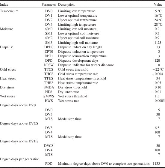
Values for parameter settings for the CLIMEX® model for projecting the distribution and density of S. mosellana populations in Europe and North America are listed in Table 1.
Values for parameter settings for the CLIMEX® model for projecting distribution and relative abundance of Sitodiplosis mosellana in Europe and North America.

Temperature: Weekly maximum and minimum temperature data were used to calculate development rates. Development rates were based on four parameters: DV0, DV1, DV2, and DV3. DV0 represents the lower temperature threshold, DV1 and DV2 describe lower and upper optimal temperatures, respectively, and DV3 defines the limiting high temperature threshold. Larval activity, indicating the termination of diapause, began in early May in Melfort, Saskatchewan (Doane and Olfert Reference Doane and Olfert2008). Larval diapause is terminated when spring temperatures exceed 3 °C and larvae become active at 6 °C. Based on geographic distribution, the lower temperature threshold for development was set to a value of 5 °C as reported by Elliott et al. (Reference Elliott, Mann and Olfert2009), who showed that it provided a more accurate estimate of adult emergence than base temperatures above 0 °C, 3–6 °C, 6 °C, and 9 °C. In Saskatchewan, adult flight occurs in late June or early July and mature larvae drop from wheat heads in early August. Developmental parameters were set at DV1=16 °C and DV2=24 °C to represent mid-summer adult and larval activity (Doane and Olfert Reference Doane and Olfert2008; Elliott et al. Reference Elliott, Mann and Olfert2009). Values for DV1, and DV2 were similar to those that were reported for swede midge, Contarinia nasturtii (Keiffer) (Olfert et al. Reference Olfert, Hallett, Weiss, Soroka and Goodfellow2006). The model used a value of 1135 degree-days for completion of one generation (Elliott et al. Reference Elliott, Mann and Olfert2009).
Moisture: The soil moisture index reflects the assumption that soil moisture is a significant factor that affects microclimatic conditions within the soil and plant canopy (Sutherst et al. Reference Sutherst, Maywald and Kriticos2007). Soil moisture parameters were inferred from reports of S. mosellana distribution in North America (Global Biodiversity Information Facility 2014). The level of S. mosellana infestation is related to total precipitation, with higher levels of infestations occurring during wetter growing seasons (Elliott et al. Reference Elliott, Mann and Olfert2009). Suitably moist soil conditions result in movement of larvae to the soil surface to pupate. Soil moisture was reported to be the main factor that determined diapause termination and pupation (Hinks and Doane Reference Hinks and Doane1988; Elliott et al. Reference Elliott, Mann and Olfert2009). When accumulated precipitation exceeds 20 mm in May, larvae terminate diapause, leave their cocoons and spend several days on the soil surface before pupating (Elliott et al. Reference Elliott, Mann and Olfert2009). Inadequate soil moisture can result in erratic emergence or extended diapause. Dry conditions during May or early June result in most larvae remaining dormant until the following year (Doane and Olfert Reference Doane and Olfert2008). Sites that received >145 mm of rain in May and June resulted in delayed emergence of adults (Elliott et al. Reference Elliott, Mann and Olfert2009).
Larval development of C. nasturtii is similar to that of S. mosellana, in that they enter a dormant state as a result of dry soil conditions. Dormancy was terminated in response to wetter soil conditions (Readshaw Reference Readshaw1966). Swede midge model parameters were used for initial moisture parameterisation (Olfert et al. Reference Olfert, Hallett, Weiss, Soroka and Goodfellow2006). Basedow and Schȕtte (Reference Basedow and Schȕtte1982) found that most S. mosellana larvae go into an extended diapause for another year when the soil moisture is <12%. In contrast, most larvae develop when the soil moisture reaches 17.5%. The limiting low threshold, SM0 was set at 0.2 and the lower optimal soil moisture, SM1, was set to 0.3. These values were required to accommodate S. mosellana distributions in southern Saskatchewan, Canada, and North Dakota and Montana, United States of America. Values for SM2 and SM3 were set to 0.9 and 1.25, respectively, in order to extend distribution to Québec, New Brunswick, and Nova Scotia, Canada (Borkent Reference Borkent1989).
Diapause: With adequate moisture, larval post-diapause development depends on temperature. Four parameters are used to define diapause: diapause induction day length (DPD0), diapause induction temperature (DPT0), diapause termination temperature (DPT1), and diapause development days (DPD). DPT0 was set to 3 °C in order to induce S. mosellana activity in the fall. Similarly, the diapause induction day length, DPD0, was set to 13 hours, representing day lengths that occur in early September in northern latitudes. These values produced results that indicated, for locations in northeastern Saskatchewan, larval activity would cease in mid to late September. This agreed with observations reported by Doane and Olfert (Reference Doane and Olfert2008) that larval cocoons were present in mid to late September. In the laboratory, S. mosellana larvae required 100 or more days to complete diapause with the highest emergence occurring after 120–160 days of exposure to cool temperatures (Wise and Lamb Reference Wise and Lamb2004). Our model used a value of 120 days in order to limit distributions between 42°N and 62°N (Affolter Reference Affolter1990). Using a DPT1 value of 3 °C agreed with reported observations for Saskatchewan (Doane and Olfert Reference Doane and Olfert2008). The DPT1 value of 3 °C resulted in expected distributions in Europe (Affolter Reference Affolter1990).
Stress indices: Abiotic stress indices reflect limitations associated with unfavourable conditions that occur outside of the growing season; stress indices accumulate outside the limits that permit population growth. In the case of S. mosellana, stress indices affect overwintering populations that are in the soil in the larval cocoon stage. Cold stress limits the northern range of S. mosellana distribution. The cold stress index is defined by two parameters: temperature threshold (TTCS) and rate of cold stress accumulation (THCS). Values of TTCS=−22 °C and THCS=−0.004 provided the best result for North America. Heat stress, wet stress, and dry indices had minimal impact on S. mosellana distribution or abundance. The dry stress threshold was set to 0.10 with an aggressive slope to indicate that stress would accumulate rapidly in extremely dry conditions. The wet stress threshold was set to 1.5 with a relatively flat slope to indicate that wet stress accumulation would be minimal.
Model validation
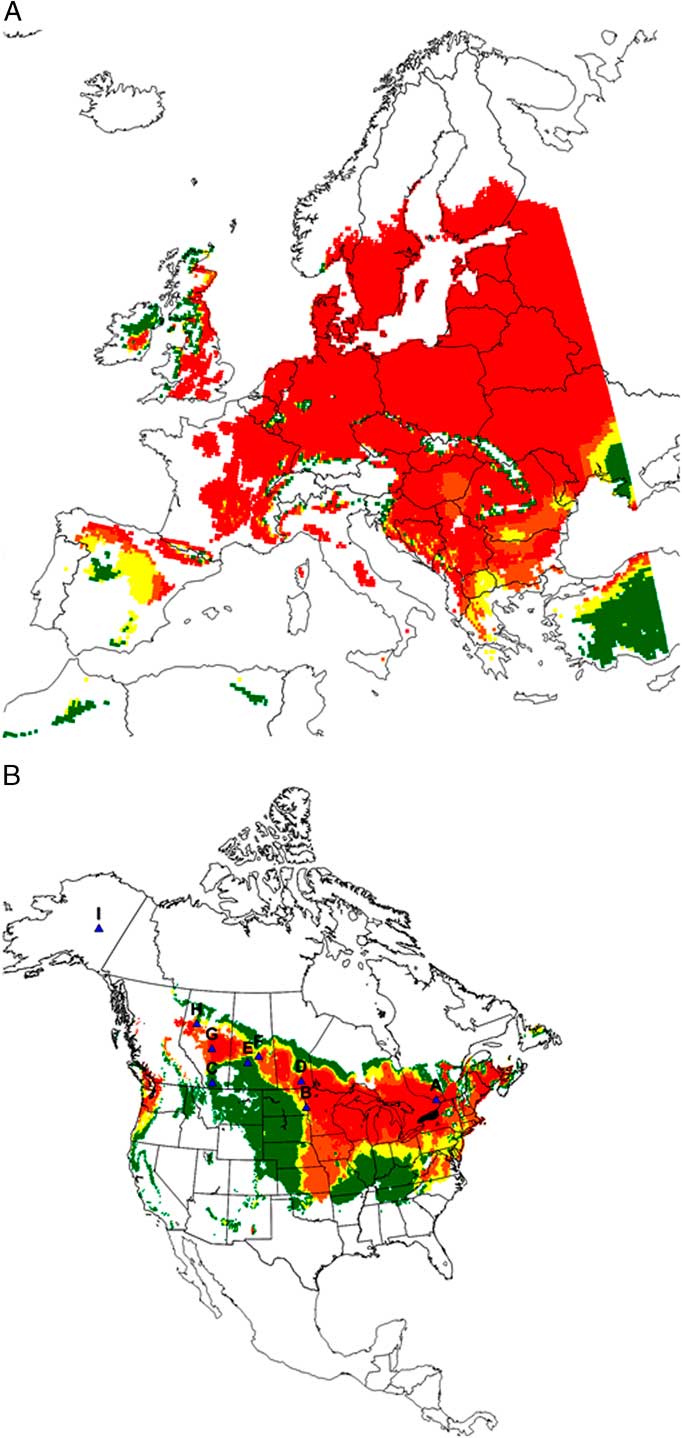
Distribution: Predicted distribution of S. mosellana (Fig. 1A) agreed with reported distributions for Europe, Asia and, North Africa (Wallengren Reference Wallengren1937; Speyer Reference Speyer1957; Braslavska Reference Braslavska1976; Skuhravy and Skuhrava Reference Skuhravy and Skuhrava.1978; Daamen Reference Daamen1981; Kurppa Reference Kurppa1989; Affolter Reference Affolter1990; Gao Reference Gao1995 as cited by Oakley et al. Reference Oakley, Cumbleton, Corbett, Saunders, Green and Young1998; European and Mediterranean Plant Protection Organization Global Database 2014; Fauna Europaea Web Service 2014). The distribution of S. mosellana overlaps wheat crop production areas in Northern Hemisphere as far north as wheat is grown; between 42°N and 62°N latitude. Internationally, S. mosellana has been reported from Algeria, Austria, Belgium, Bulgaria, China, Czech Republic, Denmark, Finland, France, Germany, Hungary, Ireland, Israel, Italy, Japan, Luxembourg, Montenegro, the Netherlands, Norway, Poland, Romania, Russia, Serbia, Slovakia, Sweden, Switzerland, Ukraine, and United Kingdom (European and Mediterranean Plant Protection Organization Global Database 2014; Fauna Europaea Web Service 2014). Though predicted to occur in Portugal (very limited distribution) and Spain, S. mosellana has not been reported from these countries.
Potential distribution and relative abundance of Sitodiplosis mosellana in Europe (A) and North America (B). Six regions were represented in North America: A – Ottawa, Ontario; B – Fargo, North Dakota; C – Lethbridge, Alberta; D – Winnipeg, Manitoba; E – Saskatoon, Saskatchewan; F – Melfort, Saskatchewan; G – Edmonton, Alberta; H – Peace River, Alberta; I – Fairbanks, Alaska. Ecoclimatic index values were presented in five categories: white=unfavourable (0–5); dark green=marginal (5–15); yellow=suitable (15–20); orange=favourable (20–25) and red=very favourable (>25).
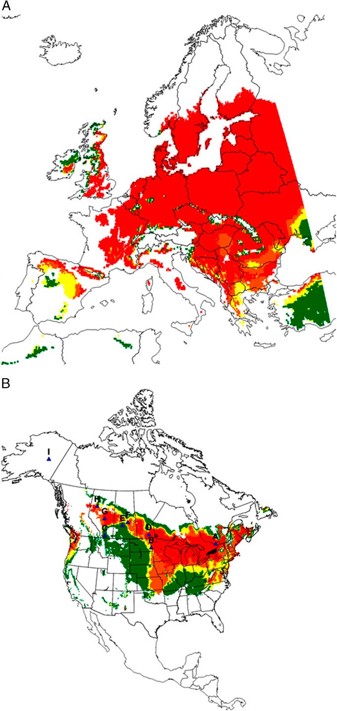
North American model output (Fig. 1B) agreed with reported distributions. Sitodiplosis mosellana most notably occurs across the northern Great Plains, including the Canadian prairies (Olfert et al. Reference Olfert, Elliott and Hartley2009). Canadian infestations were first reported from Québec in 1828 (Felt Reference Felt1921) and British Columbia in 1904 (Reeher Reference Reeher1945). Populations of S. mosellana have also been reported from numerous locations in Canada, including Alberta, Manitoba, New Brunswick, Nova Scotia, Ontario, and Saskatchewan (Olfert et al. Reference Olfert, Elliott and Hartley2009), and was recently reported from the Peace River region of Alberta (Western Committee on Crop Pests 2011). This species has also been reported from a number of states south of Canada including California, Idaho, Indiana, Michigan, Minnesota, Missouri, Montana, New York, North Dakota, Ohio, Oregon, and Washington (European and Mediterranean Plant Protection Organization Global Database 2014). The model predicted that S. mosellana could occur in a number of states in which the species has not yet been recorded, including Arkansas, Arizona, Connecticut, Iowa, Kansas, Maine, Massachusetts, New Hampshire, New Jersey, New Mexico, Pennsylvania, Utah, Vermont, Virginia, West Virginia, Wisconsin, and Wyoming. The lack of agreement between reported and modelled distribution does not necessarily indicate that the model is inaccurate. Lack of records for states that the model predicted as climatically suitable may be explained by lack of introduction of the species, environmental or demographic stochasticity, poorly suited hosts or lack of appropriate search effort (Kriticos et al. Reference Kriticos, Morin, Leriche, Anderson and Caley2013).
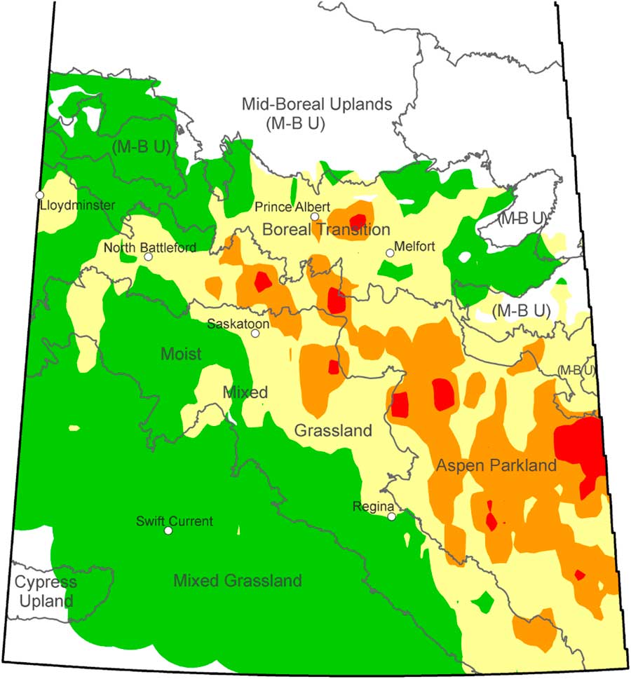
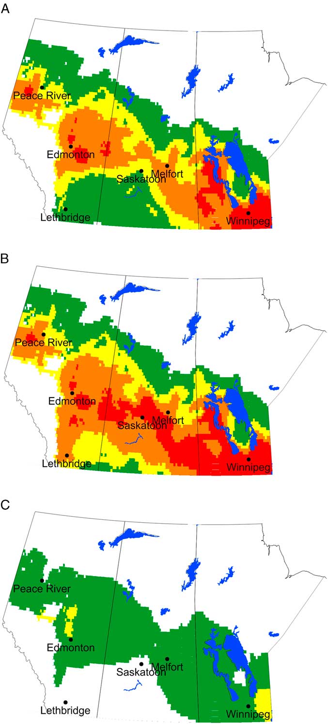
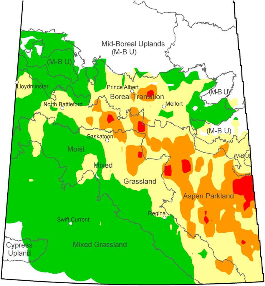
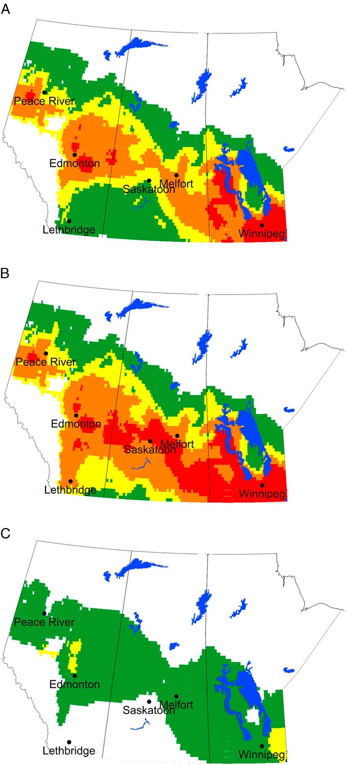
The model predicted that S. mosellana would occur throughout the wheat-growing region of Manitoba and was in agreement with survey results that were conducted in Manitoba between 1993 and 1997 (Lamb et al. Reference Lamb, Wise, Olfert, Gavloski and Barker1999). Modelled distribution also compared well with long term surveys of S. mosellana populations conducted in Saskatchewan (Olfert et al. Reference Olfert, Elliott and Hartley2009). They presented a series of annual maps (1991–2000) that demonstrated that midge populations were greatest across eastern and northern regions of the province over the 10-year period. A composite map for Saskatchewan (1991–2012) was developed to represent average larval cocoon density (Fig. 2). The economic threshold is ~1200 cocoons/m2 (Saskatchewan Ministry of Agriculture 2014). Results indicated that the risk of S. mosellana infestations is greater in eastern and northern regions, particularly the aspen parkland ecoregion, than west central and southern areas of the province. Predicted distribution and relative abundance was very similar to observed data (Fig. 2, Fig. 3A) and permitted a direct comparison between infestation thresholds and EI values. Comparison of Figs. 1B, 3A with Fig. 2 indicated that areas with EI values of 15 or greater are at risk from damage associated with S. mosellana (1200 cocoons/m2). Comparing temperature and rainfall climate data (1 May to 31 August) indicated that current distribution of S. mosellana occurs where climatic conditions are relatively moist and cool. The comparison of S. mosellana density (1991–2012) and climate data suggested that their densities were greatest in areas with total rain of 213–262 mm (specifically 243–262 mm) of rain with a growing season temperature of 14.0–15.2 °C. Precipitation scenarios were run to determine model sensitivity to precipitation. As expected, the predicted distribution and relative abundance of S. mosellana increased with wetter than normal conditions (20% above normal) and values decreased with dryer than normal conditions (20% less than normal) (Figs. 3B, 3C).
Average abundance (per m2) of Sitodiplosis mosellana larval cocoons in Saskatchewan during 1991–2012. Larval cocoons (per m2) are represented as: green=0–600; yellow=600–1200; orange=1200–1800; red⩾1800 larval cocoons/m2.
Predicted ecoclimatic index (EI) values for Sitodiplosis mosellana in western Canada for current climate (A), precipitation levels that are 20% greater than current climate (B) and precipitation levels that are 20% less than current climate (C). Ecoclimatic index values were presented in five categories: white=unfavourable (0–5); dark green=marginal (5–15); yellow=suitable (15–20); orange=favourable (20–25) and red=very favourable (>25).
Development and seasonal phenology: Model phenology was compared with field observations to confirm initiation of activity in spring and termination of activity in the fall. In northeastern Saskatchewan, larvae became active in early May and enter diapause in late September (Doane and Olfert Reference Doane and Olfert2008). Model runs for Melfort, Saskatchewan (52.9°N, 104.7°W), predicted that larvae would become active in mid-May and become inactive by late September. There was an accumulation of 1350 degree-days, exceeding the minimum requirement of 1135. The threshold and degree-day values allowed suitable EI values for northeastern Saskatchewan and Peace River, Alberta.
The model accurately predicted early spring activity in Europe. At Lund, Sweden (55.7°N, 13.2°E), S. mosellana larvae were reported to be active in April (Wallengren Reference Wallengren1937). The model predicted that S. mosellana would become active in late April, after accumulating 1525 degree-days. Adults appeared in May or June in Slovakia and this result agrees with model output (Braslavska Reference Braslavska1976). Based on comparisons between results reported for field studies and model output, results confirmed that the model is accurate in terms of threshold temperature (DV0=5), and degree-day value required to complete one generation (PDD=1135).
Stress indices: Comparable to reports by Wise and Lamb (Reference Wise and Lamb2004), model results suggested that S. mosellana mortality related to CS would be minimal across most of its current range. At Melfort, Saskatchewan, CS was predicted to accumulate for 20 days, with about 105 days with temperatures less than −10 °C, indicating <20% overwintering mortality. In a laboratory study, Wise and Lamb (Reference Wise and Lamb2004) reported that larval survival declined after 120 days at −10 °C.
Climate change: range and relative abundance of North American insects
Range shifts, contractions, expansions, and changes in relative abundance resulting from climate change, have been predicted for a number of North American insect species that are associated with agricultural ecosystems (Olfert and Weiss Reference Olfert and Weiss2006; Mika et al. Reference Mika, Weiss, Olfert, Hallett and Newman2008; Olfert et al. Reference Olfert, Weiss and Kriticos2011, Reference Olfert, Weiss, Turkington, Beckie and Kriticos2012). Species range shifts have been predicted to show range expansion in a north or northwestward direction and often associated with range contraction in the south. A study of three crop pests (weed, plant disease, and insect) in North America, Kochia scoparia (Linnaeus) Shrader (Amaranthaceae), Fusarium graminearium Schwabe (Nectriaceae), and Oulema melanopus (Linnaeus) (Coleoptera: Chrysomelidae) demonstrated range expansions to the north and contractions in the south, as a result of climate change (Olfert et al. Reference Olfert, Weiss, Turkington, Beckie and Kriticos2012). Projected range expansion was attributed to reduced cold stress and warmer temperatures resulting in sufficient heat to satisfy degree-day requirements while range contraction in the south was associated with heat and dry stress.
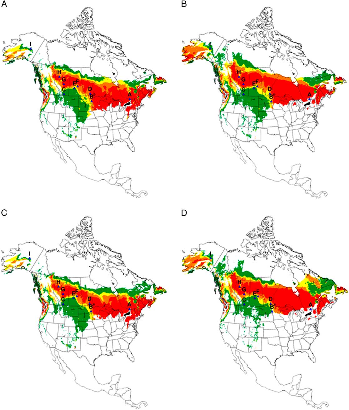
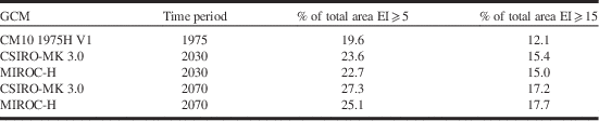
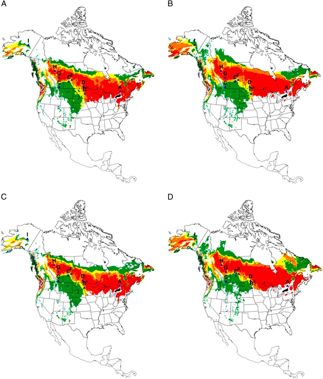
Results indicated that changes in EI values for S. mosellana were greatest between GCM time periods (current, 2030, and 2070) (Table 2). Values of EI>5 indicated regions where climatic conditions satisfied the ecological requirements of S. mosellana and would allow it to establish. Projections for 2030 and 2070 resulted in population range increasing from 19.6% of North America (current climate) to 23.6% (CSIRO-MK 3.0 2030) and 27.3% (CSIRO-MK 3.0 2070) (Table 2). Compared to EI>5, EI>15 provided a clearer estimate of potential distribution changes and response of relative abundance as a result of climate change. Based on comparison of Saskatchewan survey results (1991–2012) with model output for current climate, values of EI>15 were associated with regions where wheat crops were predicted to be at risk from S. mosellana damage (Figs. 2–3). Currently, this region (EI>15) extended across the northern United States of America, across the northern plains of Canada encompassing 12.1% of North America (Table 2, Fig. 1B). Projections for 2030 showed that regions with EI>15 will shift northward with large portions of the Canadian prairie, northern British Columbia, and isolated areas in Alaska having climates that would be conducive to S. mosellana outbreaks (Figs. 4A, 4C). By 2030, areas with EI>15 were predicted to increase to 15.4% for the CSIRO-MK 3.0 2030 GCM (Table 2). Species response to climate change may be reflected by changes in EI, changes in distribution or a combination of both. Compared to 2030, projections for 2070 resulted in moderate changes in EI and more significant changes in distribution with range expansion in areas north of 60°N and contraction in the southern limits of range for current climate (Figs. 4B, 4D). Predictions for 2070 suggested that 17.7% (MIROC-H 2070) of North America would have EI>15 (Table 2).
Potential distribution and relative abundance of Sitodiplosis mosellana in North America based on CSIRO-MK 3.0 general circulation model projections for 2030 (A) and 2070 (B) and MIROC-H general circulation model projections for 2030 (C) and 2070 (D). Nine regions were represented in North America: A – Ottawa, Ontario; B – Fargo, North Dakota; C – Lethbridge, Alberta; D – Winnipeg, Manitoba; E – Saskatoon, Saskatchewan; F – Melfort, Saskatchewan; G – Edmonton, Alberta; H – Peace River, Alberta; I – Fairbanks, Alaska. Ecoclimatic index values were presented in five categories: white=unfavourable (0–5); dark green=marginal (5–15); yellow=suitable (15–20); orange=favourable (20–25) and red=very favourable (>25).
Per cent of total geographic area where ecoclimatic index (EI) values for Sitodiplosis mosellana were EI⩾5 and EI⩾15 for current climate (CM10 1975H V1) and two general circulations models (CSIRO-MK3.0 and MIROC-H; 2030 and 2070).

Consideration must be given to the viability of agriculture, based on climate and soil constraints, in northern regions of North America. The potential for pest outbreaks could occur in south and central regions of Alaska where cereals are currently grown (Quarberg et al. Reference Quarberg, Jahns and Chumley2009). Interestingly, S. mosellana populations were recently reported as far north as Peace River, Alberta (56.2°N, 117.3°W) (Western Committee on Crop Pests 2011). Our model predicted that S. mosellana could expand its range even further to regions of northern North America where cereal crops are not currently grown (Canada Grain Commission 2012). However, in a study of arable soils in North America (55°N, 110°W) under a changing climate (+3.8 °C; +17% precipitation), Mills (Reference Mills1994) predicted that there would be an increase in available arable land (including cereal production) equal to the amount currently under cultivation within the prairie ecosystem. Similar to our study, sensitivity of land suitability was shown to be greatest in regions that are at the margins of cultivation (Ramankutty et al. Reference Ramankutty, Foley, Norman and McSweeney2002). They showed that high sensitivity to temperature occurred in southern regions of Canada, as well as northwestern and north central United States of America; precipitation was greatest in the Great Plains regions of the United States of America. Based on estimates for the years 2070–2099, they stated that there would be an increase of 16% of suitable cropland, specifically an increase of 1.5 million km2 in Canada. Our model predicted a 17.7% (MIROC-H 2070) increase in area for EI>15.
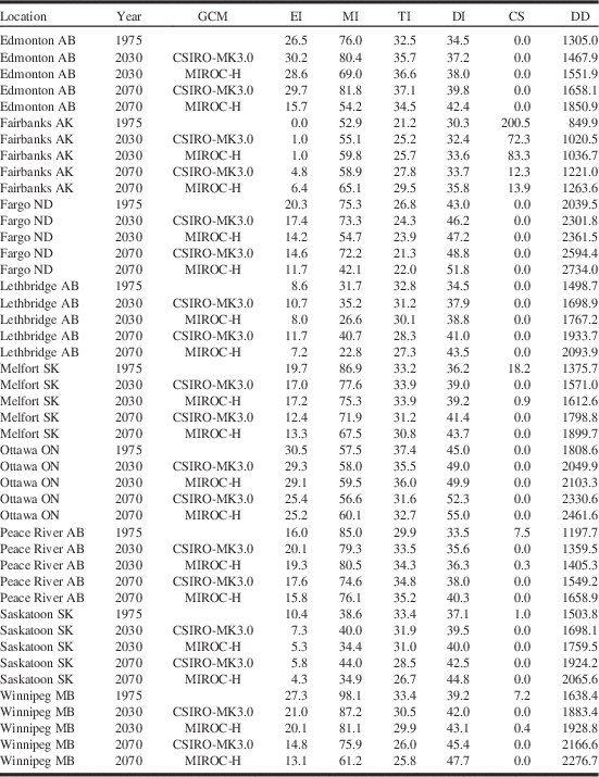
Differences between the two GCMs (MIROC-H and CSIRO-MK 3.0) were specific to particular regions in North America (Table 2) suggesting model sensitivity to GCM selection used for model input. Regional differences, related to GCMs, were previously reported for M. sanguinipes response to climate change (Olfert et al. Reference Olfert, Weiss and Kriticos2011). Mika et al. (Reference Mika, Weiss, Olfert, Hallett and Newman2008) reported that predictions of C. nasturtii response to variable climate was strongly dependent on the choice of GCM and suggested that multiple GCMs be used when studying species response to climate change. Based on projections for 2070, EI values at Edmonton and Lethbridge, Alberta, were markedly different between the two GCMs with MIROC-H (2070) predicting lower EI values. CSIRO-MK 3.0 predicted EI=29.7 for Edmonton, compared to EI=15.7 by MIROC-H (Table 3). For both locations, MI values were lower for MIROC-H. This reinforced the inference that the model is very sensitive to moisture.
Comparison of ecoclimatic index (EI), temperature index (TI), moisture index (MI), diapause index (DI), and cold stress (CS) for Sitodiplosis mosellana at nine locations in North America for current climate (CM10 1975H V1) and climate change scenarios (GCM) CSIRO-MK3.0 and MIROC-H; 2030 and 2070.

Note: AB, Alberta; AK, Alaska; MB, Manitoba; ND, North Dakota; ON, Ontario; SK, Saskatchewan.
Species vulnerability to temperature and precipitation is greater near the outer limits of their geographic range than at the core of their range. The core area is a region with high EI and minimal stress (Sutherst et al. Reference Sutherst, Maywald and Kriticos2007). In a comparison between current and future climates, M. sanguinipes populations near the core area were shown to have higher and less variable EI values than for populations near the outer limits of their geographic range (Olfert et al. Reference Olfert, Weiss and Kriticos2011). Results, based on CSIRO-MK 3.0 and MIROC-H, indicated that locations near the core, for example Melfort, Saskatchewan, exhibited minimal change in EI between current and future climates. Locations near the outer limits of the current modeled distribution were more sensitive to changes in future climates than locations near the central core (Table 3).
Sitodiplosis mosellana has not yet been reported from the Fairbanks region of Alaska (64.8°N, 147.7°W); although growing season temperatures (TI) and moisture (MI) levels are currently comparable to Edmonton, Alberta. The model predicted that degree-day requirements were insufficient (current climate and 2030) or marginal (2070) and that cold stress-related (CS) mortality did not permit the species to successfully overwinter in central Alaska (Table 3). Projections for 2070 indicated that TI and MI values would increase marginally; increased EI values were associated with decreased CS values and degree-day accumulations that exceeded the threshold (PDD=1135). Model projections for 2070 suggested cold stress values would decrease to CS=0 (CSIRO-MK 3.0), which is less than CS=18.2 for current climate at Melfort, Saskatchewan. Both GCMs predicted that EI values south and west of Fairbanks, Alaska will be categorised as “Favourable” (EI=20–25) or “Very Favourable” (EI>25) by 2070 (Figs. 4B, 4D). The values presented in Table 3 appear to underestimate EI values. Figures 4B, 4D indicate that EI values are greater than this. The reason for the difference is that it is an artifact of the averaging (over ±1 degree latitude and longitude) around Fairbanks, Alaska.
In contrast to northern expansions, the model indicated that EI values will decrease along the southern limits of the species current range. For example, at Fargo, North Dakota, EI=20.3 for current climate, suggesting potential for crop loss from S. mosellana. By 2070, warmer temperatures, affecting diapause induction/termination and lower MI, resulted in a decrease to EI=11.7 (MIROC-H). Similar trends were predicted to occur for Saskatoon, Saskatchewan. Range contractions across the southern distribution limits were greatest for the 2070 time period. The southern limit for current climate was approximately 35°N latitude. Projections for 2030 indicated a northward shift to 37°N for both GCMs. Projections for 2070 predicted that the southern limits would recede to 38°N and 40.5°N for CSIRO-MK 3.0 and MIROC-H, respectively.
Natural enemies of Sitodiplosis mosellana
In summary, the study found that the range and abundance of S. mosellana, and associated crop risk, was predicted to expand in a northerly direction and diminish across the present southern limits under a changing climate. In addition to the abiotic factors (climate variables), there may also be biotic factors that influence the relative distribution and abundance of S. mosellana populations in the future, such as biological control agents. The parasitoid, Macroglenes penetrans (Kirby) (Hymenoptera: Pteromalidae), currently plays a significant role in reducing S. mosellana infestations on the northern Great Plains. In Saskatchewan, >95% of wheat fields infested with S. mosellana had some level of parasitism, averaging 20–45% across the province annually (Olfert et al. Reference Olfert, Elliott and Hartley2009). In 1993 and 1994, a second biological control agent, Platygaster tuberosula Kieffer (Hymenoptera: Platygastridae) was introduced to further enhance biological control of S. mosellana in Saskatchewan (Doane et al. Reference Doane, Mukerji and Olfert2000; Olfert et al. Reference Olfert, Elliott and Hartley2009).
Though our model predicted that the distribution and relative abundance of S. mosellana would change in many regions of North America, model output based on EI values, indicated that S. mosellana densities in Manitoba, Saskatchewan, and Alberta would continue to have similar ranges and densities in 2030 and 2070. This suggests that M. penetrans and P. tuberosula should continue to serve as biological control agents for S. mosellana. Relative to pest insect species, few bioclimatic models have been developed for biological control agents. Bioclimatic models, integrated with the S. mosellana model, should be developed in order to gain a better understanding of the impact of climate change on these two parasitoid species.
Acknowledgements
The authors would like to acknowledge the collaborators and funding agencies of the Prairie Pest Monitoring Network and Saskatchewan Crop Insurance for seasons of S. mosellana population monitoring. Thanks to D. Giffen for preparation of the maps.