


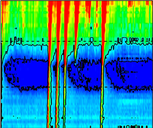

1. Introduction
Laminar-turbulent transition has a critical effect on the aerothermodynamics of hypersonic flight and as such is the subject of extensive research, both experimental and computational. Classic test cases include the flat plate (e.g. Franko & Lele Reference Franko and Lele2013; Chuvakhov, Fedorov & Obraz Reference Chuvakhov, Fedorov and Obraz2018) and the sharp cone (e.g. with half-angles of 5 $^\circ$–7
 $^\circ$ in Sivasubramanian & Fasel Reference Sivasubramanian and Fasel2015; Hader & Fasel Reference Hader and Fasel2019). The Hypersonic International Flight Research Experimentation (HIFiRE)-5b has documented transition on a sharp-nose vehicle (Kimmel et al. Reference Kimmel, Adamczak, Hartley, Alesi, Frost, Pietsch, Shannon and Silvester2018) from heat flux measurements, including turbulent overshoots and defining a connection between transition length and turbulent spot generation rates (Juliano, Jewell & Kimmel Reference Juliano, Jewell and Kimmel2021). Other geometries, including concave surfaces and swept leading edges, are broadly relevant to hypersonic vehicle design (e.g. the Skylon concept spaceplane, ESA 2011) and are as well notably being considered under the Boundary Layer Transition (BOLT) flight experiment (Wheaton et al. Reference Wheaton, Berridge, Wolf, Araya, Stevens, Mcgrath, Kemp and Adamczak2021). The mechanisms of transition in blunt bodies, such as blunt cones or re-entry capsules, present a number of distinct characteristics that render them difficult to predict (Leidy et al. Reference Leidy, Reshotko, Siddiqui and Bowersox2017; Paredes, Choudhari & Li Reference Paredes, Choudhari and Li2020a). Regions involving flow separation are commonplace, but the physics of separated transitional boundary layers remains less well understood. The objective of this work is to establish a two-dimensional (axisymmetric) laminar separation, over a blunt body of revolution at Mach 9, which is then perturbed by incoming turbulent spots.
Transition to turbulence can occur through different mechanisms, ranging from modal growth of relatively weak boundary layer instabilities – such as Görtler vortices, cross-flow instabilities, first and second Mack modes (Mack Reference Mack1984) – to strong disturbances that bypass the more moderate processes and abruptly trip the flow to a turbulent state (Reshotko Reference Reshotko2001). Short roughness elements can introduce transient perturbations that are nonlinear in nature and that may grow to prompt transition (Tumin Reference Tumin2007), while taller ‘effective’ elements force transition at a finite distance close downstream within their wake, in which case absolute instability is likely to dominate (Wheaton et al. Reference Wheaton, Bartkowicz, Subbareddy, Schneider and Candler2011). Theoretical models of transient growth for roughness-induced transition generally rely on analysis of optimal perturbations, associated with the streamwise vortices in the element's wake, aided by empirical correlations (Tumin Reference Tumin2008). Further efforts to model the receptivity of the boundary layer, in terms of kinetic fluctuations in the associated stress tensors and heat fluxes, have gone to characterise the generated small-scale flow perturbations and their amplification via nonlinear effects towards transition (Fedorov & Tumin Reference Fedorov and Tumin2017). Detailed insight on the various transition pathways of high-speed flows may be found in the reviews by Schneider (Reference Schneider2008) and Fedorov (Reference Fedorov2011), and more recently by Lee & Jiang (Reference Lee and Jiang2019).
The present investigation falls within an intermediary stage in which laminar disturbances with significant amplitude experience transient growth and bypass the earlier mentioned mechanisms to break down into patches, or spots, of turbulent flow. Turbulent spots are key elements in the classical transition process and were identified originally in incompressible flow studies by Emmons (Reference Emmons1951). They generally exhibit a characteristic arrowhead planform that is understood to be a result of a ‘cascading’ effect whereby upstream disturbances foster the development of new disturbances as the spot convects in the streamwise direction (Perry, Lim & Teh Reference Perry, Lim and Teh1981). Turbulent spot growth is thus inherently influenced by classical entrainment as well as by destabilisation of the surrounding laminar flow, with lateral spreading rates substantially greater than the wall-normal growth (Gad-El-Hak, Blackwelder & Riley Reference Gad-El-Hak, Blackwelder and Riley1981). Retardation of the near-wall flow induces a growing streamwise elongation of the spot, leading to coalescence with neighbouring spots and the eventual formation of fully turbulent flow (Narasimha Reference Narasimha1985).
As depicted in figure 1, the internal organisation of well-developed spots exhibits a front overhang region, followed by a turbulent core with lateral wing tips and a calmed wake at its rear. The overhang and wing tip organisation is driven by near-wall flow retardation, and the calmed region behind the arrowhead structure is more elongated near the centreline. Fischer (Reference Fischer1972) showed that the lateral growth rate of turbulent jets/wedges decreased with increasing supersonic Mach number, and such low spreading rates have been observed consistently for turbulent spots in hypersonic experiments, including Mee (Reference Mee2002), Casper, Beresh & Schneider (Reference Casper, Beresh and Schneider2014) and Jewell, Leyva & Shepherd (Reference Jewell, Leyva and Shepherd2017) as well as those preceding the present investigation (Fiala et al. Reference Fiala, Hillier, Mallinson and Wijensinghe2006; Fiala, Hillier & Estruch-Samper Reference Fiala, Hillier and Estruch-Samper2014). Direct numerical simulations (DNS) by Krishnan & Sandham (Reference Krishnan and Sandham2006, Reference Krishnan and Sandham2007) and Redford, Sandham & Roberts (Reference Redford, Sandham and Roberts2012) have shed light on the mechanisms for formation of new disturbances and on the spot substructures. Krishnan & Sandham (Reference Krishnan and Sandham2007) also used computational fluid dynamics (CFD) to study the effect of turbulent spots on a shock-wave-induced separation and found that the associated adverse pressure gradient has a generally destabilising influence on the spot, in agreement with earlier observations from incompressible flows (Seifert & Wygnansky Reference Seifert and Wygnansky1995). This was corroborated in the hypersonic tests by Butler & Laurence (Reference Butler and Laurence2020) on a 5 $^\circ$ half-angle cone, where it was observed that corner flow separation over a 15
 $^\circ$ half-angle flare promoted rapid breakdown of instability waves upon reattachment, while expansion regions had a stabilising effect on the disturbances.
Schematic of turbulent spot substructures based on the conceptual model by Perry et al. (Reference Perry, Lim and Teh1981). Spot with origin at the inception location  $x_o$.

DNS has proven a particularly useful tool to provide insights of hypersonic transition where ground testing may be challenged to obtain non-intrusive information at high spatial resolution. In Franko & Lele (Reference Franko and Lele2013), the development of streamwise streaks and their breakdown to fully turbulent flow was investigated for a Mach 6 flat plate boundary layer, noting a heat transfer overshoot similar to the tendencies observed in past experiments; and likewise Sivasubramanian & Fasel (Reference Sivasubramanian and Fasel2015) established that the fundamental breakdown to turbulence is a viable mechanism in sharp cone configurations at the same Mach number. Novikov, Egorov & Fedorov (Reference Novikov, Egorov and Fedorov2016) conducted DNS of three-dimensional (3-D) wave packets over a Mach 5.4 compression corner, and found that nonlinear effects could destabilise the wave packet in the separation region and lead to its breakdown downstream of reattachment, prompting the formation of a young turbulent spot in the reattached flow region when sufficiently strong forcing was applied; the authors concluded that the wave packet contents and its downstream evolution depend strongly on how and where the initial disturbance is excited. Along these lines, Chuvakhov et al. (Reference Chuvakhov, Fedorov and Obraz2018) assessed the suitability of different unsteady boundary conditions for DNS modelling of the nonlinear breakdown of unstable wave packets into turbulent spots over a Mach 6 flat plate boundary layer. And Hader & Fasel (Reference Hader and Fasel2019) further resolved the formation of streamwise high skin-friction and heat-transfer streaks over a flared cone at the same Mach number, arguing that the fundamental breakdown to turbulence is likely to be a dominant path to transition under low-noise (‘quiet’) conditions.
Recent ground test studies have, on the other hand, looked into the fluid–structure interaction associated with the passage of turbulent spots. In the experiments by Casper et al. (Reference Casper, Beresh, Henfling, Spillers, Hunter and Spitzer2018) on a 7 $^\circ$ half-angle cone at Mach 5–8, the surface response to the passage of spark-generated spots was characterised by accelerometers on the backside of a panel. Under ‘quiet’ Mach 6 conditions, the flow remained laminar and spots excited a directionally-dependent panel response, but this was masked by acoustic perturbations in other higher-noise facilities, where a clear structural response was seen only for spot passage rates near the natural frequency of the panel. Subsequent studies on a slender cone found good agreement between numerical estimates of the cone structural response and experimental damping times and acceleration amplitudes (Robbins, Casper & Mesh Reference Robbins, Casper and Mesh2019), again concluding that higher rates of spot generation lead to enhanced response near the structure's natural modes. Similar observations were noted by Whalen et al. (Reference Whalen, Schoneich, Laurence, Sullivan, Bodony, Freydin, Dowell and Buck2020) in their experimental tests on a flexible panel exposed to a Mach 6 ramp-induced shock-wave/boundary-layer interaction.
Within the context of transition in hypersonic blunt bodies, significant progress in the understanding of discrete roughness effects and relevant correlations was made during the Shuttle programme (Berry & Horvath Reference Berry and Horvath2008; Horvath et al. Reference Horvath, Zalameda, Wood, Berry, Schwartz, Dantowitz, Spisz and Taylor2012). More recently, Leidy et al. (Reference Leidy, Reshotko, Siddiqui and Bowersox2017) considered the transition over a blunt body modelled after the Orion capsule at re-entry conditions and related the local flow properties and roughness heights to established transient growth scalings; while Radespiel et al. (Reference Radespiel, Ali, Munoz, Bowersox, Leidy, Tanno, Kirk and Reshotko2018) assessed the effects of roughness over spherical Apollo-type capsule models for a range of experimental studies at different hypersonic facilities, finding good evaluation against transient growth theory and numerical simulation data. DNS of transition over similar re-entry capsules has provided insights into the generation of stationary roughness-induced disturbances and the evolution of unsteady perturbations (Hein et al. Reference Hein, Theiss, DI Giovanni, Stemmer, Schilden, Schroder, Paredes, Choudhari, LI and Reshotko2019). Yet, as noted by Paredes et al. (Reference Paredes, Choudhari and Li2020a), the planar Mack-mode instabilities that more commonly dominate transition in sharp cone geometries can suffer a reduction in modal growth in blunt configurations, yielding a more complex environment where both planar and oblique convecting disturbances may experience substantial amplification. The presence of separation regions as in the present case inevitably adds to the complexity of the problem.
2. Computational and experimental details
2.1. Computational method
The geometric details of the test model are provided in figure 2. Everywhere the attached (pre-separation) boundary layer is less than 2 mm thick, making experimental profile or thickness measurements non-viable. Similarly, there were no means available to measure separation and reattachment positions accurately. These are all critical defining elements for separated flow studies, however, so that laminar CFD has been employed to provide support to the experimental work. It also provided a central role in the initial model design decisions.
Test geometry. Body of revolution with spherically blunted nose, radius  $R_{N} = 25$ mm, blended by an arc, radius
 $R_{B} = 273$ mm, to a cylindrical section of diameter
 $D = 75$ mm. The blending-arc/cylinder junction (
 $x_{j}$) is at 103 mm. Design iteration selected an
 $8^\circ$ angle flare (
 ${\alpha }_{f}$) with cylinder–flare junction (
 $x_{f}$) at 212 mm. The axial separation and reattachment positions,
 $x_{S}$ and
 $x_{R}$, are estimated as 200.5 mm and 223.5 mm, respectively. The roughness element location (
 $x_{k}$) is 38 mm. Long-dashed lines show an idealisation for the trajectory of spot formation, with an effective origin close to
 $x_{j}$.

A second-order (space and time) finite-volume code was used, assuming axial symmetry, with a mesh of quadrilateral cells in the ( $x,r$)-plane. A generalised Riemann problem (Ben-Artzi & Falcovitz Reference Ben-Artzi and Falcovitz1984; Hillier Reference Hillier2007) provided inviscid fluxes at cell interfaces with centred differencing used for the diffusive terms. It is time-marched to steady state from an impulsive start at free stream conditions. An adaptive mesh strategy was used to refine resolution in important areas. The finest mesh (A) used 1000 cells along the body surface from the stagnation point to a chord distance of 250 mm, with 140 cells covering the predicted 23 mm distance from separation (
 $x_{S}$ in figure 2) to reattachment (
 $x_{R}$). It also provided, over the full chord length, both 500 cells from the body surface to the bow shock wave and also a minimum of 110 cells from the body surface to the outer edge of the viscous layer. At the cylinder–flare junction position, virtually at mid separation length, converged results showed that there were 48 cells from the surface out to the maximum reverse flow position, a further 30 cells to reach the separation streamline, and a further 45 cells to reach the edge of the free shear layer. Clearly, confirmation of mesh convergence is important, and mesh B was generated by combining local clusters of four cells, from mesh A, into one cell, with mesh C resulting from a similar coarsening of mesh B. Heat transfer is a sensitive measure of mesh convergence, and the CFD results, in figure 3(b), show that predictions for meshes A and B are virtually indistinguishable; only downstream of reattachment (
 $x \approx 230$ mm) is a difference visible of approximately 1.5 %. Mesh C, the coarsest option, shows a visible, but still slight, difference. For pressure (figure 3a), the meshes A and B effectively overlay each other over the full chord range with practically no difference evident for mesh C. Thus mesh A is assumed to correspond very closely to the mesh-converged steady, laminar axisymmetric solution and provide the results presented.
Reference laminar data (no roughness element). (a,b) Flare case: axial distributions for mean surface pressure and heat transfer, experiment ( $\bigcirc$) and CFD (dashed-dot, dashed and solid lines for progressive mesh refinement from mesh C through mesh B to mesh A). Experimental surface pressure on the opposite side of the model to assess alignment (
 $\Delta$). No-flare case experiment (
 $\square$) and CFD with mesh A (long-dashed line). (c) Schlieren of separation zone. (d) Density contours from CFD.

2.2. Gun tunnel facility
The Imperial College gun tunnel uses Nitrogen test gas. Flow total pressure and temperature ( $P_{0,\infty }$,
 $T_{0,\infty }$) are monitored, and reproduced closely, from run to run, and are given in table 1. Flow characterisation is completed by Mach number definition, usually achieved through Pitot probe or static pressure probe measurements. Both can cause issues, and here the no-flare model was employed in a secondary role as a calibration probe. CFD (as described in § 2.1), using simulations at free stream Mach numbers,
 $M_{\infty }$, 8.9, 9.0 and 9.1, determined that a value of 9.025 gave the best fit to the measured no-flare surface pressure data. In such an approach it is essential that full Navier–Stokes simulations are employed since the boundary layer induced contribution to the pressure can be significant. This calibration ensured, of course, that surface pressures upstream of separation would match closely between CFD and experiment. This process used no further data measured on the model, be it surface heat transfer or data produced with the flare configuration. Detailed spatial calibration by Mallinson et al. (Reference Mallinson, Hillier, Jackson, Kirk, Soltani and Zanchetta2000) also showed a weak axial Mach number gradient that is barely significant for the present short chord model, causing only an approximate 4 % fall in static pressure along the model up to the end of the instrumented section at
 $x = 250$ mm. Total run duration is 25 ms, with an established flow window of approximately 6 ms. The Prandtl number
 $Pr$ is assumed constant at 0.72, and the viscosity is evaluated using Keyes (Reference Keyes1952). The full tunnel conditions used in data reduction and CFD are summarised in table 1.
Nominal flow conditions: free stream Mach number  $M_{\infty }$, axial Mach number gradient
 ${\rm d}M_{\infty }/{{\rm d}\kern0.7pt x}$, total free stream pressure
 $P_{0,\infty }$, total free stream temperature
 $T_{0,\infty }$, wall temperature
 $T_{w}$, and unit free stream Reynolds number
 $Re_{\infty }$.

2.3. Model and instrumentation
The basic no-flare model, that is, the blunt-nose-cylinder element of figure 2, already existed from earlier transition studies (Fiala et al. Reference Fiala, Hillier, Mallinson and Wijensinghe2006, Reference Fiala, Hillier and Estruch-Samper2014). The 25 mm nose radius  $R_{N}$ was chosen to be very large compared with the boundary layer thickness and almost completely avoids entropy layer ‘swallowing’ over the measurement length. The nose is blended to the cylindrical afterbody, diameter
 $D = 75$ mm, by a constant radius arc
 $R_{B}$ of 273 mm that maintains continuity of body slope at matching points
 $x=17.2$ mm and
 $x=103$ mm, and provides a monotonic fall of pressure from the nose stagnation point (
 $104 p_{\infty }$) to the test region over the cylinder body (
 $p \approx 1.6 p_{\infty }$), where
 $p_{\infty }$ is the free stream static pressure.
Table 2 lists reference properties at three salient  $x$ locations, for the no-flare case. These are:
 $x_{k}$ (38 mm), the final location selected for the use of the roughness element;
 $x_{j}$ (103 mm), the blending arc–cylinder junction; and
 $x_{f}$ (212 mm), the final selected position for the cylinder–flare junction. The table includes boundary layer thickness estimates extracted from the CFD. Since the flow is rotational between the boundary layer edge and the bow shock, edge conditions are taken at the predicted position of 99.5 % recovery of total enthalpy
 $h_0$ from the wall, that is,
 $(h_{0}-h_{w}) = 0.995(h_{0,\infty }-h_{w})$. Boundary layer thickness
 $\delta _x$, edge velocity
 $U_e$ and other edge properties are determined based on this definition.
Laminar CFD-evaluated reference properties for the no-flare model at roughness element location  $x_{k}$, nose–cylinder junction
 $x_{j}$, and cylinder–flare junction
 $x_{f}$. Properties include: edge Mach number
 $M_{e}$, unit Reynolds number with properties evaluated at boundary layer edge
 $Re_{e}$, edge to free stream velocity ratio
 $U_{e}/U_{\infty }$, edge to wall temperature ratio
 $T_{e}/T_{w}$, local boundary layer thickness
 $\delta _x$ (at given ‘
 $x$’ station), displacement and momentum thicknesses
 $\delta _{1,x}$ and
 $\delta _{2,x}$, laminar heat transfer
 $q_{L,x}$, and ratio of momentum thickness Reynolds number to edge Mach number
 ${ Re_{{\delta }_2}}/M_{e}$.

The cylinder–flare design addressed three constraints.
(1) Turbulent spots had to be well developed by the time they reached the measurement region and large enough to ensure satisfactory spatial resolution. As such, a minimum position for the cylinder–flare junction was enforced with
 $x_{f} \ge 200$ mm. By this stage, for the given roughness element conditions described in § 4.1, the spot width and length were expected to be respectively of orders 20–25 mm and 40–75 mm.
(2) The flare angle
${\alpha }_{f}$, and hence the separation scale, should be large enough for good resolution of the interaction. A minimum of 6$^\circ$ was enforced to ensure sufficient margin above the incipient separation angle.(3) The separation scale should be small enough to ensure full re-establishment, after spot-induced collapse, within the 6 ms tunnel test window.


Constraints (2) and (3) are in conflict, but (3) is the most critical, and a maximum establishment time of 2 ms was enforced. The design issues were addressed by a mix of schlieren visualisation of prototype models and time-accurate laminar CFD (§ 2.1) assuming an impulsive flow start. The final selection chose a ‘safe’ option of an 8 $^\circ$ flare located at
 $x_f = 212$ mm, giving a predicted separation length,
 $L_{S}$, of 23 mm. From the CFD the separation length establishes within 1
 $\%$ of its asymptotic value in 2 ms; experimentally, re-establishment was faster, probably because the simulation was axisymmetric while the actual process is three-dimensional.
Surface heat transfer measurements used platinum thin-film gauges on a Macor substrate as: (a) an axial array of up to 64 gauges pitched at 1 mm spacing and with sensor element size  $\Delta x = 0.1$ mm by
 $\Delta z = 2$ mm; and (b) an 18-gauge circumferential array spaced at 4 mm (6.1
 $^{\circ }$) in azimuth and with spatial resolution
 $\Delta z = 2.5$ mm. These sensors registered 90 % of a step change in surface heat transfer in 11
 $\mathrm {\mu }$s (Schultz & Jones Reference Schultz and Jones1973), and the measured surface temperature history was reduced digitally to heat transfer (Cook & Felderman Reference Cook and Felderman1966; Schultz & Jones Reference Schultz and Jones1973) with an estimated error of
 $\pm$10
 $\%$. Pressure measurements used Kulite XCS-062 miniature transducers located just below the surface, with a tapping diameter of 0.5 mm, as: (a) an axial array at a pitch of 2 mm; and (b) one axial array of sensors with a pitch of 4 mm, over the cylindrical section on the opposite side of the model, to aid alignment. The expected error in the pressure measurements is
 $\pm$3.5
 $\%$ with an estimated frequency response of 80 kHz for the tapping/dead-volume/transducer combination. Sensor outputs were amplified and low-pass filtered at 50 kHz before digitising through a 24-bit analogue-to-digital converter at a sample rate of 100 kHz.
3. Reference laminar separation
3.1. Model surface conditions and alignment with free stream
Considerable effort was made to ensure laminar conditions. The model was highly polished, its surface finish ensuring an average roughness <0.5  $\mathrm {\mu }$m, and the test section kept clean and free of contaminating particles between runs. Initially, it was found that turbulent spots could be triggered by disturbances produced by particles released at the initial rupture of the Melinex (polyester film) nozzle-throat diaphragms, so these were replaced by stainless steel diaphragms with a better rupture behaviour.
The model was aligned geometrically with the nozzle axis within  ${\pm }0.05^\circ$ in pitch and yaw and within 0.5 mm in translation. Figure 3(a) presents various data but the specific ones related to model alignment are the axial distribution of surface pressure from the main row of tappings (on the top of the model) together with the more restricted axial row at
 $180^\circ$ in azimuth (on the bottom). These cover both attached and separated flow segments. They show almost exact agreement between the two sets of tappings, and confirm excellent alignment of the model in pitch. It also supports the decision to use a body of revolution to produce the best possible two-dimensional (i.e. axisymmetric) flow. There were no tapping rows on each side of the model so aerodynamic alignment in yaw cannot be confirmed categorically although geometric alignment is as precise as in pitch.
3.2. Surface pressure and data normalisation
Axial distributions of average pressure and heat transfer are presented in figures 3(a,b) for tests on the blunt cylinder flare and the basic blunt cylinder body without the flare. From here on, they are referred to simply as the flare and no-flare cases. Because of the calibration process, experiment and CFD for pressure for the no-flare case (figure 3a) are essentially in precise agreement. For the flare case, the CFD predictions for pressure again agree closely with the measurements (figure 3a). It therefore seems most unlikely that the CFD-predicted positions for separation and reattachment should differ significantly from the actual experimental values. Therefore, in the absence of direct measurement of separation and reattachment positions and separation length ( $x_{S}, x_{R}, L_{S}$), all references to these refer to CFD-predicted values. These are given in table 3. It is difficult to place an accuracy estimate on this procedure. However, the small discrepancy between CFD and experiment places the initial measured separation pressure rise (
 $195 \le x\ ({\rm mm}) \le 205$) slightly upstream of the CFD prediction, while the measured reattachment rise is shifted (
 $215 \le x\ ({\rm mm}) \le 225$), by an even smaller amount, slightly downstream. This would amount potentially to an underestimate of experimental separation length by CFD of approximately 5 % or 1.2 mm.
Reference data for  ${\alpha }_{f}=8^\circ$ flare with cylinder–flare junction at
 $x_{f}= 212$ mm. The base laminar heat transfer and pressure
 $q_{L}$ and
 $p_{L}$ correspond to the undisturbed (attached) flow values taken from experiment at
 $x_{S}$ on the blunt cylinder without the flare. The remainder of values given are from CFD;
 $H_{S}$ is the normal distance from the cylinder–flare junction to the separation streamline, and
 $\delta _{1,L}$ is the displacement boundary layer thickness at
 $x_{S}$ (i.e.
 $x^{*}_{S} = 0$). Here,
 $x_{S}$ and
 $x_{R}$ are based on the zero skin-friction coefficient
 $C_f=0$ criterion.

In figure 3, and following, the axial distance ( $x$) is presented both in dimensioned form and also normalised by the CFD predicted separation/reattachment scales, so that
 $x^{*}_{S}$ values 0 and 1 correspond respectively to separation and reattachment. Similarly,
 $z^{*}_{S}$ and
 $y^{*}_{S}$ denote the transverse circumferential distance from the centreline, and the body normal distance, both normalised by
 $L_{S}$. Surface pressure (
 $p$) and heat transfer (
 $q$) are likewise presented in dimensioned form and also normalised by the reference values (
 $p_{L}$ and
 $q_{L}$), taken on the no-flare model but at the separation position identified for the flare case. These reference values are also listed in table 3. As a final observation on the pressure distribution, the lack of a clear plateau in the pressure distribution (between the separation and reattachment pressure rises) is characteristic of the separation length,
 $L_{S}$, being modest in scale compared to the boundary layer thickness,
 $L_{S}/{{\delta }_{0}} = 12.2$.
3.3. Surface heat transfer
Figure 3(b) shows a very close match between CFD and experiment for heat transfer for the no-flare case. For the flare case, however, CFD underpredicts heat transfer in three segments.
(1) There is a small (in amplitude and streamwise scale) effect centred at
$x^{*}_{S} \approx -0.4$, which is the position where the separation pressure rise begins (figure 3a).(2) In the separation zone, both CFD and experiment show a minimum at the same position (
$x^{*}_{S} \approx 0.35$), but CFD clearly underpredicts experiment.(3) Approaching reattachment, measured heat transfer rises well above CFD to reach a maximum at
$x^{*}_{S} \approx 1.5$, then falls rapidly with every likelihood of meeting the CFD distribution shortly beyond the end of the instrumented section.


Two critical assumptions in the CFD modelling are that the flow is both axisymmetric and laminar. Departure from axisymmetry due to incidence or yaw has been excluded previously. A 3-D effect (i.e. non-axisymmetry), which has appeared in separated flows over a broad range of Mach numbers, is streamwise cellular structures or Goertler-type vortices. Figure 4 presents a typical surface oil flow taken during a run. Clearly, there are issues with using oil flows in a short duration facility, and resolution was insufficient to produce features that could be identified as separation/reattachment, but it does indicate a series of streamwise structures with spanwise spacing about twice the pre-separation boundary layer thickness. Such structures have been identified in a range of separation studies, both laminar and turbulent, including the rearward-facing step (Roshko & Thomke Reference Roshko and Thomke1966), several studies in the present facility (Denman Reference Denman1996; Jackson, Hillier & Soltani Reference Jackson, Hillier and Soltani2001; Murray, Hillier & Williams Reference Murray, Hillier and Williams2013), a range of interactions reviewed in Babinsky & Harvey (Reference Babinsky and Harvey2014), and in analysis by Dwivedi et al. (Reference Dwivedi, Sidharth, Nichols, Candler and Jovanovic2019) on a laminar hypersonic compression-ramp separation. Spanwise distributions of heat transfer, shown in figure 4(c), show no indication of periodic structures, with no difference in uniformity between flare and no-flare cases. This could reflect several causes, amongst which could be gauge resolution issues or that the effect of structures is weak and the fact that streamwise structures may not be fixed, but instead could drift back and forth around the circumference, whereas in the oil flow the establishment of the surface oil flow pattern may well fix the location of the structures themselves.
(a) Schematic of near-wall flow structures together with oil flow visualisation. (b) Transverse profiles of mean heat transfer at  $x^{*}_{S} = 0.2$ for flare,
 $\bigcirc$, and no-flare,
 $\square$. (c) CFD streamlines, the topmost originating at the boundary layer edge at
 $x^{*}_{S} = -0.5$ (note also the
 $2:1$ stretching between the two axes).

Having identified that streamwise structures are almost certainly a basic characteristic of the flow, the issue remains as to whether transition is also a contributor to the CFD–experiment discrepancy. The close agreement between experiment/CFD pressure in figure 3(a) suggests that any effect is weak. In addition, the measured fall in heat transfer as separation is passed is characteristic of laminar separation and, at least initially, is well duplicated by CFD. The most problematic area is the clear overshoot in heat transfer as reattachment is passed. This could be either the effect of reattachment on streamwise structures or the onset of transition provoked by reattachment. It does, however, reach a heat transfer maximum at  $x^{*}_{S} \approx 1.5$, after which the trend is such that it appears to be returning to the laminar CFD prediction. Possibly it is a warning of more severe effects for further increases in flare angle so that the ‘safe’ choice of an
 $8^\circ$ flare seems justified.
3.4. Basic length scales defining separation
In addition to the separation length,  $L_{S}$, there are two further length scales that complete the large-scale description of the separation region. The spanwise scale of separation,
 $S_{S}$, reflects the importance of 3-D effects. In the present case,
 $S_{S}$ is the circumferential distance around the model. This is large compared with the separation length,
 $S_{S} \approx 10.25 L_{S}$. During the interaction with an isolated spot it will be seen that the total transverse width of collapsed separation is
 ${\approx }1.4L_{S}$ so that the bulk of the circumference remains separated. In addition, although during the interaction pressure signals could potentially propagate directly around the circumference in the ‘wave tube’ comprised by the separation, this gives a total circumferential propagation time that is approximately
 $4.8$ times the complete transit time of a mean spot through separation and also slightly larger than the separation collapse/recovery time found later. Thus any effects of the model span/circumference are expected to be negligible. During transient experiments no disturbance was detected at 180
 $^\circ$ in azimuth from the test segment. The third defining length scale for a separation is a measure of the distance from the surface to the separation streamline. We define this here as
 $H_{S}$, the normal distance from the cylinder–flare junction to the separation streamline. This is taken from CFD and gives
 $L_{S}/H_{S}=29.5$ (also given in table 3), showing the very shallow nature of the separation bubble. This is also evident in the computed streamlines of figure 4(c) and in both the schlieren and computed wave field in figures 3(c,d).
4. No-flare case: definition of turbulent spot characteristics
4.1. Design for single roughness element
In Fiala et al. (Reference Fiala, Hillier and Estruch-Samper2014), a square planform (2 mm side length) ‘diamond-orientation’ roughness element was located at  $x_k = 38$ mm on the no-flare model. This is indicated in figure 2. This is a location sufficiently far from the nose that the boundary layer edge Mach number is now supersonic (
 $M_{e} \approx 2.28$) and in a region of strong favourable pressure gradient
 ${\beta } = -0.38$, where
 \begin{equation} \beta = \frac{\delta_{1}}{\tau_{w}}\,\frac{{\rm d}p}{{\rm d}s}, \end{equation}
as given in Laderman (Reference Laderman1980). Here all quantities are evaluated from CFD, with  $s$ the wetted distance along the surface and
 $\tau _{w}$ the surface skin friction.
Varying the element height  $k$ provided the following:
(a) for
$k = 40$ $\mathrm {\mu }$m, the flow remains laminar;(b) for
$k = 60$ $\mathrm {\mu }$m, an intermittent wedge forms, comprising clear trains of turbulent spots with effective origin close to the start of the cylindrical section $x_j$;(c) for
$80\ \mathrm {\mu }{\rm m} \le k \le 120\ \mathrm {\mu } {\rm m}$, a turbulent wedge forms, with an outer spreading half-angle $\alpha _o \sim 7^\circ$ and an effective origin again near $x_j$; and(d) for
$k = 240$ $\mathrm {\mu }$m, the turbulent wedge maintains a similar spreading angle but now, through bypass transition, with its effective origin close to the roughness element.


From the  ${Re_{{\delta }_2}}/M_{e} \times k/\delta _{k} = 70\pm 20\,\%$ correlations in Berry & Horvath (Reference Berry and Horvath2008), the shortest element height at
 $x_k$ to induce bypass transition is
 $k\approx 180$
 $\mathrm {\mu }$m, consistent with (c) and (d). The reference to outer spreading angle in (c) relates to the fact that the spot comprises a fully turbulent core with an outer intermittent region where the flow conditions switch between those characteristic of the surrounding laminar flow and those characteristic of the central core.
For the present study, the element position of  $x_k = 38$ mm was retained. Element height (c) above was used to acquire a limited comparative data set for the fully turbulent wedge. For the isolated spot, a delicate iteration was required to identify the best element height. The issue here is that the isolated spot requires that in the interval between preceding and following events, the flow returns to its reference laminar state. Given the approximately
 $2:1$ speed ratio between spots front and back, even cases with relatively low spot inception rates will eventually coalesce downstream to form an embryonic, and then full, turbulent wedge. It required careful adjustment of element height to delay this beyond the measurement region. The roughness element height eventually used was 46
 $\mathrm {\mu }$m (
 $k/\delta _k=0.115$), in the regime between (a) and (b) above. This gives a roughness-height Reynolds number
 $Re_{kk}\approx 300$ (evaluated with properties at roughness height). This is of the order of the critical Reynolds numbers seen in recent studies on hypersonic blunt-body transition (Paredes et al. Reference Paredes, Choudhari, Li, Jewell, Kimmel, Marineau and Grossir2020b).
4.2. No-flare case: definition of incident spot characteristics along centreline
Using the element height determined in § 4.1, figure 5(a) shows the ensemble of isolated spot heat transfer histories, for the no-flare case, at  $x_{S}^{*}=-0.5$ (
 $z_{S}^{*}=0$). Zero-time is taken at the instant of maximum heat transfer
 $q_{max}$. The corresponding average isolated spot is presented in figure 5(b). A rapid heat transfer increase is produced at the initial arrival of the spot front, with a slower final recovery in the base/wake. Both pre- and post-spot data clearly asymptote to the (no-roughness element) reference laminar level satisfying the isolated spot requirement. Data scatter in figure 5(a) reflects measurement errors, in part connected with the high-speed passage of the spot, as well as variations in spot scale. Given that the frequency of spot passage at the sensor array is several orders of magnitude lower than the anticipated instability frequencies at the roughness element position,
 $x_k$, it is plausible that packets of high-frequency disturbances form, likely driven by local shear and cross-flow within the element's wake (Estruch-Samper et al. Reference Estruch-Samper, Hillier, Vanstone and Ganapathisubramani2017). Each packet then evolves into a spot, and measured spot variations at the sensors are partly a measure of the length and intensity of these initial packets.
No-flare case. (a) All isolated spot heat transfer histories at  $x_S^* = -0.5$. (b) Data-averaged version of (a). The solid line is the fully laminar (no roughness element) value at this position, and the dashed line is the 1.6 factor threshold for spot detection. Time
 $t = 0$ is set at the instant that the peak heat transfer position reaches the sample location.

Figure 6(a) presents idealised front and back trajectories in the ( $x,t$)-plane, using the full axial row of heat transfer gauges, with their trajectory slope giving the appropriate front/back velocities. There is no simple surface heat transfer criterion to define a non-spot/spot interface and, furthermore, above the surface spots feature front/side ‘overhangs’ that extend beyond the surface thermal footprint. For consistency with original work on the blunt cylinder model in Fiala et al. (Reference Fiala, Hillier, Mallinson and Wijensinghe2006), a spot threshold of 1.6 times the local laminar value is used, high enough to avoid spurious detection through sampling noise and turbulent fluctuations. Given that the highest surface heat transfer levels for a spot are of order five times the laminar level, a threshold factor of 1.6 probably places the measurement in the outboard part of the intermittent zone. Figures 6(b–d) present the measured trajectories for fronts and backs using the full axial sensor array, with zero time
 $t=0$ defined as the instant that the front of each individual spot reaches (
 $x_{S}^*=0$). These give a virtual inception position of
 $x_{S}^{*} \approx -4.5$, near the start of the cylindrical section at
 $x_j$ as in figure 2.
No-flare case. Data for propagation of isolated spots using the full axial array of sensors. (a) Idealised schematic of growth of spot fronts and backs over the zone of interest, with solid and dashed lines showing outer (intermittent) and inner (fully turbulent) interfaces. (b–d) Measured  $x - t$ trajectories for fronts
 $\square$, backs
 $\Diamond$, and axial location of peak heat transfer
 $\circ$. Time
 $t = 0$ established when spot front reaches
 $x^{*}_{S} = 0$. (b) Ensemble of all data. (c,d) Linear fit to averaged data. In (d), dashed line indicates estimated trajectory of maximum width position.

When the spot front reaches  $x^{*}_{S}=0$, the average spot length is
 ${\approx }2.5L_{S}$, increasing to
 ${\approx }3.0L_{S}$ when the spot front reaches
 $x^{*}_{S}=1.0$. Extrapolating the data beyond the last measurement station (
 $x \ge 240$ mm), this increases to
 ${\approx }5.6L_{S}$ when the spot back reaches
 $x^{*}_{S}=0$, and finally
 $\approx 6.8L_{S}$ when the back reaches
 $x^{*}_{S}=1$ to complete transit. This spot transit time,
 ${\tau }_{tr}$ – that is, the time interval between the front reaching
 $x^{*}_{S}=0$ and the back reaching
 $x^{*}_{S}=1$ – is
 ${\approx }0.185$ ms or
 ${\tau }_{tr}U_{e}/{\delta }_{0} \approx 124$. This is used to normalise time as
 $t^{*}_{S}=t/{\tau }_{tr}$ from here onwards, and was also used in figures 5 and 6.
The average front  $U_{f}$ and back
 $U_{b}$ velocities (taken from the slope of the
 $x - t$ trajectories) are 76 % and 34 % of the boundary layer edge velocity
 $U_{e}$, compared with 81 % and 40 % recorded well downstream at
 $332.5\ {\rm mm} \le x \le 520\ {\rm mm}$ in Fiala et al. (Reference Fiala, Hillier, Mallinson and Wijensinghe2006). Figure 6(d) also includes the
 $x - t$ trajectory for the axial position of maximum measured heat transfer for the spot. This is taken solely from the axial array, so it uses centreline data only, and higher values probably can be achieved off-centre. It also includes the trajectory for the axial location of the maximum width position. This is inferred from separate tests using the transverse array reported later. These data indicate that the axial position of maximum width occurs slightly behind the position of maximum centreline heat transfer.
Figure 7 presents centreline snapshots at different times, with  $t^*_S=0$ defined by the instant when the front reaches
 $x^{*}_{S}=0$. Each snapshot comprises ten individual spots. Figure 8 presents the corresponding ensemble averages. The 64-sensor axial array was not long enough to capture a complete spot instantaneously, but the progressive motion of the front, peak heating and back region is clear. Again, the scatter in part reflects sampling errors and repeatability, while later times accentuate the effect of any length variations by virtue of the time-zero definition set by the arrival of the spot front. The figures also include data using a 120
 ${\mathrm {\mu }}$m height element at
 $x_{k} = 38$ mm to produce a fully turbulent wedge with the same effective origin at
 $x^{*}_{S} = -4.5$ as for the average isolated spot. Data points for the wedge are restricted to
 $x^{*}_{S} \le 0.5$, but the data average line is extrapolated downstream. The closeness between spot peak heating rates and the turbulent wedge heating rates anticipates the consistency between isolated spots, amalgamating trains and fully turbulent wedges shown in figure 9. Ensemble-averaging the data emphasises the fact that the influence of the spot extends a significant distance beyond the location of the 1.6 factor threshold. A particular example is figure 8(a), where the nominal front (threshold factor defined) is at
 $x^{*}_{S} = 0$, whereas the actual influence extends at least a further 0.5 units in
 $x^{*}_{S}$. How much this represents actual presence of the turbulent disturbance or is a precursor laminar influence is difficult to judge.
No-flare case, isolated spots. Instantaneous heat transfer distributions along centreline at  $t_{S}^{*}$ values (a) 0.0, (b) 0.13, (c) 0.23, (d) 0.40, (e) 0.53, ( f) 1.0. Solid line: reference fully laminar flow. Small cross symbols and dot-dashed line: centreline data for fully turbulent wedge with inception at
 $x^{*}_{S} \approx -4.5$.

Ensemble averaged version of figure 7, with the same legend. Sample times correspond, using figure 6(d), to (a) front at  $x^{*}_{S}=0$, (b) front at
 $x^{*}_{S}=1.0$, (c)
 $q_{max}$ at
 $x^{*}_{S}=0.08$, (d)
 $q_{max}$ at
 $x^{*}_{S}=1.04$, (e) maximum width at
 $x^{*}_{S}=1.0$, ( f) base at
 $x^{*}_{S}=1.0$.

No-flare case. (a,b) Sample heat transfer contours in the ( $t_{S}^{*},z_{S}^{*}$)-plane at
 $x_S^*=0.2$. (c,d) Corresponding time histories at
 $x_S^*=0.2$:
 $\Diamond$, centreline heat transfer with solid line showing fully laminar reference value;
 $\square$, spot transverse width normalised by
 $L_S$ (
 $w_{S}^{*}$);
 $\triangleleft$, part width from centreline to spot negative
 $z_{S}^{*}$ edge;
 $\triangleright$, part width from centreline to spot positive
 $z_{S}^{*}$ edge.

4.3. No-flare case: definition of incident spot characteristics in transverse direction
Figure 9 shows two sample contours in the ( $z^{*}_{S},t^{*}_{S}$)-plane at
 $x_{S}^{*} = 0.2$ together with the corresponding spot width and centreline heat transfer histories. In figures 9(a,c), two isolated spots with fronts detected at
 $t^{*}_{S} = 2.9, 4.7$ are preceded by a triple event coalescence for
 $0\le t^{*}_{S} \le 2.5$. Figures 9(b,d) show three isolated events and one large accumulation in progress. Figures 9(c,d) also include the histories of the spot ‘part-width’, that is, the distances from the centreline to the measured
 $\pm z^{*}_{S}$ edges. The differences in scale between the two sides for the isolated spots in these two sequences are characteristic of all isolated spots. That is a maximum difference of about
 $\pm$10 % with no apparent bias towards one side or the other, confirming that on average, spots follow the centreline downstream of the element.
Figures 10(a,b) show the dependence of maximum spot width and maximum centreline heat transfer rate, both at  $x^{*}_{S} = 0.2$, on the normalised transit time (i.e. elapsed time between front and back reaching this position). This includes both isolated spots and amalgamating sequences. For amalgamations, the maxima rarely lie outside the range found for isolated spots. The few large excursions in width seem to be associated with an ‘overtaking’ tendency during the core–core interaction. For isolated spots, figures 9(c,d) show that the heat transfer maximum occurs before arrival of the maximum width position. From all data sets, the estimated
 $x^{*}_{S} - t^{*}_{S}$ trajectory for the maximum width position is included in figure 6(d). This figure, together with figure 7(a), provides a ratio of spot length to maximum width of 3.25, with the maximum width position at approximately 65 % of the spot length.
No-flare case. Transverse data at  $x_{S}^{*} = 0.2$. (a) Spot normalised (by
 $L_{S}$) maximum width,
 $w_{S,max}^{*}$, versus normalised transit time at this position,
 $\nabla t^{*}_{S}$. (b) Centreline heat transfer maximum
 $q_{max}$. Isolated spots,
 $\circ$; coalescing spots,
 $\Diamond$; dashed line, time scale for average isolated spot transit through
 $x_{S}^{*} = 0.2$ taken from figure 7.

Figure 11 presents ensemble and averaged transverse profiles of heat transfer at the instants of peak heating (figure 11a) and maximum width (figure 11b). The ensemble averaging ‘reflects’ data values about the centreline. For the maximum width position, slight heat transfer increases occur off-centreline, as seen near  $z^*_S=\pm 0.25$. These are characteristic of cellular structures that appear in developed spots (figure 1), but the gauge scale in this study is too large, relative to
 $w^{*}_S$, to resolve these in more detail. From the derived inception location, the core and outer (edge) spreading half-angles appear effectively the same as for the fully coalesced (turbulent wedge) condition,
 $\alpha _c= 4.6^\circ \pm 0.9^\circ$ and
 $\alpha _e= 6.9^\circ \pm 1^\circ$. As shown in Fiala et al. (Reference Fiala, Hillier and Estruch-Samper2014), these are respectively within the mid/low and upper bounds of the range of turbulent jet spreading rates expected from classic literature (Fischer Reference Fischer1972).
No-flare case. Transverse profiles of heat transfer, for isolated spots, at  $x_{S}^{*} = 0.2$ at (a) instant of centreline heat transfer maximum
 $q_{max}$, and (b) instant of maximum width
 $w^{*}_{S,max}$. Solid line, averaged data; dashed line, reference laminar level.

5. Flare case: turbulent spot impingement on initially laminar separation
5.1. Initial visualisation of the transit of separation by single spots and trains of spots
The transit of separation by turbulent spots is complex. A first impression of the main features is given in figure 12, which presents sample heat transfer contours in the ( $t_{S}^{*},x_{S}^{*}$)-plane for transit by both isolated spots and multiple spot events. Specific contour lines are shown in black, corresponding to the reference steady laminar separation and reattachment values taken from figure 3(b). These are highlighted as
 $q_{S}$ and
 $q_{R}$ in figure 12(a). These confirm that there are long periods when these have asymptoted to the no-roughness laminar separation and reattachment positions
 $x^{*}_{S} = 0$ and
 $x^{*}_{S} = 1$, for example,
 $17 \le t_{S}^{*} \le 26$ in figure 12(b). It also so happens that for the reference case of figure 3(b), the heat transfer at
 $x_{S}^{*} \approx 0.62$ is the same as the separation value. That segment of the contour line in figures 12(a,b) therefore has no specific meaning, apart from the recognition that it too asymptotes to its correct spatial position. Two clear isolated spots are seen in these figures, at
 $t_{S}^{*} \approx 20.5$ in figure 12(a) and at
 $t_{S}^{*} \approx 28.0$ in figure 12(b). The triple spot packet in figure 12(a), for
 $9 \le t_{S}^{*} \le 14$, is joined by a fourth event,
 $t_{S}^{*} \approx 14.0$, but becoming apparent only at
 $x_{S}^{*} \ge 0.6$. Downstream of
 $x_{S}^{*} \ge 1.0$, further high heat transfer streaks appear in both figures. This was not evident in the reference no-roughness case and is indicative that the presence of spots and/or roughness element wakes further destabilises the reattaching flows.
Flare case with roughness-induced turbulent spots, axial heat transfer sensor array. Heat transfer contours in the ( $t_{S}^{*},x_{S}^{*}$)-plane for two sample runs. Solid black lines are isolines at reference separation and reattachment levels taken from figure 3(b); for clarity these are denoted as
 $q_{S}$ and
 $q_{R}$, respectively in (a). Horizontal dashed lines highlight the reference
 $x_{S}^{*}=(0,1)$ locations.

5.2. Flare case: heat transfer histories at various axial stations
The isolated spot time-histories for the flare case, at selected axial stations on the centreline, are presented in figure 13. Again,  $t_{S}^{*} =0$ is taken as the instant of peak heating. Figure 14 presents the corresponding ensemble averages. Each figure starts and returns to the reference laminar separation state after approaching close to, or slightly exceeding, the reference (attached) turbulent wedge level. This indicates the local collapse of separation accompanied by a transient period of attached turbulent flow, followed by relaminarisation and reseparation. Figures 13(a) and 14(a) are far enough upstream (
 $x_{S}^{*} = -0.5$) to be unaffected by separation, and the histories are essentially identical to the no-flare case. The sensor location in figures 13(b) and 14(b) is
 $x_{S}^{*} = -0.15$. This is still in the attached flow region for the reference flow, slightly upstream of separation. Nonetheless, it is in the precursor influence of separation, which figure 3(b) indicates to extend upstream at least of order 0.3 in
 $x^{*}_{S}$. The full recovery times are now much extended, of order 4 units in
 $t_{S}^{*}$ after the peak. In fact, the heat transfer fall from the peak establishes at an intermediary plateau, close to the value for the laminar no-flare case. This suggests that the flow locally has now relaminarised, but that although separation will be re-establishing at the cylinder–flare junction, and progressively growing in scale upstream and downstream, its upstream precursor influence does not yet extend as far as the sensor location. Only after
 $t^{*}_{S} \approx 2.25$ does the heat transfer recommence its fall to its final state. Moving slightly downstream to
 $x_{S}^{*} = 0.02$, figures 13(c) and 14(c) show that a residual effect is still apparent as an inflexion in the profile. Closer to the cylinder–flare junction, the recovery time is the most rapid, seen in figures 13(d) and 14(d) for
 $x_{S}^{*} = 0.46$. It then increases again with downstream distance in figures 13(e, f) and 14(e, f), presumably similar in mechanism to the stations near separation. This would imply that there is a transitory period when an attached laminar flow establishes on the flare before the downstream movement of the reattachment zone sweeps over it. Despite the apparent differences in establishment behaviour, for these various axial stations, in a separated flow all positions ultimately can asymptote only to their fully established states at the same time.
Flare case. Heat transfer time-histories for isolated spots at various axial stations, (a–f)  $x_{S}^{*} = -0.50, -0.15, 0.02, 0.46, 0.76, 1.02$. Solid line, reference laminar flare case; dashed line, reference laminar no-flare case; dashed-dot line, reference turbulent wedge;
 $t_{S}^{*}=0$ is referenced at time of maximum heat transfer.

Ensemble average version of figure 13.

5.3. Flare case: isolated spot transit and axial distributions of heat transfer
Figure 15 presents the ensemble average spatial distributions along the centreline, at specific sample times, for the isolated spot interaction. Each subfigure represents the averaging, at a specific sample time, of nine individual records. The time  $t^{*}_{S}$ is set at zero when the advancing spot first achieves the 1.6 factor threshold at
 $x^{*}_{S} = 0$. For comparison, the subfigures include: the equivalent ensemble averages for the no-flare case; the reference laminar data for the flare and no-flare cases; and the turbulent wedge data for the flare case.
Flare case. Ensemble average axial profiles at selected times for isolated spot transit of separation.  $_{\bigcirc}$, spot transit data at time
 $t_{S}^{*}$ values (a)
 $-0.20$, (b)
 $-0.065$, (c) 0.0, (d) 0.065, (e) 0.13, ( f) 0.23, (g) 0.32, (h) 0.40, (i) 0.53, (j) 0.72, (k) 1.0, (l) 2.8.
 /solid line, comparative data for average no-flare isolated spot;
 $_{\blacksquare}$/solid line, turbulent wedge flare data; solid line, laminar separation (flare); long dashed line, laminar attached boundary layer (no flare).

The subfigures reveal many important features of the interaction.
(1) Pre-transit (figure 15a) and post-transit (figure 15l) distributions match the reference laminar case closely through the separation region,
$0.0 \le x_{S}^{*} \le 1.0$, and upstream as far as the first sign of the approaching spot at $x^{*}_{S} = -0.6$ in (figure 15a). Downstream of $x_{S}^{*} = 1.0$, however, the distributions in figures 15(a) and 15(l) are all above the laminar reference measurements, which themselves were above the laminar CFD (figure 3b). In particular, figure 3(b) showed a local measured maximum at $x^{*}_{S}\approx 1.4$, after which it clearly fell towards the laminar CFD level. In contrast, figures 15(a,l) indicate no such behaviour, with the difference between the roughness and no-roughness cases increasing steadily with axial distance. This difference is still very small compared with the heating levels on the flare for the full turbulent wedge case ($q/q_{L} \approx 9.0$), shown for comparison, but is probably indicative that with the presence of a roughness element, and the wakes of preceding isolated spots and the possible presence of streamwise structures, transitional disturbances are developing at reattachment and downstream.(2) A significant point from figure 15(c) is that although there is a clear perturbation from the reference state for
$x^{*}_{S} \le 0.5$, the separation zone is barely altered downstream of this position. This is consistent with the speed of spot advance exceeding that of any internal disturbance propagation within separation.(3) For figures 15(d–j) (until reseparation starts, by figures 15h,i), the closeness of the averaged no-flare and flare distributions upstream of the junction suggests that the spot is little affected by the interaction and that the (centreline) separation has therefore nearly, or fully, collapsed. Downstream of the junction, although the no-flare/flare levels clearly must be different, the close correspondence of the positions of maximum spot heating (figures 15f–i) again emphasise the relative insensitivity of the spot to the interaction.
(4) Figures 15( f–i) show distinct step increases at the junction corresponding to the establishment and growth of an attached shock. The mechanism for this shock formation will be considered further in § 6.
(5) Downstream of
$x^{*}_{S} \approx 0.5$ in this attached shock phase, the distribution everywhere sits well above the reference laminar value with the peak heating asymptoting to the turbulent wedge data, so that this flow is almost certainly fully attached. Judging when reseparation starts is difficult, but it probably occurs before full laminar recovery. An indicator for laminar separation, certainly for steady flows and maybe for the slow re-establishment here, is a heat transfer reduction as separation is passed. This is clear in figures 15(j,k), with a hint of a reduction already in figure 15(i).


5.4. Flare case: isolated spot transverse distributions of heat transfer
Figure 16 presents ensemble and averaged transverse profiles of heat transfer at  $x^{*}_{S}=0.2$ at the times when the spot reaches its peak heating position at the centreline (figure 16a) and, slightly later, at the instant of maximum spot width (figure 16b). It includes the corresponding average no-flare data (from figure 11). Because of the inevitable fluctuation in heat transfer signals, in the outer intermittent region of the turbulent spot, and the fact that edge detection means that the assessment is made simultaneously from multiple gauges, determination of the instant of maximum width is more prone to error than detecting the instant of maximum centreline heating. For this reason, transverse profiles show more scatter for the maximum width case than for maximum heating. This applies equally to the no-flare (figure 11) and present flare cases. Flare and no-flare data are also clearly affected by the different asymptotic heat transfer levels for large
 $z_{S}^{*}$, which influences the perception of width. Nonetheless, the flare case suggests a slightly narrower width. For example, taking the maximum heat transfer mean profiles (figures 16a and 11a), and determining a width corresponding to a heat transfer level at 25 % of the interval from minimum to maximum, gives a no-flare width of 1.09 units in
 $z^{*}_{S}$ and a flare width of 0.89. One potential contribution is that this is consistent with the development of unsteady wave interactions, and resultant slight inward cross-flow velocities, as the spot moves through the separation zone. These are discussed in § 6, amounting to an estimated inflow
 $\approx$3 %
 $U_{e}$ or a potential contribution of
 $\approx$16 % in width reduction.
Flare case. Transverse heat transfer profiles for isolated spots at  $x_{S}^{*} = 0.2$ at the instants of (a) centreline maximum heat transfer and (b) maximum spot width. Solid line, averaged data; dashed line, reference laminar separation; dashed-dot line, average no-flare data.

6. Wave interactions and 3-D flow physics for the separation collapse
6.1. Spot initiation wave system
When the spot forms, initially an unsteady ‘starting wave’ system (SW) is produced. An idealisation of this in the ( $x^{*}_{S},y^{*}_{S}$)-centreplane is shown in figure 17(a). This corresponds to the instant when the apex of the average spot, initiated at
 $x^{*}_{S} \approx -4.5$, reaches
 $x^{*}_{S}=-0.5$. SW is approximated as a hemispherical acoustic wave whose effective centre travels at the boundary layer edge velocity. The external flow is faster than the spot, and from the mean base and front speeds (table 4), relative Mach numbers are supersonic at the base (
 $\approx$2.26), supporting a swept ‘base wave’ system (BW) represented by a Mach wave, and subsonic (
 $\approx$0.86) at the apex.
(a) Idealised schematic for the centreline weak wave system, generated by a spot formed initially at  $x^{*}_{S,o} \approx -4.5$, at the instant that its apex reaches
 $x^{*}_{S,apex} = -0.5$. SW, starting wave formed at spot inception; BW, swept wave formed at base of spot; IWR, intermediary Mach waves; SS and RS, separation and reattachment shocks, respectively; fine dashed line, reference edge position for approach laminar boundary layer. (b) Schlieren snapshot of spot with base wave at
 $x^{*}_{S,base} \approx -3.0$ for the no-flare case.

Key interaction properties, including the ratio of separation length to boundary layer thickness  $L_{S}/{\delta }_{0}$ and no-flare spot average data taken with spot apex at
 $x^{*}_{S,apex} =0.0$ (
 $t^*_S=0$). Spot data include: spot front and back velocities normalised by edge velocity,
 $U_{f}/U_{e}$ and
 $U_{b}/U_{e}$; spot length normalised by separation length
 $L_{0}/L_{S}$ and by spot width
 $L_{0}/W_{0}$; core and outer (edge) spreading half-angles,
 $\alpha _c$ and
 $\alpha _e$; and the transit time
 ${\tau }_{tr}$ between spot apex reaching separation and base reaching reattachment.

The separation and reattachment shock waves are denoted as SS and RS, and although the leading segment of SW has passed well downstream of reattachment, SS and RS are not expected to experience any detectable perturbation from it. A schlieren snapshot in figure 17(b), for the passage of a spot in the no-flare case, indicates a swept wave, presumed to be a spot-induced BW though barely any resolution of the spot itself is possible. The wave angle  ${\approx }34.5^\circ$ is larger than that for the idealisation (
 ${\approx }27^\circ$), indicating a lower relative Mach number (1.76 versus 2.26). This difference is partly within the margins for base speed variations for individual spots, and might also indicate that the wave originates not at the base position, as defined by the surface heat transfer threshold, but further downstream in the intermediary wave region IWR indicated in figure 17(a).
6.2. Wave system as spot enters separation region
The centreline heat transfer data have been used to infer details such as separation collapse and the formation of the cylinder–flare junction shock. However this gives limited insight into the 3-D mechanisms involved. This is explored further by introducing pressure and schlieren data in § 6.3 and developing here a simple model for the unsteady wave physics. It is not restricted to the specific conditions of this study although it is dependent on the fact that the spot length is large compared with  $L_{S}$. It also is appropriate for the case of a fully developed turbulent wedge impinging on separation.
As the spot penetrates the separation region, it produces an unsteady 3-D wave system driven by the pressure differences between the central collapsing-separation and the outboard, as yet undisturbed, separated zone. The spot planform is treated as a wedge whose semi-apex angle 14 $^\circ$ matches the mean line from the apex to the maximum width. The spot height is assumed to be shallow compared with its planform scales. Waves are treated by a mix of acoustic and real shock angles, although waves are relatively weak anyway. It is assumed that locally the separation collapses immediately it encounters the apex and leading edges of the spot.
In figure 18, the spot apex has passed separation but not yet reached the cylinder–flare junction. Here the basic reference length scale is the length of spot that has entered separation;  $\bar {X}=0$ denotes the initial separation line, and
 $\bar {X}=1$ the spot apex, and
 $\bar {Z}$ and
 $\bar {Y}$ denote the normalised circumferential and body normal distances.
Schematic for simple wave interaction model, where  $\bar {X}$,
 $\bar {Y}$,
 $\bar {Z}$ represent normalisation by the axial length of the spot segment that has passed separation. (a–c) Planform view in (
 $\bar {X},\bar {Z}$)-plane; dashed triangular shape denotes idealisation for spot planform. (d) View in centreplane, (
 $\bar {X},\bar {Y}$), corresponding to (c). SS, separation shock; LSS, lost segment of separation shock.

Figure 18(a) shows the wave system, in planform (for  $\bar {Z} \ge 0$ only), resulting from the first impingement of the spot apex on the separation line, together with waves initiated at various instants of the outwards sweep of the spot leading edge along the separation line. Each comprises a circular front (denoted as 1 b for the foremost wave), propagating outwards at the local speed of sound relative to an effective centre travelling at the boundary layer edge velocity. Its downstream evolution is contained within two Mach lines. Although we assume that the separation region in figure 18(a) has collapsed everywhere under the spot, the surface pressure does not collapse simultaneously to attached flow values. The pressure zones are actually delineated by the wave fronts, IW and OW (inwards- and outwards-facing), shown in figures 18(b) and 18(c). The latter figure now includes the system for
 $\bar {Z} \le 0$. Both IW and OW are translating outwards as the spot front sweeps along the separation line. The zone between IW and OW is unsteady. It is the accommodation zone between region B, as yet unaffected by the spot, and region A, where the pressure has collapsed to the attached flow value. At this stage, the pressure in zone B is higher than in zone A. This requires IW and OW to be compressive and expansive, respectively. Simultaneously, this also induces a weak inflow in the accommodation zone, assessed from unsteady wave modelling as
 $\approx$3 % of
 $U_{e}$. In reality, IW being compressive would be slightly less swept than indicated, and may be sufficiently strong to force a swept separation in the unsteady zone between IW and OW; this would link to the separation in region B as part of the three-dimensionalisation of the separation zone.
The two ‘wedge/circle’ domains presented in figure 18(c) (i.e OW-1b-IW) correspond, off surface, to ‘semi-cone/semi-sphere’ regions. The main features in the  $\bar {X} - \bar {Y}$ centreline symmetry plane are therefore as shown in figure 18(d). The first disturbance front 1 b is highlighted again and the intersection line between the two semi-cones produces segment 1a. Upstream of 1 a, the separation shock wave is lost on the centreline (and for some distance outboard), denoted as LSS, while downstream the separation shock wave segment SS is as yet unaffected.
Figure 19 continues this modelling when the spot apex has passed the cylinder–flare junction. Assuming that spot front/back speeds are little changed by the interaction, which is consistent with the heat transfer data of § 5.2, this occurs at  $t^{*}_{S} \approx 0.065$ for the mean spot. The junction shock wave now initiates. It grows steadily in spanwise and streamwise extent, shown in figures 19(a–d) as wave 2c. The remaining system, 2a and 2b in figures 19(a–d), initiated by the spot apex passing the junction, has origin similar to 1 a and 1 b in figure 18(d). At this stage the conditions approaching the junction are still time-varying. Only when the apex of surface zone A, of figure 18(c), reaches the junction can steady conditions establish there. This occurs at
 $t^{*}_{S} \approx 0.14$. Wave 3c, in figures 19(e,f), shows the extent of junction shock formed by
 $t^{*}_{S} = 0.17$ and
 $t^{*}_{S} = 0.20$; features 3a and 3b again have origins similar to 1a/1b and 2a/2b.
Schematic in the centreplane for the progressive loss of separation (SS) and reattachment (RS) shock waves, and the corresponding formation of an attached shock wave at the cylinder–flare junction (waves 2c and 3c). Panels (a–h) correspond to spot apex at  $x^{*}_{S} = 0.55$, 0.675, 0.75, 1.0, 1.25, 1.5, 2.0 and 2.5 (with
 $t^{*}_{S}$ values 0.07, 0.086, 0.10, 0.13, 0.17, 0.20, 0.26 and 0.32). Waves 1 (black), 2 (green) and 3 (red) are initiated respectively when (i) the spot apex reached the separation position, (ii) the spot apex reached the cylinder–flare junction, and (iii) the apex of region A in figure 18(d) reached the junction.

The mechanism for loss of reattachment shock wave (RS) is difficult to prescribe although it must remain undisturbed until 1b reaches it. RS is represented in figure 19 by a solid line segment (as yet unaffected) and dashed line (disturbed). In reality, RS will assume a complex shape while it collapses and is swept downstream.
Finally, the spot base reaches separation at  $t^{*}_{S} \approx 0.71$. The pressure differential between the outer separation zone and inner attached zone remains, providing a weak inflow velocity estimated earlier as
 $\approx$3 %
 $U_{e}$. This would now contribute to channel closure together with the viscous recovery in the spot wake.
6.3. Dynamic pressure and schlieren data: combined snapshot records of spot transit
As well as the surface heat transfer data, dynamic surface pressure measurements were recorded along the axis together with schlieren visualisation. These are presented in figures 20–22, at significant snapshot times, together with corresponding pictures from the wave model.
Snapshot data for flare configuration taken at the times specified for each column. Panels (a–c) heat transfer, and (d–f) pressure, use: open circle, ensemble average data for isolated spots; open square, reference laminar data; solid square, reference turbulent wedge data; dashed line, reference laminar no-flare data. (g–i) Schlieren. (j–l) Proposed wave system in centreline plane according to § 6.2. Data taken at following times: (a,d,g,j)  $t^{*}_{S} = -0.125$ with spot apex at
 $x^{*}_{S} \approx -0.9$; (b,e,h,k)
 $t^{*}_{S} = 0.17$ with spot apex at
 $x^{*}_{S} \approx 1.33$; (c, f,i,l)
 $t^{*}_{S} = 0.195$ with spot apex at
 $x^{*}_{S} \approx 1.5$.

The schlieren used a high-speed imaging system, visualising the ( $x^{*}_{S},y^{*}_{S}$)-plane. Picture quality is modest, resulting from factors including: there is transverse curvature of model and flow field; many significant waves are highly swept in the (
 $x^{*}_{S},z^{*}_{S}$)-plane; the wave model indicates the overlap of many transient events; the test flow region was a ‘confined free jet’ downstream of the nozzle exit and the schlieren therefore also picks up turbulent fluctuations from the free jet boundary. The spot itself was not detectable by schlieren during the interaction, although figure 17(b) showed that it is visible potentially through its associated weak base wave system.
Pre-spot arrival at  $t^{*}_{S} = -0.125$, the snapshot pressure distribution of figure 20(d) matches well with the reference steady data, both in the separation zone and also in the upstream/downstream attached flow regions. Heat transfer also agrees closely with the reference data for the separation region,
 $0.0 \le x^{*}_{S} \le 1.0$, but shows that already the spot causes a perturbation, from the reference laminar boundary layer, for
 $x^{*}_{S} \le 0.0$. This was commented on previously as the inevitable difference between fronts defined by the 1.6 factor threshold and the actual first detectable disturbance. The idealised wave system for the separation/reattachment shock system is included (ignoring any boundary layer displacement effect) and guided by this, together with the reference case shown in figure 3(c), a two-shock system is just detectable in the schlieren. The same wave system is also seen at the end of the sequence in figures 22(l), together with the full re-establishment of the heat transfer distribution for
 $x^{*}_{S} \le 1.0$ and the near, but not complete, recovery in pressure.
The two-wave system of figure 20(g) changes to a single front in the schlieren of figure 20(i), and the transition to this is just evident in the schlieren of figure 20(h) as well. Although figure 20(i) is not sharp, it shows a front with a clear convex (upwards) curvature. This is consistent with the wave model. It therefore is probably a combination of the intersection line 1 a, defined in figure 19(e), together with the preliminary stages of formation of the junction attached shock wave (2c/3c). Shock formation is also evident in the step increases in heat transfer and pressure at the junction, starting with figures 20(b,e). The pressure, for  $x^{*}_{S} \le 0.5$, possibly suggests a modest reduction in axial separation scales rather than a complete or near collapse. It also shows a significant fall in axial pressure gradient, just downstream of the junction, which is an effect that persists at least until figure 21(d). However, this could be explained by figure 19, which suggests that during this period the intersection line 1 a still lies in the range
 $0.5 \le x^{*}_{S} \le 1.0$, so that the flare centreline potentially is still located in the combined fields of the two ‘semi-cone/semi-sphere’ regions.
Legend as for figure 20. (a,d,g,j)  $t^{*}_{S} = 0.27$ with spot apex at
 $x^{*}_{S} \approx 2.1$ and spot maximum width at
 $x^{*}_{S} \approx -0.33$. (b,e,h,k)
 $t^{*}_{S} = 0.32$ with spot apex at
 $x^{*}_{S} \approx 2.5$, maximum width at
 $x^{*}_{S} \approx -0.08$ and base at
 $x^{*}_{S} \approx -1.38$. (c, f,i,l)
 $t^{*}_{S} = 0.44$ with maximum width at
 $x^{*}_{S} \approx 0.5$ and base at
 $x^{*}_{S} \approx -0.96$.

The step increases in heat transfer and pressure at the junction, together with the schlieren and wave model, show the dominance of the junction shock wave for all three sample times in figure 21. The sequence of schlieren, in figures 21(g–i), indicates a slight progressive lowering of the height of the junction shock. This might simply show, for example, displacement effects of the boundary layer and spot. In addition, the wave model sequence suggests that the intersection line 1 a (in black) still elevates itself slightly above the level of the corner shock (in red) at  $t^{*}_{S} = 0.27$ (figure 21j), with progressively less influence as it travels downstream in figures 21(k) and 21(l).
The pressure distribution reaches its most collapsed state in figures 21( f) and 22d). In this interval, the spot maximum width position passes  $x^{*}_{S} = 1.0$ and the base has passed
 $x^{*}_{S} = 0$. The pressure distribution does not achieve the same abrupt step at the junction as does the distribution for the fully turbulent wedge, which shows no precursor upstream influence at the junction. However, comparison with a turbulent state is not fully appropriate anyway. Between the two figures, the heat transfer falls from a high level, probably turbulent, to essentially laminar levels (figure 22a), with a very slight dip at the junction as an indicator that reseparation has started. The developing fuzziness near the wall, in the schlieren, probably indicates the initiation of a compression fan at the junction that will evolve into separation and reattachment shocks. In figures 22( j,k), no wave model is presented because it does not cover the recovery phase.
Legend as for figure 20. (a,d,g,j)  $t^{*}_{S} = 0.80$ with spot maximum width at
 $x^{*}_{S} \approx 2.3$ and base at
 $x^{*}_{S} \approx 0.3$. (b,e,h,k)
 $t^{*}_{S} = 1.0$ with spot base at
 $x^{*}_{S} \approx 1.0$. (c, f,i,l)
 $t^{*}_{S} = 3.1$.

7. Concluding remarks
A body of revolution avoids issues with lateral end effects that can be problematic for planar geometries, but this does not guarantee an axisymmetric reference flow, as illustrated by visualisation of streamwise structures in the vicinity of reattachment. The evidence, however, is that these are generally characteristic of separated flows rather than specific to the present geometry. The circumference of the body, and hence the circumferential span of the separation, is 10.25 times the separation length  $L_S$. Given the large time scale for circumferential propagation of disturbances, the finite span can be deemed to effectively have no influence during the interaction.
Boundary layer transition is induced by a single roughness element on the nose, with element height set close above critical conditions to produce isolated spots. The basic reference time scale  ${\tau }_{tr}$ taken for the isolated spot is the total transit time between the spot apex first reaching separation and the base reaching reattachment, giving on average
 ${\tau }_{tr}U_{e}/L_{S} \approx 10.1$. This is essentially a convective time scale, although it includes the growth of the spot during the interaction when it more than doubles its length and width. The separation re-establishment time is approximately
 $4{\tau }_{tr}$, so that spot spacing has to be large to truly isolate their effect. This requires centreline turbulent intermittency levels less than 15 % when the spot front reaches separation.
The spot provides a large perturbation, with its large-scale structure only mildly altered, whereas the separation is totally collapsed in the interaction zone. Collapse is rapid, but progressive, during transit. Given the high speed of the spot advance, which is greater than disturbance propagation speeds within the separation, the downstream part of separation can be unaffected while the upstream part may effectively be fully collapsed. The precursor disturbance, travelling downstream outside the free shear layer, clearly precedes the spot apex but appears to have little detectable effect on separation collapse. Re-establishment of full separation is much slower and is driven by two effects: the slow inwards closure of the ‘channel’ formed by the initial separation collapse, after the spot base passes the cylinder–flare junction; and the growth of reseparation along the line of the cylinder–flare junction once the spot base flow falls to a sufficiently low turbulent or laminar state. The results suggest that both mechanisms have comparable time scales.
At the stage where the inboard flow is attached, the progressive separation collapse results in a large pressure difference with respect to the outboard separation. The wave interaction model in this paper describes how the resultant transient wave system must develop, and provides a mechanism for the progressive loss of the separation and reattachment shock waves, as well as the initiation and growth of the attached junction shock. This integrates well with the heat transfer, pressure and schlieren data.
The primary focus of this paper concerned the isolated spot interaction. However, limited test data at higher spot passage rates suggest that for important characteristics, such as peak heating and maximum width, there is a relatively smooth transition from the isolated spot, through trains of amalgamating disturbances, to the fully turbulent wedge. The collapse–reseparation process remains the same, but at any instant it can be truncated by interaction with preceding/following spots.
Funding
This work was supported by the Engineering and Physical Sciences Research Council (EPSRC) UK, grant EP/H020853/1.
Declaration of interests
The authors report no conflict of interest.



