

1. INTRODUCTION
The occupation an individual acquires is determined by an array of different factors. In modern Western society we like to think that occupational attainment is mainly determined by individual achievement through education or vocational training or through inherent individual abilities and talents.Footnote 1 We know, however, that various intergenerational, or inherited, factors may also play an important role. For example, there is a social bias in higher education towards people from a highly educated background, although this is less pronounced today than it was half a century ago.Footnote 2 Similarly, some occupations run in families because they require training that might be difficult to get without the right contacts, or because they require investments in a craft shop, farm or similar. These kinds of inherited factors were considerably more important in the past, though. In pre-industrial society social status was to a large extent related to access to land, which made inheritance of prime importance. Inherited factors were also of considerable importance for acquiring higher-status occupations, or for becoming craftsmen, salesmen, skilled workers and so on.
Still, inherited factors did not determine everything and an individual could contribute to occupational attainment by investing, or failing to invest, in education, training and networks. One important way to invest in assets and networks was through the marriage market. To peasants, for example, access to land was vital and marriage was often inextricably linked to intergenerational land transmission, which made the choice of marriage partner a crucial issue and one in which a lot more than love and affection was involved.Footnote 3 In addition to this important financial aspect, marriage constituted a method of linking lineages. Kinship alliance in itself could be an important motive for marriage, or it could be used as an instrument to find a socially and financially suitable partner in the marriage market,Footnote 4 so marriage strategies were closely tied to more general family strategies regarding social reproduction, where marriage was intimately connected to concerns about inheritance, land transmission, migration decisions and so on.Footnote 5
In this article we study occupational homogamy and the extent to which partner choice, in terms of occupational origin, affected intergenerational occupational achievement and mobility in the countryside of nineteenth-century Sweden. We use longitudinal data on individuals based on family reconstitutions and population registers for five parishes in southern Sweden during the period 1815–1894. Individual occupations have been coded in HISCO and classified into HISCLASS (see note 35, below). In a previous study we analysed the social homogamy patterns focusing on landholding rather than occupation,Footnote 6 and showed that there was a strong tendency towards homogamy especially among the landholding peasants. This pattern did not change significantly in the early phases of industrialization; if anything, homogamy became stronger over the nineteenth century. Here, we first want to study whether this pattern was similar for occupational homogamy and, secondly, if it contributed to occupational attainment and mobility in a significant way.
We can distinguish two types of marriage in terms of the occupational origin of the spouses: homogamous and heterogamous. With reference to the intermarriage literature in general, we expect partner selection to have depended on three factors.
First, culturally derived individual preferences steered union formation in a certain direction. It is easy to imagine such preferences with regard to ethnicity or religion,Footnote 7 while it is more uncertain to what extent they existed in terms of occupations. Furthermore, in real life it is often difficult to distinguish between individual preferences and social group interests.
Second, the exposure of individuals to different types of prospective marriage partner influenced the number of homogamous and heterogamous marriages. Thus, group size did matter and it is now – after years of methodological debate – usually taken into consideration in studies on intermarriage or occupational mobility.Footnote 8 However, it was not only group size that mattered; so did the degree of openness of the group in question and the extent of multiple group affiliations among individuals.Footnote 9 For instance, a person belonging to an ethnic group with a familistic culture, living in an ethnic neighbourhood and being engaged in ethnic networks, was less likely to marry exogenously than a person with a less pronounced ethnic background.Footnote 10 In the case of occupations, the residential location, networks and the exposure to people of different backgrounds in their daily and working life may also be assumed to have influenced partner choice and occupational career. Individuals from parental homes characterized by strong occupational identities and household-based production, such as artisans or peasants, may have been less exposed to prospective marriage partners of other occupational backgrounds. This was also true for children of higher managers and professionals.
Third, the partner choice could be made strategically in order to maintain or improve income, wealth, social or occupational status. Because there were differences across occupations in relation to social and economic status, we assume that the formation of a union played a different role for individuals and families of different occupations. Individuals from an occupational background involving social status and economic resources, such as peasants, artisans, managers and professionals, may have formed economic alliances and pooled resources, which were also incentives for the families involved. One way to do this was through occupational homogamy, in other words by marrying somebody of the same occupational origin. In this way social reproduction could be secured and social welfare in old age indemnified. As already mentioned, we found strong homogamy among landholding peasants in our previous study of the same area and period as are analysed in this article.Footnote 11 However, it should be noted that there were variations in the strength of occupational identity even within the occupational groups used here, between for example freeholders and tenant farmers or different types of artisan.
Swedish legislation held that marriage was a voluntary contract between two individuals, but parents often intervened in marriage negotiations. Parental control has been claimed by ethnologists as one feature of the marital system of pre-industrial rural society, based mainly on studies of landed farmers.Footnote 12 Contemporary narrators reported that farmers aimed at marrying off their children to their equals, that is to say within the same social group. Marriage was a financial affair and wealth and social status were the decisive qualities in the choice of marriage partner, much more than passion or love.Footnote 13 In 1876, Nils Bruzelius, a headmaster in the district of Ingelstad in southern Scania, published an account of local customs. On marriage he wrote, ‘In the marriage settlement the most important question was always, “What will you give the girl?” More than one proposal came to an abrupt end at the mere question, because the father refused to hand over the oxen demanded by the suitor.’Footnote 14
While the strategic approach to marriage for individuals in occupations associated with higher income and social status typically aimed at homogamy, the opposite was true for occupations associated with low economic and social status. To workers of different sorts an occupational career required assets, networks and human capital. One way of getting hold of such resources was through the marriage market, by marrying a spouse from a higher-status occupational background. Examples are farmhands marrying peasants' daughters or farmers' widows, maids marrying farmers' sons or apprentices marrying the masters' daughters.
We thus expect occupationally homogamous marriages to have been more common among occupational groups with more economic resources, and a homogamous marriage to have increased the likelihood of attaining the occupational status of the parental home. On the other hand, we also expect that marrying occupationally upwards was associated with upward intergenerational occupational mobility, while marrying downwards might have been related to downward intergenerational occupational mobility.
In a study of the Belgian city of Leuven (Louvain) in the period 1830–1910, it was found that intergenerational social mobility (son compared to father) had a positive effect on marital social mobility (groom compared to father-in-law).Footnote 15 This causal relation, in which social mobility took place before marriage and then determined partner choice, may have been present in some urban populations, but it was not likely to appear in rural pre-industrial north-western Europe. In rural areas of nineteenth-century Sweden, for example, occupations were structured by gender, age/skill and marital status. Some occupations were reserved for unmarried people, others for the married. Along with civil status and occupation came certain housing conditions. In accordance with the servant system, most young people worked as farmhands or maids for a period, while waiting to get married.Footnote 16 After marriage, they took up other occupations, as peasants, crofters, artisans or agricultural workers, for instance. An unmarried servant usually lived in the master's household; only after getting married could a servant form a separate household. Therefore, with few exceptions (among managers and professionals, for example, and sometimes among peasants) a son had the occupation of ‘farmhand’ prior to marriage. The vast majority of the brides and grooms in the marriage records of the area under investigation were described as either son/daughter or farmhand/maid, which indicated their servant status prior to marriage. When the first child was born, the occupation of the husband that was noted in the parish record was usually one typical of married males.Footnote 17
2. PARTNER CHOICE AND SOCIAL MOBILITY IN PRE-INDUSTRIAL SWEDEN
During the nineteenth century Sweden experienced major economic and societal changes due to the commercialization of agriculture, industrialization, urbanization and market integration. This development, together with population growth, the demographic transition and emigration to America, led to far-reaching changes in the structure of the Swedish population. The socioeconomic aspects of nineteenth-century population changes were first studied at the aggregate level, based on statistics from the censuses of the occupational or industrial distribution of the population or labour force.Footnote 18 Such macro studies described the changes in social structure but were not able to elucidate the mechanisms behind the increase in the size of the social class of the landless during the nineteenth century.
In the 1970s, individual-level longitudinal data drawn from local rural populations were used to study individuals' socioeconomic careers and intergenerational social mobility in more detail.Footnote 19 These studies confirmed the picture of a process of downward social mobility during the nineteenth century. Winberg rejected the idea that the increase in the number of landless was due to higher fertility among the lower social strata, referring to a process of social diversification as a result of population growth and the commercialization of agriculture. Söderberg showed that occupational mobility typically occurred when individuals were in the age group 20–30. Swedish studies from the 1970s of intergenerational social mobility were characterized by rather small samples and, with the exception of Söderberg,Footnote 20 less advanced statistical methods than have been used in international studies.Footnote 21
Partner choice in nineteenth-century Sweden has until quite recently been mainly studied from qualitative sources. Results from such studies have shown the prevalence of preferences for social homogamy, for instance among the nobility or farmers, but not its frequency or the consequences for social structure and social mobility.Footnote 22 Studies of historical demography from the 1970s onwards used individual data from local populations but typically focused on merging them into aggregate standard measures such as mean age at marriage and celibacy rate.Footnote 23 From the 1990s onwards, multivariate methods have increasingly been used to study the influence of individual, household and economic factors on the timing and incidence of first marriage and remarriage.Footnote 24 The aspect of social homogamy has also been addressed within this approach for wider social groups in the same area as studied here,Footnote 25 as well as in studies of an urban population of northern Sweden, including the aspect of intergenerational occupational mobility.Footnote 26
As previously mentioned, the aim of this article is to study occupational homogamy and the influence of partner choice on intergenerational occupational mobility. In comparison to earlier Swedish works, it is based on a larger data set, uses more advanced statistical methods and addresses some new problems, thereby contributing firmer results and new insights. Firstly, it provides a quantitative analysis of partner selection and occupational homogamy based on individual-level data and controlling for group size, which is standard in the field today. In this way we get to know more about occupational-group-specific preferences with reference to partner selection and about the degree of occupational homogamy in pre-industrial rural society. Secondly, this study provides a multivariate analysis of the importance of partner selection for occupational attainment. This relationship has been discussed in the literature but not until recently studied using quantitative measures.Footnote 27 Thirdly, because the occupational data used in this study are coded in accordance with a historical international classification system, the results may be used more easily in comparative analysis.
3. AREA AND DATA
The data used are based on family reconstitutions carried out within the Scanian Demographic DatabaseFootnote 28 for five rural parishes in western Scania in southern Sweden: Hög, Kävlinge, Halmstad, Sireköpinge and Kågeröd. They are all about ten kilometres from the west coast of Scania, which is the southernmost province of Sweden. The social structure of these parishes varied somewhat. Hög and Kävlinge were dominated by farmers on freehold and crown land with rather similar social characteristics, while the other three parishes were totally dominated by tenant farmers on manorial land.Footnote 29 Besides the peasant group, the parishes also contained various landless and semi-landless groups, who made their living working for other people. In 1830, the five parishes had 3,978 inhabitants. By 1895 that figure had increased to 5,539: an average annual increase of 0.5 per cent during this 65-year period, a somewhat slower rate of growth than for rural Sweden as a whole during the same period, which was 0.6 per cent per year.Footnote 30
The family reconstitutions have been carried out automatically using a computer programFootnote 31 and data for births, marriages and deaths for the period from the late seventeenth century until 1894. The material is of high quality and has been checked manually and linked to other sources, chiefly poll-tax registers (mantalslängder) and the catechetical examination registers (husförhörslängder). The database contains all individuals born in the different parishes, or migrating into them. Instead of sampling a particular group (a birth cohort, for example), each individual is followed from birth, or time of arrival in the parish, to death, or to migration out again.
Because this study deals with partner selection and occupational mobility, we need information on the occupational backgrounds of both the husband and his wife. In the period c. 1815–1894, 5,406 married couples were counted in the five parishes under investigation, but only couples for whom the occupational origin is known are included in our analysis. By ‘occupational background’ we mean the occupation of the father at the time of the birth of the child. We used occupational status at age 45 as an indication of final (highest) occupational attainment, which makes it possible to avoid the problem that many people were listed as servants or maids at marriage and as farmers shortly after.
One potential problem with family reconstitution studies is that migration can lead to a family's demographic events being spread over several different parishes. Depending on how we deal with this problem, results derived from family reconstitution data may be biased in various ways.Footnote 32 This study is dependent on information about conditions in the parental home of individuals living in marital unions in the parishes. Using traditional family reconstitution data would force us to limit the sample to couples where both the husband and the wife were born in the same parish they resided in after marriage. Because rates of migration in this area were very high,Footnote 33 such an approach would be likely to suffer from selection bias because the sample couples would be taken from among non-migrants, who, most probably, would therefore be selected by reference to landholding, physical ability and so forth.Footnote 34
To avoid the problem, we have traced all married individuals back to their birth parish, regardless of whether their marriage took place in the parish of residence or not, and added information about their fathers' social status at birth. This was done using information about date and place of birth in the registers in order to find the individual in the registers of the parish of birth. Information about the occupations of fathers has been taken from the birth records or, if available, the catechetical examination registers, and data on access to land or croft were taken from poll-tax registers. We have thus obtained information about the occupational origin of both the husband and his wife without introducing too much selection bias stemming from migration. However, we are unable to link data on the parental home for about 30 per cent of all individuals in the sample because the information about their date and place of birth is either incorrect or missing. This leaves us with 2,291 couples for whom we have data on the occupational backgrounds of both the husband and his wife.
4. OCCUPATIONAL HOMOGAMY
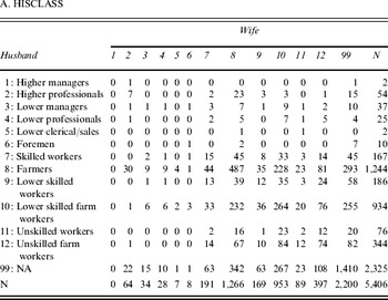
Table 1 (panel A) shows couples distributed by spouses' occupational origin according to the HISCLASS classification:Footnote 35 higher managers; higher professionals; lower managers; lower professionals, clerical and sales; lower clerical and sales; foremen; skilled workers; farmers; lower skilled workers; lower skilled farm workers; unskilled workers; and unskilled farm workers. Because the number of observations in some of the groups is very small, a seven-category classification is used in most of the analyses below, and its distribution is reported in panel B of Table 1.
Cross-classification of spousal social origin in the Scanian sample 1815–1895, all married couples


Source: The Scanian Demographic Database, Lund University.
The count in each cell is a function of both the matching process and the relative availability of partners, in other words the marginal distributions of the rows and columns in the table. If we assume that there is no structure in the matching process, the expected count in each cell will be given only by the marginal distributions. This situation is often referred to as the independence model. To test the presence of occupational homogamy in the population we estimate a model that includes a separate parameter for each diagonal cell in the table, that is for each cell where both the husband and his wife came from the same occupational origin:

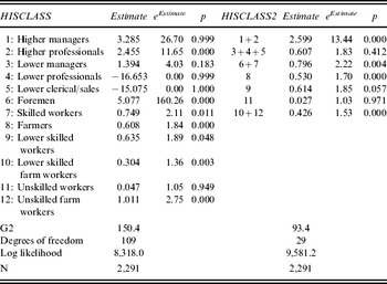
where f ij is the count in row i, column j; u is the grand mean; h i is the row parameter (husband's class origin); w j is the column parameter (wife's class origin); and d k is the diagonal parameter for cell k. The estimates of these diagonal parameters express the extent to which the count in the diagonal cells differs from what we would expect in a situation where matching was completely random. A positive value indicates that the (log) frequency in the diagonal cell is higher than expected, and thus that homogamy is more prevalent than could be expected from a random match, given the occupational structure on the marriage market. The exponents of the coefficients show the effects on the raw frequencies rather than on the log frequencies, and a value of 2.0 thus indicates that homogamy is twice as prevalent as in a random match. This kind of log-linear model has been widely used to analyse cross-classification count data of the kind available to us here,Footnote 36 social mobilityFootnote 37 and partner selection, both in historical and contemporary populations.Footnote 38
Table 2 displays the diagonal parameter estimates indicating the degree of homogamy in different occupational groups. It is quite clear that several of these groups show a high degree of homogamy (positive and statistically significant estimates), but some occupational groups did not marry homogamously to a higher extent than would be expected from a random match (negative or statistically non-significant estimates). The top segment of higher managers and professionals was the most homogamous, but it made up only about 1 per cent of the sample (see Table 1, panel B). Skilled workers (6+7), farmers (8), lower skilled workers (9), and farm workers (10+12) also show a high degree of homogamy. The lower middle class of managers, professionals, clerical and sales personnel (3+4+5) and the class of unskilled (non-farm) workers (11) do not show a significant tendency towards homogamy. In the case of lower managers, however, the estimated coefficient is of a comparable magnitude to several of the other classes showing homogamy, but is not statistically significant.
Log-linear estimates of homogamy parameters in the Scanian sample, all married couples 1814–1895

Source: See Table 1.
Thus we find a general tendency towards occupational homogamy. Occupational groups of higher social status and wealth were the most homogamous, probably because individuals and families strategically aimed at homogamous marriages as a way to maintain or increase income or wealth. The relatively large proportion of occupationally heterogamous unions between individuals from a higher professional (2) or farmer (8) background could be interpreted in a similar way (see Table 1); both occupational groups were wealthy and of high social status, and a marriage could fit the strategic aim described above even though the union was not occupationally homogamous. The tendency towards occupational homogamy among the least wealthy and among low-status occupations in rural areas (lower or unskilled workers, for example) was partly due to their exclusion from marriages with individuals of greater wealth and higher social status. The middle groups were heterogeneous with respect to wealth and social status, therefore more often entering occupationally heterogamous unions. In the next section we will deal in more detail with the attainment of occupational homogamy.
5. OCCUPATIONAL ATTAINMENT
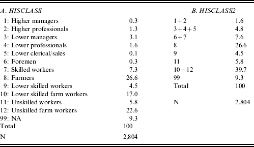
An important issue is whether partner choice affected occupational attainment, in other words whether marrying the ‘right’ partner had an impact on the occupation an individual ended up in. This is intimately connected to the wider issue of marriage strategies as a way to enhance one's social position, or at least avoid downward social mobility. We approach this issue by studying the impact of the occupational origins of the husband and his wife on the occupational attainment of the husband at age 45 (or at last observation between 35 and 45 for out-migrants). We have chosen this age because in most cases it was a time when individuals had advanced to their maximum lifetime occupational attainment, before retirement began and after the immediate post-marriage period when it was more likely that career advancement took place. We have also limited the analysis to husband's occupation because most married women lacked an occupation of their own, and did domestic work at home. Table 3 displays the occupational structure using HISCLASS for husbands at age 45. Clearly farmers (8) and farm workers (10+12) were the most numerous categories, at about 27 per cent and 40 per cent, respectively.
Occupational structure at husband's age 45 in the Scanian sample 1815–1895 (%)

Source: See Table 1.
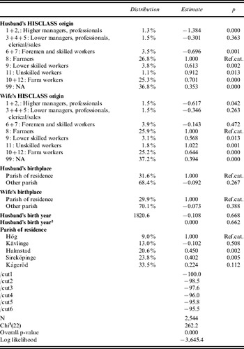
HISCLASS is clearly a hierarchical structure, even though it is somewhat unclear where in the hierarchy to put the farmers: whether they should be higher or lower than the skilled workers. Here we chose the original order where farmers are put between skilled workers and lower skilled workers. We model occupational attainment as an ordered logit model with achieved HISCLASS (seven categories) as the dependent variable.Footnote 39 We are primarily interested in how the occupational origins of the husband and his wife affected the occupational attainment at husband's age 45. We also control for their birthplaces, to capture the potential effects of social or kin networks which may have been stronger if a person was born in the parish of residence. The year of birth of the husband is included to control for changes over time, as is a square term to capture non-linearities in this effect (we also tried a specification with a period dummy, which did not change the results). Finally, we control for parish-specific differences by including parish of residence as a covariate. The distributions of these covariates and the model estimates are shown in Table 4.
Ordered logit estimates of husband's occupational attainment (HISCLASS) at age 45 in the Scanian sample, 1815–1895

Source: See Table 1.
The interpretation of the raw coefficients is not as straightforward as in the binary logit model. Assuming an underlying latent (unobserved) continuous dependent variable, the coefficients indicate the effect on this dependent variable. Thus, a positive value of the coefficient indicates that the covariate increases the likelihood of ending up in a lower-ranked occupational group (i.e. a higher value in HISCLASS). For example, relative to farmers' sons those from a lower skilled worker background (coefficient 0.613) are more likely to end up in a higher HISCLASS category (lower occupational status). Interpreted in this way it seems clear that the occupational origins of both the husband and his wife affected the occupational attainment of the household head. The higher the occupational status at birth, the higher the attained occupational status at age 45. The effects of origin seem somewhat stronger for the husband than for his wife in the higher classes. Neither the husband's nor his wife's birthplace seems to have mattered for occupational attainment, and the same is true for the husband's year of birth.
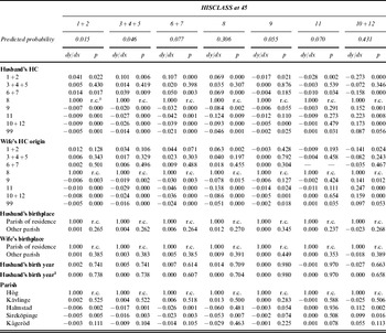
The results of the model estimations can also be used to predict the different occupational outcomes and to calculate the marginal effects of the covariates on these predicted outcomes (see Table 5). The marginal effects indicate the change in the probability of the outcome resulting from a one-unit change in the covariate. It should be noted that because the overall probabilities of the different outcomes vary a great deal, the marginal effects need to be related to these overall probabilities when interpreting the magnitude of the effects. For example, for the first outcome, where the overall probability is about 0.015, a marginal effect of 0.01 is quite sizeable, while for the last outcome, where the overall probability is 0.43, the same effect would be very small indeed.
Marginal effects from ordered logit estimations on predicted occupational attainment (HISCLASS) of husbands at age 45 in the Scanian sample, 1815–1895Footnote a

a Based on ordered logit estimates reported in Table 4. 1+2: Higher managers and professionals; 3+4+5: Lower managers, professionals, clerical and sales; 6+7: Foremen and skilled workers; 8: Farmers; 9: Lower skilled workers; 11: Unskilled workers; 10+12: Farm workers; 99: not available.
b r.c.=ref.cat.
Source: See Table 1.
The marginal effects show that the occupational origins of both the husband and his wife were important for occupational attainment. At least in the higher classes the effects of the wife's occupational origin were somewhat smaller than for the husband, but went in the same direction. In general the effects are also as expected. Looking at the upper part of the occupational distribution in the first column (HISCLASS 1+2), it is clear that those with a father in these occupations were considerably more likely to reach this level themselves. The marginal effects indicate, for example, that being the son of a higher manager or professional (1+2) increased the probability of reaching the top level by 4.1 percentage points compared to being a farmer's son, which is quite a lot because the overall probability of ending up in this class was only 1.5 per cent. Being married to a daughter from the same class also increased the probability of reaching this level, but only by 1.2 percentage points. At the other end of the occupational distribution (last column of Table 5) husbands from a worker background (HISCLASS 9–12) were also most likely to end up in the farm-worker class. It is also clear that the effects were quite powerful. Having a farm-worker origin increased the probability of becoming a farm worker by about 17 percentage points compared to being of farmer origin, which should be related to an overall probability of becoming a farm worker of 43 per cent. The comparable effects of the wife's origin were of a similar magnitude.
Taken together, these results show that the occupational origins of both the husband and his wife were highly important for occupational attainment. To reach the higher-status occupations, the husband's background was more important than that of his wife, but in the other cases their backgrounds were of similar importance. This indicates the importance not only of inherited factors in occupational attainment but also of finding the right partner.
6. OCCUPATIONAL MOBILITY
We now turn to the question of whether partner choice might have affected the likelihood of intergenerational occupational mobility either upwards or downwards. We have already seen that the social origins of both the husband and his wife affected the occupational attainment, but this does not necessarily imply that partner choice could be used as a way to climb the occupational ladder. Strong homogamy might, for example, have led to a strong tendency to non-mobility in occupational terms.
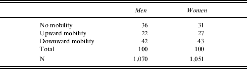
We study occupational mobility between generations by comparing the husband's occupation at age 45 with his and his wife's occupational backgrounds. Those ending up in an occupational group ranked higher than that into which they were born (based on the 12-category HISCLASS) are defined as having moved upwards, while those ending up in a group ranked lower are defined as having moved down. In order to allow all individuals to move in both directions we exclude HISCLASS 1+2 and 12 from the analysis.Footnote 40 Table 6 shows that roughly 20–30 per cent of the individuals experienced upward occupational mobility (22 per cent for men and 27 per cent for women), while over 40 per cent experienced downward mobility (42 per cent for men and 43 per cent for women). Thus, downward occupational mobility was considerably more likely than upward, which is fully in accordance with findings for other parts of Sweden in the same period.Footnote 41
Occupational mobility (%), men and women at husband's age 45 in the Scanian sample, 1815–1895Footnote a

a Occupational mobility is defined according to the 12-category HISCLASS. The sample includes only HISCLASS origins 3–11 in order to allow for all occupational groups to be mobile.
Source: See Table 1.
To study the impact of partner choice on occupational mobility we estimate a multinomial logit modelFootnote 42 distinguishing upward and downward mobility, in which non-mobility is the base outcome. As explanatory variables we include occupational background, marital union (homogamous, heterogamous upward, heterogamous downward),Footnote 43 place of birth, spouse's place of birth and parish of residence. We estimate separate models for men and women, but note that the occupation at age 45 is the same, namely the husband's occupation.
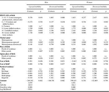
The results in Table 7 show clearly the importance of partner choice on both upward and downward mobility. Marrying a spouse of a higher occupational origin (heterogamy upwards) increased the likelihood of occupational mobility upwards. The effect went in the same direction for men and women, but it was considerably stronger for women. Similarly, marrying someone from a lower occupational background increased the likelihood of downward occupational mobility. In this case, too, the effect was present for both men and women but was slightly stronger for women. This shows not only that homogamy was a way to secure occupational status, as we saw in the previous section, but that heterogamy with someone from a higher-status background could actually improve the chances of climbing the occupational ladder. At the same time, heterogamy with someone from a lower-ranked background increased the risk of moving down and ending up in a lower occupational status than one's parents.
Multinomial logit estimates of occupational mobility, men and women at husband's age 45 in the Scanian sample, 1815–1895Footnote a

a Reference outcome is no occupational mobility. Occupational mobility is defined according to the 12-category HISCLASS. The sample includes only HISCLASS origins 3–11 in order to allow for all occupational groups to be mobile.
b r.c.=ref.cat.
c Based on 12-category HISCLASS.
Source: See Table 1.
The estimations in Table 7 also show that being born in another parish increased the likelihood of occupational mobility, both upwards and downwards. In other words, geographical ‘stayers’ were also ‘stayers’ in an occupational sense.
7. CONCLUSION
This article has shown that partner choice was closely connected to both occupational attainment and mobility in pre-industrial rural society. Even though the marriage pattern was characterized by a clear tendency towards occupational homogamy for most occupational classes, this should not hide the fact that many people, for various reasons, married heterogamously, both upwards and downwards. We have shown that the occupational backgrounds of both the husband and his wife were important for the occupational status attained by the family, as measured by the husband's occupation at age 45. Originating from a higher-status occupation also increased the likelihood of ending up in a higher-status occupation. Here, homogamy can be viewed as one important way of safeguarding the social (or occupational) reproduction of families. By marrying someone from a similar background, peasants, craftsmen and people of higher-status occupations tried to secure the social position of their children. Therefore, families planned strategically for homogamous unions that pooled economic resources, human capital and social networks in order to maintain or increase income, wealth and social status.
On the other hand, marrying heterogamously upwards could be used by people from lower-status origins as a strategy to enhance their prospects of intergenerational occupational mobility. We have been able to show that heterogamous marriages were significantly connected to occupational mobility in both directions. Controlling for own occupational background and geographical origin, marrying upwards increased the probability of occupational advancement, while marrying down increased the likelihood of downward occupational mobility. Because most occupational mobility in this area and period took place after marriage, or in conjunction with marriage, we are reasonably confident that partner choice was important for subsequent occupational attainment and mobility. It also seems to have been more important for women than for men.
These findings are consistent with several explanations linking partner choice with occupational attainment and mobility. One possibility is that it was the inherited assets of the higher-status spouse that contributed to the mobility of the other spouse. This can be seen most clearly in the case of peasants and craftsmen where the occupation relied upon the resources available (i.e. land, craft shop, tools and human capital for example). A second possible explanation is that the higher-status spouse enabled access to important networks, which in turn facilitated reaching higher occupations, for instance in the cases of higher-status occupations like managers and professionals. However, it may have been more difficult for a son-in-law to benefit from such networks than for a son, who gained access to them through the father. This is also clear in cases where occupations were more or less directly inherited. A third explanation is that individuals from a low-status background who managed to marry upwards and later climbed the occupational ladder may have had a higher ability than other individuals from a similar background, which made them more attractive on the marriage market and enabled them to advance occupationally. Similarly, some individuals in the higher-status occupations might have been less able and were forced to marry downwards, making it more difficult for them to maintain the same occupational status as their fathers. We cannot distinguish between these explanations, but it seems reasonable to expect a combination of them to explain the observed pattern.
ACKNOWLEDGEMENTS
An earlier version of this article was presented at the second symposium of COST Action 34 ‘The Transmission of Well-Being: Marriage Strategies and Inheritance Systems in Europe (17th–20th Centuries)’, University of Minho, Guimãres, Portugal, 25–28 April 2007. We are grateful to the participants for comments and suggestions. Martin Dribe acknowledges financial support from the Swedish Council for Working Life and Social Research (FAS).