1. Introduction

Flow stripes are visible in satellite images of most active and some inactive ice streams of the West Antarctic ice sheet. They usually have widths with in the range 0.1-10 ice thicknesses, and amplitudes of a few meters, and often extend for hundreds of kilometers (Reference Swithinbank and LucchittaSwithinbank and Lucchitta, 1986; Bindschadler, 1993; Reference Casassa and WhillansCasassa and Whillans, 1994). On the basis of previously established theories of glacier flow it is unclear flow surface features of this scale can be generated from the bed. in fact, the generation of features on this scale can be analyzed only with a theory which takes into account the effects of short-scale (on the order of one to ten ice thick-nesses) stress gradients on the flow, which is not done in most work on glacier flow. Furthermore, according to traditional kinematic-wave theory founded on prediction of motion from local thickness and slope (Reference NyeNye, 1960), stripes should decay by diffusion over a period o( a few days to weeks unless they are dynamically supported. Hence, neither the generation of the stripes nor their preservation over time can be explained with traditional theory of glacier flow.

Various hypotheses for the genesis of flow stripes have been suggested. Reference Merry and WhillansMerry and Whillans (1993) have summarized these attempts, and suggested that flow stripes are old shear margins. This is a possible explanation for the genesis of some of the observed flow stripes. On the other hand, a number of examples of the generation of flow stripes directly within active ice streams are known, one of which is shown in Figure 1.

Despite the lack of a satisfactory explanation for their origin and preservation over time, these stripes have been used to identify present and former ice streams and to infer changes in their flow dynamics and configuration (Reference MacAyeal, Bindschadler, Jezek and ShabtaieMacAyeal and others, 1988; Reference Hodge and DoppelhammerHodge and Doppelhammer, 1996). Our objective in this paper is to provide an explanation for both the origin and the longevity of flow stripes. We do this by applying an analytical theory of time-dependent linear flow in three dimensions, which has recently been developed. The details of the theoretical work, which does not relate specifically to flow stripes, will be given in a separate paper by G. H. Gudmundsson.

Fig. 1.

An example of the generation of a flow stripe within Ice Stream E, West Antarctica, from a Landsat Thematic Mapper sane. The meanflow direction is from the upper left to the lower right.

2 Theoretical Framework

We consider the problem of a Newtonian fluid that flows under the action of gravity, and we investigate the flow perturbations that result from two different types of boundary-conditions along the lower boundary: (1) bedrock undulations, and (2) spatial variations in resistance io basal sliding. Our purpose is to analyze the time-dependent evolution of the surface topography following the onset of the basal perturbations. We will limit the discussion mainly to conditions which resemble those of most active ice streams, where surface slopes are very small (about 0.1°) and the ratio of basal sliding to the internal deformational velocity is very large (<1000).

The mathematical analysis is based on perturbation methods. This sets a limit on the amplitudes of the basal perturbations. Hence, the thickness variations must be small compared to the mean ice thickness, and the variations in resistance to basal sliding must be small compared to the mean resistance. Apart from these restrictions, which presumably are met on most ice streams, the analytical solutions are quite general. They describe three-dimensional flow with evolving surface geometry, and although they are valid only for a linear medium, the viscosity may vary exponentially with depth. in particular, the solutions account rigorously for flow variations over short scales and the effects of both longitudinal and transverse stress gradients on the flow.

2.2. Geometry, field and boundary equations

A detailed description of the solution procedure will be given in the forthcoming paper by G. H. Gudmundsson. A short overview of the main steps leading to the analytical solutions is given here, with the aim of both clarifying the set of underlying assumptions and facilitating the understanding of the figures which follow.

A Cartesian coordinate system is used with the z axis normal to both the mean upper and lower boundaries. The slab has a mean inclination a, and the x and y axes are parallel and perpendicular to the mean slope, respectively. The z coordinates of the upper and the lower boundaries are given by the functions z_s(x, y) and z^b,(x, y). The field equations for incompressible, creep flow are

(1)

and

(2)

In the above equations, D is the rate-of-deformation tensor, v is the velocity vector, n is the viscosity, p is the pressure, f is the body force, and σ is the stress tensor. The rate-of-deformation tensor is defined as . Its components are the strain rates .

The viscosity can vary with depth according to

(3)

where is the viscosity at the surface, and ξ is a parameter which determines the rate of the vertical viscosity variation. For a positive ξ the viscosity at the surface is higher than at the base. An exponential viscosity profile accounts for an expected decrease of viscosity with depth in an approximate but reasonably realistic way. The temperatures in ice streams are expected to vary roughly linearly with depth (although the gradient may be stronger near the bed than near the surface). Assuming that the temperature effects on the viscosity of ice can be represented by ϒ, where Τ is the temperature, ϒ is a constant, and T_s is the surface temperature, a roughly linear temperature variation with depth leads to an approximately exponential viscosity variation.

The surface is not subjected to any stress, so that , for i = 1,2,3 and z = z_s(x, y), where m is a unit vector normal to the surface. The time-dependent evolution of the surface is governed by the kinematic boundary condition

(4)

where accumulation and ablation have been ignored.

Along the lower boundary neither the basal shear stress nor the basal sliding velocity is prescribed independently. Rather, the relation between them is specified through a sliding law

(5)

where u_b(x, y) is the basal sliding velocity. The function c(x, y) describes the spatial variation in resistance to basal sliding, and τ_b,(x,y) is the basal shear stress. The basal velocities are taken to be tangential to the lower boundary given by z_b(x, y).

2.4. Scalings

All variables having the dimension of length are scaled with the mean ice thickness h⁽⁰⁾. The stresses are scaled with the mean shear stress , the velocities with the mean deforma-tional velocity , and the time with the ratio of the mean ice thickness to the mean internal deformational velocity The kinematic boundary condition is invariant under this set of scalings, so that the evolution with time is the same in scaled as in dimensional variables.

Non-dimensional (or scaled) variables are denoted by upper-case letters. in non-dimensional form the mean ice thickness is equal to unity, the mean basal sliding velocity is the mean surface is Z_s = 0, the mean bed is Z_b = — 1, and the mean surface velocity is given by

(6)

where . The ratio of the mean sliding velocity to the mean deformational velocity, i.e. the slip ratio, is denoted by Ω. Note that as the rate of the vertical viscosity variation changes, the sliding velocity remains constant, while the internal deformational velocity varies. Also note that the ratio of the surface viscosity to the basal viscosity is given by .

In non-dimensional variables the sliding law has the form where U_b is the sliding velocity, and ΔC(X,Y) is the C-perturbation, which must be small compared to unity. The bedrock perturbation is ΔΖ(Χ, Y) and it must also be small compared to unity (i.e. the mean ice thickness). All field deviations from their mean values (i.e. anomalous fields) depend linearly on ΔC(X, Y) and ΔZ(X, Y).

2.5. Analytical solutions

As examples of the analytical solutions we give the Fourier transforms of the time-dependent transfer functions for the Z- and C-perturbations.These analytical solutions are valid for a constant viscosity profile with depth, i.e. Ξ = 0. The transfer functions describe the effect of the basal perturbations on the surface topography. Multiplication of the transfer functions with the Fourier transform of the basal perturbations gives the corresponding surface perturbations.

The transfer function describing the effect of a Z-pertur-bation on the surface topography is given by

(7)

and the transfer of a C-perturbation to the surface is given by

(8)

where i, is the imaginary unit, and the following abbreviations have been used:

(9)

(10)

(11)

(12)

(13)

and

(14)

The two time-scales t _d and t _p, referred to as the diffusion time-scale and the propagation time-scale, respectively, are given by

(15)

In the above equations, k_x and k_y are the longitudinal and transverse wavenumbers, respectively, and k is defined as [k_x ² + k_y ²)^1/2. These wavenumbers are dimensionless, although written in lower case. A value of k_x = 1 corresponds to a longitudinal undulation having a wavelength of 2π times the mean ice thickness. The expressions for the time-scales t_p and t _d are also without dimensions. Dimensional times are obtained by multiplying t _d and t _p with the ratio .

3 Examples For Flow Over Basal Perturbations At High Sliding Velocities

Figure 2 shows the response of the surface to flow over both a Z- and a C-perturbation at the base. Both basal perturbations are of Gaussian shape given by the function . For convenience the amplitudes of both basal perturbations were set to unity. Hence, for a basal bedrock undulation with the same shape but a different amplitude of, for example, 10% of the mean ice thickness, the surface undulations will be 10% of what is shown in figure 2a. The Z-perturbation corresponds to a bedrock bump protruding into the base of the ice stream, and the C-perturbation to an area with enhanced resistance to basal sliding (negative ΔC) with respect to the surrounding area. C-perturbations are important for the dynamics and the existence of ice streams. The ice-stream margins correspond to sharp transverse variations in slip resistance (Reference BentleyBentley, 1987; Raymond, 1996), and variations in slip resistance within ice streams may be the cause of areas of rougher surface relief (MacAyeal, 1992; Bindschadlcr and others, 1996).

The basal perturbations are turned on at time t = 0, and the situation at t = 2 is shown. Typical surface velocities for active Siple Coast ice streams are some 500 m a⁻¹, and ice thicknesses are around 1000 m. Then, accounting for the time-scaling used in this figure, which is (and not as above), a time interval of 2 corresponds to about 4 years. The values of the other input parameters are given in the figure caption.

The slip ratio Ω was estimated by calculating the deformational velocity for a linear temperature profile with surface temperatures at -25°C and basal temperatures at the melting point, for an ice thickness of about 1000 m and surface slope of 0.1° using the Smith-Morland relation between the rate factor and temperature (Reference Smith and MorlandSmith and Morland, 1981). Depending on the exact numerical values used, a value for Ω in the range from a few thousand to a few tens of thousands results. A standard value of Ω = 10 000 has been used for the figures shown.

Fig. 2.

Map plane view of surface undulations caused by Gaussian-shaped Ζ-perturbations (a) and C-perturbations (b) at the base (white contour lines). The unit of the X and Y axes is one mean ice thickness. The shape of the basal perturbation is shown with black-colored and dash-dotted contour lines. The mean surface elevation is zero and the mean ice thickness is equal to unity. Higher-than-average surface elevations are plotted with solid contour lines, and lower-than-average surface elevations with dashed lines. The mean flow direction is from left to right. The basalflow perturbations are turned on at time t = 0, and the surface response at time t = 2 is shown. This dimensionless time interval can be interpreted as dimensional time by multiplication with the ratio of mean ice thickness to mean surface velocity (). in one time unit the ice travels a distance ofone mean ice thickness. Other relevant parameters are: σ_x = σ_y = 2 (the longitudinal and transverse widths of the basal perturbations), α= 0.1° (mean surface slope), Ω = 10000 (slip ratio), and = 0 (viscosity variation with depth). The amplitudes of the Z-and C-perturbations are equal to +1 and -1, respectively.

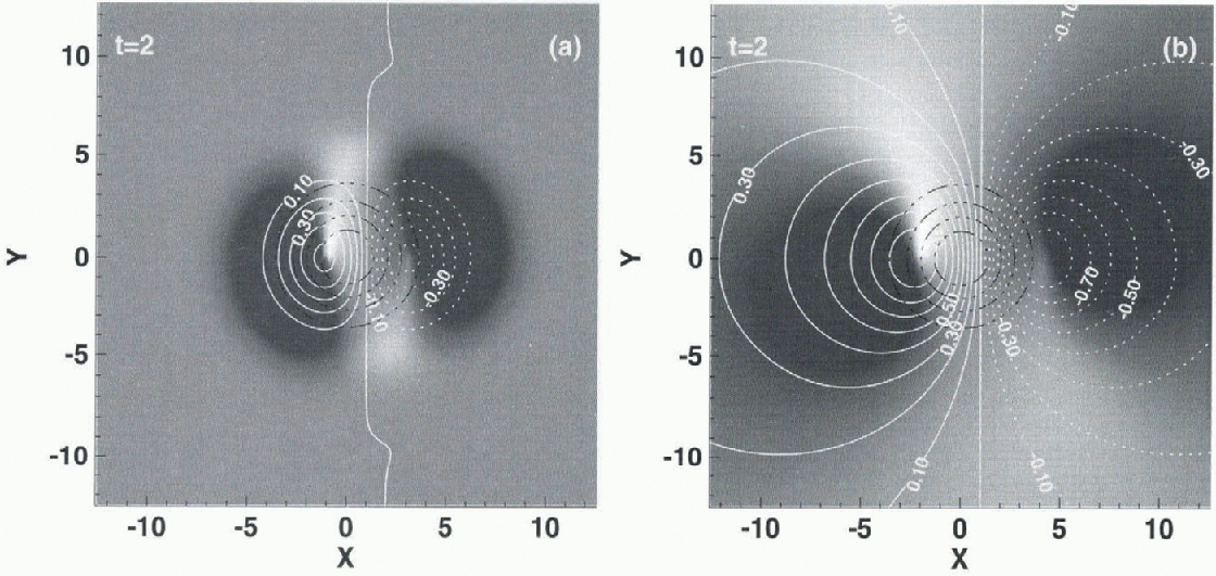
Figure 2 shows flow the ice is piled up at the upstream sides, and a surface depression is formed on the downstream sides, of both the Z- and C-perturbations as the ice stream flows over and around them. The spatial scale of the resulting surface undulations is very different. The C-perturbation has a much broader effect on the surface than the Z-perturbation. The C-perturbation response is not localized, in the sense that it is not limited to the width of the applied basal perturbation. This C-pcrturbation response was found by Raymond (1996) in connection with the effect of transverse variations in basal slip-resistance. Note that only the size, not the shape, of the surface perturbation depends on the amplitude of the applied basal perturbations.

The situations at t = 80 and are depicted in Figure 3. The originally formed depressions seen in Figure 2 have been advected downstream, and at the same time their amplitudes have become smaller. Interestingly, the depressions have traced out “tracks” in the surface of the ice. The surface rise is still at essentially the same spot as it was at t = 2, or just slightly upstream of the bedrock perturbation. As time advances further, the amplitudes of the originally-formed surface depressions (Fig. 2) continue to decrease, and in the steady-stale limit these depressions have completely disappeared (fig. 3c and d). What remains is the surface rise and a flow feature which strongly resembles the flow stripes seen on active ice streams (cf. figs 1 and 3c). The steady-state surface rise could be referred to as the “head” of the flow stripe, and this type of flow-stripe genesis as a “base-generated” flow stripe. A (steady-state) base-generated flow stripe always has a head, and the sign of the surface amplitude of the head is different from that of the flow stripe.

It is important to realize that because the amplitudes of the surface undulations depend linearly on the amplitudes of the basal perturbations, a bedrock depression and a “slippery spot” will give rise to a flow stripe which rises above the surrounding ice. Also note that a 1 % surface amplitude, for example, can be generated by only 0.75% C-perturbation (fig. 3d).

Reducing the transverse width of the basal perturbations gives narrower flow stripes which decay over longer distances. Flow stripes having widths considerably smaller than the ones shown in Figure 3 (less than h⁽⁰⁾ can also be generated from the bed.

The flow stripe is continuously regenerated through ad-vection of ice. Hence, as the steady-state solution demonstrates (fig. 3c and d), the flow stripe docs not decay with time. Flow stripes generated in the way depicted in Figure 3 never decay as long as the basal perturbation persists and the ice stream continues to flow. There is, therefore, no upper limit to the lifetime of flow stripes, only to their length. This picture differs from the conception of flow stripes as being old, inactive shear margins, in which case flow stripes must have a finite lifetime.

The genesis of the flow stripes follows from the fact that basal perturbations can, if they have the right spatial dimensions, be transferred rather easily to the surface. The longevity is related to the long diffusion time at short spatial scales. Both the spatial and the temporal transfer characteristics predicted by the first-order three-dimensional short-scale theory differ strongly from predictions based on the assumption that the direction and the magnitude of ice flow is at every location dependent only on the local ice thickness and the local surface slope. Technically, this difference follows from the different treatment of the terms in the momentum equations describing horizontal stress gradients. Ignoring horizontal stress gradients leads to flow fields which depend only on the local thickness and slope. Including horizontal stress gradients, on the other hand, means that stress disturbances can be transmitted over some distance l, referred to as the coupling length. As a result, the ice flow at every location does not depend only on the local slope and thickness, but becomes affected by the whole stress regime with in the distance l The flow of fea-tures having horizontal spatial scales smaller than coupling length l can be described correctly, therefore, only if stress gradients are rigorously accounted for. As shown below, the coupling length l on ice streams is much larger than the typical horizontal spatial dimensions of flow stripes. Hence, the inclusion of stress gradients is crucial for a correct theoretical description of their flow characteristics.

Fig. 3.

Surface undulations caused by Gaussian-shaped basal Z-perturbations (a and c) and C-perturbations (b and d) for t = 80 and . All other parameters are the same as in Figure 2. Note thai the contour interval is not constant. (For the surface rise in (a) and (c) the contour interval is 0.2 in units of mean ice thicknesses.) (e) gives the surface amplitudes seen in (a)-(d) along the line Y = 0 as afunction of X.

4. Transfer Characteristics

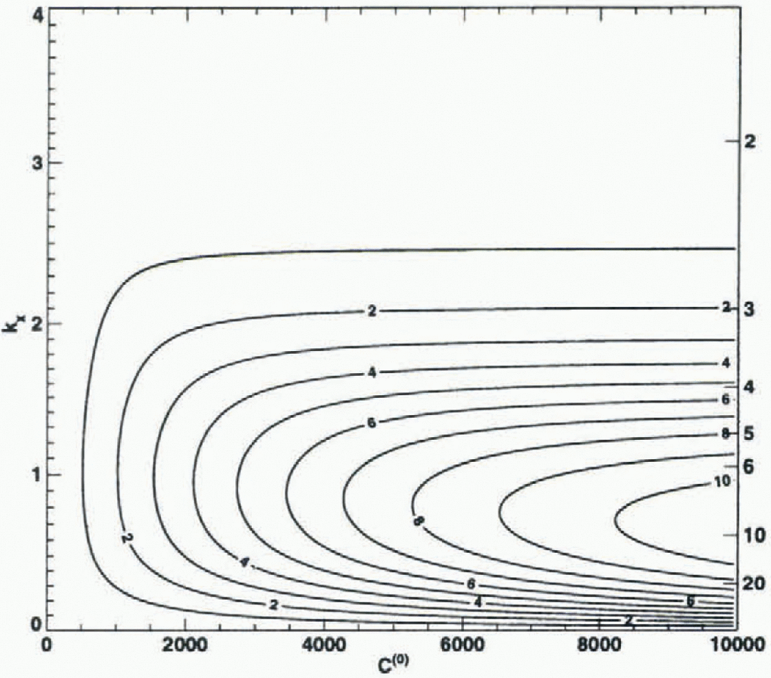
The transfer functions T_zz(t;k_x,k_y) and T_zc(t;, k_x, k_y) (Equations (7) and (8)) give the relation between the applied Z- and C-perturbations and the resulting surface topography. Figure 4 shows the magnitude of the steady-state () transfer function Τ_zz as a function of the longitudinal wavenumber and the sliding-law parameter , for k_y = 1 and Ξ = 5. A value close to unity represents an almost perfect transmission of basal bedrock undulations to the surface, and a value of zero no transmission. A conspicuous aspect of the figure is the selective transmission of basal undulations to the surface at high basal sliding velocities. The ice acts as a relatively narrow band-pass filter. Only a selected range of longitudinal wavelengths is transmitted to the surface without substantial attenuation. As an example: for C⁽⁰⁾ = 5000, which corresponds to Ω ≈ 15000 (see Equation (6)), about 70% of the amplitude of a sinusoidal bedrock undulation with is transmitted to the surface. The narrowness of this band-pass filter increases with increasing C⁽⁰⁾, and at the same time an ever larger fraction of the basal amplitudes is transmitted. Hence, bedrock undulations having wavelengths 6-10 times the mean ice thickness are very effectively transmitted to the surface of ice streams. For ice sheets, ice caps and glaciers, where the slip ratio Ω typically ranges from 0 to about 100 at the most, this band-pass effect is of comparatively little importance.

Fig. 4.

The steady-state transfer function T_zz describing the transfer of bedrock undulations to the glacier surface as a function of the sliding-law parameter and the wavenumber . The transfer function gives the ratio of the amplitude ofa sinusoidal surface undulation to the amplitude of a sinusoidal bedrock undulation having the same wavelength. With increasing C⁽⁰⁾ the slip ratio (ratio of mean basal sliding velocity to mean ice-defortna-tional velocity) increases (Equation (6)). in ice streams, C⁽⁰⁾ may well be somewhere with in the range 5000-10 000, whereas for most glaciers C⁽⁰⁾ is less than 10. From the shape of the transfer function, it follows that in ice streams longitudinal bedrock undulations having ivavelengths of 5-10 mean ice thicknesses are transferred to the surface with only a modest amplitude attenuation.

The band-pass effect can be understood in rather simple terms. The amplitude of the (non-dimensional) anomalous flow is proportional to the slope α/λ of the bedrock undulations, that is, to the rate of the thickness variations and not to the thickness changes themselves. Hence, for a given a the maximum amplitude of the anomalous flow decreases as λ increases. On the other hand, the vertical extent of the anomalous flow scales with λ. Thus, for small wavelengths (λ ≤ 1) the induced flow disturbances are large, but limited to the lowermost layers and therefore without appreciable effect on the surface geometry. With increasing λ, however, the anomalous flow has progressively more effect on the surface geometry, but at the same time the overall amplitudes of the anomalous flow decrease. Since for the amplitudes of the induced flow disturbances go to zero, it follows that there will be some intermediate wavelength for which the transfer reaches a maximum.

In Figure 5, the T_zc transfer function is shown for the same set of values as used in Figure 4. Note that because the cause, i.e. the C-pcrturbation, and the effect, i.e. the surface undulation, are different physical quantities, no simple meaning can be given to the magnitude of the filter, except that higher values mean larger resulting surface undulations. The figure shows very much the same filter characteristics as seen in Figure 4. in particular, the band-pass effect is equally important for the C- as for the Z-perturbations. A close inspection of both figures, however, shows that the maximum of the transfer function T_zc is, for each fixed value of C⁽⁰⁾ displaced towards somewhat longer wavelengths as compared to T_zz-

5 Time-Scales

The time-dependent internal deformation of glaciers is governed by the two time-scales t_d and t _p having to do with diffusion and propagation of disturbances. The dependency of the diffusion and the propagation time-scales on the ratio of the longitudinal wavelength to mean ice thickness was first investigated by Reference Landon and RaymondLandon and Raymond (1978) in a numerical model, and later analytically byjóhanncsson (1992). in the long-wavelength limit, where longitudinal stress gradients are not important, the traditional kinematic-wave theory can be used to calculate these time-scales, and it predicts decay times of a few days to weeks and a phase velocity of a few times the surface velocity. The time-scales calculated from the short-scale flow theory (see Equation (15)) give the known long-wavelength limits, which originally were derived using entirely different methods (Nyc, 1960), for k_x —> 0 and k_y = 0. On short spatial scales, however, the diffusion time ij is much longer than predicted from a linear extrapolation of the long-wavelength limit to short spatial scales. On short scales the phase velocity equals the mean surface velocity as expected, whereas the traditional theory predicts a phase velocity of twice the surface velocity (for a Newtonian medium).

Fig. 5.

The steady-state transfer function T_zc describing the effect of spatial variations in resistance to basal sliding on the surface geometry for ky = 1, a = 0.1° and .

Fig. 6.

The diffusion/build-up time-scale t _d as a Junction of the longitudinal wavelength . The thin dash-dotted lines give the long-wavelength limit, which is (in units ). The solid and the dotted tines were calculated for and respectively. The dotted lines exemplify flow the finite transverse extent of the perturbations can affect their diffusion time, so that the long-wavelength limit is not even reached as . The surface slope is a = 0.1° and there is no temperature variation with depth ().

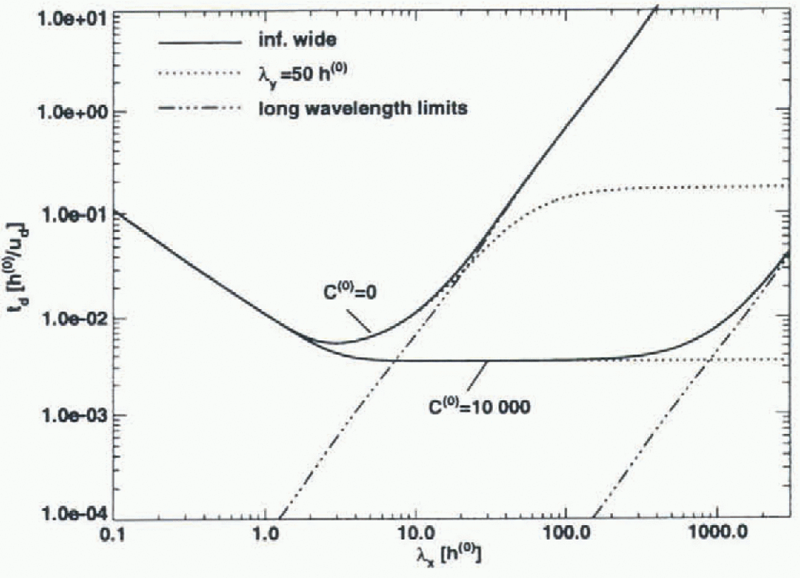
The diffusion time t _d is plotted in Figure 6 as a function of the wavelength λ where . Note that the longitudinal and transverse wavenumbers k_x and k_y affect t_d only through k. The alignment of a surface undulation with respect to the flow direction has therefore no effect on the diffusion rale, which is a physically reasonable result. Three different spatial scales (short, intermediate, long) can be identified in Figure 6. On short scales . This short-wavelenglh limit corresponds to a viscous relaxation over a half-space. in the long-wavelength limit , which is a result originally obtained by Nye (1960). in the intermediate range t_d does not depend on λ; an expected result for a viscous relaxation over a layer. The wavelengths in the inlermediate range are long enough for the finite ice thickness to have a noticeable effect on the transient evolution, and at the same time these wavelengths are shorter than the coupling length over which stress gradients are transmit ted. The transition from the intermediate spatial scale to the long-wavclcngth limit marks the boundary between the regions of “stress-gradient-affected” flow and “stress-gradient-independent” flow. For C⁽⁰⁾ = 10 000 this transition takes place at the staggering value of a few hundred mean ice thicknesses, which effectively means that ice streams are significantly affected by stress gradients at all relevant spatial scales. Figure 6 gives a diffusion time of several hundred years for C⁽⁰⁾ = 10000, and an iee-thickness-to-surface-velocity ratio of 2 years (a typical ratio for the Siple Coast ice streams). Diffusion times on this order are compatible with the observation that surface features on ice streams can persist for prolonged time periods.

Not only basal perturbations may give rise to flow stripes. Flow stripes can, for example, often be traced back to the confluence of two ice streams (Swithinbank and Luc-chitta, 1986; Casassa and others, 1991), and a possible explanation for the genesis of these flow stripes has been offered (Reference Vornberger and WhillansVornberger and Whillans, 1986). From the long diffusion times (several hundred years) on short spatial scales and the high surface velocities of ice streams, it follows that every sufficiently localized surface undulation — generated in one way or another by the mechanics of glacier flow — is stretched out in the downstream direction over considerable distances, leading to the formation of a flow stripe. That surface features on ice streams could possibly be elongated in this fashion in the downstream direction was anticipated by Hodge and Doppel hammer (1996).

6. Conclusion

A flow stripe is formed whenever ice flows over a basal perturbation having a spatial extent comparable to the ice thickness at high basal sliding velocities. No special theological properties of the ice are needed for this purpose. Non-linearities in the flow law must be expected to affect somewhat the quantitative results, but not to change the overall picture. Neither the genesis nor the longevity of flow-stripes poses fundamental problems, and both can be understood to be straightforward consequences of the properties of viscous creep flow.

Previous theoretical work on glacier flow lias not accounted for the effects of longitudinal coupling over short spatial scales and for tin- three-dimensionality of glacier flow to the extent done here. At short spatial scales stress gradients affect drastically both the transform characteristics of basal perturbations through the ice towards the surface, and the magnitudes of both the diffusion and propagation time-scales. A rapidly sliding ice stream is exceedingly “transparent” to bedrock undulations having wavelengths which are a few times the mean ice thickness, and bedrock undulations on this spatial scale are easily transferred to the surface. The diffusion time-scale is also very long at these wavelengths, or on the order of 100 years for a linear medium.