2 Preliminaries

We denote the sets of natural numbers, positive integers, and real numbers by $\mathbb {N}$ , $\mathbb {Z}^+$ , and $\mathbb {R}$ , respectively. We denote the powerset of a set X by $\wp (X)$ . Given a set X and a binary operation symbol $\cdot $ , we denote by $(X^*,\cdot ,1)$ the free commutative monoid generated by X with unit $1$ . A substitution on X is a monoid homomorphism ${\boldsymbol {\sigma }}:X^*\to X^*$ ; substitutions are determined by their restriction to X. For $x\in X^*$ , we write $x^n$ to denote $1$ , if $n=0$ , and the term $x\cdot \cdots \cdot x$ consisting of n copies of x for $n>0$ . For subsets $A,B$ of X, we define $A\cdot B=\{a\cdot b: a\in A,b\in B\}$ , and if $a\in X$ then $a\cdot B=\{a\}\cdot B$ .

Let $\mathcal {L}$ be an algebraic language, i.e., containing no relational symbols. Given a set of variables X, $T(X)$ denotes the set of terms over X and $\mathcal {L}$ and $\textbf{T}(X)$ the absolutely free algebra of terms. A quasiequation is (the universal closure of) a formula of the form

(1) $$ \begin{align}s_1=t_1~ \&\cdots\&~ s_n=t_n \implies s_0=t_0, \end{align} $$

where $s_0,t_0,\ldots ,s_n,t_n\in T(X)$ are terms and $n \in \mathbb {N}$ . If $n=0$ then the left-hand side is empty and we obtain an equation.

For a class of algebras $\mathcal {K}$ in the language $\mathcal {L}$ , we say that (1) holds in $\mathcal {K}$ (i.e., $\mathcal {K}\models $ (1)) if for every algebra $\textbf{A}\in \mathcal {K}$ and homomorphism $h:\textbf{T}(X)\to \textbf{A},$

$$ \begin{align*}(\forall i\in \{1,\ldots,n\}) (\textbf{A},h\models s_i=t_i ) \implies \textbf{A},h\models s_0=t_0.\end{align*} $$

Here $\textbf{A}, h \models s=t$ means $h(s)=_{\textbf{A}}h(t)$ .

A presentation is a pair $\langle X,E\rangle $ where X is a set of generators and E is a set of equations over $T(X)$ . A presentation $\langle X,E\rangle $ is said to be finite iff both X and E are finite. We denote the conjunction of equations in E by $\&E$ . For a variety of algebras $\mathcal {V}$ in the language $\mathcal {L}$ , we say $\mathcal {V}$ has an undecidable word problem if there exists a finite presentation $\langle X,E\rangle $ such that there is no algorithm that on input $s,t\in T(X)$ decides whether the quasiequation

(2) $$ \begin{align}\& E \implies s=t \end{align} $$

holds in $\mathcal {V}$ . Note that if $\mathcal {V}$ has undecidable word problem then its quasiequational and universal theories are undecidable as well. The word problem is also referred to as the local word problem and the quasiequational theory as the global word problem, making explicit that in the former the antecedent of the quasiequations is fixed while in the latter it is unrestricted.

In the following the proofs of the undecidability of the word problem will rely on the fact that residuated lattices have a $\{\vee , \cdot , 1\}$ -reduct, and therefore the undecidability results apply to all reducts that contain it.

3 Counter machines

For proving undecidability we use a type of abstract machine known as an And-branching k-Counter Machine (k-ACM), introduced in [Reference Lothaire11], as they have an undecidable halting problem. A k-ACM is a tuple ${\texttt{M}}=(\texttt{R}_k, {\texttt{Q}},{\texttt{P}}, q_f)$ representing a type of parallel-computing counter machine, where

• • $\texttt{R}_k:=\{\texttt{r}_1,\ldots ,\texttt{r}_k\}$ is a set of k registers, each able to store a nonnegative integer (representing the number of tokens in that register),

• • ${\texttt{Q}}$ is a finite set of states with a designated final state $q_f$ , and

• • ${\texttt{P}}$ is a finite set of instructions (to be formalized below) that indicate whether to, given a certain state of the machine, increment a register or decrement a nonzero register, as well as a “branching” instruction known as forking, with no instruction applicable to the state $q_f$ .

A configuration ${\texttt{C}}$ of a k-ACM is a tuple consisting of a single state and, for each register, a nonnegative integer indicating the contents of that register. We can imagine a configuration being a box labeled by a state and containing tokens each labelled by an element of the set $\texttt{R}_k$ . In essence, a configuration is specified by the state label and the multiset of register labels of the tokens. Since the order of the symbols is irrelevant, we represent a configuration ${\texttt{C}}$ as a term in the free commutative monoid generated by ${\texttt{Q}}\cup \texttt{R}_k$ , and canonically arranged as

$$ \begin{align*} q\texttt{r}_1^{n_1} \texttt{r}_2^{n_2}\cdots \texttt{r}_k^{n_k}, \end{align*} $$

where $q\in {\texttt{Q}}$ is the state of the configuration and $n_i$ is the number stored in the register $\texttt{r}_i$ , for each $i=1,...,k$ ; if $n_i=0$ , we say the register $\texttt{r}_i$ is empty. Since ${\texttt{C}}$ contains precisely one state, we may define the set of configurations by $\texttt{Conf}(\texttt{M}) := {\texttt{Q}}\cdot \texttt{R}_k^*$ .

The instructions of a k-ACM replace a single configuration by a new configuration (via increment and decrement), or by two configurations (via forking). An increment instruction can be understood as “if a box is labeled by state q, add one register- $\texttt{r}_i$ token and relabel the box with state $q'$ ,” decrement as “if a box is labeled by state q, and $\texttt{r}_i$ is not empty, remove one register- $\texttt{r}_i$ token and relabel the box with state $q'$ ,” and forking as “if a box is labeled by state q, duplicate the box and its contents, resulting in two boxes relabeled by $q'$ and $q"$ , respectively.” As a consequence of the forking instruction, the machine can be operating on multiple configurations, i.e., branches, in parallel and is inherently nondeterministic. The status of a machine at a given moment in a computation, called an instantaneous description (ID), is represented by the configurations that are present. Formally, an ID is an element

$$ \begin{align*} {\texttt{C}}_1\vee\cdots\vee {\texttt{C}}_m, \end{align*} $$

of the free commutative semigroup $\texttt{ID}(\texttt{M})$ generated by $\texttt{Conf}(\texttt{M})$ ; we denote the associated binary operation by $\vee $ .

In this way, we view $\texttt{ID}(\texttt{M})$ as a subset of the commutative semiring ${\textbf{A}_{\texttt{M}}}=(A_{\texttt{M}}, \vee , \cdot , \bot , 1)$ generated by $\texttt{R}_k\cup {\texttt{Q}}$ , where

• • $(A_{\texttt{M}},\vee ,\bot )$ is a commutative monoid with additive identity $\bot $ ,

• • $(A_{\texttt{M}},\cdot ,1)$ is a commutative monoid with multiplicative identity 1, and

• • multiplication distributes over join.

Even though $\vee $ in $\textbf{A}_{\texttt{M}}$ is not defined to be idempotent, we will consider homomorphisms from $\textbf{A}_{\texttt{M}}$ that will map $\vee $ to a semilattice operation and for our applications it would not hurt to define $\vee $ to be idempotent. However, the non-idempotent status of ID’s matches better the intuition of computation and this is the reason for our choice.

Since multiplication fully distributes over $\vee $ in $\textbf{A}_{\texttt{M}}$ , each element of $A_{\texttt{M}}$ can be written as a finite join $\bigvee _{i\in I} m_i$ , where I is a finite (possibly empty) set, of monoid terms $m_i \in ({\texttt{Q}} \cup \texttt{R}_k)^*$ , for all $i \in I$ ; recall that the join of the empty set is the bottom element ( $\bot =\bigvee \emptyset $ ). As usual, each element of $\textbf{A}_{\texttt{M}}$ , which is the equivalence class $[t]$ of a term t in the absolutely free algebra over $\{\vee , \cdot , 1\}$ and ${\texttt{Q}} \cup \texttt{R}_k$ , will be identified with the term t itself, when no confusion arises.

Formally, an instruction p of a k-ACM is an expression of the form $q\leq q'\texttt{r}_i$ , $q\texttt{r}_i \leq q'$ , or $q\leq q'\vee q"$ , where $q, q', q" \in {\texttt{Q}}$ and $\texttt{r}_i \in \texttt{R}_k$ , representing increment $\texttt{r}_i$ , decrement $\texttt{r}_i$ , and fork, respectively. We will often write $p:{\texttt{C}}\leq {\texttt{u}}$ to indicate the instruction p is given by ${\texttt{C}}\leq {\texttt{u}}$ , where ${\texttt{C}} \in \texttt{Conf}(\texttt{M})$ and ${\texttt{u}} \in \texttt{ID}(\texttt{M})$ . For a state $q\in \texttt{Q}$ , we say p is a q-instruction if $p:qx\leq \texttt{u}$ for some $x\in \texttt{R}_k^*$ . Note that a machine $\texttt{M}$ with final state $q_f$ contains no $q_f$ -instructions by definition.

The computation relation $\leq $ for the machine ${\texttt{M}}=(\texttt{R}_K,{\texttt{Q}},{\texttt{P}},q_f)$ is defined to be the smallest ${\{\cdot ,\vee \}}$ -compatible preorder containing ${\texttt{P}}$ , and will be denoted by $\leq _{\texttt{M}}$ . For a given instruction $p: {\texttt{C}}\leq {\texttt{u}}$ , it will be useful to define the relation $\leq ^p$ to be the closure of p under the inference rules

for all $v,w,x,t\in A_{\texttt{M}}$ (in that order, without loss of generality, due to the distributivity of $\cdot $ over $\vee $ ). Consequently, $v\leq ^p w$ if and only if $v={\texttt{C}}x\vee t$ and $w=\texttt{u} x\vee t$ , for some $x, t \in A_{\texttt{M}}$ ; these equalities are understood inside $ A_{\texttt{M}}$ , so the terms $v$ and ${\texttt{C}}x\vee t$ need not be identical. We therefore conclude that if $v\leq ^p w$ , then $v\in \texttt{ID}(\texttt{M})$ if and only if $w\in \texttt{ID}(\texttt{M})$ .

It is easily verified that $\leq _{\texttt{M}}$ is equivalent to the smallest preorder generated by $\bigcup \{\leq ^p: p\in {\texttt{P}}\}$ . Therefore, if $s\leq _{\texttt{M}} t$ , then there exist $n \in \mathbb {N}$ , a sequence of $A_{\texttt{M}}$ -terms $t_0, \ldots , t_n$ and a sequence of instructions $p_1, \ldots , p_n$ from ${\texttt{P}}$ , collectively called a computation in ${\texttt{M}}$ of length n witnessing $s\leq _{\texttt{M}} t$ , such that

$$ \begin{align*}s_0=_{\textbf{A}_{\texttt{M}}}t_0 \leq^{p_1} t_1 \leq^{p_2}\cdots \leq^{p_n} t_n=_{\textbf{A}_{\texttt{M}}} t.\end{align*} $$

Clearly, if there is a computation witnessing $s\leq _{\texttt{M}} t$ , then there is a computation of minimal length, the value of which we simply call the computation length. The following result is an easy consequence of the definitions.

An ID consisting entirely of configurations labeled by the state $q_f$ with all registers empty is called a final ID and we denote the set of final ID’s by ${\texttt{Fin}}({\texttt{M}}):= \{ \bigvee _{i=1}^n q_f: n\geq 1\}$ . Our choice to not assume the idempotency of $\vee $ in $\textbf{A}_{\texttt{M}}$ explains the necessity of treating $ \bigvee _{i=1}^n q_f$ as a final ID. We say that a term $t\in A_{\texttt{M}}$ is accepted by ${\texttt{M}}$ if there exists ${\texttt{u}}_f\in {\texttt{Fin}}({\texttt{M}})$ such that $t\leq _{\texttt{M}} {\texttt{u}}_f$ , and we define the set of accepted terms to be ${\mathrm{Acc}}({\texttt{M}}):=\{t\in A_{\texttt{M}}: \exists {\texttt{u}}_f\in {\texttt{Fin}}({\texttt{M}}),~t\leq _{\texttt{M}} {\texttt{u}}_f \}$ .

Example 3.3. Consider the $1$ -ACM ${\texttt{M}}_{\mathrm {even}}= (\texttt{R}_1,{\texttt{Q}}_{\mathrm {even}},{\texttt{P}}_{\mathrm {even}},q_f)$ , where ${\texttt{Q}}_{\mathrm {even}}=\{q_0,q_1,q_f\}$ and ${\texttt{P}}_{\mathrm {even}}=\{ p_0,p_1,p_f\}$ is given by

$$ \begin{align*}\begin{array}{ l c r c l} p_0 &:& q_0 \texttt{r}_1& \leq & q_1, \\ p_1 &:& q_1 \texttt{r}_1& \leq & q_0, \\ p_f &:& q_0 & \leq & q_f\vee q_f. \end{array}\end{align*} $$

For example, $q_0\texttt{r}_1^2\leq ^{p_0} q_1\texttt{r}_1 \leq ^{p_1} q_0 \leq ^{p_f} q_f \vee q_f$ is a computation showing that $q_0\texttt{r}_1^2$ is accepted. On the other hand $q_0\texttt{r}_1 \leq ^{p_0} q_1$ and $q_0\texttt{r}_1 \leq ^{p_f} (q_f \vee q_f)\texttt{r}_1=q_f\texttt{r}_1 \vee q_f\texttt{r}_1$ are the only maximal computations starting with $q_0\texttt{r}_1$ and none of them ends in a final configuration, so $q_0\texttt{r}_1$ is not accepted. In general, it is easy to see that $q_0\texttt{r}_1^n\in {\mathrm {Acc}}({\texttt{M}}_{\mathrm {even}})$ if and only if n is even.

Lemma 3.4 shows that in a computation witnessing the acceptance of an ID all configurations are ID’s and therefore for those cases the inference rule $[\cdot ]$ could have been restricted to $x \in \texttt{R}_k^*$ .

4 Machines and residuated frames

As a demonstration of our general technique, we will use counter machines and residuated frames to show that any variety between $\mathsf {CRL} $ and $\mathsf {RL} $ has an undecidable word problem.

Let $\texttt{M}=(\texttt{R}_k,\texttt{Q},\texttt{P},q_f)$ be an ACM. For each $u\in \texttt{ID}(\texttt{M})$ , formally viewed as an $\{\vee ,\cdot ,1\}$ -term in $\textbf{T}(\texttt{R}_k\cup \texttt{Q})$ , we define the quasiequation $\mathrm {acc}_{\texttt{M}}(u)$ to be

where $q_f$ is the final state of ${\texttt{M}}$ , and $\texttt{P}_{\mathrm {com}}:={\texttt{P}}\cup \{xy\leq yx: x,y\in \texttt{R}_k\cup \texttt{Q}\}$ is the (finite) set of instructions ${\texttt{P}}$ together with a finite set encoding commutativity for letters (and hence also all words) over the set $\texttt{R}_k\cup {\texttt{Q}}$ ; for our purposes we could actually restrict the x in $\texttt{P}_{\mathrm {com}}$ to only state variables.

The following lemma shows that computations in machines can be performed also in the theory of residuated lattices.

Proof. Let $\texttt{M}=(\texttt{R}_k,\texttt{Q},\texttt{P},q_f)$ be an ACM and suppose $u\in \texttt{ID}(\texttt{M})$ is accepted in $\texttt{M}$ . We proceed by induction on the length n of the computation witnessing the acceptance of u in $\texttt{M}$ . If the length is zero then $u\in \texttt{Fin}(\texttt{M})$ . Since $\vee $ is idempotent in residuated lattices, $\mathsf {RL}\models \texttt{u}_f \leq q_f$ for any $\texttt{u}_f \in \texttt{Fin}(\texttt{M})$ . Hence $\mathsf {RL}\models \mathrm {acc}_{\texttt{M}} (u)$ a fortiori. Now, suppose the claim holds for all accepted ID’s with computation length $0\leq k<n$ . By Lemma 3.4(1), there is an instruction $p\in \texttt{P}$ such that $u\leq ^p u'\in \mathrm {Acc}(\texttt{M})$ for some $u'\in \texttt{ID}(\texttt{M})$ , where the acceptance computation of $u'$ has length less than n. Formally viewing $u'$ as an element in $\textbf{T}(X)$ where $X=\texttt{R}_k\cup \texttt{Q}$ , $\mathsf {RL}\models \mathrm {acc}_{\texttt{M}}(u')$ by the induction hypothesis.

Now, suppose that for a residuated lattice $\textbf{R}$ and for a homomorphism $f:\textbf{T}(X)\to \textbf{R}$ we have $\textbf{R},f\models \texttt{P}_{\mathrm {com}}$ . Hence $f(u')\leq _{\textbf{R}} f(q_f)$ since $\mathsf {RL}\models \mathrm {acc}_{\texttt{M}}(u')$ . As $\leq _{\textbf{R}}$ is transitive, we need only show $f(u)\leq _{\textbf{R}} f(u')$ to establish $\textbf{R},f\models \mathrm {acc}_{\texttt{M}}(u)$ .

Let $\textbf{S}(X)$ be the free algebra over $\{\vee ,\cdot ,1\}$ and X. As $\textbf{R}$ has a semiring reduct and $f(a)f(b)=_{\textbf{R}}f(b)f(a)$ , for all $a,b\in X$ , the restriction of f on $\textbf{S}(X)$ factors through $\textbf{A}^+_{\texttt{M}} := \textbf{A}_{\texttt{M}} \setminus \{\bot \}$ as $f:S(X)\stackrel {\nu }{\to }A^+_{\texttt{M}} \stackrel {h}{\to }R$ as a semiring homomorphism, where $\nu $ is the natural surjective homomorphism and h is a semiring homomorphism. So, $h(a)h(b)=_{\textbf{R}}h(b)h(a)$ , for all $a,b\in X$ , and $ h({\texttt{C}})\leq _{\textbf{R}} h ({\texttt{v}})$ where $p:\texttt{C}\leq \texttt{v}$ . By definition of $\leq ^p$ ,

$$ \begin{align*}u=_{\textbf{A}_{\texttt{M}}} \texttt{C} x\vee w\leq^p \texttt{v} x \vee w =_{\textbf{A}_{\texttt{M}}} u', \end{align*} $$

for some $x\in X^*$ and $w\in A_{\texttt{M}}$ , where $\texttt{v} x \vee w=_{\textbf{A}_{\texttt{M}}} \texttt{v} x$ if $w=\bot $ . Using the properties above and the fact that h is a semiring homomorphism we obtain

$$ \begin{align*}h(u)=_{\textbf{R}}h ({\texttt{C}}x \vee w) \leq_{\textbf{R}} h({\texttt{v}}x\vee w)=_{\textbf{R}}h(u').\end{align*} $$

It follows that $ h ({u}) \leq _{\textbf{R}}h(u')$ and therefore that $f(u) \leq _{\textbf{R}} f(u').$ ⊣

To show the converse of Lemma 4.1, we will need to show that given an ACM ${\texttt{M}}$ , if ${u}\not \in {\mathrm {Acc}}({\texttt{M}})$ then there is a residuated lattice $\textbf{W}_{\texttt{M}}^+$ (which will actually even be commutative) that falsifies $\mathrm {acc}_{\texttt{M}}({u})$ ; actually, in the proof we proceed by contraposition. We will further prove that every subvariety of $\mathsf {RL} $ that contains $\textbf{W}_{\tilde {\texttt{M}}}^+$ has undecidable word problem (and thus undecidable quasiequational theory). The construction of $\textbf{W}_{\texttt{M}}^+$ is based on residuated frames [Reference Galatos, Jipsen, Kowalski and Ono5], structures that will also be used later in the paper, so we define them briefly here.

For the purposes of this paper, a commutative residuated frame is a structure , where $(W, \cdot , 1)$ is a commutative monoid, $W'$ is a set, and is a subset of $W \times W'$ , such that there exists a function $\mathbin {/\mkern -5mu/}: W' \times W \rightarrow W'$ with: $\forall x,y \in W \ z \in W'$ , iff . Given such a residuated frame, for $X\subseteq W$ , $x \in W$ , $Y \subseteq W'$ , and $y \in W'$ , we define to mean $x \mathrel {N} y$ for all $x \in X$ , and to mean $x \mathrel {N} y$ for all $y \in Y$ . For $X\subseteq W$ and $Y\subseteq W'$ , we define , . The pair $({}^{\triangleright },{}^{\triangleleft })$ forms what is known as a Galois connection, and we will make use of the fact that $X_1^{\triangleright \triangleleft } \subseteq X_2^{\triangleright \triangleleft }$ if and only if $X_2^{\triangleright }\subseteq X_1^{\triangleright }$ for any $X_1,X_2\subseteq W$ .

Define $\gamma (X)= X^{\triangleright \triangleleft }$ . We write $\gamma (x)=\gamma (\{x\})$ for $x\in W$ , and $\wp (W)_{\gamma }=\gamma [\wp (W)]$ . It follows from [Reference Galatos, Jipsen, Kowalski and Ono5] that the algebra $\textbf{W}^+:=(\wp (W)_{\gamma },\cap ,\cup _{\gamma } , \cdot _{\gamma },\to , \gamma (1))$ is a commutative residuated lattice, where $X\cup _{\gamma } Y:=\gamma (X\cup Y)$ , $X\cdot _{\gamma } Y:=\gamma (X\cdot Y)$ , and $X\to Y:=\{z\in W: X\cdot \{z\}\subseteq Y\}$ .

Inspired by [Reference Jipsen and Tsinakis8], given an ACM ${\texttt{M}}=(\texttt{R}_k, {\texttt{Q}},{\texttt{P}},q_f)$ we define the tuple , where $W_{\texttt{M}}:=({\texttt{Q}}\cup \texttt{R}_k)^*\subseteq A_{\texttt{M}}$ and if and only if $xy\in {\mathrm {Acc}}({\texttt{M}})$ , for all $x,y\in W_{\texttt{M}}$ .

For an ACM ${\texttt{M}}=(\texttt{R}_k,{\texttt{Q}},{\texttt{P}},q_f)$ , we define the assignment $e:{\texttt{Q}}\cup \texttt{R}_k\to W_{\texttt{M}}^+$ via $e(a):=\{a\}^{\triangleright \triangleleft }$ and its homomorphic extension $\bar {e}:\textbf{T}({\texttt{Q}}\cup \texttt{R}_k)\to \textbf{W}_{\texttt{M}}^+$ .

We will need to make use of the following technical lemma.

Proof. In [Reference Galatos, Jipsen, Kowalski and Ono5] it is shown that the map $\gamma $ satisfies the properties $\gamma (\gamma (X) \cdot \gamma (Y))=\gamma (X \cdot Y)$ and $\gamma (\gamma (X) \cup \gamma (Y))=\gamma (X \cup Y)$ , for all $X , Y \subseteq W$ . Using the first one, for each $a,b\in {\texttt{Q}}\cup \texttt{R}_k$ we have

$$ \begin{align*} \bar{e}(ab) = \bar{e}(a)\cdot_{\gamma} \bar{e}(b) = e(a)\cdot_{\gamma} e( b) =\gamma( \gamma(a)\cdot \gamma( b)) = \gamma(ab). \end{align*} $$

It follows by induction that $\bar {e}(x)=\gamma (x)$ for each $x\in W_{\texttt{M}}$ .

Now, let $x,y\in W_{\texttt{M}}.$ Then

$$ \begin{align*} \bar{e}(x\vee y) = \bar{e}(x) \cup_{\gamma} \bar{e}(y) = \gamma(x) \cup_{\gamma} \gamma(y) =\gamma(\gamma(x)\cup\gamma(y)) =\gamma(\{x,y\}), \end{align*} $$

where the last equality follows from the second property of $\gamma $ above.

Since $\textbf{W}_{\texttt{M}}^+$ is commutative, we need only show $\textbf{W}_{\texttt{M}}^+\models \texttt{P}$ . Let $p:{\texttt{C}}\leq {\texttt{C}}_1\vee {\texttt{C}}_2$ be in $\texttt{P}$ .Footnote ¹ By the calculation above, $\bar {e}({\texttt{C}})=\{{\texttt{C}}\}^{\triangleright \triangleleft }$ and $\bar {e}({\texttt{C}}_1 \vee {\texttt{C}}_2)= \{{\texttt{C}}_1, {\texttt{C}}_2\}^{\triangleright \triangleleft }$ . So, to show $\textbf{W}_{\texttt{M}}^+,\bar {e}\models {\texttt{C}}\leq {\texttt{C}}_1\vee {\texttt{C}}_2$ , we need to show that $\{{\texttt{C}}\}^{\triangleright \triangleleft } \subseteq \{{\texttt{C}}_1, {\texttt{C}}_2\}^{\triangleright \triangleleft }$ , or equivalently that $\{{\texttt{C}}_1,{\texttt{C}}_2 \}^{\triangleright } \subseteq \{{\texttt{C}}\}^{\triangleright }$ . Suppose $x\in \{ {\texttt{C}}_1,{\texttt{C}}_2\}^{\triangleright }$ , then and , so ${\texttt{C}}_1 x, {\texttt{C}}_2 x\in {\mathrm {Acc}}({\texttt{M}}).$ Now ${\texttt{C}}\leq ^p {\texttt{C}}_1\vee {\texttt{C}}_2$ implies ${\texttt{C}}x\leq ^p ({\texttt{C}}_1\vee {\texttt{C}}_2)x$ , thus by Lemma 3.4(2)

$$ \begin{align*}{\texttt{C}}x \leq^p ({\texttt{C}}_1\vee {\texttt{C}}_2) x = {\texttt{C}}_1x \vee {\texttt{C}}_2x \in {\mathrm{Acc}}({\texttt{M}}),\end{align*} $$

and it follows that , or equivalently $x\in \{ {\texttt{C}}\}^{\triangleright }$ .⊣

As a consequence of Lemma 4.4, if $\mathcal {V}\subseteq \mathsf {RL} $ is a variety containing $\textbf{W}_{\texttt{M}}^+$ , for some ACM $\texttt{M}$ , then $\{\mathrm {acc}_{\texttt{M}}({u}): {u}\in {\mathrm {Acc}}({\texttt{M}}) \}=\{\mathrm {acc}_{\texttt{M}}({u}): \mathcal {V}\models \mathrm {acc}_{\texttt{M}}({u})\}$ . Since $\langle {\texttt{Q}}\cup \texttt{R}_k, {\texttt{P}_{\mathrm {com}}}\rangle $ is a finite presentation and all equations in $\mathrm {acc}_{\texttt{M}}({u})$ have a common antecedent $\& {\texttt{P}_{\mathrm {com}}}$ , the following is immediate:

The above results hold even for the $\{\vee , \cdot , 1\}$ reducts of these varieties. Since $\{\mathrm {acc}_{\texttt{M}}({u}): \mathcal {V}\models \mathrm {acc}_{\texttt{M}}({u})\}\subseteq \{\xi : \xi \text { is a quasieq. such that }\mathcal {V}\models \xi \}$ , we therefore also obtain the undecidability of the quasiequational theory. The quasiequational theories of $\mathsf {RL}$ and $\mathsf {CRL}$ alone were known to be undecidable; see [Reference Lambek9] and [Reference Lothaire11], respectively.

5 Equations in the signature $\{\vee ,\cdot , 1\}$ and machine admissibility

Our goal is to find proper subvarieties of $(\mathsf {C} )\mathsf {RL} $ for which Theorem 4.5 will be applicable, as well as strengthening this result to the undecidability of the equational theory for some proper subvarieties of $\mathsf {CRL} .$ Since structural rules correspond to equations in the signature $\{\vee ,\cdot , 1\}$ (see [Reference Galatos, Jipsen, Kowalski and Ono5]), we will restrict our attention to varieties axiomatized by such equations.

Since in residuated lattices multiplication distributes over joins, every equation over $\{\vee ,\cdot ,1\}$ is equivalent to an equality between finite joins of monoid terms. This equality can in turn be written as two inequalities and in each one of them the joins on the left-hand side of the inequality yield a conjunction of inequalities of the form $t_0\leq t_1\vee \cdots \vee t_l$ , where $t_0,\ldots ,t_l\in X^*$ are monoid terms. We call equations of this form basic equations (or basic inequalities), if it is further true that the variable sets on the two sides of the inequality are the same. It can be easily shown that joinands on the right-hand side containing variables that do not appear on the left can be safely omitted, resulting in an equivalent equation. (In the case where all the joinands are of this form, the equation implies $1 \leq x$ , so it defines the trivial variety) Furthermore, if there are variables that appear on the left and not on the right, then the inequality implies integrality ( $x \leq 1)$ . These claims are easy to prove and the needed instantiations are also mentioned on page 277 of [Reference Galatos and Jipsen4]. The trivial variety and variety axiomatized by integrality together with any set of $\{\vee ,\cdot ,1\}$ -equations have the FEP, hence decidable universal (and quasiequational) theory. Therefore the restriction of the variables appearing on both sides does not leave out any unknown cases of (un)decidability. Via a process of linearization [Reference Galatos, Jipsen, Kowalski and Ono5] any basic equation is further equivalent to one where the term $t_0$ is linear, namely to an equation of the form $x_1\cdots x_n \leq \bigvee _{i=1}^k m_i, $ where $k \geq 1$ , $m_1,\ldots ,m_k\in X^*$ and $x_1, \ldots , x_n$ are distinct elements of X. (For example the equation $x^2 \leq x$ is equivalent to the linearized equation $x_1 x_2 \leq x_1 \vee x_2$ ) Such equations are called simple in [Reference Galatos, Jipsen, Kowalski and Ono5], but in this paper we will reserve the name simple equations of $\mathsf {RL}$ for the subclass where the variable sets on the left- and the right-hand sides of the equation are equal.

When writing simple equations, we will be using the set of variables $\{x_i : i \in \mathbb {Z}^+\}$ , and we will assume implicitly that this set is ordered by the natural order of the indices. We will informally use variables like $x, y, z$ in some of the examples, as well. We also define $\textbf{x}_{n} := (x_1, \ldots , x_n)$ , for all $n \in \mathbb {Z}^+$ and for a tuple $a\in \mathbb {N}^n$ of natural numbers, we define $\textbf{x}_{n}^{a}=x_1^{a(1)}\cdots x_n^{a(n)}$ ; we also define $\textbf{x}_{n}^{\textbf{1}}=x_1\cdots x_n$ . For reasons that will be clear later, we will actually think of a as a column vector (as opposed to a row vector).

For a simple equation $\varepsilon $ , we will be interested in its commutative version $\varepsilon _{\mathcal {C}}$ , obtained from $\varepsilon $ by rearranging the variables within each monoid term according to the natural ordering of their indices and removing any resulting duplicate joinands on the right-hand side. In particular, $\mathsf {CRL} +\varepsilon \models \varepsilon _{\mathcal {C}}$ , and we call equations of the form $\varepsilon _{\mathcal {C}}$ simple equations of $\mathsf {CRL}$ . As the encodings for the undecidability are harder for commutative varieties than for arbitrary ones, by proving the results in the commutative case we obtain as corollaries results for general subvarieties of $\mathsf {RL}$ . Therefore, we restrict ourselves to simple equations of $\mathsf {CRL} $ and we will refer to them simply as simple equations. Such equations are of the form

$$ \begin{align*}[\mathrm{D}]: \textbf{x}_{n}^{\textbf{1}} \leq \bigvee_{d\in \mathrm{D}} \textbf{x}_{n}^{d},\end{align*} $$

where $\mathrm {D}$ is a finite nonempty set of n-column vectors with entries in $\mathbb {N}$ , such that the variable sets on the two sides are the same, namely there is no row such that all column vectors in $\mathrm {D}$ are zero on that row. Note that because of the equality of the variable sets on the left and on the right and due to the idempotency of join in residuated lattices, every simple equation is fully determined by the set of joinands on its right-hand side. Our notation is chosen so that if $\mathrm {D}$ is a set of n-columns, then $[\mathrm {D}]$ denotes the simple equation displayed above (the exponents of the joinands on the right-hand side come from $\mathrm {D}$ ).

For the bigger class of basic equations of $\mathsf {CRL}$ (which may not be linearized), if $\mathrm {D}$ is again a nonempty set of column vectors and f a column vector over the positive integers, we denote by $[f,\mathrm {D}]$ , the basic equation

$$ \begin{align*}[f,\mathrm{D}]: \textbf{x}_{n}^{f} \leq \bigvee_{d\in \mathrm{D}} \textbf{x}_{n}^{d}.\end{align*} $$

The following theorem provides a link between simple equations that hold in $\textbf{W}^+$ and conditions that hold in $\textbf{W}$ .

Let $(W,\cdot ,1)$ be a commutative monoid and $[\mathrm {D}]$ a n-variable simple equation given by $\mathrm {D}=\{d_j : 1 \leq j \leq m\}$ . If

is a residuated frame then we write $\textbf{W}\models (\mathrm {D})$ iff for all $\textbf{u}_{n}\in W^n$ and $v\in W'$ , the following implication is satisfied (the premises above the line are understood conjunctively and the vertical line denotes the implication to the conclusion below):

For example if $[\mathrm {D}]$ is $x_1 x_1 \leq x_1 \vee x_2$ , then $(\mathrm {D})$ is:

5.1 Motivation for subvarieties of $\mathsf {CRL}$

Recall from Example 3.3, that the computations of the $1$ -ACM ${\texttt{M}}_{\mathrm {even}}$ leading to a final state are faithfully represented by the inequality relation of $\mathsf {CRL} $ , in the sense that $\mathsf {CRL} \models (\& {\texttt{P}} \Rightarrow u \leq q_f)$ iff $u \in \mathrm {Acc}(\texttt{M})$ . If we consider the inequality relation in $\mathsf {CRL} _{{\mathsf {s}}}$ , where ${\mathsf {s}}$ is the simple equation $ x\leq x^2\vee x^4$ , we observe that for the computation relation of a machine to be faithfully represented by the associated inequality relation it must further admit the “ambient instruction” given by

$$ \begin{align*} t \leq^{\mathsf{s}} t^2 \vee t^4, \end{align*} $$

for all $t\in ({\texttt{Q}}_{\mathrm {even}}\cup \texttt{R}_1)^*$ in addition to being closed under the inference rules $[\cdot ]$ and $[\vee ]$ . Let $\leq _{{\mathsf {s}} {\texttt{M}}_{\mathrm {even}}}$ be the smallest compatible preorder generated by ${{\texttt{P}}_{\mathrm {even}}}\cup \leq ^{\mathsf {s}}$ , and define ${\mathrm {Acc}}({\mathsf {s}} {\texttt{M}}_{\mathrm {even}})$ to be the set of accepted ID’s under the relation $\leq _{{\mathsf {s}}{\texttt{M}_{\mathrm {even}}}}$ . It is clear that ${\mathrm {Acc}}({\texttt{M}}_{\mathrm {even}})\subseteq {\mathrm {Acc}}({\mathsf {s}} {\texttt{M}}_{\mathrm {even}})$ since ${\leq _{\texttt{M}_{\mathrm {even}}}}\subseteq {\leq _{\mathsf {s}\texttt{M}_{\mathrm {even}}}}$ , and since there are no instructions (nor instances of $\leq ^{\mathsf {s}}$ ) that remove state variables we obtain ${\mathrm {Acc}}({\mathsf {s}} {\texttt{M}}_{\mathrm {even}})\subseteq \texttt{ID}(\texttt{M}_{\mathrm {even}})$ . However, while $q_0\texttt{r}_1^3 \not \in {\mathrm {Acc}}({\texttt{M}}_{\mathrm {even}})$ , we have $q_0\texttt{r}_1^3 \in {\mathrm {Acc}}({\mathsf {s}} {\texttt{M}}_{\mathrm {even}})$ since

$$ \begin{align*} q_0\texttt{r}_1^3 \leq^{\mathsf{s}} q_0\texttt{r}_1^6\vee q_0\texttt{r}_1^{12}\in{\mathrm{Acc}}({\texttt{M}}_{\mathrm{even}}). \end{align*} $$

It is clear that the expansion of the machine by the ambient instruction (needed for representing the inequality relation in $\mathsf {CRL} _{{\mathsf {s}}}$ ) does not have the same computation relation, or put differently the machine ${\texttt{M}}_{\mathrm {even}}$ is not suitable for representing the inequality relation in $\mathsf {CRL} _{{\mathsf {s}}}$ because these ambient instructions are not already admissible in it.

Likewise, there is no guarantee that there is a machine that has an undecidable acceptance problem (for example the machine $\tilde {\texttt{M}}$ ) and in which these ambient instructions are available/admissible. For that reason we cannot use the same argumentation to show that $\mathsf {CRL} _{{\mathsf {s}}}$ has undecidable word problem.

Exactly the same issue occurs if the simple equation is contraction ${\mathsf {c}}:x \leq x^2$ . Actually, for the case of contraction not only does this particular encoding fail to be faithful, but there is no faithful encoding of an undecidable machine: the word problem for $\mathsf {CRL} _{\mathsf {c}}$ is actually decidable [Reference Blok and Pigozzi17]. However, we will show that even though for the equation ${\mathsf {s}}$ above the current encoding is problematic (as is with contraction), surprisingly, unlike with contraction, there is a different encoding that works for ${\mathsf {s}}$ ; this will allow us to prove that the word problem for $\mathsf {CRL} _{{\mathsf {s}}}$ is undecidable. We present the idea of this new encoding by showing that it at least faithfully encodes the machine ${\texttt{M}}_{\mathrm {even}}$ . As we will see, what makes it work is that the new encoding is such that, even if they were available, the ambient instructions would not contribute to any more accepted configurations; this is a rephrasing of what we referred to as: the given equation is admissible in the particular machine.

The idea is to construct a new machine ${\texttt{M}}_K$ , for an appropriate integer K, as a modification of ${\texttt{M}}_{\mathrm {even}}$ that works at an exponential scale (with base K) compared to that of ${\texttt{M}}_{\mathrm {even}}$ . In particular, ${\texttt{M}}_K$ manages to replace the decrement instructions $p_0: q_0 \texttt{r}_1 \leq q_1$ and $p_1 : q_1 \texttt{r}_1 \leq q_0$ by programs (sets of instructions) $\mathcal {P}_0$ and $\mathcal {P}_1$ , respectively, that divide the contents of register $\texttt{r}_1$ by the fixed constant K. For example, the general effect for $p_0$ being $q_0\texttt{r}_1^m\leq ^{p_0} q_1\texttt{r}_1^n$ iff $m=n+1$ is mirrored by $\mathcal {P}_0$ in the sense that $q_0\texttt{r}_1^{M} \leq _{\mathcal {P}_0}q_1\texttt{r}_1^N$ iff $M=K\cdot N$ , and consequently $q_0\texttt{r}_1^{K^{n+1}} \leq _{\mathcal {P}_0}q_1\texttt{r}_1^{K^n}$ ; therefore computations in $\texttt{M}_{\mathrm {even}}$ are simulated in $\texttt{M}_K$ by storing the contents of $\texttt{r}_1$ by $K^n$ instead of n. In this case, we will say a term is accepted if it computes a join of configurations of the form $q_f\texttt{r}_1^{K^0}$ (i.e., $q_f\texttt{r}_1$ ), so $q_0\texttt{r}_1^n\in {\mathrm {Acc}}({\texttt{M}}_K)$ iff $n=K^{2m}$ for some $m\geq 0$ . Thereupon an additional necessary condition for acceptance in $\texttt{M}_K$ is demanded for configurations labeled by a state $q\in \texttt{Q}_{\mathrm {even}}$ (independently from the conditions of acceptance in $\texttt{M}_{\mathrm {even}}$ ) namely that if $q\texttt{r}_1^N$ is accepted in $\texttt{M}_K$ then N must be a power of K.Footnote ² For the equation ${\mathsf {s}}$ , if we choose $K> 2$ it is easily verified that if ${\mathsf {s}}$ is applied

$$ \begin{align*}q\texttt{r}_1^n \texttt{r}_1^m \leq^{\mathsf{s}} q\texttt{r}_1^n( \texttt{r}_1^{2m} \vee \texttt{r}_1^{4m}) = q\texttt{r}_1^{n+2m}\vee q\texttt{r}_1^{n+4m},\end{align*} $$

the only way $n+2m$ and $n+4m$ are both powers of K is if $m=0$ .Footnote ³ In such an instance, the configuration on the left-hand side of the equation appears as a joinand on the right-hand side. Consequently we see that, with respect to being accepted, instances of $\leq ^{\mathsf {s}}$ in a computation are superfluous, and we obtain

$$ \begin{align*} q\texttt{r}_1^n \texttt{r}_1^{2m}\vee q\texttt{r}_1^n\texttt{r}_1^{4m} \in {\mathrm{Acc}}({\texttt{M}}_K ) \quad\implies \quad {q}\texttt{r}_1^n \texttt{r}_1^m \in {\mathrm{Acc}}( {\texttt{M}}_K ),\end{align*} $$

thus ${\mathrm {Acc}}({\texttt{M}}_K) = {\mathrm {Acc}}({\mathsf {s}}{\texttt{M}}_K )$ . So, the equation ${\mathsf {s}}$ is admissible in the machine ${\texttt{M}}_K$ .

The reason why this works is that the effect of the inequality ${\mathsf {s}}$ , even when applied repeatedly, is to modify the register values in a linear or polynomial way, but when these values are encoded on an exponential scale the applications of the inequality do not produce modifications on the same scale and thus do not lead to final configurations.

More generally, consider an n-variable simple equation $[\mathrm {D}]: \textbf{x}_{n}^{\textbf{1}} \leq \bigvee _{d \in \mathrm {D}} \textbf{x}_{n}^{d}$ . For $[\mathrm {D}]$ to be admissible, and viewing $[\mathrm {D}]$ as an ambient instruction, we need to consider all the substitution instances $\textbf{t}_{n}^{\textbf{1}}\leq \bigvee _{d\in \mathrm {D}}\textbf{t}_{n}^d$ of $[\mathrm {D}]$ , where the tuple of terms $\textbf{t}_{n}=(t_1,\ldots , t_n)$ is given by a substitution ${\boldsymbol {\sigma }}: x_i \mapsto t_i$ , for all i. Then for any term s, $s\textbf{t}_{n}^{\textbf{1}}\leq ^{\mathrm {D}} s\bigvee _{d\in \mathrm {D}}\textbf{t}_{n}^d$ is part of the computation that includes the ambient instructions coming from $[\mathrm {D}]$ . It is shown in Lemma 6.5 that if $[\mathrm {D}]$ does not have instances equivalent to a k-mingle equationFootnote ⁴ and $s \bigvee_{d \in \textrm{D}} \textbf{t}^{d}_{n}$ is accepted in an ACM $\texttt{M}$ , then the term s contains precisely one state variable and no term $t_i$ contains any state variable. In the case where $\texttt{M}$ is a $1$ -ACM, for example $\texttt{M}=\texttt{M}_{\mathrm {even}}$ , this implies that $s=q\texttt{r}_1^{C}$ , for some state q and number C, and ${\boldsymbol {\sigma }}$ is a (1-variable) substitution with ${\boldsymbol {\sigma }}(x_i)= t_i= \texttt{r}_1^{\sigma (i)}$ , where $\sigma $ is an n-tuple of natural numbers. Using the equality relation for $\textbf{A}_{\texttt{M}}$ , this is equivalently written as

(3) $$ \begin{align} q\texttt{r}_1^{C+\sigma\textbf{1}} \leq^{\mathrm{D}} \bigvee_{d\in\mathrm{D}} q\texttt{r}_1^{C + \sigma d}, \end{align} $$

where $\sigma d= \sigma (1)d(1)+ \cdots \sigma (n)d(n)$ and $\sigma \textbf{1}= \sigma (1)+ \cdots \sigma (n)$ .

Admissibility of $[\mathrm {D}]$ in such a 1-ACM $\texttt{M}$ is the demand that if the right-hand side of the above inequality is accepted in $\texttt{M}$ then the left-hand side is also accepted (thus making every instance of $[\mathrm {D}]$ superfluous). The most naive and obvious way to ensure this is to ask that the left-hand side already appears as one of the joinands on the right-hand side; that is $\sigma {\textbf{1}_{}}=\sigma \bar {d}$ for some $\bar {d}\in \mathrm {D}$ , hence rendering the substitution instance of $[\mathrm {D}]$ by ${\boldsymbol {\sigma }}$ trivial. Recall that in the case of the machine $\texttt{M}_K$ constructed from $\texttt{M}_{\mathrm {even}}$ , if a configuration $q\texttt{r}_1^N$ is accepted in $\texttt{M}_K$ then N must be some power of K. So, for $[\mathrm {D}]$ to be admissible in $\texttt{M}_K$ the most obvious condition to require is:

If the exponents in the right-hand side of $[\mathrm {D}]$ produced by a 1-variable substitution are translated powers of K (by the same constant), then the substitution instance is trivial.

In symbolic terms this can be written as

(⋆K) $$\begin{align} \begin{array}{c} \text{If for some } \sigma\in\mathbb{N}^n \text{ and } C\in \mathbb{N},\\ \text{every } C+\sigma{d} \text{ is a power of } K, \text{ where } d\in \mathrm{D},\\ \text{then there exists } \bar{d}\in \mathrm{D} \text{ such that } \sigma{\bar{d}}= \sigma{\textbf{1}},\end{array} \end{align} $$

in which case we say that $[\mathrm {D}]$ satisfies $(\star K)$ . We also consider the condition $(\star )$ : there exists $K>1$ such that $(\star K)$ holds.

In the following sections we will make rigorous the notion of admissibility and carefully construct the machines ${\texttt{M}}_K$ .

5.2 Spineless equations

We will now define a class of simple equations, for which their defining subvarieties will have an undecidable word problem. The class is so vast that it is easier to define its complement. We motivate the definition with the following observation.

Consider the machine ${\texttt{M}}_{\mathrm {even}}$ from Example 3.3, and the simple equation ${\mathsf {d}}: x\leq 1\vee x^2$ . As before, it is easy to see that $q_0\texttt{r}_1^3\in {\mathrm {Acc}}({\mathsf {d}} {\texttt{M}}_{\mathrm {even}})\setminus {\mathrm {Acc}}({\texttt{M}}_{\mathrm {even}})$ . However, this behavior cannot be remedied by ${\texttt{M}}_K$ for any $K>1$ . For example, let $n = (K^4-K^2)/2$ , then $q_0\texttt{r}_1^{K^2+n}\not \in {\mathrm {Acc}}({\texttt{M}}_K)$ since $K^2+n\neq K^{2m}$ for any $m\in \mathbb {N}$ . However,

$$ \begin{align*}q_0\texttt{r}_1^{K^2+n}=q_0\texttt{r}_1^{K^2}\texttt{r}_1^n\leq^{\mathsf{d}} q_0\texttt{r}_1^{K^2}\texttt{r}_1^{0}\vee q_0\texttt{r}_1^{K^2}\texttt{r}_1^{2n}= q_0\texttt{r}_1^{K^2}\vee q_0\texttt{r}_1^{K^4}\in {\mathrm{Acc}}({\texttt{M}}_K).\end{align*} $$

By setting $C=K^2$ and $\sigma =(n)\in \mathbb {N}^1$ , this also demonstrates that $(\star K)$ is not satisfied by ${\mathsf {d}}$ for any $K>1$ , i.e., ${\mathsf {d}}$ fails $(\star )$ . In fact, we will show in Lemma 8.1 that this failure occurs not just for functions of the form $n\mapsto K^n$ but actually for any function on $\mathbb {N}$ with infinite range (in particular those that are actually computable).

The equation ${\mathsf {d}}$ is an example of a spinal equation and as explained above, unfortunately it cannot be handled by our work. In general, a basic equation $[f,\mathrm {V}]$ is called spinal if it is of the form:

$$ \begin{align*}[f, \mathrm{V}]: \underbrace{x_1^{f(1)}\cdots x_k^{f(k)}}_{f} \leq \underbrace{(1\vee{})}_{v_0}~\underbrace{x_1^{v_1(1)}}_{v_1}\vee \underbrace{x_1^{v_2(1)}x_2^{v_2(2)}}_{v_2}\vee\cdots \vee \underbrace{x_{1}^{v_k(1)}\cdots x_k^{v_k(k)} }_{v_k},\end{align*} $$

where $f\not \in \mathrm {V}$ , $v_j(j)\neq 0$ , and $v_i(j)=0$ for each $0\leq i<j\leq k$ , and $(1\vee )$ is meant to signify that $1$ may or may not be included in the join. Note that if the column vectors of the set $\mathrm {V}=\{(v_0,) v_1, \ldots , v_k\}$ are listed in the above order, $\mathrm {V}$ becomes an upper-right triangular matrix whose diagonal contains only positive entries. In Corollary 8.2 we establish that spinal equations falsify the condition $(\star K)$ for every $K>1$ .

Definition 5.2. We say that a basic equation $[f,\mathrm {V}]$ is spinal if $f\not \in \mathrm {V}$ , $v_i(i)\not =0$ , and $v_i(j)=0$ , for all $j> i$ , for all $v_i$ in $\mathrm {V}$ that are not constantly zero. In this case, we will refer to the set $\mathrm {V}$ as a spine. We say that a simple equation is prespinal if it has a spinal equation as the image under some monoidal substitution.

From now on we will only consider monoidal substitutions (the image of every variable is a monoidal term, i.e., a product of variables) and we will refer to them simply as substitutions.

Note that the only one-variable spinal equations are the knotted inequalities $x^n \leq x^m$ (for which we know that they define subvarieties of $\mathsf {CRL}$ with decidable quasiequational theory) and their variants $x^n \leq 1 \vee x^m$ , where $n\neq m$ , for which decidability results are still open.Footnote ⁵ Also, their equivalent simple equations are prespinal, as verified below in Lemma 5.4. As a consequence of the definition, a simple equation $[\mathrm {D}]$ is prespinal if and only if $[\mathrm {D}\cup \{{\textbf{0}}\}]$ is prespinal.

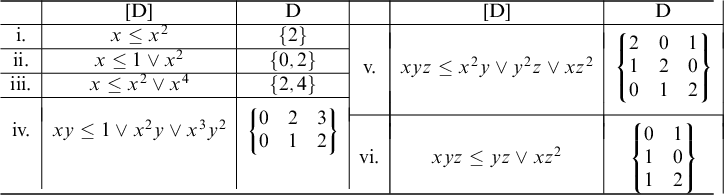
From Table 1, we see that (i) and (ii) are spinal. The simple equation (vi) is prespinal via the $1$ -variable substitution ${\boldsymbol {\sigma }}$ given by ${\boldsymbol {\sigma }}(x)=x$ , ${\boldsymbol {\sigma }}(y)=x$ , and ${\boldsymbol {\sigma }}(z)=1$ , i.e., $\mathsf {CRL} +\mbox {(vi)}\models x^2\leq x$ . On the other hand, no trivial equations are prespinal. The general characterization of whether a simple equation is prespinal will be addressed in Section 8, where it is verified that (iii)–(v) in Table 1 are not prespinal right after Theorem 8.6.

Table 1

Some simple equations viewed as sets of column vectors.

Definition 5.3. A simple equation is called spineless if it is not prespinal. A simple equation $\varepsilon $ for $\mathsf {RL} $ is called spineless if $\varepsilon _{\mathcal {C}}$ is spineless.

To demonstrate the vastness of the collection of spineless equations, we will focus our attention only on $1$ -variable basic equations below. Note that every one-variable basic equation has the form

$$ \begin{align*}x^n\leq \bigvee_{p\in P} x^p ,\end{align*} $$

for some $n>0$ and for some finite subset P of $\mathbb {N}$ such that $P\not = \{0\}$ ; we denote such an equation by $[n,P]$ . Also, note that $[n,P]$ is trivial iff $n \in P$ .

Lemma 5.4. Let $[n,P]$ be a $1$ -variable basic equation. Then the linearization of $[n,P]$ is a spineless simple equation iff $[n,P]$ is trivial or P contains at least two distinct positive integers.

Proof. The simple equation resulting from the linearization over $\mathsf {CRL}$ of $[n,P]$ is

(4) $$ \begin{align} [\mathrm{D}]: \textbf{x}_{n}^{\textbf{1}}\leq \bigvee\left\{\textbf{x}_{n}^d:{d\in \mathbb{N}^n}, \sum_{i=1}^n d(i) \in P \right\}, \end{align} $$

and is equivalent over $\mathsf {CRL}$ to $ [n,P]$ .Footnote ⁶

We prove the contraposition for each direction. For the forward direction, if $P=\{p\}$ , where $0<p \not = n$ , then $[n,P]$ is spinal by definition and hence $[\mathrm {D}]$ is prespinal by its obvious substitution to $[n,P]$ : $x_i\mapsto x$ , for all i.

For the reverse direction, suppose that $[n,P]$ is nontrivial and P contains distinct positive numbers $p>q$ . Then for each $i\leq n$ , the terms $x_i^p$ and $x_i^{q}$ appear as joinands on the right-hand side of $[\mathrm {D}]$ . Let ${\boldsymbol {\sigma }}$ be a monoidal substitution that is non-trivializing for $[\mathrm {D}]$ . Then for some $i\leq n$ , ${\boldsymbol {\sigma }}: x_i\mapsto w$ for some monoid term $w\neq 1$ . So both $w^p$ and $w^{q}$ appear as joinands on the right-hand side of ${\boldsymbol {\sigma }}[\mathrm {D}]$ . Since $p>q>0$ , $w^p\neq 1\neq w^{q}$ , and $\mathsf {CRL}\not \models w^p= w^{q}$ , so ${\boldsymbol {\sigma }}[\mathrm {D}]$ is not spinal, as $w^p$ and $w^q$ contain the same variables. Since ${\boldsymbol {\sigma }}$ was arbitrary, it follows that $[n,P]$ is spineless.⊣

In the following sections we undertake a deep analysis of spineless equations, culminating in Corollary 8.14. To highlight this result, we (re)state it here and we use it right afterwards, in Section 5.3, to obtain results (Theorem 5.9) about the equational theory.

Theorem 5.5. Let $\Gamma $ be a finite set of spineless simple equations, then any variety between $\mathsf {CRL} +\Gamma $ and $\mathsf {RL} $ has an undecidable word problem.

5.3 From quasiequations to equations in $\mathsf {CRL}$

In this section we exploit the fact that in certain varieties certain quasiequations are equivalent to equations to show that even their equational theory is undecidable, making use of Theorem 5.5.

The negative cone of a residuated lattice $\textbf{A}$ is the set $A^-=\{a\in A: a\leq 1\}$ . We will say that a subvariety $\mathcal {V}$ of $\mathsf {CRL} $ is negatively n-potent if the negative cone of each algebra in $\mathcal {V}$ is n-potent, i.e., $\mathcal {V}\models (x\wedge 1)^n= (x\wedge 1)^{n+1}$ (or equivalently, $\mathcal {V}\models (x\wedge 1)^n\leq (x\wedge 1)^{n+1}$ ).

Let t be a term and S be a finite set of terms in the language of $\mathsf {CRL} $ . It can be easily verified thatFootnote ⁷

(5) $$ \begin{align} \begin{array}{r c l} (\exists m\in\mathbb{N})(\exists s_1,\ldots,s_m\in S) ~\mathsf{CRL} &\models&\prod_{i=1}^m (1\wedge s_i)\leq t, \\ \mbox{if and only if}\quad (\exists k\in\mathbb{N})~\mathsf{CRL} &\models& (1\wedge\bigwedge S)^k\leq t. \end{array} \end{align} $$

If $\mathcal {V}\subseteq \mathsf {CRL} $ is a negatively n-potent variety, then we obtainFootnote ⁸

(6) $$ \begin{align} (\exists m\in\mathbb{N})(\exists s_1,\ldots,s_m\in S) ~\mathcal{V}\models\prod_{i=1}^m (1\wedge s_i)\leq t \iff\mathcal{V}\models (1\wedge\bigwedge S)^n\leq t. \end{align} $$

We consider the following quasiequation and equation:

In this way we establish the fact that satisfaction of a quasiequation in a negatively n-potent subvariety of $\mathsf {CRL} $ is equivalent to the satisfaction of a corresponding equation.

Lemma 5.6. If $\mathcal {V}$ is a negatively n-potent subvariety of $\mathsf {CRL} $ and $S\cup \{t\}$ a finite set of terms in the language of $\mathcal {V}$ , then

$$ \begin{align*}\mathcal{V}\models \xi_S(t) \iff \mathcal{V}\models \varepsilon_S^n(t).\end{align*} $$

Proof. Let $\textbf{F}_{\mathcal {V}}$ be the free algebra for $\mathcal {V}$ , and define the congruence $C:=\mathrm {Cg}(\{(1\wedge s, s): s\in S \})$ . We denote the quotient algebra by $\textbf{F}_{\mathcal {V}}/C$ . For a subset X of $\mathrm {F}_{\mathcal {V}}^-$ , we denote by $M(X)$ the convex normal submonoid of $\mathrm {F}_{\mathcal {V}}^-$ generated by X.Footnote ⁹ Observe that

$$ \begin{align*}\begin{array}{ l c l l } & \iff & \text{in } \textbf{F}_{\mathcal{V}}/C, [1\wedge t]_C = [1]_C & \\ & \iff & \mbox{in } \textbf{F}_{\mathcal{V}}, (1\wedge t)\in M(\{ 1\wedge s: s\in S \}) &[6] \\ &\iff &\mbox{in } \textbf{F}_{\mathcal{V}}, (\exists m\in\mathbb{N})(\exists s_1,\ldots,s_m\in S) ~\prod_{i=1}^m (1\wedge s_i)\leq t &[6] \\ &\iff &(\exists m\in\mathbb{N})(\exists s_1,\ldots,s_m\in S) ~ \mathcal{V}\models \prod_{i=1}^m (1\wedge s_i)\leq t &\\ &\iff & \mathcal{V}\models (1\wedge\bigwedge S)^n\leq t &\text{Equation } (6). \end{array}\\[-2.8pc] \end{align*} $$

⊣

For an inequality $p: s\leq t$ , define the term $p^{\to }:= s\to t$ . Let ${\texttt{M}}=(\texttt{R}_k,{\texttt{Q}},{\texttt{P}},q_f)$ be an ACM. Define ${\texttt{P}}^{\to }:=\{p^{\to }: p\in {\texttt{P}}\}.$ Then for ${u}\in A_{{\texttt{M}}}$ , the quasiequation $\mathrm {acc}_{\texttt{M}}({u})$ is equivalent to $\xi _{{\texttt{P}}^{\to }}({u}\to q_f)$ . By Lemma 5.6 and Theorem 4.5, we obtain the following:

Theorem 5.7. Let $\mathcal {V}$ be a subvariety of $\mathsf {CRL} $ containing $\mathbf{W}_{\texttt{M}}^+$ , for some k-ACM ${\texttt{M}}$ and satisfying $(x\wedge 1)^n\leq (x\wedge 1)^{n+1}$ for some $n\geq 1$ . Then deciding membership in the equational theory of $\mathcal {V}$ is at least as hard as deciding membership in ${\mathrm {Acc}}({\texttt{M}})$ .

We say a simple equation $\varepsilon $ is expansive if it has, as a substitution instance, an equation of the form

(7) $$ \begin{align}x^n \leq \bigvee_{j=1}^m x^{n+c_j}, \end{align} $$

for some $n,m\geq 1$ and $c_1,\ldots ,c_m\geq 1$ . It is easy to verify that if $\varepsilon $ is expansive then $\mathsf {CRL}+\varepsilon $ is negatively n-potent. We say a variety is expansive if it satisfies an expansive equation. As a consequence of Lemma 5.4, if a simple equation is the equivalent linearization of an expansive basic equation where $m\geq 2$ then it is spineless. By the theorem above and Theorem 4.5 we obtain the following:

Corollary 5.8. Let $\mathcal {V}$ be an expansive subvariety of $\mathsf {CRL} $ containing $\mathbf{W}_{\texttt{M}}^+$ , for some ACM ${\texttt{M}}$ . Then deciding membership in the equational theory of $\mathcal {V}$ is at least as hard as deciding membership in ${\mathrm {Acc}}({\texttt{M}})$ .

In particular, we prove the following theorem as a consequence of Theorem 5.5 and the corollary above.

Theorem 5.9. If $\Gamma $ is a finite set spineless simple equation containing an expansive equation then variety ${\mathsf {CRL} +\Gamma }$ has an undecidable equational theory.

6 Admissibility

We now begin investigating the required features that a machine should have, in order to achieve the exponential encoding. We begin by formalizing the notion of admissibility and its two natural parts.

Let ${\texttt{M}}=(\texttt{R}_k,{\texttt{Q}},{\texttt{P}}, q_f)$ be a k-ACM and $[\mathrm {D}]$ a n-variable simple equation. We define the relation $\leq ^{\mathrm {D}}$ to be the smallest relation containing

$$ \begin{align*} \textbf{t}_{n}^{\textbf{1}} \leq \bigvee_{d\in\mathrm{D}}\textbf{t}_{n}^d, \end{align*} $$

for all $\textbf{t}_{n}\in (({\texttt{Q}}\cup \texttt{R}_k)^*)^n$ , and closed under the inference rules $[\cdot ]$ and $[\vee ]$ . We define the computation relation $\leq _{\mathrm {D} {\texttt{M}}}$ as the smallest compatible preorder generated by ${\texttt{P}}\cup {\leq }^{\mathrm {D}}$ , and set ${\mathrm {Acc}}(\mathrm {D} {\texttt{M}}):=\{u\in A_{\texttt{M}}: \exists {\texttt{u}}_f\in {\texttt{Fin}}({\texttt{M}}),~u\leq _{\mathrm {D} {\texttt{M}}} {\texttt{u}}_f\}.$

The construction of $\leq _{\mathrm {D}\texttt{M}}$ enjoys an analogue to Lemma 3.1(2), and therefore the following analogue to Lemma 3.4(2):

The frame $\textbf{W}_{\mathrm {D} {\texttt{M}}}$ is defined as $\textbf{W}_{ {\texttt{M}}}$ , but the nuclear relation is defined with respect to ${\mathrm {Acc}}({\mathrm {D}\texttt{M}})$ instead of ${\mathrm {Acc}}({\texttt{M}})$ .

Proof. Let $[\mathrm {D}]$ be an n-variable simple equation where $\mathrm {D}=\{d_1, \ldots , d_m\}$ . It is enough to show that $\textbf{W}_{\mathrm {D} {\texttt{M}}}^+\models [\mathrm {D}]$ . By Theorem 5.1, this is equivalent to showing $\textbf{W}_{\mathrm {D} \texttt{M}}\models (\mathrm {D})$ , i.e., for all $s \in W$ , $\textbf{t}_{n}\in W^n$ ,

If the antecedent of the implication holds, by the definition of $\mathit {N}_{\mathrm {D} {\texttt{M}}}$ and $\leq _{\mathrm {D} {\texttt{M}}}$ and by Lemma 6.1 we obtain

$$ \begin{align*}(\forall d\in \mathrm{D})~\textbf{t}_{n}^{d} ~\mathit{N}_{\mathrm{D} {\texttt{M}}}~ s \iff (\forall d\in \mathrm{D})~ s\textbf{t}_{n}^d\in{\mathrm{Acc}}{(\mathrm{D} {\texttt{M}})} \iff \bigvee_{d\in \mathrm{D}}s\textbf{t}_{n}^d\in{\mathrm{Acc}}{(\mathrm{D} {\texttt{M}})} .\end{align*} $$

Now, by the definition of $\leq _{\mathrm {D} {\texttt{M}}}$ ,

$$ \begin{align*}s \textbf{t}_{n}^{\textbf{1}} \leq_{\mathrm{D} {\texttt{M}}}s\bigvee_{d\in\mathrm{D}}\textbf{t}_{n}^d=\bigvee_{d\in\mathrm{D}} s\textbf{t}_{n}^d ,\end{align*} $$

hence $s \textbf{t}_{n}^{\textbf{1}} \in {\mathrm {Acc}}{(\mathrm {D} {\texttt{M}})} $ and $\textbf{t}_{n}^{\textbf{1}} ~\mathit {N}_{\mathrm {D} {\texttt{M}}}~ s$ . Therefore $\textbf{W}_{\mathrm {D} {\texttt{M}}}^+ \models [\mathrm {D}].$ ⊣

Since ${\leq }_{\texttt{M}} \subseteq {\leq }_{\mathrm {D} {\texttt{M}}}$ , it follows that ${\mathrm {Acc}}({\texttt{M}})\subseteq {\mathrm {Acc}}(\mathrm {D}{\texttt{M}})$ . We say a simple equation $[\mathrm {D}]$ is admissible in a machine ${\texttt{M}}$ if ${\mathrm {Acc}}({\texttt{M}}) = {\mathrm {Acc}}(\mathrm {D} {\texttt{M}})$ . As the only difference between $\textbf{W}_{ {\texttt{M}}}$ and $\textbf{W}_{\mathrm {D} {\texttt{M}}}$ is ${\mathrm {Acc}}({\texttt{M}})$ and ${\mathrm {Acc}}(\mathrm {D} {\texttt{M}})$ , if $[\mathrm {D}]$ is admissible in $\texttt{M}$ then $\textbf{W}^+_{\texttt{M}} = \textbf{W}^+_{\mathrm {D} {\texttt{M}}}$ . Therefore by Lemma 6.2 we obtain the following lemma:

As we will see, admissibility in ${\texttt{M}}$ depends on the machine ${\texttt{M}}$ as well as the equation $[\mathrm {D}]$ . We define the intermediate notions register-admissibility and state-admissibility to make this distinction clear.

For a given ACM ${\texttt{M}}=(\texttt{R}_k,{\texttt{Q}},{\texttt{P}},q_f)$ and n-variable simple equation $[\mathrm {D}]$ , we define $\leq ^{{\mathrm {D}}\texttt{R}}$ to be the smallest relation containing,

$$ \begin{align*} \textbf{x}_{n}^{\textbf{1}} \leq \bigvee_{d\in\mathrm{D}}\textbf{x}_{n}^d,\end{align*} $$

for all $\textbf{x}_{n}\in (\texttt{R}_k^*)^n$ , and closed under the inference rules $[\cdot ]$ and $[\vee ]$ . Define the new computation relation $\leq _{{{\mathrm {D}}\texttt{R}} {\texttt{M}}}$ to be the smallest compatible preorder generated by ${\texttt{P}}\cup {\leq }^{{{\mathrm {D}}\texttt{R}}}$ , and set ${\mathrm {Acc}}({{\mathrm {D}}\texttt{R}} {\texttt{M}}):=\{u\in A_{\texttt{M}}: \exists {\texttt{u}}_f\in {\texttt{Fin}}({\texttt{M}}),~u\leq _{{{\mathrm {D}}\texttt{R}} {\texttt{M}}} {\texttt{u}}_f\}$ . Since the effect of $[\mathrm {D}]$ is restricted to only register terms in $\leq ^{\mathrm {D}\texttt{R}}$ , by the same argument as Lemma 3.4(1), it follows that ${\mathrm {Acc}}({\mathrm {D}}\texttt{R} {\texttt{M}})\subseteq \texttt{ID}(\texttt{M})$ .

It is clear then that ${\mathrm {Acc}}({{\mathrm {D}}\texttt{R}} {\texttt{M}})\subseteq {\mathrm {Acc}}(\mathrm {D} {\texttt{M}})$ , since ${\leq }^{{\mathrm {D}}\texttt{R}}$ is merely a restriction of ${\leq }^{\mathrm {D}}$ . In total, we obtain

$$ \begin{align*} {\mathrm{Acc}}({\texttt{M}})\subseteq{\mathrm{Acc}}({{\mathrm{D}}\texttt{R}} {\texttt{M}})\subseteq {\mathrm{Acc}}(\mathrm{D} {\texttt{M}}).\end{align*} $$

If ${\mathrm {Acc}}({\texttt{M}})={\mathrm {Acc}}({{\mathrm {D}}\texttt{R}} {\texttt{M}})$ , then we say $[\mathrm {D}]$ is register-admissible in ${\texttt{M}}$ . If ${\mathrm {Acc}}({{\mathrm {D}}\texttt{R}} {\texttt{M}})= {\mathrm {Acc}}(\mathrm {D} {\texttt{M}})$ , we say $[\mathrm {D}]$ is state-admissible in ${\texttt{M}}$ . Hence $[\mathrm {D}]$ is admissible in ${\texttt{M}}$ iff $[\mathrm {D}]$ is both register and state-admissible in ${\texttt{M}}$ . Due to the property that instructions in an ACM replace a single state-variable of a configuration by precisely one state-variable, we show in Lemma 6.5 that state-admissibility is a property of the equation $[\mathrm {D}]$ independent of the machine ${\texttt{M}}$ .

6.1 State-admissibility for spineless equations

We say that a simple equation $[\mathrm {D}]$ is mingly if there exists a one-variable substitution ${\boldsymbol {\sigma }}$ such that ${\boldsymbol {\sigma }} [\mathrm {D}] : x^{\lambda } \leq \bigvee _{d \in \mathrm {D}} x$ for some $\lambda>1$ . That is, if $[\mathrm {D}]$ is an equation in n-variables, ${\boldsymbol {\sigma }} (\textbf{x}_{n}^{\textbf{1}})=x^{\lambda }$ and ${\boldsymbol {\sigma }} (\textbf{x}_{n}^{d})=x$ , for all $d \in \mathrm {D}$ .

Of course, this is equivalent over $\mathsf {RL}$ to $x^{\lambda } \leq x$ , but since we do not assume idempotency of $\vee $ in $\textbf{A}_{\texttt{M}}$ , we write $ x^{\lambda } \leq \bigvee _{d \in \mathrm {D}} x$ so as to be explicit about the implementation of the equation in computations.

By definition, mingly equations are prespinal. Equation (vi) from Table 1 is mingly, using the substitution witnessing it is prespinal, while the remaining equations can easily be verified to be not mingly.Footnote ¹⁰ Since mingly equations are prespinal by definition, we obtain the following result.

Lemma 6.4. A spineless equation is non-mingly.

As we will be dealing only with spineless equations, the equations we will consider are not mingly. The following lemma shows that only mingly equations invalidate state-admissibility and also that state-admissibility is independent of the choice of the machine.

Lemma 6.5. The following are equivalent for any ${\texttt{M}}$ and simple equation $[\mathrm {D}]$ .

1. 1. $[\mathrm {D}]$ is state-admissible in ${\texttt{M}}$ .

2. 2. ${\mathrm {Acc}}{(\mathrm {D} {\texttt{M}})}\subseteq \texttt{ID}(\texttt{M})$ .

3. 3. $[\mathrm {D}]$ is not mingly.

Proof. Assume $\texttt{M}=(\texttt{R}_k,\texttt{Q},\texttt{P},q_f)$ and let $[\mathrm {D}]$ be an n-variable simple equation.

( $1\Rightarrow 2$ ) We have that ${\mathrm {Acc}}(\mathrm {D} {\texttt{M}})={\mathrm {Acc}}({\mathrm {D}}\texttt{R} {\texttt{M}})\subseteq \texttt{ID}(\texttt{M})$ .

( $2\Rightarrow 3$ ) Proceeding by contraposition, suppose $[\mathrm {D}]$ is mingly. Then $x^{\lambda } \leq \bigvee _{d \in \mathrm {D}} x$ is a direct substitution image of $[\mathrm {D}]$ , for $\lambda>1$ . For $x=q_f$ , we have

$$ \begin{align*} q_f^{\lambda}\leq^{\mathrm{D}} \bigvee_{d\in\mathrm{D}} q_f \in{\texttt{Fin}}({\texttt{M}})\subseteq{\mathrm{Acc}}(\mathrm{D} {\texttt{M}}). \end{align*} $$

Since $\lambda>1$ , it follows that $q_f^{\lambda }\not \in \texttt{ID}(\texttt{M}).$

( $3\Rightarrow 1$ ) Proceeding by contraposition, suppose ${\mathrm {Acc}}({{\mathrm {D}}\texttt{R}} {\texttt{M}})$ is a proper subset of ${\mathrm {Acc}}(\mathrm {D} {\texttt{M}})$ and let $t\in {\mathrm {Acc}}(\mathrm {D} {\texttt{M}})\setminus {\mathrm {Acc}}({{\mathrm {D}}\texttt{R}} {\texttt{M}})$ be a witness with minimal computation

$$ \begin{align*} t=u_0\leq^{p_1}u_1\leq^{p_2} \cdots\leq^{p_N} u_N ={\texttt{u}}_f\in {\texttt{Fin}}({\texttt{M}}), \end{align*} $$

for some $u_0, u_1,\ldots ,u_N\in A_{\texttt{M}}$ and $p_1,\ldots ,p_N\in {\texttt{P}}\cup \{\mathrm {D}\}$ . Since ${\texttt{Fin}}({\texttt{M}})\subseteq {\mathrm {Acc}}({{\mathrm {D}}\texttt{R}} {\texttt{M}})$ , we have that $t\not \in {\texttt{Fin}}({\texttt{M}})$ and so $N>1$ . By Lemma 6.1, we may assume $t\in ({\texttt{Q}}\cup \texttt{R}_k)^*$ . Since N is minimal, it follows that $p_1 =\mathrm {D} $ and $u_1\in {\mathrm {Acc}}({{\mathrm {D}}\texttt{R}} {\texttt{M}})\subseteq \texttt{ID}(\texttt{M})$ . So,

$$ \begin{align*} t= s\textbf{t}_{n}^{\textbf{1}} \leq^{\mathrm{D}} \bigvee_{d\in\mathrm{D}} s\textbf{t}_{n}^d=u_1, \end{align*} $$

where $s\in ({\texttt{Q}}\cup \texttt{R}_k)^*$ and $\textbf{t}_{n}\in (({\texttt{Q}}\cup \texttt{R}_k)^*)^n$ ; here we used the fact that the rule $[\vee ]$ is not applicable, as $t\in ({\texttt{Q}}\cup \texttt{R}_k)^*$ .

Since $u_1\in \texttt{ID}(\texttt{M})$ , it follows that $s\textbf{t}_{n}^d\in \texttt{Conf}(\texttt{M})$ for all $d\in \mathrm {D}$ . Also, because $p_1\neq \mathrm {D}\texttt{R}$ , there is some $t_i$ that contains at least one state variable. As that $t_i$ must also appear on the right-hand side and $s\textbf{t}_{n}^{\textbf{1}} \in \texttt{Conf}(\texttt{M})$ , it follows that s cannot contain any state variable, so $s \in \texttt{R}_k^*$ . Consequently, every joinand in the right-hand side has a unique $t_i$ containing a state variable.

Therefore, applying the substitution ${\boldsymbol {\sigma }}$ defined by: ${\boldsymbol {\sigma }}(x_i)=x$ if $t_i$ contains a state variable and ${\boldsymbol {\sigma }}(x_i)=1$ otherwise, yields $x^{\lambda } \leq x$ , where $\lambda $ is the number of $t_i$ ’s containing a state variable.

We will show that $\lambda> 1$ . If, by way of contradiction, there was a unique $t_j$ containing a state variable, then it would have the form $t_j=qx$ for some $q\in {\texttt{Q}}$ and $x\in \texttt{R}_k^*$ (with $t_i\in \texttt{R}_k^*$ for all other $t_i$ ’s) and $t_j$ would appear on all the joinands on the right-hand side. So, we have

$$ \begin{align*} t=sqx\prod_{i\not = j} t_i \leq^{\mathrm{{\mathrm{D}}\texttt{R}}}\bigvee_{d\in\mathrm{D}} sqx\prod_{i\not = j}^n{ t_i}^{d(i)}=u_1\in {\mathrm{Acc}}({\mathrm{D}}\texttt{R} {\texttt{M}}), \end{align*} $$

and thus $t\in {\mathrm {Acc}}({\mathrm {D}}\texttt{R} {\texttt{M}}),$ a contradiction.⊣

Therefore, in our search for an appropriate machine for spineless equations, state-admissibility will be automatic and will not restrict the type of possible machines.

7 The exponential encoding

Given a $2$ -ACM ${\texttt{M}}=(\texttt{R}_2,{\texttt{Q}},{\texttt{P}}, q_f)$ (we will later choose as ${\texttt{M}}$ a machine with undecidable halting problem) and simple equation $[\mathrm {D}]$ , our ultimate goal is to construct a new machine ${\texttt{M}}'$ “simulating” the machine ${\texttt{M}}$ such that ${\mathrm {Acc}}(\mathrm {D} {\texttt{M}}' ) = {\mathrm {Acc}}({\texttt{M}}')$ . More specifically, for any spineless equation $[\mathrm {D}]$ we can construct a 3-ACM ${\texttt{M}}_K=(\texttt{R}_3,{\texttt{Q}}_K,{\texttt{P}}_K, q_F)$ for which it will be register-admissible, for some $K>1$ provided by Theorem 8.10, that will simulate the behavior of the 2-ACM ${\texttt{M}}$ in the following way:

$$ \begin{align*}q\texttt{r}_1^{n_1}\texttt{r}_2^{n_2}\in {\mathrm{Acc}}({\texttt{M}}){\text{ if and only if }} q\texttt{r}_1^{K^{n_1}}\texttt{r}_2^{K^{n_2}} \in{\mathrm{Acc}}({\texttt{M}}_K).\end{align*} $$

So, the content n of a register $\texttt{r}$ is not represented by $\texttt{r}^{n}$ but by $\texttt{r}^{K^n}$ . Computationally, this will be achieved by replacing each increment- $\texttt{r}$ (decrement- $\texttt{r}$ ) instruction by a distinct set of instructions (i.e., a program) that will carry out the process of multiplying (dividing) the contents in register $\texttt{r}$ by K. The auxiliary register $\texttt{r}_3$ will be necessary to carry out such computations, and the faithfulness of this encoding will be guaranteed by the insistence that accepted configurations are those which have a computation resulting in a finite join of configurations labeled by state $q_F$ where all the registers are empty.

We will first show how we can achieve multiplying the contents of a register $\texttt{r} \in \texttt{R}_2$ by a fixed constant $K>1$ . Let $\texttt{Q}_{+K}=\{a_0,\ldots ,a_K\}$ be a set of $(K+1)$ -many fresh state-variables. We can add K tokens to the contents of the auxiliary register $\texttt{r}_3$ by starting from the state $a_0$ and applying the instructions $\texttt{P}_{+K}=\{+_i : i=1,\ldots ,K \}$ , where $+_i: a_{i-1}\leq a_i\texttt{r}_3$ , and reaching state $a_K$ . Then for each $0\leq i<K$ , we have

$$ \begin{align*} a_0\leq_{+K} a_i\texttt{r}_3^N \iff N=i , \end{align*} $$

where $\leq _{+K}$ is the computation relation defined in the usual way from $\texttt{P}_{+K}$ . Hence $a_0x\leq _{+K} a_Ky$ iff $y=x\texttt{r}_3^K$ , for each $x,y\in \texttt{R}_3^*$ .

Now, if we have N tokens in register $\texttt{r}$ and we are at state $a_K$ , then by removing one $\texttt{r}$ -token, moving to state $a_0$ by the instruction $\times _{\mathrm {loop}}: a_K\texttt{r}\leq a_0$ , and using $\texttt{P}_{+K}$ to add $K \ \texttt{r}_3$ -tokens and repeating this process, we can essentially exchange $N \ \texttt{r}$ -tokens for $NK \ \texttt{r}_3$ -tokens. For example,

$$ \begin{align*} a_K\texttt{r}^N \leq^{\times_{\mathrm{loop}}} a_0\texttt{r}^{N-1} \leq_{+K}a_K\texttt{r}^{N-1} \texttt{r}_3^{K}\leq^{\times_{\mathrm{loop}}} a_0\texttt{r}^{N-2}\texttt{r}_3^{K}\leq_{+K}\cdots ~a_K\texttt{r}_3^{NK}. \end{align*} $$

If we set $\leq _{\times \texttt{r}}$ to be the computation relation defined from $\texttt{P}_{\texttt{r}\times K}=\texttt{P}_{+K}\cup \{\times _{\mathrm {loop}} \}$ , then it is easily verified by induction that for each $N,M,n,m\in \mathbb {N}$ and $0\leq i \leq K $ :

(8) $$ \begin{align} \begin{array}{r c l} a_K \texttt{r}^N \leq_{\times\texttt{r}} a_i \texttt{r}^n \texttt{r}_3^m &\iff & KN=Kn + m + (K-i),\\ a_i\texttt{r}^n \texttt{r}_3^m\leq_{\times\texttt{r}} a_K\texttt{r}_3^M &\iff& M=Kn+m + (K-i). \end{array} \end{align} $$

Observe that multiplying the contents of register $\texttt{r}$ is achieved by an iterative process of adding K-many tokens to $\texttt{r}_3$ and then looping the process by removing one from $\texttt{r}$ . We can define a division program analogously. However, in both cases, we start with tokens in $\texttt{r}$ and compute the product (or quotient) by K in the register $\texttt{r}_3$ by emptying $\texttt{r}$ . We would then like our machine to transfer those contents back to the original register $\texttt{r}$ to complete this program.

Let $\texttt{T}_{\texttt{r}}$ be the program with fresh states $\texttt{Q}_{\texttt{T}_{\texttt{r}}}=\{t_0,t_1 \}$ and instructions $\texttt{P}_{\texttt{T}_{\texttt{r}}}=\{T_-,T_+ \}$ given by $T_-: t_0\texttt{r}_3\leq t_1$ and $T_+: t_1\leq t_0\texttt{r}$ . Defining its computation relation to be $\leq _{\texttt{T}_{\texttt{r}}}$ , we easily obtain for all $N,M,n,m\in \mathbb {N}$ :

(9) $$ \begin{align} \begin{array}{r c l} t_0 \texttt{r}_3^N \leq_{\texttt{T}_{\texttt{r}}} t_{\delta} \texttt{r}^n\texttt{r}_3^m &\iff &N=n+m+\delta, \\ t_{\delta} \texttt{r}^n\texttt{r}_3^m\leq_{\texttt{T}_{\texttt{r}}} t_0\texttt{r}^M&\iff& n+m+\delta=M. \end{array} \end{align} $$

If we wish to implement the transfer program after, say, executing the program for multiplying by K, then we need an instruction to switch from the state $a_0$ to the state $t_0$ . This can naively be achieved by a forking instruction, say $p:a_K\leq t_0$ ,Footnote ¹¹ which would allow for the computation

$$ \begin{align*} a_K\texttt{r}^N \leq_{\times \texttt{r}}a_K\texttt{r}_3^{NK} \leq^p t_0\texttt{r}_3^{NK} \leq_{\texttt{T}_{\texttt{r}}}t_0\texttt{r}^{NK}.\end{align*} $$

However, since the instruction p can be applied to any configuration labeled by $a_K$ , even those for which the register $\texttt{r}$ is nonempty, we also get unwanted instances of the form $a_K\texttt{r}^N\leq t_0\texttt{r}^{M}$ where $M=Km+N-m$ for each $0\leq m\leq N$ . Since we want our simulation to be faithful, we need a way of switching to the transfer program only when the register $\texttt{r}$ is empty.

7.1 The zero-test program

What we are asking for is similar to (what is commonly called) a zero-test instruction of a standard counter machine, i.e., an instruction which is applicable only when a specified register is empty. Since we require our computation relations to be compatible with multiplication, such an insistence is impossible. That is, we insist $q\leq q'$ to entail $qx\leq q'x$ for any term x.

However, following the ideas in [Reference Lothaire11], we construct a program that has a similar behavior utilizing the insistence that accepted configurations are those that compute final ID’s, i.e., finite joins of the configuration labeled by a final state $q_F$ with all registers empty.

We define the (sub-)machine ${\unicode{xf8} }=(\texttt{R}_3,{\texttt{Q}}_{\unicode{xf8} }, {\texttt{P}}_{\unicode{xf8} },q_F)$ , with a fresh set of variables ${\texttt{Q}}_{\unicode{xf8} } = \{z_1,z_2,z_3,q_F\}$ and instructions ${\texttt{P}}_{\unicode{xf8} }$ are given by:

$$ \begin{align*}\begin{array}{ l c r c l } {{\unicode{xf8}}^i_j}&:&z_i \texttt{r}_j&\leq& z_i, \\ {{\unicode{xf8}}^i_F}&:& z_i&\leq& q_F\vee q_F, \end{array}\end{align*} $$

for each $i, j\in \{1,2,3\}$ with $i \not = j$ , resulting in a total of $6+3=9$ instructions.

The addition of the auxiliary states $z_1, z_2, z_3$ is explained by the fact that the role of $z_i$ is to empty the contents of all registers other than $\texttt{r}_i$ and transition to the final state $q_F$ . Thus it detects situations where $\texttt{r}_i$ is not already empty, as then it cannot reach a final ID. So, assuming we want to move from state $q_{\mathrm {in}}$ to $q_{\mathrm {out}}$ only when the register $\texttt{r}_i$ is empty, we can start a parallel computation, the main branch of which moves to state $q_{\mathrm {out}}$ (even if $\texttt{r}_i$ is non-empty) but the auxiliary branch involving the $z_i$ terminates successfully only if $\texttt{r}_i$ is empty. This $z_i$ -branch ensures/safeguards that the combined computation acts as intended.

We call the above machine the zero-test program, and we denote its computation relation by $\leq _{\unicode{xf8} }$ . The zero-test program for a register $\texttt{r}_i$ is implemented by a zero-test $\texttt{r}_i$ instruction p, where p is of the form $q_{\mathrm {in}} \leq q_{\mathrm {out}}\vee z_i$ . Since the desired final ID’s of ${\texttt{M}}_K$ will consist of only joins of the configuration $q_F$ , i.e., all registers are empty, the above instruction copies the contents of the registers and creates two paths; one path with the state $q_{\mathrm {out}}$ where $\texttt{r}_i$ is intended to be empty, and the second with a state $z_i$ where the program ${\unicode{xf8} }$ is intended to empty registers $\texttt{r}_j$ and $\texttt{r}_k$ and then output to the final state. Below is an example of implementing the zero-test on register $\texttt{r}_1$ via the instruction $p:q_{\mathrm {in}}\leq q_{\mathrm {out}}\vee z_1$ on the configuration $q_{\mathrm {in}} \texttt{r}_1\texttt{r}_2\texttt{r}_3$ :

$$ \begin{align*}\begin{array} {r l l} q_{\mathrm{in}} \texttt{r}_1\texttt{r}_2\texttt{r}_3 &\leq^{p}&q_{\mathrm{out}} \texttt{r}_1\texttt{r}_2\texttt{r}_3\vee z_1\texttt{r}_1\texttt{r}_2\texttt{r}_3 \\ &\leq^{{\unicode{xf8}}^1_2}&q_{\mathrm{out}} \texttt{r}_1\texttt{r}_2\texttt{r}_3\vee z_1\texttt{r}_1\texttt{r}_3 \\ &\leq^{{\unicode{xf8}}^1_3}&q_{\mathrm{out}} \texttt{r}_1\texttt{r}_2\texttt{r}_3\vee z_1\texttt{r}_1 \\ &\leq^{{\unicode{xf8}}^1_F}&q_{\mathrm{out}} \texttt{r}_1\texttt{r}_2\texttt{r}_3\vee q_F\texttt{r}_1 \vee q_F\texttt{r}_1. \end{array}\end{align*} $$

As we see, the above (maximal in $\unicode{xf8} )$ computation detected that register $\texttt{r}_1$ is not empty in the configuration $q\texttt{r}_1\texttt{r}_2\texttt{r}_3$ since the final ID contains the configuration $q_F\texttt{r}_1$ , and there are no $q_F$ -instructions. In fact, $z_1\texttt{r}_1\texttt{r}_2\texttt{r}_3\not \in {\mathrm {Acc}}(\unicode{xf8} )$ since there is no instruction applicable to the state $z_1$ which alters the contents of register $\texttt{r}_1$ . By a similar analysis, we obtain the following:

Lemma 7.1. $z_i\texttt{r}_1^{n_1}\texttt{r}_2^{n_2}\texttt{r}_3^{n_3}\in {\mathrm {Acc}}(\unicode{xf8} )$ if and only if $n_i=0$ .

Let $\mathcal {P}$ be a program (i.e., a sub-machine) and $\leq _{\mathcal {P}}$ be its corresponding computation relation. We define the relation $\sqsubseteq _{\mathcal {P}}$ on $\texttt{Conf}({\mathcal {P}})$ via ${\texttt{C}}\sqsubseteq _{\mathcal {P}} {\texttt{C}'}$ iff ${\texttt{C}}\leq _{\mathcal {P}} {\texttt{C}'}\vee u$ , where either $u=\bot $ or $u\in \mathrm {ID}({\unicode{xf8} }) $ with $u\in {\mathrm {Acc}}(\unicode{xf8} )$ .Footnote ¹² If $\mathcal {P}$ contains no ${\texttt{Q}}_{\unicode{xf8} }$ -instructions (i.e., no instruction $z_ix\leq \cdots $ ), then ${\texttt{C}}\sqsubseteq _{\mathcal {P}}{\texttt{C}'}$ iff there is a computation from ${\texttt{C}}$ to ${\texttt{C}'}\vee u$ with instructions from $\mathcal {P}$ such that every zero-test was properly applied. Note that $\sqsubseteq _{\mathcal {P}}$ is transitive on configurations and ${\texttt{C}}\leq _{\mathcal {P}} {\texttt{C}'}$ implies ${\texttt{C}}\sqsubseteq _{\mathcal {P}} {\texttt{C}'}$ . We obtain the following lemma.

Lemma 7.2. Let p be the instruction $q_{\mathrm {in}}\leq q_{\mathrm {out}}\vee z_i$ with distinct $q_{\mathrm {in}}, q_{\mathrm {out}}\not \in {\texttt{Q}}_{\unicode{xf8} }$ . For $x,x'\in \texttt{R}_3^*$ , $q_{\mathrm {in}} x \sqsubseteq _{\{p\}} q_{\mathrm {out}} x'$ if and only if $x=x'=\texttt{r}_1^{n_1}\texttt{r}_2^{n_2}\texttt{r}_3^{n_3}$ and $n_i=0$ .

Proof. Let $x=\texttt{r}_1^{n_1}\texttt{r}_2^{n_2}\texttt{r}_3^{n_3}$ . The only instruction applicable to $q_{\mathrm {in}} x$ is p, so from $q_{\mathrm {in}}\leq q_{\mathrm {out}}\vee z_i$ we obtain $q_{\mathrm {in}} x\leq ^p q_{\mathrm {out}} x\vee z_i x$ . Since the only instructions applicable are those from $\{p\}$ and $q_{\mathrm {in}}\neq q_{\mathrm {out}}$ , the computation cannot proceed from this configuration. Hence by Lemma 7.1,

$$ \begin{align*}q_{\mathrm{in}} x \sqsubseteq_{\{p\}} q_{\mathrm{out}} x' \iff x=x' \text{ and } z_ix\leq_{{\unicode{xf8}}} q_F\iff x=x' \text{ and } n_i=0.\\[-2.8pc] \end{align*} $$

⊣

7.2 Multiplying and dividing

We are now ready to faithfully simulate an increment- $\texttt{r}$ instruction by a program that multiplies the contents of register $\texttt{r} \in \{\texttt{r}_1, \texttt{r}_2\}$ by the fixed constant K. For $p: q_{\mathrm {in}}\leq q_{\mathrm {out}} \texttt{r}$ , we define the program ${\times }(p)$ to have states $\texttt{Q}_{\times (p)}=\texttt{Q}_{+K}\cup \texttt{Q}_{\texttt{T}_{\texttt{r}}}$ and instructions $\texttt{P}_{\times (p)}=\texttt{P}_{+K}\cup \texttt{P}_{\texttt{T}_{\texttt{r}}}\cup \{\times _{\mathrm {in}}, \times _{\texttt{T}},\times _{\mathrm {out}} \}$ , where

$$ \begin{align*}\begin{array}{l c r c l } {\times_{\mathrm{in}}}&:& q_{\mathrm{in}} &\leq& a_K\vee z_3, \\ {\times_{\texttt{T}}} &:& a_K &\leq& t_0\vee z_i, \\ {\times_{\mathrm{out}}} &:& t_0&\leq& q_{\mathrm{out}} \vee z_3. \end{array}\end{align*} $$

The instruction $\times _{\mathrm {in}}$ is intended to verify that the auxiliary register $\texttt{r}_3$ is in fact empty, and initiate the process of storing in $\texttt{r}_3 \ K$ -times the contents in the active register $\texttt{r}$ . The instruction $\times _{\texttt{T}}$ is meant to check that all the contents of the active register $\texttt{r}$ have been emptied (and thus K-times that amount is in $\texttt{r}_3$ ), and initiate the transfer program. The instruction $\times _{\mathrm {out}}$ is intended to end the program by transitioning to the state $q_{\mathrm {out}}$ only when the transfer is complete, i.e., when $\texttt{r}_3$ has been emptied. Below is an example of $\times (q_{\mathrm {in}}\leq q_{\mathrm {out}} \texttt{r}_1)$ running on the configuration $q_{\mathrm {in}} \texttt{r}_1^2\texttt{r}_2$ :

$$ \begin{align*}\begin{array}{r l l} q_{\mathrm{in}} \texttt{r}_1^2\texttt{r}_2 & \sqsubseteq_{\{\times_{\mathrm{in}}\}}& a_K\texttt{r}_1^2 \texttt{r}_2\\ &\leq_{\times_{\texttt{r}_1}}& a_K\texttt{r}_2\texttt{r}_3^{2K}\\ &\sqsubseteq_{\{\times_{\texttt{T}}\}} &t_0\texttt{r}_2\texttt{r}_3^{2K}\\ &\leq_{\texttt{T}_{\texttt{r}_1}}&t_0 \texttt{r}_1^{2K}\texttt{r}_2\\ &\sqsubseteq_{\{ \times_{\mathrm{out}}\}}&q_{\mathrm{out}} \texttt{r}_1^{2K}\texttt{r}_2. \end{array}\end{align*} $$

In this way, we obtain the following technical lemma by induction as a consequence of Lemma 7.2 and Equations (8) and (9). We state the lemma for $\texttt{r}=\texttt{r}_1$ , but the same holds when swapping the roles of $\texttt{r}_1$ and $\texttt{r}_2$ .

Lemma 7.3. Let $p: q_{\mathrm {in}}\leq q_{\mathrm {out}}\texttt{r}_1$ be an increment- $\texttt{r}_1$ instruction, where $q_{\mathrm {in}}, q_{\mathrm {out}} \not \in \texttt{Q}_{\times (p)}$ . Then

$$ \begin{align*} q_{\mathrm{in}} \texttt{r}_1^{N_1}\texttt{r}_2^{N_2}\texttt{r}_3^{N_3} \sqsubseteq_{\times(p)} q_{\mathrm{out}} \texttt{r}_1^{M_1}\texttt{r}_2^{M_2}\texttt{r}_3^{M_3}, \end{align*} $$

if and only if $M_1=KN_1$ , $M_2=N_2$ , and $M_3=N_3=0$ . In fact, for each $n_1,n_2,n_3\in \mathbb {N}$ and state $q\in \texttt{Q}_{\times (p)} $ ,

1. 1. $q_{\mathrm {in}} \texttt{r}_1^{N_1}\texttt{r}_2^{N_2}\texttt{r}_3^{N_3} \sqsubseteq _{\times (p)} q\texttt{r}_1^{n_1}\texttt{r}_2^{n_2}\texttt{r}_3^{n_3}$ iff $N_3=0$ , $N_2=n_2$ , and

   $$ \begin{align*}KN_1 = \left\{\begin{array}{r l} n_1+n_3+\delta & \mbox{if } q=t_{\delta} \mbox{ where } \delta\in \{0,1\},\\ Kn_1+n_3+(K-\delta) & \mbox{if }q=a_{\delta} \mbox{ where } 0\leq \delta\leq K. \end{array}\right.\end{align*} $$

2. 2. $q\texttt{r}_1^{n_1}\texttt{r}_2^{n_2}\texttt{r}_3^{n_3} \sqsubseteq _{\times (p)} q_{\mathrm {out}} \texttt{r}_1^{M_1}\texttt{r}_2^{M_2}\texttt{r}_3^{M_3} $ iff $M_3=0$ , $M_2=n_2$ , and

   $$ \begin{align*}M_1 = \left\{\begin{array}{r l} n_1+n_3+\delta & \mbox{if } q=t_{\delta} \mbox{ where } \delta\in \{0,1\},\\ Kn_1+n_3+(K-\delta) & \mbox{if }q=a_{\delta} \mbox{ where } 0\leq \delta\leq K. \end{array}\right.\end{align*} $$

For a configuration $\texttt{C}=q\texttt{r}_1^n\texttt{r}_2^m$ in $\texttt{M}$ , by $\texttt{C}_K$ we denote the configuration $q\texttt{r}_1^{K^n}\texttt{r}_2^{K^m}$ in $\texttt{M}_K$ .

Corollary 7.4. Let p be an increment instruction from some $2$ -ACM $\texttt{M}$ . Then $\texttt{C}\leq ^p\texttt{C}'$ if and only if $\texttt{C}_K\sqsubseteq _{\times (p)}\texttt{C}^{\prime }_K$ for any configurations $\texttt{C},\texttt{C}'$ in $\texttt{Conf}(\texttt{M})$ .

In a completely analogous way, given a decrement- $\texttt{r}$ instruction $p:q_{\mathrm {in}}\texttt{r}\leq q_{\mathrm {out}} $ , we define the division by K program $\div (p)$ as follows. For its set of states $\texttt{Q}_{\div (p)}$ , we define a fresh set of states $\texttt{Q}_{\texttt{r}-K}=\{s_0,\ldots ,s_K \}$ and set $\texttt{Q}_{\div (p)}=\texttt{Q}_{\texttt{r}-K}\cup \texttt{Q}_{\texttt{T}_{\texttt{r}}}$ . We take as its instructions $\texttt{P}_{\div (p)}= \texttt{P}_{\texttt{r}-K}\cup \texttt{P}_{\texttt{T}_{\texttt{r}}}\cup \{\div _{\mathrm {in}},\div _{\texttt{T}},\div _{\mathrm {out}} \}$ , where $\texttt{P}_{\texttt{r}-K}$ contains the instruction $\div _{\mathrm {loop}}: s_K\leq s_0\texttt{r}_3$ and K-many instructions of the form $-_i:s_{i-1}\texttt{r}\leq s_i $ , for $1\leq i\leq K$ , and finally

$$ \begin{align*}\begin{array}{l c r c l} {\div_{\mathrm{in}}}&:& q_{\mathrm{in}} &\leq& s_0\vee z_3, \\ {\div_{\texttt{T}}} &:& s_0 &\leq& t_0\vee z_i, \\ {\div_{\mathrm{out}}} &:& t_0&\leq& q_{\mathrm{out}} \vee z_3. \end{array}\end{align*} $$

The instruction $\div _{\mathrm {in}}$ is intended to verify that the auxiliary register $\texttt{r}_3$ is in fact empty, and initiate the process of storing in $\texttt{r}_3$ the quotient by K of the contents in the active register $\texttt{r}$ . The instruction $\times _{\texttt{T}}$ is meant to check that all the contents of the active register $\texttt{r}$ have been emptied (and thus K-divided by that amount is in $\texttt{r}_3$ ), and initiate the transfer program. The instruction $\div _{\mathrm {out}}$ is intended to end the program transitioning to the state $q_{\mathrm {out}}$ only when the transfer is complete, i.e., when $\texttt{r}_3$ has been emptied. Below is an example of $\div (q_{\mathrm {in}}\texttt{r}_1\leq q_{\mathrm {out}})$ running on the configuration $q_{\mathrm {in}} \texttt{r}_1^{2K}\texttt{r}_2$ :

$$ \begin{align*}\begin{array}{r l l} q_{\mathrm{in}} \texttt{r}_1^{2K}\texttt{r}_2 & \sqsubseteq_{\{\div_{\mathrm{in}}\}}& s_0\texttt{r}_1^{2K} \texttt{r}_2\\ &\leq_{\texttt{r}_1-K}& s_K\texttt{r}_1^K\texttt{r}_2\\ &\leq^{\div_{\mathrm{loop}}}& s_0\texttt{r}_1^K\texttt{r}_2\texttt{r}_3\\ &\leq_{\texttt{r}_1-K}& s_K\texttt{r}_2\texttt{r}_3\\ &\leq^{\div_{\mathrm{loop}}}& s_0\texttt{r}_2\texttt{r}_3^2\\ &\sqsubseteq_{\{\div_{\texttt{T}}\}} &t_0\texttt{r}_2\texttt{r}_3^{2}\\ &\leq_{\texttt{T}_{\texttt{r}_1}}&t_0 \texttt{r}_1^{2}\texttt{r}_2\\ &\sqsubseteq_{\{ \div_{\mathrm{out}}\}}&q_{\mathrm{out}} \texttt{r}_1^{2}\texttt{r}_2. \end{array}\end{align*} $$

The following technical lemma is easily verified by induction. We state the lemma for $\texttt{r}=\texttt{r}_1$ , but the same holds by swapping the roles of $\texttt{r}_1$ and $\texttt{r}_2$ .

Lemma 7.5. Let $p: q_{\mathrm {in}}\texttt{r}_1\leq q_{\mathrm {out}}$ be a decrement- $\texttt{r}_1$ instruction. Then

$$ \begin{align*} q_{\mathrm{in}} \texttt{r}_1^{N_1}\texttt{r}_2^{N_2}\texttt{r}_3^{N_3} \sqsubseteq_{\div(p)} q_{\mathrm{out}} \texttt{r}_1^{M_1}\texttt{r}_2^{M_2}\texttt{r}_3^{M_3}, \end{align*} $$

if and only if $KM_1=N_1>0$ , $M_2=N_2$ , and $M_3=N_3=0$ . In fact, for each $n_1,n_2,n_3\in \mathbb {N}$ and state $q\in \texttt{Q}_{\div (p)} $ ,

1. 1. $q_{\mathrm {in}} \texttt{r}_1^{N_1}\texttt{r}_2^{N_2}\texttt{r}_3^{N_3} \sqsubseteq _{\div (p)} q\texttt{r}_1^{n_1}\texttt{r}_2^{n_2}\texttt{r}_3^{n_3}$ iff $N_3=0$ , $N_2=n_2$ , and

   $$ \begin{align*}N_1 = \left\{\begin{array}{r l} n_1+n_3+\delta & \mbox{if } q=t_{\delta} \mbox{ where } \delta\in \{0,1\}, \\ Kn_1+n_3+(K-\delta) & \mbox{if }q=s_{\delta} \mbox{ where } 0\leq \delta\leq K. \end{array}\right.\end{align*} $$

2. 2. $q\texttt{r}_1^{n_1}\texttt{r}_2^{n_2}\texttt{r}_3^{n_3} \sqsubseteq _{\times (p)} q_{\mathrm {out}} \texttt{r}_1^{M_1}\texttt{r}_2^{M_2}\texttt{r}_3^{M_3} $ iff $M_3=0$ , $M_2=n_2$ , and

   $$ \begin{align*}KM_1 = \left\{\begin{array}{r l} n_1+n_3+\delta & \mbox{if } q=t_{\delta} \mbox{ where } \delta\in \{0,1\},\\ Kn_1+n_3+(K-\delta) & \mbox{if }q=s_{\delta} \mbox{ where } 0\leq \delta\leq K. \end{array}\right.\end{align*} $$

Corollary 7.6. Let p be a decrement instruction from some $2$ -ACM $\texttt{M}$ and $\texttt{C},\texttt{C}'$ be configurations in $\texttt{M}$ . Then $\texttt{C}\leq ^p\texttt{C}'$ if and only if $\texttt{C}_K\sqsubseteq _{\div (p)}\texttt{C}^{\prime }_K$ .

Corollary 7.7. Assume that $p:q_{\mathrm {in}}\texttt{r}\leq q_{\mathrm {out}}$ is a decrement instruction, $\texttt{C}_{\mathrm {in}}$ is a $q_{\mathrm {in}}$ -configuration, $\texttt{C}$ is a $\texttt{Q}_{\div (p)}$ -configuration, and $\texttt{C}_{\mathrm {out}}$ is $q_{\mathrm {out}}$ -configuration. If $\texttt{C}_{\mathrm {in}}\sqsubseteq _{\div (p)}\texttt{C}$ and $\texttt{C}_{\mathrm {in}}\sqsubseteq _{\div (p)} \texttt{C}_{\mathrm {out}}$ , then $\texttt{C}\sqsubseteq _{\div (p)}\texttt{C}_{\mathrm {out}}$ .

Proof. Since $\texttt{C}_{\mathrm {in}}\sqsubseteq _{\div (p)}\texttt{C}$ and $\texttt{C}_{\mathrm {in}}\sqsubseteq _{\div (p)} \texttt{C}_{\mathrm {out}}$ , by Lemma 7.5 the values of $\texttt{C}_{\mathrm {in}}$ and $\texttt{C}$ , as well as the values of $\texttt{C}_{\mathrm {in}}$ and $\texttt{C}_{\mathrm {out}}$ are linked. Therefore, the values of $\texttt{C}_{\mathrm {out}}$ and $\texttt{C}$ are also linked and hence by Lemma 7.5 we obtain $\texttt{C}\sqsubseteq _{\div (p)}\texttt{C}_{\mathrm {out}}$ .⊣

7.3 Construction of ${\texttt{M}}_K$

Let $\texttt{M}=(\texttt{R}_2,\texttt{Q},\texttt{P},q_f)$ be a $2$ -ACM and let $K>1$ be an integer. Since the configuration $q_f$ is accepted in $\texttt{M}$ by definition, we will need $(q_f)_K=q_f\texttt{r}_1\texttt{r}_2$ to be accepted in $\texttt{M}_K$ . To accommodate this, we define the end program as follows. For a fresh variable $c_F$ , we define the set of states ${\texttt{Q}}_F=\{c_F\}$ and the set of instructions ${\texttt{P}}_F=\{F_1,F_2\}$ by:

$$ \begin{align*}\begin{array}{l c r c l } F_1&:& q_f\texttt{r}_1&\leq& c_F, \\ F_2&:& c_F\texttt{r}_2&\leq& q_F. \end{array} \end{align*} $$

By $\leq _F$ we denote the computation relation for the end program.

Lemma 7.8. For $q\in \texttt{Q}_{F}\cup \{q_f\}$ , $q\texttt{r}_1^{n_1}\texttt{r}_2^{n_2}\texttt{r}_3^{n_3}\leq _F q_F$ if and only if $n_3=0$ and

$$ \begin{align*} (n_1,n_2)=\left\{\begin{array}{rl} (1,1)&\text{if } q=q_f, \\ (0,1) &\text{if } q=c_F, \\ (0,0) &\text{if } q=q_F. \end{array}\right.\end{align*} $$

We write the instructions $\texttt{P}$ of $\texttt{M}$ as the disjoint union $\texttt{P}_+\cup \texttt{P}_-\cup \texttt{P}_{\vee }$ of its increment, decrement, and forking instructions, respectively. We can now formally define the $3$ -ACM simulation of $\texttt{M}$ to be the machine ${\texttt{M}}_K=(\texttt{R}_3,\texttt{Q}_K,\texttt{P}_K,q_F)$ , where

• • $\texttt{Q}_K$ is the (disjoint) union of $\texttt{Q}$ , $\texttt{Q}_{\unicode{xf8} }$ , $\texttt{Q}_{F}$ , $\texttt{Q}_{\times (p)}$ for each ${p\in \texttt{P}_+}$ , and $\texttt{Q}_{\div (p)}$ for each $p\in \texttt{P}_-$ .

• • $\texttt{P}_K$ is the (disjoint) union of $\texttt{P}_{\vee }$ , $\texttt{P}_{\unicode{xf8} }$ , $\texttt{P}_{F}$ , $\texttt{P}_{\times (p)}$ for each ${p\in \texttt{P}_+}$ , and $\texttt{P}_{\div (p)}$ for each ${p\in \texttt{P}_-}$ .

• • $q_F$ is the final state of $\texttt{M}_K$ .

Formally, we view all states and instructions in some multiply/divide program $\mathcal {P}(p)$ (where p is an increment/decrement instruction from $\texttt{M}$ ) as being labeled by the instruction p, e.g., a state from $\texttt{Q}_{\mathcal {P}(p)}$ is of the form $q^p$ , and an instruction $\texttt{P}_{\mathcal {P}(p)}$ is of the form $\rho ^p$ . In other words, we make states and instructions in each subprogram disjoint. In fact, since there are no instructions in $\mathcal {P}(p)$ of the form $\cdots \leq q_F\cdots $ , we obtain the following useful observation.

Lemma 7.9. Let p be an increment or decrement instruction from $\texttt{M}$ and $\mathcal {P}(p)$ its corresponding program in $\texttt{M}_K$ . If $\texttt{C}$ is a configuration in $\texttt{M}_K$ labeled by a state from $\texttt{Q}_{\mathcal {P}(p)}$ then the only instructions applicable to $\texttt{C}$ are those from $\texttt{P}_{\mathcal {P}(p)}$ . Furthermore, if $q_{\mathrm {out}}$ is the output state of p, then $\texttt{C}$ being accepted in $\texttt{M}_K$ implies $\texttt{C}\sqsubseteq _{\mathcal {P}(p)} \texttt{C}'\in \mathrm {Acc}(\texttt{M}_K)$ , where $\texttt{C}'$ is labeled by $q_{\mathrm {out}}$ .

Recall, for a configuration $\texttt{C}=q\texttt{r}_1^n\texttt{r}_2^m$ in $\texttt{M}$ , by $\texttt{C}_K$ that we denote the configuration $q\texttt{r}_1^{K^n}\texttt{r}_2^{K^m}$ in $\texttt{M}_K$ .

Lemma 7.10. The following hold for any 2-ACM $\texttt{M}=(\texttt{R}_2,\texttt{Q},\texttt{P},q_f)$ and $K>1$ .

1. 1. A configuration $\texttt{C}$ is accepted in $\texttt{M}$ iff $\texttt{C}_K$ is accepted in $\texttt{M}_K$ . Furthermore, any accepted configuration in $\texttt{M}_K$ labeled by a state from $\texttt{Q}$ must be of the form $\texttt{C}_K$ where $\texttt{C}$ is accepted in $\texttt{M}$ .

2. 2. Let p be an increment or decrement instruction of $\texttt{M}$ and $\texttt{C}$ a configuration of the corresponding program $\mathcal {P}(p) \ (\mathcal {P}\in \{\times ,\div \})$ . Then $\texttt{C}$ is accepted in $\texttt{M}_K$ iff there are accepted configurations $\texttt{C}',\texttt{C}"$ in $\texttt{M}$ such that $\texttt{C}'\leq ^p\texttt{C}"$ and $\texttt{C}^{\prime }_K\sqsubseteq _{\mathcal {P}(p)} \texttt{C}\sqsubseteq _{\mathcal {P}(p)} \texttt{C}^{\prime \prime }_K$ .

Proof. For (1), let $\texttt{C}$ be a configuration in $\texttt{M}$ . Since there are no $q_f$ -instructions in $\texttt{M}$ by definition, if $\texttt{C}$ is labeled by state $q_f$ then it is accepted in $\texttt{M}$ iff $\texttt{C}=q_f$ , i.e., both registers $\texttt{r}_1$ and $\texttt{r}_2$ are empty. By definition, the only $q_f$ -instructions in $\texttt{M}_K$ are those found in the end program. By Lemma 7.8, the only accepted configuration in $\texttt{M}_K$ labeled by $q_f$ is $\texttt{C}_K$ . Now, suppose p is a q-instruction from $\texttt{M}$ . Clearly, if p is a forking instruction, then $\texttt{C}\leq ^p \texttt{C}'\vee \texttt{C}"$ in $\texttt{M}$ iff $\texttt{C}_K\leq ^p \texttt{C}^{\prime }_K\vee \texttt{C}_K"$ . Otherwise, p is an increment or decrement instruction, and by Corollaries 7.4 and 7.6, $\texttt{C}\leq ^p \texttt{C}'$ in $\texttt{M}$ iff $\texttt{C}_K\sqsubseteq _{\mathcal {P}(p)} \texttt{C}_K'$ in $\texttt{M}_K$ . The claim therefore follows by induction on the computation lengths.

For (2), consider a configuration $\texttt{C}$ in $\texttt{M}_K$ labeled by a state from some program $\mathcal {P}(p)$ , where p is an increment or decrement instruction from $\texttt{M}$ . Let $q_{\mathrm {in}}$ and $q_{\mathrm {out}}$ be the input and output states of p, respectively. By Lemma 7.9, we conclude that if a computation witnesses $\texttt{C}$ being accepted in $\texttt{M}_K$ it must implement the output instruction of $\mathcal {P}(p)$ . That is $\texttt{C}\sqsubseteq _{\mathcal {P}(p)}q_{\mathrm {out}} \texttt{r}_1^{n_1}\texttt{r}_2^{n_2}\texttt{r}_3^{n_3}$ . By (1), $n_1$ and $n_2$ are powers of K while $n_3=0$ . By Lemmas 7.3 and 7.5, the result follows.⊣

Let $\tilde {\texttt{M}}$ be the 2-ACM given by Theorem 3.2. Since membership of ${\mathrm {Acc}}(\tilde {\texttt{M}})$ is undecidable, we obtain the following consequence of Lemma 7.10(1):

Corollary 7.11. Membership in the set ${\mathrm {Acc}}(\tilde {\texttt{M}}_K)$ is undecidable for $K>1$ .