Introduction
Accurate and detailed bathymetry maps or digital elevation models (DEMs) are fundamental spatial datasets for conducting marine science research in Antarctica. High-resolution DEMs are not only useful for updating traditional nautical charts for navigational safety, but the new information gained by understanding the sea floor geomorphic relief underpins major oceanographic, biological, geological and glaciological research in offshore Antarctica. Modern surveys using research vessels equipped with multibeam swath echosounders now provide detailed physiographic relief that reveal significant new insights on the physical processes influencing the Antarctic sea floor. Examples of the palaeoglacial and sedimentological processes interpreted through recent multibeam surveys include sites in the Amundsen Sea (Larter et al. Reference Larter, Graham, Gohl, Kuhn, Hillenbrand, Smith, Deen, Livermore and Schenke2009, Smith et al. Reference Smith, Hillenbrand, Larter, Graham and Kuhn2009), Bellingshausen Sea (Heroy & Anderson Reference Heroy and Anderson2005, Dowdeswell et al. Reference Dowdeswell, O’Cofaigh, Noormets, Larter, Hillenbrand, Benetti, Evans and Pudsey2008b, Noormets et al. Reference Noormets, Dowdeswell, Larter, O’Cofaigh and Evans2009), Bransfield basin (Barclay et al. Reference Barclay, Wilcock and Ibanez2009), Antarctic Peninsula (O’Cofaigh et al. Reference O’Cofaigh, Dowdeswell, Allen, Hiemstra, Pudsey, Evans and Evans2005, Domack et al. Reference Domack, Amblas, Gilbert, Brachfeld, Camerlenghi, Rebesco, Canals and Urgeles2006, Wellner et al. Reference Wellner, Heroy and Anderson2006, Dowdeswell & Bamber Reference Dowdeswell and Bamber2007, Dowdeswell et al. Reference Dowdeswell, Ottesen, Evans, O’Cofaigh and Anderson2008a), Weddell Sea (Evans et al. Reference Evans, Pudsey, O’Cofaigh, Morris and Domack2005) and George V shelf (Beaman & Harris Reference Beaman and Harris2005, McMullen et al. Reference McMullen, Domack, Leventer, Olsen, Dunbar and Brachfield2006).
These new multibeam datasets may also be combined with singlebeam echosounder shiptrack data, bathymetry derived from satellite altimetry, ice sheet and land topographic data to provide the source data for revising regional-scale DEMs. Recent compilations of depth and elevation data for West Antarctica and the Scotia Ridge are the grids developed for the Amundsen Sea (Nitsche et al. Reference Nitsche, Jacobs, Larter and Gohl2007), western Antarctic Peninsula (Bolmer Reference Bolmer2008), and South Georgia (Fretwell et al. Reference Fretwell, Tate, Deen and Belcher2009). These regional-scale DEMs reveal the great complexity of the Antarctic continental margin over a wider geographic area than any individual survey can show. Revised bathymetry models will inevitably lead to improved physical models of other regional-scale phenomena which have global significance, such as ocean circulation current patterns and coastal ice sheet behaviour (Nitsche et al. Reference Nitsche, Jacobs, Larter and Gohl2007). In addition, the revised bathymetry models will contribute to the physical datasets required to help understand the seabed habitat and biodiversity patterns on the Antarctic shelf (e.g. Gutt & Starmans Reference Gutt and Starmans1998, Teixido et al. Reference Teixido, Garrabou and Arntz2002, Beaman & Harris Reference Beaman and Harris2005). Therefore, it is imperative to continue to develop and extend the geographic range of regional-scale, high-resolution DEMs around the Antarctic margin where data becomes available.
An area in need of a revised high-resolution bathymetry model is the Terre Adélie and George V continental margin. During the International Polar Year (2007–09), the shelf and slope were the focus of a series of joint Australian, French and Japanese marine science expeditions, called the Collaborative East Antarctic Marine Census (CEAMARC). CEAMARC scientists required an accurate DEM of the region for a variety of purposes, such as hydrodynamic current modelling, sediment and geomorphology patterns, fish and benthic invertebrate distribution studies, and for understanding the physical habitat and ecosystem relationships. Fortunately, the region has been the focus of many previous research expeditions that have acquired digital bathymetric data. Numerous transits, mostly by French and Australian vessels, through the area have added to a large archive of shiptrack singlebeam bathymetry data. In 2000, a joint Italian/Australian research expedition added 1000s of km of shiptrack soundings to the data coverage (Harris et al. Reference Harris, Brancolini, Armand, Brusetti, Beaman, Giorgetti, Presti and Trincardi2001). More recently, there is a significant increase in bathymetric data coverage as a result of multibeam surveys in the area by the RV Nathaniel B. Palmer (McMullen et al. Reference McMullen, Domack, Leventer, Olsen, Dunbar and Brachfield2006) and RV OGS Explora (De Santis et al. unpublished data, http://pubs.usgs.gov/of/2007/1047/ea/of2007-1047ea061.pdf, accessed 4 February 2009).
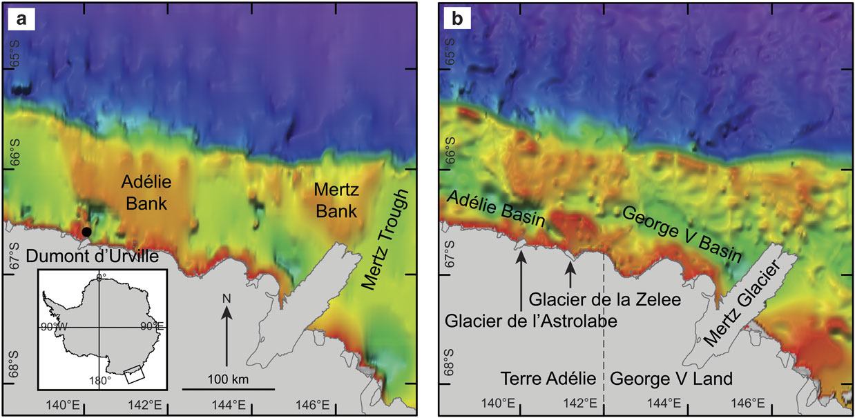
As a consequence of the frequent expeditions to the area, there is a higher density of digital bathymetric data available for the Terre Adélie and George V margin compared to other parts of East Antarctica. Two examples of previous bathymetric compilations into DEMs covering the area are the global GEBCO (IOC et al. 2003) and ETOPO1 (Amante & Eakins Reference Amante and Eakins2008) datasets (Fig. 1). The GEBCO grid is based upon depth contours derived from shiptrack soundings, while the ETOPO1 grid uses both shiptrack data and bathymetry derived from satellite altimetry (Smith & Sandwell Reference Smith and Sandwell1997). However, neither of these global grids provides sufficient spatial resolution at 1-arcminute (c. 1 mile) to assist in contemporary research programs, and both DEMs show considerable differences in the geomorphology of the shelf, mostly due to a lack of data coverage on the shelf. These deficiencies, and the availability of new shiptrack and multibeam depth data, have encouraged other efforts to develop regional-scale grids for the Terre Adélie and George V offshore region (e.g. Porter-Smith Reference Porter-Smith2003, Caburlotto et al. Reference Caburlotto, De Santis, Zanolla, Camerlenghi and Dix2006). However, these DEMs either lack the areal coverage or are not publicly available.
Mercator projection maps of a. GEBCO, and b. ETOPO1 bathymetry grids at 1-arcminute resolution (c. 1 mile), with the major physiographic features named on the Terre Adélie and George V shelves. The inset shows the study area on the East Antarctic margin. The hillshading angle and colour map used is identical to the hillshading angle and depth scale in Fig. 4. Coast and ice shelf boundaries were provided by the Australian Antarctic Division. Visual comparisons between the two grids show considerable differences in the morphology of the shelf.

This paper describes the development of a new high-resolution bathymetry model for the Terre Adélie and George V margin, called GVdem (short for George V digital elevation model). The GVdem grid spans an area 138–148°E, 63–69°S, with a cell pixel size of 0.001-arcdegree (c. 100 m). The total area of the GVdem grid is c. 302 000 km2, which also includes the land and ice sheet elevation coverage. Additional maps derived from the GVdem grid highlight seabed physiographic detail not previously observed for this part of East Antarctica, such as the complex inner-shelf valleys and their spatial relationship with large shelf depressions and the adjacent flat-topped banks. The new grid reveals further insight into the spatial distribution of the submarine canyons found on the continental slope. Together, these maps greatly improve the detail of the regional bathymetric setting, and provide fundamental spatial datasets for improving information on the physical environment of the region.
Methods
Multibeam data
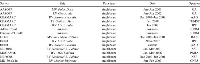
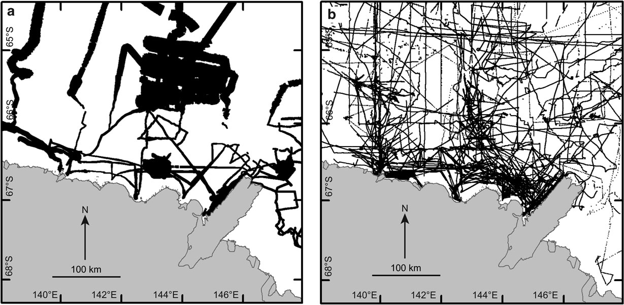
The various multibeam datasets (Table I, Fig. 2a) were originally processed with multibeam post-processing software, such as MBSystem (Caress & Chayes Reference Caress and Chayes1996) and Caris™ HIPS and SIPS, to correct for sound velocity variations within the water column and to remove noise. As far as we are aware, no account was taken of the tidal range during post-processing, so all data are assumed to have a vertical datum approximating mean sea level (MSL). All horizontal positions were referenced to the WGS84 datum. Our choice of 0.001-arcdegree (c. 100 m) cell pixel size in the final grid was because of the requirement to retain as high a level of detail in the geomorphology compared to the original multibeam data. The spatial resolution of multibeam is a function of the sonar beam angles in relation to water depth. As most of the multibeam systems used a 2° x 2° beam angle, which results in a seabed footprint of about 35 m in 1000 m depth, then 0.001-arcdegree was considered a good compromise between the resolutions of the various bathymetric data sources. The post-processed multibeam files were supplied to Geoscience Australia (GA) for archiving within HIPS and SIPS projects. For this project, the data were exported as ASCII xyz (longitude, latitude, depth) files for input to IVS 3D™ Fledermaus software for area based editing.
Summary of the singlebeam and multibeam source datasets used to create the GVdem gridFootnote a.

a GA = Geoscience Australia, IPF = Institut Polaire Francais, RAN = Royal Australian Navy, AAD = Australian Antarctic Division, TUMST = Tokyo University of Marine Science and Technology, SHOM = Service Hydrographique et Océanographique de la Marine, NSF = National Science Foundation, PNRA = Programma Nazionale di Ricerche in Antartide, CEAMARC = Collaborative East Antarctic Marine Census, AASOPP = Australian Antarctic and Southern Ocean Profiling Project, MOGAM = Morphology and Geology of Antarctic Margins, CNRS = Centre National de la Recherche Scientifique.
Mercator projection maps showing the spatial coverage of the a. multibeam, and b. singlebeam datasets used to develop the GVdem grid. Gridded xyz data from the SRTM30_Plus grid (Becker et al. Reference Becker, Sandwell, Smith, Braud, Binder, Depner, Fabre, Factor, Ingalls, Kim, Ladner, Marks, Nelson, Pharaoh, Trimmer, von Rosenberg, Wallace and Weatherall2009) were also used to provide additional data (c. 1 km resolution) to help fill in areas lacking multibeam and singlebeam coverage.

Singlebeam data
Singlebeam echosounder data from the numerous vessel transits and research voyages to the region were supplied to GA for archiving within Oracle spatial databases (Table I and Fig. 2b). In most cases, the shiptrack data were simply archived in ASCII xyz format with no further attribute data, therefore we assumed that no account was taken of the tides and so all sounding data were referenced to MSL. All depth data horizontal positions were referenced to the WGS84 datum. The spatial density of the shiptrack data reflected the pulse repetition frequency at the time of acquisition. So for shallower shelf waters, the depth sounding occurred at sub-second intervals, with the time period extending for deeper offshore waters. Thus data density were more densely clustered on the shelf compared to the offshore waters, but always at spatial densities < 100 m. Shiptrack data were extracted from the archive databases as individual ASCII xyz files for input to the Fledermaus area based editing software. In addition, we utilized gridded xyz data at c. 1 km resolution from the SRTM30_Plus grid (Becker et al. Reference Becker, Sandwell, Smith, Braud, Binder, Depner, Fabre, Factor, Ingalls, Kim, Ladner, Marks, Nelson, Pharaoh, Trimmer, von Rosenberg, Wallace and Weatherall2009) in order to help fill in areas lacking in either singlebeam or multibeam source data coverage.
Topography data
We utilized a clipped section of the Radarsat Antarctic Mapping Project (RAMP) Digital Elevation Model version 2 (Liu et al. Reference Liu, Jezek, Li and Zhao2001) for the land and ice sheet topography source data. The RAMP DEM combines topographic elevation data from a wide variety of cartographic, remotely sensed and survey data sources to provide a consistent coverage for all of Antarctica (http://nsidc.org/data/nsidc-0082.html, accessed February 2008). The RAMP DEM elevations were referenced to the OSU91A geoid, which approximates MSL, and therefore required no vertical adjustment in relation to the bathymetry data. The clipped RAMP DEM was reprojected and resampled using ESRI™ ArcGIS into an ESRI grid with geographic coordinates, using a horizontal datum of WGS84 and a cell pixel size of 0.0033-arcdegree (c. 333 m). The elevation data points were then extracted as ASCII xyz files for input to the Fledermaus area based editing process.
Coastline data
The Australian Antarctic Division (AAD) supplied an ArcGIS shapefile of the coastline, which included floating ice shelf boundaries and approximate grounding lines. A common problem when developing bathymetry models for Antarctica is where to draw the coastline, which effectively represents 0 m depth where the ice sheet meets the ocean. Deep ice shelf cavities typically underlie floating glacier tongues, and as the glaciers exclude ship-borne surveys, so the issue is how to model the ice shelf cavities with a lack of bathymetry data. Previous regional-scale DEMs have utilized BEDMAP (Lythe et al. Reference Lythe and Vaughan2000) data to provide data under floating ice shelves (e.g. Nitsche et al. Reference Nitsche, Jacobs, Larter and Gohl2007). In this project, we checked BEDMAP data against nearby shiptrack data collected in c. 1300 m adjacent to the Mertz Glacier Tongue, and found that the BEDMAP data underestimated the depths by nearly 1000 m. We therefore decided to reject BEDMAP data into the gridding process, and to select the grounding lines from the shapefile as the ice sheet/ocean boundary. Thus, the grounding line became the seaward boundary of the clipped RAMP DEM, and which allowed natural-looking cavities to develop beneath ice shelves and the nearest available bathymetry data during the interpolation process. The coastline shapefile was converted into an ESRI grid with a cell pixel size of 0.00025-arcdegree (c. 25 m), and then the node points were extracted to derive ASCII xyz files.
Grid development
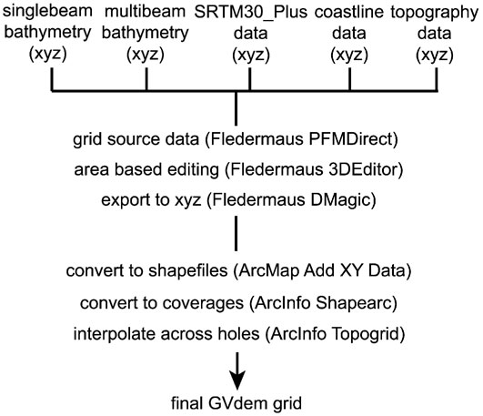
All singlebeam and multibeam bathymetry, SRTM30_Plus, coastline, and land topography xyz data were imported to Fledermaus PFMDirect software, which generated a gridded surface based upon the combined point data (Fig. 3). The PFM files could then be edited and cleaned of noise using the Fledermaus 3DEditor tool. 3DEditor makes it possible to edit the underlying data in a point cloud while dynamically updating the surface grid representation. The gridding method in PFMDirect utilized a weighted moving average with a weight diameter of three and a grid bin size of 100 m. As previously explained, this grid bin size was chosen as the highest resolution possible for the final grid and as a good compromise between the spatial resolutions of the various source datasets. Following extensive cleaning of the point cloud in 3DEditor, the result was an interim grid showing holes where no source point data existed. Another step was required to interpolate across the holes and complete the final GVdem grid. Fledermaus DMagic was used to export the interim grid node points as ASCII xyz files. These files were converted to point shapefiles using ArcMap. These shapefiles were converted to point coverages with ArcInfo Shapearc and then input to the ArcInfo Topogrid application (Hutchinson Reference Hutchinson1989) for interpolation across the holes into the final grid with a cell pixel size of 0.001-arcdegree. Two additional lower-resolution grids were also created at cell pixel sizes of 0.0025 (c. 250 m) and 0.005 (c. 500 m) -arcdegree, for users not requiring the highest resolution grid. The GVdem grid spans 138–148°E and 63–69°S, with an area of c. 302 000 km2 including the land elevation coverage.
The processing scheme used to combine the various bathymetry, coastline and land topography datasets into a gridded surface for area based editing, and then to interpolate across the data holes to develop the final GVdem grid.

Data statistics and accuracy
The development of the grid utilized over 27 million point soundings from the ship-borne surveys, of which about 97% of the bathymetric data were acquired using multibeam echosounders. In terms of data coverage, the initial source data represented between 30–40% of the total model area. However, the addition of the SRTM30_Plus grid data helped to fill in the remaining gaps where no data exists and reduced those gaps to less than c. 1 km during the final interpolation process. The source bathymetric data vertical and horizontal accuracies were classified according to the International Hydrographic Organization standards for hydrographic surveys Special Publication 44 (IHO 2008). The GVdem grid generally conforms to an Order 2 Total Horizontal Accuracy (THU) and Total Vertical Accuracy (TVU), based upon the worse case source data accuracy of Order 2. Both THU and TVU increase according to depth, so the maximum allowable THU is 30 m up to 100 m depth, 70 m up to 500 m depth, 120 m up to 1000 m depth, 220 m up to 2000 m depth, and so on. Realistically, however, the accuracy of GPS used for positioning during modern surveys is far better than the maximum allowable THU for Order 2 surveys, and so the THU figures quoted here are very conservative. The maximum allowable TVU for Order 2 surveys is 2.5 m up to 100 m depth, 11.5 m up to 500 m depth, 23 m up to 1000 m depth, 46 m up to 2000 m depth, and so on.
Derived maps
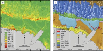
Following the development of the GVdem grid, a useful derived grid is a slope model which shows the angular variation in sea floor gradient relative to a horizontal or flat value of 0°. The 0.001-arcdegree grid was reprojected in ArcGIS to UTM54S, with a cell pixel size of 100 m. The slope model utilized the ArcInfo Slope tool by fitting a plane with a 3 x 3 cell neighbourhood around each processing or centre cell of the 100 m grid. Thus, slope was averaged over a distance of 300 m for each cell in order to derive a slope model. In addition, a map of the broad-scale geomorphic units was developed to highlight the boundaries of the main physiographic features. This map built upon previous geomorphic mapping conducted in the region (Beaman & Harris Reference Beaman and Harris2005). Using a combination of the 100 m slope grid, a hillshaded bathymetry grid, and a contour map at 100 m intervals, a line shapefile was hand drawn to delineate the geomorphic unit boundaries at a scale of 1:100 000. In addition, to highlight the positions of the axes of the submarine canyons incising the continental slope, a streamline analysis of the 0.001-arcdegree grid was conducted using ArcInfo. The analysis assumes equal ‘rainfall’ across the grid and then models the accumulation of water flow through the local basins. This resulted in line shapefiles representing streamlines showing the accurate positions of the axes from the major canyons and gullies on the continental slope and rise.
Results and discussion
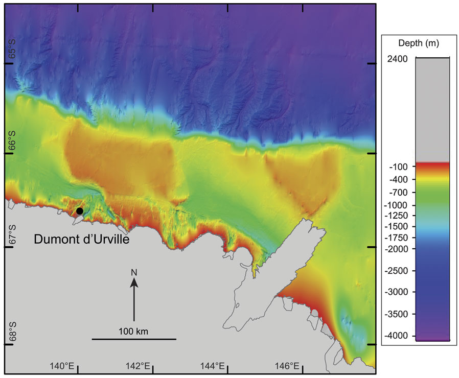
The new GVdem bathymetry model is shown in Fig. 4 and greatly improves the regional bathymetric setting of the Terre Adélie and George V margin compared to the GEBCO and ETOPO1 grids (see Fig. 1). In particular, the broader-scale complexity of the geomorphic features on the continental shelf are revealed, as well as more subtle and finer-scale physiographic features within the shelf depressions and inner-shelf valleys that reflect the palaeoglacial history of the area.
Mercator projection map of the new regional-scale bathymetry model, GVdem.

Continental shelf
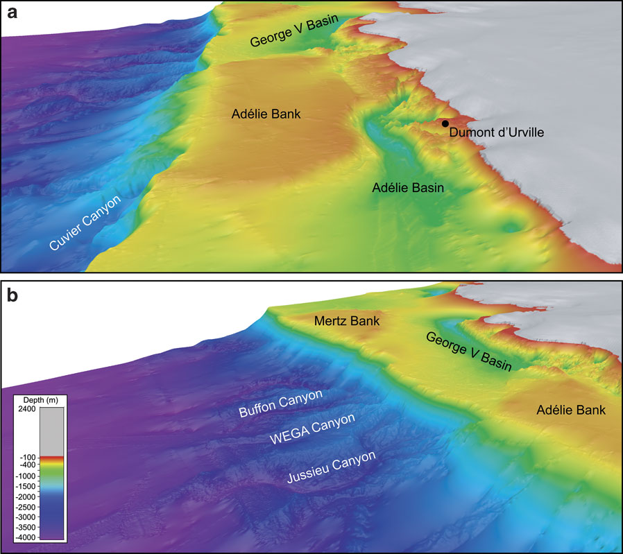
The shelf is dominated by the broad, relatively shallow (c. 200 m) Adélie and Mertz banks (Figs 5 & 6). These banks are remarkably flat and vary by only tens of metres across their entire extent. The banks are therefore similar to the smooth, planed bank tops found in other parts of the East Antarctic shelf (e.g. Harris & O’Brien Reference Harris and O’Brien1998). Both banks have a subtle concave surface towards their centres with maximum depths reaching c. 280 m. On the Adélie bank, this concave area connects to the south-east side of the bank and into the narrow rugged valleys of the inner-shelf. The Mertz bank has a well-defined, but not continuous, moraine feature that rims the landward edge of the bank, rising in places to about 120 m. It has previously been named the Mertz moraine and marks the edge of the glacial ice extent as it advanced across the shelf during the last glaciation (Domack et al. Reference Domack, Jull, Anderson, Linick and Williams1989, Beaman & Harris Reference Beaman and Harris2003). A similar discontinuous moraine feature appears as a series of low hills on the landward side of the Adélie bank adjacent to both the Adélie basin and George V basin. These hills rise to depths of about 130 m but do not extend as far north across the shelf as does the Mertz moraine. The moraines are currently sites for dense grounded bergs sourced from the Ross Ice Shelf, the Ninnis Glacier and the Cook Ice Shelf, and advected westwards via the westwind drift surface current (Massom Reference Massom2003). The Adélie and Mertz banks are separated by two relatively deep (> 1200 m) broad-scale, shelf depressions: the Adélie basin (also called the Dumont d’Urville basin) and the George V basin (also called the Adélie depression or Mertz-Ninnis trough). Note that the extent of the large shelf depression lying to the east of the Mertz Glacier at 147°E is still largely unknown due to the paucity of depth data in the area. Wide cross-shelf valleys, such as the Mertz trough (see Fig. 1 for location), connect these depressions to the shelf edge, forming sills on the outer-shelf in depths ranging between c. 420–500 m. Glacial megaflute features up to 10 m high can be traced for c. 100 km along the bottom of the George V basin, which then follows the northerly turn of the cross-shelf valley towards the sill near the shelf break (Beaman & Harris Reference Beaman and Harris2005). Megaflute features are also observed in the Adélie basin where limited multibeam data have been collected but their northerly extent across the shelf is not obvious. Several grounding-line wedges lie within the Mertz trough on the outer-shelf. These wedges have previously been studied for erosional features caused by subglacial meltwater breaching the deposits, and as further evidence that an ice sheet once covered the depressions during glacial maximal conditions (McMullen et al. Reference McMullen, Domack, Leventer, Olsen, Dunbar and Brachfield2006). For the first time, the extent and complexity of the inner-shelf valleys are revealed which dominate about a third of the width of the shelf and are located wherever bathymetry data were available near the coast (Fig. 5a). As the inner-shelf is the least surveyed area, the spatial extent of these steep valleys are probably much greater than presently shown in the GVdem grid, particularly to the east of the Mertz Glacier where there are a lack of bathymetric survey data. The inner-shelf valleys may plunge to depths of 1200 m over distances of only several kilometres north of the coastline to form relatively small enclosed basins. These small basins then connect to the larger Adélie and George V basins via narrow rugged canyons, which may trend in varying directions across the inner-shelf and even parallel to the coast. Several floating glacier tongues, such as the Glacier de l’Astrolabe and Glacier de la Zelee (see Fig. 1 for location), feed directly into the heads of these valleys. However, adjacent to other deep inner-shelf valleys no such glacier tongue is obvious. The extensive nature of the inner-shelf valleys and canyons points to a wider advancement of the continental ice sheet beyond the major glacial drainage areas during glacial maxima periods.
3D oblique views of the GVdem grid showing a. easterly-looking view of the complex inner-shelf valleys and flat-topped banks, and b. south-easterly-looking view of the continental slope submarine canyons and adjacent abyssal plain.

Mercator projection maps of a. the slope gradient in degrees, and b. the broad-scale geomorphic units together with streamlines marking the submarine canyon axes. The maps highlight the steeper inner-shelf valleys and slope canyons versus the flat-topped shelf banks and relatively smooth shelf depressions.

Continental slope and abyssal plain
The shelf break depths vary between about 500 m north of the Adélie and Mertz banks, to slightly deeper depths of up to 660 m where the broad cross-shelf valleys form sills on the outer-shelf, such as where the Adélie basin connects to the shelf edge. Within the upper slope zone between about 500–2000 m, the gradually sloping seabed initially appears relatively smooth down to depths of 1000 m. Deeper than about 1000 m, large submarine canyons have incised into the continental slope, together with small gullies that form dendritic canyon heads. Numerous small gullies also cover the canyon walls that converge with the main canyon axes in depths below about 2000 m within the lower slope zone. Some of the larger canyons north of the George V basin have been named the Buffon, WEGA and Jussieu Canyons (Fig. 5b), and are well studied for their palaeoglacial signatures (e.g. De Santis et al. Reference De Santis, Brancolini and Donda2003, unpublished data, Donda et al. Reference Donda, Brancolini, de Santis and Trincardi2003). Several canyon heads are the locations of dense coral-sponge communities, such as the Cuvier and Jussieu canyons (Post et al. Reference Post, O’Brien, Beaman, Riddle and de Santis2010). The submarine canyon axes generally drain northward from the margin, and are separated by steep parallel ridges that rise about 200 m above the axes. Eventually the canyons and ridges start to merge into the relatively flat abyssal plain below about 3500 m depth, which deepens to about 4000 m at the northern limit of the bathymetry model.
Conclusion
We have described the development of a new high-resolution bathymetry model for the Terre Adélie and George V continental margin, called GVdem. The GVdem grid spans an area 138–148°E and 63–69°S, with a cell pixel size of 0.001-arcdegree (c. 100 m). The total area of GVdem is about 302 000 km2, which also includes the land and ice sheet elevation coverage.
The revised depth model is a large improvement over previously available regional-scale DEMs, and highlights seabed physiographic detail not formerly observed in this part of East Antarctica. In particular, the extent and complexity of the inner-shelf valleys are revealed and their relationship with large shelf basins and adjacent flat-topped banks. The new grid also reveals further insight into the spatial distribution of the submarine canyons found on the continental slope.
The GVdem grid may be downloaded in a choice of ESRI ASCII raster files and as hillshaded geotifs, via the Catalogue of Australian Antarctic and Subantarctic Metadata (CAASM) under the title: a bathymetric Digital Elevation Model (DEM) of the George V and Terre Adélie continental shelf and margin. http://gcmd.nasa.gov/KeywordSearch/Home.do?Portal=amd_au&MetadataType=0. [Dataset Text Search = GVdem_2008].
Acknowledgments
We thank the numerous agencies responsible for collecting the source bathymetry data over many years, in particular the Service Hydrographique et Océanographique de la Marine, National Science Foundation, Programma Nazionale di Ricerche in Antartide, and Australian Antarctic Division. Mike Sexton at Geoscience Australia provided much assistance in compiling the various datasets for this project. Robin Beaman acknowledges the research salary support by the Reef and Rainforest Research Centre and a Queensland Government Smart Futures Fellowship. We acknowledge the assistance of Frank Nitsche, Peter Fretwell, and two anonymous Geoscience Australia reviewers for their thorough reviews and constructive criticisms of the manuscript. Phil O’Brien and Alexandra Post publish with permission of the Chief Executive Officer, Geoscience Australia.