1 Introduction
Capillary-dominated fluid behaviour is common over large length scales in the near-weightless environment aboard spacecraft. In part due to both the expense and limited opportunities for designers to develop significant intuition of general multiphase phenomena in such environments, developing robust fluid systems for spacecraft fuels management, thermal control and water processing for life support remains challenging. As examples, it is not uncommon for life support equipment function to be hampered by unanticipated bubble occlusions, wetting transitions, wicking migrations and capillary surface instabilities leading to undesirable interface topologies. Though largely unpublished in the scientific literature, such occurrences can be learned from the space news media. A poignant example of bubbles shutting down a primary oxygen production system aboard the International Space Station (ISS) provides a case in point as reported by Oberg (Reference Oberg2006), highlighting the need to develop further insights and tools such that advanced fluid system design can proceed with expectations of greater reliability.
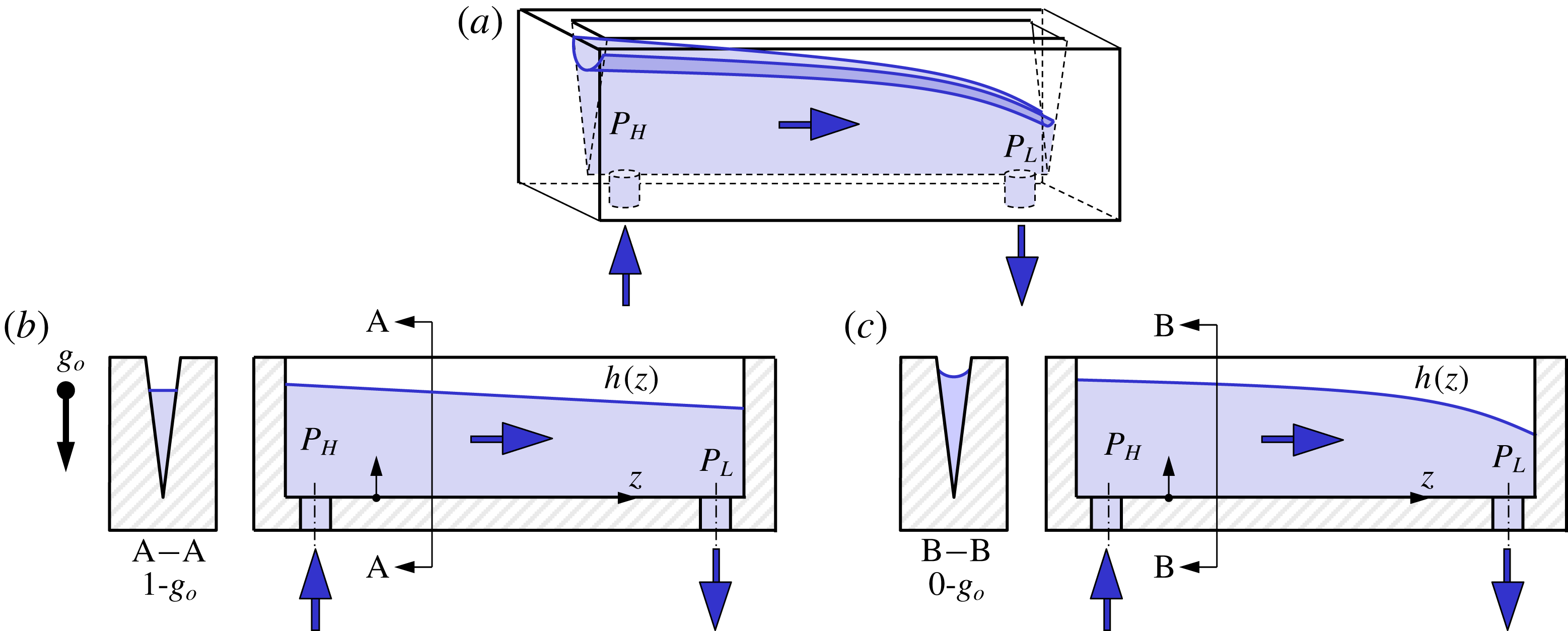
Due to the effectively zero-gravity conditions of orbiting spacecraft, there is fundamentally no up or down, and the terrestrial expectations of a ‘bottom’ for multiphase flow phenomena must be suspended. Fortunately, in certain cases, the normally ubiquitous and often beneficial passive role of gravity may be replaced in the weightless environment by the equally passive combined effects of surface tension, wetting and system geometry. As a simple example, in figure 1 we sketch an open triangular channel (also known as groove, trough, wedge, etc.) partially filled with liquid. The liquid is pumped into the lower left port and removed from the lower right port. In figure 1(b), though the steady liquid flow rate is delivered to the channel by a pump, gravity drives the liquid from left to right across the open channel via hydrostatic pressure forces, since pressures
 $P_{H}>P_{L}$
owing to the downward gravity vector. In figure 1(c), the same steady flow rate is transported, but in the absence of gravity the flow is driven by a capillary under-pressure gradient caused by the height profile
 $h(z)$
of the meniscus along the channel – the capillary pressure in the liquid becoming increasingly negative the shallower the liquid in the channel (Melin, van der Wijngaart & Stemme Reference Melin, van der Wijngaart and Stemme2005; Klatte et al.
Reference Klatte, Haake, Weislogel and Dreyer2008; Ramé & Weislogel Reference Ramé and Weislogel2009). The two flows appear similar and a useful degree of passive control is established in figure 1(c) despite the absence of gravity. The fact that large length scale stable capillary systems can be exploited in low-gravity environments means that significantly larger flow velocities and flow rates may be achieved, establishing capillary solutions as attractive options for spacecraft fluid systems design.
(a) Perspective sketch of horizontal open-wedge channel identifying pump inlet and outlet steady flow rates (arrows). (b) Gravity-dominated interface profile with section A–A. (c) Low-
 $g$
surface tension-dominated interface profile with section B–B. Identical flow rates and similar interface profiles are established with the role of gravity in (b) replaced by the combined effects of surface tension, geometry and wetting in (c).

Terrestrial investigations concerning the interior corner flow geometry in figure 1(c) are numerous, including a host of wicking, droplet and bubble migration flows. Terrestrial applications and experimental verifications are limited by the size of the system through the Bond number
 $Bo\equiv \unicode[STIX]{x1D70C}gR^{2}/\unicode[STIX]{x1D70E}\ll 1$
and capillary length
 $H_{c}\sim \unicode[STIX]{x1D70E}/\unicode[STIX]{x1D70C}gL$
, determined by a balance of capillary and hydrostatic pressures, where
 $R$
is a characteristic length of the interface,
 $\unicode[STIX]{x1D70E}$
the surface tension,
 $\unicode[STIX]{x1D70C}$
the density difference across the interface and
 $g$
the local acceleration field strength (i.e. gravity). Parameter
 $L$
is the vertical length scale, and for horizontal flows and flows with only one length scale,
 $L\approx H_{c}$
, such that
 $H_{c}\sim (\unicode[STIX]{x1D70E}/\unicode[STIX]{x1D70C}g)^{1/2}$
is the well-established capillary height.
On Earth, for typical liquids
 $H_{c}\lesssim O(1~\text{mm})$
. For the interior corner capillary flow geometry, Dong & Chatzis (Reference Dong and Chatzis1995), Romero & Yost (Reference Romero and Yost1996) and others provide early solutions relating to transient constant pressure wicking flows in the visco-capillary limit. Ransohoff & Radke (Reference Ransohoff and Radke1988) make application to snap-off phenomena in multiphase flows, Khare et al. (Reference Khare, Brinkmann, Bruce, Law, Gurevich, Herminghaus and Seemann2007) demonstrate edge wetting and de-wetting transitions by applying electrical fields and Ponomarenko, Clanet & Quéré (Reference Ponomarenko, Clanet and Quéré2011) provide a long-time universal scaling law for capillary rise. Gravity draining in such geometries is pursued by Bico & Quéré (Reference Bico and Quéré2002) and the migration of bubbles and drops in wedges is demonstrated and investigated by Litterst et al. (Reference Litterst, Eccarius, Hebling, Zengerle and Koltay2006), Metz et al. (Reference Metz, Paust, Zengerle and Koltay2012), Dangla, Kayi & Baroud (Reference Dangla, Kayi and Baroud2013), Reyssat (Reference Reyssat2014) and others. The effects of rounded corners are included by Dong & Chatzis (Reference Dong and Chatzis1995) and Chen, Weislogel & Nardin (Reference Chen, Weislogel and Nardin2006), along with the effects of variably wetted corners by Weislogel & Nardin (Reference Weislogel and Nardin2005), non-planar corners by Weislogel (Reference Weislogel2001) and Ponomarenko et al. (Reference Ponomarenko, Clanet and Quéré2011) and non-wetting liquids by Bolleddula & Weislogel (Reference Bolleddula and Weislogel2009). The corner wetting condition is attributed to Concus & Finn (Reference Concus and Finn1969), with pinning effects originally pursued by Romero & Yost (Reference Romero and Yost1996), and non-wetted corner stability by Langbein (Reference Langbein1990). Analytical methods addressing coordinate transformations (i.e. Stocker & Hosoi Reference Stocker and Hosoi2005) and slender visco-capillary-gravity flows of more general section are expanded by Bowen & King (Reference Bowen and King2013) (see also references contained therein).
The larger length scale flows in low-gravity environments provide avenues for greater inertia. The capillary channel flow experiments conducted on the ISS demonstrate forced visco-inertial capillary flows exploiting the open-wedge geometry for enhanced stability and passive bubble separations (Jenson et al.
Reference Jenson, Wollman, Weislogel, Sharp, Green, Canfield, Klatte and Dreyer2014). The capillary flow experiments (CFE), also performed aboard the ISS, provide data benchmarks for larger bubble migration flows controlled primarily by interconnected interior corners – so-called ‘compound capillary flows’ (Weislogel et al.
Reference Weislogel, Chen, Collicott, Bunnell, Green and Bohman2009; Weislogel, Baker & Jenson Reference Weislogel, Baker and Jenson2011; Weislogel Reference Weislogel2012). The most controlled experiments employ perfectly wetting liquids, but in the interest of applications circulating contaminated water streams aboard spacecraft, partial wetting systems with large contact angle hysteresis have become a focus with recent demonstrations on the ISS exploiting the open-wedge geometry for direct contact liquid sorbents in
 $\text{CO}_{2}$
scrubbing applications (Viestenz, Weislogel & Sargusingh Reference Viestenz, Weislogel and Sargusingh2018). In many cases, however, despite the larger dimensions of low-gravity capillary flows, the increasingly slender nature of the interior corner flow geometry inevitably recovers the nearly parallel visco-capillary flow balance. This is in part due to the fact that in microgravity environments, for centimetric diameter conduits, interior corner capillary flow lengths are many metres, establishing slenderness ratios comparable to terrestrial microfluidic investigations. Nonetheless, low-gravity capillary fluidics research is unique in the durations and rates by which the often transient capillary-driven flows pass through unsteady, convective, diffusive and ultimately diffusive-acceleration regimes (Fries & Dreyer Reference Fries and Dreyer2008; Ponomarenko et al.
Reference Ponomarenko, Clanet and Quéré2011).
Despite works that successfully address ample inertia in otherwise visco-capillary flows (e.g. Quéré Reference Quéré1997, Reference Quéré1999, Rosendahl, Ohlhoff & Dreyer Reference Rosendahl, Ohlhoff and Dreyer2004, Fries & Dreyer Reference Fries and Dreyer2008), inclusion of small inertia from a theoretical perspective continues to present challenges, even in situations where
 $O$
(1) solutions are exact (i.e. the spreading drop problem; Weislogel & Lichter Reference Weislogel and Lichter1996). Despite persistent difficulties specifying moving contact line boundary conditions, numerical methods meet with better success when considering inertia and greater geometric complexity. As examples for interior corner flows, numerical investigations by Wang et al. (Reference Wang, Xu, Sun and Hu2010), Li & Liu (Reference Li and Liu2014) and Wu et al. (Reference Wu, Huang, Chen and Zhang2018) add geometry, time-varying capillary pressure boundary conditions and corner curvature computations for the corner rise problem.
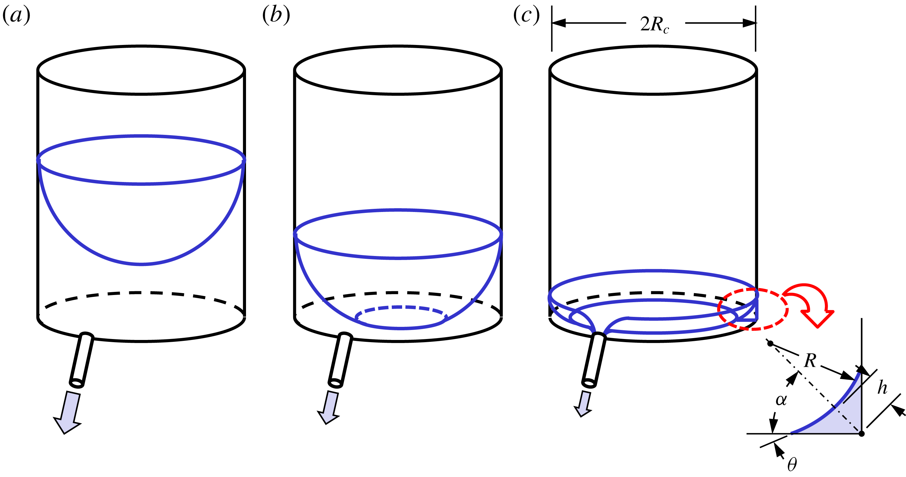
Depiction of zero-gravity draining from a right circular cylinder with planar base: (a) bulk draining, (b) begin three-dimensional corner flows and (c) late-stage predominately one-dimensional corner flow draining analysed herein.

Due to both simplicity and passivity, devices for fluid management aboard spacecraft often exploit the interior corner geometry to drive liquids along desired paths (Jaekle Reference Jaekle1991; Chato & Martin Reference Chato and Martin2006). The spacecraft application problems listed and literature reviewed in Weislogel (Reference Weislogel2003) remain pertinent in this regard. It is often our experience that increased computational capabilities do not always accompany decreasing run times, placing a premium on analytical approximations that can be used as most efficient guides for the fewest numerical runs.
In the present work we add an exact solution for the late-stage forced draining of certain interior corner geometries partially filled with wetting liquids. A pertinent application problem is sketched in figure 2, where a right circular cylinder is slowly drained in a low-gravity environment. As the liquid level decreases, a dry circular region forms on the base forming a continuous capillary filament along the interior corner created by the circular base and the cylindrical sidewalls (figure 2 b,c). It is the late-stage draining of the interior corner flow topology in figure 2(c) that is of interest here, as such transient flows can be critical for the withdrawal of precious fuels, propellants, coolants or biofluids during lab-on-chip processing. A single drain location is depicted in figure 2. We begin our analysis by assuming a single linear interior corner with two identical drain locations hereafter referred to as the ‘double-drain problem’. It will be shown that the formulation leads to numerical solutions which are nearly coincident with second-order accurate asymptotic approximations. The solution is then discussed in the context of other corner flow solutions before being compared to experimental results collected in space and on Earth. With favourable agreement the theory is extended to possible application problems where knowledge of liquid configurations, volumes and drain rates is critical to system design.
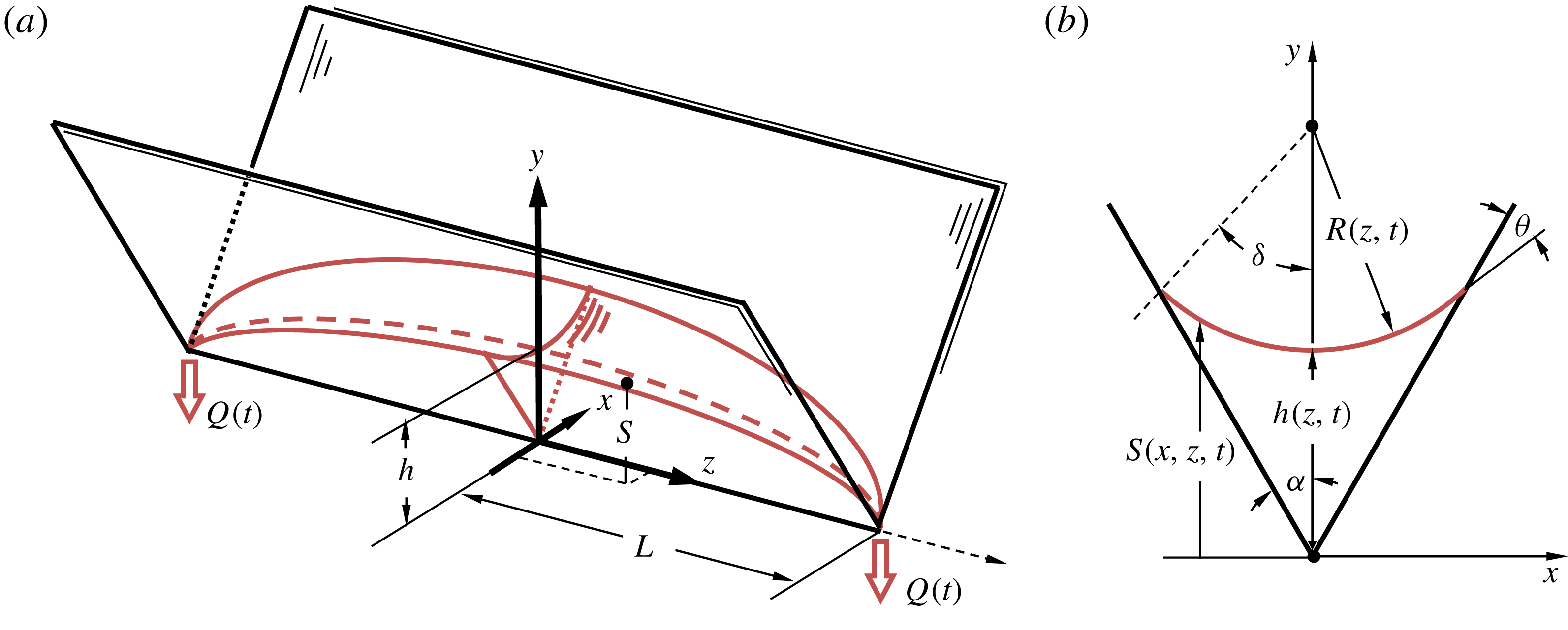
Schematic of double-drained wetting capillary liquid in an interior corner. The draining locations are symmetric at
 $z=\pm L$
at volumetric sink flow rates
 $Q$
: (a) perspective view and (b) section view with notation employed in solution. Here
 $S(x=0,z,t)\equiv h(z,t)$
is the meniscus centreline profile.

2 Formulation and numerical solution
A double-drained interior corner capillary flow is sketched in figure 3 with critical dimensions noted. It is assumed the liquid is drained symmetrically and identically with volumetric flow rate
 $Q(t)$
at
 $z=\pm L$
, where the centreline meniscus elevation
 $h(\pm L,t)=0$
. As liquid is removed at the drain location(s), the local meniscus height
 $h(z,t)$
decreases. As a consequence, the capillary pressure becomes increasingly negative via
 $P(z,t)\sim -1/h$
, which drives liquid from deeper regions to shallower ones. For this geometry the total drain rate is
 $Q_{tot}=2Q$
. Gravity is negligible and
 $V(t)$
is the half-volume of the liquid at time
 $t$
.
We briefly summarize the development of the governing equation here. Following the notation of Weislogel & Lichter (Reference Weislogel and Lichter1998), neglecting the influence of the surrounding gas and thin-film effects associated with finite surface roughness and van der Waals forces, the lubrication analysis assumes the constraints of a slender column, negligible streamwise free surface curvature and negligible inertia, where respectively
 $$\begin{eqnarray}\unicode[STIX]{x1D716}^{2}\equiv \left(\frac{H}{L}\right)^{2}\ll 1,\quad \unicode[STIX]{x1D716}^{2}f\ll 1,\quad \frac{\unicode[STIX]{x1D716}^{2}SuF_{i}^{2}\sin ^{4}\unicode[STIX]{x1D6FC}}{f}\ll 1,\end{eqnarray}$$
with
 $$\begin{eqnarray}f=\frac{\sin \unicode[STIX]{x1D6FC}}{\cos \unicode[STIX]{x1D703}-\sin \unicode[STIX]{x1D6FC}},\end{eqnarray}$$
which is a dimensionless geometric cross-stream free surface radius of curvature function. Angle
 $\unicode[STIX]{x1D6FC}$
is the interior corner half-angle,
 $\unicode[STIX]{x1D703}\leqslant \unicode[STIX]{x03C0}/2-\unicode[STIX]{x1D6FC}$
is the wetting angle satisfying the Concus–Finn corner wetting condition (Concus & Finn Reference Concus and Finn1969),
 $Su\equiv \unicode[STIX]{x1D70C}\unicode[STIX]{x1D70E}H/\unicode[STIX]{x1D707}^{2}$
is the Suratman number (a Reynolds number with capillary velocity scale
 $\unicode[STIX]{x1D70E}/\unicode[STIX]{x1D707}$
),
 $\unicode[STIX]{x1D70C}$
,
 $\unicode[STIX]{x1D70E}$
and
 $\unicode[STIX]{x1D707}$
are the fluid density, surface tension and dynamic viscosity, and
 $H$
is the characteristic meniscus height. Under these conditions the three-dimensional free surface
 $S(y,z,t)$
may be characterized in terms of the
 $y$
–
 $z$
-plane geometry identified by
 $h=h(z,t)$
and the cross-flow radius of curvature
 $R=fh$
in figure 3:
 $$\begin{eqnarray}S=h(1+f)-fh\left(1-\left(\frac{y\tan \unicode[STIX]{x1D6FC}}{fh}\right)^{2}\right)^{1/2}.\end{eqnarray}$$
In the manner of Ransohoff & Radke (Reference Ransohoff and Radke1988), Dong & Chatzis (Reference Dong and Chatzis1995), Romero & Yost (Reference Romero and Yost1996), Weislogel & Lichter (Reference Weislogel and Lichter1998), Langbein (Reference Langbein2002) and others, employing subscript notation for partial differentiation, the mass conservation equation for this incompressible flow is
 $$\begin{eqnarray}A_{t}=-Q_{z},\end{eqnarray}$$
where
 $A$
is the
 $x$
–
 $y$
-plane cross-sectional area and
 $Q$
is the
 $z$
-direction flow rate. It is similarly shown in Weislogel & Lichter (Reference Weislogel and Lichter1998) that
 $$\begin{eqnarray}A=F_{A}h^{2},\quad Q=-\frac{WAL}{H}~h_{z},\quad F_{A}=f^{2}\left(\frac{\cos \unicode[STIX]{x1D703}\sin \unicode[STIX]{x1D6FF}}{\sin \unicode[STIX]{x1D6FC}}-\unicode[STIX]{x1D6FF}\right),\quad W=\frac{\unicode[STIX]{x1D70E}}{\unicode[STIX]{x1D707}}\frac{H}{L}\frac{F_{i}\sin ^{2}\unicode[STIX]{x1D6FC}}{f},\end{eqnarray}$$
where
 $\unicode[STIX]{x1D6FF}=\unicode[STIX]{x03C0}/2-\unicode[STIX]{x1D6FC}-\unicode[STIX]{x1D703}$
is the section curvature angle and
 $1/8\lesssim F_{i}(\unicode[STIX]{x1D6FC},\unicode[STIX]{x1D703})\leqslant 1/6$
is a numerically determined inverse viscous resistance coefficient that renders the velocity scale
 $W$
and assessment of inertia (third constraint (2.1)) more quantitative. Substitution of (2.5) into (2.4) yields the governing evolution equation for the half-domain
 $$\begin{eqnarray}(h^{2})_{t}=\frac{WL}{H}(h^{2}h_{z})_{z},\end{eqnarray}$$
subject to boundary conditions
 $h_{z}(0,t)=0$
,
 $h(L,t)=0$
, and initial half-domain volume condition
 $$\begin{eqnarray}V_{i}\equiv V(0)=\int _{0}^{L}F_{A}(h(z,0))^{2}\,\text{d}z.\end{eqnarray}$$
Equations (2.6) and (2.7) suggest non-dimensionalizations
 $z^{\ast }=z/L$
,
 $h^{\ast }=h/H\equiv h/\left(V_{i}/F_{A}L\right)^{1/2}$
and
 $t^{\ast }=W(t-t_{o})/L$
, where now
 $t\geqslant t_{o}$
in anticipation of experimental offset or start-up time
 $t_{o}$
. Equation (2.6) can then be non-dimensionalized to find
 $$\begin{eqnarray}\left(h^{\ast 2}\right)_{t^{\ast }}={\textstyle \frac{1}{3}}(h^{\ast 3})_{z^{\ast }\!z^{\ast }},\end{eqnarray}$$
subject to
 $h_{z^{\ast }}^{\ast }=0$
at
 $z^{\ast }=0$
,
 $h^{\ast }=0$
at
 $z^{\ast }=1$
, and
 $$\begin{eqnarray}1=\int _{0}^{1}\left(h^{\ast }(z^{\ast },0)\right)^{2}\,\text{d}z^{\ast },\end{eqnarray}$$
where superscript
 $^{\ast }$
denotes a dimensionless quantity. Equations (2.8)–(2.9) and boundary conditions represent the governing system for the double-drain problem.
For
 $z^{\ast }\sim O(1)$
, equation (2.8) implies
 $h^{\ast }\sim t^{\ast -1}$
, which suggests a separation of variables solution of the form
 $$\begin{eqnarray}h^{\ast }(z^{\ast },t^{\ast })=\frac{F(z^{\ast })}{\left(t_{i}^{\ast }+t^{\ast }\right)},\end{eqnarray}$$
which when substituted into (2.8) yields
 $$\begin{eqnarray}\left(F^{3}\right)^{\prime \prime }+6F^{2}=0,\end{eqnarray}$$
subject now to
 $F^{\prime }(0)=0$
,
 $F(1)=0$
, and
 $$\begin{eqnarray}t_{i}^{\ast 2}=\int _{0}^{1}F^{2}\,\text{d}z^{\ast }.\end{eqnarray}$$
Quantity
 $t_{i}^{\ast 2}$
is a constant representing the dimensionless initial volume condition of (2.10) at
 $t^{\ast }=0$
following substitution into (2.9). Primes denote ordinary differentiation with respect to
 $z^{\ast }$
. The substitution
 $U=F^{3}$
into (2.11) avoids a singularity at
 $z^{\ast }=1$
and yields the further transformed nonlinear equation
 $$\begin{eqnarray}U^{\prime \prime }+6U^{2/3}=0,\end{eqnarray}$$
subject to
 $U^{\prime }(0)=0$
and
 $U(1)=0$
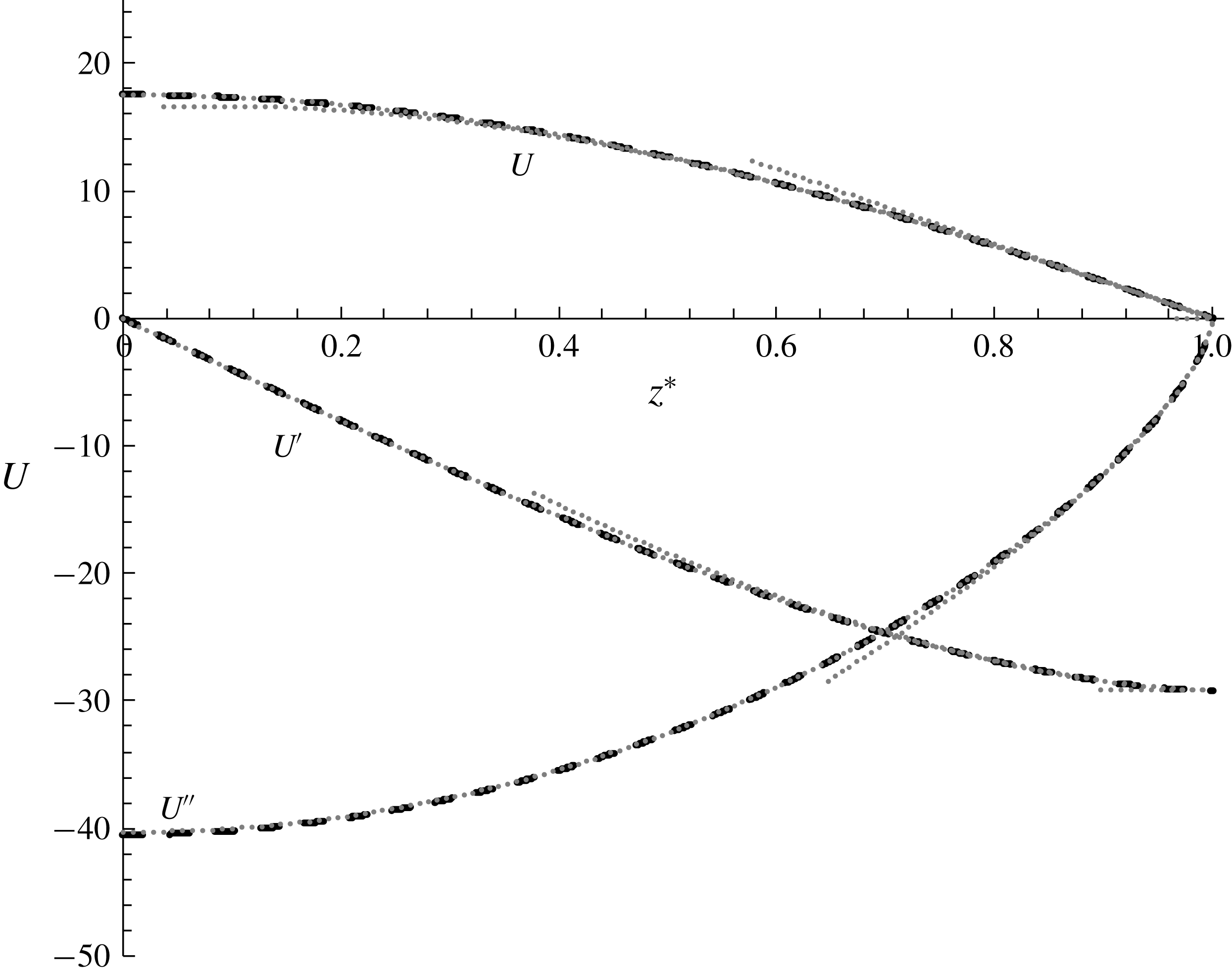
. Equation (2.13) is solved numerically and presented in figure 4. Useful limiting numerical values are
 $U(0)\approx 17.538$
,
 $U^{\prime }(1)\approx -29.195$
,
 $U^{\prime \prime }(0)\approx -40.501$
and
 $U^{\prime \prime }(1)\approx 0$
. Equation (2.12) is then solved to find
 $$\begin{eqnarray}t_{i}^{\ast }\approx 2.20588.\end{eqnarray}$$
To evaluate (2.10),
 $F=U^{1/3}$
may be computed, where unbounded slope and curvature are observed as
 $z^{\ast }\rightarrow 1$
.
Numerical solutions for
 $U(z^{\ast })$
from (2.13) from which
 $F(z^{\ast })=U^{1/3}$
. Zeroth-, first- and second-order asymptotic approximations are shown using truncated grey dotted lines for
 $U$
,
 $U^{\prime }$
and
 $U^{\prime \prime }$
. The second-order approximation is visually coincident with the numerical solutions for
 $0\leqslant z^{\ast }\leqslant 1$
.

At
 $z^{\ast }=1$
, the dimensionless flow rate
 $Q^{\ast }\equiv QL/WV_{i}$
is
 $$\begin{eqnarray}Q^{\ast }(1,\hat{t}^{\ast })=-\frac{U^{\prime }(1)}{3t_{i}^{\ast 3}}\frac{1}{(1+\hat{t}^{\ast })^{3}}\approx \frac{0.907}{(1+\hat{t}^{\ast })^{3}},\end{eqnarray}$$
where
 $-U^{\prime }(1)/3t_{i}^{\ast 3}=68/75\approx 0.907$
and
 $\hat{t}^{\ast }\equiv t^{\ast }/t_{i}^{\ast }$
. The liquid fill fraction
 $V^{\ast }\equiv V/V_{i}$
within the half-domain
 $0\leqslant z^{\ast }\leqslant 1$
may be computed using (2.15), noting that
 $-U^{\prime }(1)/6t_{i}^{\ast 2}=1$
, to find
 $$\begin{eqnarray}V^{\ast }=1-t_{i}^{\ast }\int _{0}^{t^{\ast }}Q^{\ast }\,\text{d}\hat{t}^{\ast }\approx \frac{1}{(1+\hat{t}^{\ast })^{2}}.\end{eqnarray}$$
At
 $z^{\ast }=0$
,
 $$\begin{eqnarray}h^{\ast }(0,\hat{t}^{\ast })=\frac{(U(0))^{1/3}}{t_{i}^{\ast }}\frac{1}{(1+\hat{t}^{\ast })}\approx \frac{1.178}{(1+\hat{t}^{\ast })}.\end{eqnarray}$$
Thus, from (2.17), (2.16) and (2.15), at long times
 $h^{\ast }\sim t^{\ast -1}$
,
 $V^{\ast }\sim t^{\ast -2}$
and
 $Q^{\ast }\sim t^{\ast -3}$
.
The constraints of (2.1) are assessed in light of the solution to find the slenderness criterion
 $$\begin{eqnarray}\unicode[STIX]{x1D716}^{2}\sim h_{z}^{2}=\left(\frac{H}{L}\right)^{2}\left(h_{z^{\ast }}^{\ast }\right)^{2}=\left(\frac{H}{L}\right)^{2}\frac{F^{\prime 2}}{t_{i}^{\ast 2}\left(1+\hat{t}^{\ast }\right)^{2}}=\frac{1}{9t_{i}^{\ast 2}}\frac{V_{i}}{F_{A}L^{3}}\frac{U^{-4/3}U^{\prime 2}}{\left(1+\hat{t}^{\ast }\right)^{2}}\ll 1.\end{eqnarray}$$
This relationship is difficult to satisfy for finite time since
 $U(z^{\ast }\rightarrow 1)\rightarrow 0$
.
In the vicinity of the drain location an approximate linear solution is
 $$\begin{eqnarray}U(z^{\ast }\rightarrow 1)\approx -U^{\prime }(1)(1-z^{\ast })\end{eqnarray}$$
from which
 $$\begin{eqnarray}F(z^{\ast }\rightarrow 1)\approx \left(-U^{\prime }(1)\right)^{1/3}(1-z^{\ast })^{1/3}.\end{eqnarray}$$
The zeroth-order asymptotic limit of (2.19) is added to figure 4 which establishes reasonable agreement for
 $z^{\ast }\gtrsim 0.75$
. Since the slender column (shallow slope) constraint of (2.18) is problematic for
 $z^{\ast }\rightarrow 1$
, equation (2.19) is substituted into (2.18) to find
 $$\begin{eqnarray}\unicode[STIX]{x1D716}^{2}\sim h_{z}^{2}=\frac{(-U^{\prime }(1))^{2/3}}{9t_{i}^{\ast 2}}\frac{V_{i}}{F_{A}L^{3}}\frac{1}{\left(1+\hat{t}^{\ast }\right)^{2}}\frac{1}{(1-z^{\ast })^{4/3}}\ll 1.\end{eqnarray}$$
For fixed
 $\hat{t}^{\ast }$
the solution fails as
 $z^{\ast }\rightarrow 1$
. However, when
 $\hat{t}^{\ast }\gg 1$
, equation (2.21) suggests the solution is appropriate for
 $V_{i}/F_{A}L^{3}\ll 1$
and
 $0\leqslant z^{\ast }\lesssim 1-\hat{t}^{\ast -3/2}$
. The other constraints of (2.1) are found similarly:
 $\unicode[STIX]{x1D716}^{2}f\sim fV_{i}/F_{A}L^{3}\ll 1$
and
 $\unicode[STIX]{x1D716}^{2}SuF_{i}^{2}\sin ^{4}\unicode[STIX]{x1D6FC}/f\sim V_{i}SuF_{i}^{2}\sin ^{4}\unicode[STIX]{x1D6FC}/fF_{A}L^{3}\ll 1$
, also for
 $0\leqslant z^{\ast }\lesssim 1-\hat{t}^{\ast -3/2}$
.
3 Drain location asymptotics,
 $1-z^{\ast }\ll 1$

By inspection of (2.13), and as confirmed from the numerical results, for
 $z^{\ast }\rightarrow 1$
,
 $U(z^{\ast })\rightarrow 0$
such that
 $U^{\prime \prime }(z^{\ast })\rightarrow 0$
from which we gather
 $U^{\prime }(z^{\ast })\rightarrow \text{const}$
. Thus, by assuming
 $U(1)=0$
and
 $U^{\prime }(0)=\text{const.}$
, an asymptotic solution for
 $U(z^{\ast }\rightarrow 1)$
may be pursued by introducing the transform
 $\unicode[STIX]{x1D719}^{1/2}\unicode[STIX]{x1D709}=1-z^{\ast }$
, where
 $0<\unicode[STIX]{x1D719}$
is a dummy gauge function initially assumed small, and
 $\unicode[STIX]{x1D709}$
is an
 $O(1)$
dimensionless drain location coordinate. Transforming (2.13)
 $z^{\ast }\mapsto \unicode[STIX]{x1D709}$
yields
 $$\begin{eqnarray}U^{\prime \prime }+6\unicode[STIX]{x1D719}U^{2/3}=0,\end{eqnarray}$$
subject to
 $U(\unicode[STIX]{x1D709}=0)=0$
and
 $U^{\prime }(\unicode[STIX]{x1D709}=0)=\text{const.}\equiv a_{0}$
, where ordinary derivatives are now taken with respect to
 $\unicode[STIX]{x1D709}$
. Introducing the naive expansion
 $$\begin{eqnarray}U=U_{0}+\unicode[STIX]{x1D719}U_{1}+\unicode[STIX]{x1D719}^{2}U_{2}+\unicode[STIX]{x1D719}^{3}U_{3}+\unicode[STIX]{x1D719}^{4}U_{4}+\unicode[STIX]{x1D719}^{5}U_{5}\ldots ,\end{eqnarray}$$
equation (3.1) is solved at successive orders of
 $\unicode[STIX]{x1D719}$
. By setting
 $\unicode[STIX]{x1D719}=1$
in light of the assumption
 $\unicode[STIX]{x1D709}\rightarrow 0$
(since
 $z^{\ast }\rightarrow 1$
), truncating at
 $O(\unicode[STIX]{x1D709}^{11})$
we obtain the fifth-order result
 $$\begin{eqnarray}U(\unicode[STIX]{x1D709})=a_{0}\unicode[STIX]{x1D709}-{\textstyle \frac{27}{20}}a_{0}^{2/3}\unicode[STIX]{x1D709}^{8/3}+{\textstyle \frac{243}{650}}a_{0}^{1/3}\unicode[STIX]{x1D709}^{13/3}-{\textstyle \frac{243}{26\,000}}\unicode[STIX]{x1D709}^{6}+{\textstyle \frac{2187}{1\,196\,000}}a_{0}^{-1/3}\unicode[STIX]{x1D709}^{23/3}+{\textstyle \frac{5\,688\,387}{6\,219\,200\,000}}a_{0}^{-2/3}\unicode[STIX]{x1D709}^{28/3}.\end{eqnarray}$$
Further terms are likely and suggest an infinite series solution of the form
 $U(\unicode[STIX]{x1D709})=\sum _{i=0}^{\infty }C_{i}\unicode[STIX]{x1D709}^{(3+5i)/3}$
. From (3.3) we find
 $U^{\prime }(\unicode[STIX]{x1D709}=0)=a_{0}$
as imposed, but the unapplied condition
 $U^{\prime }(\unicode[STIX]{x1D709}=1)=0$
(i.e.
 $z^{\ast }=0$
) yields
 $$\begin{eqnarray}U^{\prime }(\unicode[STIX]{x1D709}=1)=0\approx a_{0}-{\textstyle \frac{18}{5}}a_{0}^{2/3}+{\textstyle \frac{81}{50}}a_{0}^{1/3}-{\textstyle \frac{279}{13\,000}}+{\textstyle \frac{729}{52\,000}}a_{0}^{-1/3}+{\textstyle \frac{13\,272\,903}{1\,554\,800\,000}}a_{0}^{-2/3}.\end{eqnarray}$$
An interesting two-order-of-magnitude decrease occurs in the sequence between the third and fourth terms due to the fourth term’s
 $O(10^{-2})$
coefficient which maintains for the remaining higher-order terms. Thus, keeping only the first three terms in (3.4) we solve for
 $a_{0}$
to find
 $$\begin{eqnarray}a_{0}\approx 29.0134\approx {\textstyle \frac{729}{500}}(10+7\sqrt{2}),\end{eqnarray}$$
which compares well with the numerical value of
 $\text{d}U/\text{d}\unicode[STIX]{x1D709}|_{\unicode[STIX]{x1D709}=0}=-\text{d}U/\text{d}z^{\ast }|_{z^{\ast }=1}=29.1955$
. Thus, the three-term asymptotic expansion may be adequate to describe the solution, where in terms of
 $z^{\ast }$
,
 $$\begin{eqnarray}U(z^{\ast })\approx a_{0}(1-z^{\ast })-{\textstyle \frac{27}{20}}a_{0}^{2/3}(1-z^{\ast })^{8/3}+{\textstyle \frac{243}{650}}a_{0}^{1/3}(1-z^{\ast })^{13/3}.\end{eqnarray}$$
Note that
 $U(z^{\ast }=0)\approx 17.4154$
which compares well with the numerical value of 17.5389. Substitution of the three-term solution of (3.6) into the initial condition (2.12) yields
 $t_{i}^{\ast }\approx 2.2010$
, which compares well to the numerical result
 $t_{i}^{\ast }\approx 2.2059$
of (2.14).
The zeroth-, first- and second-order solutions of
 $U(z^{\ast })$
from (3.6) are overlaid in figure 4 using truncated grey dotted lines. The second-order solutions are indistinguishable from the numerical solutions varying
 ${<}\pm 1\,\%$
over the full range of
 $0\leqslant z^{\ast }\leqslant 1$
.
4 Experiments
Experimental confirmation of the analytical results is sought through simple experiments reported briefly herein. Several larger capillary length scale experiments (centimetric) are performed in an ad hoc manner in the near-weightless environment of an orbiting spacecraft while more deliberate smaller length scale experiments (millimetric) are conducted in a terrestrial laboratory.
4.1 CFE with interior corner flow aboard the ISS
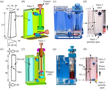
The CFE aboard the ISS included a variety of interior corner flow (ICF) experiment vessels (Bunnel & Weislogel Reference Bunnel and Weislogel2018). A suite of nine low-cost fast-to-flight crew-tended CFE-ICF test vessels representing a variety of container types were constructed for the tests. Wire models of two of the nine vessels flown are provided in figure 5 with critical dimensions identified. The CFE study was conducted over two durations and the results are categorized as CFE-1 and CFE-2. Many of the raw experimental results for CFE-1 are currently openly available for view and download at psi.nasa.gov. Solid models and images for test cells ICF-1 and ICF-4 are also provided in figure 5 for reference.
Wire model, solid model, image and cropped image during double-drain operations on ISS for CFE ICF-1 (a–d) and ICF-4 (e–h), respectively. In addition to a superposition of the relevant coordinate system, (d) and (h) provide bold black arrows indicating piston travel direction and white arrows identifying resulting liquid draining directions with valve 2 fully open and valve 1 partially open to a position where drain flow rates are approximately balanced.

The ICF containers were originally designed to study large length scale passive capillary migration and bubble phase separation, the details of which are described elsewhere (Weislogel et al.
Reference Weislogel, Collicott, Gotti, Bunnell, Kurta and Golliher2004, Reference Weislogel, Jenson, Chen, Collicott, Klatte and Dreyer2007, Reference Weislogel, Chen, Collicott, Bunnell, Green and Bohman2009). Whipper plates (e.g. see figure 5
f,g) designed into the piston reservoirs of ICF units such as ICF-4 were employed in part to deliver bubbly liquids to the test chambers. Remarkably, over 50 approximately 2.5 hour CFE-ICF operations were conducted on a standby basis as astronaut crew time and schedule allowed. For any given operation, the subject ICF vessel is placed on an ISS workbench called the MWA (maintenance work area), backlit by a diffuse light screen via cabin lighting, and filmed via an HD Canon XF305 video camcorder. At the conclusion of each ICF experiment run, the astronaut was instructed to drain most of the liquid from the test section into the reservoir by turning the piston dial. The final drain procedure was always filmed. It was quickly recognized that quantitative analyses of a variety of immediately valuable drain procedures were possible including the present double-drain problem (Weislogel et al.
Reference Weislogel, Baker and Jenson2011). The drain tests are first performed with valve 2 fully open and with valve 1 previously adjusted so that viscous draining resistances through valves 1 and 2 approximately balanced. In this way the primary interior corner of the test cells could be drained at nearly even rates, with adequate symmetry, and while minimizing meniscus elevation at the exit ports without significant gas ingestion (i.e. a double-drain flow; figures 3 and 5). Control of the drain process is maintained by eye and the patient nearly continuous manual rotation of the reservoir piston dial by the astronaut. The double-drain images of figure 5(d,h) are labelled for reference. The time-dependent interface profile provides position
 $h(z,t)$
and volume
 $V(t)$
, which when differentiated with respect to time provides a measure of
 $Q$
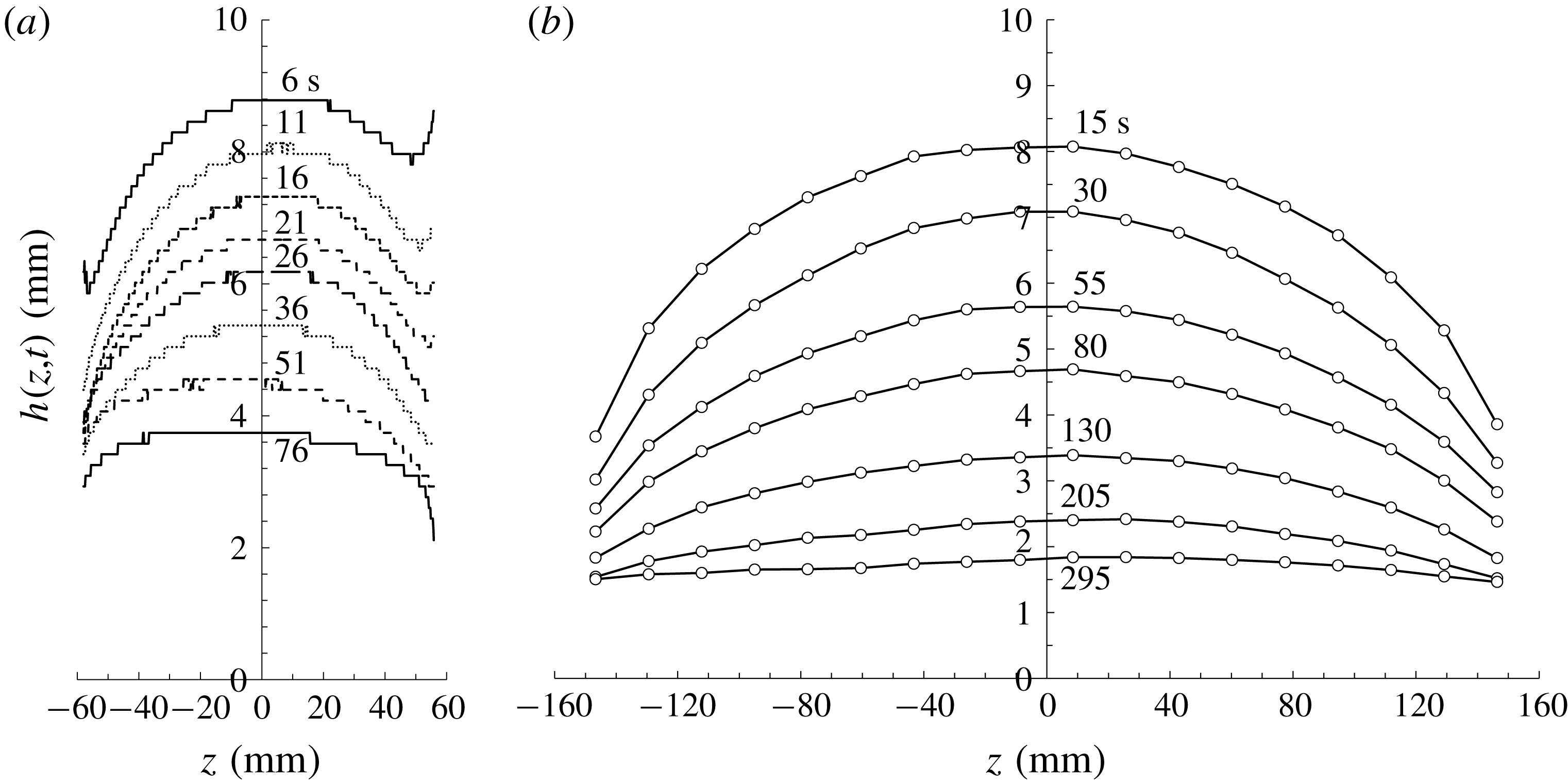
. Sample meniscus centreline profiles at select times are presented in figure 6(a) for an ICF-1 double-drain test. The reduced data from such tests will be discussed shortly.
Double-drain meniscus profiles
 $h(z,t)$
for times listed: (a) space experiment ICF-1 (20 cs PDMS) with drain location at
 $z\approx \pm 63.5$
mm and (b) terrestrial experiment TE-02 (2 cs PDMS) with drain locations at
 $z\approx \pm 157$
mm (see table 1). Experimental uncertainties for
 $h$
are as high as
 $\pm 0.16$
mm in (a), but only
 $\pm 0.028$
mm in (b) (see table 1).

4.2 Terrestrial experiments
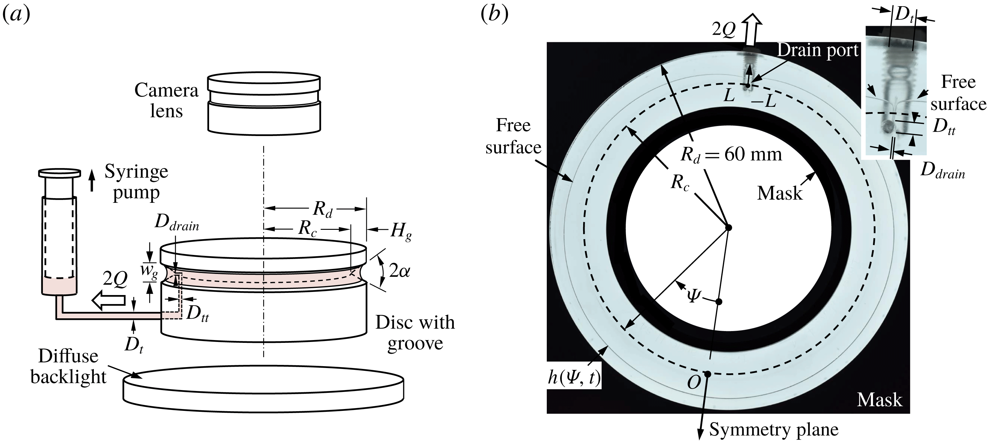
The ICF double-drain tests attempt to achieve symmetry by manual flow control from two exit ports in the manner of figure 3. Improved symmetry is achieved by exploiting a single drain port in the manner of figure 2(c). To this end, terrestrial experiments (TE) are conducted using a circular horizontal flow path and narrow interior corner angle. A schematic of the 120 mm outer diameter clear acrylic test cell fabricated is shown in figure 7 along with critical dimensions and an image of the experiment as viewed from above. The
 $\unicode[STIX]{x1D6FC}=5.62^{\circ }$
interior corner (groove) is lathe cut at low speed using a custom-ground tool. The depth of the groove is
 $H_{g}=10$
mm and the maximum width of the groove is
 $w_{g}=1.97$
mm. The machined surface is progressively sanded using 320 to 3000 grit paper and polished. The groove width is sized to ensure
 $Bo_{g}\equiv \unicode[STIX]{x1D70C}gw_{g}^{2}/\unicode[STIX]{x1D70E}\lesssim 1$
maintaining capillary dominance and increasingly satisfying the model assumptions as the fluid is drained (
 $h\ll H_{g}$
).
The experiments are performed by first filling the groove with liquid and levelling the device via an iterative image analysis approach until a perfect circular meniscus is established;
 $h(\unicode[STIX]{x1D713},t)=\text{const}.$
, where
 $\unicode[STIX]{x1D713}$
is the azimuthal angle (figure 7). The liquid is then removed via a syringe pump adjusted manually to maintain
 $h(L,t)\approx 0$
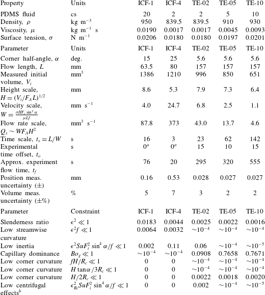
without gas ingestion. The clear acrylic disc is masked to reduce reflections and the process is under-lit by a diffuse light source and filmed from above by a Nikon D750 DSLR camera in time lapse mode. Perfectly wetting polydimethylsiloxane (PDMS) liquids of nominal 2, 5 and 10 cs kinematic viscosities are tested with relevant nominal properties listed in table 1. A simple still image is provided in figure 7(b) for a drain test with 2 cs PDMS (TE-02). The meniscus profile
 $h(\unicode[STIX]{x1D713},t)$
, interior corner vertex at
 $R_{c}=50$
mm, single drain location
 $z=\pm L\approx \pm \unicode[STIX]{x03C0}R_{c}=\pm 157$
mm and symmetry plane location
 $z=0$
are identified in the figure. A magnified image of the drain region is shown in the inset of figure 7(b) where it is observed that the terrestrial experiments achieve
 $h(\pm L,t)\approx 0$
as required by theory, but that the local geometry within the
 $D_{drain}=0.397$
mm inner diameter drain port region does not conform to the analytical requirements of a zero-thickness sink, nor a zero-height sink meniscus.
(a) Terrestrial experiment schematic and (b) sample top view image with key components labelled. The transparent disc is masked to sharpen images collected from the long-working-distance lens. The interior corner vertex
 $R_{c}$
is identified by the dashed line in (b). The drain location detail inset at upper right identifies drain port diameter
 $D_{drain}=0.397$
mm, offset transition tube diameter
 $D_{tt}=1.587$
mm and primary transport tube diameter
 $D_{t}=3.175$
mm, also labelled in (a).

The cylindrical coordinates for
 $h(\unicode[STIX]{x1D713},t)$
are approximated by Cartesian coordinates
 $h(z,t)$
, where
 $z=R_{c}\unicode[STIX]{x1D713}$
with
 $\unicode[STIX]{x1D713}\in [-\unicode[STIX]{x03C0},\unicode[STIX]{x03C0}]$
. Image resolution limitations lead to maximum uncertainties in measured values of
 $h(z,t)$
beginning at
 $\pm 1\,\%$
and ending at
 $\pm 4\,\%$
as
 $h$
decreases with time. Even accounting for centrifugal forces, for our choice of
 $h(z,0)$
and
 $R_{c}$
, the Cartesian coordinate transform introduces maximum errors in
 $V(t)$
of
 ${<}7\,\%$
determined from (2.7) and listed in table 1. These errors decrease to
 ${<}1\,\%$
as draining continues. The experimental flow rate is estimated as
 $Q_{exp}(t)\approx (\unicode[STIX]{x0394}V_{exp}/\unicode[STIX]{x0394}t)|_{t}$
, which produces similarly low errors as time increases. Sample
 $h(z,t)$
data for these terrestrial experiments are shown in figure 6(b) for 2 cs (TE-02). The profiles are notably smoother and more symmetric than those of the ICF-1 test of figure 6(a) due to improved image resolution. We note that due to test cell dimensions the terrestrial tests yield flow rates 2 to 80 times lower than those of the ISS CFE-ICF tests (
 $Q_{s}$
, table 1).
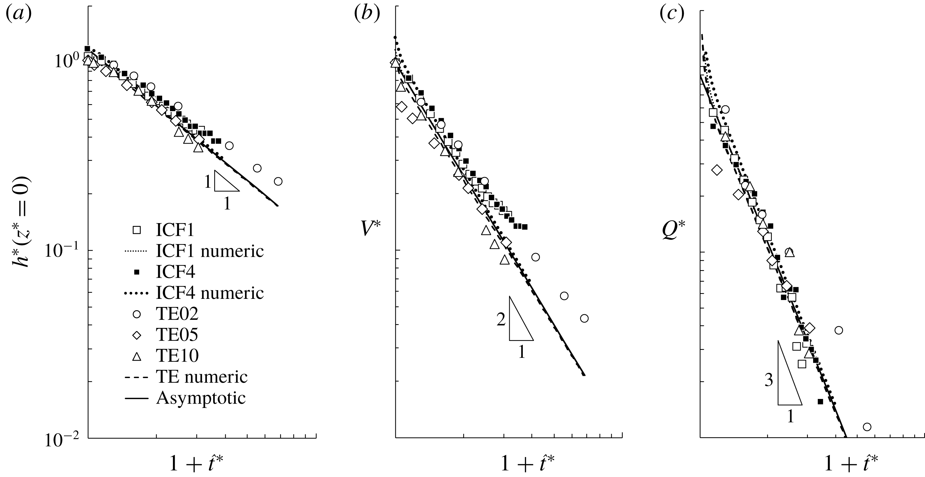
(a) Dimensionless meniscus height at origin (symmetry plane)
 $h^{\ast }(z^{\ast }=0)$
, (b) dimensionless liquid volume
 $V^{\ast }$
and (c) dimensionless flow rate
 $Q^{\ast }$
all in terms of
 $1+\hat{t}^{\ast }$
. We note that the numerical and asymptotic solutions for terrestrial experiments TE-02, TE-05 and TE-10 are nearly coincident. Average uncertainties approximately coincide with symbol size.

Perfectly wetting (
 $\unicode[STIX]{x1D703}=0$
) PDMS test fluid properties, key parameters and constraints of analysis (2.1) and (5.1a–c
). Space experiments are ICF-no and terrestrial experiments are TE-no. We note that
 $h(0,0)$
and
 $H$
are essentially equal.

a Separation of variables profile established before data collection began.
b
 $\unicode[STIX]{x1D716}_{Rc}\equiv H/\unicode[STIX]{x1D713}R_{c}$
, where
 $\unicode[STIX]{x1D713}$
(in radians) is the angle swept out by the liquid column with characteristic wedge radius of curvature
 $R_{c}$
. Inverse viscous resistance function
 $F_{i}\approx 1/7$
in relevant parameters.
5 Data reduction and discussion
At a minimum we seek to confirm the power-law predictions of (2.17), (2.16) and (2.15) where at long times we expect
 $h\sim t^{-1}$
,
 $V\sim t^{-2}$
and
 $Q\sim t^{-3}$
. We first integrate the experimentally determined meniscus profile
 $h(z,t)$
(i.e. figure 6) to find
 $V(t)$
, the discretized time derivative of which yields
 $Q(t)$
. Transforming to dimensionless quantities
 $h^{\ast }$
,
 $V^{\ast }$
and
 $Q^{\ast }$
written as functions of
 $1+\hat{t}^{\ast }$
, we then construct plots such as those shown in figure 8. The results of numerical solutions to (2.8) and the approximate asymptotic analytic solution of (3.6) are overlaid on the figure for comparison. The numeric and asymptotic analytical predictions converge at long times and agree favourably with the data trends and the scaled power-law slopes sketched in the figure. Respective maximum average experimental uncertainties for
 $h^{\ast }$
,
 $V^{\ast }$
and
 $Q^{\ast }$
are
 $\pm 4\,\%$
,
 $\pm 7\,\%$
and
 $\pm 4\,\%$
for worst case ICF-4 with average errors represented by the size of the symbols employed in figure 8. Uncertainties are highest for the volume measurements and increase with time up to
 $\pm 12\,\%$
for ICF-4. We note that
 $h^{\ast }\approx 1.178/(1+\hat{t}^{\ast })$
from (2.17),
 $V^{\ast }\approx 1/(1+\hat{t}^{\ast })^{2}$
from (2.16) and
 $Q^{\ast }\approx 0.907/(1+\hat{t}^{\ast })^{3}$
from (2.15), which are appropriate for all test cases. The numerical prediction for
 $h^{\ast }(z^{\ast }=0)$
for the case of ICF-4 in figure 8(a) is essentially coincident with both the TE numeric and asymptotic predictions. It is also noted that the numerical solutions for
 $h^{\ast }$
,
 $V^{\ast }$
and
 $Q^{\ast }$
for the terrestrial experiments TE-02, TE-05 and TE-10 are also essentially coincident.
In terms of dimensional quantities
 $1+\hat{t}^{\ast }=1+W(t-t_{o})/t_{i}^{\ast }L$
. For arbitrary drain initiation time less than
 $t_{o}$
, the dimensional, experimentally determined time
 $t_{o}$
required for the meniscus profile to first achieve the separation of variables profile establishes the appropriate initial conditions with which to compare the experiments with theory, namely
 $h(0,t_{o})$
and
 $V(t_{o})\equiv V_{i}$
. Experimentally determined values for
 $t_{o}$
are listed in table 1 for the experiments conducted. For the terrestrial tests, the separation of variables profile is rapidly achieved as evidenced by the low ‘best fit’ empirically determined values for
 $t_{o}$
as compared to the total experiment flow time
 $t_{f}$
also listed in table 1. In general, the separation of variables form is achieved well within 8 % of the total flow times recorded. (We note that the conditions for low inertia and low centrifugal effects are identical for the terrestrial experiments in table 1.) For the ICF experiments, the separation of variables profiles were already established prior to the data collection procedure and
 $t_{o}\approx 0$
is appropriate for these tests.
The parameters of the terrestrial and space experiments may be used to assess the degree to which the manifold assumptions of the theory are satisfied. For example, to neglect both corner curvature effects on the area functions and to achieve an essentially Cartesian flow one must respectively satisfy
 $$\begin{eqnarray}\frac{fH}{R_{c}}\ll 1,\quad \frac{H\tan \unicode[STIX]{x1D6FC}}{3R_{c}}\ll 1,\quad \frac{H}{2R_{c}}\ll 1.\end{eqnarray}$$
These parameters along with others are defined and characteristic values calculated and listed in table 1. All constraints are increasingly satisfied as time increases. However, non-negligible inertia may be present at the initiation of space experiments ICF-4, where values for
 $\unicode[STIX]{x1D716}^{2}SuF_{i}^{2}\sin ^{4}\unicode[STIX]{x1D6FC}/f$
are up to two orders of magnitude larger than for the terrestrial tests conducted.
6 Conclusions with implications for design
Barring such complicating impacts of fluid contamination, finite surface roughness and heterogeneity, van der Waals forces, body forces such as gravity and others, under the constraints primarily of a slender interior corner wetting capillary flow, the symmetric corner draining solutions of this work for perfectly wetting liquids anticipate power-law relationships for characteristic meniscus height
 $h\sim t^{-1}$
, liquid volume
 $V\sim t^{-2}$
and maximum drain rate
 $Q\sim t^{-3}$
. At long times, these relationships are confirmed by low-gravity and terrestrial experiments, equations (2.17), (2.16) and (2.15), respectively.
The analytical results are maximal due to an idealized sink condition where the meniscus is drawn down to a zero height at the liquid drain location(s),
 $h(\pm L,t)=0$
. The results may be used to quickly estimate the limiting drain rates possible under such constraints. Numerical solutions are provided to confirm the asymptotic analytical results which become increasingly accurate in time as the flow becomes increasingly slender. Simple relationships as functions of the fluid properties and corner dimensions are available for the time required to drain an amount of liquid, which may be useful to predict fuel recovery from spacecraft tanks where both time and liquid volume are high-value commodities.
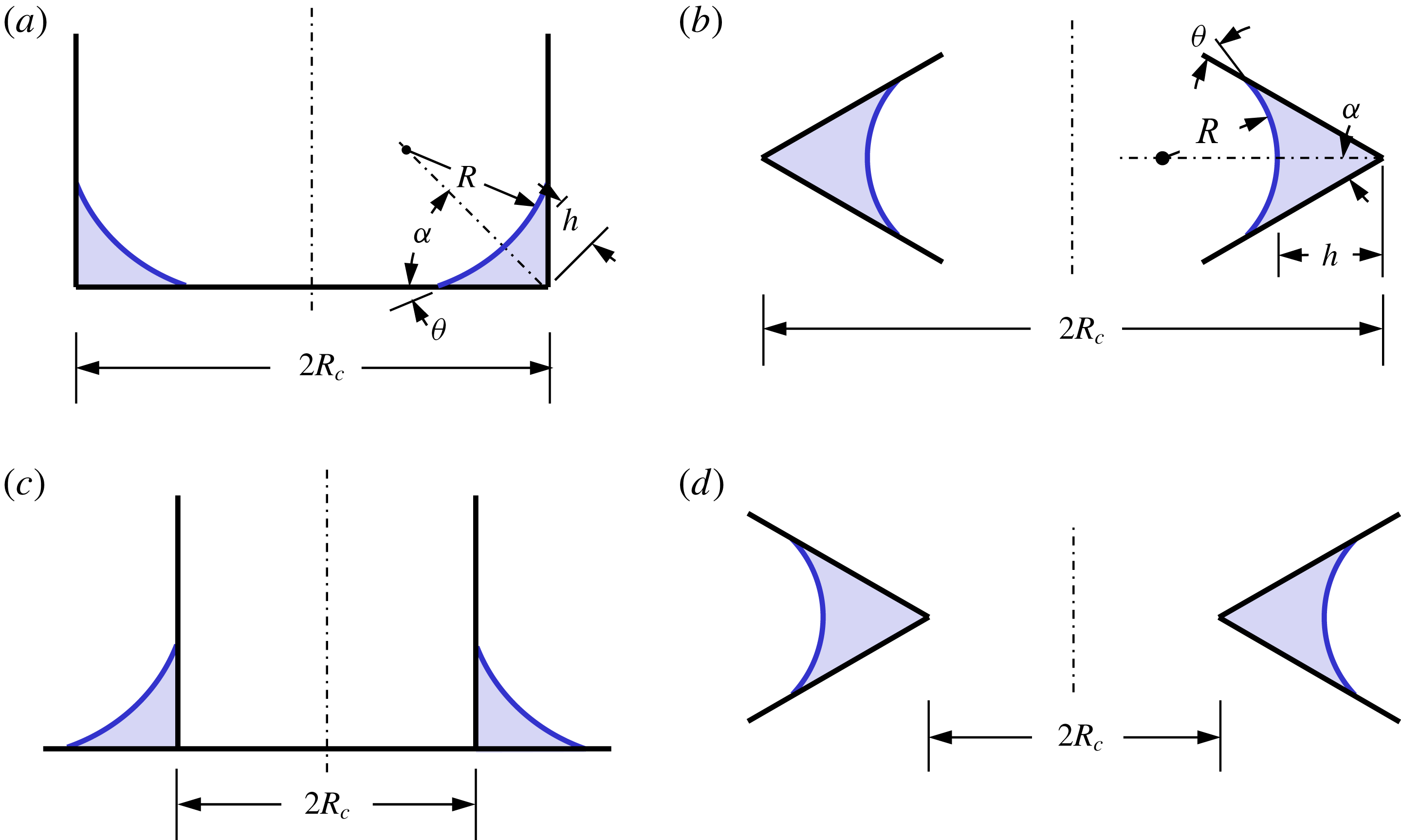
(a–d) Applicable rotationally symmetric interior and exterior corner draining geometries, where
 $L=\unicode[STIX]{x03C0}R_{c}$
and
 $Q_{tot}=2Q$
. Arbitrary closed interior corner circuits may also be analysed in a like manner provided a local corner curvature can be characterized by
 $1/R_{c}$
satisfying the additional model constraints of predominately one-dimensional flow, namely
 $fH/R_{c}\ll 1$
,
 $H\tan \unicode[STIX]{x1D6FC}/3R_{c}\ll 1$
,
 $H/R_{c}\ll 1$
and
 $\unicode[STIX]{x1D716}_{Rc}^{2}SuF_{i}^{2}\sin ^{4}\unicode[STIX]{x1D6FC}/f\ll 1$
.

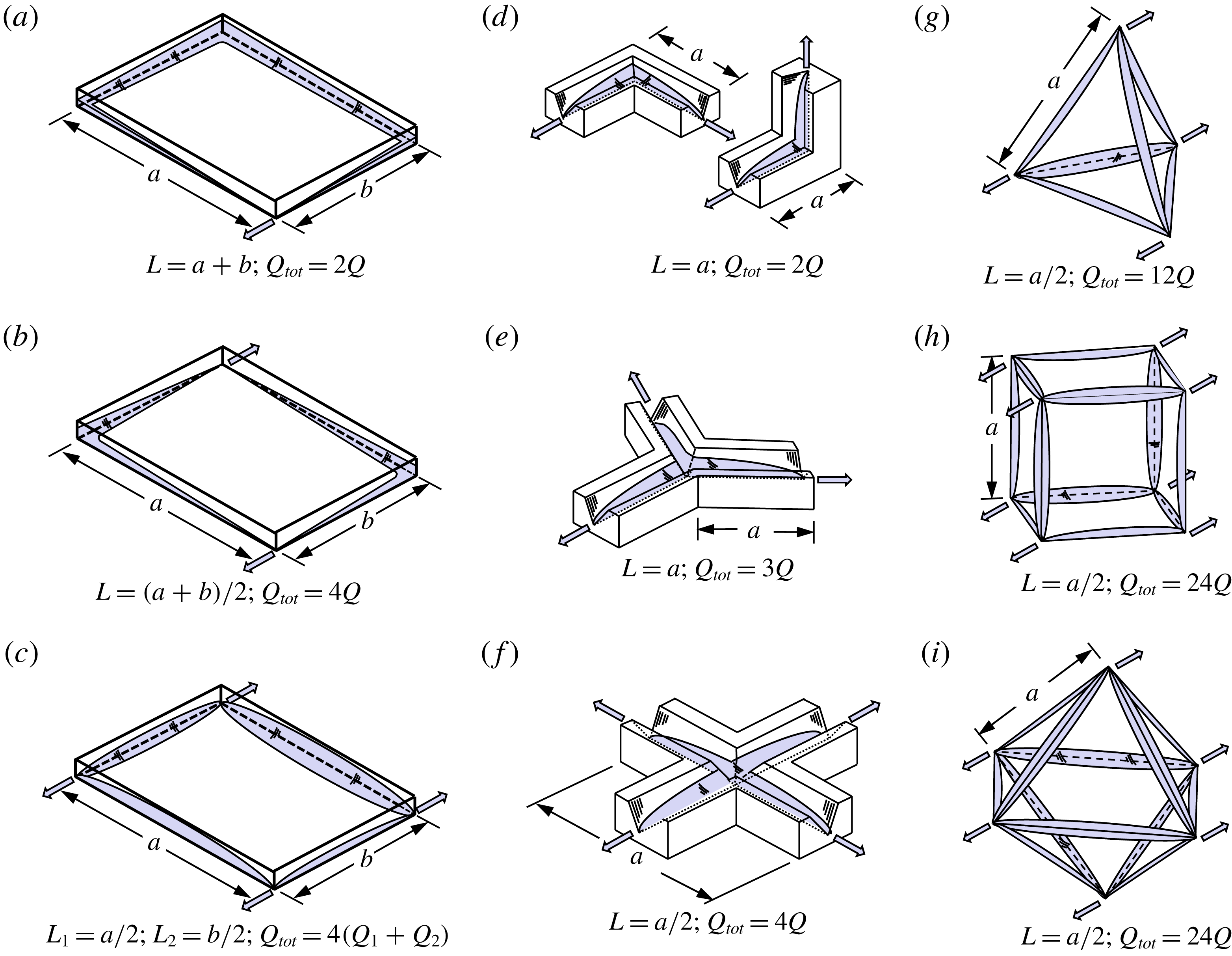
Further samples of applicable drain scenarios modelled by the present theoretical approach: (a–c) open shallow rectangular trays, (d–f) open interior corner networks and (g–i) enclosed regular polyhedrons. Large arrows denote drain locations. Flow lengths
 $L$
and total flow rates
 $Q_{tot}$
are noted as functions of characteristic container dimensions.

The self-limiting capillary draining flow scenario is most directly described mathematically as a symmetric double-drain problem as depicted in figure 3. However, for slender flows, certain single-drain location flows are applicable as presented in figure 2 and as demonstrated experimentally in figures 6(b) and 7. In figure 9 are sketched several additional rotationally symmetric geometries readily addressed by the present analytical approach. In such cases, if the corner radius is represented by
 $R_{c}$
, the flow length is
 $L=\unicode[STIX]{x03C0}R_{c}$
and
 $Q_{tot}=2Q$
with all solutions and constraints of this work applicable. The analysis may also be applied to model capillary draining phenomena from interior corner networks, as sketched in figure 10 for a representative selection of shallow trays, triangular groove networks and regular polyhedrons. The analysis succeeds provided the impact of three-dimensional free surface curvature in the interior corner junction regions is small, which is increasingly likely as time increases during drain. For each example in figure 10, the flow length
 $L$
for the particular drain scenario is provided together with the total drain flow rate
 $Q_{tot}$
, consistent with the notation of the present analysis. We note in general that
 $Q_{tot}\sim 2nm/L$
, where
 $n$
is the number of corners drained at
 $m$
sink locations.
Acknowledgements
This work was conducted under National Aeronautics and Space Administration cooperative agreement NNX09AP66A. Special thanks are due to NASA astronauts M. Hopkins, S. Swanson and S. Kimbrough, JAXA astronaut K. Wakata and ESA astronaut A. Gerst, who together completed the capillary flow experiments for the CFE-2 ICF-1 and ICF-4 vessels on the ISS. Their creativity and patience during flight operations led to numerous peripheral observations of which the subject of this paper is but one. Special thanks are also due to J. Geile and A. Wollman for assistance with data reduction and to the NASA cadre at Glenn Research Center, Johnson Space Center and Marshall Spaceflight Center. B. Semerjian fabricated the terrestrial test cell.