1. Introduction
In this paper, we examine the general equilibrium implications of climate change for Ethiopia, a low-income country in East Africa. There is a risk that climate change will have devastating effects on Ethiopian agriculture. Given that a large share of the country's population depends on agriculture, this may have huge impacts on the entire economy. We therefore examine the economic impacts of climate change-induced adjustments, using a countrywide computable general equilibrium (CGE) model.
Understanding the potential economy-wide impacts of climate change for a given country is critical both in designing national adaptation strategies as well as in formulating effective global climate policy agreements. A developing country needs adaptation policies that are tailored to the anticipated impacts for that specific country. Quantifying the impact of climate change on the overall economy can, therefore, provide an important guide to policy.
Agriculture, especially rain-fed agriculture, is likely to be substantially affected by climate change (Sachs et al., Reference Sachs, Panatayou and Peterson1999; Antle, Reference Antle2010). Hence, countries with large agricultural sectors in the tropics and subtropics where agricultural production is weather sensitive and adaptive capacities are low are likely to bear the brunt of the adverse economic impacts of climate change. Numerous partial equilibrium studies assess the micro-level impacts of climate change on agricultural performance in developing countries (see, for example, Rosenzweig and Parry, Reference Rosenzweig and Parry1994; Reilly et al., Reference Reilly, Baethgen, Chege, Watson, Zinyowera, Moss and Dokken1996; Reilly and Schimmelpfennig, Reference Reilly and Schimmelpfennig1999; Kates, Reference Kates2000; Kurukulasuriya and Mendelsohn, Reference Kurukulasuriya and Mendelsohn2006; Deressa, Reference Deressa2007; Seo and Mendelsohn, Reference Seo and Mendelsohn2008a, Seo and Mendelsohn, Reference Seo and Mendelsohn2008b; Deressa and Hassan, Reference Deressa and Hassan2009; Seo et al., Reference Seo, Mendelsohn, Dinar, Hassan and Kurukulasuriya2009).
Given the importance of agriculture for economic activity, employment and livelihood in many developing countries, a loss of agricultural productivity caused by climate change is likely to affect the entire economy of these countries. Many other sectors of the economy, not only those concerned with processing and distributing agricultural products, are likely to experience indirect effects through impacts on income and consumption. In sum, because climate change may affect various sectors of the economy directly or indirectly, interactions between different sectors need to be studied to assess the impacts of climate change on agriculture. CGE models are well suited to depict interactions between agriculture and other sectors of the economy.
How countries cope with shocks to agriculture will depend not only on the magnitude of the initial shock. Previous experience indicates that economies subject to significant external shocks have been shown to respond differently. For example, Balassa (Reference Balassa1985) studied the impact of the oil crisis in the 1970s on developing countries, and found significant differences among countries in terms of the crisis's impacts on economic growth, suggesting that the countries in question differed in terms of their responsiveness to such shocks. These differences can be attributed to the explicit adjustment policies applied, but also to differences in trade policy and trade patterns, the rate of growth of the labour force, and investment rates, as well as (of course) the initial level and structure of economic activity. It seems likely that climate change will also affect countries differently, not only because of differences in the explicit adjustment or adaptation policies implemented, but also because of a wide range of other factors.
The objective of this paper is to make a general equilibrium analysis of the potential impacts of climate change. We simulate the future development of the Ethiopian economy over a 50-year period using results from a Ricardian model (discussed in more detail below) and based on two different scenarios for total factor productivity (TFP) growth: one with no growth at all during the projected period, and one with the average growth for the period of political and economic reforms which started in 1992, each of which develop with and without the climate change situation. That is, we directly compare growth within a scenario with and without climate change. We incorporated climate change into the model by letting land and livestock productivity decline over time, and compared the outcomes for a 50-year period.
Climate change has recently attracted the attention of various stakeholders in Ethiopia. A national climate change forum and a civil society network on climate change have been established, for example, and the country has submitted its National Adaptation Programme of Action (NAPA) and Nationally Appropriate Mitigation Action (NAMA) plans in respect of climate change to the United Nations Framework Convention on Climate Change (UNFCCC). Impacts of current climate variability identified in the NAPA document include: food insecurity due to drought and flood events; outbreak of sicknesses such as malaria, water-borne diseases and respiratory diseases; and land degradation due to heavy rainfall.
The following conclusions can be drawn from the Ethiopian studies reviewed. First, there are very few studies that look into the impacts of climate change in Ethiopia in general and its economy-wide impact in particular. Secondly, most of the studies were concerned with the microeconomics of climate change (Deressa et al., Reference Deressa, Hassan, Alemu, Yesuf and Ringler2008a, Reference Deressa, Hassan and Ringler2008b). However, climate change might be expected to have area-specific effects – often of interest on the scale beyond the household/micro level. For example, agro-ecology based analyses applying a CGE model might provide better or at least additional insights into the impact of climate change. Thirdly, and more importantly, even though mixed crop/livestock farming dominates Ethiopian agriculture, climate change studies (cf. Deressa, Reference Deressa2007; Yesuf et al., Reference Yesuf, DiFalco, Ringler and Köhlin2008; Deressa and Hassan, Reference Deressa and Hassan2009) have all focused on crop agriculture and disregarded the role of livestock. There appear to be significant linkages (and tradeoffs) between the crop and livestock subsystems within the farm household system, particularly at times of stress, which is another dimension of interest in climate change studies. Intuitively, however, climate change would also be expected to affect livestock production differently (Kurukulasuriya et al., Reference Kurukulasuriya, Mendelsohn and Hassan2006; Seo and Mendelsohn, Reference Seo and Mendelsohn2008a, Reference Seo and Mendelsohn2008b). Hence, omitting livestock production could misestimate the impact of climate change. Therefore, it is of interest to look at the economy-wide impact of climate change inclusive of livestock production. Arndt et al. (Reference Arndt, Robinson and Willenbockel2011) and Robinson et al. (Reference Robinson, Willenbockel and Strzepek2012, Reference Robinson, Strzepek and Cervigni2013) did look at the impacts on poverty and welfare, but focused on the shorter term impacts of climate variability only, rather than the impacts of longer term changes in average climate.
The key contributions of this study are that it analyzes the economy-wide effects, i.e., to other sectors of the economy, of the impact of climate change on agriculture in Ethiopia inclusive of livestock. The fact that it uses the results of a Ricardian model that takes into account efficient autonomous adaptation by farmers as an input in the simulation also makes it different from the Development Prospects Group study. We also consider a longer time horizon, i.e., we simulate the impact of climate change over 50-year periods into the future which is of relevance in policy respects as opposed to the shorter time horizon (i.e., 25 years) considered in the Development Prospects Group (2008) study. The agro-ecology dimension considered in our study is an additional contribution.
The rest of the paper is organized as follows: in section 2, we review climate change and CGE models. Section 3 highlights climate characteristics and the Ethiopian economy, as well as the potential impacts of climate change on agriculture. Section 4 outlines the CGE model used in this analysis, and shows how climate change is included in the model. Section 5 presents a discussion of the study results, while section 6 concludes the paper.
2. Climate change and CGE models: literature review
There has been an explosive growth in analyses of developing countries' vulnerability to climate change, and there are by now a number of studies that look into the economy-wide impacts of climate change in the context of developing countries in fashions similar to ours. Reid et al., (Reference Reid, Sahlén, Stage and MacGregor2008), for example, use a CGE model to estimate the impacts of changed agricultural productivity and changed fish availability on the Namibian economy. They use a static analysis, where little or no adaptation or economic change was assumed to take place.
Another study, by Thurlow et al., (Reference Thurlow, Zhu and Diao2009), assesses the impact of climate variability and change on economic growth and poverty in Zambia. The investigation combines a hydro-crop model with a dynamic CGE model as an analytical tool. Their findings reveal that climate variability has cost the country US$4.3bn over a 10-year period. Thurlow et al. (Reference Thurlow, Zhu and Diao2009) also find that these losses would reach as high as US$7.1bn under a worst-case rainfall scenario, and that most of the negative impacts of climate variability are concentrated in the southern and central regions of the country, where food insecurity is most vulnerable to climate shocks. On the whole, they find that, by 2016, climate variability would keep 300,000 people below the national poverty line.
A study by Arndt et al. (Reference Arndt, Strzepeck, Tarp, Thurlow, Fant and Wright2010) focuses on the potential impacts of climate change on Mozambique. They employ a framework of integrated modelling that translates outcomes of general circulation models (GCMs) to atmospheric changes that are, in turn, projected into biophysical outcomes with the help of hydrological, crop, hydropower and infrastructure models. The sector models allow simulations that compared a historical baseline with four different climate change scenarios that were used to estimate economy-wide impacts in terms of damage costs and national welfare losses through a dynamic CGE model. The study identifies adaptation measures such as improved road design, agricultural sector investments, cooperative river basin management and the regional coordination of adaptation strategies.
Bezabih et al. (Reference Bezabih, Chambwera and Stage2011) analyze the economic impacts of climate change-induced adjustments on the performance of the Tanzanian economy, using a countrywide CGE model. In this study, the effect of overall climate change on agricultural productivity is projected to be relatively limited to begin with, but will then become progressively worse. However, the long time periods involved and the low starting point of the economy leave ample time for factor substitutability, which will allow adaptation measures to replace reduced land productivity with increased use of capital and labour. Therefore, the authors find that the overall impact on the Tanzanian economy might be quite limited in the longer term.
Zhai et al. (Reference Zhai, Lin and Byambdorj2009) examine the potential long-term impacts of global climate change on agricultural production and trade in the People's Republic of China (PRC), using an economy-wide, global CGE model, as well as simulation scenarios of global agricultural productivity change induced by climate change up to 2080. The study suggests that, with a declining share of agriculture in the gross domestic product (GDP), the impact of climate change on the overall macroeconomy is moderate. Food processing sectors carry the burden of some crop sectors (wheat in particular) that are likely to expand due to increased demand.
The Development Prospects Group (2008) examines the economic im-pacts of climate change on Ethiopia. They use the 2005/2006 Social Accounting Matrix (SAM) for Ethiopia constructed by the Economic Development Research Institute (EDRI) and the Institute of Development Studies (IDS). The impacts of climate change – taken as changes in mean temperatures and rainfall – on agricultural productivity are obtained from estimates made with a Ricardian model. The study reports the outcomes of five simulation runs of the model in addition to the baseline run made in the absence of climate-related shocks. The first simulation is the reproduction of Ethiopia's historical stochastic experience. Key findings of the study include that, in the worst-case scenario, real GDP in the final year (in a period of 25 years) would be 46 per cent lower than in the baseline run. The burden of adjustment appears to fall more on consumers, since aggregate consumption – which is dependent on agriculture – exhibits more variation. The variation of aggregate absorption is lower than that of GDP, indicating that international trade serves to dampen the impact of climate change.
Although this is a comparative-static analysis, Mideksa (Reference Mideksa2010) looks at the impact of climate change on Ethiopia's economy and tries to examine its distributional consequence using the Gini-coefficient. Arndt et al. (Reference Arndt, Robinson and Willenbockel2011) and Robinson et al. (Reference Robinson, Willenbockel and Strzepek2012, Reference Robinson, Strzepek and Cervigni2013) also look at climate change in Ethiopia. Arndt et al. (Reference Arndt, Robinson and Willenbockel2011) develop a stochastic economy-wide framework where emphasis is given to the development of a prior subjective distribution of future climate outcomes. Their results suggest the importance of cumulative processes and rates of growth. Their results also imply that poor consumers are those who are likely to experience increased vulnerability. Robinson et al. (Reference Robinson, Willenbockel and Strzepek2012) employ a CGE model of Ethiopia encompassing a system of country-specific hydrology, crop, road and hydropower engineering models to simulate the economic impacts of climate change scenarios from GCMs to 2050. They find that Ethiopia's GDP in 2050 will be up to 10 per cent below compared to the baseline counterfactual of no climate change (historical climate) especially in the absence of policy-driven adaptation investments that are either externally or domestically funded. They also argue that suitably designed adaptation investments could restore aggregate welfare to baseline levels at a cost substantially lower than the welfare losses as a result of climate change.
Non-economic impacts, such as health impacts, following responses made to climate change have also served as subjects of CGE analyses. For example, Pattanayak et al. (Reference Pattanayak, Ross, Depro, Bauch, Wendland and Alger2009) examine the general equilibrium outcomes of a Brazilian policy to expand forests by 50 million ha. Their results indicate that there would be a small decline in GDP, some decline in the welfare of urban households, and fewer opportunities for subsistence agriculture for rural households, but net welfare would improve due to the health benefits derived from the conservation of nearby forests.
3. Climate characteristics and the Ethiopian economy: a background
Ethiopia is heavily dependent on rain-fed agriculture. Its geographical location and topography, in combination with a low adaptive capacity, make the country highly vulnerable to the adverse impacts of climate change. With a population of more than 72 million, poverty in Ethiopia is a chronic problem, with about two-thirds of the population living on less than US$2 a day (World Bank, Reference Bank2008). The country is one of the most food insecure in the world, as manifested by protracted hunger and famine. About 74 per cent of the population of the country derive their livelihood from agriculture. Of the 4.3 million ha of potentially irrigable agricultural land, less than 10 per cent is currently farmed. Smallholder farmers dominate the sector, generating about 90 per cent of agricultural output (Adenew, Reference Adenew2006; MoARD, 2010).
Economic performance was dismal during most of the second half of the 20th century. Between 1950 and 1990, Ethiopia's TFP actually declined by over 1 per cent per year. In the post-1992 reform period, on the other hand, its economic growth was among the highest in Africa, with TFP growth registering over 2.5 per cent per year. Important constraints remain, however, in the forms of insecure property rights to land and an as yet poorly developed private sector (Easterly, Reference Easterly2006).
Geographically, Ethiopia can be subdivided into five agro-ecological zones based on the diversity of moisture and on land use. There are drought-prone highlands where rainfall is insufficient, rainfall-sufficient highlands where enset-based farming systems dominate, and rainfall-sufficient highland areas where cereal-based farming systems dominate. The lowland areas bordering on Eritrea are generally dry and are dominated by pastoralism, while the lowland areas further inland are humid and are currently dominated by crop farming. Climate change can be expected to lead to shifts in suitable cultivation patterns in all five regions described above. Whether middleman markets for inputs and outputs can change in time to let farmers cope with these shifts will be an important challenge for future adaptation policy.
Ethiopia has experienced at least five major national droughts since 1980, along with large numbers of localized ones (World Bank, Reference Bank2008). These cycles of drought create poverty traps for many households, constantly dwarfing efforts to build up assets and increase income. Evidence shows that about half of all rural households in the country experienced at least one major drought during the five years preceding 2004 (Dercon, Reference Dercon2009). With agriculture highly dependent on rainfall, rain and – more generally – weather rule the lives and wellbeing of many rural people in Ethiopia. The weather determines whether they will have enough to eat, be able to provide basic necessities, and earn a living. Indeed, farmers' dependence on rainfall and its erratic patterns has largely contributed to the food shortages and crises with which they constantly battle.
Ethiopia, like many other African countries, has a range of factors that may undermine communities' ability to adapt to climate change (Boko et al., Reference Boko, Niang, Nyong, Vogel, Githeko, Medany, Osman-Elasha, Tabo, Yanda, Parry, Canziani, Palutikof, Van der Linden and Hanson2007). The country has a complex climate system and combines this with socio-economic challenges such as endemic poverty, limited access to capital and global markets, ecosystem degradation, complex disasters, and conflicts. Accordingly, the effect of climate change on the performance of Ethiopia's economy is likely to be a function of both the structure of the macroeconomy and sector-specific vulnerability. This means that the government's adaptation policies are likely to be crucially important. However, such policies are apt to be costly and, without a realistic baseline scenario, there is a risk that government programmes will be evaluated against an inappropriate no-cost, no-climate-change status quo rather than against the outcomes that will prevail if no government adaptation is carried out (Stage, Reference Stage2010). It is important, therefore, to assess what impacts climate change is likely to have if private agents are left to adapt on their own. Such a baseline impact assessment can be used to evaluate the effects of activist adaptation policies.
4. Modelling impacts on the Ethiopian economy using a CGE model
4.1. The CGE model framework
In the last three decades, CGE models have been widely used for policy analysis, particularly to evaluate the economy-wide and distributional welfare effects of economic changes, in both developed and developing countries. More recently, CGE models have been applied to analyzing the impacts of climate change.
CGE models consist of numerical models of all supply-and-demand relationships in an economy. The model baseline is then calibrated using current economic data, usually from a SAM, and the model can then be used to simulate the effects of external shocks, changes in economic policy, or changes in economic structure. Using CGE analysis is appropriate as the impacts of climate change are generally economy wide in nature, and would lead to strong general equilibrium feedback effects. Moreover, production-related shocks emanating from climate change might also lead to differential effects or welfare consequences being experienced by different social groups or households.
In our study, we simulated the impacts of climate change-induced variations in respect of land productivity on the Ethiopian economy in the 2010–2060 period. We used a dynamic CGE model with a SAM that has a detailed depiction of production by sector, including agriculture and manufacturing. The basic CGE framework follows the generic International Food Policy Research Institute (IFPRI) model closely (see Löfgren et al., Reference Löfgren, Harris, Robinson, Thomas and El-Said2002, for a detailed discussion). The standard IFPRI CGE model explains all payments recorded in the SAM. The model essentially follows the SAM disaggregation of factors, activities, commodities and institutions. The model is specified as a set of simultaneous equations, most of which are non-linear, and there is no objective function. The equations define the behaviour of the different actors. For production and consumption decisions, behaviour is captured by non-linear, first-order optimality conditions. That is, production and consumption decisions are driven by the maximization of profits and utility, respectively. The equations also include a set of constraints such as market equilibria (for factors and commodities) and macroeconomic aggregates (balances for savings-investment, the government, and the current account with the rest of the world) that have to be satisfied by the system as a whole, but are not necessarily considered by any individual actor.
Each producer (represented by an activity) is assumed to maximize profits, defined as the difference between revenue earned and the cost of factors and intermediate inputs. Profits are maximized subject to a production technology. The technology is specified by a constant elasticity of substitution (CES) function of the quantities of value added and a Leontief function of aggregate intermediate input. Each activity produces one or more commodities according to fixed-yield coefficients. In addition, a commodity may be produced by more than one activity. The revenue of an activity is defined by the level of the activity, yields, and commodity prices at the producer level. As part of its profit-maximizing decision, each activity uses a set of factors up to the point where the marginal revenue product of each factor is equal to its wage (also called factor price or rent). Factor market closures equilibrate supplies and demands in each factor market, with the quantity supplied of each factor fixed at the observed level. An economy-wide wage variable is free to vary to ensure that the sum of labour demands from all activities equals the quantity of labour supplied. Each activity pays an activity-specific wage; this is a product of, on the one hand, the economy-wide wage and, on the other hand, a fixed, activity-specific wage distortion term.
In the CGE model, institutions are represented by Households, Enterprises, Government, and the Rest of the world. Households – disaggregated as in the SAM – receive income (directly or indirectly, via Enterprises) from the factors of production as well as transfers from other institutions. Transfers from Rest of the world to Households are fixed in foreign currency. The same holds true for all transfers between Rest of the world and domestic institutions (Households and Enterprises) and factors. Households use their income to pay direct taxes, save, consume and make transfers to other institutions. The direct taxes and transfers to other domestic institutions (Enterprises, Government and other Households) are regarded as fixed shares of Household income, whereas the savings share is flexible for selected Households. Household consumption covers marketed commodities, purchased at market prices that include commodity taxes and transaction costs, and home commodities, which are valued at activity-specific producer prices. Household consumption is allocated across different commodities (both market and home commodities) according to linear expenditure system demand functions, derived from the maximization of a Stone–Geary utility function.
Enterprises may also receive transfers from other institutions. Enterprise incomes are allocated to direct taxes, savings, and transfers to other institutions. Enterprises do not consume.
Government collects taxes at ad valorem rates and receives transfers from other institutions. Government uses this income to purchase commodities for its consumption and for transfers to other institutions. Government consumption is fixed in real (quantity) terms whereas Government transfers to domestic institutions (households and enterprises) are indexed to the Consumer Price Index. Government savings, i.e., the difference between Government income and spending, is assumed to be fixed and tax rates are assumed to be adjusted each year in order to maintain a fixed level of government savings.
The final institution is Rest of the world. The rest of the world purchases Ethiopian exports (the optimal mix between production for the domestic market and production for the export market is determined for each commodity traded in both markets using a CET (constant elasticity of transformation) function) and provides Ethiopia with import goods (for commodities that are both produced domestically and imported, the optimal mix is determined using a CES function). Transfer payments between Rest of the world and domestic institutions and factors are all fixed in foreign currency. Foreign savings or the current account deficit is the difference between foreign currency spending and receipts. The current account is assumed to be fixed in real terms and the real exchange rate is assumed to adjust accordingly.
In our formulation, the static CGE model is expanded into a dynamic CGE model for 2010–2060 using a recursive framework. This means that the model is solved for an individual year; savings and investment rates are used to update the capital stocks in various sectors, and the new values for the capital stocks are used in the solution for the subsequent year. In addition to this, numerous other values such as the size of the population and of the labour force are updated from one year to the next.
4.2. Scenario considerations
In the scenario development we employed the Ricardian model, as discussed above, to incorporate the impact of climate change in a CGE. We draw on the Ricardian results from Gebreegziabher et al. (Reference Gebreegziabher, Mekonnen, Deribe, Abera and Kassahun2013) to model the impacts on agriculture of the changes in temperature and precipitation due to climate change as indicated by the climate projections from the IPCC's A1B scenario which in turn is used for modelling the economy-wide effects. Accordingly, climate change impact is assessed using a Ricardian model for the Nile basin of Ethiopia. The data set we used for the study comes from a survey of 1,000 cross-sectional farm households in the Nile Basin of Ethiopia. The survey was carried out during the 2004/2005 production year and covered five regional states of Ethiopia and 20 districts. The sample districts were purposely selected to include different attributes of the basin such as: agro-ecological zones; the degree of irrigation activity (percentage of cultivated land under irrigation); average annual rainfall; rainfall variability (coefficient of variation for annual rainfall); and vulnerability. One peasant association was selected from each district, making a total of 20, by the purposive sampling method to include households that irrigate their farms. Once the peasant associations were chosen, 50 farmers were selected at random from each peasant association, making the total sample size 1,000 farmers.Footnote 1
The Ricardian model is specified using net revenue obtained separately from crop and livestock. Net revenue from crop production is defined as gross crop revenue less the total associated cost of production calculated for each agricultural household; net revenue from livestock is defined in an analogous fashion. Then, these net revenues are used as dependent variables (and regressed separately) specified as functions of the following set of regressors: (i) climate variables (temperature and precipitation); (ii) soil types/characteristics; and (iii) socio-economic variables like household characteristics (and characteristics of farm firm), institutional support and infrastructure. That is, Ricardian models are estimated with net crop revenue and net livestock revenue as dependent variables and with climate variables entering as linear, squared and crossed (interaction) terms between precipitation and temperature. Most of the interaction terms and squared terms included in the estimation turned out to be significant in addition to the linear terms implying that climate has a nonlinear effect. The Ricardian model results relating to climate variables are provided in tables A1, A2 and A3 in the online Appendix available at http://journals.cambridge.org/EDE. Marginal effects of climate variables are calculated based on coefficient estimates. The marginal impact analysis finds that a 1°C increase in annual temperature will lead to an average change in net revenue of −1,577.72 Ethiopian Birr (ETB) from crop agriculture and 282.09 ETB from livestock, but with the impacts differing for different parts of the country depending on the initial annual temperature. These changes are statistically significant at the 1 and 5 per cent levels, respectively. A 1 mm/month increase in annual precipitation will have significant positive effects on average net crop revenues and net farm revenue (ETB 183.19) but negative average impact on net livestock revenue, −163.78 ETB; again, while this is the average impact, impacts will differ across the country depending on the initial levels of rainfall. Moreover, the study also analyzed the impact of forecasted uniform climate scenarios and impacts of specific climate change scenarios predicted by AOGCMs (Atmospheric-Oceanic Global Circulation Models). Specifically, we used the scenario predictions from CGCM2, HadCM3, and PCM following Strzepek and McCluskey (Reference Strzepek and McCluskey2007) and Deressa and Hassan (Reference Deressa and Hassan2009). Details are provided in table A4 in the online Appendix. These climate scenarios were used to estimate the local effects of climate change on net revenue for the different agro-ecological zones of Ethiopia. The effect of climate on net revenue for different agro-ecological zones is calculated as percentage change originally (see table A5 in the online Appendix). Therefore, we impute the change in net revenue as a percentage when shocking the productivity of land or livestock. We let productivity decline to near zero but not to zero or beyond, so never more than -100 per cent compared to the baseline despite what is reported in the table.
The impact of climate change is modelled as declining productivity in the land and livestock assets, rather than as declining agricultural yields, using the Ricardian impact estimates for each agro-ecological zone. This provides scope for agents to adjust to the changes in productivity by applying more labour and/or capital in order to limit the yield losses. As a fictitious No climate change baseline, we also ran the same simulations for the 2010–2060 period, under the assumption that none of these climate change-induced productivity changes took place. Two different scenarios were used for overall TFP growth: constant TFP throughout the simulation period; and 2.58 per cent annual growth – the rate at which TFP has increased in the post-1992 period.
Apart from the changes in agricultural productivity and TFP, population, labour force and capital stocks were also updated each year in the dynamic CGE model in order to capture the effects of other long-term changes in the economy. Our projections for the population and the labour force followed the ‘medium’ United Nations projections for 2010–2050 (United Nations, Reference Nations2009), after which both population and labour force are projected to continue growing by 1.12 per cent annually (the population growth rate at the end of the UN projection period). Labour force participation rates are assumed to stay constant throughout the period.
Notably, we assume no changes in the distribution of education levels. If education levels improve in comparison to their current status, economic growth is likely to be higher than in our projections. We also assumed that investment, government spending and the government budget deficit remained constant as shares of GDP. Another assumption was that previously invested capital was immobile and remained within the sector where it had been invested, whereas new investment was allocated to the sectors with the highest returns.
4.3. Data sources for the CGE model
The core data set capturing the economic structure of the Ethiopian economy comes from the 2005/2006 SAM developed by EDRI. The Ethiopian SAM captures all real income and expenditure flows in the economy for the year 2005/2006. It was constructed by EDRI and the University of Sussex's IDS with support from the IFPRI (Tebekew et al., Reference Tebekew, Amoge and Teferra2009). The SAM includes the following:
-
• 47 activities: Agricultural (14), Manufacturing (24) and Service (9);
-
• 86 commodities: Agriculture (40), Industry (30) and Services (16);
-
• three factors: Labour, Land and Capital, with Labour further categorized into four types (Professional, Administrative, Semi-skilled and Unskilled);
-
• six types of households: Rural poor, Rural non-poor, Small urban poor, Small urban non-poor, Big urban poor and Big urban non-poor, with the Poor household groups defined as the poorest 40 per cent of rural and urban households, according to the Household Income, Consumption and Expenditure Survey 2004/2005 data on per capita expenditure.
The regionally disaggregated SAM includes five agro-ecological zones and captures the diversity of moisture, land use, etc. The agro-ecological zones in the regional SAM are the Drought-prone highlands, Pastoralist lowlands, Humid lowlands, Moisture-sufficient highlands (Cereal-based systems) and Moisture-sufficient highlands (Enset-based systems) discussed earlier. In the SAM, agricultural production in each of these zones is reported separately, making it possible to study the effects of having different climate impacts in different zones.
5. Climate change impacts on the Ethiopian economy
5.1. Climate change and agriculture
The impact of climate change was assessed in terms of its effect on crop and livestock farming and how these effects extend into the entire economy in terms of Ethiopia's growth and poverty reduction aspirations. We employed the Ricardian model to model the impacts on agriculture of the changes in temperature and precipitation due to climate change as implied by GCM models. Besides, zonal temperature and precipitation estimates were used in order to permit impact estimates at the zonal level. Specifically, the effect of climate on net revenue for different agro-ecological zones was calculated as percentage change. Then we impute or use the percentage change in net revenue when shocking the productivity of land or livestock in the CGE model. If one looks at the two zones which dominate agricultural production today, namely the moisture-sufficient highlands areas with cereal-based agriculture and the drought-prone highlands, their projected outcomes are somewhat different, but climate change is expected to have huge impacts in both zones.
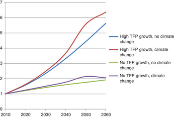
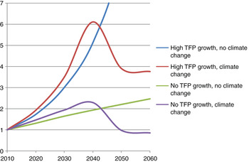
In the moisture-sufficient highlands where cereals dominate, currently accounting for the largest share of agricultural production, crop productivity is projected to increase until approximately 2050 as a result of climate change, but to decline somewhat thereafter; livestock productivity is projected to increase until approximately 2030 as a result of climate change, but to decline sharply thereafter. This is clearly visible in the projected overall production outcomes for crops (figure 1) as well as for livestock (figure 2). Production of both crops and livestock increases faster in the Climate change scenarios than in the corresponding No climate change scenarios until land productivity begins to decline around 2030. In the high TFP growth scenario, the increased overall productivity can compensate for the loss in land productivity until about 2040, but is unable to keep pace with the loss in livestock productivity thereafter, although crop productivity continues to increase. In the low TFP growth scenario, as a result of climate change, production of livestock is lower at the end of the projection period than it is at the beginning.
Value added in crop production in moisture-sufficient cereals-based highlands (Index 2010 = 1)

Value added in livestock production in moisture-sufficient cereals-based highlands (Index 2010 = 1)

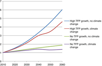
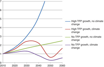
In the drought-prone highlands, the situation is somewhat different. Land productivity in crop production is expected to decline as a result of climate change more or less continuously throughout the period studied. However, the rate of decline increases from the 2030s onwards. There is, therefore, no ‘grace period’ – as in the moisture-sufficient highlands – until 2030, and crop and livestock production both decline continuously compared with the corresponding No climate change scenarios (figures 3 and 4), declining sharply from the 2030s onward.
Value added in crop production in drought-prone highlands (Index 2010 = 1)

Value added in livestock production in drought-prone highlands (Index 2010 = 1)

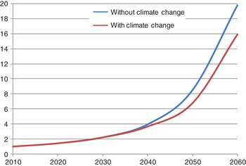
Looking at the implications for the economy as a whole, TFP growth matters more than climate change for the outcomes during the entire period. Nonetheless, climate change has a sizeable impact. Even in the High TFP growth scenario, due to the sharp decline in agriculture after 2030 in the two main farming regions, climate change is projected to have a sizeable impact on the economy (figure 5). Income is projected to increase dramatically in the High TFP growth scenario, but at the end of the simulation period, it is nonetheless some 20 per cent lower than it would have been without climate change.
GDP per capita with high TFP scenarios (Index 2010 = 1)

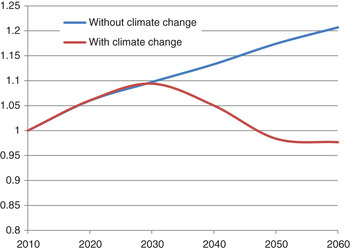
In the No TFP growth scenarios, the outcome is considerably bleaker (figure 6). Since the effects of climate change on agriculture are benign in the main moisture-sufficient regions to begin with, income is projected to increase at roughly the same rate with climate change as it would have without it. However, after the effects of climate change on agriculture start to become negative from 2030 onwards, incomes drop off considerably. At the end of the projected period, because of climate change, average incomes are lower than they are at the beginning of the period – despite the capital accumulation which takes place in the meantime. In the No TFP growth scenario, climate change also leads to a loss of some 20 per cent of income, compared with the No climate change baseline.
GDP per capita with no TFP scenarios (Index 2010 = 1)

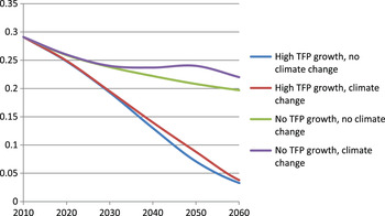
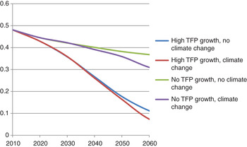
Crop agriculture as a share of GDP shows an overall declining trend over the entire simulation horizon considered in both High TFP and No TFP growth scenarios. The sector declines in absolute terms in the No TFP growth scenario, but its share of the economy nonetheless decreases more slowly in this scenario (figure 7). All agricultural activities as a share of GDP also decline over the entire simulation horizon considered, and decline faster with climate change in both the High TFP and No TFP growth scenarios compared to the No climate change baselines (figure 8).
Crop agriculture as share of GDP

All agricultural activities as share of GDP

5.2. Climate change and growth and poverty reduction
As noted, GDP per capita growth is vastly different in the four different projections. All four income categories studied are hurt considerably by climate change, regardless of the assumption made about TFP growth (see online Appendix table A6). In the No TFP growth scenario, the rural and urban poor are worse off at the end of the simulation period than they are now; poor rural households who mostly produce for their own subsistence gain little from higher relative prices for food and lose from reduced agricultural productivity, while the urban poor lose from higher food prices. In the High TFP growth scenario their per capita income is considerably higher at the end of the projection period than it is now, but almost one-quarter of the income increase seen in the baseline scenario is lost as a result of climate change.
5.3. Comparison with previous studies
Analogously to the other recent Ethiopian CGE studies (Development Prospects Group, 2008; Arndt et al., Reference Arndt, Robinson and Willenbockel2011; Robinson et al., Reference Robinson, Willenbockel and Strzepek2012, Reference Robinson, Strzepek and Cervigni2013) our results indicate that climate change risks having sizeable impacts on the Ethiopian economy. Our results nonetheless differ from theirs in important respects, and it is worthwhile drawing out the implications of these differences.
Our study looks at the impact of changed average weather only, modelling this as a long-term change in the productivity of land and livestock, whereas several of those studies focus on the impacts of changed weather variability, modelling this as annual random shocks to productivity. This means that our modelling approach implicitly assumes that current government efforts to provide stabilization in times of weather shocks, such as the Productive Safety Net Programme (see, for example, Andersson et al., Reference Andersson, Mekonnen and Stage2011), will continue to expand and will provide full asset-smoothing opportunities against weather uncertainty in future, whereas studies that focus on short-term weather variability implicitly assume a return to the older status quo such that no hedging against weather shocks will be available in future. Thus, our model is more sanguine about impacts of climate change in the next few decades but – because of our longer time horizon and the more detailed modelling of long-term productivity decline – even more pessimistic about the decades after that.
An important critique of the Ricardian method (see, for example, Stern, Reference Stern2008) is that the estimates from this method tend to exaggerate the scope for autonomous adaptation outside the range of current climate experiences. Ethiopian agricultural conditions are fairly extreme even by African standards (Von Braun and Webb, Reference Von Braun and Webb1995; World Bank, Reference Bank2008). Hence, all other things equal, a Ricardian analysis based on data from a large range of African agricultural conditions (such as the previous Ethiopian CGE studies cited) will tend to be relatively optimistic about the scope for adaptation to even more extreme weather conditions, whereas a Ricardian analysis based on Ethiopia data only (such as ours, which uses a larger set of survey data from Ethiopia but does not use survey data from other countries) will tend to be less optimistic.
Given these differences in assumptions, modelling approaches and data sources used, it is encouraging that the results remain relatively similar but discouraging that they are so bleak. Both our and other studies indicate that the longer term implications of climate change for Ethiopian agriculture and for the Ethiopian economy as a whole are highly negative.
6. Discussion
Needless to say, modelling the development of the Ethiopian economy over a 50-year period is a formidable task: the country has experienced dramatic swings in economic policy over the past 50 years, and any projections of current trends into the future must be treated with caution. However, a few points from our projection results nonetheless deserve some comment.
TFP growth matters more than climate change for the overall outcome. If current growth trends continue, income levels will rise dramatically over the coming 50 years – despite climate change. If the country returns to the low (or even negative) growth trends experienced in the pre-1992 period, income levels would remain extremely low even if there were no climate change to worry about. This is not surprising in itself, and is analogous to the results from earlier studies.
That being said, climate change does have a dramatic impact – even in the high-growth scenarios. Agriculture currently dominates the country's economy completely, and climate change impacts on agriculture are projected to be considerable in the coming decades. In our study, we assume that it will be possible for farmers to hedge against short-term weather shocks but not against longer term changes in productivity, which is a more optimistic assumption than those made in previous studies. We also assume that factor markets will be sufficiently flexible to permit increased use of other factors such as labour and physical capital in agriculture when land and livestock capital become less productive. Nonetheless, even with these fairly optimistic assumptions, and even with very optimistic assumptions about future growth trends, which would ease the transition of both labour and capital to new agricultural activities and to new activities outside agriculture, there is no way to avoid huge impacts on the overall income level compared with what would have prevailed without climate change. Such a transformation represents a major transition that farmers and private agents will have trouble undertaking on their own, even in a very favourable macroeconomic environment. This huge transition will have to be eased by active adaptation policies on the part of the government, preferably with outside support.