





1. Introduction
Stratified shear flows play a central role in turbulent mixing across a wide range of geophysical and engineering processes. These flows are inherently susceptible to various hydrodynamic instabilities, which facilitate the vertical transport of heat, salt, momentum and biogeochemical tracers across density gradients (e.g. Lévy et al. Reference Lévy, Franks and Smith2018). In the ocean and atmosphere, stratified shear flows regulate exchanges between boundary layers and the interior, thereby influencing large-scale circulation and climate dynamics (e.g. Wunsch & Ferrari Reference Wunsch and Ferrari2004; Stevens & Meneveau Reference Stevens and Meneveau2017; Lévy et al. Reference Lévy, Couespel, Haëck, Keerthi, Mangolte and Prend2024). In industrial and environmental contexts, they govern dispersion and mixing efficiency in stratified reservoirs, estuaries and buoyant outflows (e.g. Farmer & Armi Reference Farmer and Armi1999; Lawrence et al. Reference Lawrence, Pieters, Zaremba, Tedford, Gu, Greco and Hamblin2004; Tedford et al. Reference Tedford, Carpenter, Pawlowicz, Pieters and Lawrence2009). Despite their ubiquity, the interplay between stratification and shear continues to present fundamental challenges, particularly in understanding the transition to turbulence, quantifying irreversible mixing and predicting transport across density interfaces. A mechanistic understanding of such mixing is critical for a broad range of applications, from forecasting saltwater intrusion in estuarine systems to informing subgrid-scale mixing schemes in large-scale ocean circulation models (e.g. Adcroft et al. Reference Adcroft2019; Henson et al. Reference Henson, Laufkötter, Leung, Giering, Palevsky and Cavan2022).
In a stratified system of layers separated by density interfaces, turbulent mixing typically occurs via intermittent, spatially localized events driven by vertical shear across these density interfaces (Sherman et al. Reference Sherman, Imberger and Corcos1978; Ivey et al. Reference Ivey, Winters and Koseff2008; Caulfield Reference Caulfield2021). Turbulent mixing triggered by shear instabilities in stratified flows can be modelled either using forced systems where the flow approaches some kind of quasisteady equilibrium (e.g. Maffioli et al. Reference Maffioli, Brethouwer and Lindborg2016; Lefauve et al. Reference Lefauve, Partridge, Zhou, Dalziel, Caulfield and Linden2018; Howland et al. Reference Howland, Taylor and Caulfield2020; Smith et al. Reference Smith, Caulfield and Taylor2021; Yang et al. Reference Yang, Tedford, Olsthoorn and Lawrence2022a
; Yi & Koseff Reference Yi and Koseff2022; Lewin & Caulfield Reference Lewin and Caulfield2024), or transient systems where the flow is either ‘run-down’/allowed to decay (e.g. Carpenter et al. Reference Carpenter, Lawrence and Smyth2007; Salehipour et al. Reference Salehipour, Caulfield and Peltier2016; de Bruyn Kops & Riley Reference de Bruyn Kops and Riley2019; Fritts et al. Reference Fritts, Wang, Lund and Thorpe2022a
,
Reference Fritts, Wang, Thorpe and Lundb
; Liu et al. Reference Liu, Kaminski and Smyth2022; Riley et al. Reference Riley, Couchman and de Bruyn Kops2023; Yang et al. Reference Yang, Timmermans and Lawrence2024; Petropoulos et al. Reference Petropoulos, de Bruyn Kops and Caulfield2025). Both types of systems have been examined to represent the wide range of natural flow processes associated with environmental and geophysical stratified flows. The mixing properties associated with stratified shear flows depend on a variety of variables such as the initial bulk flow parameters (
 $\textit{Re}$
,
 $\mathit{{Ri}_b}$
and
 $\textit{Pr}$
; defined in § 2) (e.g. Mashayek & Peltier Reference Mashayek and Peltier2012a
,
Reference Mashayek and Peltierb
; VanDine et al. Reference VanDine, Pham and Sarkar2021), the initial level of background turbulence (e.g. Brucker & Sarkar Reference Brucker and Sarkar2007; Kaminski & Smyth Reference Kaminski and Smyth2019; Smith et al. Reference Smith, Caulfield and Taylor2021), the domain length (e.g. Guha & Rahmani Reference Guha and Rahmani2019; Dong et al. Reference Dong, Tedford, Rahmani and Lawrence2019; Liu et al. Reference Liu, Kaminski and Smyth2022), and the shear orientation relative to the background density gradient (e.g. Basak & Sarkar Reference Basak and Sarkar2006; Lucas et al. Reference Lucas, Caulfield and Kerswell2017; Cope et al. Reference Cope, Garaud and Caulfield2020; Yi & Koseff Reference Yi and Koseff2023; Guo et al. Reference Guo, Taylor and Zhou2024).
One of the simplest examples of a stratified shear flow is that of a single sheared density interface. In this configuration, the mixing events are often modelled through canonical stratified shear instabilities such as the Kelvin–Helmholtz (KH) instability (Thorpe Reference Thorpe1971; Caulfield & Peltier Reference Caulfield and Peltier2000; Smyth & Moum Reference Smyth and Moum2012) or the Holmboe instability (Holmboe Reference Holmboe1962; Browand & Winant Reference Browand and Winant1973; Salehipour et al. Reference Salehipour, Caulfield and Peltier2016). The KH instability occurs when the velocity and density interface thicknesses are comparable (
 $R \approx 1$
, where
 $R$
is the ratio of velocity to density interface thickness), producing characteristic stationary overturns or billows. In contrast, Holmboe instability arises when the density interface is much sharper than the velocity shear layer (
 $R \gt 2$
), leading to propagating scouring waves (Alexakis Reference Alexakis2005). Both instability types have been observed in geophysical and laboratory flows. Although natural and experimental shear layers may exhibit varying degrees of asymmetry, where the density interface is offset from the shear layer centre (Zhu & Lawrence Reference Zhu and Lawrence2001; Lefauve et al. Reference Lefauve, Partridge, Zhou, Dalziel, Caulfield and Linden2018; Yang et al. Reference Yang, Tedford, Olsthoorn and Lawrence2022a
), possibly resulting in hybrid forms of KH and Holmboe instabilities (Carpenter et al. Reference Carpenter, Lawrence and Smyth2007; Olsthoorn et al. Reference Olsthoorn, Kaminski and Robb2023; Yang et al. Reference Yang, Timmermans and Lawrence2024), we focus here on symmetric configurations for simplicity. This ensures that the turbulence and associated mixing patterns are symmetric about the interface, enabling a controlled environment for analysing turbulence characteristics, consistent with prior studies (e.g. Caulfield & Peltier Reference Caulfield and Peltier2000; Mashayek & Peltier Reference Mashayek and Peltier2012a
; Salehipour et al. Reference Salehipour, Peltier and Caulfield2018; Kaminski & Smyth Reference Kaminski and Smyth2019; Liu et al. Reference Liu, Kaminski and Smyth2022).
Typically, stratified shear instabilities develop initially as two-dimensional (2-D) primary instabilities, such as KH billows or Holmboe waves. For the KH instability, as the billows grow and reach saturation, they become susceptible to secondary instabilities that lead to a transition into a fully three-dimensional (3-D) turbulent state, marked by intense mixing concentrated near the centre of the shear layer. Eventually, the turbulence decays, and the flow relaminarizes (Mashayek & Peltier Reference Mashayek and Peltier2012a ; Rahmani et al. Reference Rahmani, Lawrence and Seymour2014). For the Holmboe instability, the transition to turbulence occurs when the propagating scouring waves become unstable to secondary perturbations, initiating a breakdown that produces turbulence primarily on either side of the density interface (Smyth & Winters Reference Smyth and Winters2003). Although Holmboe instabilities grow more slowly than KH instabilities, the resulting turbulent mixing tends to be more persistent (Carpenter et al. Reference Carpenter, Lawrence and Smyth2007; Salehipour et al. Reference Salehipour, Caulfield and Peltier2016). The transition of a primarily 2-D flow to 3-D turbulence has been documented in both laboratory experiments (e.g. Thorpe Reference Thorpe1971; Zhu & Lawrence Reference Zhu and Lawrence2001; Yang et al. Reference Yang, Tedford, Olsthoorn and Lawrence2022a ) and field surveys (e.g. Tedford et al. Reference Tedford, Carpenter, Pawlowicz, Pieters and Lawrence2009; Geyer et al. Reference Geyer, Lavery, Scully and Trowbridge2010; Tu et al. Reference Tu, Fan, Sun, Kaminski and Smyth2022; Yeh et al. Reference Yeh, Chang, Lien, Chang, Chen, Jan, Yang and Vladoiu2024).
A common approach to studying these systems is to decompose the flow fields into a background mean state and distinct 2-D and 3-D perturbation components (see figure 1 a and Klaassen & Peltier (Reference Klaassen and Peltier1985), Laprise & Peltier (Reference Laprise and Peltier1989), Smyth & Peltier (Reference Smyth and Peltier1991) and Caulfield & Peltier (Reference Caulfield and Peltier2000)). In a detailed analysis of the transition process, Caulfield & Peltier (Reference Caulfield and Peltier2000) showed that the onset of three-dimensionalization is associated with a marked increase in the rate of mixing. Building on this framework, subsequent studies have investigated how different initial flow configurations affect the instability dynamics and the ensuing mixing (e.g. Carpenter et al. Reference Carpenter, Lawrence and Smyth2007; Salehipour et al. Reference Salehipour, Caulfield and Peltier2016; Caulfield Reference Caulfield2021; Liu et al. Reference Liu, Kaminski and Smyth2022; Yang et al. Reference Yang, Timmermans and Lawrence2024). Despite this progress, the precise mechanisms by which energy is transferred from the one-dimensional (1-D) base state into 2-D flow structures and subsequently into 3-D turbulence remain an open question.
As stratified shear instabilities evolve, the resulting fluid motions disrupt the density field. The energy driving this stirring is partly expended in irreversible mixing and partly in generating internal waves and other reversible motions. Winters et al. (Reference Winters, Lombard, Riley and D’Asaro1995) formalized a method to quantify these contributions by decomposing the total potential energy (PE) into two components: background PE (BPE), which increases due to irreversible mixing, and available PE (APE), which is associated with reversible motions. This framework has become a standard tool for analysing mixing processes in stratified flows (e.g. Caulfield Reference Caulfield2021).
Two different energy exchange schematics of increasing complexity: (a) simple (separation of kinetic energy (KE) into its 1-D, 2-D and 3-D components); (b) complex (further separation of 2-D and 3-D KE into their
 $u$
,
 $v$
and
 $w$
components). Bidirectional arrows indicate physical processes that are not sign definite (though on average they may act either as sources or sinks). Unidirectional arrows indicate sign-definite sources and sinks (e.g. KE dissipation). Here IE stands for internal energy.

Figure 1. Long description
Panel A: A flowchart showing a simple energy exchange schematic with separation of kinetic energy into its 1-D, 2-D, and 3-D components. The diagram includes labeled boxes for IE, K1d, K2d, K3d, APE, BPE, and arrows indicating the flow and interaction between these components. Bidirectional arrows indicate processes that are not sign definite, while unidirectional arrows indicate sign-definite sources and sinks. Panel B: A more complex flowchart further separating 2-D and 3-D kinetic energy into their u, v, and w components. The diagram includes labeled boxes for IE, K1d, K2d,u, K2d,w, K3d,u, K3d,v, K3d,w, R2d,w, R3d,u, R3d,v, R3d,w, APE, BPE, and arrows indicating the flow and interaction between these components. Bidirectional arrows indicate processes that are not sign definite, while unidirectional arrows indicate sign-definite sources and sinks.
In this paper, we further develop the energy budget framework by focusing on the energy redistribution mechanism that connect the different flow components over the course of the flow evolution. By extending the framework of Winters et al. (Reference Winters, Lombard, Riley and D’Asaro1995), we examine the physical processes that precede APE generation by 2-D and 3-D stirring associated with the stratified shear instabilities. We apply our extended theoretical framework to 3-D direct numerical simulations of symmetric KH and Holmboe instabilities to quantify the associated energy transfer and APE generation. The remainder of the paper is organized as follows. Section 2 describes the system set-up and updated frameworks for energy and mixing analyses. We then present results from the 3-D simulations in § 3. Finally, we provide a summary and discussion in § 4.
2. Methodology
Here, we consider a density-stratified shear layer whose initial velocity and density profiles vary in the vertical direction following a hyperbolic tangent function. The velocity distribution has a difference
 $\Delta U^*$
over a length scale
 $h^*$
. Similarly, the stable density distribution has a difference
 $\Delta \rho ^*$
over a length scale
 $\delta ^*$
such that the velocity and density profiles are
 \begin{eqnarray} \overline {U}^* &=& \Delta U^* \,\text{tanh} \left ( \frac {z^*}{h^*} \right )\!, \end{eqnarray}
 \begin{eqnarray} \overline {\rho }^* &=& -\Delta \rho ^*\, \text{tanh}\left (\frac {z^*}{\delta ^*}\right )\!. \end{eqnarray}
The velocity layer thickness is
 $h^* = \Delta U^*/(\text{d}\overline {U}^*/ \text{d}z^*)_{\textit{max}}$
, and the density layer thickness is
 $\delta ^* = \Delta \rho ^*/(\text{d}\overline {\rho }^*/ \text{d}z^*)_{\textit{max}}$
. These idealized, hyperbolic tangent profiles have been used extensively in the literature (e.g. Hazel Reference Hazel1972; Turner Reference Turner1979; Drazin & Reid Reference Drazin and Reid2004; Smyth & Carpenter Reference Smyth and Carpenter2019; Caulfield Reference Caulfield2021), since they closely approximate the background profiles in many natural stratified flows.
Next, we define four dimensionless parameters that characterize the system, which are (i) the Reynolds number (
 $\textit{Re}$
), (ii) the bulk Richardson number (
 $\textit{Ri}_{\textit{b}}$
), (iii) the Schmidt number (
 $\textit{Sc}$
) and (iv) the thickness ratio (
 $R$
), and they are given by
 \begin{align} \textit{Re} &= \frac {\Delta U^* h^*}{\nu ^*}, \\[-12pt]\nonumber \end{align}
 \begin{align} \textit{Ri}_{\textit{b}} &= \frac {\Delta \rho ^* g^* h^*}{\rho _0^* (\Delta U^*)^2}, \\[-12pt]\nonumber \end{align}
 \begin{align} \textit{Sc} &= \frac {\nu ^*}{D^*}, \\[-12pt]\nonumber \end{align}
 \begin{align} R &= \frac {h^*}{\delta ^*}, \\[-12pt]\nonumber \end{align}
where
 $g^*$
is the gravitational acceleration,
 $\rho _0^*$
is a reference density,
 $\nu ^*$
is the kinematic viscosity and
 $D^*$
is the molecular diffusivity of the density field. We define these dimensionless numbers based on the shear interface half-width and half-velocity difference as in previous studies (e.g. Olsthoorn et al. Reference Olsthoorn, Kaminski and Robb2023), while in some studies the full scales are used (e.g. Carpenter et al. Reference Carpenter, Lawrence and Smyth2007).
In this study, we use moderate Reynolds numbers (
 $\textit{Re} = 600$
and 1200), which are comparable to values reported in the recent literature (e.g. Smyth & Moum Reference Smyth and Moum2000b
; Smyth et al. Reference Smyth, Moum and Caldwell2001; Liu et al. Reference Liu, Kaminski and Smyth2022; Olsthoorn et al. Reference Olsthoorn, Kaminski and Robb2023). For reference in dimensional terms, in the case with
 $\textit{Re} = 1200$
, the half-velocity variation is
 $\Delta U^* \approx 6 \times 10^{-3}$
m s
 $^{-1}$
over a length scale of
 $h^* \approx 0.2$
m (Smyth & Moum Reference Smyth and Moum2000b
; Smyth et al. Reference Smyth, Moum and Caldwell2001). The case with
 $\textit{Re} = 600$
represents the same velocity variation over a shorter length scale,
 $h^* \approx 0.1$
m. Similarly, bulk Richardson numbers of
 $\textit{Ri}_{\textit{b}}=$
0.15 and 0.2 are selected. These values of
 $\textit{Re}$
and
 $\textit{Ri}_{\textit{b}}$
are representative of conditions found in laboratory experiments as well as field observations in oceans and lakes (e.g. Thorpe Reference Thorpe1985; Smyth & Moum Reference Smyth and Moum2000b
; Smyth et al. Reference Smyth, Moum and Caldwell2001). We set
 $\textit{Sc}$
= 9, which corresponds to thermally stratified water at approximately 12
 $\,^{\circ }$
C (Sc ranges from 5.5 at 30
 $\,^{\circ }$
C to 13.1 at 0
 $\,^{\circ }$
C; see, e.g. Haigh (Reference Haigh1994)). These parameter values ensure that the turbulence generated by the stratified shear instability reaches a buoyancy Reynolds number (the relative strength of turbulence compared with stratification)
 $\sim O$
(100) (e.g. Smyth & Moum Reference Smyth and Moum2000a
; Smyth et al. Reference Smyth, Moum and Caldwell2001; Olsthoorn et al. Reference Olsthoorn, Kaminski and Robb2023; Yang et al. Reference Yang, Timmermans and Lawrence2024), representative of a wide range of flows in estuaries, oceans and lakes (e.g. Monismith et al. Reference Monismith, Koseff and White2018; Dosser et al. Reference Dosser, Chanona, Waterman, Shibley and Timmermans2021; Sepúlveda Steiner et al. Reference Sepúlveda Steiner, Forrest, McInerney, Fernández Castro, Lavanchy, Wüest and Bouffard2023). We set
 $R = h^*/\delta ^* = 1$
in this study, such that the flow is susceptible to the KH instability, an inviscid mode whose growth rate decreases monotonically with increasing ambient stratification. At finite amplitude, this instability manifests as an array of elliptical vortices or billows which ‘roll up’ or ‘overturn’ the density interface. Additionally, we set
 $R = 3$
, such that the flow is susceptible to the Holmboe instability. It has recently been appreciated that Holmboe instability is another important mechanism characterized by counter-propagating internal waves that generate the relatively long-lived turbulence (e.g. Salehipour et al. Reference Salehipour, Caulfield and Peltier2016; Salehipour & Peltier Reference Salehipour and Peltier2019).
Our computational set-up and flow parameters have been chosen to prioritize the study of dynamics in aquatic environments (
 $\textit{Sc} \gt 1$
), and with
 $\textit{Sc} = 9$
, a simulation with
 $\textit{Re}=1200$
requires approximately 172 000 central processing unit hours, placing a computational constraint on exploring larger values of
 $\textit{Re}$
. Furthermore, our choice of
 $\textit{Ri}_{\textit{b}}$
,
 $\textit{Sc}$
and
 $R$
allows for more direct comparison with previous studies (e.g. Smyth & Winters Reference Smyth and Winters2003; Carpenter et al. Reference Carpenter, Lawrence and Smyth2007; Olsthoorn et al. Reference Olsthoorn, Kaminski and Robb2023; Yang et al. Reference Yang, Timmermans and Lawrence2024). A total of seven numerical experiments are performed with various parameters (see table 1), and hereafter, all quantities are dimensionless and are denoted without asterisks.
Numerical experiments presented in this study including their parameters. We consider both
 $R = 1$
for KH profiles (cases 0
 $-$
3) and
 $R = 3$
for Holmboe profiles (cases 4
 $-$
6). All simulations have
 $\textit{Sc} = 9$
.

Table 1. Long description
The table presents six numerical experiments with varying parameters for KH and Holmboe profiles. It includes columns for case number, instability type, domain size, resolution, and three dimensionless numbers: R, Re, and Rib. The table has seven columns: Case, Instability, Domain size, Resolution, R, Re, and Rib. The domain size is given in units of Lx, Ly, and Lz, while the resolution is given in units of Nx, Ny, and Nz. The table lists the following data: Row 1: Case 0, Instability KH, Domain size 14.0 x 18 x 18, Resolution 768 x 1024 x 1024, R 1, Re 1200, Rib 0.15. Row 2: Case 1, Instability KH, Domain size 14.0 x 9 x 18, Resolution 768 x 512 x 1024, R 1, Re 1200, Rib 0.15. Row 3: Case 2, Instability KH, Domain size 13.4 x 9 x 18, Resolution 768 x 512 x 1024, R 1, Re 1200, Rib 0.20. Row 4: Case 3, Instability KH, Domain size 14.0 x 9 x 18, Resolution 512 x 384 x 768, R 1, Re 600, Rib 0.15. Row 5: Case 4, Instability Holmboe, Domain size 15.5 x 9 x 18, Resolution 768 x 512 x 1024, R 3, Re 1200, Rib 0.20. Row 6: Case 5, Instability Holmboe, Domain size 13.7 x 9 x 18, Resolution 768 x 512 x 1024, R 3, Re 1200, Rib 0.20. Row 7: Case 6, Instability Holmboe, Domain size 15.8 x 9 x 18, Resolution 512 x 384 x 768, R 3, Re 600, Rib 0.15.
The evolution of the velocity
 $u_{\!j}$
and density
 $\rho$
fields are described by the non-dimensional Navier–Stokes equations under the Boussinesq approximation,
 \begin{align} \partial _{\!j} u_{\!j} &= 0, \\[-12pt]\nonumber \end{align}
 \begin{align} \partial _{t} u_{\!j} + u_{m} \partial _{m} u_{\!j} &= -\partial _{\!j} p - \textit{Ri}_{\textit{b}} \rho \delta _{j3} +\textit{Re}^{-1} \partial _{m} \partial _{m} u_{\!j}, \\[-12pt]\nonumber \end{align}
 \begin{align} \partial _{t} \rho + u_{m} \partial _{m} \rho &= (\textit{Re Sc})^{-1} \partial _{m} \partial _{m} \rho, \end{align}
where
 $p$
is the pressure field and
 $\delta _{j3}$
denotes a unit vector in the vertical direction. We apply the following tensor notation conventions in this work: (i) we reserve the index
 $t$
for the time coordinate; (ii) indices in the subscripts (such as
 $j$
and
 $m$
) are free indices, taking values
 $1, 2, 3$
with the values corresponding to the
 $x$
,
 $y$
,
 $z$
directions, respectively; and (iii) repeated indices imply summation.
We solve the non-dimensional Navier–Stokes (2.7)–(2.9) using a direct numerical simulation codebase called SPINS (spectral parallel incompressible Navier–Stokes solver (Subich et al. Reference Subich, Lamb and Stastna2013)). The streamwise domain length is set to
 $L_x = \lambda _x$
, corresponding to the wavelength of the most unstable linear mode. The spanwise extent of the domain is
 $L_y = 9$
, which exceeds
 $L_x/2$
and is sufficient to allow the development of 3-D secondary instabilities (e.g. Caulfield & Peltier Reference Caulfield and Peltier2000; Smyth & Winters Reference Smyth and Winters2003; Carpenter et al. Reference Carpenter, Lawrence and Smyth2007; Mashayek & Peltier Reference Mashayek and Peltier2013; Salehipour et al. Reference Salehipour, Peltier and Caulfield2018; Lewin & Caulfield Reference Lewin and Caulfield2022). We carry out an additional KH simulation for
 $\textit{Re}=1200$
and
 $\textit{Ri}_{\textit{b}} = 0.15$
with a doubled spanwise domain,
 $L_y =$
18 (Case 0), to test for spanwise confinement effects. We note minimal differences between the two simulations (see Appendix D). The vertical domain height is
 $L_z = 18$
, chosen to ensure that vertical boundary effects have a negligible influence on the instability dynamics (e.g. Haigh & Lawrence Reference Haigh and Lawrence1999; Carpenter et al. Reference Carpenter, Lawrence and Smyth2007; Olsthoorn et al. Reference Olsthoorn, Kaminski and Robb2023). Periodic boundary conditions are imposed in the horizontal directions, while free-slip and no-flux conditions are applied at the upper and lower boundaries. The grid spacing is chosen to be less than three times the minimum Batchelor scale (Olsthoorn et al. Reference Olsthoorn, Kaminski and Robb2023),
 $L_B = L_K/\textit{Sc}^{1/2}$
, where
 $L_K = (\nu ^3/\epsilon )^{1/4}$
is the Kolmogorov length scale and
 $\epsilon$
is the viscous dissipation rate (Moin & Mahesh Reference Moin and Mahesh1998; Arthur & Fringer Reference Arthur and Fringer2014), which ensures that the mixing and turbulence statistics are insensitive to grid resolution (see figure 8e of Kaminski & Smyth Reference Kaminski and Smyth2019).
2.1. Energy analysis
In figure 1, we present two different schematics that illustrate the energy exchange processes in stratified shear layers. The first schematic illustrates a classical picture that only involves the separation of KE into its 1-D, 2-D and 3-D components (figure 1
a). The 1-D component is obtained by averaging the flow in the
 $x$
and
 $y$
directions
 $f_{1d}(z,t) = \langle f(\boldsymbol{x},t) \rangle _{x,y}$
, where
 $f$
can be replaced with any flow variable of interest, such as the horizontal velocity; the 2-D component of the flow variables is found by averaging the equations in the
 $y$
direction (e.g.
 $f_{2d}(x,z,t) = \langle f(\boldsymbol{x},t) \rangle _{y} - f_{1d}(z,t)$
); and the remaining part is the 3-D component (see further details in Appendix A and also in Caulfield & Peltier (Reference Caulfield and Peltier2000) and Peltier & Caulfield (Reference Peltier and Caulfield2003)). The second schematic presents a further breakdown of the 2-D and 3-D KE into their
 $u$
,
 $v$
and
 $w$
components (figure 1
b). For example when
 $f(\boldsymbol{x},t) = u(\boldsymbol{x},t), v(\boldsymbol{x},t),$
or
 $w(\boldsymbol{x},t)$
, the 1-D, 2-D and 3-D components of KE are defined as
 $K_{1d} =({1}/{2})\langle u_{1d} u_{1d}\rangle _{z}$
,
 $K_{2d} = K_{2d,u} + K_{2d,w} = ({1}/{2}) \langle u_{2d} u_{2d}\rangle _{x,z} +({1}/{2})\langle w_{2d} w_{2d}\rangle _{x,z}$
and
 $K_{3d} = K_{3d,u} + K_{3d,v} + K_{3d,w} = ({1}/{2}) \langle u_{3d} u_{3d}\rangle _{x,y,z} + ({1}/{2}) \langle v_{3d} v_{3d}\rangle _{x,y,z} + ({1}/{2}) \langle w_{3d} w_{3d}\rangle _{x,y,z}$
(see further details in Appendix A).
The classical picture reveals physical processes that facilitate the exchange of KE associated with the 1-D, 2-D and 3-D motions, each of which is represented through bidirectional arrows that connect the three different coloured boxes (i.e.
 $P_{1d\leftrightarrow 2d}$
,
 $P_{1d\leftrightarrow 3d}$
,
 $P_{2d\leftrightarrow 3d}$
, which are shear production terms exchanging energy between different flow dimensions; they will be defined more explicitly in the next section). Comparing figures 1(a) and 1(b), the further breakdown of 2-D and 3-D KE into their
 $u$
,
 $v$
and
 $w$
components reveal the integral role of pressure–strain redistribution processes, each of which is presented through bidirectional arrows between the components of
 $K_{2d}$
and
 $K_{3d}$
(i.e.
 $R_{2d,u}$
,
 $R_{2d,w}$
,
 $R_{3d,u}$
,
 $R_{3d,v}$
and
 $R_{3d,w}$
), for the generation of 2-D and 3-D motions and their subsequent role in the generation of APE through the 2-D and 3-D stirring processes (i.e.
 $B_{2d}$
and
 $B_{3d}$
). Considering the generation of
 $K_{2d}$
in figure 1(b), it can be seen that
 $K_{1d}$
is only exchanged directly with the
 $u$
-component of
 $K_{2d}$
, and the generation of the
 $w$
-component of
 $K_{2d}$
occurs via pressure–strain redistribution. Additionally, considering now the generation of
 $K_{3d}$
, we observe that the
 $u$
-component of
 $K_{3d}$
can be directly generated via exchange with
 $K_{1d}$
and
 $K_{2d,u}$
and that the
 $w$
-component of
 $K_{3d}$
can be directly generated via exchange with
 $K_{2d,w}$
. Contrary to these two components, the
 $v$
-component of
 $K_{3d}$
, does not have a direct generation mechanism connected with 1-D and 2-D motions, and relies solely on 3-D pressure–strain redistribution to be generated. While
 $K_{3d,u}$
and
 $K_{3d,w}$
too can be indirectly generated via pressure–strain redistribution, these components have direct production mechanisms, making it more likely that the pressure-strain redistribution will take energy from them to generate
 $K_{3d,v}$
(this idea is at the heart of Rotta’s return-to-isotropy hypothesis and the related Reynolds stress evolution model (Rotta Reference Rotta1951)). Finally, the detailed breakdown of the 2-D and 3-D KE helps us explore different pathways of APE generation of stratified shear layer systems. Reversible APE generation occurs either through 2-D or 3-D stirring (
 $B_{2d}$
or
 $B_{3d}$
), and the energy exchange diagram in figure 1(b) reveals various pathways through which
 $K_{1d}$
can eventually be converted into
 $K_{2d,w}$
and
 $K_{3d,w}$
for access by
 $B_{2d}$
or
 $B_{3d}$
. We note that APE generation through 2-D or 3-D stirring must first occur before any irreversible mixing of APE into BPE can take place.
An illustration of the pressure–strain redistribution process converting
 $K_{u}$
into
 $K_{w}$
, where redistribution is driven by either (a) horizontal convergence or (b) horizontal divergence with subsequent pressure fluctuations that are generated to satisfy the continuity equation. The blue dots represent fluid parcels and the arrows denote their movement.

To illustrate the physical mechanism that facilitates the conversion of energy among the
 $u$
,
 $v$
and
 $w$
components of
 $K_{2d}$
and
 $K_{3d}$
, we introduce a schematic of the pressure–strain redistribution (figure 2). This conversion occurs between
 $K_{2d,u}$
and
 $K_{2d,w}$
and among
 $K_{3d,u}$
,
 $K_{3d,v}$
and
 $K_{3d,w}$
, but not between the 2-D and 3-D components. Recall from figure 1(b) how
 $K_{2d,w}$
and
 $K_{3d,v}$
lack direct generation terms that convert
 $K_{1d}$
, indicating the need for another source term in order for these components to become finite in time. In figure 2, we consider two scenarios driven by either horizontal convergence (figure 2
a) or horizontal divergence (figure 2
b). Horizontal convergence drives a high-pressure perturbation at the centre that is associated with a vertical divergence in order to satisfy the continuity equation. Horizontal divergence drives a low-pressure perturbation at the centre that is associated with a vertical convergence in order to satisfy the continuity equation. Both scenarios lead to a negative correlation between
 $p'$
and
 $\partial _{x} u'$
but a positive correlation between
 $p'$
and
 $\partial _{z} w'$
, resulting in a conversion of the
 $u$
-component of KE into the
 $w$
-component of KE.
In the following sections, we derive the volume-averaged equations for the various components of KE as well as the 2-D and 3-D stirring processes (
 $B_{2d}$
and
 $B_{3d}$
) that are illustrated in figure 1(b) and study their time-varying contributions to determine which of the various APE generation pathways contribute most significantly to the eventual irreversible mixing of APE into BPE in the stratified sheared systems we consider in this work.
2.2. Volume-averaged KE and stirring budgets
Here, we arrive at the 1-D, 2-D and 3-D KE equations by multiplying (A2), (A5) and (A8) by
 $u_{j,1d}$
,
 $u_{j,\mathrm{ 2d}}$
,
 $u_{j,{3d}}$
, respectively, and applying a volume average. The vertical transport terms disappear after vertical averaging due to the top and bottom boundary conditions. The volume-averaged 1-D, 2-D and 3-D KE equations are
 \begin{align} \partial _{t} K_{1d} &= \underbrace {\langle \langle u_{2d} w_{2d} \rangle _{x} \partial _{z} u_{1d} \rangle _{z}}_{-P_{1d \leftrightarrow 2d,u}} + \underbrace {\langle \langle u_{3d} w_{3d} \rangle _{x,y} \partial _{z} u_{1d} \rangle _{z}}_{-P_{1d \leftrightarrow 3d,u}} -\underbrace {\frac {1}{\textit{Re}} \langle \partial _{z} u_{1d} \partial _{z} u_{1d} \rangle _{z}}_{\epsilon _{1d}}, \\[-12pt]\nonumber\end{align}
 \begin{align} \partial _{t} K_{2d} &= \underbrace {-\langle \langle u_{2d} w_{2d} \rangle _{x} \partial _{z} u_{1d} \rangle _{z}}_{P_{1d \leftrightarrow 2d,u}} + \underbrace {\langle \langle u_{j,{3d}} u_{m,{3d}} \rangle _{y} \partial _{m} u_{j,{2d}} \rangle _{x,z}}_{-P_{2d \leftrightarrow 3d}} \nonumber \\ &\, - \underbrace {\mathit{Ri_b} \langle w_{{2d}} \rho _{{2d}} \rangle _{x,z}}_{B_{2d}} -\underbrace {\frac {1}{\textit{Re}} \langle \partial _{m} u_{j,{2d}} \partial _{m} u_{j,{2d}} \rangle _{x,z}}_{\epsilon _{2d}}, \\[-12pt]\nonumber \end{align}
 \begin{align} \partial _{t} K_{3d} &= \underbrace {-\langle \langle u_{3d} w_{3d} \rangle _{x,y} \partial _{z} u_{1d} \rangle _{z}}_{P_{1d \leftrightarrow 3d,u}} \underbrace {-\langle \langle u_{j,{3d}} u_{m,{3d}} \rangle _{y} \partial _{m} u_{j,{2d}} \rangle _{x,z}}_{P_{2d \leftrightarrow 3d}} \nonumber \\ &\, -\underbrace {\mathit{Ri_b} \langle w_{3d} \rho _{3d} \rangle _{x,y,z}}_{B_{3d}} -\underbrace {\frac {1}{\textit{Re}} \langle \partial _{m} u_{j,{3d}} \partial _{m} u_{j,{3d}} \rangle _{x,y,z}}_{\epsilon _{3d}}. \end{align}
Here, we introduce additional tensor notation conventions that will apply throughout the work: (i) we reserve the indices
 $x, y, z$
for the three spatial coordinates, and
 $u, v, w$
for their corresponding velocity components; and (ii)
 $1d, 2d, 3d$
in the subscripts denote the dimension of the flow field. Equations (2.10)–(2.12) correspond to the simpler energy exchange diagram in figure 1(a), and
 $P_{2d \leftrightarrow 3d} = P_{2d,u \leftrightarrow 3d,u} + P_{2d,w \leftrightarrow 3d,w}$
(see figure 1
b). Additionally, by summing (2.10)–(2.12), we arrive at the evolution equation for the total KE
 $K = K_{1d} + K_{2d} + K_{3d}$
,
 \begin{align} d_{t} K &= -\underbrace {\mathit{Ri_b} \langle w \rho \rangle _{x,y,z}}_{B} -\underbrace {\frac {1}{\textit{Re}} \langle \partial _{m} u_{\!j} \partial _{m} u_{\!j} \rangle _{x,y,z}}_{\epsilon } \nonumber \\ &= - \underbrace {\mathit{Ri_b} \langle w_{{2d}} \rho _{{2d}} \rangle _{x,z}}_{B_{2d}} \, -\underbrace {\mathit{Ri_b} \langle w_{3d} \rho _{3d} \rangle _{x,y,z}}_{B_{3d}} \nonumber \\ & -\underbrace {\frac {1}{\textit{Re}} \langle \partial _{z} u_{1d} \partial _{z} u_{1d} \rangle _{z}}_{\epsilon _{1d}} \, -\underbrace {\frac {1}{\textit{Re}} \langle \partial _{m} u_{j,{2d}} \partial _{m} u_{j,{2d}} \rangle _{x,z}}_{\epsilon _{2d}} \nonumber \\ &-\underbrace {\frac {1}{\textit{Re}} \langle \partial _{m} u_{j,{3d}} \partial _{m} u_{j,{3d}} \rangle _{x,y,z}}_{\epsilon _{3d}}, \end{align}
which shows that reversible exchange between the total KE and APE occurs via 2-D and 3-D stirring processes (i.e.
 $B = B_{2d} + B_{3d}$
), and that irreversible loss of total KE occurs through the three viscous dissipation terms associated with the 1-D, 2-D and 3-D flow components (
 $\epsilon = \epsilon _{1d} + \epsilon _{2d} + \epsilon _{3d}$
) as well as irreversible mixing of APE into BPE (
 $M_{i}$
). The overall process is presented in figure 1(a) and the literature (see figure 2 of Winters et al. (Reference Winters, Lombard, Riley and D’Asaro1995), figure 2 of Caulfield & Peltier (Reference Caulfield and Peltier2000) and figure 4 of Carpenter et al. (Reference Carpenter, Lawrence and Smyth2007) for prior depictions of the energy exchange in stratified shear flows).
Note that in the above equations, the dissipation rates are defined using the full velocity gradient tensor rather than the strain-rate tensor (its symmetric component). In this work, we will work with the pseudodissipation rate (i.e. dissipation rate defined using the full velocity gradient tensor) and denote it using
 $\epsilon$
in contrast to the true dissipation rate,
 $\epsilon _{\textit{T}}$
, (i.e. dissipation rate defined using the strain-rate tensor). In Appendix B, we theoretically demonstrate the equivalence of the two sets of dissipation definitions under volume averaging for
 $K_{1d}$
,
 $K_{2d}$
and
 $K_{3d}$
(i.e.
 $\langle \epsilon _{1d} \rangle _{x,y,z} = \langle \epsilon _{\textit{T},1\textit{d}} \rangle _{x,y,z}$
,
 $\langle \epsilon _{2d} \rangle _{x,y,z} = \langle \epsilon _{\textit{T},2\textit{d}} \rangle _{x,y,z}$
and
 $\langle \epsilon _{3d} \rangle _{x,y,z} = \langle \epsilon _{\textit{T},3\textit{d}} \rangle _{x,y,z}$
), and we also discuss additional terms that arise when considering the
 $u$
,
 $v$
and
 $w$
components of the KE separately.
In order to arrive at a more detailed understanding of the physical processes involved in KE and APE generation and the eventual irreversible mixing of APE into BPE, we further decompose the 2-D and 3-D KE components into their constituents (
 $K_{2d} = K_{2d,u} + K_{2d,w}$
and
 $K_{3d} = K_{3d,u} + K_{3d,v} + K_{3d,w})$
. Beginning with the 2-D momentum equations (A5), we arrive at the volume-averaged evolution equations for
 $K_{2d,u}$
and
 $K_{2d,w}$
as
 \begin{align} \partial _{t} K_{2d,u} = \partial _{t} \left ( \frac {1}{2} \langle u_{2d} u_{2d} \rangle _{x,z} \right ) &= \underbrace {-\langle \langle u_{2d} w_{2d} \rangle _{x} \partial _{z} u_{1d} \rangle _{z}}_{P_{1d \leftrightarrow 2d,u}} + \underbrace {\langle \langle u_{{3d}} u_{m,{3d}} \rangle _{y} \partial _{m} u_{{2d}} \rangle _{x,z}}_{-P_{2d,u \leftrightarrow 3d,u}}\nonumber \\ &+ \underbrace {\langle p_{2d} \partial _{x} u_{2d} \rangle _{x,z}}_{R_{2d,u}} -\underbrace {\frac {1}{\textit{Re}} \langle \partial _{m} u_{2d} \partial _{m} u_{2d} \rangle _{x,z}}_{\epsilon _{2d,u}}, \\[-12pt]\nonumber \end{align}
 \begin{align} \partial _{t} K_{2d,w} =\partial _{t} \left ( \frac {1}{2} \langle w_{2d} w_{2d} \rangle _{x,z} \right ) &= \underbrace {\langle p_{2d} \partial _{z} w_{2d} \rangle _{x,z}}_{R_{2d,w}} + \underbrace {\langle \langle w_{{3d}} u_{m,{3d}} \rangle _{y} \partial _{m} w_{{2d}} \rangle _{x,z}}_{-P_{2d,w \leftrightarrow 3d,w}} \nonumber \\ &-\underbrace {\mathit{Ri_b} \langle w_{2d} \rho _{2d} \rangle _{x,z}}_{B_{2d}} -\underbrace {\frac {1}{\textit{Re}} \langle \partial _{m} w_{2d} \partial _{m} w_{2d} \rangle _{x,z}}_{\epsilon _{2d,w}}. \end{align}
These two equations also demonstrate that the shear-production term only facilitates conversion of
 $K_{1d}$
into
 $K_{2d,u}$
. In order for
 $K_{2d,w}$
to be generated, the 2-D pressure–strain redistribution terms must convert
 $K_{2d,u}$
into
 $K_{2d,w}$
, where the sum of the two pressure–strain redistribution terms is zero (
 $R_{2d,u} + R_{2d,w} = 0$
) by the 2-D continuity equation, (A4). Note that the sum of (2.14) and (2.15) recovers (2.11). In addition, (2.15) reveals that reversible exchange between KE and APE occurs through the 2-D vertical buoyancy flux term, which connects
 $K_{2d,w}$
and APE. Therefore, the volume-averaged energy evolution equations presented thus far reveal the first pathway of APE generation, which involves the following energy conversion processes: (i) conversion of
 $K_{1d}$
to
 $K_{2d,u}$
through a shear production term (
 $P_{1d \leftrightarrow 2d,u} = -\langle \langle u_{2d} w_{2d} \rangle _{x} \partial _{z} u_{1d} \rangle _{z}$
); (ii) conversion of
 $K_{2d,u}$
to
 $K_{2d,w}$
through the 2-D pressure–strain redistribution (
 $R_{2d,w} = \langle p_{2d} \partial _{z} w_{2d} \rangle _{x,z}= -\langle p_{2d} \partial _{x} u_{2d} \rangle _{x,z} = -R_{2d,u}$
); (iii) conversion of
 $K_{2d,w}$
to APE through the 2-D vertical buoyancy flux (
 $B_{2d} = \mathit{Ri_b} \langle w_{2d} \rho _{2d} \rangle _{x,z}$
).
Next, we begin with the 3-D momentum equations (A8) and arrive at the volume-averaged evolution equations for
 $K_{3d,u}$
,
 $K_{3d,v}$
and
 $K_{3d,w}$
as
 \begin{align} \partial _{t} K_{3d,u} =\partial _{t} \left ( \frac {1}{2} \langle u_{3d} u_{3d} \rangle _{x,y,z} \right ) &= \underbrace {-\langle \langle u_{3d} w_{3d} \rangle _{x,y} \partial _{z} u_{1d} \rangle _{z}}_ {P_{1d \leftrightarrow 3d,u}} \underbrace {-\langle \langle u_{{3d}} u_{m,{3d}} \rangle _{y} \partial _{m} u_{{2d}} \rangle _{x,z}}_{P_{2d,u \leftrightarrow 3d,u}}\nonumber \\ &+ \underbrace {\langle p_{3d} \partial _{x} u_{3d} \rangle _{x,y,z}}_{R_{3d,u}} -\underbrace {\frac {1}{\textit{Re}} \langle \partial _{m} u_{3d} \partial _{m} u_{3d} \rangle _{x,y,z}}_{\epsilon _{3d,u}}, \\[-12pt]\nonumber \end{align}
 \begin{align} \partial _{t} K_{3d,v} = \partial _{t} \left ( \frac {1}{2} \langle v_{3d} v_{3d} \rangle _{x,y,z} \right ) &= \underbrace {\langle p_{3d} \partial _{y} v_{3d} \rangle _{x,y,z}}_{R_{3d,v}} -\underbrace {\frac {1}{\textit{Re}} \langle \partial _{m} v_{3d} \partial _{m} v_{3d} \rangle _{x,y,z}}_{\epsilon _{3d,v}}, \end{align}
 \begin{align} \partial _{t} K_{3d,w} = \partial _{t} \left ( \frac {1}{2} \langle w_{3d} w_{3d} \rangle _{x,y,z} \right ) &= \underbrace {\langle p_{3d} \partial _{z} w_{3d} \rangle _{x,y,z}}_{R_{3d,w}} \underbrace {-\langle \langle w_{{3d}} u_{m,{3d}} \rangle _{y} \partial _{m} w_{{2d}} \rangle _{x,z}}_{P_{2d,w \leftrightarrow 3d,w}}\nonumber \\ &-\underbrace {\mathit{Ri_b} \langle w_{3d} \rho _{3d} \rangle _{x,y,z}}_{B_{3d}} -\underbrace {\frac {1}{\textit{Re}} \langle \partial _{m} w_{3d} \partial _{m} w_{3d} \rangle _{x,y,z}}_{\epsilon _{3d,w}}. \end{align}
These three equations demonstrate that
 $K_{3d,u}$
can be generated through exchange with
 $K_{1d}$
and
 $K_{2d,u}$
and that
 $K_{3d,w}$
can be generated through exchange with
 $K_{2d,w}$
. The spanwise component (
 $K_{3d,v}$
), however, depends solely on the pressure–strain redistribution for growth, since the only other term is viscous dissipation, which is a sink. Note that the sum of (2.16)–(2.18) recovers (2.12). In addition, (2.18) reveals that reversible exchange between KE and APE can additionally occur through the 3-D buoyancy flux, which connects
 $K_{3d,w}$
and APE. Therefore, the three volume-averaged energy evolution equations associated with
 $K_{3d}$
indicate a second set of pathways of APE generation in parallel stratified shear flows, which involves (i) the generation of
 $K_{3d,w}$
through a variety of different physical processes (see figure 1
b) and (ii) the conversion
 $K_{3d,w}$
into APE through the 3-D buoyancy flux (
 $B_{3d} = \mathit{Ri_b} \langle w_{3d} \rho _{3d} \rangle _{x,y,z}$
). The importance of this second set of APE generation pathways depends on how effectively
 $K_{3d,w}$
is generated through the various exchange processes as well as how effectively
 $K_{3d,w}$
is then converted into APE.
2.3. Mixing analysis
Related to the various components of KE that we have discussed in the previous section, we note that 2-D and 3-D buoyancy fluxes convert
 $K_{2d,w}$
and
 $K_{3d,w}$
into APE. Some of the APE gets converted back into
 $K_{2d,w}$
and
 $K_{3d,w}$
since
 $B_{2d}$
and
 $B_{3d}$
are reversible processes, but there is irreversible transfer of some of the APE into BPE by
 $M_{i}$
. In this section, we present the volume-averaged evolution of 2-D and 3-D vertical buoyancy fluxes to directly determine which physical processes are responsible for the strengthening or weakening of the 2-D and 3-D reversible stirring that facilitates the exchanges between
 $K_{2d,w}$
,
 $K_{3d,w}$
and APE.
2.3.1. Vertical buoyancy flux budgets
Here, we present the volume-averaged, 2-D and 3-D vertical buoyancy flux (
 ${B}_{2d}$
and
 $B_{3d}$
) evolution equations, which we arrive at by manipulating (A5) and (A6) and (A8) and (A9),
 \begin{align} \partial _{t} \underbrace {\mathit{Ri_b}\langle w_{2d} \rho _{2d} \rangle _{x,z}}_ {B_{2d}} &= \underbrace {-\mathit{Ri_b}\langle \langle w_{2d} w_{2d} \rangle _{x} \partial _{z} \rho _{1d} \rangle _{z}}_{P^{(1)}_{2d,{B}}} \nonumber \\ &+ \underbrace {\mathit{Ri_b}\langle \langle u_{m,{3d}} w_{3d} \rangle _{y} \partial _{m} \rho _{2d} \rangle _{x,z}}_{-P^{(2)}_{3d,{B}}} + \underbrace {\mathit{Ri_b}\langle \langle u_{m,{3d}} \rho _{3d} \rangle _{y} \partial _{m} w_{2d} \rangle _{x,z}}_{-P^{(3)}_{3d,{B}}} \nonumber \\ &+ \underbrace {\mathit{Ri_b}\langle p_{2d} \partial _{z} \rho _{2d} \rangle _{x,z}}_{R_{2d,{B}}} - \underbrace {\mathit{Ri_b}^{2} \langle \rho _{2d} \rho _{2d} \rangle _{x,z}}_{D_{2d,{B}}} \nonumber \\ &- \underbrace {\mathit{Ri_b} \left ( \frac {1}{\textit{Re}} + \frac {1}{\textit{Re Sc}} \right ) \langle \partial _{m} w_{2d} \partial _{m} \rho _{2d} \rangle _{x,z}}_{\epsilon _{2d,{B}}}, \\[-12pt]\nonumber \end{align}
 \begin{align} \partial _{t} \underbrace {\mathit{Ri_b} \langle w_{3d} \rho _{3d} \rangle _{x,y,z}}_{B_{3d}} &= \underbrace {-\mathit{Ri_b} \langle \langle w_{3d} w_{3d} \rangle _{x,y} \partial _{z} \rho _{1d} \rangle _{z}}_{P^{(1)}_{3d,{B}}} \nonumber \\ & \underbrace {-\mathit{Ri_b} \langle \langle u_{m,{3d}} w_{3d} \rangle _{y} \partial _{m} \rho _{2d} \rangle _{x,z}}_{P^{(2)}_{3d,{B}}} \underbrace {-\mathit{Ri_b}\langle \langle u_{m,{3d}} \rho _{3d} \rangle _{y} \partial _{m} w_{2d} \rangle _{x,z}}_{P^{(3)}_{3d,{B}}} \nonumber \\ &+ \underbrace {\mathit{Ri_b} \langle p_{3d} \partial _{z} \rho _{3d} \rangle _{x,y,z}}_{R_{3d,{B}}} -\underbrace {\mathit{Ri_b}^{2} \langle \rho _{3d} \rho _{3d} \rangle _{x,y,z}}_{D_{3d,{B}}} \nonumber \\ &-\underbrace {\mathit{Ri_b} \left (\frac {1}{\textit{Re}} + \frac {1}{\textit{Re Sc}} \right ) \langle \partial _{m} w_{3d} \partial _{m} \rho _{{3d}} \rangle _{x,y,z}}_{\epsilon _{3d,{B}}}. \end{align}
In figure 3, we illustrate the sources and sinks of
 $B_{2d}$
and
 $B_{3d}$
from the perspective of down-gradient fluxes (i.e.
 $B_{2d}, B_{3d} \gt 0$
). For
 $B_{2d}$
, which facilitates the reversible exchange between
 $K_{2d,w}$
and APE, there is generation of
 $B_{2d}$
by a term that is proportional to
 $K_{2d,w}$
(
 $P_{2d,B}^{(1)}$
) and destruction of
 $B_{2d}$
by a term that is proportional to
 $\rho _{2d}^{2}$
(
 $D_{2d,B})$
. The 2-D vertical pressure scrambling (correlation between the pressure and vertical density gradient;
 $R_{2d,B}$
) and small-scale destruction terms (
 $\epsilon _{2d,B}$
) are sign indefinite, and can either help strengthen or weaken the reversible exchange between
 $K_{2d,w}$
and APE. For
 $B_{3d}$
, which facilitates the reversible exchange between
 $K_{3d,w}$
and APE, there is generation of
 $B_{3d}$
by a term that is proportional to
 $K_{3d,w}$
(
 $P_{3d,B}^{(1)}$
) and destruction of
 $B_{3d}$
by a term that is proportional to
 $\rho _{3d}^{2}$
(
 $D_{3d,B}$
). The 3-D vertical pressure scrambling (
 $R_{3d,B}$
) and small-scale destruction terms (
 $\epsilon _{3d,B}$
) are sign indefinite, and can either strengthen or weaken the reversible exchange between
 $K_{3d,w}$
and APE. Lastly, we note that there are two sets of terms that facilitate direct exchange between
 $B_{2d}$
and
 $B_{3d}$
that depend on the correlation of the 3-D buoyancy fluxes with gradients of
 $w_{2d}$
(
 $P_{3d,B}^{(3)}$
) and the correlation of the 3-D Reynolds stresses with gradients of
 $\rho _{2d}$
(
 $P_{3d,B}^{(2)}$
).
A schematic of the sources and sinks of 2-D and 3-D vertical buoyancy fluxes associated with (2.19) and (2.20). Bidirectional arrows indicate terms that are not sign definite (though on average they may act either as sources and sinks), and unidirectional arrows indicate terms that are sign definite from the perspective of sources and sinks of down-gradient fluxes (i.e.
 $B_{2d}, B_{3d} \gt 0$
).

2.3.2. Transfer of energy into mixing
Following Lorenz (Reference Lorenz1955) and Winters et al. (Reference Winters, Lombard, Riley and D’Asaro1995), the PE of the system can be defined as
 \begin{equation} P = \mathit{Ri_{b}} \langle \rho z \rangle _{x,y,z}, \, P_b = \mathit{Ri_{b}} \langle \rho _s z \rangle _{z}, \, P_a = P - P_b, \end{equation}
where
 $P_b$
is the BPE obtained through a continuous adiabatic rearrangement of the instantaneous density field into a statically stable profile,
 $\rho _s(z)$
, and
 $P_a$
is the APE. The APE characterizes the energy that can be exchanged between the PE and KE, while the increase in BPE quantifies changes due to irreversible mixing in a closed system. Therefore, the rate change of the BPE is expressed as
 \begin{equation} \text{d}P_b/\text{d}t = M_{i} + D_p, \end{equation}
where
 $M_{i}$
is the irreversible mixing,
 $D_p = \mathit{Ri_{b}} (\overline {\rho }_{\textit{bottom}}-\overline {\rho }_{\textit{top}})/(L_z \textit{ReSc})$
is the mixing caused by molecular diffusion, and
 $\overline {\rho }_{\textit{bottom}}$
and
 $\overline {\rho }_{\textit{top}}$
, respectively, denote the average density on the bottom and top vertical domain boundaries. Thus,
 $M_{i}$
is equal to the instantaneous rate of monotonic increase in BPE after excluding the mixing caused by molecular diffusion, and it is always positive. Similarly, the rate change of the APE is
 \begin{equation} \text{d}P_a/\text{d}t = B -M_{i}, \end{equation}
where the total vertical buoyancy flux
 $B = B_{2d}+B_{3d}$
. Integrating the BPE evolution equation in time, the cumulative mixing is given by
 \begin{equation} M_c(t) = \int _{0}^{t} M_{i} \, \text{d}t' = \Delta P_b(t) -D_p t, \end{equation}
where
 $t'$
is the integration variable and
 $\Delta P_b(t) = P_b(t)-P_b(0)$
.
We define a cumulative mixing metric of the APE to BPE conversion as
 \begin{equation} E(t) = \frac {\int _{0}^{t} M_{i} \, \text{d}t'}{\int _{0}^{t} B \, \text{d}t'} = \frac {\int _{0}^{t} M_{i} \, \text{d}t'}{\int _{0}^{t} M_{i} \, \text{d}t' + \Delta P_{a}(t)}, \end{equation}
where
 $\Delta P_{a}(t) = P_{a}(t) - P_{a}(0)$
.
We can also define the overall or total cumulative mixing metric of the APE to BPE conversion as
 \begin{equation} E_{T} = \frac {\int _{T}^{} M_i \, \text{d}t}{\int _{T}^{} B \,\text{d}t} = \frac {M_c(t_{f})}{M_c(t_{f})+\Delta P_a(t_{f})}, \end{equation}
where
 $T$
denotes the total duration of a mixing event between
 $t = 0$
and
 $t = t_f$
where
 $t_f$
is taken to be sufficiently long after the turbulent event (i.e. the flow has relaminarized) (see e.g. Carpenter et al. Reference Carpenter, Lawrence and Smyth2007; Olsthoorn et al. Reference Olsthoorn, Kaminski and Robb2023);
 $E(t)$
gives the ratio of the energy used to perform mixing relative to stirring (total energy provided from KE to PE). For mechanically driven systems with no initial APE, this ratio is bounded between
 $0$
and
 $1$
and is expected that
 $E(t) \rightarrow 1$
when
 $t\rightarrow \infty$
(i.e.
 $E_{T} \rightarrow 1$
) due to
 $\Delta P_a(t) \rightarrow 0$
when the turbulent motions die out. As a note, this cumulative mixing metric is different from the cumulative mixing efficiency
 $ ( \eta (t) = \int _{0}^{t} M_{i} \, \text{d}t' /(\int _{0}^{t} M_{i} \, \text{d}t' +\int _{0}^{t} \varepsilon \, \text{d}t') )$
(e.g. Peltier & Caulfield Reference Peltier and Caulfield2003), which characterizes the ratio of the energy used to mix the density field relative to the total energy expended in the mixing event.
Lastly, given that the buoyancy flux has both up-gradient and down-gradient components, we define another cumulative mixing metric of the APE to BPE conversion based solely on the down-gradient component (
 $B_{dg}$
; where
 $B = B_{dg} + B_{cg}$
, and
 $B_{cg}$
is the counter-gradient component) as
 \begin{equation} E_{dg}(t) = \frac {\int _{0}^{t} M_{i} \, \text{d}t'}{\int _{0}^{t} B_{dg} \, \text{d}t'}, \end{equation}
where
 $E_{dg}(t)$
will converge at some finite value less than
 $1$
if
 $B_{cg} \neq 0$
and will depend on the flow set-up, such as the KH and Holmboe instabilities, which will affect the relative strengths of the counter-gradient buoyancy fluxes for the two set-ups. Here, we compute
 $B_{dg}(t)$
using the volume-averaged time series of the net buoyancy flux
 $B(t)$
such that
 $B_{dg} = B$
when
 $B \geqslant 0$
,
 $B_{cg} = B$
when
 $B \lt 0$
, and
 $B_{dg}, B_{cg} = 0$
otherwise. The values of
 $B_{dg}$
computed in this way will be smaller compared with computing
 $B_{dg}$
using the full 3-D fields, but our approach ensures that both the numerator and denominator are evaluated over the entire computational domain rather than some fraction of it. Since
 $E_{dg,T} \lt 1$
, this metric will help differentiate between the KH and Holmboe set-ups as the flow restratifies and laminarizes. Combined together, these two mixing metrics (
 $E$
and
 $E_{dg}$
) quantitatively illustrate how effectively APE is irreversibly converted into BPE, which is the final step in the conversion of background KE into BPE.
3. Results
3.1. Energy exchange between 1-D, 2-D and 3-D motions
The evolution of the density stratified shear flows is known to undergo a transition from laminar flow to highly anisotropic turbulence when the primary instability (KH or Holmboe instability) breaks down. Those processes can be quantified by the KE associated with the spanwise-averaged perturbations (
 $K_{2d}$
) and the KE associated with the 3-D fluid motions (
 $K_{3d}$
) (see the later discussion). The two key times, corresponding to the peaks in
 $K_{2d}$
and
 $K_{3d}$
(
 $t_{2d}$
and
 $t_{3d}$
, respectively), are marked in figure 4 for reference.
Evolution of the total KE component budget in (2.13) (a,b) and the cumulative 2-D and 3-D buoyancy flux (c,d). Results for KH instability (Case 1) are presented in (a) and (c) and those for Holmboe instability (Case 4) are presented in (b) and (d). Superimposed vertical yellow lines on each panel indicate the times where
 $K_{2d}$
and
 $K_{3d}$
reach their peak values (i.e.
 $t_{2d}$
and
 $t_{3d}$
, respectively); these yellow lines will be shown in the figures hereafter.

Figure 4. Long description
Panel A: A line graph shows the evolution of the total kinetic energy component budget for KH instability. The x-axis represents time (t) in unspecified units, and the y-axis represents the budget components in unspecified units. The graph includes multiple lines representing different components: dashed black line for -B2d, solid black line for -B3d, dotted blue line for -e1d, dashed blue line for -e2d, and solid blue line for -e3d. Vertical yellow lines indicate peak values. Panel B: A line graph shows the evolution of the total kinetic energy component budget for Holmboe instability. The axes and lines are similar to Panel A. Panel C: A line graph shows the cumulative 2-D and 3-D buoyancy flux for KH instability. The x-axis represents time (t) in unspecified units, and the y-axis represents the buoyancy flux in unspecified units. The graph includes dashed black line for the integral of -B2d and solid black line for the integral of -B3d. Vertical yellow lines indicate peak values. Panel D: A line graph shows the cumulative 2-D and 3-D buoyancy flux for Holmboe instability. The axes and lines are similar to Panel C.
The volume-averaged total KE budget terms (2.13) for the KH and Holmboe cases are presented in figure 4 with figure 4(a) and figure 4(c) corresponding to the KH case, and figure 4(b) and figure 4(d) corresponding to the Holmboe case. Figure 4(a,b) show instantaneous values of the sources and sinks of KE, while figure 4(c,d) show time-integrated values of the 2-D and 3-D vertical buoyancy fluxes. For the KH case, there is KE loss due to viscous dissipation of the 1-D flow (
 $\epsilon _{1d}$
) throughout the evolution of flow (figure 4
a). When the flow develops 2-D features as
 $t \to t_{2d}$
, the 2-D vertical buoyancy flux acts as the chief sink of KE through its conversion into APE (
 $B_{2d}$
) (note the negative peak of its cumulative integral in time,
 $\int _{0}^{t} -B_{2d} \, \text{d}t'$
in figure 4
c). For
 $t_{2d} \lt t \lt t_{3d}$
, we note that KE loss due to viscous dissipation of the 2-D flow (
 $\epsilon _{2d}$
) peaks, followed by a counter-gradient conversion of APE into KE through the 3-D vertical buoyancy flux (
 $B_{3d}$
). Then, the 3-D viscous dissipation (
 $\epsilon _{3d}$
) reaches a large negative peak, which is also accompanied with a counter-gradient conversion of APE into KE through
 $B_{2d}$
. The time-integrated effects of the down-gradient and counter-gradient phases of
 $B_{2d}$
and
 $B_{3d}$
are more easily seen by their cumulative integrals in time, which are plotted in figure 4(c). Somewhat surprisingly,
 $B_{2d}$
entirely drives the net conversion of KE into APE (down-gradient flux) with
 $B_{3d}$
weakening this exchange by converting APE back into KE (counter-gradient flux).
Similarly, for the Holmboe case, there is net KE loss due to
 $\epsilon _{1d}$
(figure 4
b). As the flow develops 2-D features (
 $t \to t_{2d}$
), however,
 $B_{2d}$
begins to oscillate with increasing amplitude that peaks at
 $t \approx t_{2d}$
. This oscillation is due to the counter-propagating Holmboe waves, driving the exchange between KE and APE, and the frequency is double that of the individual mode (Yang et al. Reference Yang, Tedford, Olsthoorn, Lefauve and Lawrence2022b
). The negative excursions of
 $B_{2d}$
are greater in magnitude than the positive ones, resulting in a net conversion of KE into APE by 2-D stirring (see its cumulative integral in time,
 $\int _{0}^{t} B_{2d}\,\text{d}t'$
in figure 4
d). The KE loss due to
 $\epsilon _{2d}$
is negligible, and
 $B_{3d}$
is slightly counter gradient, indicating a conversion of APE into KE. The KE loss by
 $\epsilon _{3d}$
peaks around
 $t \approx t_{3d}$
and weakens for
 $t \gt t_{3d}$
.
Evolution of KE component fields for KH instability, (a,c,e,g,i,k,m,o,q) Case 1, and Holmboe instability, (b,d, f,h, j,l,n,p,r) Case 4: (a,b) volume-averaged KE components,
 $z$
-
 $t$
plots for (c,d)
 $K_{1d}$
, (e, f)
 $ K_{2d}$
, (g,h)
 $K_{2d,u}$
, (i, j)
 $K_{2d,w}$
, (k,l)
 $K_{3d}$
, (m,n)
 $K_{3d,u}$
, (o,p)
 $K_{3d,v}$
and (q,r)
 $K_{3d,w}$
.

To compare the evolution dynamics in KE, the volume-averaged time series of
 $K_{1d}$
,
 $K_{2d}$
and
 $K_{3d}$
and their
 $u$
,
 $v$
and
 $w$
components are shown in figures 5(a) and 5(b). For both the KH and Holmboe instabilities, the initial fast growth of
 $K_{2d}$
indicates the growing 2-D billow that saturates at
 $t=t_{2d}$
(e.g. Caulfield & Peltier Reference Caulfield and Peltier2000). At this stage, the magnitude of
 $K_{3d}$
is much smaller than
 $K_{2d}$
, and the flow is predominantly 2-D. After
 $t = t_2$
,
 $K_{2d}$
declines while
 $K_{3d}$
continues to grow until it reaches a peak at
 $t = t_{3d}$
, corresponding to the maximum
 $K_{3d}$
(e.g. Caulfield & Peltier Reference Caulfield and Peltier2000; Carpenter et al. Reference Carpenter, Lawrence and Smyth2007; Rahmani et al. Reference Rahmani, Lawrence and Seymour2014; Yang et al. Reference Yang, Timmermans and Lawrence2024). Subsequently, for
 $t \gt t_{3d}$
, the flow undergoes a turbulent decay with declining
 $K_{3d}$
. For both the KH and Holmboe scenarios,
 $K_{1d}$
contributes the most significantly to the total KE, remaining several orders of magnitude larger than
 $K_{2d}$
and
 $K_{3d}$
. The individual components of
 $K_{2d}$
(i.e.
 $K_{2d,u}$
and
 $K_{2d,w}$
) have comparable magnitudes until
 $K_{2d}$
reaches its peak in the KH case; then
 $K_{2d,u}$
becomes larger than
 $K_{2d,w}$
as
 $K_{2d,w}$
decays more rapidly than
 $K_{2d,u}$
, indicating different energy loss mechanisms that act on each component. In contrast, for the Holmboe case, the difference between the magnitudes of
 $K_{2d,u}$
and
 $K_{2d,w}$
is less pronounced as the flow decays.
Relatedly, the
 $z$
–
 $t$
plots of the different KE components are plotted in the remaining panels to illustrate the vertical distribution of KE and its evolution in time (figure 5
c–r). In the vertical distribution of
 $K_{1d}$
, the low-energy core undergoes a noticeable vertical expansion as
 $K_{2d}$
reaches its peak for the KH instability (figure 5
c). Subsequently, the top and bottom edges of this core are further modified as
 $K_{3d}$
reaches its maximum. Despite these changes, the overall vertical extent of this low-energy core remains largely unchanged for
 $t \gt t_{3d}$
. In contrast, the Holmboe scenario exhibits relatively little variation in the vertical extent of its low-energy core, although a gradual broadening occurs for
 $t_{2d} \lt t \lt t_{3d}$
, which becomes more pronounced for
 $t \gt t_{3d}$
(figure 5
d). Physically, the expansion of the low-energy regions in time indicate a conversion of
 $K_{1d}$
into
 $K_{2d}$
and
 $K_{3d}$
as well as the role of background molecular diffusion that weakens the vertical gradient.
In the vertical distribution of
 $K_{2d}$
and its component contributions (
 $K_{2d,u}$
and
 $K_{2d,w}$
) shows the similar evolution pattern (figure 5
e–j). For the KH instability, a conical high-energy region emerges from the centreline at
 $t \approx t_{2d}/2$
, with its upper and lower boundaries marked by dome-like structures of elevated
 $K_{2d}$
as in its
 $u$
and
 $w$
components (figures 5
e, 5
g and 5
i). A similar conical structure also forms for the Holmboe case at
 $t \approx t_{2d}/3$
, bounded above and below by vertically repeating bands of high
 $K_{2d}$
as in its
 $u$
and
 $w$
components (figures 5
f, 5
h and 5
j). The repeating high-energy bands in the Holmboe case are associated with the counter-propagating waves. However,
 $K_{2d,u}$
exhibits a larger magnitude compared with that of
 $K_{2d,w}$
, indicating a strong anisotropy of the 2-D energy. For both the KH and Holmboe cases, the elevated values of
 $K_{2d}$
mostly disappear for
 $t \gt t_{3d}$
, physically indicating a conversion of
 $K_{2d}$
into
 $K_{1d}$
,
 $K_{3D}$
, or APE as well as loss of energy due to viscous dissipation.
The high-energy region of
 $K_{3d}$
emerges between
 $t_{2d}$
and
 $t_{3d}$
and persists for some time beyond
 $t \gt t_{3d}$
for both the KH and Holmboe instability (figure 5
k–r); the largest contribution for this high energy is from
 $K_{3d,u}$
. For the KH instability, the peak value of
 $K_{3d,v}$
appears slightly later than that of
 $K_{3d,w}$
at
 $t \approx t_{3d}$
(figures 5
o and 5
q). Unlike the KH case, where the high-energy region forms a central core, the corresponding region for the Holmboe case splits into two about the centreline at
 $z = 0$
. The regions of finite
 $K_{3d}$
also persist longer in time for the Holmboe case compared with the KH case.
Evolution of the KE component budgets for the KH instability, (a,c,e,g,i,k) Case 1, and Holmboe instability, (b,d, f,h, j,l) Case 4: (a,b)
 $\partial _t K_{1d}$
, (c,d)
 $\partial _t K_{2d,u}$
, (e, f)
 $\partial _t K_{2d,w}$
, (g,h)
 $\partial _t K_{3,u}$
, (i, j)
 $\partial _t K_{3d,v}$
and (k,l)
 $\partial _t K_{3d,w}$
. The dashed blue line represents the rate change of the kinetic component, and the solid lines represent the budget terms.

Figure 6. Long description
The image contains multiple line graphs showing the evolution of kinetic energy component budgets for KH instability (Case 1) and Holmboe instability (Case 4). Each graph has time (t) on the horizontal axis and kinetic energy components on the vertical axis. Panel A: Line graph for KH instability showing the rate change of kinetic component and budget terms. Panel B: Line graph for Holmboe instability showing similar data. Panel C: Line graph for KH instability with different kinetic components. Panel D: Line graph for Holmboe instability with similar components. Panel E: Line graph for KH instability showing additional kinetic components. Panel F: Line graph for Holmboe instability with corresponding components. Panel G: Line graph for KH instability with more detailed kinetic components. Panel H: Line graph for Holmboe instability with similar detailed components. Panel I: Line graph for KH instability showing further kinetic components. Panel J: Line graph for Holmboe instability with corresponding components. Panel K: Line graph for KH instability with additional kinetic components. Panel L: Line graph for Holmboe instability with similar components. The dashed blue line in each graph represents the rate change of the kinetic component, while the solid lines represent various budget terms.
To quantify the individual contributions of the various KE components, the volume-averaged time series of the left-hand side and right-hand side terms of (2.14)–(2.18) are presented for KH and Holmboe instabilities (figure 6). We first focus on describing the KH simulation results. For 2-D KE, we observe that the initial growth of
 $K_{2d,u}$
occurs from a net generation associated with the conversion of
 $K_{1d}$
to
 $K_{2d,u}$
by shear production (
 $P_{1d \leftrightarrow 2d,u}$
) (figures 6
a and 6
c), and the conversion of
 $K_{2d,u}$
to
 $K_{2d,w}$
by pressure–strain redistribution (
 $R_{2d,u} = - R_{2d,w}$
) (figures 6
c and 6
e). Note that soon after the generation of
 $K_{2d,w}$
through pressure–strain redistribution, it begins to be converted to APE by
 $B_{2d}$
(figure 6
e). In the time period between
 $t_{2d}$
and
 $t_{3d}$
, 2-D KE energy begins to decrease while 3-D KE begins to increase rapidly. Relatedly, we observe counter-gradient 3-D buoyancy fluxes, indicating a conversion of APE to
 $K_{3d,w}$
, followed by counter-gradient 2-D buoyancy fluxes that further result in a conversion of
 $K_{2d,w}$
back into
 $K_{2d,u}$
. This transfer is subsequently followed by a transfer of
 $K_{2d,u}$
back into
 $K_{1d}$
(note
 $R_{2d,u} \gt 0$
and
 $P_{1d \leftrightarrow 2d} \lt 0$
), during which there is also strong conversion of
 $K_{1d}$
into
 $K_{3d,u}$
through
 $P_{1d \leftrightarrow 3d}$
(figures 6
a and 6
g). We also observe that the growth of
 $K_{3d,v}$
is facilitated by the net conversion of
 $K_{3d,u}$
and
 $K_{3d,w}$
by pressure–strain redistribution (i.e.
 $R_{3d,v} = -R_{3d,u} - R_{3d,w} \gt 0$
; figures 6
g, 6
i and 6
k).
We next describe the Holmboe simulation results. For 2-D KE, we observe that
 $K_{2d,u}$
exhibits oscillations of energy exchange between 1-D and 2-D KE through shear production (
 $P_{1d \leftrightarrow 2d,u}$
) and the pressure–strain redistribution (
 $R_{2d,u}$
), where
 $P_{1d \leftrightarrow 2d,u}$
leads
 $R_{2d,u}$
in time (figures 6
b and 6
d). Relatedly,
 $K_{2d,w}$
begins to grow through a net conversion of
 $K_{2d,u}$
into
 $K_{2d,w}$
by
 $R_{2d,w}$
, and there is net conversion of
 $K_{2d,w}$
into APE through
 $B_{2d}$
with
 $R_{2d,w}$
leading
 $B_{2d}$
in time (figures 6
d and 6
f). For 3-D KE, the primary source of
 $K_{3d,u}$
is the conversion of
 $K_{1d}$
into
 $K_{3d,u}$
through
 $P_{1d \leftrightarrow 3d,u}$
(figure 6
h). There is conversion of
 $K_{3d,u}$
into
 $K_{3d,v}$
and
 $K_{3d,w}$
by pressure–strain redistribution (
 $R_{3d,v} + R_{3d,w} = -R_{3d,u} \gt 0$
), with there being generation of
 $K_{3d,v}$
by pressure–strain redistribution earlier than generation of
 $K_{3d,w}$
(figures 6
h, 6
j and 6
l). For
 $K_{3d,u}$
,
 $R_{3d,u}$
is the largest sink (figure 6
h), while for
 $K_{3d,v}$
and
 $K_{3d,w}$
, the viscous dissipation terms are the largest sinks (
 $\epsilon _{3d,v}$
and
 $\epsilon _{3d,w}$
; figures 6
j and 6
l). For the Holmboe case, the 3-D vertical buoyancy flux,
 $B_{3d}$
, is negligible (figure 6
l).
3.2. Mixing mechanism
We next study the time evolution of the volume-averaged vertical buoyancy fluxes to directly determine which physical processes are responsible for the strengthening or weakening of the 2-D and 3-D reversible stirring that facilitates the exchange between
 $K_{2d,w}$
,
 $K_{3d,w}$
and APE ((2.19) and (2.20); see also figure 3). For both the KH and Holmboe instabilities, the volume-averaged evolution of 2-D vertical buoyancy flux (
 $B_{2d}$
) highlights that the most significant generation terms are the 2-D vertical pressure scrambling (
 $R_{2d,B}$
) and the source term that is proportional to
 $K_{2d,w}$
(
 $P^{(1)}_{2d,{B}}$
), and that the most significant loss term is the sink that is proportional to
 $\rho _{2d}^{2}$
(
 $-D_{2d,B}$
) (figures 7
a and 7
b).
Evolution of the 2-D vertical buoyancy flux,
 $B_{2d}$
, for KH instability, (a,c,e,g) Case 1, and Holmboe instability, (b,d, f,h) Case 4: (a,b) volume-averaged component, (c–h) significant
 $z$
-
 $t$
components with (c,d)
 $P^{(1)}_{2d,{B}}$
, (e, f)
 $R_{2d,B}$
and (g,h)
 $-D_{2d,B}$
.

Figure 7. Long description
Panel A: A line graph shows the volume-averaged component of the 2-D vertical buoyancy flux for KH instability. The x-axis represents time (t) and the y-axis represents the flux. Multiple lines in different colors represent different components and variables. Panel B: A line graph shows the volume-averaged component of the 2-D vertical buoyancy flux for Holmboe instability. The x-axis represents time (t) and the y-axis represents the flux. Multiple lines in different colors represent different components and variables. Panel C: A heatmap shows the significant component of the 2-D vertical buoyancy flux for KH instability. The x-axis represents time (t) and the y-axis represents the vertical position (z). The color scale indicates the magnitude of the flux. Panel D: A heatmap shows the significant component of the 2-D vertical buoyancy flux for Holmboe instability. The x-axis represents time (t) and the y-axis represents the vertical position (z). The color scale indicates the magnitude of the flux. Panel E: A heatmap shows another significant component of the 2-D vertical buoyancy flux for KH instability. The x-axis represents time (t) and the y-axis represents the vertical position (z). The color scale indicates the magnitude of the flux. Panel F: A heatmap shows another significant component of the 2-D vertical buoyancy flux for Holmboe instability. The x-axis represents time (t) and the y-axis represents the vertical position (z). The color scale indicates the magnitude of the flux. Panel G: A heatmap shows another significant component of the 2-D vertical buoyancy flux for KH instability. The x-axis represents time (t) and the y-axis represents the vertical position (z). The color scale indicates the magnitude of the flux. Panel H: A heatmap shows another significant component of the 2-D vertical buoyancy flux for Holmboe instability. The x-axis represents time (t) and the y-axis represents the vertical position (z). The color scale indicates the magnitude of the flux.
To examine the detailed structure associated with these three terms, their
 $z$
–
 $t$
plots are shown in figure 7(c–h). For the KH case, we note that the
 $P_{2d,B}^{(1)}$
strengthens down-gradient
 $B_{2d}$
(and the conversion of
 $K_{2d,w}$
into APE), with large values occurring primarily around the edges of the 2-D billow. This indicates the inhomogeneity of the production region, with the most significant production at the billow edge (figure 7
c). This inhomogeneity is also observed in the 2-D vertical pressure scrambling term (
 $R_{2d,B}$
), where positive values appear at the edges of the 2-D billow and negative values within the billow core (figure 7
e). However,
 $-D_{2d,B}$
weakens down-gradient
 $B_{2d}$
(and the conversion of
 $K_{2d,w}$
into APE), with large values occurring not only at the billow edges but also within its core (figure 7
g). For the Holmboe case,
 $P_{2d,B}^{(1)}$
strengthens down-gradient
 $B_{2d}$
, with large values confined within a conical region centred about
 $z = 0$
, appearing in pulses associated with the counter-propagating waves (figure 7
d). Due to these counter-propagating waves,
 $R_{2d,B}$
also exhibits oscillations in time (figure 7
f); this behaviour contrasts with the KH case, with positive and negative values spanning the entire vertical extent of the conical region. Additionally,
 $-D_{2d,B}$
weakens down-gradient
 $B_{2d}$
, with large values persisting over time throughout the conical region centred about
 $z = 0$
(figure 7
h). For both the KH and Holmboe cases,
 $R_{2d,B}$
is the largest contributor to down-gradient
 $B_{2d}$
, indicating the need for further study of this mechanism to better understand the exchange of
 $K_{2d,w}$
into APE.
Evolution of the 3-D vertical buoyancy flux,
 $B_{3d}$
, for KH instability, (a,c,e,g,i,k,m) Case 1, and Holmboe instability, (b,d, f,h, j,l,n) Case 4: (a,b) volume-averaged component, (c–n)
 $z$
–
 $t$
component with (c,d)
 $P^{(1)}_{3d,{B}}$
, (e, f)
 $P^{(2)}_{3d,{B}}$
, (g,h)
 $P^{(3)}_{3d,{B}}$
, (i, j)
 $R_{3d,B}$
, (k,l)
 $-D_{3d,B}$
and (m,n)
 $-\epsilon _{3d,B}$
.

Evolution of (a,b) PE reservoirs and (c,d) stirring and mixing rates for KH instability, (a,c) Case 1), and Holmboe instability, (b,d) Case 4. In (a) and (b), the total PE, background PE and available PE are presented.

Figure 9. Long description
The image contains four line graphs. Panel A and Panel B show the evolution of potential energy reservoirs for KH instability and Holmboe instability, respectively. Panel C and Panel D show the stirring and mixing rates for KH instability and Holmboe instability, respectively. Each graph has a horizontal axis labeled t and a vertical axis labeled with the respective measured quantity. Panel A and Panel B include lines representing total potential energy, background potential energy, and available potential energy. Panel C and Panel D include lines representing different mixing rates. The graphs illustrate the changes in these quantities over time for the two different cases of instability.
Similarly to
 $B_{2d}$
, the volume-averaged evolution of 3-D vertical buoyancy flux (
 $B_{3d}$
) highlights that the most significant generation terms are the 3-D vertical pressure scrambling (
 $R_{3d,B}$
) and the source term proportional to
 $K_{3d,w}$
(
 $P^{(1)}_{3d,B}$
), while the most significant loss term is the sink proportional to
 $\rho _{3d}^{2}$
(
 $-D_{3d,B}$
) for both the KH and Holmboe instabilities (figures 8
a and 8
b). One key difference between the 2-D and 3-D vertical pressure scrambling, however, is that the 3-D vertical pressure scrambling exhibits predominantly positive values throughout the
 $z$
–
 $t$
domain. The volume-averaged exchange terms between
 $B_{2d}$
and
 $B_{3d}$
(
 $P^{(2)}_{3d,B}$
and
 $P^{(3)}_{3d,B}$
) are relatively insignificant, but we plot their
 $z$
–
 $t$
plots given that their local values in
 $z$
exhibit magnitudes comparable to those of the major three terms. Interestingly, for the KH case,
 $P^{(2)}_{3d,B}$
has negative values near the central core with positive values above and below this region;
 $P^{(3)}_{3d,B}$
exhibits a similar spatial distribution but with weaker magnitudes and opposite sign. Overall, the combined role of these two terms is to generate counter-gradient
 $B_{3d}$
in the core region, while generating down-gradient
 $B_{3d}$
in the top and bottom edges of this region, which could help explain why counter-gradient
 $B_{3d}$
is generated for
 $t_{2d} \lt t \lt t_{3d}$
, directly after the significant conversion of
 $K_{2d,w}$
into APE by
 $B_{2d}$
(e.g. figure 4
a). For the Holmboe case,
 $P^{(2)}_{3d,B}$
is dominant compared with
 $P^{(3)}_{3d,B}$
and features a strong negative core, generating a weak counter-gradient
 $B_{3d}$
in this region. A key feature of these two terms for both the KH and Holmboe cases is that they play a prominent role for
 $t_{2d} \lt t \lt t_{3d}$
but quickly decay for
 $t \gt t_{3d}$
. The small-scale destruction term
 $-\epsilon _{3d,B}$
is included for completeness. Because the gradients of
 $w_{3d}$
and
 $\rho _{3d}$
are anticorrelated, this term contributes to the weakening of the counter-gradient
 $B_{3d}$
in the core region.
Here, we connect our findings from the energy analyses to the irreversible mixing that occurs in the KH and Holmboe instabilities. Both instabilities grow until secondary instabilities cause the breakdown of the primary mode. The growth of the primary instability is accompanied by increases of both the APE (
 $\Delta P_a$
) and the BPE (
 $\Delta P_b-D_pt$
) up to
 $t \approx t_{2d}$
(figures 9
a and 9
b). Before
 $t_{2d}$
, the total PE (
 $\Delta P-D_pt$
) is dominated by APE, indicating a small contribution from BPE. After this point, APE decays rapidly while BPE continues to increase until it plateaus. The overall energy associated with Holmboe instability is lower than that of the KH instability but exhibits a similar trend.
Comparing figures 9(a) and 9(b) with figures 9(c) and 9(d), we note that
 $B_{2d}$
contributes most significantly to the generation of APE prior to the peak of
 $M_{i}$
(see the spike in
 $B_{2d}$
for
 $t \lt t_{2d}$
prior to the peak magnitude of
 $M_{i}$
). In the KH case,
 $B_{3d}$
reaches a negative peak soon after the significant APE generation by
 $B_{2d}$
, indicating a reversible transfer of some part of the APE generated from
 $K_{2d,w}$
through
 $B_{2d}$
into
 $K_{3d,w}$
via
 $B_{3d}$
(see the negative spike in
 $B_{3d}$
; figure 9
c). This reversible transfer between KE and APE is intriguing, given that the first part of the cycle occurs via a 2-D stirring process, whereas the second part of the cycle occurs via a 3-D stirring process (recall our related discussions of
 $P^{(2)}_{3d,B}$
and
 $P^{(3)}_{3d,B}$
, which may drive these conversions). Next, we note that
 $B_{2d}$
reaches a negative peak near the peak of
 $M_{i}$
, indicating a reversible transfer of APE back into
 $K_{2d,w}$
. Soon after, both
 $B_{2d}$
and
 $B_{3d}$
become positive before decaying, which is related to the generation of
 $K_{2d,w}$
and
 $K_{3d,w}$
by pressure–strain redistribution (
 $R_{2d,w}, R_{3d,w} \gt 0$
). For the Holmboe case,
 $B_{3d}$
exhibits a slight negative peak after
 $t_{2d}$
, which becomes negligible around the peak of
 $M_{i}$
(figure 9
d).
The time evolution of the two different mixing metrics ((2.25) and (2.27)) is shown in figure 10. Recall that
 $E(t)$
is defined as the ratio of the time-integrated irreversible mixing to the time-integrated stirring, and as expected,
 $E(t) \to 1$
as
 $t \to \infty$
due to the decay of APE in the system as the flow relaminarizes. In agreement with the earlier analyses, this asymptotic result is achieved more quickly for the KH instability than the Holmboe instability which has longer-lived flow structures. In contrast,
 $E_{dg}(t)$
, has the same numerator as
 $E(t)$
but replaces the denominator with the time-integrated contribution of only the down-gradient part of the vertical buoyancy flux (i.e. the portion that converts KE into APE). For the parameter values considered here, the asymptotic value for the KH and Holmboe set-ups are approximately
 $0.54$
and
 $0.26$
, respectively, the latter being lower due to the stronger counter-gradient contributions of
 $B_{2d}$
in the Holmboe case. We also considered another set of KH and Holmboe simulations with a higher
 $\mathit{Ri_{b}}$
value of
 $0.2$
, and observed lower asymptotic
 $E_{dg}$
values of
 $0.47$
and
 $0.16$
, respectively (see table 2).
Mixing ratio,
 $E_{dg}$
, as defined in (2.27), is provided for different cases as a lower-bound measure of the efficiency of converting APE into BPE relative to the conversion of
 $K_{w}$
into APE.

Table 2. Long description
A table with six rows and five columns comparing mixing ratios for different instability cases. The columns are labeled Case, Instability, Parameters (Re, Rib), and Edg. The rows present data for six different cases. Row 1: Case 1, Instability KH, Parameters (1200, 0.15), Edg 0.54. Row 2: Case 2, Instability KH, Parameters (1200, 0.20), Edg 0.47. Row 3: Case 3, Instability KH, Parameters (600, 0.15), Edg 0.41. Row 4: Case 4, Instability Holmboe, Parameters (1200, 0.15), Edg 0.26. Row 5: Case 5, Instability Holmboe, Parameters (1200, 0.20), Edg 0.16. Row 6: Case 6, Instability Holmboe, Parameters (600, 0.15), Edg 0.24.
Efficiency of the APE to BPE conversion for (a) Case 1, KH instability and (b) Case 4, Holmboe instability. To show the results of
 $E$
approaching to 1, (b) is presented for 100 non-dimensional time unit longer than (a).

Four different pathways of energy transferred from 1-D KE to APE: (a) 2-D APE generation pathway, (b) 3-D APE generation pathway #1, (c) 3-D APE generation pathway #2 and (d) 3-D APE generation pathway #3.

We summarize these findings by considering four pathways through which KE can be converted into APE for the KH and Holmboe instabilities (figure 11): (a) 2-D APE generation via
 $K_{1d} \to K_{2d,u} \to K_{2d,w} \to P_{a}$
; (b) 3-D APE generation via
 $K_{1d} \to K_{3d,u} \to K_{3d,w} \to P_a$
; (c) 3-D APE generation via
 $K_{1d} \to K_{2d,u} \to K_{2d,w} \to K_{3d,w} \to P_{a}$
; (d) 3-D APE generation via
 $K_{1d} \to K_{2d,u} \to K_{3d,u} \to K_{3d,w} \to P_{a}$
. The first two APE generation pathways are the most significant, and their associated cumulative, time-integrated values of each energy conversion step are shown in figure 12. These terms are normalized by the cumulative, time-integrated values of the total shear production (
 $P_{st} = P_{1d\leftrightarrow 2d} + P_{1d\leftrightarrow 3d}$
), which quantifies the conversion of
 $K_{1d}$
into
 $K_{2d}$
and
 $K_{3d}$
.
Time evolution of the energy conversion coefficients for (a,b) 2-D APE generation pathway, and (c,d) 3-D APE generation pathway #1. Results for KH instability (Case 1) are presented in (a) and (c) and those for Holmboe instability (Case 4) are presented in (b) and (d). To assess the efficiency, all transport quantities are divided by the total shear production, i.e.
 $P_{st} = P_{1d\leftrightarrow 2d,u} + P_{1d\leftrightarrow 3d,u}$
. Results for 3-D APE generation pathways #2 and #3 are shown in figure 13 in Appendix C.

Figure 12. Long description
The figure contains four line graphs showing the time evolution of energy conversion coefficients for different pathways in stratified shear flows. Panel A: A line graph titled KH shows the 2-D APE generation pathway for KH instability. The x-axis represents time (t) and the y-axis represents the 2-D pathway. The graph includes three lines: a red solid line representing the ratio of 2-D APE generation to total shear production, a green dashed line representing the ratio of 2-D APE generation to total shear production via Reynolds stresses, and a black dashed line representing the ratio of 2-D APE generation to total shear production via buoyancy fluxes. Panel B: A line graph titled Holmboe shows the 2-D APE generation pathway for Holmboe instability. The axes and lines are the same as in Panel A. Panel C: A line graph titled 3D pathway #1 shows the 3-D APE generation pathway #1 for KH instability. The x-axis represents time (t) and the y-axis represents the 3-D pathway. The graph includes three lines: a blue solid line representing the ratio of 3-D APE generation to total shear production, a purple dashed line representing the ratio of 3-D APE generation to total shear production via Reynolds stresses, and an orange dashed line representing the ratio of 3-D APE generation to total shear production via buoyancy fluxes. Panel D: A line graph titled 3D pathway #1 shows the 3-D APE generation pathway #1 for Holmboe instability. The axes and lines are the same as in Panel C.
First, we consider the 2-D APE generation pathway. For
 $t \lt t_{2d}$
,
 $P_{1d\leftrightarrow 2d}$
accounts for most of
 $P_{st}$
. For the KH instability, the 2-D pressure–strain redistribution reaches a peak conversion at
 $t \approx t_{2d}$
with a value of approximately
 $75\,\,\%$
, whereas the 2-D stirring reaches a peak conversion shortly after
 $t \approx t_{2d}$
with a value of approximately
 $50\,\%$
. In the Holmboe instability, both 2-D pressure–strain and 2-D stirring exhibit oscillations associated with the counter-propagating waves, with the phase-averaged value of 2-D pressure–strain redistribution exceeding that of 2-D stirring.
Second, we consider the first 3-D APE generation pathway. For both KH and Holmboe instabilities,
 $P_{1d\leftrightarrow 3d}$
increases rapidly for
 $t_{2d} \lt t \lt t_{3d}$
and ultimately becomes the dominant contributor to the total shear production, with greater
 $K_{1d}$
to
 $K_{3d}$
conversion in the Holmboe case than in the KH case. For both scenarios, the late-time, 3-D pressure–strain redistribution is positive but very small, indicating a net generation of
 $K_{3d,w}$
by this mechanism. Interestingly, the late-time, 3-D stirring is negative (positive) but very small for the KH (Holmboe) case, indicating a net conversion of APE into
 $K_{3d,w}$
(
 $K_{3d,w}$
into APE), although the value is nearly zero for the Holmboe case. Results for the second and third 3-D APE generation pathways are shown in figure 13 in Appendix C. Late-time asymptotic values of the energy conversion steps are also compiled in table 3.
Energy conversion coefficients associated with the four different APE generation pathways over the entire mixing event
 $T$
. The coefficient magnitudes are bounded within 1 with the minus sign representing an opposite conversion direction relative to figure 11. To avoid redundancy, repeated terms in each pathway are only listed once.

Table 3. Long description
The table presents energy conversion coefficients for different instability pathways, including 2-D and 3-D pathways. It has three main sections: 2-D pathway, 3-D pathway #1, and 3-D pathway #2 and #3. Each section lists cases with specific instabilities and Reynolds numbers. The columns show the ratios of different energy conversion terms to the total shear production. Panel A: The 2-D pathway section has six rows and four columns, with headers for case, instability, and three energy conversion ratios. Panel B: The 3-D pathway #1 section has six rows and four columns, with headers for case, instability, and three energy conversion ratios. Panel C: The 3-D pathway #2 and #3 section has six rows and three columns, with headers for case, instability, and two energy conversion ratios. Each row lists specific values for the energy conversion coefficients.
In closing, we return to the result that the net generation of APE is mostly driven by 2-D stirring. The fact that the second set of APE generation pathways (i.e. the 3-D pathways) occurs later in time, after the first pathway, suggests why more APE may be generated during the primarily 2-D phase rather than during the primarily 3-D phase of the flow evolution. The peak value of
 $P_{a}$
occurs at
 $t \approx t_{2d}$
, indicating that the 2-D instabilities significantly displace fluids of different densities, leading to large APE generation. The secondary instabilities that develop for
 $t \gt t_{2d}$
produce a smaller secondary peak in
 $P_{a}$
, indicating that although there is substantial 3-D KE generation, these secondary instabilities do not interact with strong density gradients.
We expect our finding that
 $B_{2d}$
(rather than
 $B_{3d}$
) contributes most to APE generation and irreversible mixing to be robust for KH and Holmboe instabilities, unless 3-D turbulent motions are present prior to significant overturning of the initial density interface by the 2-D motions. For example, this feature is reported also by Mashayek & Peltier (Reference Mashayek and Peltier2013) and Mashayek et al. (Reference Mashayek, Caulfield and Peltier2013) for symmetric KH instabilities across a wide range of
 $\textit{Re}$
and
 $\mathit{Ri_{b}}$
values as well as by Salehipour et al. (Reference Salehipour, Caulfield and Peltier2016) for Holmboe instabilities across a wide range of
 $\textit{Re}$
values for fixed
 $\mathit{Ri_{b}}$
. Physically, there is down-gradient
 $B_{2d}$
associated with the overturning of the primary billow, driving a conversion of KE into APE, followed by counter-gradient
 $B_{3d}$
associated with subsequent convective motions, driving a conversion of APE back into KE. Nevertheless, we can think of three alternative scenarios where
 $B_{3d}$
may potentially play a more significant role in APE generation. First, asymmetric KH and Holmboe instabilities can allow for delayed stirring across the background density gradient until
 $K_{3d}$
has significantly grown, which could then more significantly involve 3-D stirring by
 $B_{3d}$
and subsequent irreversible mixing by
 $M_{i}$
(e.g. Yang et al. Reference Yang, Timmermans and Lawrence2024). Second, we could consider a different initial density distribution where, in addition to the primary density interface about
 $z = 0$
that interacts with 2-D motions, there are additional density interfaces above and below
 $z = 0$
that 3-D motions could dynamically engage with at later times (e.g. the influence of far-field stratification and possible transfer of energy into internal gravity wave motions (Pham et al. Reference Pham, Sarkar and Brucker2009; Lewin & Caulfield Reference Lewin and Caulfield2021)). This could then potentially lead to
 $B_{3d}$
being comparable in magnitude to
 $B_{2d}$
, but this would be a different problem altogether than the symmetric KH and Holmboe instabilities considered here and the asymmetric KH and Holmboe instabilities discussed just above, which only involve a single region of a background density gradient. Third, we can think of stratified flows driven by lateral or horizontal shear (e.g.
 $\partial _{y} \overline {u}$
or
 $\partial _{x} \overline {v}$
; see Lewin & Caulfield (Reference Lewin and Caulfield2024) and Guo et al. (Reference Guo, Taylor and Zhou2024, Reference Guo, Taylor and Zhou2025)) where
 $B_{3d}$
could be potentially larger than
 $B_{2d}$
since the APE generation is expected to be primarily driven by 3-D motions rather than 2-D motions.
4. Conclusions
We have presented a detailed analysis of energy pathways in stratified shear flows by extending the classical energy framework to separately track the directional components of KE across 1-D, 2-D and 3-D motions. Using direct numerical simulations of KH and Holmboe instabilities, we have identified the distinct roles of shear production and pressure–strain redistribution in mediating energy transfers among different flow dimensions and components. These mechanisms control how energy from the mean flow is transferred to 2-D motions and eventually into 3-D turbulence, which governs the mixing efficiency in stratified flows.
Previous studies of stratified shear flows have primarily analysed the energetics of these shear instabilities by considering
 $K_{2d}$
and
 $K_{3d}$
without further decomposition (see figure 1
a). Such approaches highlighted the role of various shear production mechanisms in transferring KE across different dimensions but had a limited scope, as they apply only to the same directional component (e.g. from
 $K_{1d,u}$
to
 $K_{2d,u}$
or
 $K_{3d,u}$
). In contrast, our detailed energy exchange diagram highlights that pressure–strain redistribution plays a critical role in transferring energy across different directional components within the same dimension (e.g. from
 $K_{2d,u}$
to
 $K_{2d,w}$
or from
 $K_{3d,u}$
to
 $K_{3d,w}$
and
 $K_{3d,v}$
; see figure 1
b). The key to understanding the flow of energy in these systems is to track how
 $K_{1d}$
is ultimately converted into
 $P_{a}$
. Building on figure 1(b), we proposed and quantified four distinct APE generation pathways (figure 11) that describe how energy is sequentially transferred from the mean flow (
 $K_{1d}$
) into vertical motions (
 $K_{2d,w}$
and
 $K_{3d,w}$
) before being converted into APE (
 $P_{a}$
). We showed that the conversion of
 $K_{2d,u}$
into
 $K_{2d,w}$
by pressure–strain redistribution is a key step that precedes the conversion of
 $K_{2d,w}$
into
 $P_{a}$
by the 2-D vertical buoyancy flux, the magnitude of which depends on how effectively (i)
 $K_{1d}$
is converted into
 $K_{2d,u}$
by
 $P_{1d\leftrightarrow 2d}$
, (ii)
 $K_{2d,u}$
is converted into
 $K_{2d,w}$
by
 $R_{2d,w}$
and (iii)
 $K_{2d,w}$
is converted into
 $P_{a}$
by
 $B_{2d}$
. The remaining three pathways, which involve primarily 3-D processes, contribute negligibly to the conversion of
 $K_{3d,w}$
into
 $P_{a}$
. This finding is surprising given that shear production converts more
 $K_{1d}$
into
 $K_{3d,u}$
than into
 $K_{2d,u}$
. These findings are summarized in table 3, which shows the ratios of the time-integrated values of the various energy conversion processes normalized by the time-integrated value of the total shear production. We note that for the KH scenario, increasing
 $\mathit{Ri_{b}}$
from 0.15 to 0.2 while keeping
 $\textit{Re}$
fixed reduces the strength of the 2-D APE generation pathway at all conversion steps. In contrast, for the Holmboe scenario, the same parameter change results in only minor changes to the 2-D APE generation pathway. This indicates that the KH instability is sensitive to variations in
 $\mathit{Ri_{b}}$
, whereas the Holmboe instability is relatively insensitive, consistent with growth rates estimated from linear stability analysis: KH instability is completely suppressed when
 $\mathit{Ri_{b}} \gtrapprox 0.25$
, whereas the growth rate of Holmboe instability becomes largely insensitive to
 $\mathit{Ri_{b}}$
once it exceeds approximately 0.1 (e.g. figure 2 in Yang et al. (Reference Yang, Timmermans, Olsthoorn and Kaminski2025)). The different sensitivity between KH and Holmboe instabilities may be related to the background stratification profiles: in the KH profile, the minimum gradient Richardson number equals
 $\mathit{Ri_{b}}$
, whereas in the Holmboe profile, there is always a region where the gradient Richardson number is less than 1/4, regardless of
 $\mathit{Ri_{b}}$
.
Additionally, for the KH scenario, decreasing
 $\textit{Re}$
from
 $1200$
to
 $600$
while keeping
 $\mathit{Ri_{b}}$
fixed at
 $0.15$
results in diminished conversion of
 $K_{1d}$
into
 $K_{2d,u}$
, leading to weaker 2-D pressure redistribution and 2-D buoyancy flux. By contrast, for the Holmboe scenario, the same parameter change enhances the conversion of
 $K_{1d}$
into
 $K_{2d,u}$
, resulting in a stronger 2-D pressure redistribution and 2-D buoyancy flux. We further quantified the key processes that contribute to the generation of
 $B_{2d}$
and
 $B_{3d}$
by examining their sources and sinks in (2.19) and (2.20). We found that the vertical pressure scrambling terms (i.e. correlation between the pressure and vertical density gradient) and the sources proportional to
 $K_{2d,w}$
and
 $K_{3d,w}$
generate down-gradient contributions to
 $B_{2d}$
and
 $B_{3d}$
on average, while the sinks proportional to
 $\rho _{2d}^{2}$
and
 $\rho _{3d}^{2}$
generate counter-gradient contributions to
 $B_{2d}$
and
 $B_{3d}$
on average. These results are in agreement with the findings of Yi & Koseff (Reference Yi and Koseff2022, Reference Yi and Koseff2023) and Yi et al. (Reference Yi, Koseff and Bou-Zeid2025) for forced, statistically stationary, stratified turbulence.
Our findings underscore the importance of separately considering energy budgets for the directional components across 1-D, 2-D and 3-D motions when predicting turbulent mixing in geophysical flows. This refined framework is particularly relevant to understanding the mixing efficiency in oceanic and atmospheric flows where the interplay between 2-D and 3-D dynamics shapes the evolution of stratification. For example, we can consider the non-dimensional form of the down-gradient model for the vertical buoyancy flux as
 \begin{equation} \frac {D_\rho }{D} \approx \underbrace {\left ( \frac {B}{\epsilon } \right )}_{\varGamma } \underbrace {\left ( \frac {\epsilon }{\nu N^{2}} \right )}_{Re_b{}} \underbrace {\left ( \frac {\nu }{D} \right )}_{\textit{Sc}} \end{equation}
where the left-hand side represents the eddy diffusivity associated with the vertical buoyancy flux (
 $D_{\rho }$
) normalized by the molecular diffusivity of buoyancy (
 $D$
),
 $\varGamma$
is the instantaneous flux coefficient representing the ratio between the instantaneous rate of stirring (conversion between KE and PE) versus instantaneous rate of KE conversion to IE,
 $Re_{b}$
is the buoyancy Reynolds number and
 $\textit{Sc}$
is the molecular Schmidt number representing the ratio of the diffusivity of momentum and buoyancy. For our purposes, we can split
 $\varGamma$
into two parts using the fact that
 $B = B_{2d} + B_{3d}$
, leading to
 \begin{equation} \frac {D_{\rho }}{D} \approx \left (\varGamma _{2d} + \varGamma _{3d} \right ) Re_{b} \textit{Sc}, \end{equation}
where
 $\varGamma _{2d} = B_{2d}/\epsilon$
and
 $\varGamma _{3d} = B_{3d}/\epsilon$
. From (4.2), we can make direct connections between
 $\varGamma _{2d}$
and
 $\varGamma _{3d}$
and the four APE generation pathways we illustrated in figure 11 and quantified in table 3.
For example, given that there is one candidate 2-D APE generation pathway, we can re-express
 $\varGamma _{2d}$
as
 \begin{equation} \varGamma _{2d} = \frac {B_{2d}}{\epsilon } = \left ( \frac {P_{1d\leftrightarrow 2d,u}}{P_{st}} \right ) \left ( \frac {R_{2d,w}}{P_{1d\leftrightarrow 2d,u}} \right ) \left ( \frac {B_{2d}}{R_{2d,w}} \right ) \left ( \frac {P_{st}}{\epsilon } \right )\!, \end{equation}
where the first three parenthetical terms in (4.3) represents the effectiveness of each energy conversion step from background KE to APE, and the final parenthetical term
 $P_{st}/\epsilon$
represents the ratio between the rate of conversion of background KE to perturbation KE and the rate of conversion of total KE into IE.
Next, given that there are three possible 3-D APE generation pathways, we can similarly express these three candidates for
 $\varGamma _{3d}$
as
 \begin{align} \varGamma _{3d}^{(1)} &= \frac {B_{3d}}{\epsilon } = \left ( \frac {P_{1d\leftrightarrow 3d,u}}{P_{st}} \right ) \left ( \frac {R_{3d,w}}{P_{1d\leftrightarrow 3d,u}} \right ) \left ( \frac {B_{3d}}{R_{3d,w}} \right ) \left ( \frac {P_{st}}{\epsilon } \right )\!, \\[-12pt]\nonumber \end{align}
 \begin{align} \varGamma _{3d}^{(2)} &= \frac {B_{3d}}{\epsilon } \nonumber \\ &= \left ( \frac {P_{1d\leftrightarrow 2d,u}}{P_{st}} \right ) \left ( \frac {R_{2d,w}}{P_{1d\leftrightarrow 2d,u}} \right ) \left ( \frac {P_{2d,w\leftrightarrow 3d,w}}{R_{2d,w}} \right ) \left ( \frac {B_{3d}}{P_{2d,w\leftrightarrow 3d,w}} \right ) \left ( \frac {P_{st}}{\epsilon } \right )\!, \\[-12pt]\nonumber \end{align}
 \begin{align} \varGamma _{3d}^{(3)} &= \frac {B_{3d}}{\epsilon } \nonumber \\ &= \left ( \frac {P_{1d\leftrightarrow 2d,u}}{P_{st}} \right ) \left ( \frac {P_{2d,u\leftrightarrow 3d,u}}{P_{1d\leftrightarrow 2d,u}} \right ) \left ( \frac {R_{3d,w}}{P_{2d,u\leftrightarrow 3d,u}} \right ) \left ( \frac {B_{3d}}{R_{3d,w}} \right ) \left ( \frac {P_{st}}{\epsilon } \right )\!. \end{align}
For symmetric stratified shear instabilities such as the set-ups considered in our work,
 $|\varGamma _{2d}| \gt |\varGamma _{3d}|$
with even
 $\varGamma _{3d}\lt 0$
(e.g. Mashayek et al. Reference Mashayek, Caulfield and Peltier2013). Increasing
 $\textit{Re}$
(with
 $\textit{Ri}=0.12$
and
 $\textit{Sc}=1$
) from
 $750$
to
 $10\,000$
results in more rapid saturation of
 $K_{3d}$
but not a significant difference in the peak magnitude of
 $K_{3d}$
(i.e.
 $t_{3d}$
occurs earlier, but
 $K_{3d}(t=t_{3d})$
is insensitive to
 $\textit{Re}$
), and a significant portion of the total vertical buoyancy flux is due to the 2-D component of the flow (see figure 15 of Mashayek and Peltier (Reference Mashayek and Peltier2013)).
In a related work that considers the effect of boundary proximity on the energetics and mixing of stratified shear instabilities, Liu et al. (Reference Liu, Kaminski and Smyth2023) observes
 $|\varGamma _{2d}| \gt |\varGamma _{3d}|$
with
 $B_{3d} \to 0$
as the primary billows are placed closer to a boundary, despite significant generation of
 $K_{3d}$
from
 $K_{1d}$
via
 $P_{1d\leftrightarrow 3d,u}$
.
Interestingly, during the deceleration phase of time-varying stratified shear flows, Lewin & Caulfield (Reference Lewin and Caulfield2022) observed that
 $K_{3d}$
gets almost entirely generated through the conversion of
 $K_{2d}$
(which is denoted as
 $A_{3d}$
and
 $Sh_{3d}$
in their work, and corresponds to terms contained in
 $P_{2d,u\leftrightarrow 3d,u}$
and
 $P_{2d,w\leftrightarrow 3d,w}$
in our notation) rather than through the conversion of
 $K_{1d}$
. From the perspective of our four APE generation pathways, this amounts to the shutdown of 3-D APE generation pathway #1 and the rise of 3-D APE generation pathways #2 and #3. Given the periodic or episodic nature of stratified shear flows in the environment, characterizing which APE generation pathways dominate the conversion of KE into APE over large-scale temporal variations could be an interesting avenue for future work.
Lastly, the terms in (4.3)–(4.6) can be replaced with time-integrated values to represent contributions over the entire life cycle of the stratified shear instability. And given that more realistic scenarios involve a mixture of KH, Holmboe and other instabilities, a weighted average value of
 $\varGamma$
(rather than a constant value (e.g. Mashayek et al. 2021, Reference Mashayek, Caulfield and Alford2022)) that incorporates all four APE generation pathways may provide a better estimate of
 $D_{\rho }$
.
Future studies can expand upon the present framework by exploring a broader region of the parameter space, particularly by systematically varying
 $\textit{Re}$
,
 $\mathit{Ri_{b}}$
and
 $\textit{Sc}$
, as computational resources permit. In addition, the role of asymmetry in the base state deserves further investigation, as recent work has shown that asymmetric stratified shear profiles can give rise to hybrid instabilities exhibiting features of both KH and Holmboe modes (e.g. Olsthoorn et al. Reference Olsthoorn, Kaminski and Robb2023). For example, Yang et al. (Reference Yang, Timmermans and Lawrence2024) demonstrated that the mixing efficiency peaks at an value of asymmetry where the offset between the velocity and density interface is equal to 1.5 times of the velocity interface thickness at multiple
 $\textit{Re}$
. Applying the present energy transfer framework to such flows may yield new insights into the redistribution of energy in asymmetric regimes and help explain the enhanced mixing efficiencies. Moreover, as the development of secondary instabilities and the transition to turbulence are sensitive to the nature of initial perturbations (Brucker & Sarkar Reference Brucker and Sarkar2007; Kaminski & Smyth Reference Kaminski and Smyth2019; Dong et al. Reference Dong, Tedford, Rahmani and Lawrence2019), future simulations should consider the influence of initial perturbations, for example, different amplitudes of pre-existing turbulence, spanwise variability, as well as multiple-wavelength perturbations, to study their impact on the energy conversion coefficients and the mixing efficiency.
Finally, while this study focused on freely evolving instabilities, the extended energy pathway framework is also well-suited for analysing forced stratified flows, including statistically stationary systems and sustained shear-driven turbulence (e.g. Williamson et al. Reference Williamson, Armfield, Kirkpatrick and Norris2015; Zhou et al. Reference Zhou, Taylor and Caulfield2017), broadening its applicability to a wide range of geophysical and engineering contexts.
Acknowledgements
The authors acknowledge the high-performance computing support provided by the Yale Center for Research Computing.
Funding
This work was supported by the Natural Sciences and Engineering Research Council of Canada (grant no. RGPIN-2025-03945). Y.R.Y. was supported by the Postdoctoral Environmental Teaching Fellowship from the High Meadows Environmental Institute, Princeton University.
Declaration of interests
The authors report no conflict of interest.
Appendix A. Decomposition of the flow variables
Following Caulfield & Peltier (Reference Caulfield and Peltier2000) and Peltier & Caulfield (Reference Peltier and Caulfield2003), we arrive at the evolution equations for the 1-D component of the flow variables by averaging the governing equations in the
 $x$
and
 $y$
directions (e.g.
 $f_{1d}(z,t) = \langle f(\boldsymbol{x},t) \rangle _{x,y}$
, where
 $f$
can be replaced with any flow variable of interest). The following equations govern the 1-D component of the flow:
 \begin{align} \partial _{\!j} u_{j,1d} &= 0, \\[-12pt]\nonumber \end{align}
 \begin{align} \partial _{t} u_{j,1d} &+ \partial _{m} \left [ u_{m,1d} u_{j,1d} + \langle u_{m,{2d}} u_{j,{2d}} \rangle _{x} + \langle u_{m,{3d}} u_{j,{3d}} \rangle _{x,y} \right ] \nonumber \\ &= -\partial _{\!j} p_{1d} - \mathit{Ri_b} \rho _{1d} \delta _{j3} + \frac {1}{\textit{Re}} \partial _{m} \partial _{m} u_{j,1d}, \\[-12pt]\nonumber \end{align}
 \begin{align} \partial _{t} \rho _{1d} &+ \partial _{m} \left [ u_{m,1d} \rho _{1d} + \langle u_{m,{2d}} \rho _{{2d}} \rangle _{x} + \langle u_{m,{3d}} \rho _{{3d}} \rangle _{x,y}\right ] \nonumber \\ &= \frac {1}{\textit{Re Sc}} \partial _{m} \partial _{m} \rho _{1d}. \end{align}
Next, we subtract the 1-D flow equations from the full flow equations. Then, we arrive at the evolution equations for the 2-D component of the flow variables by averaging the equations in the
 $y$
direction (e.g.
 $f_{2d}(x,z,t) = \langle f(\boldsymbol{x},t) \rangle _{y} - f_{1d}(z,t)$
, where
 $f$
again can be replaced with any flow variable of interest; note here that
 $f_{1d}$
does not vary in
 $y$
and hence can be pulled out of the averaging operation). The following equations govern the 2-D component of the flow:
 \begin{align} \partial _{\!j} u_{j,{2d}} &= 0, \\[-12pt]\nonumber \end{align}
 \begin{align} \partial _{t} u_{j,{2d}} &+ \partial _{m} \left [ u_{m,1d} u_{j,{2d}} + u_{m,{2d}} u_{j,1d} + u_{m,{2d}} u_{j,{2d}} \nonumber \right ] \\ &+\partial _{m} \left [\langle u_{m,{3d}} u_{j,{3d}} \rangle _{y} - \langle u_{m,{2d}} u_{j,{2d}} \rangle _{x} - \langle u_{m,{3d}} u_{j,{3d}} \rangle _{x,y} \right ] \nonumber \\ &= -\partial _{\!j} p_{{2d}} - \mathit{Ri_b} \rho _{{2d}} \delta _{j3} + \frac {1}{\textit{Re}} \partial _{m} \partial _{m} u_{j,{2d}}, \\[-12pt]\nonumber \end{align}
 \begin{align} \partial _{t} \rho _{{2d}} &+ \partial _{m} \left [ u_{m,1d} \rho _{{2d}} + u_{m,{2d}} \rho _{1d} + u_{m,{2d}} \rho _{{2d}} \right ] \nonumber \\ &+ \partial _{m} \left [ \langle u_{m,{3d}} \rho _{{3d}} \rangle _{y} - \langle u_{m,{2d}} \rho _{{2d}} \rangle _{x} - \langle u_{m,{3d}} \rho _{{3d}} \rangle _{x,y} \right ] \nonumber \\ &= \frac {1}{\textit{Re Sc}} \partial _{m} \partial _{m} \rho _{{2d}}. \end{align}
Finally, we subtract the 1-D and 2-D flow equations from the full flow equations. Then, we arrive at the following equations, which govern the 3-D component of the flow:
 \begin{align} \partial _{\!j} u_{j,{3d}} &= 0, \\[-12pt]\nonumber \end{align}
 \begin{align} \partial _{t} u_{j,{3d}} &+ \partial _{m} \left [ u_{m,1d} u_{j,{3d}} + u_{m,{2d}} u_{j,{3d}} + u_{m,{3d}} u_{j,1d} \right ] \nonumber \\ &+\partial _{m} \left [ u_{m,{3d}} u_{j,{2d}} + u_{m,{3d}} u_{j,{3d}} - \langle u_{m,{3d}} u_{j,{3d}} \rangle _{y} \right ] \nonumber \\ &= -\partial _{\!j} p_{{3d}} - \mathit{Ri_b} \rho _{{3d}} \delta _{j3} + \frac {1}{\textit{Re}} \partial _{m} \partial _{m} u_{j,{3d}}, \\[-12pt]\nonumber \end{align}
 \begin{align} \partial _{t} \rho _{{3d}} &+ \partial _{m} \left [ u_{m,1d} \rho _{{3d}} + u_{m,{2d}} \rho _{{3d}} + u_{m,{3d}} \rho _{1d} \right ] \nonumber \\ &+ \partial _{m} \left [ u_{m,{3d}} \rho _{{2d}} + u_{m,{3d}} \rho _{{3d}} - \langle u_{m,{3d}} \rho _{{3d}} \rangle _{y}\right ] \nonumber \\ &= \frac {1}{\textit{Re Sc}} \partial _{m} \partial _{m} \rho _{{3d}}. \end{align}
Similarly, we present the detailed procedure for obtaining the different components of KE. Following Caulfield & Peltier (Reference Caulfield and Peltier2000) and Peltier & Caulfield (Reference Peltier and Caulfield2003), the total velocity field,
 $u_{\!j}(\boldsymbol{x},t)$
, can be decomposed into mean and perturbation components defined as
 \begin{align} u_{\!j}(\boldsymbol{x},t) &= u_{1d}(z,t) \delta _{j1} + u_{\!j}'(\boldsymbol{x},t), \\[-12pt]\nonumber \end{align}
 \begin{align} u_{1d}(z,t) &= \langle u \rangle _{x,y}. \end{align}
The perturbation velocity field can be further decomposed into spanwise-averaged, 2-D perturbations and 3-D perturbations, defined as
 \begin{align} u_{\!j}'(\boldsymbol{x},t) &= [(u_{2d}+u_{3d})\,\delta _{j1},v_{3d} \,\delta _{j2},(w_{2d}+w_{3d})\,\delta _{j3}], \\[-12pt]\nonumber \end{align}
 \begin{align} (u_{2d},0,w_{2d})(x,z,t) &= \langle (u-u_{1d}, v, w) \rangle _{y}, \\[-12pt]\nonumber \end{align}
 \begin{align} (u_{3d},v_{3d},w_{3d})(\boldsymbol{x},t) &= (u-u_{1d}-u_{2d},v,w-w_{2d}). \end{align}
Physically,
 $u_{1d}(z,t)$
is the imposed 1-D parallel background mean velocity that evolves in time. The non-parallel 2-D velocity field
 $(u_{2d},0,w_{2d})$
is associated initially with the primary stratified shear instabilities. The 3-D perturbations
 $(u_{3d},v_{3d},w_{3d})(x,y,z,t)$
represent deviations from the spanwise averaged component. Therefore, the KE associated with the background mean (
 $K_{1d}$
), spanwise-averaged 2-D perturbations (
 $K_{2d}$
) and 3-D perturbations (
 $K_{3d}$
) are
 \begin{equation} K = K_{1d} + K_{2d} + K_{3d}, \end{equation}
where
 \begin{align} K_{1d} &= \frac {1}{2}\langle u_{1d} u_{1d}\rangle _{z}, \\[-12pt]\nonumber \end{align}
 \begin{align} K_{2d} &= \underbrace {\frac {1}{2}\langle u_{2d} u_{2d}\rangle _{x,z}}_{K_{2d,u}} + \underbrace {\frac {1}{2}\langle w_{2d} w_{2d}\rangle _{x,z}}_{K_{2d,w}}, \\[-12pt]\nonumber \end{align}
 \begin{align} K_{3d} &= \underbrace {\frac {1}{2} \langle u_{3d} u_{3d}\rangle _{x,y,z}}_{K_{3d,u}} + \underbrace {\frac {1}{2} \langle v_{3d} v_{3d}\rangle _{x,y,z}}_{K_{3d,v}} + \underbrace {\frac {1}{2} \langle w_{3d} w_{3d}\rangle _{x,y,z}}_{K_{3d,w}}. \end{align}
Appendix B. Relationship between pseudodissipation and true dissipation
Here, we state the relationship between the pseudodissipation rate (
 $\epsilon$
) and the true-dissipation rate (
 $\epsilon _{\textit{T}}$
), where the former is defined using the full velocity-gradient tensor and the latter is defined using the strain-rate tensor (i.e. its symmetric component). Letting
 $A_{ij} = \partial _{\!j} u_{i}$
be the velocity gradient tensor, we can decompose it into its symmetric and antisymmetric parts, which we define as
 $S_{ij} =({1}/{2}) (\partial _{\!j} u_{i} + \partial _{i} u_{\!j}) =({1}/{2})(A_{ij} + A_{ji})$
and
 $R_{ij} =({1}/{2}) (\partial _{\!j} u_{i} - \partial _{i} u_{\!j}) =({1}/{2})(A_{ij} - A_{ji})$
. We first compare the expressions for the pseudo and true dissipation for the total KE,
 \begin{align} \epsilon &= \nu \partial _m u_{\!j} \partial _{m} u_{\!j} \nonumber \\ &= \nu A_{jm} A_{jm} \nonumber \\ &= \nu (S_{jm} S_{jm} + 2 S_{jm} R_{jm} + R_{jm} R_{jm}) \nonumber \\ &= \nu (S_{jm} S_{jm} + R_{jm} R_{jm}) \nonumber \\ &= 2\nu S_{jm} S_{jm} - \nu A_{jm} A_{mj} = \epsilon _{\textit{T}} - \nu A_{jm} A_{mj}, \end{align}
where we have used the relationship that
 $R_{jm} R_{jm} =({1}/{2}) A_{jm} A_{jm} -({1}/{2}) A_{jm} A_{mj}$
to arrive at the final expression. To demonstrate the equivalence of both sides of (B1), we first expand out the true dissipation,
 \begin{align} \epsilon _{\textit{T}} &= 2\nu S_{jm} S_{jm} = 2\nu \left [\frac {1}{2}\left ( A_{jm} + A_{mj} \right ) \right ] \left [\frac {1}{2}\left ( A_{jm} + A_{mj} \right ) \right ] \nonumber \\ &= \frac {\nu }{2} \left (A_{jm} A_{jm} + 2 A_{jm} A_{mj} + A_{mj} A_{mj} \right ) \nonumber \\ &= \frac {\nu }{2} \left (2 A_{jm} A_{jm} + 2 A_{jm} A_{mj} \right ) \nonumber \\ &= \nu A_{jm} A_{jm} + \nu A_{jm} A_{mj} = \epsilon + \nu A_{jm} A_{mj} .\end{align}
Note that the first term in (B2) is the pseudodissipation (
 $\epsilon$
) as defined in (B1). Next, we re-express the second term in (B2) in divergence form by noting that
 $A_{jm} A_{mj} = \partial _{m} u_{\!j} \partial _{\!j} u_{m}$
can be rewritten as follows:
 \begin{equation} \partial _{m} \partial _{\!j} \left ( u_{\!j} u_{m} \right ) = \partial _{m} \left ( u_{m} \partial _{\!j} u_{\!j} + u_{\!j} \partial _{\!j} u_{m} \right ) = \partial _{m} u_{\!j} \partial _{\!j} u_{m} + u_{\!j} \partial _{\!j} \left ( \partial _{m} u_{m} \right ) = \partial _{m} u_{\!j} \partial _{\!j} u_{m}, \end{equation}
where we have applied the product rule and the continuity equation to simplify the intermediate expressions. Therefore, we can re-express (B1) as
 \begin{equation} \epsilon = \epsilon _{\textit{T}} - \nu \partial _{m} \partial _{\!j} \left ( u_{\!j} u_{m} \right ), \end{equation}
where taking the volume-average of (B4) results in
 \begin{equation} \langle \epsilon \rangle _{x,y,z} = \langle \epsilon _{\textit{T}} \rangle _{x,y,z} -\nu \langle \partial _{z}^{2} \left ( \langle w w\rangle _{x,y} \right ) \rangle _{z}, \end{equation}
where the final term vanishes at the top and bottom boundaries in our shear layer simulations, justifying our use of the pseudodissipation expressions for the volume-averaged KE budgets.
Next, we need to establish the relationship between the pseudodissipation and true-dissipation tensors because we separately consider the
 $u$
,
 $v$
and
 $w$
-components of KE. The pseudodissipation tensor can be defined as
 $\epsilon _{ij} = \nu \partial _{m} u_{i} \partial _{m} u_{\!j} = \nu A_{im} A_{jm}$
, which appears in the Reynolds stress (
 $u_{i} u_{\!j}$
) evolution equation. The pseudodissipation tensor can be related to the true-dissipation tensor
 $\epsilon _{\textit{T},\textit{ij}} = 2\nu S_{im} S_{jm}$
as follows:
 \begin{align} \epsilon _{ij} &= \nu A_{im} A_{jm} = \nu (S_{im} + R_{im}) (S_{jm} + R_{jm}) \nonumber \\ &= \nu S_{im} S_{jm} + \nu \left ( S_{im} R_{jm} + S_{jm} R_{im} \right ) + \nu R_{im} R_{jm} \nonumber \\ &= \nu S_{im}S_{jm} + \nu \left ( S_{im}R_{jm} + S_{jm} R_{im} \right ) + \nu R_{im} R_{jm} + \nu S_{im} S_{jm} - \nu S_{im} S_{jm} \nonumber \\ &= 2\nu S_{im}S_{jm} + \nu \left ( S_{im}R_{jm} + S_{jm} R_{im} \right ) + \nu (R_{im} R_{jm} - S_{im} S_{jm} ) \nonumber \\ &= \epsilon _{\textit{T},\textit{ij}} + \phi _{ij} + T_{ij}, \end{align}
where the first term
 $\epsilon _{\textit{T},\textit{ij}} = 2\nu S_{im} S_{jm}$
is the true-dissipation tensor, the second term
 $\phi _{ij} = \nu (S_{im} R_{jm} + S_{jm} R_{im})$
is a small-scale redistribution term (i.e. the individual terms are non-zero, but the sum of the terms (its trace) is zero) and the third term
 $T_{ij} = \nu (R_{im} R_{jm} - S_{im} S_{jm} )$
is a small-scale transport term, which can be rewritten as
 \begin{align} R_{im} R_{jm} - S_{im} S_{jm} &= \left [ \frac {1}{2} ( A_{im} - A_{mi} ) \right ] \left [ \frac {1}{2} ( A_{jm} - A_{mj} ) \right ] - \left [ \frac {1}{2} ( A_{im} + A_{mi} ) \right ] \left [ \frac {1}{2} ( A_{jm} + A_{mj} ) \right ] \nonumber \\ &= \frac {1}{4} \left [ \left ( A_{im} A_{jm} - A_{im} A_{mj} - A_{mi} A_{jm} + A_{mi} A_{mj} \right ) \right ] \nonumber \\ &\quad - \frac {1}{4}\left [ \left ( A_{im} A_{jm} + A_{im} A_{mj} + A_{mi} A_{jm} + A_{mi} A_{mj} \right ) \right ]\nonumber \\ &= -\frac {1}{2} \left ( A_{im} A_{mj} + A_{mi} A_{jm} \right ) \nonumber \\ &= -\frac {1}{2} \partial _{m} \left [\partial _{\!j} (u_{i} u_{m}) + \partial _{i} (u_{\!j} u_{m}) - 2 u_{m} S_{ij} \right ] = \frac {1}{\nu }T_{ij},\end{align}
where we have used the following relationships to arrive at the final line of (B7):
 \begin{align} A_{im} A_{mj} &= \partial _{m} u_{i} \partial _{\!j} u_{m} = \partial _{m} \partial _{\!j} \left ( u_{i} u_{m} \right ) - \partial _{m} \left ( u_{m} \partial _{\!j} u_{i} \right ), \\[-28pt] \nonumber \end{align}
 \begin{align} A_{jm} A_{mi} &= \partial _{m} u_{\!j} \partial _{i} u_{m} = \partial _{m} \partial _{i} \left ( u_{\!j} u_{m} \right ) - \partial _{m} \left ( u_{m} \partial _{i} u_{\!j} \right ). \end{align}
We can now consider just the diagonal entries of
 $\epsilon _{ij}$
to illustrate the various terms that appear in the volume-averaged temporal budgets of the
 $u$
,
 $v$
and
 $w$
-components of KE,
 \begin{align} \epsilon _{11} &= \epsilon _{\textit{T},\text{11}} + \phi _{11} + T_{11} = 2\nu S_{1m}S_{1m} + 2\nu S_{1m} R_{1m} + T_{11}, \\[-28pt] \nonumber \end{align}
 \begin{align} \epsilon _{22} &= \epsilon _{\textit{T},\text{22}} + \phi _{22} + T_{22} = 2\nu S_{2m}S_{2m} + 2\nu S_{2m} R_{2m} + T_{22}, \\[-28pt] \nonumber \end{align}
 \begin{align} \epsilon _{33} &= \epsilon _{\textit{T},\text{33}} + \phi _{33} + T_{33} = 2\nu S_{3m}S_{3m} + 2\nu S_{3m} R_{3m} + T_{33}. \end{align}
As an illustration, we demonstrate that both the left-hand side and right-hand side of (B10) are equivalent through the following manipulations (the same steps apply for (B11) and (B12)),
 \begin{align} &\qquad \qquad \epsilon _{11} = \epsilon _{u} = \nu \left [ \left ( \partial _{x} u \right )^{2} + \left ( \partial _{y} u \right )^{2} + \left ( \partial _{z} u \right )^{2}\right ] \!,\\ \epsilon _{\textit{T},\text{11}} = \epsilon _{\textit{T},\textit{u}} &= 2\nu S_{1m} S_{1m} = 2\nu \left ( S_{11}^{2} + S_{12}^{2} + S_{13}^{2} \right ) \nonumber \\ &= 2 \nu \left ( \partial _{x} u \right )^{2} \nonumber \\ &\quad + \frac {\nu }{2} \left [ \big( \partial _{y} u \big )^{2} + ( \partial _{x} v )^{2} + 2 ( \partial _{y} u ) (\partial _{x} v ) + ( \partial _{z} u )^{2} + ( \partial _{x} w )^{2} + 2 ( \partial _{z} u ) (\partial _{x} w ) \right ]\!, \nonumber \\ \phi _{11} = \phi _{u} &= 2\nu S_{1m} R_{1m} = 2\nu \left ( S_{11} R_{11} + S_{12} R_{12} + S_{13} R_{13} \right ) = 2\nu \left (S_{12} R_{12} + S_{13} R_{13} \right ) \nonumber \\ &= \frac {\nu }{2} \left [ \left ( \partial _{y} u \right )^{2} + \left ( \partial _{z} u \right )^{2} - \left ( \partial _{x} v \right )^{2} - \left ( \partial _{x} w \right )^{2} \right ]\!, \nonumber \\ T_{11} &= -\nu \left ( R_{1m} R_{1m} - S_{1m} S_{1m} \right ) = -\frac {\nu }{2} \left ( A_{1m} A_{m1} + A_{m1} A_{1m} \right ) = -\nu A_{1m} A_{m1} \nonumber \\ &= -\nu \left [ \left ( \partial _{x} u \right )^{2} + \left ( \partial _{y} u \right ) \left ( \partial _{x} v \right ) + \left ( \partial _{z} u \right ) \left ( \partial _{x} w \right ) \right ]\!. \nonumber \end{align}
Taking the above three expressions, we find that
 \begin{equation} \epsilon _{\textit{T},\text{11}} + \phi _{11} + T_{11} = \nu \left [ \left ( \partial _{x} u \right )^{2} + \left ( \partial _{y} u \right )^{2} + \left ( \partial _{z} u \right )^{2}\right ] = \epsilon _{11} \end{equation}
and reiterate that similar steps can be taken to show the equivalence of (B11) and (B12). Finally, taking the volume average of (B6), we arrive at
 \begin{equation} \langle \epsilon _{ij} \rangle _{x,y,z} = \langle \epsilon _{\textit{T},\textit{ij}} \rangle _{x,y,z} + \langle \phi _{ij} \rangle _{x,y,z} + \langle T_{ij} \rangle _{x,y,z}, \end{equation}
where
 $\langle T_{ij} \rangle _{x,y,z}$
vanishes at the top and bottom boundaries of our shear-layer simulations (see (B7)). Taking the trace of (B15) recovers (B5) since
 $\phi _{ii} = 0$
. In this work, we have opted to use the pseudodissipation expression when presenting the volume-averaged temporal dynamics of the
 $u$
,
 $v$
and
 $w$
-component of KE for simplicity given that the small-scale redistribution term
 $\phi _{ij}$
has been observed to be small in other stratified turbulence simulations (e.g. Almalkie & de Bruyn Kops Reference Almalkie and de Bruyn Kops2012).
Time evolution of the energy transfer efficiency for (a,b) 3-D APE generation pathway #2, and (c,d) 3-D APE generation pathway #3. Results for KH instability (Case 1) are presented in the left column and those for Holmboe instability (Case 4) are presented in the right column. To assess the efficiency, all transport quantities are divided by the total shear production, i.e.
 $P_{st} = P_{1d\leftrightarrow 2d,u} + P_{1d\leftrightarrow 3d,u}$
.

Figure 13. Long description
The image contains four line graphs depicting the time evolution of energy transfer efficiency for different 3-D APE generation pathways in KH and Holmboe instability cases. Panel A: A line graph shows the time evolution of energy transfer efficiency for 3-D APE generation pathway number 2 in KH instability. The x-axis represents time (t) and the y-axis represents the efficiency. The graph includes multiple lines in different colors representing different transport quantities divided by the total shear production. Panel B: A line graph shows the time evolution of energy transfer efficiency for 3-D APE generation pathway number 2 in Holmboe instability. The x-axis represents time (t) and the y-axis represents the efficiency. The graph includes multiple lines in different colors representing different transport quantities divided by the total shear production. Panel C: A line graph shows the time evolution of energy transfer efficiency for 3-D APE generation pathway number 3 in KH instability. The x-axis represents time (t) and the y-axis represents the efficiency. The graph includes multiple lines in different colors representing different transport quantities divided by the total shear production. Panel D: A line graph shows the time evolution of energy transfer efficiency for 3-D APE generation pathway number 3 in Holmboe instability. The x-axis represents time (t) and the y-axis represents the efficiency. The graph includes multiple lines in different colors representing different transport quantities divided by the total shear production.
Appendix C. The APE pathways #2 and #3
In this section, we consider the remaining two 3-D APE generation pathways in figure 13 for completeness. First, we consider the second 3-D APE generation pathway. This pathway builds on the 2-D APE generation pathway by relying on the conversion of
 $K_{2d,w}$
into
 $K_{3d,w}$
by
 $P_{2d,w\leftrightarrow 3d,w}$
followed by a conversion of
 $K_{3d,w}$
into APE by
 $B_{3d}$
. We note that
 $P_{2d,w\leftrightarrow 3d,w}$
is minimal for both the KH and Holmboe scenarios (purple dashed line), which reveals that this pathway plays a negligible role in the net conversion of KE into APE for these two systems. Next, we consider the final 3-D APE generation pathway. This pathway is also related to the 2-D APE generation pathway in that it relies on the conversion of
 $K_{2d,u}$
into
 $K_{3d,u}$
by
 $P_{2d,u\leftrightarrow 3d,u}$
. We note that
 $P_{2d,u\leftrightarrow 3d,u}$
is negligible for the KH scenario and is even small and negative for the Holmboe scenario (grey dashed line), indicating that this pathway also plays a negligible role in the net conversion of KE into APE for these two systems. Once again, the late-time asymptotic values for the various mechanisms are compiled in table 3.
Evolution of the 3-D density field at representative times
 $t = \{65, 90, 150\}$
for (a–c)
 $L_y = 9$
and (d–f)
 $L_y = 18$
.

Appendix D. Sensitivity to spanwise domain size
In this section, we compare the original
 $\textit{Re}=1200$
and
 $\mathit{Ri_{b}} = 0.15$
KH simulation with a companion simulation with a doubled spanwise domain to test for spanwise confinement effects. In figure 14, we visualize the density fields from three different times for the original and doubled span simulations. At the earlier times of
 $t = 65$
and
 $t = 90$
, both simulations exhibit strong qualitative similarities with the doubled span results at
 $t = 90$
showing a greater number of spanwise structures simply due to a larger spanwise computational domain. At the later time of
 $t = 150$
, there are more noticeable differences between the original and doubled span simulations, but qualitatively the flow structures are quite similar.
For a more quantitative comparison, we also consider the time series of the instantaneous mixing rate (
 $M_i$
) and the volume-averaged vertical buoyancy flux (
 $B$
) in figure 15 with the original and doubled span simulations shown by solid and dashed black lines, respectively. Prior to
 $t_{3d}$
, there are negligible differences in the instantaneous mixing rate, but the doubled span simulation exhibits slightly elevated values of
 $M_{i}$
after
 $t_{3d}$
(figure 15
a). There are minimal differences in the volume-averaged vertical buoyancy flux values from the two simulations across the entire simulation period. Overall, the differences are further muted when considering time-integrated values of
 $M_{i}$
and
 $B$
.
For completeness, we also consider the time series of the time-integrated 2-D and 3-D shear production of
 $k_{u}$
in figure 16 with the original and doubled span simulations shown by solid and dashed lines, respectively. The two quantities are divided by the time-integrated total shear production to match the normalization of the energy conversion coefficients in table 3. As with the mixing rate and vertical buoyancy flux considered in figure 15, the 2-D and 3-D shear production of
 $k_{u}$
both exhibit negligible differences prior to
 $t_{3d}$
. The doubled span simulations exhibits slightly reduced values of the 2-D shear production of
 $k_{u}$
(figure 16
a) and slightly elevated values of the 3-D shear production of
 $k_{u}$
(figure 16
b). Overall, these two terms show minimal differences across the entire simulation period.
Based on the results presented in figures 14, 15 and 16 and negligible differences in the energy conversion coefficient values (table 3) from the doubled span simulations (not reported), we do not observe any significant change in the transition to turbulence or in the time-integrated metrics between the original and doubled span simulations, leading us to conclude that the original span simulation (Case 1 in table 1) does not suffer from spanwise confinement effects. We expect this conclusion to hold for Cases 2–6 as well.
Evolution of (a) mixing rates and (b) vertical buoyancy flux for the KH instability with
 $L_y = 9$
and
 $L_y = 18$
. Superimposed vertical yellow lines on each panel indicate the times where
 $K_{2d}$
and
 $K_{3d}$
reach their peak values (i.e.
 $t_{2d}$
and
 $t_{3d}$
, respectively).

Evolution of the time-integrated (a) 2-D shear production of
 $k_{u}$
 $( \int ^{t}_{0}P_{1d \leftrightarrow 2d,u}\text{d}t' )$
and (b) 3-D shear production of
 $k_{u}$
 $( \int ^{t}_{0}P_{1d \leftrightarrow 3d,u}\text{d}t' )$
for the KH instability with
 $L_y = 9$
and
 $L_y = 18$
. Both quantities are normalized by the time-integrated total shear production. Superimposed vertical yellow lines indicate the times where
 $K_{2d}$
and
 $K_{3d}$
reach their peak values (i.e.
 $t_{2d}$
and
 $t_{3d}$
, respectively).


 u
 v
 w

 R=1
 −
 R=3
 −
 Sc=9

 Ku
 Kw
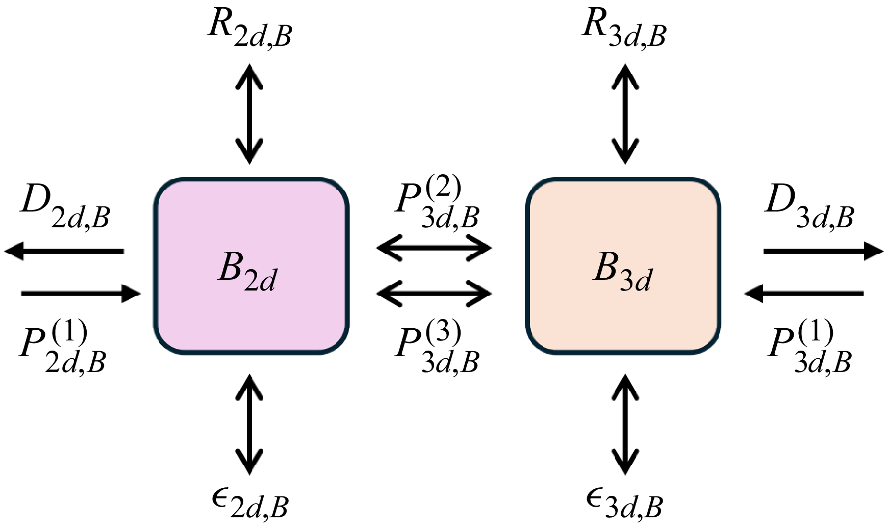
 B2d,B3d>0

 K2d
 K3d
 t2d
 t3d

 z
 t
 K1d
 K2d
 K2d,u
 K2d,w
 K3d
 K3d,u
 K3d,v
 K3d,w

 ∂tK1d
 ∂tK2d,u
 ∂tK2d,w
 ∂tK3,u
 ∂tK3d,v
 ∂tK3d,w

 B2d
 z
 t
 P2d,B(1)
 R2d,B
 −D2d,B

 B3d
 z
 t
 P3d,B(1)
 P3d,B(2)
 P3d,B(3)
 R3d,B
 −D3d,B
 −ϵ3d,B

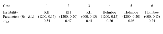
 Edg
 Kw

 E


 Pst=P1d↔2d,u+P1d↔3d,u
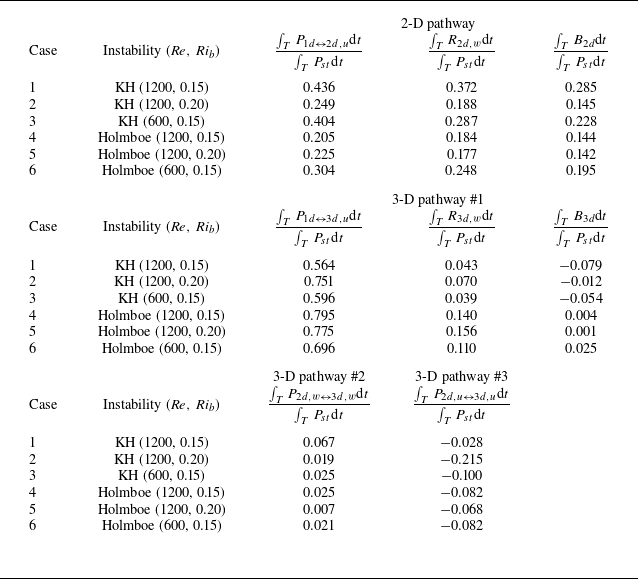
 T
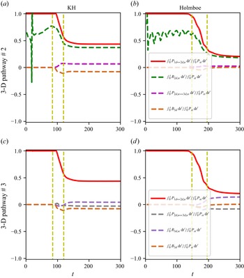
 Pst=P1d↔2d,u+P1d↔3d,u

 t={65,90,150}
 Ly=9
 Ly=18

 Ly=9
 Ly=18
 K2d
 K3d
 t2d
 t3d

 ku
 (∫0tP1d↔2d,udt′)
 ku
 (∫0tP1d↔3d,udt′)
 Ly=9
 Ly=18
 K2d
 K3d
 t2d
 t3d

 Open access

