1. Introduction
The Helmholtz decomposition
 $$\begin{eqnarray}\boldsymbol{u}=\boldsymbol{u}_{r}+\boldsymbol{u}_{d}=-\boldsymbol{{\rm\nabla}}\times (\boldsymbol{e}_{z}{\it\Psi})+\boldsymbol{{\rm\nabla}}{\it\phi}\end{eqnarray}$$
of the horizontal velocity,
 $\boldsymbol{u}$
, into a rotational and a divergent component is of great utility in geophysical fluid dynamics. Here,
 $\boldsymbol{{\rm\nabla}}$
is the horizontal gradient operator,
 $\boldsymbol{e}_{z}$
is the vertical unit vector,
 ${\it\Psi}$
is the stream function and
 ${\it\phi}$
is the velocity potential. The rotational component of the flow is mainly associated with geostrophically and hydrostatically balanced motions, while the divergent component is mainly associated with motions that are not balanced, such as gravity waves and stratified turbulence. The rotational component is dominant at planetary and synoptic scales (
 ${>}1000\ \text{km}$
) in the atmosphere. Analyses from general circulation models (GCMs) (Augier & Lindborg Reference Augier and Lindborg2013) show that the energy content in the rotational component is approximately 100 times larger than the energy content in the divergent component at these scales. However, at mesoscales (
 ${\sim}1{-}100\ \text{km}$
), where the energy spectra show a
 $k^{-5/3}$
-dependence (Nastrom & Gage Reference Nastrom and Gage1985) and the corresponding structure functions show an
 $r^{2/3}$
-dependence (Lindborg Reference Lindborg1999), simulations give quite divergent results. Here,
 $r$
is the separation distance and
 $k$
is the wave number. In a high-resolution GCM, Hamilton, Takahashi & Ohfuchi (Reference Hamilton, Takahashi and Ohfuchi2008) found that the rotational component was about four times larger than the divergent component at the mesoscales near the tropopause. Skamarock et al. (Reference Skamarock, Park, Klemp and Snyder2014) obtained rotational and divergent components of the same order at the mesoscales in the upper troposphere (8.5–10.5 km), while the divergent component was more than five times larger in the stratosphere (16–18 km). Waite & Snyder (Reference Waite and Snyder2013) and Waite & Snyder (Reference Waite and Snyder2014) argued that the transition from an approximate
 $k^{-3}$
-spectrum at synoptic scales to an approximate
 $k^{-5/3}$
-spectrum at mesoscales can be explained by the fact that a shallow
 $k^{-5/3}$
divergent spectrum crosses a steep
 $k^{-3}$
rotational spectrum. According to these authors the shallow divergent spectrum is a signature of gravity waves cascading downscale in accordance with the theory of Bartello (Reference Bartello1995). Results from simulations of moist baroclinic waves (Waite & Snyder Reference Waite and Snyder2013) as well as a dry mechanistic GCM (Brune & Becker Reference Brune and Becker2013) were used to support the hypothesis that the
 $k^{-5/3}$
mesoscale spectrum is a signature of gravity waves.
In order to analyse the problem from an experimental point of view it would be valuable to design a method by which it is possible to decompose the two-point velocity correlation
 $R(r)=\langle \boldsymbol{u}\boldsymbol{\cdot }\boldsymbol{u}^{\prime }\rangle$
, or the one-dimensional energy spectrum,
 $E(k)=\widehat{R}/2$
, into a rotational and a divergent part, with observational data as input. Here,
 $\langle \,\rangle$
is a mean value,
 $\boldsymbol{u}^{\prime }$
is the horizontal velocity measured at a point that is separated by a distance
 $r$
from the point where
 $\boldsymbol{u}$
is measured and
 $\widehat{\;}$
is the one-dimensional Fourier transform. A third alternative, which perhaps is the most attractive, would be to make a similar decomposition of the structure function,
 $D=\langle {\it\delta}\boldsymbol{u}\boldsymbol{\cdot }{\it\delta}\boldsymbol{u}\rangle$
, where
 ${\it\delta}\boldsymbol{u}=\boldsymbol{u}^{\prime }-\boldsymbol{u}$
. In measuring correlation functions, structure functions or energy spectra, it is customary to measure the longitudinal and transverse velocity components,
 $u_{l}$
and
 $u_{t}$
, separately, where
 $u_{l}$
is the component in the direction of the separation vector
 $\boldsymbol{r}$
between the two points and
 $u_{t}$
is a component that is perpendicular to
 $\boldsymbol{r}$
. From observations it is therefore possible to decompose these functions into a longitudinal and a transverse part. In the statistically homogenous case it is also possible to uniquely and exactly decompose them into a rotational and a divergent part. Thus, we can decompose these functions in two different ways:
 $$\begin{eqnarray}\displaystyle & R=R_{ll}+R_{tt}=R_{rr}+R_{dd}, & \displaystyle\end{eqnarray}$$
 $$\begin{eqnarray}\displaystyle & D=D_{ll}+D_{tt}=D_{rr}+D_{dd}, & \displaystyle\end{eqnarray}$$
 $$\begin{eqnarray}\displaystyle & E=E_{ll}+E_{tt}=E_{rr}+E_{dd}, & \displaystyle\end{eqnarray}$$
 $ll$
and
 $tt$
as subscripts are calculated from the longitudinal and transverse velocity components respectively, while the objects with
 $rr$
and
 $dd$
as subscripts are calculated from the rotational and divergent velocity components respectively. For example,
 $D_{rr}=\langle {\it\delta}\boldsymbol{u}_{r}\boldsymbol{\cdot }{\it\delta}\boldsymbol{u}_{r}\rangle$
. Our problem can now be formulated as follows: find a method to go from the longitudinal–transverse decomposition to the Helmholtz decomposition!
Two different approaches have been developed to solve this problem. Lindborg (Reference Lindborg2007) showed that the two-point correlation functions of vertical vorticity,
 $Q=\langle {\it\zeta}{\it\zeta}^{\prime }\rangle$
, and horizontal divergence,
 $P=\langle dd^{\prime }\rangle$
, where
 ${\it\zeta}={\rm\nabla}^{2}{\it\Psi}$
and
 $d={\rm\nabla}^{2}{\it\phi}$
, under the assumption of axisymmetry (often referred to as ‘horizontal isotropy’) are related to
 $R_{ll}$
and
 $R_{tt}$
as
 $$\begin{eqnarray}\displaystyle & \displaystyle Q=\frac{1}{r}\frac{\text{d}R_{ll}}{\text{d}r}-\frac{1}{r^{2}}\frac{\text{d}}{\text{d}r}\left(r^{2}\frac{\text{d}R_{tt}}{\text{d}r}\right), & \displaystyle\end{eqnarray}$$
 $$\begin{eqnarray}\displaystyle & \displaystyle P=\frac{1}{r}\frac{\text{d}R_{tt}}{\text{d}r}-\frac{1}{r^{2}}\frac{\text{d}}{\text{d}r}\left(r^{2}\frac{\text{d}R_{ll}}{\text{d}r}\right). & \displaystyle\end{eqnarray}$$
 $Q$
and
 $P$
are related to the corresponding transforms of
 $R_{rr}$
and
 $R_{dd}$
through the relations
 $\widetilde{Q}=k^{2}\widetilde{R}_{rr}$
and
 $\widetilde{P}=k^{2}\widetilde{R}_{dd}$
. The functions
 $R_{rr}$
and
 $R_{dd}$
can be retrieved from
 $\widetilde{R}_{rr}$
and
 $\widetilde{R}_{dd}$
, as can the one-dimensional spectra,
 $E_{rr}$
and
 $E_{dd}$
. However, the procedure is quite complicated and also involves second-order differentiation of observational data, which can lead to errors. The other approach was recently developed by Bühler, Callies & Ferrari (Reference Bühler, Callies and Ferrari2014) who constructed a method by which
 $E_{rr}$
and
 $E_{dd}$
can be retrieved from
 $E_{ll}$
and
 $E_{tt}$
by introducing two auxiliary spectral functions which they denoted by
 $D^{{\it\Psi}}$
and
 $D^{{\it\phi}}$
. To avoid confusing these functions with structure functions we will instead call them
 $S^{{\it\Psi}}$
and
 $S^{{\it\phi}}$
. Bühler et al. (Reference Bühler, Callies and Ferrari2014) derived the following set of equations:
 $$\begin{eqnarray}\displaystyle & \displaystyle E_{ll}(k)=S^{{\it\Psi}}(k)-k\frac{\text{d}}{\text{d}k}S^{{\it\phi}}(k), & \displaystyle\end{eqnarray}$$
 $$\begin{eqnarray}\displaystyle & \displaystyle E_{tt}(k)=S^{{\it\phi}}(k)-k\frac{\text{d}}{\text{d}k}S^{{\it\Psi}}(k), & \displaystyle\end{eqnarray}$$
 $$\begin{eqnarray}\displaystyle & \displaystyle E_{rr}(k)=S^{{\it\Psi}}(k)-k\frac{\text{d}}{\text{d}k}S^{{\it\Psi}}(k), & \displaystyle\end{eqnarray}$$
 $$\begin{eqnarray}\displaystyle & \displaystyle E_{dd}(k)=S^{{\it\phi}}(k)-k\frac{\text{d}}{\text{d}k}S^{{\it\phi}}(k). & \displaystyle\end{eqnarray}$$
 $E_{ll}$
and
 $E_{tt}$
, Bühler et al. inverted (1.7) and (1.8) to obtain
 $S^{{\it\Psi}}$
and
 $S^{{\it\phi}}$
, which they used in (1.9) and (1.10) to finally calculate
 $E_{rr}$
and
 $E_{dd}$
, a procedure involving interpolation of
 $E_{ll}$
and
 $E_{tt}$
to a logarithmic grid as well as numerical differentiation.
In this paper, we will show that there is, in fact, an amazingly simple solution to the problem of making a Helmholtz decomposition from observational longitudinal and transverse correlation functions, structure functions or spectra. We will also apply this solution to structure functions calculated by Cho & Lindborg (Reference Cho and Lindborg2001) from aircraft data.
2. Solution
A simple solution to the problem we have formulated in the introduction can be found by noting that the following relations hold:
 $$\begin{eqnarray}\displaystyle & Q=-{\rm\nabla}^{2}R_{rr}, & \displaystyle\end{eqnarray}$$
 $$\begin{eqnarray}\displaystyle & P=-{\rm\nabla}^{2}R_{dd}. & \displaystyle\end{eqnarray}$$
 $$\begin{eqnarray}\displaystyle & \displaystyle -\frac{\text{d}}{\text{d}r}\left(r\frac{\text{d}R_{rr}}{\text{d}r}\right)=\frac{\text{d}R_{ll}}{\text{d}r}-\frac{1}{r}\frac{\text{d}}{\text{d}r}\left(r^{2}\frac{\text{d}R_{tt}}{\text{d}r}\right), & \displaystyle\end{eqnarray}$$
 $$\begin{eqnarray}\displaystyle & \displaystyle -\frac{\text{d}}{\text{d}r}\left(r\frac{\text{d}R_{dd}}{\text{d}r}\right)=\frac{\text{d}R_{tt}}{\text{d}r}-\frac{1}{r}\frac{\text{d}}{\text{d}r}\left(r^{2}\frac{\text{d}R_{ll}}{\text{d}r}\right). & \displaystyle\end{eqnarray}$$
 $r\rightarrow \infty$
, these equations can be integrated to give
 $$\begin{eqnarray}\displaystyle & \displaystyle R_{rr}=R_{tt}-\int _{r}^{\infty }\frac{1}{r}(R_{tt}-R_{ll})\text{d}r, & \displaystyle\end{eqnarray}$$
 $$\begin{eqnarray}\displaystyle & \displaystyle R_{dd}=R_{ll}+\int _{r}^{\infty }\frac{1}{r}(R_{tt}-R_{ll})\text{d}r. & \displaystyle\end{eqnarray}$$
 $(R_{tt}-R_{ll})\sim r^{2}$
as
 $r\rightarrow 0$
, which shows the convergence of the integral in this limit. The structure functions satisfy the same equations (2.3) and (2.4) as the corresponding correlation functions. However, to solve the equations in this case we have to use the fact that these functions go to zero as
 $r\rightarrow 0$
. The solutions for the structure functions are
 $$\begin{eqnarray}\displaystyle & \displaystyle D_{rr}=D_{tt}+\int _{0}^{r}\frac{1}{r}(D_{tt}-D_{ll})\text{d}r, & \displaystyle\end{eqnarray}$$
 $$\begin{eqnarray}\displaystyle & \displaystyle D_{dd}=D_{ll}-\int _{0}^{r}\frac{1}{r}(D_{tt}-D_{ll})\text{d}r. & \displaystyle\end{eqnarray}$$
 $(D_{tt}-D_{ll})\rightarrow 0$
as
 $r\rightarrow \infty$
, which shows the convergence of the integral in this limit. Using (2.3) and (2.4) and the fact that the spectral functions are the Fourier transforms of the correlation functions it is straightforward to derive the following equations for the spectral functions:
 $$\begin{eqnarray}\displaystyle & \displaystyle \frac{\text{d}}{\text{d}k}(kE_{rr})=k\frac{\text{d}E_{tt}}{\text{d}k}+E_{ll}, & \displaystyle\end{eqnarray}$$
 $$\begin{eqnarray}\displaystyle & \displaystyle \frac{\text{d}}{\text{d}k}(kE_{dd})=k\frac{\text{d}E_{ll}}{\text{d}k}+E_{tt}, & \displaystyle\end{eqnarray}$$
 $$\begin{eqnarray}\displaystyle & \displaystyle E_{rr}=E_{tt}+\frac{1}{k}\int _{k}^{\infty }(E_{tt}-E_{ll})\text{d}k, & \displaystyle\end{eqnarray}$$
 $$\begin{eqnarray}\displaystyle & \displaystyle E_{dd}=E_{ll}-\frac{1}{k}\int _{k}^{\infty }(E_{tt}-E_{ll})\text{d}k. & \displaystyle\end{eqnarray}$$
3. Application to aircraft data
Cho & Lindborg (Reference Cho and Lindborg2001) calculated
 $D_{ll}$
and
 $D_{tt}$
using data from 7630 commercial flights collected in the MOZAIC data set (Marenco et al.
Reference Marenco, Thouret, Nédeléc, Smit, Helten, Kley, Karcher, Simon, Law, Pyle, Poschmann, Wrede, Von Hume and Cook1998) between August 1994 and December 1997. Fortunately, the calculated structure functions were saved by John Cho who provided the author with a number of data files containing the results. Equations (2.7) and (2.8) could thus be used to calculate
 $D_{rr}$
and
 $D_{dd}$
from
 $D_{ll}$
and
 $D_{tt}$
, where the integration was performed directly on the calculated points using the trapezoidal rule. Cho & Lindborg (Reference Cho and Lindborg2001) divided the data into two altitude bands, the upper troposphere and the lower stratosphere. The ozone concentration was used to differentiate between the troposphere and the stratosphere. If the ozone concentration was over 200 ppbv for both of the points in each pair the result was classified as stratospheric and if the concentration was under 200 ppbv for both points the result was classified as tropospheric. If one of the points had an ozone concentration under the threshold and the other point had one over the threshold this pair of points was not used in the analysis. The structure functions were calculated for 140 separation distances between 2 and 2510 km, with separation distance intervals of 2 km in
 $[2,50]\ \text{km}$
, 4 km in
 $[50,150]\ \text{km}$
, 8 km in
 $[150,350]\ \text{km}$
, 16 km in
 $[350,750]\ \text{km}$
, 32 km in
 $[750,1550]\ \text{km}$
and 64 km in
 $[1550,2510]\ \text{km}$
. For other details regarding the computational procedure the reader is referred to Cho & Lindborg (Reference Cho and Lindborg2001).
In order to use (2.7) and (2.8) we first have to decide how to treat the integration in the missing interval
 $r<r_{min}=2\ \text{km}$
. The simplest method would be to set this contribution to the integral to zero. Another method is to use the data points in
 $[2,20]\ \text{km}$
to make a curve fit,
 $D_{ll}=a_{1}r^{2/3}$
and
 $D_{tt}=a_{2}r^{2/3}$
, assume that
 $D_{ll}$
and
 $D_{tt}$
also have this functional dependence for
 $r<r_{min}$
and calculate the integral over the missing interval as
 $$\begin{eqnarray}\displaystyle \int _{0}^{r_{min}}\frac{1}{r}(D_{tt}-D_{ll})\text{d}r=\frac{3}{2}(a_{2}-a_{1})r_{min}^{2/3}. & & \displaystyle\end{eqnarray}$$
We use this method. However, since it turns out that
 $a_{2}\approx a_{1}$
, for both the stratospheric and the tropospheric data, the two methods give very similar results.
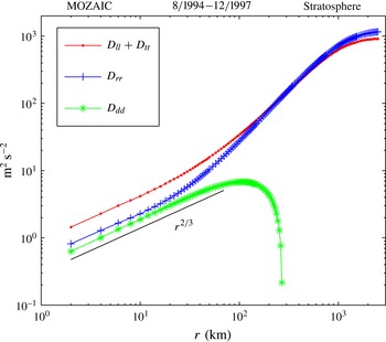
In figure 1,
 $D_{rr}$
,
 $D_{dd}$
and
 $D_{ll}+D_{tt}$
calculated from the lower stratospheric data are plotted. Both
 $D_{rr}$
and
 $D_{dd}$
show a nice
 $r^{2/3}$
-dependence in the interval
 $r\in [2,20]\ \text{km}$
. In this interval
 $D_{rr}/D_{dd}\approx 1.2$
. For gravity waves all kinetic energy is in the divergent component. For inertia–gravity waves the ratio between rotational and divergent energy is equal to
 $f^{2}/{\it\omega}^{2}<1$
, where
 ${\it\omega}$
is the frequency and
 $f$
is the Coriolis parameter. Any realistic frequency distribution would give a ratio
 $D_{rr}/D_{dd}$
substantially smaller than unity, while we find that this ratio is, in fact, somewhat larger than unity. Thus, gravity waves and inertia–gravity waves can be excluded as the principal dynamic agent behind the observed structure functions. On the other hand, the result is consistent with stratified turbulence, with a downscale energy cascade of Kolmogorov type and approximate equipartition between rotational and divergent energy (Lindborg & Brethouwer Reference Lindborg and Brethouwer2007). For
 $r>20\ \text{km}$
,
 $D_{rr}$
starts to grow faster than
 $r^{2/3}$
, while
 $D_{dd}$
starts to grow slightly more slowly and reaches a maximum at
 $r\approx 100\ \text{km}$
, from where it drops to below zero at
 $r\approx 300\ \text{km}$
(not shown in the figure), which is clearly unphysical, since
 $D_{dd}$
is by definition positive definite. At
 $r\sim 1000\ \text{km}$
we see that
 $D_{rr}>D_{ll}+D_{tt}$
, which is also unphysical, for the same reason. We will discuss the reason behind these unphysical results after presenting the results for the upper troposphere.
Decomposition of
 $D_{ll}+D_{tt}$
into
 $D_{rr}$
and
 $D_{dd}$
in the lower stratosphere.

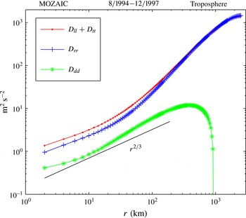
In figure 2,
 $D_{rr}$
,
 $D_{dd}$
and
 $D_{ll}+D_{tt}$
calculated from the upper tropospheric data are plotted. No clean
 $r^{2/3}$
-dependence is visible for any of the curves. At kilometre scales, the slope is somewhat smaller than
 $2/3$
, and at larger scales it becomes larger for all curves. However, the overall slope of
 $D_{dd}$
in the range
 $[2,400]\ \text{km}$
is quite close to
 $2/3$
. In the range
 $[2,100]\ \text{km}$
we find that
 $D_{rr}/D_{dd}\approx 3$
, a fact that is again pointing against the gravity wave hypothesis. The fact that no clean
 $r^{2/3}$
-range is observed indicates that there is no clean cascade range in the upper troposphere. It can be speculated that the reason for this is that there is a non-negligible local forcing by release of latent heat at mesoscales in the upper troposphere (Waite & Snyder Reference Waite and Snyder2013), which causes the structure functions to deviate from the ideal
 $r^{2/3}$
-dependence.
Decomposition of
 $D_{ll}+D_{tt}$
into
 $D_{rr}$
and
 $D_{dd}$
in the upper troposphere.

There is another interesting difference between the stratospheric and tropospheric results, and that is the separation distance at which
 $D_{dd}$
becomes negative, which is the same separation distance as that at which
 $D_{rr}$
exceeds
 $D_{ll}+D_{tt}$
. As already pointed out, this is clearly unphysical. In the stratosphere this happens already at
 $r\approx 300\ \text{km}$
, while in the troposphere it happens at
 $r\approx 1000\ \text{km}$
. There can be no doubt that the reason why we obtain this unphysical result is that the assumption of axisymmetry or ‘horizontal isotropy’ is not perfectly fulfilled at large scales. In dealing with a data set containing a huge amount of data from flights going in different directions all over the globe this assumption may not necessarily be interpreted as a dynamic assumption, but rather an assumption saying that any dynamic anisotropy that may be present in the data will be smeared out when we average over so many flights going in different directions at different locations. As we pointed out in the introduction, rotational kinetic energy is about one hundred times larger than divergent kinetic energy at 1000 km scales in GCMs. We would thus expect to see that
 $D_{rr}$
should be smaller than
 $D_{ll}+D_{tt}$
by one or a few per cent at these scales. In the troposphere, it is difficult to distinguish
 $D_{rr}$
from
 $D_{ll}+D_{tt}$
with the eye at these scales, as seen in figure 2. At
 $r=1000\ \text{km}$
the two curves are almost equal, and at the largest separation distance,
 $r=2510\ \text{km}$
,
 $D_{rr}$
exceeds
 $D_{ll}+D_{dd}$
by 2 %. We can thus conclude that we have managed to determine
 $D_{rr}$
with a relative error of a few per cent, at these scales. It thus appears that it is to this degree that the assumption of axisymmetry is fulfilled for the tropospheric data at synoptic scales. Indeed, this is quite a remarkably high degree of accuracy. For the stratospheric data, the accuracy is less impressive. At
 $r=1000\ \text{km}\ D_{rr}$
exceeds
 $D_{ll}+D_{tt}$
by 16 %, while we expect that it should be one or a few per cent smaller. Therefore, the relative error of
 $D_{rr}$
is approximately 20 % at 1000 km scales. Thus, the assumption of axisymmetry seems to be quite well fulfilled for the tropospheric data, while it is less well fulfilled for the stratospheric data. It is difficult to know the reason for this difference, but it may be that the stratospheric flight tracks are more systematically aligned with the jet streams than the tropospheric tracks.
The absolute error of
 $D_{dd}$
, due to lack of axisymmetry, is equal to minus the absolute error of
 $D_{rr}$
, since the two errors must cancel each other. Since we expect that
 $D_{dd}$
should be of the order of one per cent of
 $D_{rr}$
at 1000 km scales, the relative error of
 $D_{dd}$
is more than 100 % at these scales. At scales of the order of 10 km the situation is very different. Here,
 $D_{dd}$
is of the same order of magnitude as
 $D_{rr}$
and the relative errors are therefore of the same order. There is strong reason to believe that axisymmetry is much better fulfilled at
 $r\sim 10\ \text{km}$
than at
 $r\sim 1000\ \text{km}$
, not only because the data have been averaged over many flight directions at different locations, but because axisymmetry in a dynamic sense is satisfied at these scales. In other words, at these scales the statistics can be assumed to be genuinely independent of direction. Based on observations of the two-dimensional spherical harmonic spectrum calculated from a GCM, Hamilton et al. (Reference Hamilton, Takahashi and Ohfuchi2008) argued that axisymmetry is fairly well fulfilled at scales smaller than 400 km, while it is fulfilled to a lesser degree at planetary and synoptic scales. Of course, this is exactly what is expected on intuitive grounds. Large-scale structures such as jets have a clear directional preference, while small-scale structures have no such preference, at least not to the same extent as large-scale structures. If we only make the modest assumption that axisymmetry is as well fulfilled at 10 km scales as it is at 1000 km scales, we still obtain a relative error that is not larger than a few per cent in the troposphere and 20 % in the stratosphere. The conclusion that gravity waves cannot be the principal explanation of the observed structure functions at 10 km scales is therefore valid.
4. Conclusions
We have derived expressions by which the rotational and divergent correlation functions, spectra and structure functions can be calculated from the corresponding longitudinal and transverse functions. The expressions are far simpler than the expressions derived in previous analyses (Lindborg Reference Lindborg2007; Bühler et al.
Reference Bühler, Callies and Ferrari2014). The decomposition can be made by directly integrating observational functions using a simple trapezoidal rule. We have applied the derived formulae to the structure functions calculated by Cho & Lindborg (Reference Cho and Lindborg2001) from the MOZAIC data set. In the lower stratosphere we found a clean
 $r^{2/3}$
-dependence of both
 $D_{rr}$
and
 $D_{dd}$
for
 $r\in [2,20]\ \text{km}$
, with
 $D_{rr}/D_{dd}\approx 1.2$
. This is consistent with stratified turbulence (Lindborg Reference Lindborg2006) with a downscale energy cascade of Kolmogorov type and approximate equipartition between divergent and rotational energy, but not with the gravity wave hypothesis. In the upper troposphere we found no clean
 $r^{2/3}$
-range and
 $D_{rr}/D_{dd}\approx 3$
in the range
 $[2,100]\ \text{km}$
. Given these two observations it seems difficult to interpret the upper tropospheric data as evidence of stratified turbulence in a clean sense. However, the overall slope of
 $D_{dd}$
for
 $r\in [2,400]\ \text{km}$
is quite close to
 $2/3$
. The fact that no clean
 $r^{2/3}$
-range is observed may be explained as a result of direct forcing by release of latent heat (Waite & Snyder Reference Waite and Snyder2013) at the mesoscales. The results are generally consistent with the previous results of Lindborg (Reference Lindborg2007), who found that the ratio between rotational and divergent energy was close to two, when an average was made over both tropospheric and stratospheric data. They are also consistent with the results of Cho & Newell (Reference Cho and Newell1999), who measured the ratio
 $E_{ll}/E_{tt}$
using aircraft data over the Pacific Ocean at altitudes between 2 and 12 km. An average over these altitudes and latitudes larger than
 $15^{\circ }$
gave
 $E_{ll}/E_{tt}\approx 0.8$
. With a
 $k^{-5/3}$
spectral dependence, which was also measured by Cho & Newell (Reference Cho and Newell1999), this gives
 $E_{rr}/E_{dd}\approx 2.6$
, which is very close to the corresponding ratio we have calculated in the troposphere in this study.
As for a comparison with results from GCMs, it may be pointed out that in most such studies the ratio
 $E_{rr}/E_{dd}$
is found to be smaller in the stratosphere than in the troposphere, which is consistent with the results from this analysis. However, in several studies (e.g. Skamarock et al.
Reference Skamarock, Park, Klemp and Snyder2014) the divergent component is very dominant in the stratosphere, which is not consistent with what we have found here. It seems that Hamilton et al. (Reference Hamilton, Takahashi and Ohfuchi2008) is the study that is coming closest to the results we have obtained in the present study.
Lilly (Reference Lilly1983) developed the hypothesis that there is an upscale or inverse energy cascade through the atmospheric mesoscales. This hypothesis was recently revived by Cencini, Muratori-Ginanneschi & Vulpiani (Reference Cencini, Muratori-Ginanneschi and Vulpiani2011) and Xia et al. (Reference Xia, Byrne, Falkovich and Shats2011). Based on measurements of third-order structure functions in the lower stratosphere, Cho & Lindborg (Reference Cho and Lindborg2001) concluded that there is a downscale energy cascade through the mesoscales, a conclusion that was reinforced by comparing the observed third-order structure functions with corresponding functions from numerical simulations (Deusebio, Augier & Lindborg Reference Deusebio, Augier and Lindborg2014). On analysing data from a high-resolution GCM, Augier & Lindborg (Reference Augier and Lindborg2013) also found clear evidence of a downscale energy cascade. The present study gives additional evidence pointing against the inverse cascade hypothesis. An inverse cascade emerges in flows having a second conserved quadratic quantity in addition to energy. In two-dimensional turbulence this second quadratic quantity is enstrophy, which is half the square of the vorticity, and in quasi-geostrophic turbulence (Charney Reference Charney1971) it is potential enstrophy, which is half the square of the Charney potential vorticity. Here, we have found that the divergent energy is of the same order of magnitude as the rotational energy at the mesoscales, and for this reason there can be no second conserved quadratic quantity, which is quite easy to show. Consequently, there is no reason to believe that there should be an inverse energy cascade.
The analysis we have carried out has several advantages compared with the analysis carried out by Lindborg (Reference Lindborg2007). First, in contrast to Lindborg (Reference Lindborg2007) we have here made a discrimination between upper tropospheric and lower stratospheric data, which showed that there are some clear differences between the lower stratosphere and the upper troposphere. Second, the accuracy of the method permitted us to work directly on the calculated structure functions, rather than on curve fits, as were used by Lindborg (Reference Lindborg2007). Finally, the new formulae permit us to investigate the limitations of the assumption of axisymmetry at large scales. At synoptic scales it can be expected that
 $D_{rr}$
should be smaller than
 $D_{ll}+D_{tt}$
by a few per cent. Instead, we found that it was a few per cent larger for the tropospheric data and 16 % larger for the stratospheric data. This clearly unphysical result must be due to the fact that the assumption of axisymmetry is not fulfilled at these scales. The extent to which
 $D_{rr}$
exceeds
 $D_{ll}+D_{tt}$
at these scales also provides us with a measure of the relative error at these scales. If it is assumed that the relative error is not larger at smaller scales, then there can be no large error in the estimate of the ratio
 $D_{rr}/D_{dd}$
.
We hope that this paper will stimulate further discussions on the mesoscale dynamics in the atmosphere.
Acknowledgements
The author would like to thank J. Cho who provided the files containing the structure functions that we calculated from the MOZAIC data set thirteen years ago. O. Bühler, J. Callies, and R. Ferrari are thanked for sharing and discussing their work in Bühler et al. (Reference Bühler, Callies and Ferrari2014) prior to its publication.
Appendix A. Proof of relations (2.1) and (2.2)
We prove the relations (2.1) and (2.2) using the assumption of statistical homogeneity. Let
 $\boldsymbol{{\rm\nabla}}_{x}=\boldsymbol{e}_{x}\partial _{x}+\boldsymbol{e}_{y}\partial _{y}$
be the horizontal gradient operator acting on quantities measured at a point
 $\boldsymbol{x}$
,
 $\boldsymbol{{\rm\nabla}}_{x^{\prime }}$
the corresponding operator acting on quantities measured at a point
 $\boldsymbol{x}^{\prime }$
and
 $\boldsymbol{r}=\boldsymbol{x}^{\prime }-\boldsymbol{x}$
. Then we have
 $$\begin{eqnarray}\displaystyle P=\langle {\rm\nabla}_{x}^{2}{\it\phi}{\rm\nabla}_{x^{\prime }}^{2}{\it\phi}^{\prime }\rangle ={\rm\nabla}_{x}^{2}{\rm\nabla}_{x^{\prime }}^{2}\langle {\it\phi}{\it\phi}^{\prime }\rangle ={\rm\nabla}_{r}^{4}\langle {\it\phi}{\it\phi}^{\prime }\rangle , & & \displaystyle\end{eqnarray}$$
where
 $\boldsymbol{{\rm\nabla}}_{r}$
is the horizontal gradient operator with respect to the separation vector
 $\boldsymbol{r}$
. In the first step we have used the fact that
 $\boldsymbol{x}$
and
 $\boldsymbol{x}^{\prime }$
can be treated as independent variables. In the second step we have made the variable transformation
 $$\begin{eqnarray}\displaystyle & \boldsymbol{r}=\boldsymbol{x}^{\prime }-\boldsymbol{x}, & \displaystyle\end{eqnarray}$$
 $$\begin{eqnarray}\displaystyle & {\bf\xi}=\boldsymbol{x}^{\prime }, & \displaystyle\end{eqnarray}$$
 $\boldsymbol{{\rm\nabla}}_{x}\curvearrowright -\boldsymbol{{\rm\nabla}}_{r}$
and
 $\boldsymbol{{\rm\nabla}}_{x^{\prime }}\curvearrowright \boldsymbol{{\rm\nabla}}_{r}+\boldsymbol{{\rm\nabla}}_{{\it\xi}}$
. Then we have used that the correlation function is independent of
 ${\bf\xi}$
, by statistical homogeneity. In a similar way we find
 $$\begin{eqnarray}\displaystyle R_{dd}=\langle \boldsymbol{{\rm\nabla}}_{x}{\it\phi}\boldsymbol{\cdot }\boldsymbol{{\rm\nabla}}_{x^{\prime }}{\it\phi}^{\prime }\rangle =\boldsymbol{{\rm\nabla}}_{x}\boldsymbol{\cdot }\boldsymbol{{\rm\nabla}}_{x^{\prime }}\langle {\it\phi}{\it\phi}^{\prime }\rangle =-{\rm\nabla}_{r}^{2}\langle {\it\phi}{\it\phi}^{\prime }\rangle . & & \displaystyle\end{eqnarray}$$
Combining (A 1) and (A 4), we obtain (2.2). Using the same technique we find
 $$\begin{eqnarray}\displaystyle & Q=\langle \boldsymbol{{\rm\nabla}}_{x}\times (\boldsymbol{{\rm\nabla}}_{x}\times ({\it\Psi}\boldsymbol{e}_{z}))\boldsymbol{\cdot }\boldsymbol{{\rm\nabla}}_{x^{\prime }}\times (\boldsymbol{{\rm\nabla}}_{x^{\prime }}\times ({\it\Psi}^{\prime }\boldsymbol{e}_{z}))\rangle =\langle {\rm\nabla}_{x}^{2}{\it\Psi}{\rm\nabla}_{x^{\prime }}^{2}{\it\Psi}^{\prime }\rangle ={\rm\nabla}_{r}^{4}\langle {\it\Psi}{\it\Psi}^{\prime }\rangle , & \displaystyle\end{eqnarray}$$
 $$\begin{eqnarray}\displaystyle & R_{rr}=\langle \boldsymbol{{\rm\nabla}}_{x}\times ({\it\Psi}\boldsymbol{e}_{z})\boldsymbol{\cdot }\boldsymbol{{\rm\nabla}}_{x^{\prime }}\times ({\it\Psi}^{\prime }\boldsymbol{e}_{z})\rangle =\langle \boldsymbol{{\rm\nabla}}_{x}{\it\Psi}\boldsymbol{\cdot }\boldsymbol{{\rm\nabla}}_{x^{\prime }}{\it\Psi}^{\prime }\rangle =-{\rm\nabla}_{r}^{2}\langle {\it\Psi}{\it\Psi}^{\prime }\rangle . & \displaystyle\end{eqnarray}$$