
1 Introduction
Vortex pairs have been an area of significant interest as a result of their importance in both the study of fundamental fluid mechanics and applied engineering. With modern advances in numerical and experimental methods uncovering the significance of coherent structures in turbulent flows (Hussain Reference Hussain1986; Fiedler Reference Fiedler1988), the dynamics and stability of vortex interaction are evidently integral to not only large-scale vortex systems, but to all flow scales down to the mechanisms governing development of micro-scale turbulence. In particular, parallel vortex pairs provide an elementary vortex interaction configuration further motivated by their relevance to aircraft wakes.
The far field wake behind a lifting wing is characterised by the persistence of two strong trailing counter-rotating vortices after the initial roll-up of the near wake (for details, see Spalart (Reference Spalart1998)). These counter-rotating vortex pairs control the motion of exhaust gases at cruise conditions (Gerz & Ehret Reference Gerz and Ehret1997) and pose a significant hazard to other aircraft at take-off and landing due to the induced rolling moment. As the persistence of trailing vortices behind large aircraft may constitute a hazard to following aircraft, an understanding of the dynamics and instabilities of this configuration of vortices is critically important to safety (Rossow Reference Rossow1999; Gerz, Holzäpfel & Darracq Reference Gerz, Holzäpfel and Darracq2002). Specifically, the interaction between a vortex pair and a ground plane occurs during the approach and landing of aircraft, for which the finite-wing vortices interact with the runway. This considerable practical interest provides the underlying reason for the large volume of literature on attempting to understand and ultimately accelerate the decay of the wake.
Equally strong ( $\unicode[STIX]{x1D6E4}=\unicode[STIX]{x1D6E4}_{1}=-\unicode[STIX]{x1D6E4}_{2}$, where
 $\unicode[STIX]{x1D6E4}$ is the circulation) counter-rotating vortex pairs, separated by distance
 $b$, translate with a constant velocity value of
 $(\unicode[STIX]{x1D6E4}/2\unicode[STIX]{x03C0}b)$ normal to the plane on which they lie (Lamb Reference Lamb1932) and undergo two primary three-dimensional instabilities. The instabilities may be characterised by their respective wavelengths. The growth of both the long- and short-wavelength instabilities can be induced in a single stable vortex by the imposition of an external strain field (Moore & Saffman Reference Moore and Saffman1971). The presence of the parallel vortex induces such a field, enabling the cooperative growth of the instabilities to develop in both vortices (Leweke & Williamson Reference Leweke and Williamson1998).
The long-wavelength instability involves sinusoidally radial displacement of vortices without influence on their core structure. It can be observed behind aircraft where the wake vortices are visualised by condensation (Jacob Reference Jacob1995), resulting in long axially sinusoidal wavelengths relative to the initial vortex separation distance. Crow (Reference Crow1970), who undertook the first theoretical study of this instability, showed that counter-rotating vortex pairs mutually interact, leading to the amplification of low wavenumber perturbations and resulting in the deformation of the vortex pair into axially periodic long-wavelength structures. By using a vortex filament model, Crow found that the instability mode is symmetric and sinusoidal, and initially confined to planes inclined at close to  $45^{\circ }$ to the plane on which both vortices initially lie. The dynamics of this eponymous ‘Crow’ instability arises from a balancing of three plane rotation mechanisms resulting in radial stretching of the perturbation. Kelvin (Reference Kelvin1880) illustrated the self-induced rotation of the instability plane of a single sinusoidally perturbed vortex. The introduction of the second vortex mutually induces counter-rotation and radial stretching on the plane where the perturbation grows. When the plane rotation effects cancel, the wave is held at a constant angle with a positive component of radial strain, leading to exponential growth in amplitude. To tackle the issue of the singularity of the vortex filament model, Crow introduced a ‘cutoff’ technique, which involves integrating the Biot–Savart law for the self-induced motion of the vortex filament up to a finite region near the vortex core. The choice of the cutoff distance was based on solutions by Thompson (Reference Thompson1910) for both a vortex ring and rotating sinusoid with constant vorticity in the core. Bliss (Reference Bliss1970) and Widnall, Bliss & Zalay (Reference Widnall, Bliss and Zalay1971) extended the stability analysis by asymptotic matching of the inner (close to the vortex core) solution of the vorticity conservation equation and the outer filament based Biot–Savart law. This allowed for general vortex velocity profiles with axial flow to be considered, and an analytical expression for the appropriate cutoff distance to be used in Crow’s approach was derived. This expression was based on a Batchelor vortex of radius
 $a$ and axial flow parameter
 $W$. The effects of vorticity distributions on the stability of vortex pairs was further studied by Moore & Saffman (Reference Moore and Saffman1973) and Klein, Majda & Damodaran (Reference Klein, Majda and Damodaran1995).
The evolution of the Crow instability in parallel counter-rotating vortex pairs first results in the distortion of the initial sinusoidal deformation at large instability amplitudes and results in the periodic connection of the cores, eventually breaking down into a series of periodic vortex rings (Scorer & Davenport Reference Scorer and Davenport1970; Garten et al. Reference Garten, Werne, Fritts and Arendt2001). As the elliptic rings descend in the fluid, the major and minor axes of the ellipse switch, and the vortices reconnect for a second time, as shown experimentally by Leweke & Williamson (Reference Leweke and Williamson2011). Moore & Saffman (Reference Moore and Saffman1972) integrated the nonlinear system until the vortex pair was almost touching and found that the instability continues to grow to large amplitudes in close agreement with the linear theory. Crouch (Reference Crouch1997) and Fabre, Jacquin & Loof (Reference Fabre, Jacquin and Loof2002) applied and extended the model to multiple vortices, and studied the aircraft wake model composed of both the outer wing-tip vortex pair and an inner vortex pair rotating in the opposite direction, generated from the flaps or a horizontal tail. Optimal forcing of the Crow mode for accelerating the growth rate has been studied theoretically by Brion, Sipp & Jacquin (Reference Brion, Sipp and Jacquin2007), with further numerical studies (Johnson, Brion & Jacquin Reference Johnson, Brion and Jacquin2016) finding the growth rate increasing approximately twofold with optimal linear forcing. Crouch (Reference Crouch2005) found practical methods of both active and passive control for accelerating the long-wave instability.
The elliptic instability is characterised by short-wavelength perturbations which develop inside and modify the internal structure of the vortex cores. As the axial wavelength of the instability is of the same order as the core size of the vortices, the vortex filament approach is incapable of capturing the physics of this mode. Visualisations of these instabilities (Leweke & Williamson Reference Leweke and Williamson1998) were compared to the theoretical elliptic instability (Moore & Saffman Reference Moore and Saffman1975; Tsai & Widnall Reference Tsai and Widnall1976) of a vortex ring, providing the analytical framework for the instability mode. It was found that the elliptic instability results from interaction between the perturbation waves (Kelvin modes) and strain modification of the base flow due to the strain field of the other vortex (Roy et al. Reference Roy, Leweke, Thompson and Hourigan2011). The external strain produces flow with elliptical streamlines in the vortex core, which is unstable to three-dimensional perturbations. The instability is present in a number of flow configurations reviewed by Kerswell (Reference Kerswell2002). Lacaze, Ryan & Le Dizàs (Reference Lacaze, Ryan and Le Dizàs2007) and Fabre, Sipp & Jacquin (Reference Fabre, Sipp and Jacquin2006) determined the linear modes of Lamb–Oseen vortices following the work of Kelvin (Reference Kelvin1880) on linear modes of Rankine vortices. The elliptic instability is expected to influence the dynamics of multiple vortices generated by aircraft wings. Leweke & Williamson (Reference Leweke and Williamson1998) showed that the addition of the short-wave perturbations to the Crow instability increased the growth rate by  ${\sim}20\,\%$. Furthermore, it was shown that the elliptic instability breaks the symmetry of the long-wave mode, and the presence of both modes results in the development of a series of secondary vortex pairs during the nonlinear growth phase.
The presence of a ground plane in the vicinity of the vortex pair substantially alters the dynamics and stability characteristics of the primary vortices, and introduces the formation of secondary vorticity originating from the boundary layer formed between the primary vortices and the no-slip surface. It was shown by Lamb (Reference Lamb1932) that counter-rotating inviscid vortex pairs move apart along hyperbolic trajectories at a free-slip wall. For a no-slip wall, however, the primary vortices appear to ‘rebound’ from the ground plane, which was initially shown experimentally by Dee & Nicholas (Reference Dee and Nicholas1968). Harvey & Perry (Reference Harvey and Perry1971) found that the boundary layer formed has vorticity of sign opposite to that of the approaching primary vortex, resulting in a significant change to the evolution of the subsequent primary vortex dynamics. Peace & Riley (Reference Peace and Riley1983) showed numerically that the secondary vorticity rolls up to detach from the wall to form a discrete secondary vortex as a result of the adverse pressure gradient. The secondary vortices likewise undergo a displacement-type instability (Luton & Ragab Reference Luton and Ragab1997), resulting in bending, stretching and ultimately wrapping around the primary vortex. The generation of boundary vorticity induces velocity on the primary vortices, which acts away from the ground plane causing the initial ‘rebound’. Saffman (Reference Saffman1991) derived the approximate trajectory for finite core vortices approaching a free-slip wall in a viscous fluid, observing some rebound effect. Studies of transient energy growth in an isolated vortex/wall system indicated weakening of the rebound effect under optimal perturbation (Stuart, Mao & Gan Reference Stuart, Mao and Gan2016). Further rebounds occurring after the initial secondary vortex roll-up were observed due to orbiting of the secondary vortices around the primary vortex (Orlandi Reference Orlandi1990; Kramer, Clercx & van Heijst Reference Kramer, Clercx and van Heijst2007). Similar effects of the generated secondary vorticity have been observed in the impingement of vortex rings on walls (Walker et al. Reference Walker, Smith, Cerra and Doligalski1987; Orlandi & Verzicco Reference Orlandi and Verzicco1993), where multiple rings are ejected from the strong boundary layer–vortex interaction. Swearingen, Crouch & Handler (Reference Swearingen, Crouch and Handler1995) further observed the roll-up of the boundary layer into secondary rings due to vortex wall–ring interaction, and showed the instability of the secondary rings to long-wavelength modes.
The dynamics of the instability of a vortex pair above a wall was studied experimentally by Asselin & Williamson (Reference Asselin and Williamson2017) who observed three modes of the vortex pair–wall interaction, dependent on the initial height of the vortices above the ground plane. The experimental results suggest that the amplitude of the Crow instability is primarily responsible for dictating the vortex pair–wall dynamics. Once the vortices begin to interact with the wall, the dynamics of the strong nonlinear wall effects dominates the long-wavelength instability and hence dictates the further evolution of the flow. As the perturbed vortices approach the wall, the section of the vortex closest to the wall experiences locally higher pressure, driving the flow away axially. This is comparable to the experimental and numerical results of Orlandi & Verzicco (Reference Orlandi and Verzicco1993) and Swearingen et al. (Reference Swearingen, Crouch and Handler1995). Lim (Reference Lim1989) noticed the difference in rates of vortex stretching due to the variation in distance from the wall of an obliquely impinging ring. Identically to the perturbed vortex, this resulted in strong pressure gradients due to vorticity cancellation, which drive flow away from the point of first contact and can ultimately cause vortex ring collapse. Lim (Reference Lim1989) further observed the deformation of the ring as it travelled towards the wall, with the core diameter of the ring varying in size. Couch & Krueger (Reference Couch and Krueger2011) experimentally detailed the generation and evolution of primary and secondary vorticity on oblique ring–wall impingement, observing the ‘wrapping’ of the secondary vorticity about the primary vortex and the formation and the asymmetry of the flow. A numerical study by Cheng, Lou & Luo (Reference Cheng, Lou and Luo2010) likewise detailed the oblique approach of a vortex ring to a no-slip wall, quantifying the differences in flow dynamics with change in Reynolds number. It was found that at high Reynolds numbers, secondary and even tertiary rings were generated upon interaction, with low Reynolds numbers leading to the dissipation of the secondary rings prior to full development. The study observed complex topological changes, with hairpin-like vortical structures forming through the interaction. Bourne, Wahono & Ooi (Reference Bourne, Wahono and Ooi2017) numerically supported the development of the hairpin structures in vortex ring–wall interactions due to the asymmetric stretching of the primary vortex and secondary vortex interaction. The volume of literature concerned with oblique ring–wall impingement shows remarkable similarity to the study of the vortex pair impingement.
Asselin & Williamson (Reference Asselin and Williamson2017) observed that for initial heights below a critical value, the Crow instability does not fully develop, and the growth of the instability is inhibited by the wall. For small heights, the secondary vortices interacted with each other and it was observed that vertically oriented rings formed. For larger heights below the critical height, the increased amplitude of the Crow instability resulted in higher axial pressure gradients driving strong axial flows. The secondary vortices only interacted with their respective primary vortices, showing the formation of two horizontal rings per wavelength which rebound from the wall. Finally, for heights well above the critical height, where the Crow instability develops enough to form large horizontal rings, the vortex pair forms non-planar rotating rings prior to interacting with the ground. The orientation of these rings prior to wall impingement is shown to strongly influence the complex dynamics that follows, and can be directly compared to studies relating vortex ring/ground plane impingement.
It is clear that despite the extensive experimental study of vortex pair–wall interactions by Asselin & Williamson (Reference Asselin and Williamson2017), the vortex evolution is complex and much remains to understand. This paper seeks to complement the experimental work with numerical simulation, to provide further understanding of the viscous interactions between a pair of counter-rotating vortices and a wall. The direct numerical simulation (DNS) study predictions are compared to the experimental results and a detailed analysis of the flow physics; in particular, the inhibition of the Crow instability and the development of the ring modes follows. Insight into the development of both the circulation and axial flow in the vortex systems is presented and is central to the understanding of the dynamics.
Specifically, this study seeks to add to the current body of literature in the following way:
(i) By quantifying the evolution and break-down of three-dimensional viscous vortex pairs under long-wave instability.
(a) Comparison of numerical (DNS) results to experimental results.
(b) Quantification of the understanding of the vortex pair evolution.
(c) Visualisation of the numerical data to draw new inferences to the physics of the primary and secondary vortex development and interaction.
(d) Consideration of the impact of varying the Reynolds number, vortex core size and perturbation amplitude on the dynamics through DNS studies.
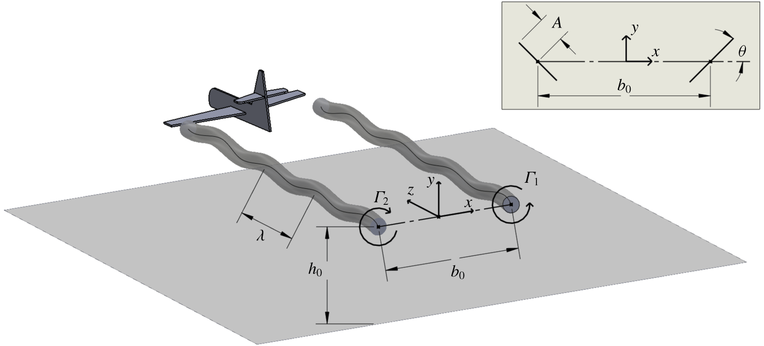
A schematic showing the key parameters governing the system and the coordinate system employed for the numerical study. The view in the  $x{-}y$ plane illustrates the planar projection of the vortex cores with both the amplitude and angle of the instability shown.

The structure of this article is as follows: first the problem definition and numerical approach are discussed in § 2; then the results from the direct numerical simulation concerning the evolution of the various modes of wall-bounded interaction follow in § 3; and the influence of the Reynolds number and the vortex core size is discussed in § 4. The article ends with conclusions in § 5.
2 Methodology
This section details the problems under investigation, defines the relevant parameters and discusses the computational method used to solve the governing equations.
2.1 Objective
This investigation considers the evolution of a pair of superimposed counter-rotating Lamb–Oseen-type vortices above a no-slip wall as shown in figure 1. The vortices are separated by an initial distance  $b_{0}$ and have characteristic core radius
 $a$. In two dimensions, the velocity fields of the vortices individually satisfy
 $$\begin{eqnarray}v_{\unicode[STIX]{x1D703}}(r)=\frac{\unicode[STIX]{x1D6E4}}{2\unicode[STIX]{x03C0}r}\left(1-\exp \left(-\frac{r^{2}}{a^{2}}\right)\right),\end{eqnarray}$$
where  $\unicode[STIX]{x1D6E4}$ is the circulation, and
 $r$ the radial distance from the vortex core. Note that the core radius
 $a$ is a function of time, and increases due to diffusion. In the case of an unbounded vortex, the evolution of the characteristic radius was shown by Batchelor (Reference Batchelor1967) to be
 $$\begin{eqnarray}a=\sqrt{a_{0}^{2}+4\unicode[STIX]{x1D708}t},\end{eqnarray}$$
where  $a_{0}$ is the initial characteristic radius and
 $\unicode[STIX]{x1D708}$ is the kinematic viscosity of the fluid. In the case of a vortex interacting with external vorticity, as is the case here where vorticity is generated on the no-slip wall, this equation provides an estimate to the evolution of the characteristic radius.
The parameters governing the evolution of an unbounded Lamb–Oseen vortex are hence the circulation  $\unicode[STIX]{x1D6E4}$ and the initial Reynolds number defined by the circulation through
 $Re=\unicode[STIX]{x1D6E4}_{0}/\unicode[STIX]{x1D708}$, where
 $\unicode[STIX]{x1D6E4}_{0}$ is the initial circulation. In the case of symmetric, parallel and unbounded counter-rotating vortices, both vortices translate under mutual induction in a straight line at constant speed
 $U=\unicode[STIX]{x1D6E4}/(2\unicode[STIX]{x03C0}b)$ normal to the plane on which the vortices lie. The time
 $t$ can thus be non-dimensionalised by the time taken for the vortex pair to descend a unit distance given the initial vortex spacing to define a non-dimensional time as
 $$\begin{eqnarray}\unicode[STIX]{x1D70F}=t\frac{\unicode[STIX]{x1D6E4}_{0}}{2\unicode[STIX]{x03C0}b_{0}^{2}}.\end{eqnarray}$$
It is important to note that the implicit length scale for the Reynolds number as defined in this article is based on the vortex spacing  $b$. This is consistent with the non-dimensionalisation of the time
 $\unicode[STIX]{x1D70F}$ and instability amplitude
 $A/b_{0}$ in the literature. If one is to consider the Reynolds number based on a natural velocity scale for a single vortex as
 $U_{a}=\unicode[STIX]{x1D6E4}_{0}/a_{0}$, one finds that the Reynolds number would be scaled by a factor of
 $a_{0}/b_{0}$ i.e.
 $Re_{a}=(a_{0}/b_{0})Re_{b}$. The experimental study of Asselin & Williamson (Reference Asselin and Williamson2017) quotes
 $Re_{a}$, but numerical studies typically assume
 $Re_{b}$. For consistency and simplicity, this article defines
 $Re=Re_{b}$, and
 $Re_{a}$ is used to distinguish the two scalings when discussing the experimental results.
This study seeks to provide further insight and analysis of the three modes of interaction identified in the experimental results of Asselin & Williamson (Reference Asselin and Williamson2017). As such, similar parameters were chosen, allowing both qualitative and quantitative comparisons to be drawn from the experimental results. It was found that the numerical results did not match the experimental results exactly for the parameters quoted in the experimental study. Upon further investigation, it was noted that the parameters were determined assuming reduced dependence of the measured azimuthal velocity about the centre point between vortices. A least squares fit to the data points suggested that the Reynolds number would be  $Re_{a}=732$ and
 $a_{0}/b_{0}=0.297$. However it is clear that the data near the centre point were ‘noisy’ and cannot be precisely modelled by the superposition of two Lamb–Oseen vortices. Furthermore, it is noted that the very small initial instability amplitude is subject to experimental error which is magnified over the exponential growth in the linear region. For this reason, a number of Reynolds number studies were necessary to investigate a parameter space for comparison to the experimental system (for details see § 4). A selection of Reynolds numbers and core sizes were hence considered, namely
 $Re=(1000,~1500,~2000,~2500)$ and
 $a_{0}/b_{0}=(0.4,~0.3,~0.23)$ to quantify variations in these parameters on the dynamics. The focus of this article is on
 $a_{0}/b_{0}=0.23$, which was chosen to be identical to the work of Leweke & Williamson (Reference Leweke and Williamson2011), and at
 $Re=2500$, recovers and explains the three modes of interaction identified by experiment.
A key governing parameter of the wall-bounded system was shown to be the amplitude of the long-wavelength perturbation to the initial vortex spacing  $A/b_{0}$. To capture the modes of the vortex pair–wall interaction, initial heights of
 $h_{0}/b_{0}=3.5,5.0,7.5$ and
 $10.0$ were examined, where
 $h_{0}$ is the initial distance of the vortex cores above the wall.
To study the instability of the vortex pair–wall interaction, an initial sinusoidal (displacement) perturbation is applied to the vortex cores at a  $\pm 45^{\circ }$ angle to the plane on which the vortices lie. After some experimentation, the initial amplitude of the instability for
 $Re=1000$ was set to
 $A_{0}/b_{0}=0.1$, for
 $Re=1500$ and for
 $Re=2000$ to
 $A_{0}/b_{0}=0.05$ and for
 $Re=2500$ to
 $A_{0}/b_{0}=0.01$, with an initial wavelength of
 $\unicode[STIX]{x1D706}=5.4$ in all cases. These parameters were determined a posteriori by ensuring that for a given initial height
 $h_{0}/b_{0}$, the amplitude of the perturbation
 $b_{0}$ above the wall matches the range observed in experimental visualisations. It is noted that the general evolution is not strongly dependent on the choice of initial amplitude
 $A_{0}/b_{0}$, but rather the amplitude of the instability upon strong wall interaction
 $A/b_{0}$. The evolution of the instability out of wall effect for small perturbations is approximated by linear theory (Widnall et al. Reference Widnall, Bliss and Zalay1971) and so long as the parameter
 $A/b_{0}$ is within the range for a given mode of vortex pair–wall interaction (see § 3), the initial amplitude does not hence significantly alter the dynamics. This is in accordance with the experimental results suggesting that
 $A/b_{0}$ is the primary governing parameter, and allows for comparisons to be drawn between the Reynolds numbers and core sizes despite the differences in the initial amplitude (see § 4).
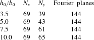
A schematic of the initial set-up with relevant parameters is shown in figure 1, and a table containing all of the relevant simulation controls is shown in table 1.
A summary of the major control parameters of the different cases studied. The primary study is the focus of the detailed discussion in § 3, and the additional studies are overviewed in § 4 to show that the results presented are not specific to a single choice of parameters. All of the studies are for  $\unicode[STIX]{x1D706}=5.4$.

2.2 Numerical formulation
The motion of an incompressible fluid is governed by the incompressible Navier–Stokes equations, which in non-dimensional form are expressed as
 $$\begin{eqnarray}\displaystyle & \displaystyle \unicode[STIX]{x1D735}\boldsymbol{\cdot }\boldsymbol{u}=0, & \displaystyle\end{eqnarray}$$
 $$\begin{eqnarray}\displaystyle & \displaystyle \frac{\unicode[STIX]{x2202}\boldsymbol{u}}{\unicode[STIX]{x2202}\unicode[STIX]{x1D70F}}=-\boldsymbol{u}\boldsymbol{\cdot }\unicode[STIX]{x1D735}\boldsymbol{u}-\unicode[STIX]{x1D735}p+\frac{2\unicode[STIX]{x03C0}}{Re}\unicode[STIX]{x1D6FB}^{2}\boldsymbol{u}, & \displaystyle\end{eqnarray}$$
where  $\boldsymbol{u}$ is the velocity scaled by
 $U_{0}=\unicode[STIX]{x1D6E4}_{0}/(2\unicode[STIX]{x03C0}b_{0})$,
 $\unicode[STIX]{x1D70F}$ is the time scaled by
 $2\unicode[STIX]{x03C0}b_{0}^{2}/\unicode[STIX]{x1D6E4}_{0}$ and
 $p$ is the kinematic pressure scaled by
 $U_{0}^{2}$. With the origin of a Cartesian coordinate system positioned at the midpoint of the two unperturbed vortex cores, the initial velocity field
 $\boldsymbol{u}_{0}$ is set to be the superposition of two perturbed Lamb–Oseen vortices with cores located at
 $\boldsymbol{R}_{p}=\pm b_{0}/2~\boldsymbol{e}_{x}+\unicode[STIX]{x1D71F}$, where
 $\boldsymbol{R}_{p}$ is the position vector of the vortex cores taken from the origin. The initial perturbation,
 $\unicode[STIX]{x1D71F}$, is set to be a sinusoidal wave with amplitude
 $A_{0}$ and wavelength
 $\unicode[STIX]{x1D706}$ such that
 $$\begin{eqnarray}\unicode[STIX]{x1D71F}=(A_{0}\cos \unicode[STIX]{x1D703})\sin \left(\frac{2\unicode[STIX]{x03C0}}{\unicode[STIX]{x1D706}}z\right)\boldsymbol{e}_{\mathit{x}}+(A_{0}\sin \unicode[STIX]{x1D703})\sin \left(\frac{2\unicode[STIX]{x03C0}}{\unicode[STIX]{x1D706}}z\right)\boldsymbol{e}_{y},\end{eqnarray}$$
where  $\unicode[STIX]{x1D703}$ is the angle to the plane of the pair. The long-wave instability was shown by Crow (Reference Crow1970) to occur at an angle of approximately
 $\unicode[STIX]{x1D703}=45^{\circ }$ to the plane of the pair, which is used to set up the initial three-dimensional velocity field.
The domain considered is a cuboid with boundaries located at  $-20b_{0}\leqslant x\leqslant 20b_{0}$,
 $-h_{0}\leqslant y\leqslant 16b_{0}$,
 $0\leqslant z\leqslant \unicode[STIX]{x1D706}$. The
 $x$ and upper
 $y$ domain bounds are set to be large enough such that the velocity remains close to that determined by the initial vortex dipole (extending the domain shows this to be the case). Axially periodic conditions for the velocity and pressure are applied at axial boundaries. A no-slip boundary condition is applied the wall and the velocities on top and lateral boundaries are prescribed by the initial velocity field of the vortex dipole.
Both the vorticity components and the  $Q$-criterion, where
 $Q$ is the second invariant of
 $\unicode[STIX]{x1D735}\boldsymbol{u}$, are used as aids to visualise the flow field and to identify vortex structures.
Vortex strength (or circulation),  $\unicode[STIX]{x1D6E4}$, is related to the vorticity by
 $\unicode[STIX]{x1D6E4}=\iint _{S}\unicode[STIX]{x1D714}\cdot \text{d}S$, with the integration taken over an area containing the vorticity
 $\unicode[STIX]{x1D714}$. This is quantitatively calculated in this study by integrating around contours at 1 % of the maximum vorticity on planes oriented normal to the axial direction.
The  $Q$-criterion requires a connected fluid region with a positive second invariant of
 $\unicode[STIX]{x1D735}\boldsymbol{u}$, such that
 $Q>0$ (Hunt, Wray & Moin Reference Hunt, Wray and Moin1988). This represents regions in the flow where rotation dominates strain. Visualisation of vortex structures with the flow are obtained by calculating the
 $Q$-field and plotting isosurfaces for
 $Q=0.001$. Minimum pressures within the
 $Q$-structures at the peak (
 $z=\unicode[STIX]{x1D706}/4$), trough (
 $z=3\unicode[STIX]{x1D706}/4$) and mid (
 $z=\unicode[STIX]{x1D706}/2$) planes are computed to study axial flow in the vortex pairs.
Vortex core locations are determined using the eigenmode based algorithm in Haimes (Reference Haimes2000). The issue with this approach is that the algorithm also locates patterns of strained flow, as in the boundary layer generated on the no-slip wall. The  $Q$-criterion is hence used to identify any spurious vortex cores.
The amplitude of the long-wavelength displacement type instability and the orientation of the plane on which it lies is found by planar projection of the vortex cores onto the  $z$ plane, and geometrically deducing the angle and amplitude. Note that the displacement of the vortex line is taken to be indicative of the amplitude of the instability, and not the exponential growth of the velocity perturbations.
2.3 Numerical method
A spectral-element method was employed to spatially discretise equations (2.4) and (2.5) in the cross-plane of the vortex pair. Lagrangian tensor-product polynomial basis functions are used within each element, using the fractional step approach discussed in Thompson et al. (Reference Thompson, Hourigan, Ryan and Sheard2006). The spatial polynomial interpolant functions, of which the polynomial degree order can be selected at run time to modify spatial resolution, are based on the quadrature points for Gauss–Legendre–Lobatto quadrature. The DNS technique further employs a Fourier expansion in the axial ( $z$) direction. Because the pressure and diffusion substeps are linear, the equation for each Fourier mode decouple, allowing these steps to proceed in parallel. The advection step uses an Adams–Bashforth approach in real space on a point by point basis. The three-dimensional variant and the method of parallelisation is described in more detail in Karniadakis & Triantafyllou (Reference Karniadakis and Triantafyllou1992).
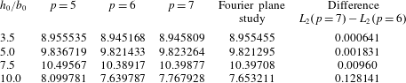
The number of macro-elements and Fourier planes used for the DNS study. This table does not include the internal spectral-element nodes, for which a convergence study (see table 3) is employed to ensure a grid independent solution.

High grid resolution was used for simulating the vortex pair–wall interaction. As indicated above, beyond the distribution of macro-elements within the domain (table 2), spatial resolution is further controlled through selection of the degree of the polynomial shape functions imposed on the macro-elements. For each grid investigated, the Lagrangian polynomial interpolant order was increased until convergence was achieved. The initial convergence criterion used was based on the  $L_{2}$ norm of the velocity field,
 $L_{2}=\int _{\unicode[STIX]{x1D6FA}}|\boldsymbol{u}|\,\text{d}\unicode[STIX]{x1D6FA}$ at
 $\unicode[STIX]{x1D70F}=20$, which was chosen as an appropriate scalar value that reflects the evolution of the system after the occurrence of wall interaction for all initial heights. The DNS predictions were considered effectively grid independent once the difference of the
 $L_{2}$ norm between successive grids fell to less than
 $2\,\%$.
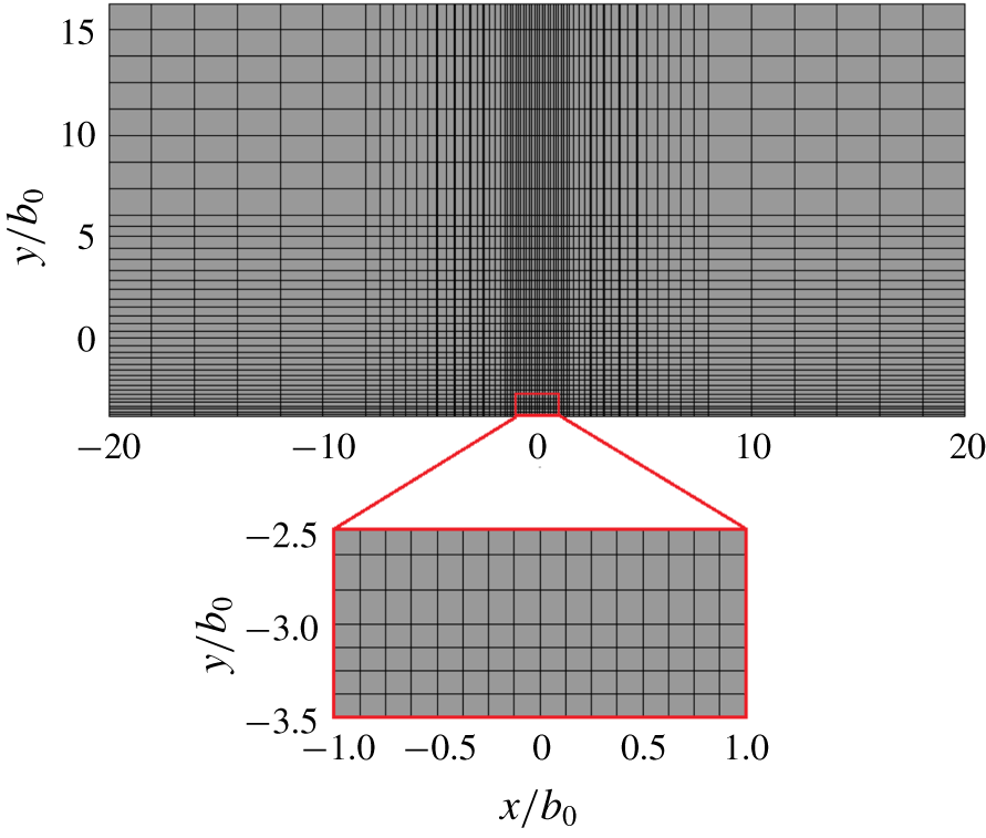
An example of the grid compression used for the DNS study for the case with  $h_{0}/b_{0}=3.5$. The grid is highly resolved in the region of vortex descent and near the no-slip wall. A close-up view of the compressed region is also illustrated. Only the macro-elements are shown with the DNS study employing 36 spectral nodes per macro-element.

Each grid tested was highly refined in the vicinity of the vortex pair for the entire integration time. Figure 2 shows a typical macro grid used for these studies, showing significant mesh compression in the region corresponding to vortex descent and near the ground plane.
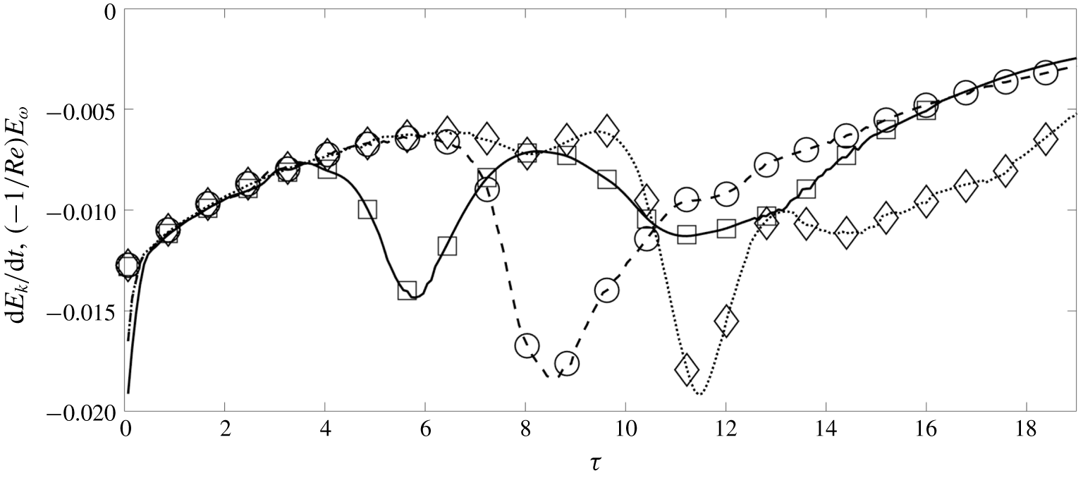
Validation study indicating that equation (2.7) is satisfied for all time steps of the solution for all three initial heights at  $Re=2500$. The lines (—), (- - -) and (
 $\cdots$) correspond to the decay of global kinetic energy and the symbols (
 $\Box$), (
 $\bigcirc$) and (
 $\diamondsuit$) correspond to the sign inverted global enstrophy scaled by the kinematic viscosity for
 $h_{0}/b_{0}=5,7.5$ and
 $10$ respectively. For visibility, the symbols are presented at intervals of
 $\unicode[STIX]{x1D6FF}\unicode[STIX]{x1D70F}=5/\unicode[STIX]{x03C0}$; however, the largest error is no larger than 2.0 % for all initial heights and
 $\unicode[STIX]{x1D70F}>0.4$, once the initial velocity field evolves to satisfy the governing equations.

In the spanwise direction, 144 Fourier modes were used to resolve the flow for all grids. This was decided on as the distance between spectral nodes in the region of mesh compression of the  $x$ and
 $y$ planes is approximately the same as the distance between Fourier planes in the
 $z$ direction. A convergence study at 192 Fourier planes for
 $p=6$ was considered, with the largest percentage error being
 ${\sim}0.18\,\%$ for
 $h_{0}/b_{0}=10.0$; 144 planes were hence considered sufficient for convergence and used for all studies.
A small time step of  $\unicode[STIX]{x1D6FF}\unicode[STIX]{x1D70F}=0.0025$ was used for all simulations, i.e. 400 time steps per convective time. As shown in table 3, the percentage difference in the
 $L_{2}$ norm at
 $\unicode[STIX]{x1D70F}=20$ for polynomial orders 6 and 7 is a maximum of
 $1.6\,\%$ for the largest initial height
 $h_{0}/b_{0}=10.0$. For all other heights, the percentage difference is of the order of
 $0.1\,\%$. With the numerical simulations revealing the production of intricate vortical structures of smaller and smaller scales with time (see § 3), a more physical a posteriori validation study was conducted to ensure a physical solution. In the case of no-slip walls, periodic boundary conditions, and lateral boundaries far from the vortices, as is the case here, it can be shown that the decay of the global kinetic energy in the numerical domain is proportional to the global enstrophy (Doering & Gibbon Reference Doering and Gibbon1995)
 $$\begin{eqnarray}\frac{\text{d}E_{k}}{\text{d}t}=-\frac{1}{Re}E_{\unicode[STIX]{x1D714}},\end{eqnarray}$$
where the global kinetic energy is given by  $E_{k}=\int _{\unicode[STIX]{x1D6FA}}\frac{1}{2}|\boldsymbol{u}|^{2}\,\text{d}\unicode[STIX]{x1D6FA}$ and the global enstrophy by
 $E_{\unicode[STIX]{x1D714}}=\int _{\unicode[STIX]{x1D6FA}}|\unicode[STIX]{x1D74E}|^{2}\,\text{d}\unicode[STIX]{x1D6FA}$. Figure 3 illustrates that equation (2.7) is satisfied for the various numerical simulations for
 $p=6$ and 144 Fourier planes to a maximum error of 2 % with the exception of small times where the initially imposed Lamb–Oseen velocity field rapidly changes to satisfy the governing equations. The results of the direct numerical simulations can hence be considered converged and are presented for a polynomial order of 6. As the largest Reynolds number of
 $Re=2500$ was employed for this resolution study, predictions for all lower Reynolds numbers are also considered converged for
 $p=6$.
Convergence study showing the  $L_{2}$ norm of velocity at
 $\unicode[STIX]{x1D70F}=20$ for various spectral polynomial orders
 $p$ for different initial heights. A polynomial order of
 $p=6$ is taken to be sufficiently converged for all studies. The Fourier plane convergence study is for 192 Fourier planes, with all other studies conducted with 144 Fourier planes.

3 Results
This section discusses the numerical solution to the vortex pair above a no-slip wall. Three modes of interaction were observed by experimental visualisations (Asselin & Williamson Reference Asselin and Williamson2017) depending on the initial height of the vortex pair above the wall. As will be shown, a defining insight of the numerical results is that the observation of Asselin & Williamson (Reference Asselin and Williamson2017) that vortex tongues reconnect to form vertical or horizontal rings is not supported by the DNS; here the modes are hence referred to as the ‘small-amplitude mode’, ‘large-amplitude mode’ and ‘large ring mode’, respectively.
This section is organised as follows: first, the evolution of the vortex strength (circulation) for the three modes is discussed, with the parallels and differences in the dynamics outlined. Second, a thorough discussion of the three modes follows, detailing the formation and evolution of secondary structures, the connection between the axial flow in the primary vortices to the dynamics and the long-term evolution of the flow to dissipation. Figures and supplementary movies (available at https://doi.org/10.1017/jfm.2019.816) illustrating the vortex structures are complemented by vorticity contours and streamlines at key cross-sections to better visualise the formation and trajectories of these structures. The small- and large-amplitude modes are compared to experimental visualisations of the vortex pair–wall interaction.
3.1 Vortex strength
The discussion concerning the strength of viscous vortex pairs in the wall effect is directly coupled to the dynamics and development of the long-wave instability. Despite the literature covering the development, growth and influence of the boundary layer vorticity in two dimensions, the axially perturbed vortex, as in the case of wing-tip vortices in ground effect, is not fully understood. This section seeks to relate the differences in a perturbed three-dimensional vortex to the existing literature, and to relate the dynamics of the vortex pair and the development of the instability to the evolution in the strength of the vortices.
An overview of the similarities in vortex strength evolution and physics between all modes of interaction is first discussed.
The size of individual vortices within counter-rotating vortex pairs increases as a function of time due to viscous diffusion. This results in increasing overlap between the vorticity distributions of the pair components, triggering cross-annihilation and a decrease in circulation of each vortex. The decrease in circulation progressively lowers the effective Reynolds number of the system, compounding the effect of viscosity on the evolution. As the vortex pair interacts with the wall, a boundary layer with opposite signed vorticity beneath each vortex further acts to strongly decrease the circulation through vorticity cross-diffusion, until the primary vortex ‘rebounds’. The formation of secondary vortices influences the circulation evolution through the action of vorticity annihilation between primary and secondary vortex structures, after which both the primary and secondary vortices diffuse through viscosity.
Moreover, the generation of secondary vorticity at the wall is a function of both the instantaneous distance of the primary vortex core above the wall  $h/b_{0}$, and the primary core radius
 $a$ when the vortex is in close proximity to the wall. As the Crow instability develops as an out-of-plane
 $(\unicode[STIX]{x1D703}\neq 0)$ sinusoidal wave in the axial direction, the distance of each vortex core to the wall is a function of the axial coordinate
 $z$. The respective decreases and increases in circulation of the primary and secondary vortices hence occur most strongly in the troughs of the Crow instability, and most weakly at the peaks.
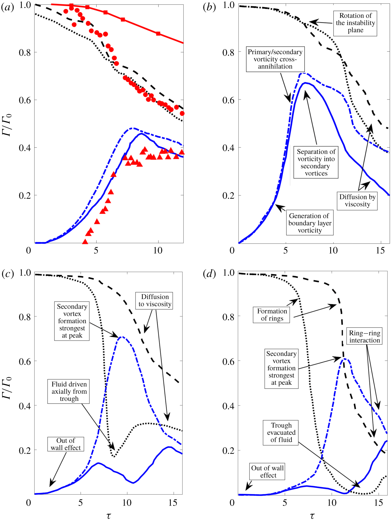
Naturally, the evolution in vortex circulation relates directly to the evolution of the vortex structures observed in the DNS. The variation in the evolution between different initial heights gives credence to the three modes of interaction identified by experiment. A key similarity between all modes of interaction is the evolution up to and including the initial primary vortex–wall interaction. This phase consists primarily of an out-of-wall effect, where the Crow instability develops at an angle of approximately  $\unicode[STIX]{x1D703}=48^{\circ }$, and viscous diffusion and primary vortex interaction dominates circulation loss in the primary vortex pair, consistent with studies on unbounded vortex pairs (Buntine & Pullin Reference Buntine and Pullin1989). Upon subsequent wall interaction, vorticity at the lower boundary gives rise to a boundary layer, where the circulation of the secondary vorticity begins to grow. The shear layer is initially localised to regions on the wall directly beneath the vortex cores, but then spreads outwards to enforce the no-slip boundary condition as the vortices descend further.
Once the adverse pressure gradient in the boundary layer is strong enough, roll up of the secondary vorticity into discrete vortex structures occurs, as discussed by Harvey & Perry (Reference Harvey and Perry1971). The subsequent development of the secondary vortex causes the primary vortices to rise and the secondary vortex begins to spiral around the primary vortex due to its lower circulation. The increase in wall-bounded vorticity is arrested by the formation of a discrete vortex, and viscous diffusion between vortex structures once again dominates the decrease in primary vortex strength.
Circulation of the primary and secondary vortices as a function of time taken by integrating around contours at 1 % of the maximum vorticity on planes oriented normal to the axial direction. The circulations at the initial troughs and peaks are shown for various initial starting heights and Reynolds numbers of the vortices, namely: (a)  $h_{0}/b_{0}=5.0$,
 $Re=1000$; (b)
 $h_{0}/b_{0}=5$,
 $Re=2500$; (c)
 $h_{0}/b_{0}=7.5$,
 $Re=2500$; and (d)
 $h_{0}/b_{0}=10$,
 $Re=2500$. The black dashed line (– – –) represents the peak circulation of the primary vortex, the black dotted line (
 $\cdots \cdots$) the trough circulation of the primary vortex, the blue dash-dot line (
 $-\cdot -\cdot -\cdot$) the peak circulation of the secondary vorticity and the blue solid line (——) the trough circulation of the secondary vorticity. The red markers are taken from Asselin & Williamson (Reference Asselin and Williamson2017); red squares for the unbounded instability, the red circle for the primary vortex circulation and the red triangles the secondary vorticity circulation. The sign of the secondary vorticity circulation is reversed.

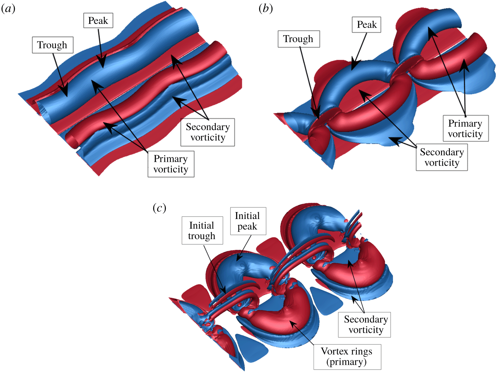
Vorticity at the level of  $0.01|\unicode[STIX]{x1D714}_{z_{max}}|$, illustrating the onset of the wall interaction in the three-dimensional Crow instability for the initial heights and corresponding times of (a) the small-amplitude mode,
 $h_{0}/b_{0}=5.0$,
 $\unicode[STIX]{x1D70F}=6.37$, (b) the large amplitude mode,
 $h_{0}/b_{0}=7/5$,
 $\unicode[STIX]{x1D70F}=7.16$ and (c) the large ring mode,
 $h_{0}/b_{0}=10.0$,
 $\unicode[STIX]{x1D70F}=11.14$ at
 $Re=2500$. The trough and peak regions of the modes and primary/secondary vorticity are annotated. Note the significant variation in vorticity annihilation at the troughs of the instabilities. Two wavelengths are shown for clarity. Positive vorticity is shown in red, negative in blue.

This discussion continues with the key differences in vortex strength between initial starting heights corresponding to the different modes of interaction.
At low Reynolds numbers, where the amplitude of the instability does not grow enough for there to be significant three-dimensional effects, the numerical results can be directly compared to the experimental quasi-two-dimensional results of the wall-bounded instability (Asselin & Williamson Reference Asselin and Williamson2017) (see figure 4a). At larger Reynolds numbers and initial heights of  $h_{0}/b_{0}=5.0$ above the wall (see figure 4b), the difference in circulation between peak and trough cross-sections is small relative to the other modes of interaction. An interesting observable phenomenon is the ‘crossing over’ of the peak and trough circulations of the primary vortex pair in figure 4(b). The initial ‘cross-over’ is due to the rotation of the instability plane, as shown with DNS in § 3.2. The second ‘cross-over’ is related to the viscous annihilation between the primary vortex and the formation of secondary vortex ‘tongues’, which remain closer to the primary vortex pair at the initial peak. In the low Reynolds number study (figure 4a), the onset of three-dimensional effects are noticeable but significantly less pronounced; the rotation of the instability plane results in the peak and trough circulation almost meeting and vortex tongues do not form (see § 4).
As the amplitude of the Crow instability grows, the relative changes in distance between the troughs and peaks of both primary vortices and the wall result in significantly stronger vorticity annihilation at the trough.
Illustrated in figure 5 are the differences between the initial heights upon wall interaction; note the significant variation in vortex interaction at the trough between the three modes. At initial heights of  $h_{0}/b_{0}=7.5$ above the wall (see figure 4c), the circulation at the trough of the primary vortex is observed to fall rapidly relative to the peak, and the secondary vortex does not fully form at the trough before rotating inwards towards the peak (see § 3.3 for more details). The primary circulation at the trough, however, recovers slightly during the rebound as the primary vortices are driven away.
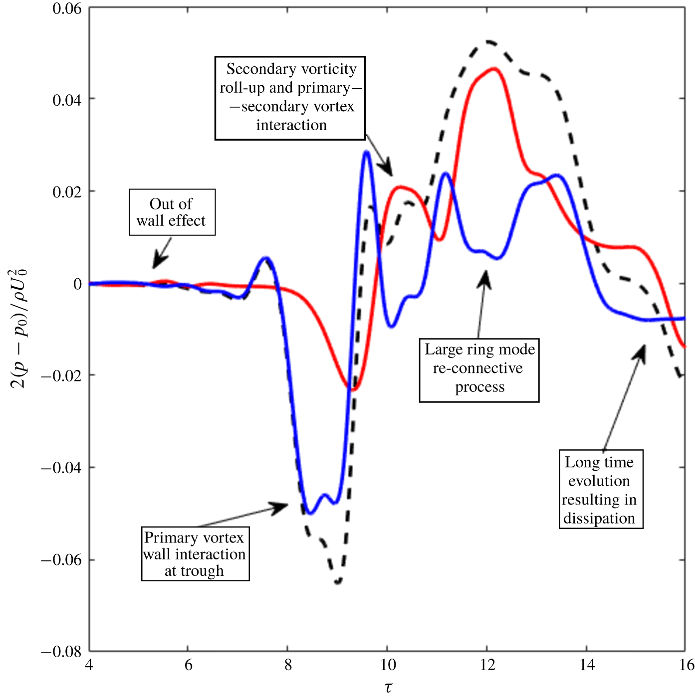
The evolution in circulation is similar at large initial heights where the Crow instability forms rings as shown in figure 4(d) for  $h_{0}/b_{0}=10.0$. In this case, however, the circulation at the trough of the primary vortex instability falls to near zero, with a vortex ‘bridge’ (for more details see § 3.4) containing the entirety of the remaining circulation. The circulation at the peak also falls well below that of the
 $h_{0}/b_{0}=7.5$ case, with the secondary circulation at the peak growing to be stronger than that of the primary pair. A slight recovery in the circulation of the primary pair at the trough is observed at large times due to ring–ring interaction at the trough.
It is clear from figures 4 and 5 that three-dimensionality clearly plays a key role in the influence of a wall on the vorticity cancellation of the strained vortices, which can be directly related to the evolution of the vortex pair. The current body of literature has not considered the influence of three-dimensionality and although the results presented in this paper give an indication to its importance, a detailed study would give more insight into wall-bounded vortex flows.
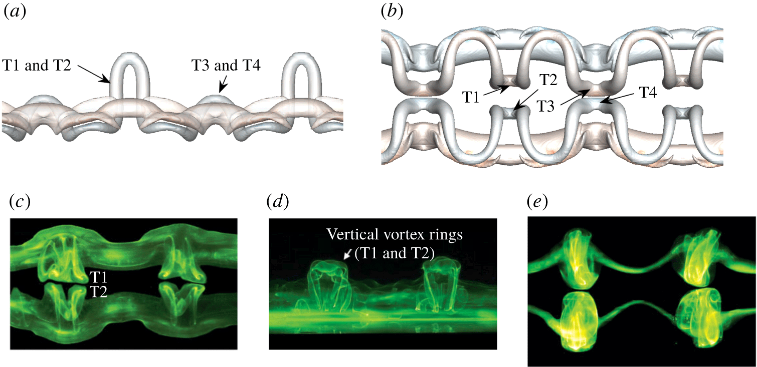
A comparison between experimental and numerical results for the small-amplitude mode. Panels (a,b) show the  $x{-}z$ and
 $y{-}z$ views of isosurfaces of vorticity magnitude
 $|\unicode[STIX]{x1D6FA}|=0.005$ for
 $Re=2500$,
 $a_{0}/b_{0}=0.23$ and at
 $\unicode[STIX]{x1D70F}=10.35$. Two wavelengths of
 $\unicode[STIX]{x1D706}=5.4$ are shown. Panels (c,d) show the laser illuminated dye of the secondary vorticity in the same views at
 $\unicode[STIX]{x1D70F}=12.0$, and (e) shows the laser illuminated dye of the primary vorticity in the
 $x{-}z$ plane at
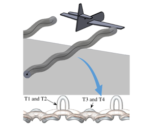
 $\unicode[STIX]{x1D70F}=12.0$. Panels (c,d) are reproduced with permission of Asselin & Williamson (Reference Asselin and Williamson2017). Vortex ‘tongues’ are labelled T1–T4.

3.2 Small-amplitude mode
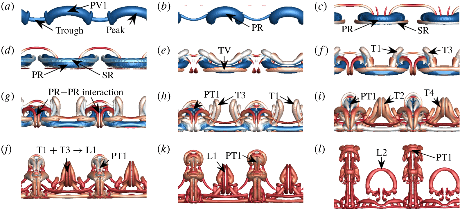
Depending on the extent of the instability, three modes of interaction between a descending counter-rotating vortex pair interacting with a wall were identified. Experimental visualisations of the perturbed vortex pair system interacting with a wall at small perturbation amplitudes identified the formation of two vertically oriented vortex tongues (T1 and T2 in figure 6c), which were conjectured to form vertically oriented vortex rings (figure 6d). These structures were observed to interact at the symmetry plane and form secondary vertical loops.
A discussion of the results identified by experiments that result in these vertical rings is first provided. Physical arguments together with support of the DNS results suggest that vertical rings do not form as reconnection does not occur near the ground plane. Furthermore, more sets of tongue-like structures not observed by experiment are captured by DNS for smaller core sizes upon three-dimensional rebound of the vortex pair (T3 and T4 in figure 6a,b). The study discussed here is at  $Re=2500$,
 $a_{0}/b_{0}=0.23$,
 $h_{0}/b_{0}=5$ and
 $A_{0}/b_{0}=0.01$ resulting in an amplitude one vortex spacing above the ground plane of
 $A/b_{0}=0.1371$. This is consistent with the vertical rings mode predicted experimentally to occur between
 $0.1\leqslant A/b_{0}\leqslant 0.3$ (Asselin & Williamson Reference Asselin and Williamson2017). A comparison between the experimental results and the current study is presented in figure 6.
This section is organised as follows: initially, a discussion of the orientation of the instability is presented, and the evolution of the small-amplitude mode made explicit; then, the growth and inhibition of the wall-bounded three-dimensional Crow instability is discussed; finally the pressure distribution resulting in axial flow in the primary vortex is examined, and related to the evolution of the vortical structures.
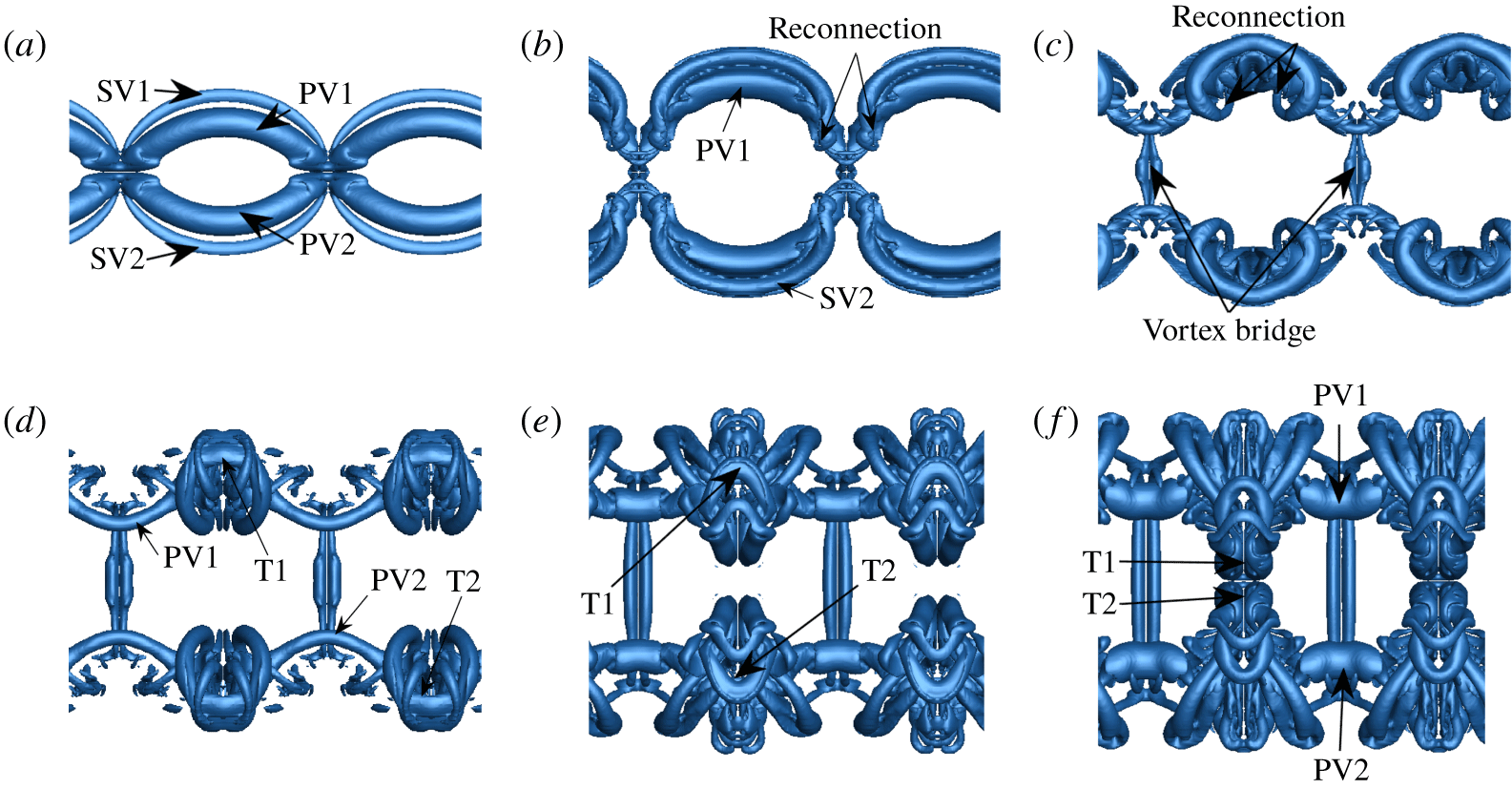
The evolution of the small-amplitude mode projected onto the  $x{-}z$ plane, here pictured for
 $Re=2500$,
 $a_{0}/b_{0}=0.23$ and
 $h_{0}/b_{0}=5.0$. The times for the snapshots are as follows: (a)
 $\unicode[STIX]{x1D70F}=5.25$; (b)
 $\unicode[STIX]{x1D70F}=7.64$; (c)
 $\unicode[STIX]{x1D70F}=8.75$; (d)
 $\unicode[STIX]{x1D70F}=10.42$; (e)
 $\unicode[STIX]{x1D70F}=11.54$; (f)
 $\unicode[STIX]{x1D70F}=14.16$; (g)
 $\unicode[STIX]{x1D70F}=17.03$; (h)
 $\unicode[STIX]{x1D70F}=21.09$; (i)
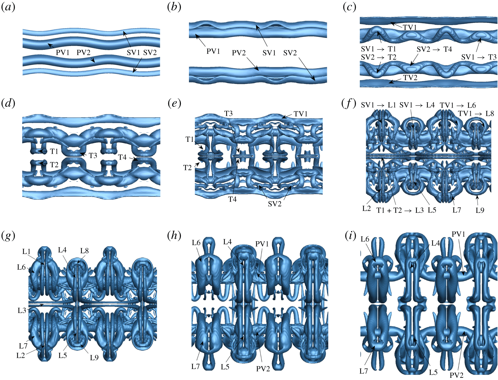
 $\unicode[STIX]{x1D70F}=27.05$. The labels PV, SV and TV refer to primary, secondary and tertiary vortices respectively; the labels T1–T4 refer to the vortex tongues and the labels L1–L9 refer to the ‘loop-like’ structures identified and discussed in the text. The supplementary movie (movie 1) animates the evolution and is extremely helpful for visualisation.

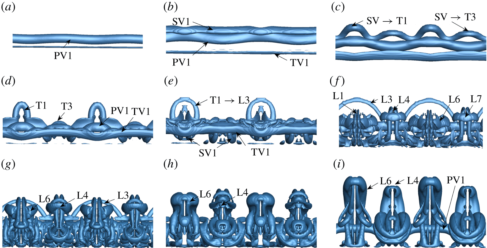
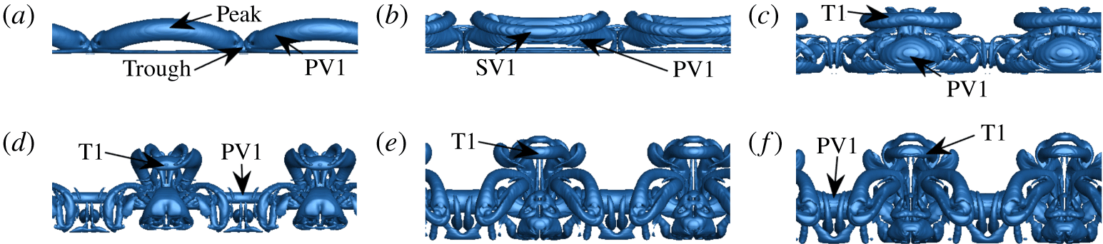
As the primary vortex pair approaches the wall (PV1 and PV2 in figures 7a and 8a), the vortices entrain the surrounding fluid and generate a thin boundary layer at the wall. Upon approach, the orientation of the instability plane begins to rotate; this is critically important as it dictates the dynamics underlying the formation of the vortex tongues. The vortex pair continues to move closer to the wall, the vortices begin to separate, and the boundary layers undergo rapid separation and growth (see figures 7b and 8b). The adverse pressure gradient generated at the wall by the primary vortices acting on the region of local vorticity concentration within the boundary layer results in the formation and separation of secondary vortices (SV1 and SV2) from the ground plane. The secondary vortices induce an upwards velocity on the primary vortices, resulting in the well-researched ‘rebound’, seen clearly between figures 8(a) and 8(b). Upon ‘rebound’ of the primary vortex following the roll-up of the secondary vorticity, the arresting vortex detaches from the wall and is advected around the primary vortex by induction caused by unequal strength vortex interaction. Unlike the two-dimensional wall-bounded Crow instability, however, regions of the primary vortices, being situated closer to the wall, result in the initial localised formation of these secondary vortices. This gives rise to the characteristic vortex tongues pictured in figures 6 to 8, labelled T1 through T4. Two primary vortex tongues (T1 and T2) are formed per wavelength at the initial trough of the instability and grow at significantly faster rates when compared to the cooperative (Crow) instability (see figure 8d). A pair of secondary tongues (T3 and T4) form in the vicinity of the initial peak of the primary vortex instability (figure 7d), resulting in four tongues per instability wavelength. The isolated vortex tongue development is presented in figure 9. The vortical structures formed resemble hairpin vortices and are remarkably similar to the structures observed by Cheng et al. (Reference Cheng, Lou and Luo2010) under oblique ring–wall impingement.
The evolution of the small-amplitude mode projected onto the  $x{-}y$ plane, here pictured for
 $Re=2500$,
 $a_{0}/b_{0}=0.23$ and
 $h_{0}/b_{0}=5$. The times for the snapshots are as follows: (a)
 $\unicode[STIX]{x1D70F}=5.25$; (b)
 $\unicode[STIX]{x1D70F}=7.64$; (c)
 $\unicode[STIX]{x1D70F}=8.75$; (d)
 $\unicode[STIX]{x1D70F}=10.42$; (e)
 $\unicode[STIX]{x1D70F}=11.54$; (f)
 $\unicode[STIX]{x1D70F}=14.16$; (g)
 $\unicode[STIX]{x1D70F}=17.03$; (h)
 $\unicode[STIX]{x1D70F}=21.09$; (i)
 $\unicode[STIX]{x1D70F}=27.05$. See figure 7 for further information.

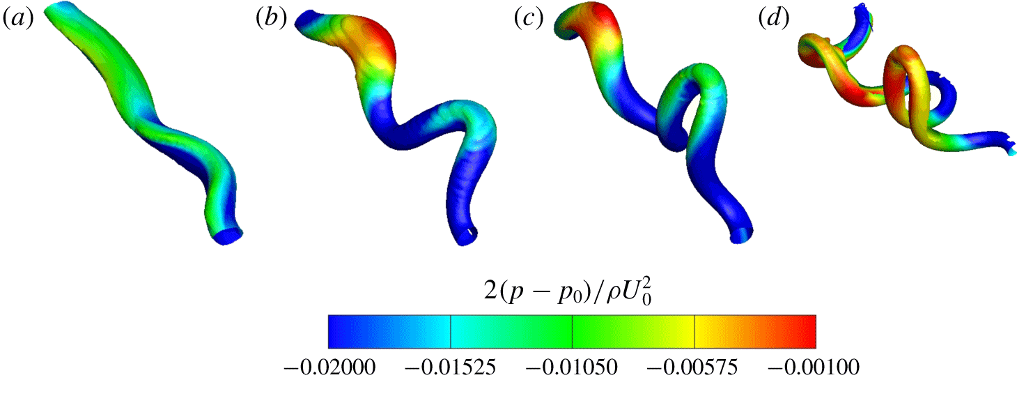
Contours of pressure on  $Q$-criterion isosurfaces of the secondary vortex for the small-amplitude mode at
 $Re=2500$,
 $h/b_{0}=5.0$ and
 $a_{0}/b_{0}=0.23$, shown here for one wavelength. Local pressure variations give an indication to the axial flow development in the secondary vortices. The colours correspond to increasing pressure in the following order: blue, green, yellow, red. The times for the snapshots are as follows: (a)
 $\unicode[STIX]{x1D70F}=7.96$; (b)
 $\unicode[STIX]{x1D70F}=8.36$; (c)
 $\unicode[STIX]{x1D70F}=9.15$; (d)
 $\unicode[STIX]{x1D70F}=10.35$.

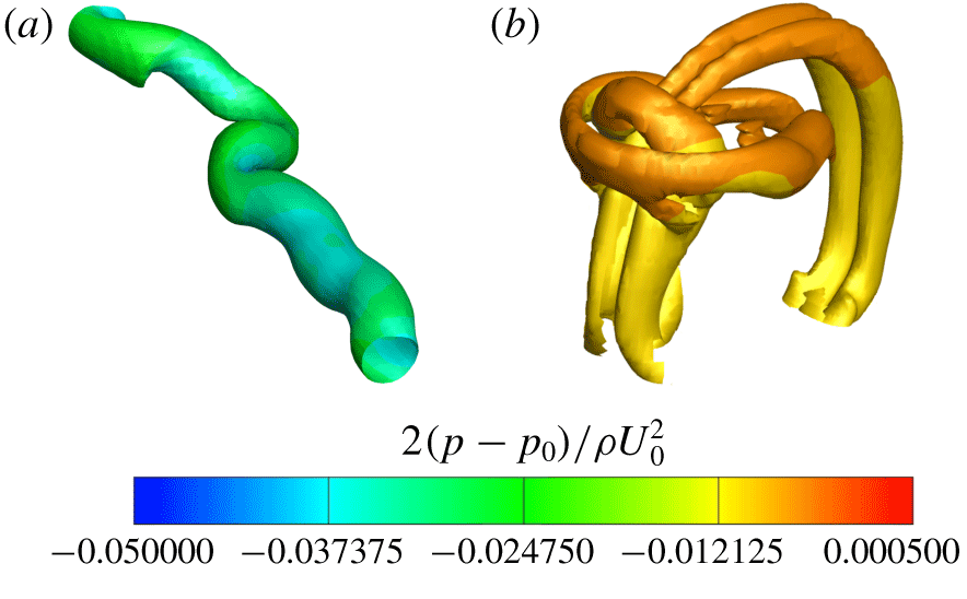
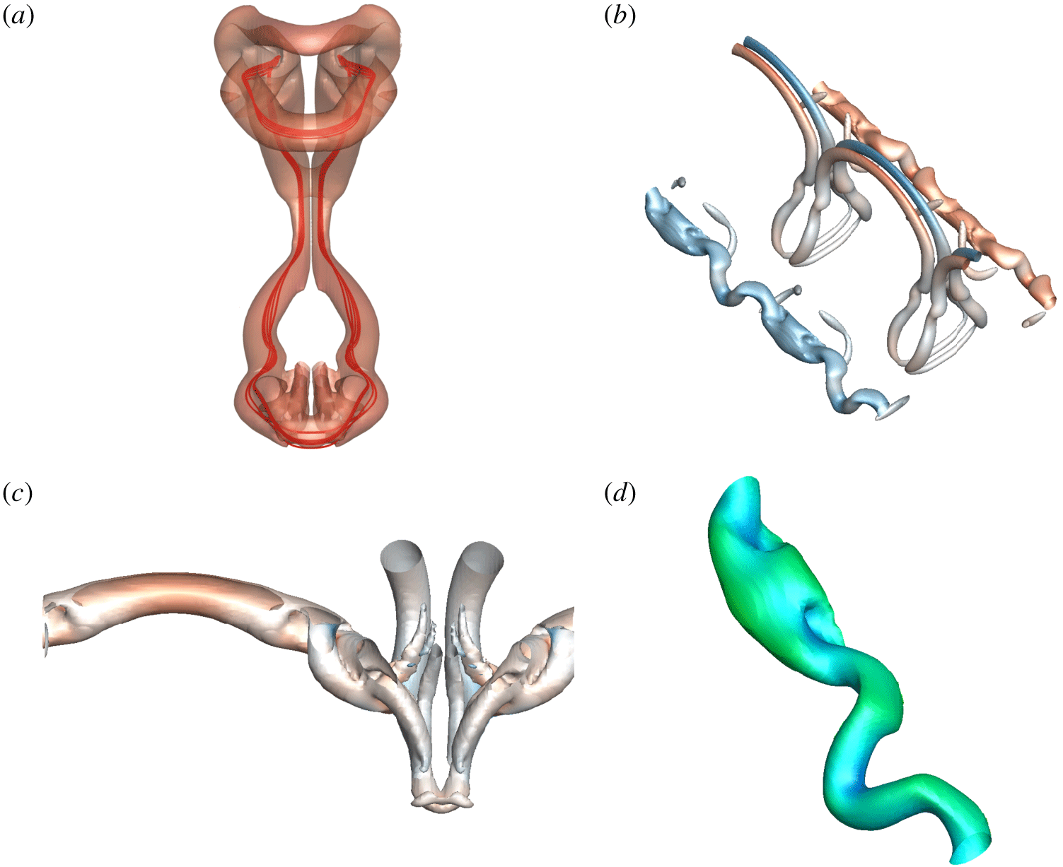
Contours of pressure on  $Q$-criterion isosurfaces illustrating (a) the long-term evolution of the primary vortex at
 $\unicode[STIX]{x1D70F}=27.85$ and (b) the secondary/tertiary dual-loop structures at
 $\unicode[STIX]{x1D70F}=15.92$ of the small amplitude mode. The pressure contour colours range from blue to green to red relative to the minimum and maximum pressures of the solution at the given times.

The differences in topology between the tongue pairs is directly influenced by the physics underlying their formation. The formation of the vortex tongues from the secondary vortex is shown in figure 9, with the pressure contours illustrating the strong axial flows away from the tongue tips further driving the rise of tongues. The formation of the large tongues (T1 and T2) occur at the initial troughs of the instability, whereby the large vorticity gradients cause locally higher pressure and drive axial flow away from the tip of the tongue (figure 9a). The smaller tongues (T3 and T4) form during the ‘rebound’ due to the rotation of the instability plane at the initial peak of the Crow instability. After the rebound, increased local vorticity annihilation between the primary and secondary vortex pair due to their relative proximity results in a ‘flattened’ vortex tongue profile (figure 9b). Both loops vertically orient prior to moving towards the plane of symmetry as in figure 9(c). Upon separation of the secondary vortex from the ground plane, tertiary vortical structures are generated, as observed in two-dimensional studies (cf. Kramer et al. Reference Kramer, Clercx and van Heijst2007). The bottom of the loops continue to advect about the primary vortex, and are stretched to the point of weak interaction with tertiary vortices (TV1 and TV2 in figure 7e). The secondary vortex remains connected as it is stretched around the primary vortex, and begins to form sets of loop-like structures (L1, L2, L4 and L5) around the primary vortex pair (figures 7f and 8f).
Thereafter, the two pairs of vortex tongues (T1–T2 and T3–T4) interact at the symmetry plane also forming loop-like structures (L3 in figures 7f and 8f). The secondary vortex loops both experience higher local viscous diffusion at the symmetry plane due to their interaction, and the vortices stretch radially outwards, ultimately resulting in a topologically complex flow. The complex dynamics that follows is an integral sum of influence by the relative orientation, distance and circulation of a given segment of a vortex relative to all other segments. For instance, sections of the secondary vortex core parallel to the primary vortex (oriented in the spanwise direction) are stretched further around the primary vortex core than non-parallel sections; this results in further amplification of the ‘tongue-like’ topology (figures 7f–h and 8f–h). Under these interactions, the secondary vortex wraps entirely about the primary vortex, and the tongues interact with one another to form ‘loop-like’ structures consisting of two counter-rotating vortex structures (L1, L2, L4 and L5 illustrated in figure 10b). In turn, the tertiary vortices (TV1 and TV2) wrap about these secondary vortex loops to form horizontally oriented loop-like structures (L6, L7, L8, L9 in figures 7g and 8g).
Ultimately, the secondary vortex loops at the symmetry plane dissipate under vorticity annihilation and viscous diffusion (figures 7h and 8h). The large-time evolution of the wall generated flow primarily consists of both secondary (L4 and L5) and tertiary (L6 and L7) ‘loop-like’ structures alongside the pair of primary vortices (PV1 and PV2), shown in figures 7(i) and 8(i). These structures ultimately interact with the symmetry plane and diffuse by viscosity, with the long-term evolution resulting in the two primary vortices (PV1 and PV2) primarily bent and twisted at the location corresponding to the initial peak of the Crow instability, illustrated in figure 10(a).
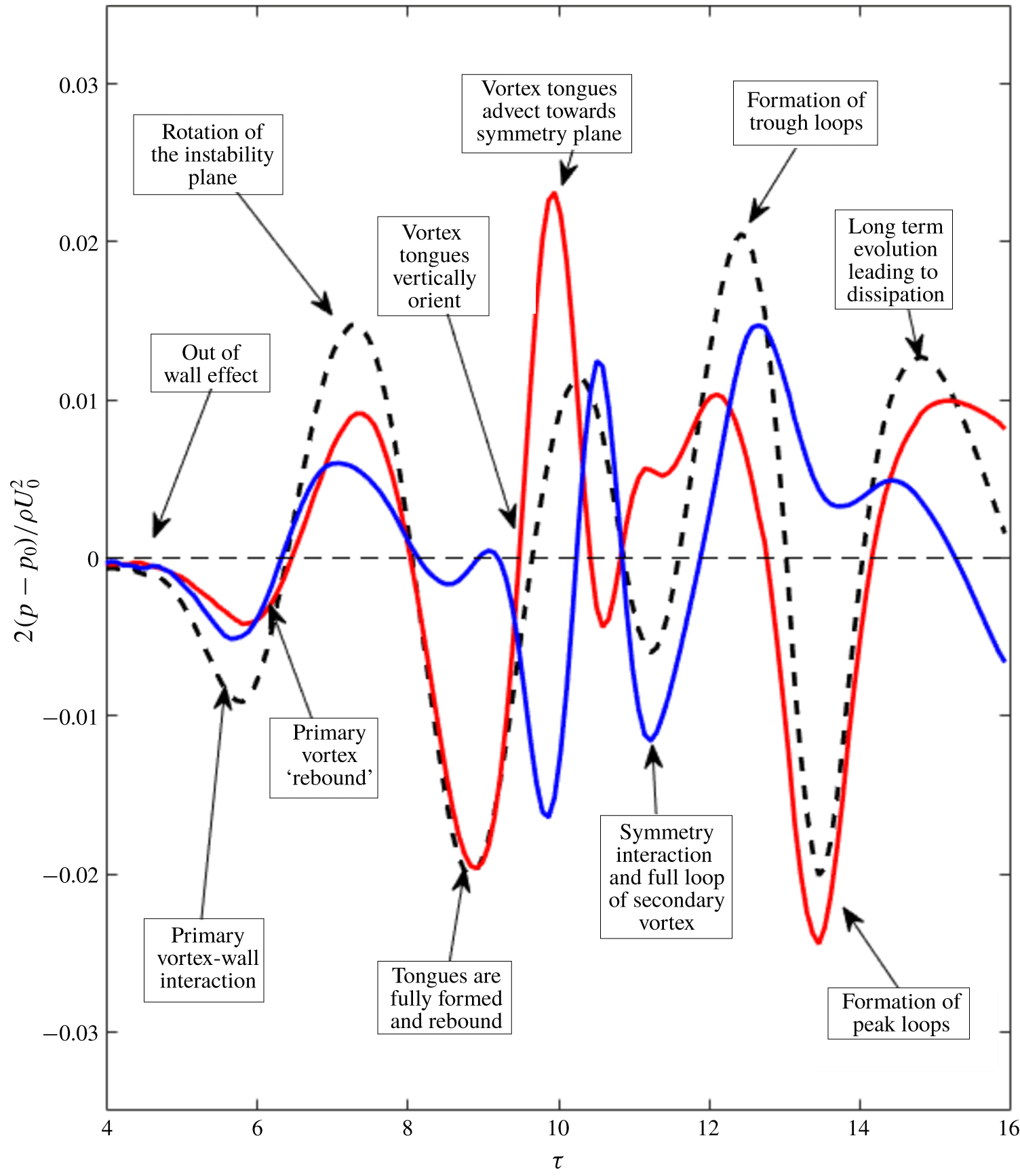
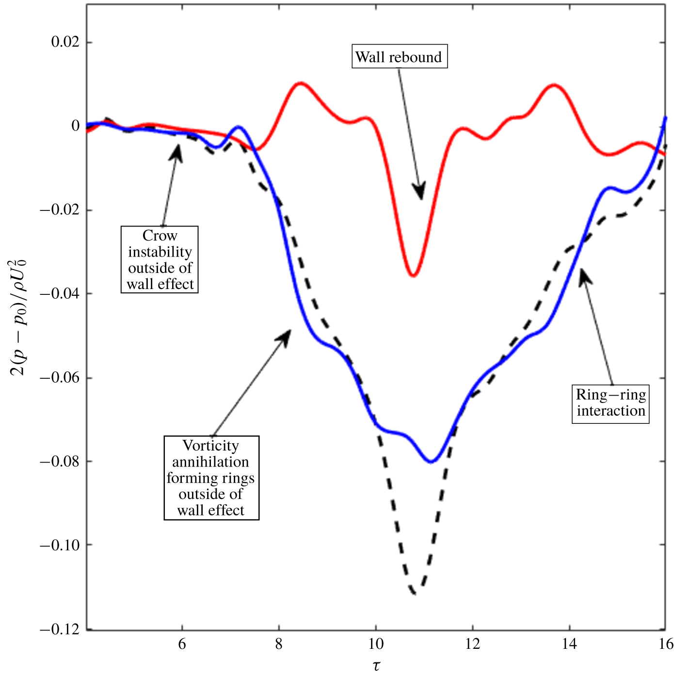
The dynamics of the vortex system can be further understood through the lens of the pressure distribution in the primary pair, which gives an indication of the axial flow in the vortices and its connection to the dynamics of the instability in wall effect. As regions of the vortex core closest to the wall experience larger viscous annihilation, this locally raises the pressure of the fluid, driving fluid away axially within the vortices. The evolution in pressure differential between the peak, mid-plane and trough of the instability, and the connection to the evolution discussed is illustrated in figure 11.
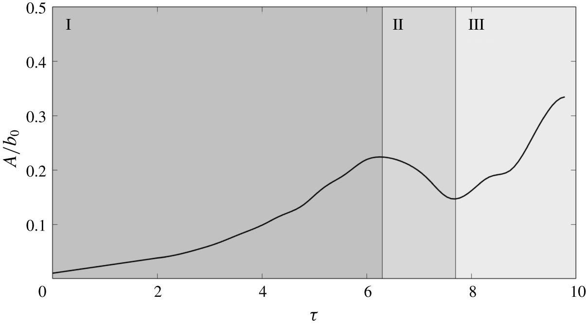
An additional interesting feature of the small-amplitude mode is the inhibition in the growth of the Crow instability observed by experiment (Asselin & Williamson Reference Asselin and Williamson2017). The numerical prediction of the evolution in the amplitude of the instability in the primary vortex pair illustrates both the inhibition of the ring development and the vortex ‘collapse’ visualised by Asselin & Williamson (Reference Asselin and Williamson2017).
The characteristic growth curve of the small-amplitude mode is shown in figure 12. The amplitude of the Crow instability  $A/b_{0}$ grows in accordance with linear theory until inhibited by the nonlinear ground effect near
 $\unicode[STIX]{x1D70F}\approx 5.5$. As the secondary vorticity separates from the ground plane and forms a discrete vortex, the formation of rings is further inhibited by the induced velocity of the secondary vortices on the primary pair, and grows to ultimately result in the radial arrest
 $(\unicode[STIX]{x1D70F}\approx 5.91)$ and decrease in the amplitude of the instability until
 $\unicode[STIX]{x1D70F}\approx 8.75$.
The onset of both nonlinear inhibition (II) and vortex ‘collapse’ (III) is now explained. The trough of the Crow instability interacts with the ground plane first, resulting in the localised generation of secondary vorticity. The resultant secondary vortex induces a locally restoring velocity on the primary pair; the instability is hence inhibited, and the amplitude of the distance between peak and trough is driven downwards. Strong axial flow due to pressure gradients (see figure 11) arising from the relative distance from the primary vortex pair to the ground plane, alongside the formation of the vortex tongues, results in the eventual loss of spanwise uniformity, visualised by experiment as vortex ‘collapse’ (see figure 6 for experimental visualisation of the ‘collapsed’ vortex). The instability during the collapse of the primary vortex is non-planar, and the amplitude is taken by projection onto the  $x{-}y$ plane. The local spanwise deformation of the vortex tube hence coincides with an increase in the plane-projected amplitude of the Crow mode. Unlike the unbounded Crow instability, which forms rings, this region is hence associated with an indication of vortex ‘collapse’ rather than an acceleration of the Crow instability. The evolution in the amplitude of the instability; illustrating both the non-planarity and the loss of spanwise uniformity of the third region, is further visualised in figure 13.
Pressure differential of the vortex pair for the small amplitude mode at  $Re=2500$ and
 $a_{0}/b_{0}=0.23$ illustrating the axial flow evolution in the primary vortices. The lines represent pressure differentials between the following cross-sections: the dashed line (- -) between the peak and trough; the red line (——) between the peak and mid-plane and the blue line (——) between the mid-plane and trough. The supplementary movie (movie 1 at https://doi.org/10.1017/jfm.2019.816) animates the evolution and is extremely helpful for comparison with this figure.

The Crow instability in ground effect for the small amplitude mode, here plotted for  $Re=2500$ and
 $h_{0}/b_{0}=5.0$. The amplitude of the displacement type instability is shown as a function of time, and three regions are identified, namely (I) linear growth, (II) nonlinear inhibition due to secondary vortex formation leading to radial arrest and (III) vortex breakdown due to strong axial flows. The amplitude is geometrically determined through planar projection of the vortex core line onto the axial plane.

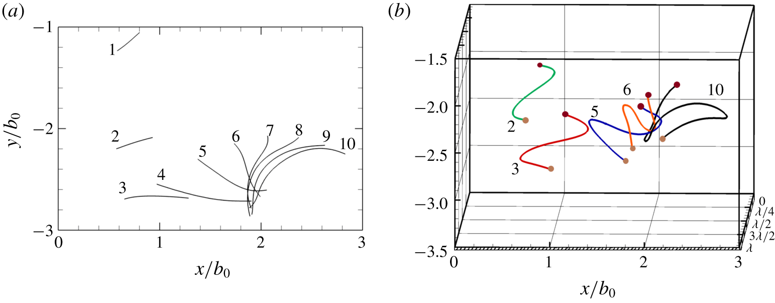
Visualisation of the evolution of the instability in time, here plotted for  $h_{0}/b_{0}=3.5$,
 $Re=1000$,
 $a_{0}/b_{0}=0.4$. (a) The projection of the instability cores onto the
 $x{-}y$ plane, with curvature indicating an out of plane instability. (b) Three-dimensional view of the development of the orientation of the instability with time. The maroon circles are at
 $z=0$ and the brown circles at
 $z=\unicode[STIX]{x1D706}$ to indicate depth. The numerals correspond to the non-dimensionalised time steps as follows: 1,
 $\unicode[STIX]{x1D70F}=1.59$; 2,
 $\unicode[STIX]{x1D70F}=3.18$; 3,
 $\unicode[STIX]{x1D70F}=4.77$; 4,
 $\unicode[STIX]{x1D70F}=6.37$; 5,
 $\unicode[STIX]{x1D70F}=7.96$; 6,
 $\unicode[STIX]{x1D70F}=9.55$; 7,
 $\unicode[STIX]{x1D70F}=11.14$; 8,
 $\unicode[STIX]{x1D70F}=12.73$; 9,
 $\unicode[STIX]{x1D70F}=14.32$; 10,
 $\unicode[STIX]{x1D70F}=15.92$.

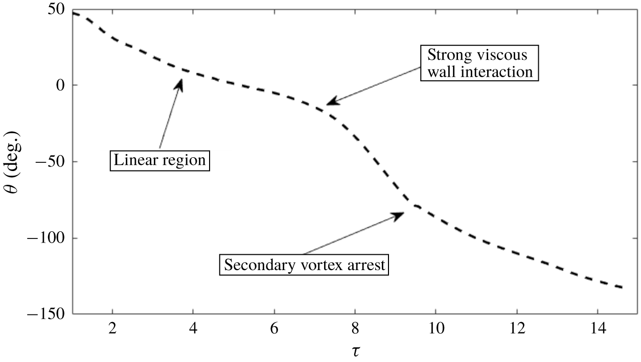
The orientation of the instability for the small amplitude mode, here illustrated for  $h_{0}/b_{0}=3.5$,
 $Re=1000$ and
 $a_{0}/b_{0}=0.4$. The instability plane rotates until viscous effects result in a non-planar instability.

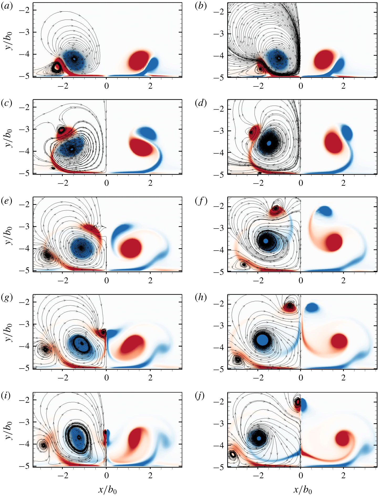
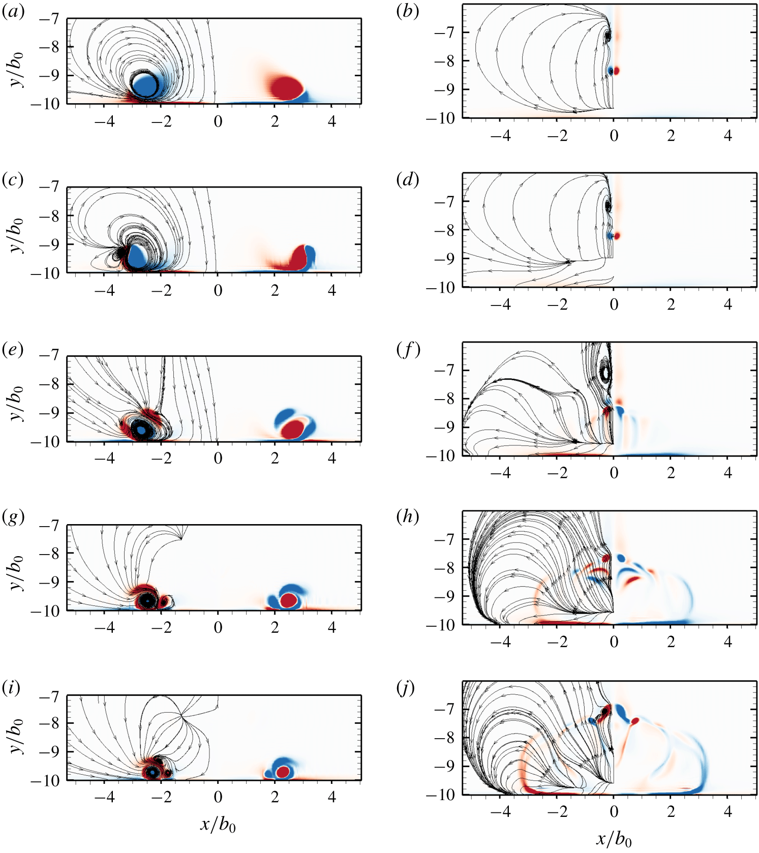
The  $z$ component of vorticity contours at cross-sections of the initial peak of the instability,
 $z=\unicode[STIX]{x1D706}/4$ (pictured in the left column) and the initial trough of the instability,
 $z=3\unicode[STIX]{x1D706}/4$ (pictured in the right column) for the small-amplitude mode at different times, here pictured for
 $Re=2500$,
 $h_{0}/b_{0}=5.0$ and
 $a_{0}/b_{0}=0.23$. Instantaneous streamlines are shown for half the domain and are symmetric about
 $x/b_{0}=0$. Red indicates positive vorticity, blue indicates negative vorticity. The times for the snapshots are as follows: (a,b)
 $\unicode[STIX]{x1D70F}=3.18$; (c,d)
 $\unicode[STIX]{x1D70F}=3.98$; (e,f)
 $\unicode[STIX]{x1D70F}=4.77$; (g,h)
 $\unicode[STIX]{x1D70F}=5.17$; (i,j)
 $\unicode[STIX]{x1D70F}=5.57$.

The plane on which the instability grows plays a critical role in the evolution of the small-amplitude mode and is now discussed.
The instability remains almost entirely planar until the ‘rebound’ of the primary vortex occurs, and the vortex cores begin to separate and bend. This corresponds to the first inflection point of the orientation angle curve, and the angle rapidly changes until the arrest of the primary vortex (see figure 13a). The rapid local radial expansion of the primary vortex can be seen clearly in figure 13(b), where the initial trough of the instability undergoes localised stretching of the vortex corresponding to the ‘collapse’ identified by experiment. An important feature of the vortex core evolution is that the initial peak and trough of the instability rotate to become the trough and peak after wall interaction, respectively. This is the underlying reason for the formation of four secondary tongues per instability wavelength. The primary vortex tongues (T1 and T2) therefore locally develop at the initial trough of the instability, and both undergo strong stretching due to the ground plane. The distinction is important as the instability reverses direction in the three-dimensional interaction.
The rotation of the instability plane, shown quantitatively in figure 14, is not observed in the other modes of interaction. Instability amplitudes in the range  $0.0<A/b_{0}\lesssim 0.3$, where the plane rotation occurs, are hence all of one mode with identical underlying dynamics, but with pronounced increases in similar three-dimensional effects as the amplitude is increased. This provides the underlying reason for the fundamental distinction between small- and large-amplitude modes.
Vorticity contours at select planes provides further insight into the evolution of the flow and can be directly compared to two-dimensional studies of wall-bounded vortex interaction.
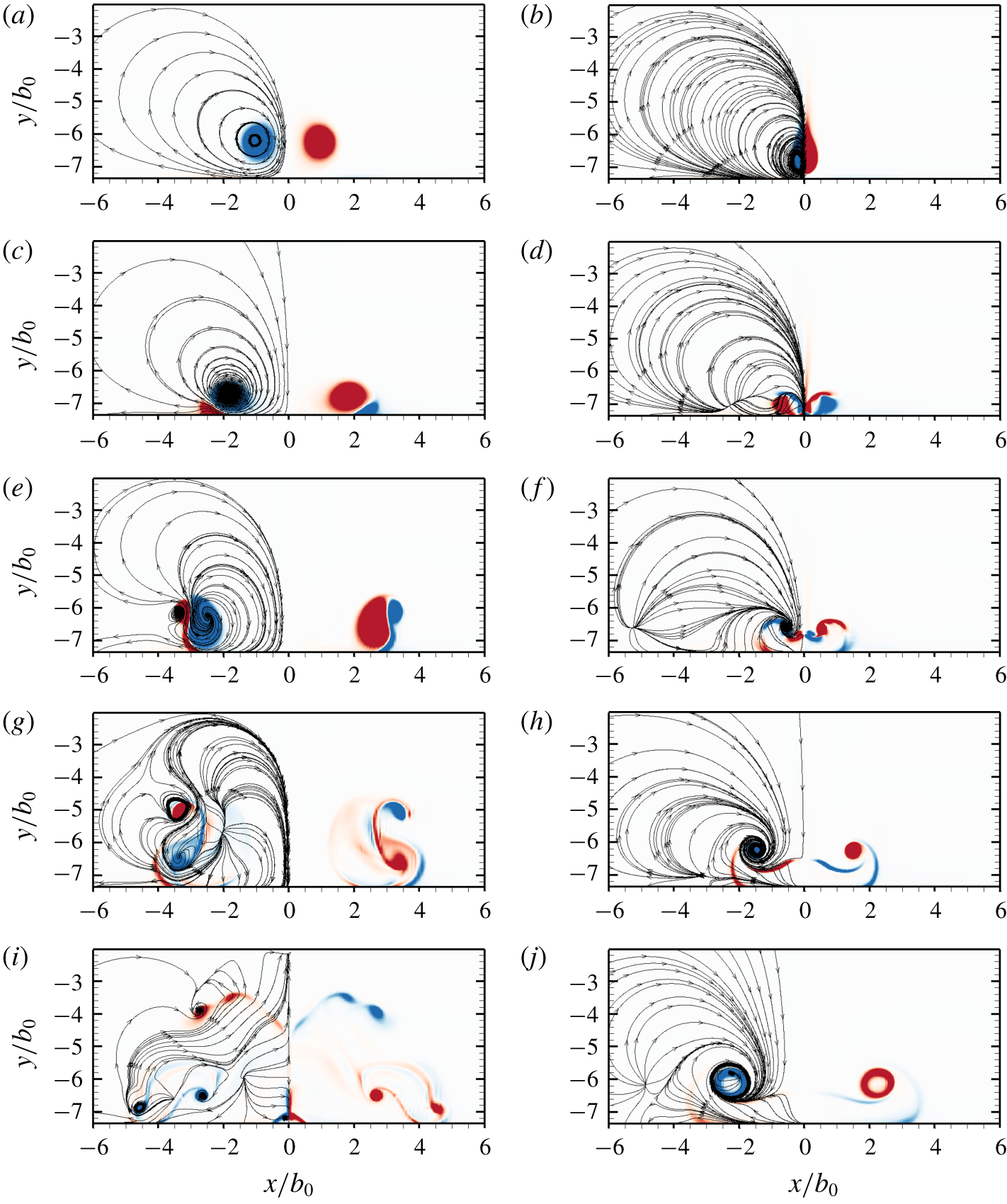
Figure 15 shows a comparison of the vorticity at the initial peak and trough of the instability. The vorticity contours at the peak of the Crow instability are reminiscent of the two-dimensional wall-bounded instability, where once the secondary vorticity separates from the boundary layer to form a discrete vortex (figure 15a), it closely orbits the primary vortex. Unlike the two-dimensional instability, however, at  $\unicode[STIX]{x1D70F}=3.98$ (figure 15c,d), the instantaneous streamlines of the secondary vorticity at both the peak and trough is oriented away from the primary vortices, and the formation of the characteristic tongue topology begins. The mechanism of tongue formation at the initial peak is weaker, and the separation between the primary and secondary vortex, although greater than the two-dimensional Crow instability, is small relative to the initial trough (figures 15e and 15f). The collapse of the primary vortex at the initial peak is first evident in figure 15(g), where the primary in-plane vorticity is no longer concentrated to a circular region, and both deforms and expands to a larger area.
The large vortex tongues are formed at the initial trough of the instability (figure 15d), and the peaks interact with the plane of symmetry well above the primary vortices (figure 15h). It is clear that vorticity with opposite sign belongs entirely to the primary vortex structure, and the tongues do not reconnect to form rings in the small-amplitude mode. Both primary and secondary vortex tongues are again observed to interact with the plane of symmetry (see figure 15i,j), with figures 15(e) through 15(j) further illustrating the generation of tertiary vortices at the wall.
The key observations of the numerical study of the small-amplitude mode can be summarised as follows:
(i) Four vortex tongues as opposed to two observed by Asselin & Williamson (Reference Asselin and Williamson2017) form.
(ii) The secondary vortex remains connected and does not form vertical vortex rings as observed by Asselin & Williamson (Reference Asselin and Williamson2017).
(iii) The vortex tongues interact at the symmetry plane to form loop-like structures prior to dissipation.
(iv) The rotation of the instability plane is a defining feature of the mode and plays a critical role in the dynamics.
(v) Strong axial pressure driven flow drives vortex breakdown, and plays an important role in the instability and evolution of the primary vortex. Even at small instability amplitudes, it is clear that the dynamics differs greatly as compared to the two-dimensional case.
3.3 Large-amplitude mode
At larger initial wall heights, the Crow instability evolves to larger amplitudes prior to interaction with the ground plane. Experimental visualisations suggested the formation of two horizontally oriented vortex rings which ‘rebound’ from the ground plane. The DNS does not support this conclusion, with the observation of the formation of a topologically complex vortical structure which wraps around the primary vortex. The study discussed here is at  $Re=2500$,
 $a_{0}/b_{0}=0.23$,
 $h_{0}/b_{0}=7.5$ and
 $A_{0}/b_{0}=0.01$ corresponding to an amplitude one vortex spacing above the ground plane of
 $A/b_{0}=0.4731$. This section is organised as follows; first, the evolution of the vortices is discussed, with the various features of the evolution isolated and presented; second, the pressure differential between peak and trough is related to the dynamics; and third, vorticity contours at select cross-sections are used to gain further insight into the flow evolution and to compare to both experimental visualisations and other modes of interaction.
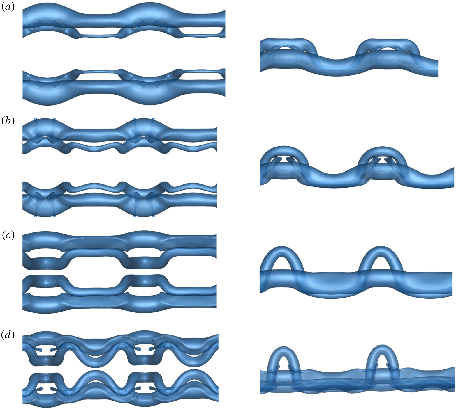
As the long-wave instability develops, the troughs of the instability move closer as the peaks move apart (see figures 16a and 17a). Viscous annihilation, prior to wall interaction, is locally enhanced at the trough of the instability. As a result of this primary–primary (PV1 and PV2) vortex interaction, locally higher pressure drives flow axially away from the trough to the peak of the instability. The rotation of the plane of instability, as observed in the small-amplitude mode, does not occur for the large-amplitude mode. The Crow amplitude continues to grow at  $\unicode[STIX]{x1D703}=45^{\circ }$ outside of the wall effect, and does not rotate near the wall. As such, the reversal of the peak and trough does not occur, and the trough is almost completely evacuated of vortical fluid (figures 16b and 17b). The instability interacts with the wall at a near
 $\unicode[STIX]{x1D703}=45^{\circ }$ angle, and strong secondary vorticity at the wall forms parallel to the primary pair, starting near the trough of the instability. As in the small-amplitude mode, the vorticity rolls up into a secondary vortex (SV1 and SV2) which induces a restoring force on the primary vortex pair, in the direction opposite to its radial expansion. The primary vortices undergo a ‘rebound’ effect due to the induced velocity of the secondary vorticity. Owing to the large curvature of the secondary vortex (seen clearly in figures 16b and 16c), the dynamics of the rebound is markedly different from both the two-dimensional Crow instability and the small-amplitude three-dimensional instability. As the primary vortices begin to interact with the ground plane and move apart from each other on a near hyperbolic trajectory, the formation of the secondary vorticity radially arrests the radial expansion of the primary vortices. The induced velocity causing the rebound effect is markedly stronger at the trough regions, resulting in enhanced bending at the troughs. The process of re-connection between the primary vortices begins but then ceases as the vortices move apart forming a vortex bridge (figure 16c). The primary vortex pair remains connected by the vortex bridge consisting of two equal strength counter rotating vortices per Crow instability wavelength (see figure 16d–f).
The evolution of the large-amplitude mode projected onto the  $x{-}z$ plane, here pictured for
 $Re=2500$,
 $a_{0}/b_{0}=0.23$ and
 $h_{0}/b_{0}=7.5$. The times for the snapshots are as follows: (a)
 $\unicode[STIX]{x1D70F}=7.96$; (b)
 $\unicode[STIX]{x1D70F}=9.55$; (c)
 $\unicode[STIX]{x1D70F}=11.14$; (d)
 $\unicode[STIX]{x1D70F}=12.73$; (e)
 $\unicode[STIX]{x1D70F}=15.91$; (f)
 $\unicode[STIX]{x1D70F}=16.71$. The labels PV and SV refer to the primary and secondary vortices respectively. The supplementary movie (movie 2 at https://doi.org/10.1017/jfm.2019.816) animates the evolution and is extremely helpful for visualisation.

The evolution of the large-amplitude mode projected onto the  $y{-}z$ plane, here pictured for
 $Re=2500$,
 $a_{0}/b_{0}=0.23$ and
 $h_{0}/b_{0}=7.5$. The times for the snapshots are as follows: (a)
 $\unicode[STIX]{x1D70F}=7.96$; (b)
 $\unicode[STIX]{x1D70F}=9.55$; (c)
 $\unicode[STIX]{x1D70F}=11.14$; (d)
 $\unicode[STIX]{x1D70F}=12.73$; (e)
 $\unicode[STIX]{x1D70F}=15.91$; (f)
 $\unicode[STIX]{x1D70F}=16.71$. See figure 16 for further information.

As the secondary vortices are advected about the primary vortices, they each bend and stretch inwards to form a horizontally oriented tongue (T1 and T2) around the now ‘collapsed’ primary vortex, as shown in figures 16(c) and 17(d). Two tongues form instead of the four of the small-amplitude mode as the instability plane does not rotate. The secondary vortex undergoes a connective process with the primary vortex, seen initially at the trough in figure 16(b). These do not re-connect to form horizontally oriented rings as previously suggested in the literature, but remain topologically complex vortex cores which wrap around the primary vortex. The tongues ‘rebound’ off the ground plane and rise well above the primary vortex pair (see figure 17d,e).
 $Q$-criterion isosurfaces of the various features in the evolution of the large-amplitude mode. (a) An
 $y{-}z$ view rotated about
 $z$ by
 $45^{\circ }$ of the isolated vortex tongue with pressure contours at large time steps. Vortex lines are shown in red to illustrate the complex connected topology. (b) Isometric view of the long-term evolution (
 $\unicode[STIX]{x1D70F}=34.93$) of the large amplitude mode with contours of the
 $\unicode[STIX]{x1D714}_{z}$ vorticity plotted. (c) Development of the primary vortex at
 $\unicode[STIX]{x1D70F}=13.52$ illustrating the inner tongue formation and the re-connective process to the secondary vortex with contours of the
 $\unicode[STIX]{x1D714}_{z}$ vorticity plotted. (d) Long-term evolution
 $\unicode[STIX]{x1D70F}=35.65$ of the primary vortex with contours of pressure, illustrating the resultant distortion. For contours of
 $\unicode[STIX]{x1D714}_{z}$, red indicates positive vorticity, and blue indicates negative vorticity. For contours of pressure, the contour levels range from blue to green to red from the minimum to maximum pressure at a given solution time.

Pressure differential of the vortex pair for the large amplitude mode at  $Re=2500$ and
 $a_{0}/b_{0}=0.23$ illustrating the axial flow evolution in the primary vortices. The lines represent pressure differentials between the following cross-sections: the dashed line (- -) between the peak and trough, the red line (——) between the peak and mid-plane and the blue line (——) between the mid-plane and trough. The supplementary movie (movie 2 at https://doi.org/10.1017/jfm.2019.816) animates the evolution and is extremely helpful for comparison to this figure.

Concurrent with the formation and rise of the horizontal vortex tongues, the primary vortex is bent inwards, and the point of re-connection between primary and secondary vortices both rotates and translates toward the centre of the collapsed vortex, shown in figure 16(b–d). The resultant reconnected vortex is stretched around the primary vortex, and at large times (see figure 16f), where the two re-connection regions are near one another, vorticity annihilation between the secondary vortices results in the formation of a highly non-planar tongue pictured in figure 18(a). The secondary vortex structures advect towards and interact with the plane of symmetry (see T1 and T2 in figures 16f and 17f), resulting in the radial expansion of the secondary tongues at the symmetry plane, alongside strong dissipation due to vorticity annihilation. The weaker vortex structures also dissipate, resulting in the large time evolution of the flow pictured in figure 18(b). The secondary structures at the plane of symmetry eventually dissipate, leaving behind both primary vortices now highly non-uniform after the wall interaction as shown in figure 18(d). Figure 19 illustrates the evolution through the lens of pressure and axial flow, clearly illustrating the strong axial flows away from the peak.
The  $z$ component of vorticity contoured onto cross-sections of the initial peak of the instability,
 $z=\unicode[STIX]{x1D706}/4$ (pictured in the left column) and the initial trough of the instability,
 $z=3\unicode[STIX]{x1D706}/4$ (pictured in the right column) for the large-amplitude mode at different times, here pictured for
 $Re=2500$,
 $h_{0}/b_{0}=5.0$ and
 $a_{0}/b_{0}=0.23$. Instantaneous streamlines are shown for half the domain and are symmetric about
 $x/b_{0}=0$. Red indicates positive vorticity, blue indicates negative vorticity. The times for the snapshots are as follows: (a,b)
 $\unicode[STIX]{x1D70F}=6.37$; (c,d)
 $\unicode[STIX]{x1D70F}=7.96$; (e,f)
 $\unicode[STIX]{x1D70F}=9.55$; (g,h)
 $\unicode[STIX]{x1D70F}=11.94$; (i,j)
 $\unicode[STIX]{x1D70F}=16.71$.

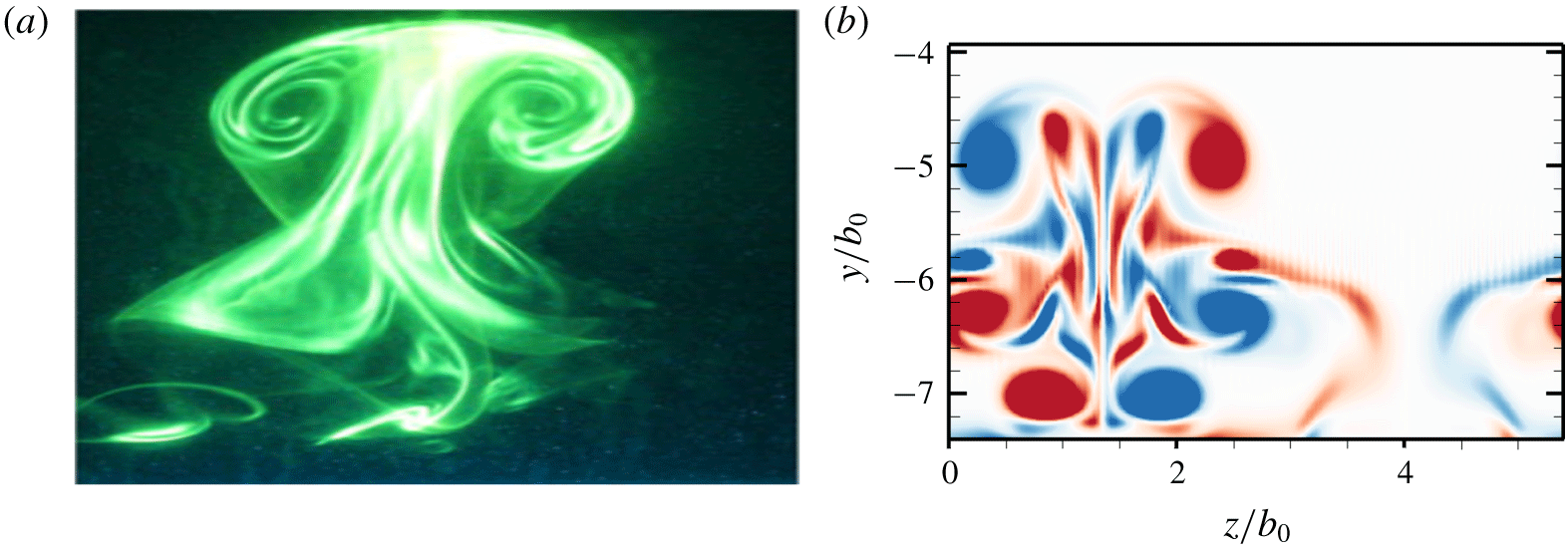
The ‘rebound’ of the secondary vortices in the large amplitude mode is illustrated and compared to experimental observations. (a) The large-amplitude mode experimentally illuminated by dye (Asselin & Williamson Reference Asselin and Williamson2017); (b)  $\unicode[STIX]{x1D714}_{x}$ contours of vorticity plotted on the
 $y{-}z$ plane corresponding to the centre of the primary vortex at
 $\unicode[STIX]{x1D70F}=11.94$. One wavelength of the large-amplitude mode for
 $Re=2500$,
 $a_{0}/b_{0}=0.23$ and
 $h_{0}/b_{0}=7.5$ is shown.

Analogous to the small-amplitude mode, vorticity contours at select cross-sections provide further insight into the flow evolution and provide clear comparison between the modes of interaction.
Vorticity contours at both peak and trough cross-sections, as well as in the  $y{-}z$ plane, are presented in figures 20 and 21, showing cross-sections of the complex flow evolution. In the plane of the peak of the instability, the secondary vortex separates from the ground plane (figure 20c,e) before rotating about the primary vortex and stretching outwards (figure 20g). The formation of the large secondary loops (figure 20g,i) is evident. In the plane of the trough of the instability, the enhanced pressure drives the flow axially away from the trough, with much of the fluid driven away from the region (see figure 20d,f). After the rebound and during the pressure gradient reversal, fluid is driven back to the troughs (figure 20h). The strong axial flow results in the vortices entraining irrotational flow, and as the characteristic vortex core size increases under viscous effects, a hollow vortex forms (see figure 20j), also observed in experiment (Asselin & Williamson Reference Asselin and Williamson2017). After the ‘rebound’ of the secondary vorticity, the secondary vortex tongue rises well above the primary pair to form the characteristic T-shaped vortical structures observed experimentally (figure 21a), with the additional complexities of the tongue visible in the DNS (figure 21b).
To summarise, the key observations of the DNS study of the large-amplitude mode are as follows:
(i) The instability plane does not rotate unlike the small-amplitude mode, distinguishing the two modes of interaction.
(ii) The formation of only two vortex tongues, as opposed to four in the case of the small-amplitude mode, is observed at the trough of the instability.
(iii) Two complex connected vortical tongues form and wrap around the primary vortex. These are not horizontally oriented vortex rings as observed by Asselin & Williamson (Reference Asselin and Williamson2017) based on experimental visualisation.
(iv) Strong axial flow away from the trough, and the formation of the secondary tongues, strongly influences the primary vortex evolution, and the vortex becomes heavily distorted at large times.
3.4 Large ring mode
The dynamics and evolution of the wall-bounded interaction and instability undergoes a significant change if the primary vortex pair forms rings prior to wall interaction. This mode of interaction presents a difficulty in that the topology of the rings in the unbounded instability varies with time (Leweke & Williamson Reference Leweke and Williamson2011). The vortex pair first forms elliptic rings oriented in the  $x$-direction, followed by elliptic rings in the axial direction and ultimately undergoes a second reconnection. As the flow physics of the wall-bounded instability is sensitive to the regions of the vortex pair closest to the wall, the dynamics of the large ring mode varies as a function of initial vortex height
 $h_{0}/b_{0}$. The results presented in this section are shown for
 $h_{0}/b_{0}=10.0$, consistent with the initial vortex configuration after reconnection as observed experimentally by Leweke & Williamson (Reference Leweke and Williamson2011). Despite the anticipated complexity of the resultant ring–ring–wall interaction, the flow exhibits remarkable symmetries with strong parallels to the other modes of interaction.
This subsection is organised as follows. First the evolution of the vortical structures is discussed. Second, the pressure and vorticity at key cross-sections is visualised and connected to the dynamics.
Above a critical height above the ground plane, where the primary vortex pair (PV1 and PV2) evolves outside of the wall effect, the vortex pair evolves identically to the unbounded instability, with the formation of non-planar elliptic rings (PR) visible in figures 22(a) and 23(a). In this initial configuration, the region of the ring closest to the initial trough of the instability interacts with the ground plane first (see figure 23b). The relatively large initial curvature of the non-planar ring, visible in figure 23(a), results in the local formation of boundary layer vorticity, which, analogous to the other modes, rolls up to form a vortex and induces a velocity on the primary ring resulting in the ‘rebound’ effect. The rebound is locally stronger in regions of the ring near the wall, and the ring evolves into a near planar configuration, as shown in figure 23(c). The evolution in the pressure differential shows the axial flow development primarily due to the formation of rings in figure 24. Simultaneously, the secondary vorticity rolls up and separates from the ground forming a secondary ring (SR in figures 22c and 23c). The primary rings both ‘rebound’ and expand radially outwards until arrested by the formation of the secondary rings (see figures 22d and 23d). Upon ‘expansion’, the primary vortex rings interact at the initial trough of the instability, and the characteristic vortex tongues (T1 through T6) begin to form as seen in figures 22(e) and 23(e).
The evolution of the large ring mode projected onto the  $x{-}z$ plane, here pictured for
 $Re=2500$,
 $a_{0}/b_{0}=0.23$ and
 $h_{0}/b_{0}=10$. The configuration of the vortex pair prior to wall interaction is representative of the first configuration of the long-wave instability after the initial re-connective process. Contours of pressure are plotted on the vortex isosurfaces. The contour levels are from blue to red between minimum and maximum pressure of the entire evolution respectively. The times for the snapshots are as follows: (a)
 $\unicode[STIX]{x1D70F}=7.96$; (b)
 $\unicode[STIX]{x1D70F}=8.76$; (c)
 $\unicode[STIX]{x1D70F}=11.14$; (d)
 $\unicode[STIX]{x1D70F}=11.94$; (e)
 $\unicode[STIX]{x1D70F}=13.53$; (f)
 $\unicode[STIX]{x1D70F}=14.33$; (g)
 $\unicode[STIX]{x1D70F}=15.12$; (h)
 $\unicode[STIX]{x1D70F}=15.92$; (i)
 $\unicode[STIX]{x1D70F}=17.52$; (j)
 $\unicode[STIX]{x1D70F}=19.10$; (k)
 $\unicode[STIX]{x1D70F}=20.69$; (l)
 $\unicode[STIX]{x1D70F}=23.87$. The labels PV, PR and SR refer to the primary vortices, primary vortex ring and the secondary vortex ring respectively; the labels T1–T6 refer to the secondary vortex tongues; the labels L1–L2 refer to the ‘loop-like’ structures and the labels PT1–PT2 refer to the primary vortex tongue structures identified and discussed in the text. The supplementary movie (movie 3 at https://doi.org/10.1017/jfm.2019.816) animates the evolution and is extremely helpful for visualisation.

The evolution of the large ring mode projected onto the  $y{-}z$ plane, here pictured for
 $Re=2500$,
 $a_{0}/b_{0}=0.23$ and
 $h_{0}/b_{0}=10$. The configuration of the vortex pair prior to wall interaction is representative of the first configuration of the long-wave instability after the initial re-connective process. Contours of pressure are plotted on the vortex isosurfaces. The contour levels are from blue to red between minimum and maximum pressure of the entire evolution respectively. The times for the snapshots are as follows: (a)
 $\unicode[STIX]{x1D70F}=7.96$; (b)
 $\unicode[STIX]{x1D70F}=8.76$; (c)
 $\unicode[STIX]{x1D70F}=11.14$; (d)
 $\unicode[STIX]{x1D70F}=11.94$; (e)
 $\unicode[STIX]{x1D70F}=13.53$; (f)
 $\unicode[STIX]{x1D70F}=14.33$; (g)
 $\unicode[STIX]{x1D70F}=15.12$; (h)
 $\unicode[STIX]{x1D70F}=15.92$; (i)
 $\unicode[STIX]{x1D70F}=17.52$; (j)
 $\unicode[STIX]{x1D70F}=19.10$; (k)
 $\unicode[STIX]{x1D70F}=20.69$; (l)
 $\unicode[STIX]{x1D70F}=23.87$. See figure 22 for further information.

For the studied parameters, six vortex tongues form per instability wavelength (see figures 22f and 23f), which rotate about the primary vortex prior to advection towards the symmetry plane as in figures 22(h) and 23(h). The formation of tongues corresponds to three local peaks and troughs of the instability. Two of the local extrema originate from the trough regions of the Crow instability during reconnection (forming T1–T4). The third extremum is a result of the vortical structure due to the bridging between the vortex rings (forming T5 and T6). The four vortex tongues (T1–T4) formed at the ‘corners’ of the vortex rings observed in figure 22(e) are identical under symmetric reflection and rotation, but differ in structure from the other two vortex tongues (T5–T6) at the mid-plane of the ring. After formation, the lower sections of the tongues are wrapped underneath the primary vortex. The secondary vortex ring remains entirely connected by  $\unicode[STIX]{x1D70F}=28.65$ shown in figures 22(f) and 23(f). Unlike the small amplitude mode, however, the rebound effect for the studied parameter does not lift the primary ring far from the ground plane, resulting in significant vorticity annihilation with the wall-bounded vorticity. A process of re-connection hence occurs between the tongues and the primary ring to form complex non-planar vortex loops similar to the large-amplitude mode illustrated in figures 22(i) and 23(i). The tongues interact at the plane of symmetry (see figures 22j and 23j), and undergo rapid radial expansion. Both the primary and secondary vortices proceed to strongly dissipate, ultimately resulting in the long term evolution pictured in figures 22(l) and 23(l).
Tertiary vortices (TV) form and are clearly seen in figure 22(f), but for the parameters of this study, the tertiary vortex is not strong enough to arrest the radial expansion, and the primary vortices begin to interact with one another. The interaction between primary vortex rings (PR–PR) is similar to the interaction of secondary tongues at the symmetry planes. These regions of the primary vortex rise above the ground plane due to mutual interaction, and form wide tongue-like structures (PT1 and PT2) evidenced in figures 22(h–j) and 23(h–j). As the primary rings continue to radially expand, the peaks of the primary tongues undergo a re-connection process, resulting in complex hairpin-like structures observed in figures 22(k) and 23(k).
Pressure differential of the vortex pair for the large ring mode at  $Re=2500$ and
 $a_{0}/b_{0}=0.23$ illustrating the axial flow evolution in the primary vortices. The lines represent pressure differentials between the following cross-sections: the dashed line (- -) between the peak and trough, the red line (——) between the peak and mid-plane and the blue line (——) between the mid-plane and trough. The supplementary movie (movie 3 at https://doi.org/10.1017/jfm.2019.816) animates the evolution and is extremely helpful for comparison to this figure.

The physics behind the bending and stretching of the vortex cores about the circumferential axis and the formation of vortex tongues is comparable to oblique ring/wall interaction (cf. Lim (Reference Lim1989), Verzicco & Orlandi (Reference Verzicco and Orlandi1994), Swearingen et al. (Reference Swearingen, Crouch and Handler1995) and Cheng et al. (Reference Cheng, Lou and Luo2010)). In particular, the observations and physical explanations of Verzicco & Orlandi (Reference Verzicco and Orlandi1994) are highly analogous to those of the present work.
Vorticity contours at select planes provide additional insight into the flow physics and allow for a direct comparison to the other modes of interaction. The vorticity contours at the peak cross-section illustrates the boundary layer vorticity (figure 25a) resulting in the formation of secondary (figure 25c), tertiary (figure 25d) and even quaternary vortices (figure 25f), which separate from the boundary layer and rotate about the primary ring. In the large ring mode, where the rebound effect is not highly pronounced, stronger vortices continue to form due to the ground as compared to the small- and large-amplitude modes. The secondary vortices hence ‘tightly’ wrap around the primary vortex, resulting in inner and outer counter rotating sections (figure 25h). The vorticity at the initial trough shows the initial vortex bridge between the primary ring (figure 25b–e), with little boundary layer generated vorticity. At larger time steps, due to the ground plane interaction, the primary rings interact with each other at the trough, and the vortices rise due to the induced velocity, as evidenced by figure 25(g–j).
The  $z$ component of vorticity contoured onto cross-sections of the initial peak of the instability,
 $z=\unicode[STIX]{x1D706}/4$ (pictured in the left column) and the initial trough of the instability,
 $z=3\unicode[STIX]{x1D706}/4$ (pictured in the right column) for the large ring mode at different times, here pictured for
 $Re=2500$,
 $h_{0}/b_{0}=10.0$ and
 $a_{0}/b_{0}=0.23$. Instantaneous streamlines are shown for half the domain and are symmetric about
 $x/b_{0}=0$. Red indicates positive vorticity, blue indicates negative vorticity. The times for the snapshots are as follows: (a,b)
 $\unicode[STIX]{x1D70F}=11.14$; (c,d)
 $\unicode[STIX]{x1D70F}=11.94$; (e,f)
 $\unicode[STIX]{x1D70F}=13.53$; (g,h)
 $\unicode[STIX]{x1D70F}=15.12$; (i,j)
 $\unicode[STIX]{x1D70F}=16.71$.

The key observations of the DNS study of the large ring mode in its first formation are summarised as follows:
(i) A connected secondary vortex ring forms upon wall interaction.
(ii) The secondary vortex ring remains connected and forms six secondary vortex tongues per Crow wavelength.
(iii) The ‘rebound’ effect is significantly less pronounced as compared to the other modes of interaction.
(iv) Ring–ring interaction plays an important role in the long-term dynamics.
(v) Unlike the other modes of interaction where secondary vorticity dissipates leaving the primary vortices behind, the primary vortex ring dissipates at close to the same time scale as the secondary vortex tongues.
4 Reynolds number and core size effects
The numerical study was conducted at various Reynolds numbers and three core sizes to investigate the influence of the Reynolds number and core size on the flow physics. The comparison presented here does not seek to investigate the entire parameter space but rather to show that the modes and observed instability evolution are not specific to the choice of parameters presented in the results.
A study at a low Reynolds number, nominally for  $Re=1000$ and
 $a_{0}/b_{0}=0.4$, was conducted. It was found that at these parameters, the growth rate of the instability was small, and the necessary initial instability amplitude
 $A/b_{0}$ was rather large (
 ${\sim}0.1$) to ensure the development of the appropriate modes upon wall interaction. The initial flow configuration governing the formation of the various vortex tongues and dictating the flow evolution was observed, but the system was found to dissipate under viscous effects prior to the formation of tongues or rings.
 $Q$-criterion vortex visualisation of the instability for the small-amplitude mode for variation in core size and Reynolds numbers. Both the
 $x{-}z$ (pictured left) and
 $y{-}z$ (pictured right) views are shown. (a)
 $Re=1500$ at
 $\unicode[STIX]{x1D70F}=11.14$ with
 $h/b_{0}=3.5$ and
 $a_{0}/b_{0}=0.4$. (b)
 $Re=2000$ at
 $\unicode[STIX]{x1D70F}=11.14$ with
 $h/b_{0}=3.5$ and
 $a_{0}/b_{0}=0.4$. (c)
 $Re=2500$ at
 $\unicode[STIX]{x1D70F}=15.92$ with
 $h/b_{0}=5.0$ and
 $a_{0}/b_{0}=0.4$, which correspond to the parameters quoted in Asselin & Williamson (Reference Asselin and Williamson2017). (d)
 $Re=2500$ at
 $\unicode[STIX]{x1D70F}=12.0$ with
 $h/b_{0}=5.0$ and
 $a_{0}/b_{0}=0.3$, which correspond closely to the parameters defining the least squares fit of the initial velocity distribution shown in Asselin & Williamson (Reference Asselin and Williamson2017).

Figure 26 gives an indication of the effect of a different Reynolds number and core size on the formation of vortex tongues by looking at the small-amplitude mode. At an initial starting height of  $h_{0}/b_{0}=5.0$, the low Reynolds number cases strongly dissipate prior to wall interaction. Contrariwise, at an initial starting height of
 $h_{0}/b_{0}=3.5$, the perturbation amplitude of the large Reynolds number case upon wall interaction is not large enough for the pronounced three-dimensional features to develop, and the interaction is predominantly two-dimensional. At these smaller Reynolds numbers, the vortex tongue is either almost entirely dissipated (figure 26a) or significantly less pronounced (figure 26b) prior to vertical orientation. Very small peak tongue structures form at larger times for the
 $Re=2000$ and
 $Re=2500$ cases, but their formation is greatly inhibited as compared to the smaller core size study in § 3. For the tongues to form, the Reynolds number needs to be high enough such that the vortex loop separates from the boundary layer vorticity. At the large Reynolds number of
 $Re=2500$ and
 $h_{0}/b_{0}=5.0$, which corresponds to the parameters quoted in Asselin & Williamson (Reference Asselin and Williamson2017) (
 $Re_{a}=1000$,
 $a/b_{0}=0.4$), two distinct tongues form per long wavelength at the trough of the instability and the secondary vortex remains connected (figure 26c). The increase in core size inhibits the growth of the additional tongues. The two vortex tongues, however, vertically orient at a later time as compared to the experimental results. At a smaller core size of
 $a/b_{0}=0.3$, which corresponds closely to the least squares fit of the superposition of two Gaussian vortices to the experimental data plotted in Asselin & Williamson (Reference Asselin and Williamson2017) (
 $Re_{a}=750$,
 $a/b_{0}=0.3$), the tongues vertically orient at a similar time as compared to the experiments (see figure 26d). At this smaller core size, however, the formation of four vortex tongues, as opposed to the two observed by experiment, is clearly visible.
A core size of  $a_{0}/b_{0}=0.23$ is hence chosen for the primary study as an analogue to the experiments of Leweke & Williamson (Reference Leweke and Williamson1998); the smaller core size allows for better visualisation of the various features of the flow, particularly the additional vortex tongues, and still clearly resolves all three modes of interaction observed by Asselin & Williamson (Reference Asselin and Williamson2017). The primary distinctions between the results for different Reynolds numbers are: the growth rate of the wall-bounded instability, for which the initial amplitude needs to be varied to ensure the appropriate amplitude of the instability near the wall; the size of the tongues formed, due to stronger secondary vortex formation; and the dissipative effects, which result in less coherent structures at lower Reynolds numbers. Provided the Reynolds number is large enough such that the vortical structures do not dissipate prior to the formation of coherent vortices, it appears that for Reynolds numbers in the order of
 $Re\sim 10^{3}$, the macroscopic features of the modes observed are independent of the parameters chosen.
5 Conclusions
A study of the three-dimensional long-wavelength stability of a counter-rotating vortex pair in the presence of a wall was conducted. The DNS provided an understanding of the entire evolution of the three modes observed by Asselin & Williamson (Reference Asselin and Williamson2017), including both the initial development phase and the nonlinear interaction phase. The numerical simulations do not confirm the conjecture of Asselin & Williamson (Reference Asselin and Williamson2017) that secondary vertical or horizontal rings are formed, but rather reveal that the fine-scale dynamics is more surely dominated by ‘tongues’ and ‘loops’ that do not reconnect into vortex rings. These three modes of wall-bounded interaction, hence renamed the ‘small-amplitude mode’, the ‘large-amplitude mode’ and the ‘large ring mode’, differ based on the development of the Crow instability prior to strong wall interaction, characterised by the amplitude of the instability one initial vortex spacing above the wall  $A/b_{0}$.
In all cases, the wall significantly altered the development of the long-wavelength instability, with the resultant flow field highly three-dimensional. The formation of characteristic hairpin-like vortex tongues is observed for all modes, which drastically alters the evolution of the primary vortex pair. Both the primary and secondary structures ‘rebound’ off the wall, and the resultant evolution is markedly different from both the unbounded instability and the two-dimensional bounded instability.
For the small-amplitude mode, recovered in this study for  $A/b_{0}=0.1371$, the resultant formation of secondary vortex tongues interact with one another at the mid plane of the primary vortex pair. The DNS uncovers the primary mechanism for this mode, namely the rotation of the plane of instability to a near
 $0^{\circ }$ orientation at the wall. The wall also acts to inhibit the growth of the instability via the formation of boundary layer vorticity. The large-amplitude mode differs from the small-amplitude mode in that the difference in viscous interaction from peak to trough at the wall is significantly larger. The fundamental reason for this is that the plane containing the instability does not rotate much from
 $45^{\circ }$ prior to strong viscous wall interaction. Finally, the large ring mode is characterised by the formation of rings prior to wall interaction. The topology of the rings prior to wall interaction is a strong function of the time outside of ground effect (cf. Leweke & Williamson Reference Leweke and Williamson2011), and the resultant wall-bounded evolution hence varies with the initial vortex starting height. Specifically, the case of the initial ring topology evolution due to the cooperative instability, namely the formation of non-planar spanwise oriented elliptic rings is analysed, and striking similarities are found between the other modes of interaction.
The mechanism governing the formation of the vortex tongue structures is for all modes related to the difference in distance from the wall to the perturbed primary vortex, which varies as a function of the axial coordinate. Sections of the primary vortex closest to the wall undergo a local increase in vorticity annihilation, resulting in a local increase in pressure driving the fluid axially away from the trough regions. This results in magnified stretching and rotation of these localised regions of the separated secondary vortex, resulting in the formation of secondary loops.
For the small-amplitude mode, the secondary vortex remains connected until dissipative effects take hold, and is even observed to form a second set of smaller tongues after a full rotation about the primary vortex. Both sets of tongues consist of four tongues per wavelength of the Crow instability. Of the first set of tongues which form between the primary vortices, two large and two small tongues form per wavelength. These tongues rebound and interact with the plane of symmetry well above the primary vortex pair, and the large tongues expand outwards to form large planar ring-like structures. The long-term evolution of the flow sees a distorted primary vortex pair, influenced by the evolution of the secondary tongues, with the four vortex tongues dissipating by the action of viscosity at the peak and trough axial cross-sections of the primary pair.
The evolution of the large-amplitude mode shows the disconnection of the secondary vortex, with a re-connective process resulting in the formation of highly non-planar connected vortical structures that are stretched and rotated around the primary vortex, of which there are two per Crow wavelength. The structures rebound and the tops of the structures rise well above the primary vortex pair. A series of complex re-connective processes characterises the flow evolution. A primary vortex tongue forms at the initial peak of the primary vortex, and strong axial flow from trough to peak results in a hollow vortex. At large times, the secondary vortex structures interact with the mid-plane to form large planar ring-like structures similar to those of the small-amplitude mode prior to dissipation and the primary vortex pair remains highly distorted.
At initial amplitudes large enough such that the primary vortex pair develops into a periodic series of rings under the long-wave cooperative instability, the wall interaction is a strong function of the initial height at which the vortices are generated. For the first configuration of the vortex rings after the initial re-connection, the rings radially expand upon wall interaction and six secondary vortex tongues are formed per Crow wavelength. The rings are initially non-planar, but ‘flatten’ out upon wall interaction to form ellipses with a spanwise major axis. The tongues ‘rebound’ and undergo re-connective processes similar to the large-amplitude mode, although the ‘rebound’ effect is not as pronounced. The loops of the tongues approach each other and interact in the mid-plane and expand outwards prior to dissipation. The primary vortex ring expansion is arrested by primary ring–ring interaction, resulting in the growth and formation of hairpin-like structures between the primary rings. Unlike the other two modes of interaction, the primary vortex rings dissipate within the same order of time scale as the secondary vorticity; the long-term evolution of the flow is hence observed to be gradual dissipation of the complex structures under the influence of vorticity diffusion.
The practical application of this research, alongside the similarities between the flow evolution of this study and other wall-bounded flow configurations, lends itself to a great deal of potential further interest. It is clear that physical controls to attempt to accelerate the growth rate of the Crow instability will need to consider the critical height at which the vortices are formed above the ground. Furthermore, validating the flow evolution for larger Reynolds numbers, both active and passive control of the growth of the wall-bounded instability, and investigations into the evolution of the large ring mode at different starting heights could extend this work to provide a detailed understanding of the physics underlying this fundamental flow configuration.
Acknowledgements
This work was supported by resources provided by the Pawsey Supercomputing Centre and the National Computational Infrastructure (NCI), with funding from the Australian Government and the Government of Western Australia for computing time available through Merit Project Grants n67 and d71.
Supplementary movies
Supplementary movies are available at https://doi.org/10.1017/jfm.2019.816.