2.1. Eulerian approach

We consider a Cartesian coordinate system with x, y the horizontal plane, z the vertical, and t time. The fundamental equation states that date of deposition A is a quantity that is conserved with time:

where d/dt is the full (total) time derivative. In an Eulerian frame, this equation can be rewritten with a partial (local) time derivative as:

where v_x, v_y, v_z are components of the three-dimensional velocity field. Boundary conditions are A(x, y, z = H + h, t) = t at the surface, with H ice thickness and h bed elevation. For an ice sheet frozen to the bottom, the date of deposition is undefined at the base (or physically equal to the time the first permanent ice cover settled at that particular location). In the case of basal melting, a flux boundary condition can be set at the base as follows:

where B is the basal melting rate (m a–₁), positive in the case of basal melting. In all runs discussed in this paper, we use second-order upwinding for all the advection terms. Since we only consider cases with basal melting, implying strict downward motion perpendicular to the ice layers, the basal boundary condition on A actually stands on its own and is never invoked to compute the date of deposition elsewhere. This prevents an arbitrary choice of basal ice age from polluting the solution at another location in the ice sheet. The case with negative B (basal freeze-on) cannot be handled with Equation (3) and is excluded from the analysis in this paper.

2.2. Lagrangian approach

In a Lagrangian frame which follows the particles, Equation (1) can be discretized in a straightforward way without any artificial diffusion. The approach consists of integration of a vector evolution equation:

where X(t) is the position vector of the ice particle and V(x, y, z, t) is the velocity field in the ice sheet. The initial condition for Equation (4) states that the trajectory of an ice particle deposited at the surface starts at time t₀ = A at the free surface H + h:

A trajectory ends when a particle crosses an arbitrary conventional bottom (we use 99% of relative depth) or leaves the ice sheet through its lateral margins.

The general problem in the Lagrangian approach consists of proper numerical interpolation of the velocity field. If piecewise linear interpolation is used, the velocity field is computed as a weighted sum of the field values in the surrounding gridpoints (four in two-dimensional space, eight in three-dimensional space). Cubic-spline interpolation requires knowledge of the velocity values in all or a subset of the model domain (Reference Press, Teukolsky, Vetterling and FlanneryPress and others, 1992).

3.1. Design of the standard experiment

We consider a two-dimensional ice sheet on a flat bedrock at z = 0 for which the surface profile can be given as:

where

This is the well-known Nye–Vialov solution (Reference PatersonPaterson, 1994), in which H is ice thickness (m), equated here to surface elevation, H₀ is the height of the ice sheet at the divide (m), L is the half-width of the profile (10₆ m), A is the rate factor of the flow law (10_–16 Pa–₃ a–₁), n is the flow-law exponent (taken to be 3), p is ice density (910 kg m–₃), g is acceleration of gravity (9.81 m s–₂) and M is the mass balance (m a–₁). With a typical value of M = 0.1 ma–₁, corresponding to a large polar ice sheet, we obtain a value for H₀ of 3598.4 m (see Table 1).

Table 1.

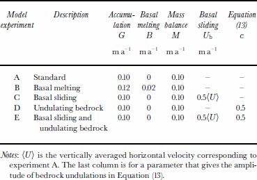
Parameter values for the various schematic tests in a two-dimensional plane

The horizontal velocity field as a function of depth can be derived along the flowline from Equations (6) and (7) to yield the following expression:

For the vertical velocity v_z a simple linear expression is used. This expression is not consistent with v_x as provided by Equation (8) but is used for simplicity because it allows for a straightforward analytical comparison at the divide:

Equations (6–9) entirely define a well-circumscribed problem for the purpose of comparing the dating methods. In practice, we use a dimensionless vertical coordinate scaled to ice thickness, and transform Equations (8) and (9) to this new system. Both the Lagrangian and Eulerian calculations take place directly in the transformed system.

The domain of the ice sheet given by Equations (6) and (7) is discretized by 101 6 101 gridpoints, equally spaced in dimensionless space. The experiments run for 500 kyr with a time-step of 1 year. Since the ice sheet is symmetrical with respect to the ice divide, we consider only the righthand domain, which consists of horizontal gridpoints 51–101. The Lagrangian method uses cubic-spline interpolation for the position integration. The results are shown in Figure 1. They are only valid for the upper 99% of ice thickness and between the divide and x = 980 km, because both boundaries are singular for one or both of the methods.

Fig. 1.

Results for the standard model run with flat bedrock, no basal melting and no basal sliding (experiment A). The streamlines are a direct output of the Lagrangian method and coincide with particle paths for a stationary state. The lower panels show the calculated dates of deposition from the Lagrangian and Eulerian methods, as well as their relative difference. Results are shown in the square that arises from the dimensionless vertical coordinate scaled to ice thickness.

In steady state, particle trajectories are equivalent to streamlines. These are shown in the top panel of Figure 1. Only 6 tracers out of 51 reach a relative depth of 99 %, while the others finish at the margin. This immediately demonstrates a basic problem with the Lagrangian method: in the deeper layers of the sheet, it yields less information than the Eulerian method, leading to an inherent loss of detail with depth. In our comparison, we solve this problem by launching 45 additional tracers between gridpoints 51 and 56, giving a density of 51 markers at 99 % depth, comparable to the Eulerian method. For clarity, however, these are not shown on the streamline plot.

On the scale of the plots, the two dating methods are almost indistinguishable. We therefore define a relative difference on date of deposition (“Eulerian error”) as follows:

where A_E is Eulerian date and A_L Lagrangian date. Negative relative differences indicate that the Lagrangian ice is older (i.e. the date of deposition is more negative) than the Eulerian ice for the same position. The relative difference between the two methods is very small (< 0.1 %) for most of the ice sheet, except at the model boundaries. The probable reasons for these differences are discussed in section 3.4 further below.

3.2. Comparison with an analytical solution at the divide

For the simple stationary case of no bottom melting, no horizontal advection, and constant vertical strain rate, a simple logarithmic expression for the date-of-deposition profile with depth can be derived, corresponding to our standard experiment at the divide:

where G is the surface accumulation rate, here equal to the mass balance M. This analytical derivation is due to Reference NyeNye (1963) and Reference HaefeliHaefeli (1963), and is known as the Nye–Haefeli time-scale.

We compare the analytical result at the divide with the numerical solution of the standard experiment A. In this case, the relative error of the numerical method is defined as:

where A_num is the date of deposition computed by either numerical method (Eulerian or Lagrangian), and A_an is given by Equation (11). The result is displayed in Figure 2. Clearly, the Lagrangian method produces less error, as is evident from the logarithmic scale required to show the relative errors. All along the vertical, the Lagrangian method slightly underestimates the date of deposition (i.e. produces an older date) but with a relative error always below 0.1% and often as good as 0.001 %. This error depends on the time-step and the grid size and is due to the accumulation of errors during the subsequent position interpolations of the ice particle travelling downwards. Relative to the date, this error becomes smaller the smaller the vertical velocity becomes nearer to the bottom. The error on the Eulerian calculations is also acceptably small, but has a different profile with depth. Except for the upper two vertical gridpoints, where second-to order upwinding cannot be used and a two-point upwinding scheme is only accurate to first order, the relative error is always < 0.1 % down to a relative depth of approximately 93%. For most of this part, E_num is negative, that is, the Eulerian date is more recent than the analytical solution, but E_num changes sign at 8 4% depth, when it becomes positive. Near to the bottom, the Eulerian error increases rather abruptly to a substantial level of several per cent. This originates from an inability of the numerical scheme to produce a precise result close to the lower boundary. There, the accuracy of the finite-difference scheme changes from second to first order, and gradients also become very large.

Fig. 2.

The error on date of deposition for both methods relative the analytical solution at the ice divide. The upper logarithmic axis is for the full line (Lagrangian), and the lower linear axis refers to the stippled line (Eulerian).

Notes: (U) is the vertically averaged horizontal velocity corresponding to experiment A. The last column is for a parameter that gives the amplitude of bedrock undulations in Equation (13).

3.3. Design of additional schematic tests

To test more challenging conditions more like real world-conditions, we modified the standard model set-up to investigate the effects of basal sliding, basal melting and an undulating bedrock. The modifications to the standard model are listed in Table 1. I n all of the additional experiments, the requirement was that the vertically integrated ice flux along the flowline was identical to that in the standard model. Also the surface profile was retained from the standard experiment. Although these additional tests violate basic principles underlying the Nye–Vialov solution, this is unproblematic as long as identical velocity and ice-thickness fields are used to compare the two dating methods. The basic design of the additional four experiments can be derived from the first column of streamline plots in Figure 3.

Fig. 3.

Results for the additional tests performed for a schematic two-dimensional stationary ice sheet showing streamlines, Lagrangian date and the relative difference between Lagrangian and Eulerian dates of deposition. The bold letters in the upper right corner refer to the specific experiment: B, basal melting; C, basal sliding; D, undulating bedrock; E, undulating bedrock and basal sliding (cf. Table 1 and the text for more details).

To meet the requirement of flux conservation, the basal melting experiment (experiment B) has to increase the surface accumulation by the same amount as the basal melting rate of B = 0.02 m a– ^₁ . The major effect of this modification is a non-zero vertical velocity at the base, resulting in more recent ice in the basal layers as compared to the standard experiment. By contrast, the introduction of basal sliding (experiment C) causes a flattening of the trajectories to resemble hyperbolas such that only the tracer starting at the divide reaches a depth of 99%, whereas the other tracers leave at the margin at x = 980 km. In this case, a 50–50 partitioning was put forward between horizontal movement due to deformation and due to basal sliding. To investigate the effect of a non-flat bed, an undulating bedrock profile (experiment D) was obtained as follows:

where c is a constant between 0 and 1 that gives the amplitude of the waves as a fraction of ice thickness H(x) in the standard experiment. To preserve the flux, the horizontal velocities are now scaled to the difference between the surface profile of the standard experiment and the revised bed elevation. Particles now follow an undulating pattern, with higher speeds over thinner ice and lower speeds over thicker ice, compared to the standard experiment. Finally, experiment E combines both an undulating bedrock and basal sliding.

3.4. Diversity in ice-age patterns produced by the two dating methods

From close inspection of Figures 1and 3 a number of general inferences can be drawn. The overriding conclusion is that the difference between the Lagrangian and Eulerian methods is very small. In general, the relative difference does not exceed 0.5% for most of the ice sheet. Larger relative differences only occur at the top and basal boundaries, and near to the lateral margin. This pattern is qualitatively similar for all schematic experiments. The reason for these systematic differences originates from the different methods and different sources of numerical errors. We cannot assess which method is closer to perfection, since no exact solution exists except at the divide. Nevertheless, the relative comparisons permit some conclusions.

It is reasonable to assume that the difference between the two methods near to the base and at the top is due to imperfections in the Eulerian scheme, since that is what the divide comparison brought to light. However, near the lateral margin (righthand margin of Fig. 4) the difference could also be attributed to the Lagrangian scheme due to the cumulative nature of its errors. In the Lagrangian approach, errors are proportional to travel time and to the velocity magnitude. Therefore the largest error will be at the end of the trajectory of a particle at the margin, where both quantities are largest.

Fig. 4.

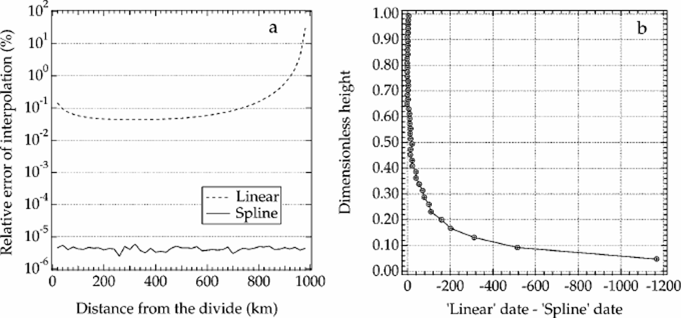
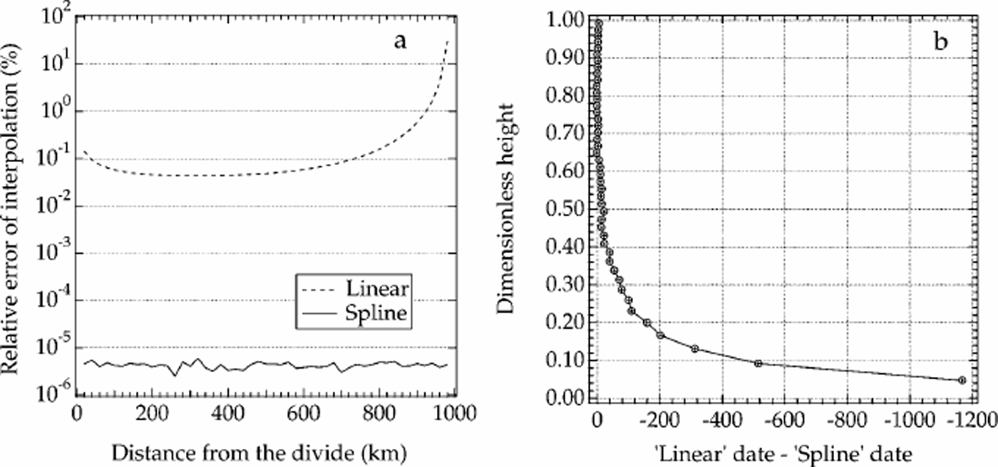
(a) Relative error of interpolation (%) of the linear and the cubic-spline methods for the horizontal velocity in the experiment. (b) Cumulative error on date of deposition using linear interpolation in the Lagrangian scheme at a position from the divide.

3.5. Problems of interpolation in the Lagrangian approach

The problem of applying the Lagrangian approach and comparing it with the Eulerian method is fundamentally a problem of interpolation. Since the velocity field is prescribed on a regular grid, and a particle’s position needs to be obtained in any point during a model run, one has to interpolate the velocity field between gridpoints to obtain spatial increments of a particle’s position. Further, since the position of a particle is computed step by step, these errors are cumulative. The second problem arises from the comparison itself and is due to uneven spatial coverage of tracers. The only solution to the latter problem is a higher abundance of initial tracers. A preliminary analysis of the flow is therefore necessary to decide at which location, and at which frequency in time-dependent applications, additional tracers need to be launched.

Concerning the first problem, it is clear that bi-cubicspline interpolation is better than piecewise bilinear interpolation. This is demonstrated in Figure 4. In Figure 4a we compute the modulus of the relative error of both methods of interpolation for the horizontal velocity with respect to the analytical result as given by Equation (8), and average the result over the vertical coordinate. That provides a good measure of interpolation errors. It can be seen that spline interpolation of the horizontal velocity is three to as much as seven orders of magnitude more accurate than linear interpolation. In our schematic set-up, the interpolation error on velocity almost exclusively originates from the horizontal velocity component because the vertical velocity is linear, and therefore both interpolation methods give similar results for the vertical to within computer accuracy. Based on the results shown in Figure 4a, we can safely consider the spline interpolation results as the reference state to assess the accuracy of the linear interpolation method.

We find that linear interpolation generally leads to underestimation of the velocity and therefore to smaller displacements and a calculated date of deposition that is earlier as compared to the spline method. This fact is illustrated in Figure 4b, where the cumulative error on date is shown for the transect at the margin at x = 980 km. Still, the absolute value of accumulated error on date of deposition of approximately 1200 years in the lower layers corresponds to a relative error of 51.5%. Similar results were obtained at other locations closer to the divide, giving a typical relative error on date by linear interpolation of about 1% at 90% depth.

The difference between the two methods of date estimation is therefore small, and linear interpolation can be expected to yield acceptable results. This is the more so in view of the large central processing unit (CPU) time required for spline interpolation whose magnitude makes it hardly applicable in a three-dimensional ice-sheet model. The main reason is that spline interpolation is not a local interpolation technique but requires calculation of two partial derivatives at the tracer’s position at every time-step (Reference Press, Teukolsky, Vetterling and FlanneryPress and others, 1992). In three-dimensional applications, the additional CPU cost is at least two orders of magnitude larger than for linear interpolation.

4.1. Experimental set-up

To assess the applicability of the two dating methods under real conditions, we implemented the age-calculation routines in a three-dimensional thermomechanical model of the Antarctic ice sheet (Reference HuybrechtsHuybrechts and de Wolde, 1999; Reference Huybrechts and de WoldeHuybrechts, 2002). This model is time-dependent, calculates the coupled velocity and temperature fields, and has components describing basal sliding, basal melting, the surface climate, isostatic adjustment, and the flow in a coupled ice shelf. The horizontal resolution is 20 km and there are 31 layers in the vertical, gradually decreasing in thickness towards the base. The model employs a dimensionless vertical coordinate scaled to ice thickness with grid spacings of 5% of ice thickness at the surface and 1% at the base.

The model was run for stationary present-day climatic conditions. The only constraint compared to recent applications of the model is that the grounding line was fixed to its current position. Ice thickness is, however, still a free variable allowed to establish an equilibrium with the climate forcing and the flow law. Consequently, the vertical velocity is obtained from the continuity equation and retains full consistency with the horizontal velocity components and the surface mass balance, which is positive over the entire model domain. Basal melting and basal sliding occur in the model whenever basal temperature reaches the pressure-melting point. The Antarctic experiment therefore combines all of the features discussed in the schematic experiments above, with the notable exception that vertical velocity is no longer linear.

For the Eulerian ice-date computations, the same second-order upwinding scheme was used as in the schematic experiments, and, for the Lagrangian method, piecewise linear interpolation was applied for tracking tracer position in between gridpoints. The calculations took place directly within the transformed coordinate system, ensuring that vertical movement is always directed downwards over the entire model domain, thus avoiding basal boundary-condition problems in the upwinding advection scheme. For the Lagrangian computations, tracers were launched only once at the surface at the initial time for every grounded gridpoint. The total number of tracers therefore equalled approximately 30500 out of a total number of 281×281=78961 horizontal gridpoints. The total integration time was 500 kyr for both methods, with a time-step of 5 years. This is a long enough period to ensure that a stationary solution is established for the advection equation and that all tracers that have remained within the grounded ice sheet are well below 90% depth. For the Eulerian calculations, the initial condition on date of deposition consisted of the analytical result given by Equation (11). To facilitate the experiment, the Lagrangian run was actually run in offline mode with the velocity output from the Antarctic model for the present time.

4.2. Results

Figure 5 shows an example of the resulting distributions of the date of deposition at an intermediate depth of 60%. These results should not be confused with the“real”date distribution in the Antarctic ice sheet since ice thickness and accumulation rate have not been allowed to vary over the full length of the integration period in response to climatic changes (though the accumulation rate has changed in accordance with surface elevation changes relative to the observations). Nevertheless, the pattern is expected to be qualitatively similar to reality, with old ice concentrated in the interior of East Antarctica roughly inversely proportional to the surface accumulation rate, together with much younger ice at comparable relative depth in West Antarctica and at the margin. Also clear are the effects of flow divergence/convergence and of the flow chanelling into the outlet glaciers that drain most of the ice sheet at the margin. In general, the two methods give very similar results, with absolute date differences of maximally ±10 kyr, but well below ±2 kyr over most of the area, with the Lagrangian method giving some what older ice at the margin and somewhat younger ice in the interior (Fig. 5).

Fig. 5.

Date of deposition computed in the Antarctic ice sheet for present-day stationary climatic conditions by both methods, as well as their absolute difference. This example is for the layer at 60% depth.

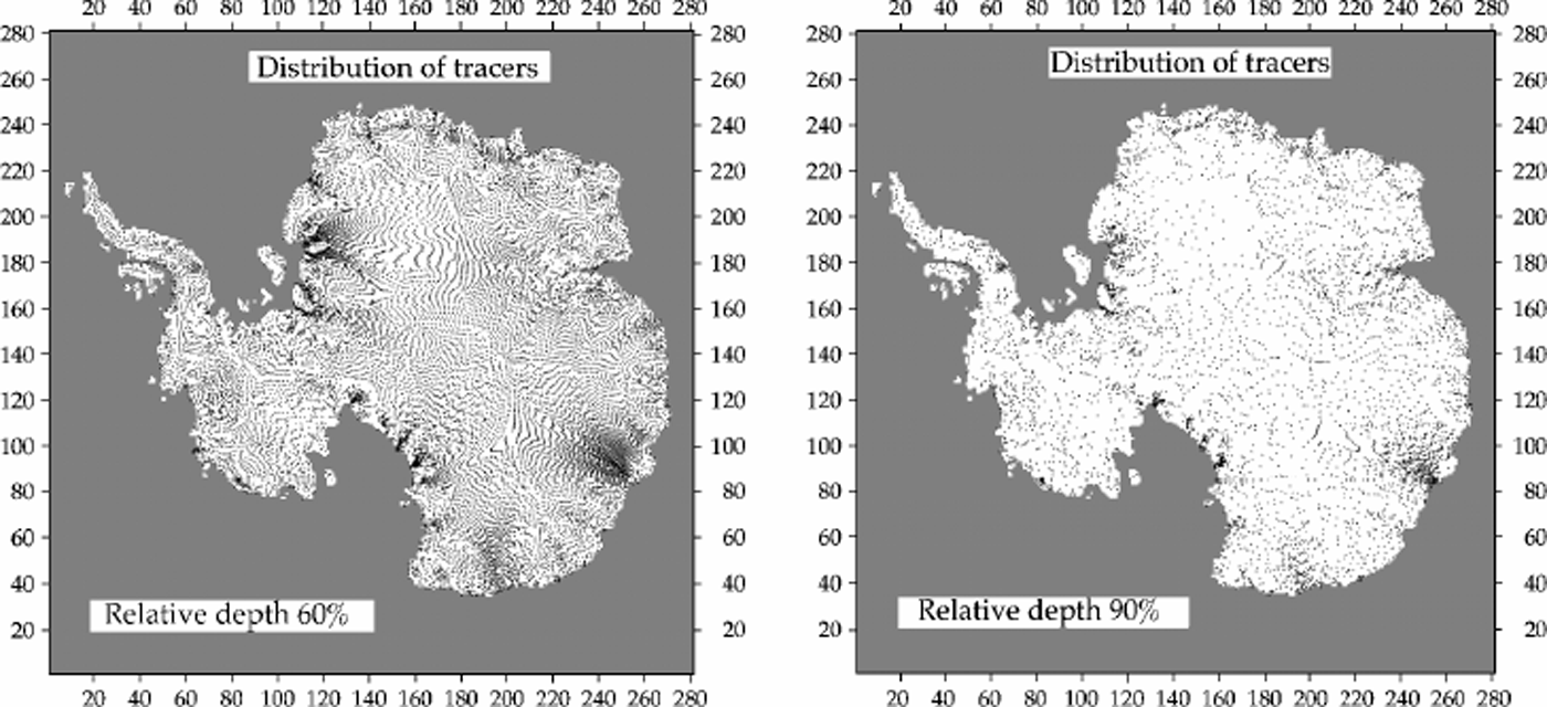
However, the largest differences occur in zones of large gradients and can therefore be explained by diffusive effects in the Eulerian scheme and, probably more importantly, the irregular distribution of tracers that results for deeper layers in the Lagrangian method. This is demonstrated in more detail in Figure 6, marking the positions where tracers have crossed a given depth layer during the course of the integration. At a relative depth of 60%, only half of the original tracers remain in the ice sheet, and the other half have migrated into the surrounding ice shelves or have been washed out in the ocean. At 90% depth, less than a quarter of the tracers remain, and they are distributed unevenly in space. It should, however, be noted that this problem will be less severe when tracers are launched at regular time intervals in time-depend-ent applications with changing climatic input and ice-sheet geometry.

Fig. 6.

Distribution of tracer crossings through the 60% and 90% depth layers in the Antarctic experiment, showing how tracers are gradually concentrated and washed out towards the margin in deeper layers. In this experiment, tracers were launched only once for every ice-sheet gridpoint on the 2816281 numerical mesh.

The inverse problem, in which the tracers are used to compute the relative depth of an isochrone surface, does not depend on the rhythm by which tracers are launched at the surface. Figure 7 shows the distribution of the final positions of tracers 100 kyr after they were launched at the surface. In our steady-state experiment, these are the points one would have to use to reconstruct the depth of the 100 kyr isochrone surface. Almost all of the remaining tracers concentrate within interior East Antarctica, with a very sparse distribution at the margin and in West Antarctica, and virtually none in the Antarctic Peninsula area. In this case, the isochrone surface of 100 kyr is marked by only 310 9 tracers out of the 30548 initially inserted at the surface.

Fig. 7.

Distribution of tracers at the depth of the isochrone surface of 100 kyr in the Antarctic model, demonstrating the problem of tracer density for interpolating age horizons on a regular numerical grid.